On the Simultaneous Solution of Structural Membranes on all Level Sets within a Bulk Domain

Abstract

A mechanical model and numerical method for structural membranes implied by all isosurfaces of a level-set function in a three-dimensional bulk domain are proposed. The mechanical model covers large displacements in the context of the finite strain theory and is formulated based on the tangential differential calculus. Alongside curved two-dimensional membranes embedded in three dimensions, also the simpler case of curved ropes (cables) in two-dimensional bulk domains is covered. The implicit geometries (shapes) are implied by the level sets and the boundaries of the structures are given by the intersection of the level sets with the boundary of the bulk domain. For the numerical analysis, the bulk domain is discretized using a background mesh composed by (higher-order) elements with the dimensionality of the embedding space. The elements are by no means aligned to the level sets, i.e., the geometries of the structures, which resembles a fictitious domain method, most importantly the Trace FEM. The proposed numerical method is a hybrid of the classical FEM and fictitious domain methods which may be labeled as “Bulk Trace FEM”. Numerical studies confirm higher-order convergence rates and the potential for new material models with continuously embedded sub-structures in bulk domains.

Keywords: finite strain theory, ropes, membranes, Trace FEM, fictitious domain method, embedded domain method, PDEs on manifolds, implicit geometry, level-set method

1 Introduction

One may classify models in structural mechanics based on their dimensionality which is mostly related to their geometric properties. For example, thin structures with one prominent direction subjected to bending may often be modeled as one-dimensional beams, and flat structures with small thickness as plates. For straight beams and plates, one may thereby reduce the dimensionality of the naturally three-dimensional structure to 1 or 2, respectively, often resulting in largely simplified boundary value problems (BVPs) compared to the original, three-dimensional case. However, for curved structures such as curved beams, membranes and shells [5, 15, 20, 17, 45], the situation is often more complex as they are embedded in some exterior space with higher dimensionality. As the deformation takes place in this background space, the complexity is still related to the dimensionality of the background space. Furthermore, due to the curvature of the lower-dimensional structures, differential geometry becomes an inherent part of the mechanical models, i.e., the resulting BVPs. In this work, the focus is on structural membranes being curved two-dimensional structures in three dimensions undergoing large displacements; the simpler reduction of this scenario are curved one-dimensional ropes (cables) in two dimensions.

Curved lower-dimensional manifolds such as curved lines in 2D and curved surfaces in 3D may be defined explicitly through parametrizations [25, 63, 24, 30] or implicitly through the level-set method [54, 53, 62]. In the latter case, often the zero-level set of some scalar function implies the domain of interest (e.g., the geometry of one membrane). However, it is important to note that a level-set function, in fact, implies infinitely many level sets featuring different constant values each. One may then ask for a successive analysis of different curved structures implied by (some) selected level sets. It turns out that the displacement fields in the vicinity of a selected level set (typically) vary smoothly, suggesting that it is possible to formulate a mechanical model for the displacement field of all structures implied by all level sets within some bulk domain at once; such a model and the related numerical analysis are in the focus of this work. Innovative applications of the proposed mechanical model may be found in new material models where some (elastic) bulk material is equipped with embedded sub-structures (i.e., continuously distributed fibres and membranes), introducing a new concept of anisotropy. The simultaneous analysis of structures also features advantages in design and optimization as minimal and maximal values of displacements or stress quantities are immediately obtained for a whole family of geometries (i.e., all level sets).

The basic idea is outlined as follows: Let there be some undeformed bulk domain with the dimensionality of the embedding space and a level-set function. The level sets inside the bulk domain imply infinitely many bounded, curved manifolds of codimension 1, which herein represent a set of curved, undeformed membranes in 3D or ropes in 2D, respectively. We now seek a mechanical model which determines the displacement field of the bulk domain, such that the level sets interpreted in this deformed bulk domain are the deformed structures (membranes). Therefore, a finite strain theory is formulated in the frame of the tangential differential calculus (TDC). With TDC, we only refer to the modern differential geometric point of view of formulating BVPs on curved manifolds based on surface differential operators rather than on local curvilinear coordinate systems and Christoffel symbols. The advantages of the TDC-framework have already been demonstrated by the authors in [36], with focus on generalizing the geometrical, mechanical and numerical description and treatment of single membranes, see also [59, 58] for shells. The potential for simultaneous multi-membrane studies on all level sets was not foreseen at that point, yet it may now be seen as another important advantage of proposing mechanical models for curved structures in the frame of the TDC.

For the numerical analysis, the (undeformed) bulk domain is discretized using higher-order elements of the same dimensionality as the embedding space. The elements conform to the boundary of the bulk domain, however, they are by no means aligned to the level sets which imply the actual shape of the structures. This may be interpreted as a hybrid between the classical FEM and fictitious or embedding domain methods. Here, classical FEM refers to a single-membrane study employing a surface mesh which conforms to the shape and boundary of the membrane; this may also be called the Surface FEM. A fictitious domain approach for a single-membrane study would be to use, e.g., the Cut FEM or Trace FEM as presented in [36] where a background mesh is employed that neither conforms to the shape nor the boundary of the membrane of interest, see also [8, 9, 10] for general references on the Cut FEM and [50, 55, 38] for the Trace FEM. Just as most fictitious domain methods, the Trace FEM comes at the price of dealing with cut elements in terms of integration and stabilization and increased efforts in considering boundary conditions. The method presented here does also use a background mesh in the bulk domain, however, without any need for cut elements and boundary conditions are prescribed as usual in the classical FEM. In this sense, it resembles most features of the classical FEM, yet it is emphasized that $d$-dimensional background elements are used to simultaneously analyze a set of curved, $\left(d-1\right)$-dimensional structures.

It seems natural to label the resulting approach, which herein is applied in the context of structural membranes and ropes (in large displacement theory), the “Bulk Trace FEM”. The most important fact that the domains of interest are imposed by level sets justifies the use of the term “Trace FEM” and the addition of “bulk” refers to the fact that rather than solving a BVP on one level set, it is solved simultaneously on all level sets in some bulk domain.

To the best of the author’s knowledge, we are not aware of similar approaches for the simultaneous modeling and analysis of curved, lower-dimensional structures, even less so in the context of large displacements. However, for flow and transport problems, models for the simultaneous solution on all level sets are found, e.g., in [2, 27, 26] and for some elliptic partial differential equations in [6]. Often, low-order meshes are employed in the bulk domains and the transport takes place on closed level sets so that boundary conditions play a minor role. Then, the emphasis is often on transient problems and possibly moving bulk domains [2, 26]. For an overview of finite element methods for PDEs on surfaces in general and an introduction on the simultaneous analysis on all level sets within a bulk domain for some elliptic and parabolic PDEs, see [29]. Minimizing the bulk domain to a narrow band around some selected level set of interest leads to the narrow-band method proposed in [21, 22]. Narrow-band methods based on finite differences on a standard Cartesian grid for transport problems are presented in [4, 40, 41]. As mentioned before, when the solution on a single level set is sought, fictitious domain methods such as the Trace FEM and Cut FEM may be used as presented, e.g., in [52, 50, 19, 39, 11, 13, 14]. In structural mechanics, Cut and Trace FEM approaches are published in [16] for linear membranes, [61] for Reissner-Mindlin shells, [37] for Kirchhoff-Love shells and in [36] for non-linear ropes and membranes in large displacement theory.

The paper is organized as follows: The general concept of using level sets over bulk domains for the implicit and simultaneous geometry definition of curved structures is outlined in Section 2, including the definition of tangential differential operators on the level sets. The mechanical setup in the context of large displacement theory is outlined in Section 3, where reference and spatial configurations are distinguished and equilibrium is enforced in the latter. The complete BVP for the simultaneous mechanical modeling on all level sets in the bulk domain is given, including boundary conditions. When the bulk domain is optionally equipped with mechanical properties (e.g., an elastic bulk material), the concept of continuously embedded sub-structure models is outlined in Section 3.7. The Bulk Trace FEM for the numerical approximation of the BVP is defined in Section 4. Numerical results are presented in Section 5 in two- and three-dimensional bulk domains and demonstrate higher-order convergence rates provided that the solutions of the BVP are sufficiently smooth. The paper ends in Section 6 with a summary and conclusions.

2 Level sets in bulk domains: Geometric setup and differential operators

Before dealing with the mechanical setup in terms of deformed and undeformed configurations in finite strain theory, the situation is first outlined generically with focus on geometric quantities as implied by the level sets within some bulk domain and resulting differential operators.

2.1 Bulk domains and level-set functions

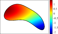
(a) $\Omega$ and $\phi$

(b) $\Omega$ and level sets of $\phi$

(c) $\Omega$ and level sets $\Gamma^{c}$

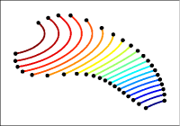
(d) level sets $\Gamma^{c}$

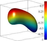
(e) $\Omega$ and $\phi$

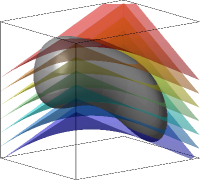
(f) $\Omega$ and level sets of $\phi$

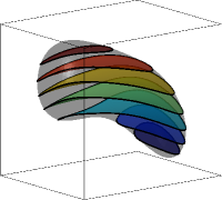
(g) $\Omega$ and level sets $\Gamma^{c}$

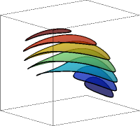
(h) level sets $\Gamma^{c}$

Figure 1: Some bulk domain $\Omega$ and level-set function $\phi\left(\mathchoice{\displaystyle\boldsymbol{x}}{\textstyle\boldsymbol{x}}{\scriptstyle\boldsymbol{x}}{\scriptscriptstyle\boldsymbol{x}}\right)$ in two and three dimensions and the implied level sets $\Gamma^{c}$.

Let there be a $d$-dimensional bulk domain $\Omega\subset\mathbb{R}^{d}$ and a level-set function $\phi\left(\mathchoice{\displaystyle\boldsymbol{x}}{\textstyle\boldsymbol{x}}{\scriptstyle\boldsymbol{x}}{\scriptscriptstyle\boldsymbol{x}}\right):\Omega\rightarrow\mathbb{R}$. We call the smallest and largest value of $\phi$ in the bulk domain $\phi^{\min}=\inf\phi\left(\mathchoice{\displaystyle\boldsymbol{x}}{\textstyle\boldsymbol{x}}{\scriptstyle\boldsymbol{x}}{\scriptscriptstyle\boldsymbol{x}}\right)$ and $\phi^{\max}=\sup\phi\left(\mathchoice{\displaystyle\boldsymbol{x}}{\textstyle\boldsymbol{x}}{\scriptstyle\boldsymbol{x}}{\scriptscriptstyle\boldsymbol{x}}\right)$. Then, the individual level sets $\Gamma^{c}$ related to constant level-set values $c\in\mathbb{R}$,

$$\Gamma^{c}=\left\{\mathchoice{\displaystyle\boldsymbol{x}}{\textstyle\boldsymbol{x}}{\scriptstyle\boldsymbol{x}}{\scriptscriptstyle\boldsymbol{x}}\in\Omega:\,\phi(\mathchoice{\displaystyle\boldsymbol{x}}{\textstyle\boldsymbol{x}}{\scriptstyle\boldsymbol{x}}{\scriptscriptstyle\boldsymbol{x}})=c\in\mathbb{R}\right\},\,\phi^{\min}<c<\phi^{\max},$$ (2.1)

are bounded, typically curved, $(d-1)$-dimensional manifolds (i.e., they have codimension $1$), see Fig. 1. Consequently, the set of all bounded level sets $\Gamma^{c}$ coincides with $\Omega$. The boundary of the bulk domain $\Omega$ is called $\partial\Omega$. The boundary of some level set $\Gamma^{c}$ is labeled $\partial\Gamma^{c}$ and is the intersection point or line of the level set with constant value $c$ and the boundary of the background domain $\partial\Omega$, see again Fig. 1. As such, the set of all $\partial\Gamma^{c}$ coincides with $\partial\Omega$.

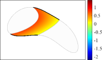
(a) $\Omega$ and $\phi$

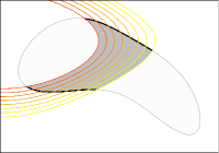
(b) $\Omega$ and level sets of $\phi$

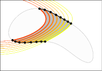
(c) $\Omega$ and level sets $\Gamma^{c}$

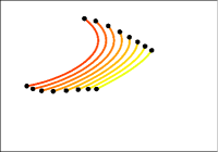
(d) level sets $\Gamma^{c}$

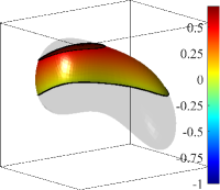
(e) $\Omega$ and $\phi$

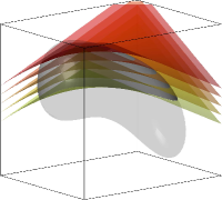
(f) $\Omega$ and level sets of $\phi$

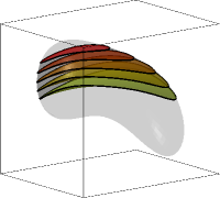
(g) $\Omega$ and level sets $\Gamma^{c}$

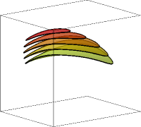
(h) level sets $\Gamma^{c}$

Figure 2: The bulk domains $\Omega$ resulting from some larger $\Omega^{\text{sup}}$ in two and three dimensions and a prescribed level-set interval $\left[\phi^{\min},\phi^{\max}\right]$. Some selected level sets $\Gamma^{c}$ in this interval are also shown.

Instead of defining the bulk domain of interest $\Omega$ directly with resulting $\phi^{\min}$ and $\phi^{\max}$, one may also prescribe $\Omega$ indirectly by first defining a superset of the bulk domain, say $\Omega^{\sup}\subset\mathbb{R}^{d}$, and then limit the bulk domain of interest $\Omega$ using specified values for $\phi^{\min}$ and $\phi^{\max}$,

$$\Omega=\left\{\mathchoice{\displaystyle\boldsymbol{x}}{\textstyle\boldsymbol{x}}{\scriptstyle\boldsymbol{x}}{\scriptscriptstyle\boldsymbol{x}}\in\Omega^{\sup}:\phi^{\min}\leq\phi(\mathchoice{\displaystyle\boldsymbol{x}}{\textstyle\boldsymbol{x}}{\scriptstyle\boldsymbol{x}}{\scriptscriptstyle\boldsymbol{x}})\leq\phi^{\max}\right\},$$ (2.2)

see Fig. 2. In this case, the level sets $\Gamma^{c}$ and their boundaries $\partial\Gamma^{c}$ are defined as before, however, we shall restrict the boundary of the bulk domain $\partial\Omega$ to those parts of the boundary where $\phi\left(\mathchoice{\displaystyle\boldsymbol{x}}{\textstyle\boldsymbol{x}}{\scriptstyle\boldsymbol{x}}{\scriptscriptstyle\boldsymbol{x}}\right)\neq\phi^{\min}$ and $\phi\left(\mathchoice{\displaystyle\boldsymbol{x}}{\textstyle\boldsymbol{x}}{\scriptstyle\boldsymbol{x}}{\scriptscriptstyle\boldsymbol{x}}\right)\neq\phi^{\max}$.

2.2 Normal and conormal vectors

The boundary of the bulk domain $\partial\Omega$ features a unit normal vector (field) $\mathchoice{\displaystyle\boldsymbol{m}}{\textstyle\boldsymbol{m}}{\scriptstyle\boldsymbol{m}}{\scriptscriptstyle\boldsymbol{m}}\left(\mathchoice{\displaystyle\boldsymbol{x}}{\textstyle\boldsymbol{x}}{\scriptstyle\boldsymbol{x}}{\scriptscriptstyle\boldsymbol{x}}\right)$, $\mathchoice{\displaystyle\boldsymbol{x}}{\textstyle\boldsymbol{x}}{\scriptstyle\boldsymbol{x}}{\scriptscriptstyle\boldsymbol{x}}\in\partial\Omega$. Depending on whether the bulk domain is defined through a parametrization or implicitly, these normal vectors may be obtained through different definitions. However, because the bulk domain is later discretized by higher-order elements for the numerical analysis, see Section 5, the generation of $\mathchoice{\displaystyle\boldsymbol{m}}{\textstyle\boldsymbol{m}}{\scriptstyle\boldsymbol{m}}{\scriptscriptstyle\boldsymbol{m}}$ on element boundaries is a standard task in the FEM and not further outlined here.

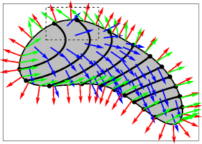
(a) vectors $\mathchoice{\displaystyle\boldsymbol{n}}{\textstyle\boldsymbol{n}}{\scriptstyle\boldsymbol{n}}{\scriptscriptstyle\boldsymbol{n}}$, $\mathchoice{\displaystyle\boldsymbol{m}}{\textstyle\boldsymbol{m}}{\scriptstyle\boldsymbol{m}}{\scriptscriptstyle\boldsymbol{m}}$, $\mathchoice{\displaystyle\boldsymbol{q}}{\textstyle\boldsymbol{q}}{\scriptstyle\boldsymbol{q}}{\scriptscriptstyle\boldsymbol{q}}$

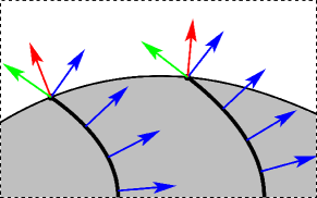
(b) zoom

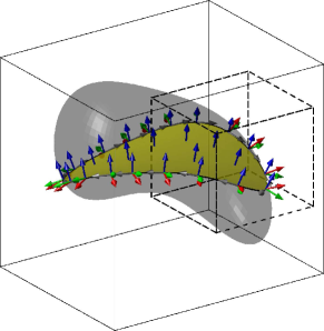
(c) vectors $\mathchoice{\displaystyle\boldsymbol{n}}{\textstyle\boldsymbol{n}}{\scriptstyle\boldsymbol{n}}{\scriptscriptstyle\boldsymbol{n}}$, $\mathchoice{\displaystyle\boldsymbol{m}}{\textstyle\boldsymbol{m}}{\scriptstyle\boldsymbol{m}}{\scriptscriptstyle\boldsymbol{m}}$, $\mathchoice{\displaystyle\boldsymbol{t}}{\textstyle\boldsymbol{t}}{\scriptstyle\boldsymbol{t}}{\scriptscriptstyle\boldsymbol{t}}$, $\mathchoice{\displaystyle\boldsymbol{q}}{\textstyle\boldsymbol{q}}{\scriptstyle\boldsymbol{q}}{\scriptscriptstyle\boldsymbol{q}}$

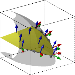
(d) zoom

Figure 3: Vector fields in the domain $\Omega$ and on the boundary $\partial\Omega$ in two and three dimensions, the right figures show zooms of the left ones. Normal vectors $\mathchoice{\displaystyle\boldsymbol{n}}{\textstyle\boldsymbol{n}}{\scriptstyle\boldsymbol{n}}{\scriptscriptstyle\boldsymbol{n}}$ with respect to the level sets $\Gamma^{c}$ in $\Omega$ are shown in blue. Normal vectors $\mathchoice{\displaystyle\boldsymbol{m}}{\textstyle\boldsymbol{m}}{\scriptstyle\boldsymbol{m}}{\scriptscriptstyle\boldsymbol{m}}$ with respect to $\partial\Omega$ are red, tangential vectors $\mathchoice{\displaystyle\boldsymbol{t}}{\textstyle\boldsymbol{t}}{\scriptstyle\boldsymbol{t}}{\scriptscriptstyle\boldsymbol{t}}$ are gray and conormal vectors $\mathchoice{\displaystyle\boldsymbol{q}}{\textstyle\boldsymbol{q}}{\scriptstyle\boldsymbol{q}}{\scriptscriptstyle\boldsymbol{q}}$ are green.

The unit normal vector (field) $\mathchoice{\displaystyle\boldsymbol{n}}{\textstyle\boldsymbol{n}}{\scriptstyle\boldsymbol{n}}{\scriptscriptstyle\boldsymbol{n}}\left(\mathchoice{\displaystyle\boldsymbol{x}}{\textstyle\boldsymbol{x}}{\scriptstyle\boldsymbol{x}}{\scriptscriptstyle\boldsymbol{x}}\right)$ on the level sets $\Gamma^{c}$ in the whole bulk domain $\Omega$ is obtained by the gradient of the level-set function,

$$\mathchoice{\displaystyle\boldsymbol{n}}{\textstyle\boldsymbol{n}}{\scriptstyle\boldsymbol{n}}{\scriptscriptstyle\boldsymbol{n}}\left(\mathchoice{\displaystyle\boldsymbol{x}}{\textstyle\boldsymbol{x}}{\scriptstyle\boldsymbol{x}}{\scriptscriptstyle\boldsymbol{x}}\right)=\frac{\mathchoice{\displaystyle\boldsymbol{n}}{\textstyle\boldsymbol{n}}{\scriptstyle\boldsymbol{n}}{\scriptscriptstyle\boldsymbol{n}}^{\star}}{\left\|\mathchoice{\displaystyle\boldsymbol{n}}{\textstyle\boldsymbol{n}}{\scriptstyle\boldsymbol{n}}{\scriptscriptstyle\boldsymbol{n}}^{\star}\right\|}\quad\textrm{with}\quad\mathchoice{\displaystyle\boldsymbol{n}}{\textstyle\boldsymbol{n}}{\scriptstyle\boldsymbol{n}}{\scriptscriptstyle\boldsymbol{n}}^{\star}=\nabla\phi\left(\mathchoice{\displaystyle\boldsymbol{x}}{\textstyle\boldsymbol{x}}{\scriptstyle\boldsymbol{x}}{\scriptscriptstyle\boldsymbol{x}}\right),\;\mathchoice{\displaystyle\boldsymbol{x}}{\textstyle\boldsymbol{x}}{\scriptstyle\boldsymbol{x}}{\scriptscriptstyle\boldsymbol{x}}\in\Omega.$$ (2.3)

One may then also construct the projector field $\mathchoice{\displaystyle\mathbf{p}}{\textstyle\mathbf{p}}{\scriptstyle\mathbf{p}}{\scriptscriptstyle\mathbf{p}}\left(\mathchoice{\displaystyle\boldsymbol{x}}{\textstyle\boldsymbol{x}}{\scriptstyle\boldsymbol{x}}{\scriptscriptstyle\boldsymbol{x}}\right)\in\mathbb{R}^{d\times d}$, $\mathchoice{\displaystyle\boldsymbol{x}}{\textstyle\boldsymbol{x}}{\scriptstyle\boldsymbol{x}}{\scriptscriptstyle\boldsymbol{x}}\in\Omega$,

$$\mathchoice{\displaystyle\mathbf{p}}{\textstyle\mathbf{p}}{\scriptstyle\mathbf{p}}{\scriptscriptstyle\mathbf{p}}\left(\mathchoice{\displaystyle\boldsymbol{x}}{\textstyle\boldsymbol{x}}{\scriptstyle\boldsymbol{x}}{\scriptscriptstyle\boldsymbol{x}}\right)=\mathchoice{\displaystyle\mathbf{I}}{\textstyle\mathbf{I}}{\scriptstyle\mathbf{I}}{\scriptscriptstyle\mathbf{I}}-\mathchoice{\displaystyle\boldsymbol{n}}{\textstyle\boldsymbol{n}}{\scriptstyle\boldsymbol{n}}{\scriptscriptstyle\boldsymbol{n}}\otimes\mathchoice{\displaystyle\boldsymbol{n}}{\textstyle\boldsymbol{n}}{\scriptstyle\boldsymbol{n}}{\scriptscriptstyle\boldsymbol{n}}.$$ (2.4)

The unit conormal vectors $\mathchoice{\displaystyle\boldsymbol{q}}{\textstyle\boldsymbol{q}}{\scriptstyle\boldsymbol{q}}{\scriptscriptstyle\boldsymbol{q}}\left(\mathchoice{\displaystyle\boldsymbol{x}}{\textstyle\boldsymbol{x}}{\scriptstyle\boldsymbol{x}}{\scriptscriptstyle\boldsymbol{x}}\right)$ on $\partial\Omega$ are in the tangent plane of the corresponding level sets at $\partial\Gamma^{c}$ and yet normal to $\mathchoice{\displaystyle\boldsymbol{n}}{\textstyle\boldsymbol{n}}{\scriptstyle\boldsymbol{n}}{\scriptscriptstyle\boldsymbol{n}}\left(\mathchoice{\displaystyle\boldsymbol{x}}{\textstyle\boldsymbol{x}}{\scriptstyle\boldsymbol{x}}{\scriptscriptstyle\boldsymbol{x}}\right)$ from above. In case of two-dimensional bulk domains, $d=2$, see Figs. 3(a) and (b), these vectors are defined without the normal vectors of the bulk domains $\mathchoice{\displaystyle\boldsymbol{m}}{\textstyle\boldsymbol{m}}{\scriptstyle\boldsymbol{m}}{\scriptscriptstyle\boldsymbol{m}}$ and are simply obtained from $\mathchoice{\displaystyle\boldsymbol{n}}{\textstyle\boldsymbol{n}}{\scriptstyle\boldsymbol{n}}{\scriptscriptstyle\boldsymbol{n}}=[n_{x},\;n_{y}]^{\mathrm{T}}$ as

$$\mathchoice{\displaystyle\boldsymbol{q}}{\textstyle\boldsymbol{q}}{\scriptstyle\boldsymbol{q}}{\scriptscriptstyle\boldsymbol{q}}\left(\mathchoice{\displaystyle\boldsymbol{x}}{\textstyle\boldsymbol{x}}{\scriptstyle\boldsymbol{x}}{\scriptscriptstyle\boldsymbol{x}}\right)=\left[\begin{array}[]{c}q_{x}\\ q_{y}\end{array}\right]=\left[\begin{array}[]{c}-n_{y}\\ n_{x}\end{array}\right].$$

For three-dimensional bulk domains, $d=3$, see Figs. 3(c) and (d), one needs to first generate tangent vector fields $\mathchoice{\displaystyle\boldsymbol{t}}{\textstyle\boldsymbol{t}}{\scriptstyle\boldsymbol{t}}{\scriptscriptstyle\boldsymbol{t}}\left(\mathchoice{\displaystyle\boldsymbol{x}}{\textstyle\boldsymbol{x}}{\scriptstyle\boldsymbol{x}}{\scriptscriptstyle\boldsymbol{x}}\right)$ on $\partial\Omega$ using cross products of the normal vector fields from above, $\mathchoice{\displaystyle\boldsymbol{t}}{\textstyle\boldsymbol{t}}{\scriptstyle\boldsymbol{t}}{\scriptscriptstyle\boldsymbol{t}}=\mathchoice{\displaystyle\boldsymbol{m}}{\textstyle\boldsymbol{m}}{\scriptstyle\boldsymbol{m}}{\scriptscriptstyle\boldsymbol{m}}\times\mathchoice{\displaystyle\boldsymbol{n}}{\textstyle\boldsymbol{n}}{\scriptstyle\boldsymbol{n}}{\scriptscriptstyle\boldsymbol{n}}$, and then

$$\mathchoice{\displaystyle\boldsymbol{q}}{\textstyle\boldsymbol{q}}{\scriptstyle\boldsymbol{q}}{\scriptscriptstyle\boldsymbol{q}}=\frac{\mathchoice{\displaystyle\boldsymbol{q}}{\textstyle\boldsymbol{q}}{\scriptstyle\boldsymbol{q}}{\scriptscriptstyle\boldsymbol{q}}^{\star}}{\left\|\mathchoice{\displaystyle\boldsymbol{q}}{\textstyle\boldsymbol{q}}{\scriptstyle\boldsymbol{q}}{\scriptscriptstyle\boldsymbol{q}}^{\star}\right\|}\,\,\textrm{with}\,\,\mathchoice{\displaystyle\boldsymbol{q}}{\textstyle\boldsymbol{q}}{\scriptstyle\boldsymbol{q}}{\scriptscriptstyle\boldsymbol{q}}^{\star}=\mathchoice{\displaystyle\boldsymbol{n}}{\textstyle\boldsymbol{n}}{\scriptstyle\boldsymbol{n}}{\scriptscriptstyle\boldsymbol{n}}\times\mathchoice{\displaystyle\boldsymbol{t}}{\textstyle\boldsymbol{t}}{\scriptstyle\boldsymbol{t}}{\scriptscriptstyle\boldsymbol{t}}.$$

These conormal vector fields will later play an important role in the weak formulation of the boundary value problem and the definition of boundary conditions. It is noted that for the indirect definition of the bulk domain $\Omega$ according to Eq. (2.2), conormal vectors may only be defined on those parts of the whole boundary of $\Omega$ which do not coincide with level sets, because there $\mathchoice{\displaystyle\boldsymbol{m}}{\textstyle\boldsymbol{m}}{\scriptstyle\boldsymbol{m}}{\scriptscriptstyle\boldsymbol{m}}=\mathchoice{\displaystyle\boldsymbol{n}}{\textstyle\boldsymbol{n}}{\scriptstyle\boldsymbol{n}}{\scriptscriptstyle\boldsymbol{n}}$ and tangential vectors $\mathchoice{\displaystyle\boldsymbol{t}}{\textstyle\boldsymbol{t}}{\scriptstyle\boldsymbol{t}}{\scriptscriptstyle\boldsymbol{t}}$ may not be computed through cross products. This is why in Section 2.1, those parts of the boundary of the bulk domain were excluded from $\partial\Omega$. In other words, $\partial\Omega$ is the boundary of the bulk domain $\Omega$ where $\mathchoice{\displaystyle\boldsymbol{m}}{\textstyle\boldsymbol{m}}{\scriptstyle\boldsymbol{m}}{\scriptscriptstyle\boldsymbol{m}}\neq\mathchoice{\displaystyle\boldsymbol{n}}{\textstyle\boldsymbol{n}}{\scriptstyle\boldsymbol{n}}{\scriptscriptstyle\boldsymbol{n}}$ and, hence, conormal vectors $\mathchoice{\displaystyle\boldsymbol{q}}{\textstyle\boldsymbol{q}}{\scriptstyle\boldsymbol{q}}{\scriptscriptstyle\boldsymbol{q}}$ exist, see, e.g., the black line in Fig. 2(c).

2.3 Differential operators with respect to level sets

For the definition of BVPs on the level sets, it is important to distinguish (classical) differential operators acting in the bulk space (such as the gradient $\nabla$ in Eq. (2.3)) from differential operators acting on the level sets which may be called tangential or surface operators (although, for two-dimensional bulk domains, the level sets are rather curved lines). The surface gradient of a scalar function $f\!\left(\mathchoice{\displaystyle\boldsymbol{x}}{\textstyle\boldsymbol{x}}{\scriptstyle\boldsymbol{x}}{\scriptscriptstyle\boldsymbol{x}}\right):\Omega\to\mathbb{R}$ results as [24, 28, 46, 60]

$$\nabla^{\Gamma}f=\mathchoice{\displaystyle\mathbf{p}}{\textstyle\mathbf{p}}{\scriptstyle\mathbf{p}}{\scriptscriptstyle\mathbf{p}}\cdot\nabla f,$$ (2.5)

where $\nabla f$ is the classical gradient in the $d$-dimensional space. It is noted that $\nabla^{\Gamma}\phi=\mathchoice{\displaystyle\boldsymbol{0}}{\textstyle\boldsymbol{0}}{\scriptstyle\boldsymbol{0}}{\scriptscriptstyle\boldsymbol{0}}$. The situation is analogous for each component of a vector function $\mathchoice{\displaystyle\boldsymbol{u}}{\textstyle\boldsymbol{u}}{\scriptstyle\boldsymbol{u}}{\scriptscriptstyle\boldsymbol{u}}\left(\mathchoice{\displaystyle\boldsymbol{x}}{\textstyle\boldsymbol{x}}{\scriptstyle\boldsymbol{x}}{\scriptscriptstyle\boldsymbol{x}}\right):\Omega\to\mathbb{R}^{d}$, so that one obtains for the directional surface gradient

$$\nabla^{\Gamma,\mathrm{dir}}\mathchoice{\displaystyle\boldsymbol{u}}{\textstyle\boldsymbol{u}}{\scriptstyle\boldsymbol{u}}{\scriptscriptstyle\boldsymbol{u}} = \nabla\mathchoice{\displaystyle\boldsymbol{u}}{\textstyle\boldsymbol{u}}{\scriptstyle\boldsymbol{u}}{\scriptscriptstyle\boldsymbol{u}}\cdot\mathchoice{\displaystyle\mathbf{p}}{\textstyle\mathbf{p}}{\scriptstyle\mathbf{p}}{\scriptscriptstyle\mathbf{p}},$$ (2.6)

$$\text{for }\mathchoice{\displaystyle\boldsymbol{u}}{\textstyle\boldsymbol{u}}{\scriptstyle\boldsymbol{u}}{\scriptscriptstyle\boldsymbol{u}}=\left[\!\!\begin{array}[]{c}u\\ v\\ w\end{array}\!\!\right]\!\in\mathbb{R}^{3}:\left[\begin{array}[]{ccc}\partial_{x}^{\Gamma}u&\partial_{y}^{\Gamma}u&\partial_{z}^{\Gamma}u\\ \partial_{x}^{\Gamma}v&\partial_{y}^{\Gamma}v&\partial_{z}^{\Gamma}v\\ \partial_{x}^{\Gamma}w&\partial_{y}^{\Gamma}w&\partial_{z}^{\Gamma}w\end{array}\right]\! = \!\left[\begin{array}[]{ccc}\partial_{x}u&\partial_{y}u&\partial_{z}u\\ \partial_{x}v&\partial_{y}v&\partial_{z}v\\ \partial_{x}w&\partial_{y}w&\partial_{z}w\end{array}\right]\!\cdot\!\left[\begin{array}[]{ccc}p_{11}&p_{12}&p_{13}\\ p_{12}&p_{22}&p_{23}\\ p_{13}&p_{23}&p_{33}\end{array}\right].$$ (2.19)

The covariant surface gradient of a vector function $\mathchoice{\displaystyle\boldsymbol{u}}{\textstyle\boldsymbol{u}}{\scriptstyle\boldsymbol{u}}{\scriptscriptstyle\boldsymbol{u}}\left(\mathchoice{\displaystyle\boldsymbol{x}}{\textstyle\boldsymbol{x}}{\scriptstyle\boldsymbol{x}}{\scriptscriptstyle\boldsymbol{x}}\right)$ is based on the projection of the directional one onto the tangent space,

$$\nabla^{\Gamma,\mathrm{cov}}\mathchoice{\displaystyle\boldsymbol{u}}{\textstyle\boldsymbol{u}}{\scriptstyle\boldsymbol{u}}{\scriptscriptstyle\boldsymbol{u}}\;=\;\mathchoice{\displaystyle\mathbf{p}}{\textstyle\mathbf{p}}{\scriptstyle\mathbf{p}}{\scriptscriptstyle\mathbf{p}}\cdot\nabla^{\Gamma,\mathrm{dir}}\mathchoice{\displaystyle\boldsymbol{u}}{\textstyle\boldsymbol{u}}{\scriptstyle\boldsymbol{u}}{\scriptscriptstyle\boldsymbol{u}}\;=\;\mathchoice{\displaystyle\mathbf{p}}{\textstyle\mathbf{p}}{\scriptstyle\mathbf{p}}{\scriptscriptstyle\mathbf{p}}\cdot\nabla\mathchoice{\displaystyle\boldsymbol{u}}{\textstyle\boldsymbol{u}}{\scriptstyle\boldsymbol{u}}{\scriptscriptstyle\boldsymbol{u}}\cdot\mathchoice{\displaystyle\mathbf{p}}{\textstyle\mathbf{p}}{\scriptstyle\mathbf{p}}{\scriptscriptstyle\mathbf{p}}.$$ (2.20)

Concerning the surface divergence of vector functions $\mathchoice{\displaystyle\boldsymbol{u}}{\textstyle\boldsymbol{u}}{\scriptstyle\boldsymbol{u}}{\scriptscriptstyle\boldsymbol{u}}\left(\mathchoice{\displaystyle\boldsymbol{x}}{\textstyle\boldsymbol{x}}{\scriptstyle\boldsymbol{x}}{\scriptscriptstyle\boldsymbol{x}}\right)$ and tensor functions $\mathchoice{\displaystyle\mathbf{A}}{\textstyle\mathbf{A}}{\scriptstyle\mathbf{A}}{\scriptscriptstyle\mathbf{A}}\negmedspace\left(\mathchoice{\displaystyle\boldsymbol{x}}{\textstyle\boldsymbol{x}}{\scriptstyle\boldsymbol{x}}{\scriptscriptstyle\boldsymbol{x}}\right):\Omega\to\mathbb{R}^{d\times d}$, there holds

$$\mathrm{div}_{\Gamma}\,\mathchoice{\displaystyle\boldsymbol{u}}{\textstyle\boldsymbol{u}}{\scriptstyle\boldsymbol{u}}{\scriptscriptstyle\boldsymbol{u}}\left(\mathchoice{\displaystyle\boldsymbol{x}}{\textstyle\boldsymbol{x}}{\scriptstyle\boldsymbol{x}}{\scriptscriptstyle\boldsymbol{x}}\right) = \mathrm{tr}\left(\nabla^{\Gamma,\mathrm{dir}}\mathchoice{\displaystyle\boldsymbol{u}}{\textstyle\boldsymbol{u}}{\scriptstyle\boldsymbol{u}}{\scriptscriptstyle\boldsymbol{u}}\right)=\mathrm{tr}\left(\nabla^{\Gamma,\mathrm{cov}}\mathchoice{\displaystyle\boldsymbol{u}}{\textstyle\boldsymbol{u}}{\scriptstyle\boldsymbol{u}}{\scriptscriptstyle\boldsymbol{u}}\right)\eqqcolon\nabla^{\Gamma}\cdot\mathchoice{\displaystyle\boldsymbol{u}}{\textstyle\boldsymbol{u}}{\scriptstyle\boldsymbol{u}}{\scriptscriptstyle\boldsymbol{u}},$$ (2.21)

$$\mathrm{div}_{\Gamma}\,\mathchoice{\displaystyle\mathbf{A}}{\textstyle\mathbf{A}}{\scriptstyle\mathbf{A}}{\scriptscriptstyle\mathbf{A}}\negmedspace\left(\mathchoice{\displaystyle\boldsymbol{x}}{\textstyle\boldsymbol{x}}{\scriptstyle\boldsymbol{x}}{\scriptscriptstyle\boldsymbol{x}}\right) = \left[\begin{array}[]{c}\mathrm{div}_{\Gamma}\left(A_{11},A_{12},A_{13}\right)\\ \mathrm{div}_{\Gamma}\left(A_{21},A_{22},A_{23}\right)\\ \mathrm{div}_{\Gamma}\left(A_{31},A_{32},A_{33}\right)\end{array}\right]\eqqcolon\nabla^{\Gamma}\cdot\mathchoice{\displaystyle\mathbf{A}}{\textstyle\mathbf{A}}{\scriptstyle\mathbf{A}}{\scriptscriptstyle\mathbf{A}}.$$ (2.25)

2.4 Integral theorems on level sets

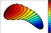
(a) 21 Gauss points

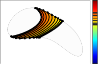
(b) 11 Gauss points

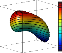
(c) 21 Gauss points

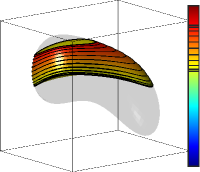
(d) 11 Gauss points

Figure 4: Level sets in the interval $\left[\phi^{\min},\phi^{\max}\right]$ with respect to Gauss integration points, e.g., to numerically confirm Eq. (2.28). In (a) and (c), $\phi^{\min}=\inf\phi\left(\mathchoice{\displaystyle\boldsymbol{x}}{\textstyle\boldsymbol{x}}{\scriptstyle\boldsymbol{x}}{\scriptscriptstyle\boldsymbol{x}}\right)$ and $\phi^{\max}=\sup\phi\left(\mathchoice{\displaystyle\boldsymbol{x}}{\textstyle\boldsymbol{x}}{\scriptstyle\boldsymbol{x}}{\scriptscriptstyle\boldsymbol{x}}\right)$ with $\mathchoice{\displaystyle\boldsymbol{x}}{\textstyle\boldsymbol{x}}{\scriptstyle\boldsymbol{x}}{\scriptscriptstyle\boldsymbol{x}}\in\Omega$, in (b) and (d) $\phi^{\min}$ and $\phi^{\max}$ are user-defined values, see also Section 2.1.

The first important integral theorem is given by the co-area formula [27, 31, 47],

$$\int_{\phi^{\min}}^{\phi^{\max}}\int_{\Gamma^{c}}f\left(\mathchoice{\displaystyle\boldsymbol{x}}{\textstyle\boldsymbol{x}}{\scriptstyle\boldsymbol{x}}{\scriptscriptstyle\boldsymbol{x}}\right)\;\mathrm{d\Gamma}\;\mathrm{d}c=\int_{\Omega}f\left(\mathchoice{\displaystyle\boldsymbol{x}}{\textstyle\boldsymbol{x}}{\scriptstyle\boldsymbol{x}}{\scriptscriptstyle\boldsymbol{x}}\right)\cdot\left\|\nabla\phi\right\|\;\mathrm{d\Omega}.$$ (2.26)

When integrating over the boundary $\partial\Gamma^{c}$ in the level-set interval $\left(\phi^{\min},\;\phi^{\max}\right)$, we find

$$\int_{\phi^{\min}}^{\phi^{\max}}\int_{\partial\Gamma^{c}}f\left(\mathchoice{\displaystyle\boldsymbol{x}}{\textstyle\boldsymbol{x}}{\scriptstyle\boldsymbol{x}}{\scriptscriptstyle\boldsymbol{x}}\right)\;\mathrm{d\partial\Gamma}\;\mathrm{d}c=\int_{\partial\Omega}f\left(\mathchoice{\displaystyle\boldsymbol{x}}{\textstyle\boldsymbol{x}}{\scriptstyle\boldsymbol{x}}{\scriptscriptstyle\boldsymbol{x}}\right)\cdot\left(\mathchoice{\displaystyle\boldsymbol{q}}{\textstyle\boldsymbol{q}}{\scriptstyle\boldsymbol{q}}{\scriptscriptstyle\boldsymbol{q}}\cdot\mathchoice{\displaystyle\boldsymbol{m}}{\textstyle\boldsymbol{m}}{\scriptstyle\boldsymbol{m}}{\scriptscriptstyle\boldsymbol{m}}\right)\cdot\left\|\nabla\phi\right\|\;\mathrm{d\partial\Omega},$$ (2.27)

which is extended from [29, 27]. Note that on the right hand side, the conormal vectors $\mathchoice{\displaystyle\boldsymbol{q}}{\textstyle\boldsymbol{q}}{\scriptstyle\boldsymbol{q}}{\scriptscriptstyle\boldsymbol{q}}$ with respect to $\Gamma^{c}$ as well as the normal vectors $\mathchoice{\displaystyle\boldsymbol{m}}{\textstyle\boldsymbol{m}}{\scriptstyle\boldsymbol{m}}{\scriptscriptstyle\boldsymbol{m}}$ on $\partial\Omega$ are involved. The integral over the level-set interval on the left hand side of Eq. (2.26) may also be evaluated numerically, e.g., using Gauss quadrature,

$$\int_{\phi^{\min}}^{\phi^{\max}}\int_{\Gamma^{c}}f\left(\mathchoice{\displaystyle\boldsymbol{x}}{\textstyle\boldsymbol{x}}{\scriptstyle\boldsymbol{x}}{\scriptscriptstyle\boldsymbol{x}}\right)\;\mathrm{d\Gamma}\;\mathrm{d}c\approx\sum_{i}w_{i}\cdot\int_{\Gamma^{c_{i}}}f\left(\mathchoice{\displaystyle\boldsymbol{x}}{\textstyle\boldsymbol{x}}{\scriptstyle\boldsymbol{x}}{\scriptscriptstyle\boldsymbol{x}}\right)\;\mathrm{d\Gamma},$$ (2.28)

where $w_{i}$ are integration weights and $c_{i}$ are selected level-set values according to the employed Gauss rule, see Fig. 4 for an illustrative setup. The analogy of the two situations of either integrating over $\Omega$ on the right hand side of Eq. (2.26) or numerically on selected level sets according to the right hand side of Eq. (2.28) carries over to either formulating BVPs simultaneously for all level sets in a bulk domain or considering individual BVPs on selected level sets. In this sense, it is later possible to confirm numerical results (i.e., to compare mechanical quantities) obtained by the proposed Bulk Trace FEM for all level sets in a bulk domain with Surface FEM results obtained on selected level sets (according to some Gauss rule as in Eq. (2.28)).

For one selected level set $\Gamma^{c}$ related to the constant value $c$, a scalar function $w\left(\mathchoice{\displaystyle\boldsymbol{x}}{\textstyle\boldsymbol{x}}{\scriptstyle\boldsymbol{x}}{\scriptscriptstyle\boldsymbol{x}}\right)$ and a vector function $\mathchoice{\displaystyle\boldsymbol{u}}{\textstyle\boldsymbol{u}}{\scriptstyle\boldsymbol{u}}{\scriptscriptstyle\boldsymbol{u}}\left(\mathchoice{\displaystyle\boldsymbol{x}}{\textstyle\boldsymbol{x}}{\scriptstyle\boldsymbol{x}}{\scriptscriptstyle\boldsymbol{x}}\right)$, the following divergence theorem on manifolds is well-known [23, 24],

$$\int_{\Gamma^{c}}w\cdot\mathrm{div}_{\Gamma}\mathchoice{\displaystyle\boldsymbol{u}}{\textstyle\boldsymbol{u}}{\scriptstyle\boldsymbol{u}}{\scriptscriptstyle\boldsymbol{u}}\,\mathrm{d}\Gamma=-\int_{\Gamma^{c}}\nabla^{\Gamma}w\cdot\mathchoice{\displaystyle\boldsymbol{u}}{\textstyle\boldsymbol{u}}{\scriptstyle\boldsymbol{u}}{\scriptscriptstyle\boldsymbol{u}}\,\mathrm{d}\Gamma+\int_{\Gamma^{c}}\varkappa\cdot w\cdot\left(\mathchoice{\displaystyle\boldsymbol{u}}{\textstyle\boldsymbol{u}}{\scriptstyle\boldsymbol{u}}{\scriptscriptstyle\boldsymbol{u}}\cdot\mathchoice{\displaystyle\boldsymbol{n}}{\textstyle\boldsymbol{n}}{\scriptstyle\boldsymbol{n}}{\scriptscriptstyle\boldsymbol{n}}\right)\,\mathrm{d}\Gamma+\int_{\partial\Gamma^{c}}w\cdot\left(\mathchoice{\displaystyle\boldsymbol{u}}{\textstyle\boldsymbol{u}}{\scriptstyle\boldsymbol{u}}{\scriptscriptstyle\boldsymbol{u}}\cdot\mathchoice{\displaystyle\boldsymbol{q}}{\textstyle\boldsymbol{q}}{\scriptstyle\boldsymbol{q}}{\scriptscriptstyle\boldsymbol{q}}\right)\,\mathrm{d}\partial\Gamma,$$ (2.29)

where $\varkappa=\mathrm{div}\mathchoice{\displaystyle\boldsymbol{n}}{\textstyle\boldsymbol{n}}{\scriptstyle\boldsymbol{n}}{\scriptscriptstyle\boldsymbol{n}}=\mathrm{div}_{\Gamma}\mathchoice{\displaystyle\boldsymbol{n}}{\textstyle\boldsymbol{n}}{\scriptstyle\boldsymbol{n}}{\scriptscriptstyle\boldsymbol{n}}$ is the mean curvature. Consequently, when integrating over all level sets and using the co-area formulas from above,

$$\int_{\Omega}w\cdot\mathrm{div}_{\Gamma}\mathchoice{\displaystyle\boldsymbol{u}}{\textstyle\boldsymbol{u}}{\scriptstyle\boldsymbol{u}}{\scriptscriptstyle\boldsymbol{u}}\cdot\left\|\nabla\phi\right\|\,\mathrm{d}\Omega= -\int_{\Omega}\nabla^{\Gamma}w\cdot\mathchoice{\displaystyle\boldsymbol{u}}{\textstyle\boldsymbol{u}}{\scriptstyle\boldsymbol{u}}{\scriptscriptstyle\boldsymbol{u}}\cdot\left\|\nabla\phi\right\|\,\mathrm{d}\Omega+\int_{\Omega}\varkappa\cdot w\cdot\left(\mathchoice{\displaystyle\boldsymbol{u}}{\textstyle\boldsymbol{u}}{\scriptstyle\boldsymbol{u}}{\scriptscriptstyle\boldsymbol{u}}\cdot\mathchoice{\displaystyle\boldsymbol{n}}{\textstyle\boldsymbol{n}}{\scriptstyle\boldsymbol{n}}{\scriptscriptstyle\boldsymbol{n}}\right)\cdot\left\|\nabla\phi\right\|\,\mathrm{d}\Omega$$ (2.30)

$$+\int_{\partial\Omega}w\cdot\left(\mathchoice{\displaystyle\boldsymbol{u}}{\textstyle\boldsymbol{u}}{\scriptstyle\boldsymbol{u}}{\scriptscriptstyle\boldsymbol{u}}\cdot\mathchoice{\displaystyle\boldsymbol{q}}{\textstyle\boldsymbol{q}}{\scriptstyle\boldsymbol{q}}{\scriptscriptstyle\boldsymbol{q}}\right)\cdot\left(\mathchoice{\displaystyle\boldsymbol{q}}{\textstyle\boldsymbol{q}}{\scriptstyle\boldsymbol{q}}{\scriptscriptstyle\boldsymbol{q}}\cdot\mathchoice{\displaystyle\boldsymbol{m}}{\textstyle\boldsymbol{m}}{\scriptstyle\boldsymbol{m}}{\scriptscriptstyle\boldsymbol{m}}\right)\cdot\left\|\nabla\phi\right\|\,\mathrm{d}\partial\Omega.$$

It is noted that $\left(\mathchoice{\displaystyle\boldsymbol{u}}{\textstyle\boldsymbol{u}}{\scriptstyle\boldsymbol{u}}{\scriptscriptstyle\boldsymbol{u}}\cdot\mathchoice{\displaystyle\boldsymbol{q}}{\textstyle\boldsymbol{q}}{\scriptstyle\boldsymbol{q}}{\scriptscriptstyle\boldsymbol{q}}\right)\cdot\left(\mathchoice{\displaystyle\boldsymbol{q}}{\textstyle\boldsymbol{q}}{\scriptstyle\boldsymbol{q}}{\scriptscriptstyle\boldsymbol{q}}\cdot\mathchoice{\displaystyle\boldsymbol{m}}{\textstyle\boldsymbol{m}}{\scriptstyle\boldsymbol{m}}{\scriptscriptstyle\boldsymbol{m}}\right)=\left(\mathchoice{\displaystyle\boldsymbol{u}}{\textstyle\boldsymbol{u}}{\scriptstyle\boldsymbol{u}}{\scriptscriptstyle\boldsymbol{u}}\cdot\left(-\mathchoice{\displaystyle\boldsymbol{q}}{\textstyle\boldsymbol{q}}{\scriptstyle\boldsymbol{q}}{\scriptscriptstyle\boldsymbol{q}}\right)\right)\cdot\left(\left(-\mathchoice{\displaystyle\boldsymbol{q}}{\textstyle\boldsymbol{q}}{\scriptstyle\boldsymbol{q}}{\scriptscriptstyle\boldsymbol{q}}\right)\cdot\mathchoice{\displaystyle\boldsymbol{m}}{\textstyle\boldsymbol{m}}{\scriptstyle\boldsymbol{m}}{\scriptscriptstyle\boldsymbol{m}}\right)$ so that in Eq. (2.30) the sign of $\mathchoice{\displaystyle\boldsymbol{q}}{\textstyle\boldsymbol{q}}{\scriptstyle\boldsymbol{q}}{\scriptscriptstyle\boldsymbol{q}}$, hence, the fact whether the conormal vector points inside or outside of the level sets $\Gamma^{c}$, does not matter. Based on this, one may immediately state the divergence theorem for a tensor function $\mathchoice{\displaystyle\mathbf{A}}{\textstyle\mathbf{A}}{\scriptstyle\mathbf{A}}{\scriptscriptstyle\mathbf{A}}\!\left(\mathchoice{\displaystyle\boldsymbol{x}}{\textstyle\boldsymbol{x}}{\scriptstyle\boldsymbol{x}}{\scriptscriptstyle\boldsymbol{x}}\right)$ as

$$\int_{\Omega}\mathchoice{\displaystyle\boldsymbol{u}}{\textstyle\boldsymbol{u}}{\scriptstyle\boldsymbol{u}}{\scriptscriptstyle\boldsymbol{u}}\cdot\mathrm{div}_{\Gamma}\mathchoice{\displaystyle\mathbf{A}}{\textstyle\mathbf{A}}{\scriptstyle\mathbf{A}}{\scriptscriptstyle\mathbf{A}}\cdot\left\|\nabla\phi\right\|\,\mathrm{d}\Omega= -\int_{\Omega}\left(\nabla^{\Gamma,\mathrm{dir}}\mathchoice{\displaystyle\boldsymbol{u}}{\textstyle\boldsymbol{u}}{\scriptstyle\boldsymbol{u}}{\scriptscriptstyle\boldsymbol{u}}:\mathchoice{\displaystyle\mathbf{A}}{\textstyle\mathbf{A}}{\scriptstyle\mathbf{A}}{\scriptscriptstyle\mathbf{A}}\right)\cdot\left\|\nabla\phi\right\|\,\mathrm{d}\Omega+\int_{\Omega}\varkappa\cdot\mathchoice{\displaystyle\boldsymbol{u}}{\textstyle\boldsymbol{u}}{\scriptstyle\boldsymbol{u}}{\scriptscriptstyle\boldsymbol{u}}\cdot\left(\mathchoice{\displaystyle\mathbf{A}}{\textstyle\mathbf{A}}{\scriptstyle\mathbf{A}}{\scriptscriptstyle\mathbf{A}}\cdot\mathchoice{\displaystyle\boldsymbol{n}}{\textstyle\boldsymbol{n}}{\scriptstyle\boldsymbol{n}}{\scriptscriptstyle\boldsymbol{n}}\right)\cdot\left\|\nabla\phi\right\|\,\mathrm{d}\Omega$$ (2.31)

$$+\int_{\partial\Omega}\mathchoice{\displaystyle\boldsymbol{u}}{\textstyle\boldsymbol{u}}{\scriptstyle\boldsymbol{u}}{\scriptscriptstyle\boldsymbol{u}}\cdot\left(\mathchoice{\displaystyle\mathbf{A}}{\textstyle\mathbf{A}}{\scriptstyle\mathbf{A}}{\scriptscriptstyle\mathbf{A}}\cdot\mathchoice{\displaystyle\boldsymbol{q}}{\textstyle\boldsymbol{q}}{\scriptstyle\boldsymbol{q}}{\scriptscriptstyle\boldsymbol{q}}\right)\cdot\left(\mathchoice{\displaystyle\boldsymbol{q}}{\textstyle\boldsymbol{q}}{\scriptstyle\boldsymbol{q}}{\scriptscriptstyle\boldsymbol{q}}\cdot\mathchoice{\displaystyle\boldsymbol{m}}{\textstyle\boldsymbol{m}}{\scriptstyle\boldsymbol{m}}{\scriptscriptstyle\boldsymbol{m}}\right)\cdot\left\|\nabla\phi\right\|\,\mathrm{d}\partial\Omega,$$

which is later needed for the weak formulation of the mechanical equilibrium in finite strain theory. Note that for in-plane tensor functions with $\mathchoice{\displaystyle\mathbf{A}}{\textstyle\mathbf{A}}{\scriptstyle\mathbf{A}}{\scriptscriptstyle\mathbf{A}}=\mathchoice{\displaystyle\mathbf{p}}{\textstyle\mathbf{p}}{\scriptstyle\mathbf{p}}{\scriptscriptstyle\mathbf{p}}\cdot\mathchoice{\displaystyle\mathbf{A}}{\textstyle\mathbf{A}}{\scriptstyle\mathbf{A}}{\scriptscriptstyle\mathbf{A}}\cdot\mathchoice{\displaystyle\mathbf{p}}{\textstyle\mathbf{p}}{\scriptstyle\mathbf{p}}{\scriptscriptstyle\mathbf{p}}$, the term involving the curvature $\varkappa$ vanishes due to $\mathchoice{\displaystyle\mathbf{A}}{\textstyle\mathbf{A}}{\scriptstyle\mathbf{A}}{\scriptscriptstyle\mathbf{A}}\cdot\mathchoice{\displaystyle\boldsymbol{n}}{\textstyle\boldsymbol{n}}{\scriptstyle\boldsymbol{n}}{\scriptscriptstyle\boldsymbol{n}}=\mathchoice{\displaystyle\boldsymbol{0}}{\textstyle\boldsymbol{0}}{\scriptstyle\boldsymbol{0}}{\scriptscriptstyle\boldsymbol{0}}$. Furthermore, one finds for in-plane tensors that $\nabla^{\Gamma,\mathrm{dir}}\mathchoice{\displaystyle\boldsymbol{u}}{\textstyle\boldsymbol{u}}{\scriptstyle\boldsymbol{u}}{\scriptscriptstyle\boldsymbol{u}}:\mathchoice{\displaystyle\mathbf{A}}{\textstyle\mathbf{A}}{\scriptstyle\mathbf{A}}{\scriptscriptstyle\mathbf{A}}=\nabla^{\Gamma,\mathrm{cov}}\mathchoice{\displaystyle\boldsymbol{u}}{\textstyle\boldsymbol{u}}{\scriptstyle\boldsymbol{u}}{\scriptscriptstyle\boldsymbol{u}}:\mathchoice{\displaystyle\mathbf{A}}{\textstyle\mathbf{A}}{\scriptstyle\mathbf{A}}{\scriptscriptstyle\mathbf{A}}$.

2.5 Invalid combinations of level sets and bulk domains

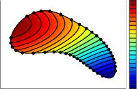
(a) valid

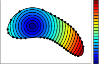
(b) invalid

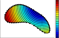
(c) invalid

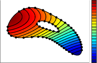
(d) invalid

Figure 5: Valid and invalid combinations of level-set functions $\phi$ and bulk domains $\Omega$.

The simultaneous mechanical modeling and simulation of curved structures on all level sets over a bulk domain requires everywhere a smooth transition of the displacement fields between neighbouring level sets. Most importantly, the topology of neighboring level sets must not change discontinuously in $\Omega$. Combinations which do not lead to smooth variations of the implied level-set geometries $\Gamma^{c}$ in some given bulk domain $\Omega$ may be called invalid. Examples are seen in Fig. 5 where (a) shows a valid situation but (b) to (d) are invalid. In Fig. 5(b), a situation is seen where some level sets feature two end points, however, others are closed and do not feature boundaries $\partial\Gamma^{c}$. This is the result of a local maximum of the level-set function within the domain $\Omega$ which, hence, must be excluded. Fig. 5(c) shows a situation where some level sets feature two end points, however, others three or four which results from the opposite curvature of $\partial\Omega$ and $\Gamma^{c}$ on the lower side of the bulk domain. In Fig. 5(d), the level-set function is identical to the valid situation in Fig. 5(a), however, there is now a hole inside the bulk domain $\Omega$, so that the number of end points of the level sets also varies inside $\Omega$ being invalid.

Note that in all invalid cases, it is the interplay between the (smooth) geometry of the bulk domain $\Omega$ and the (smooth) level-set function $\phi$ which generated these invalid scenarios. Obviously, local extreme values of $\phi$ inside $\Omega$ have to be excluded (hence, $\inf\phi$ and $\sup\phi$ must be on the boundary $\partial\Omega$). Additional requirements are related to the curvature of $\phi$ near the boundary $\partial\Omega$. The validity of level sets with respect to bulk domains has also been discussed in [27]. Herein, rather than (re-)formulating mathematically sound requirements for $\phi$ and $\Omega$ we rather state that only combinations of $\phi$ and $\Omega$ are allowed where all level sets vary smoothly inside $\Omega$, enabling smooth mechanical fields.

Figure 6: Invalid combinations of $\phi$ and $\Omega$ may still be considered if the bulk domain is reduced to certain sub-domains (related to certain intervals of the level-set function) in which the topology does not change, i.e., where the geometries of $\Gamma^{c}$ vary smoothly (regions with individual gray scales).

It is also noteworthy that in invalid cases, one may still pose mechanically meaningful BVPs over sub-domains of $\Omega$ related to individual intervals of the level-set function $\phi$ where the level sets vary smoothly and then assess all sub-domains successively. Of course, in this case, one needs to generate individual meshes in each of the sub-domains to carry out the numerical analyses (according to Section 4). In Fig. 5, such sub-domains (related to certain intervals of the level-set function) are highlighted, related to the situations shown in Fig. 5, using different gray scales. This is related to the alternative definition of bulk domains via prescribed values for $\phi^{\min}$ and $\phi^{\max}$ as described in Section 2.1. It is noted that the rather strong assumptions on the validity of level sets in bulk domains are largely alleviated when the bulk domain itself is equipped with mechanical properties as discussed in Section 3.7, leading to a new class of anisotropic material models for continuously embedded sub-structures in bulk domains.

3 Mechanical setup in finite strain theory

3.1 Undeformed and deformed configurations

In finite strain or large displacement theory, we distinguish an undeformed material configuration and a deformed spatial configuration. With configuration we refer to all level sets of a level-set function over some $d$-dimensional bulk domain. As usual in finite strain theory, we use upper case letters for quantities in the undeformed configuration and lower case letters for the deformed configuration.

Let the undeformed bulk domain be $\Omega_{\mathchoice{\displaystyle\boldsymbol{X}}{\textstyle\boldsymbol{X}}{\scriptstyle\boldsymbol{X}}{\scriptscriptstyle\boldsymbol{X}}}$ and the level-set function $\phi\left(\mathchoice{\displaystyle\boldsymbol{X}}{\textstyle\boldsymbol{X}}{\scriptstyle\boldsymbol{X}}{\scriptscriptstyle\boldsymbol{X}}\right):\Omega_{\mathchoice{\displaystyle\boldsymbol{X}}{\textstyle\boldsymbol{X}}{\scriptstyle\boldsymbol{X}}{\scriptscriptstyle\boldsymbol{X}}}\rightarrow\mathbb{R}$. Then, the individual undeformed domains of interest $\Gamma_{\!\!\mathchoice{\displaystyle\boldsymbol{X}}{\textstyle\boldsymbol{X}}{\scriptstyle\boldsymbol{X}}{\scriptscriptstyle\boldsymbol{X}}}^{c}$ (being the set of membranes or ropes simultaneously considered) are each related to constant level-set values,

$$\Gamma_{\!\!\mathchoice{\displaystyle\boldsymbol{X}}{\textstyle\boldsymbol{X}}{\scriptstyle\boldsymbol{X}}{\scriptscriptstyle\boldsymbol{X}}}^{c}=\left\{\mathchoice{\displaystyle\boldsymbol{X}}{\textstyle\boldsymbol{X}}{\scriptstyle\boldsymbol{X}}{\scriptscriptstyle\boldsymbol{X}}\in\Omega_{\mathchoice{\displaystyle\boldsymbol{X}}{\textstyle\boldsymbol{X}}{\scriptstyle\boldsymbol{X}}{\scriptscriptstyle\boldsymbol{X}}}:\,\phi(\mathchoice{\displaystyle\boldsymbol{X}}{\textstyle\boldsymbol{X}}{\scriptstyle\boldsymbol{X}}{\scriptscriptstyle\boldsymbol{X}})=c\right\},\,c\in\left(\phi^{\min},\;\phi^{\max}\right),$$ (3.1)

analogously to Eq. (2.1). One may now define an individual boundary value problem for every $\Gamma_{\!\!\mathchoice{\displaystyle\boldsymbol{X}}{\textstyle\boldsymbol{X}}{\scriptstyle\boldsymbol{X}}{\scriptscriptstyle\boldsymbol{X}}}^{c}$ and determine the individual displacement field $\mathchoice{\displaystyle\boldsymbol{u}}{\textstyle\boldsymbol{u}}{\scriptstyle\boldsymbol{u}}{\scriptscriptstyle\boldsymbol{u}}\left(\mathchoice{\displaystyle\boldsymbol{X}}{\textstyle\boldsymbol{X}}{\scriptstyle\boldsymbol{X}}{\scriptscriptstyle\boldsymbol{X}}\right)$ of every level set [36]. However, the displacements between neighboring level sets (usually) vary smoothly, cf. Section 2.5, so that we rather seek the displacement field of all level sets at once. That is, the deformed bulk domain

$$\Omega_{\mathchoice{\displaystyle\boldsymbol{x}}{\textstyle\boldsymbol{x}}{\scriptstyle\boldsymbol{x}}{\scriptscriptstyle\boldsymbol{x}}}=\left\{\mathchoice{\displaystyle\boldsymbol{x}}{\textstyle\boldsymbol{x}}{\scriptstyle\boldsymbol{x}}{\scriptscriptstyle\boldsymbol{x}}=\mathchoice{\displaystyle\boldsymbol{X}}{\textstyle\boldsymbol{X}}{\scriptstyle\boldsymbol{X}}{\scriptscriptstyle\boldsymbol{X}}+\mathchoice{\displaystyle\boldsymbol{u}}{\textstyle\boldsymbol{u}}{\scriptstyle\boldsymbol{u}}{\scriptscriptstyle\boldsymbol{u}}\left(\mathchoice{\displaystyle\boldsymbol{X}}{\textstyle\boldsymbol{X}}{\scriptstyle\boldsymbol{X}}{\scriptscriptstyle\boldsymbol{X}}\right),\mathchoice{\displaystyle\boldsymbol{X}}{\textstyle\boldsymbol{X}}{\scriptstyle\boldsymbol{X}}{\scriptscriptstyle\boldsymbol{X}}\in\Omega_{\mathchoice{\displaystyle\boldsymbol{X}}{\textstyle\boldsymbol{X}}{\scriptstyle\boldsymbol{X}}{\scriptscriptstyle\boldsymbol{X}}}\right\}$$

is sought such that

$$\Gamma_{\!\!\mathchoice{\displaystyle\boldsymbol{x}}{\textstyle\boldsymbol{x}}{\scriptstyle\boldsymbol{x}}{\scriptscriptstyle\boldsymbol{x}}}^{c}=\left\{\mathchoice{\displaystyle\boldsymbol{x}}{\textstyle\boldsymbol{x}}{\scriptstyle\boldsymbol{x}}{\scriptscriptstyle\boldsymbol{x}}\in\Omega_{\mathchoice{\displaystyle\boldsymbol{x}}{\textstyle\boldsymbol{x}}{\scriptstyle\boldsymbol{x}}{\scriptscriptstyle\boldsymbol{x}}}:\,\phi(\mathchoice{\displaystyle\boldsymbol{x}}{\textstyle\boldsymbol{x}}{\scriptstyle\boldsymbol{x}}{\scriptscriptstyle\boldsymbol{x}})=c\right\},\,c\in\left(\phi^{\min},\;\phi^{\max}\right)$$

are the deformed structures. Illustratively, plotting selected level sets of $\phi\left(\mathchoice{\displaystyle\boldsymbol{X}}{\textstyle\boldsymbol{X}}{\scriptstyle\boldsymbol{X}}{\scriptscriptstyle\boldsymbol{X}}\right)$ in $\Omega_{\mathchoice{\displaystyle\boldsymbol{X}}{\textstyle\boldsymbol{X}}{\scriptstyle\boldsymbol{X}}{\scriptscriptstyle\boldsymbol{X}}}$ shows some undeformed structures whereas plotting the same level sets of $\phi\left(\mathchoice{\displaystyle\boldsymbol{x}}{\textstyle\boldsymbol{x}}{\scriptstyle\boldsymbol{x}}{\scriptscriptstyle\boldsymbol{x}}\right)$ in $\Omega_{\mathchoice{\displaystyle\boldsymbol{x}}{\textstyle\boldsymbol{x}}{\scriptstyle\boldsymbol{x}}{\scriptscriptstyle\boldsymbol{x}}}$ represents the resulting deformed structures, see Fig. 7.

(a) situation in 2D

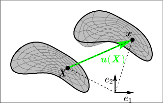
(b) mesh in 2D

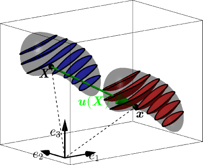
(c) situation in 3D

Figure 7: Undeformed material configuration and deformed spatial configuration in two and three dimensions. The bulk domains $\Omega_{\mathchoice{\displaystyle\boldsymbol{X}}{\textstyle\boldsymbol{X}}{\scriptstyle\boldsymbol{X}}{\scriptscriptstyle\boldsymbol{X}}}$ and $\Omega_{\mathchoice{\displaystyle\boldsymbol{x}}{\textstyle\boldsymbol{x}}{\scriptstyle\boldsymbol{x}}{\scriptscriptstyle\boldsymbol{x}}}$ are shown in gray. The undeformed level sets $\Gamma_{\!\!\mathchoice{\displaystyle\boldsymbol{X}}{\textstyle\boldsymbol{X}}{\scriptstyle\boldsymbol{X}}{\scriptscriptstyle\boldsymbol{X}}}^{c}$ are blue and the deformed level sets $\Gamma_{\!\!\mathchoice{\displaystyle\boldsymbol{x}}{\textstyle\boldsymbol{x}}{\scriptstyle\boldsymbol{x}}{\scriptscriptstyle\boldsymbol{x}}}^{c}$ are red. In (b), the corresponding meshes in the bulk domains $\Omega_{\mathchoice{\displaystyle\boldsymbol{X}}{\textstyle\boldsymbol{X}}{\scriptstyle\boldsymbol{X}}{\scriptscriptstyle\boldsymbol{X}}}$ and $\Omega_{\mathchoice{\displaystyle\boldsymbol{x}}{\textstyle\boldsymbol{x}}{\scriptstyle\boldsymbol{x}}{\scriptscriptstyle\boldsymbol{x}}}$, as used for the approximation of the displacement field $\mathchoice{\displaystyle\boldsymbol{u}}{\textstyle\boldsymbol{u}}{\scriptstyle\boldsymbol{u}}{\scriptscriptstyle\boldsymbol{u}}\left(\mathchoice{\displaystyle\boldsymbol{X}}{\textstyle\boldsymbol{X}}{\scriptstyle\boldsymbol{X}}{\scriptscriptstyle\boldsymbol{X}}\right)$, are depicted.

The geometric quantities and differential operators formulated in Section 2 extend straightforwardly to the mechanical setup outlined here with only small distinctions in the notation to specify whether these quantities relate to the undeformed or deformed situation. They are shortly summarized in Table 1. The bulk domains $\Omega_{\mathchoice{\displaystyle\boldsymbol{X}}{\textstyle\boldsymbol{X}}{\scriptstyle\boldsymbol{X}}{\scriptscriptstyle\boldsymbol{X}}}$ and $\Omega_{\mathchoice{\displaystyle\boldsymbol{x}}{\textstyle\boldsymbol{x}}{\scriptstyle\boldsymbol{x}}{\scriptscriptstyle\boldsymbol{x}}}$ feature boundaries $\partial\Omega_{\mathchoice{\displaystyle\boldsymbol{X}}{\textstyle\boldsymbol{X}}{\scriptstyle\boldsymbol{X}}{\scriptscriptstyle\boldsymbol{X}}}$ and $\partial\Omega_{\mathchoice{\displaystyle\boldsymbol{x}}{\textstyle\boldsymbol{x}}{\scriptstyle\boldsymbol{x}}{\scriptscriptstyle\boldsymbol{x}}}$ with unit normal vectors $\mathchoice{\displaystyle\boldsymbol{M}}{\textstyle\boldsymbol{M}}{\scriptstyle\boldsymbol{M}}{\scriptscriptstyle\boldsymbol{M}}$ and $\mathchoice{\displaystyle\boldsymbol{m}}{\textstyle\boldsymbol{m}}{\scriptstyle\boldsymbol{m}}{\scriptscriptstyle\boldsymbol{m}}$, respectively. $\mathchoice{\displaystyle\boldsymbol{N}}{\textstyle\boldsymbol{N}}{\scriptstyle\boldsymbol{N}}{\scriptscriptstyle\boldsymbol{N}}$ and $\mathchoice{\displaystyle\boldsymbol{n}}{\textstyle\boldsymbol{n}}{\scriptstyle\boldsymbol{n}}{\scriptscriptstyle\boldsymbol{n}}$ are the respective unit normal vectors on the level sets $\Gamma_{\!\!\mathchoice{\displaystyle\boldsymbol{X}}{\textstyle\boldsymbol{X}}{\scriptstyle\boldsymbol{X}}{\scriptscriptstyle\boldsymbol{X}}}^{c}$ and $\Gamma_{\!\!\mathchoice{\displaystyle\boldsymbol{x}}{\textstyle\boldsymbol{x}}{\scriptstyle\boldsymbol{x}}{\scriptscriptstyle\boldsymbol{x}}}^{c}$ in the bulk domains, and $\mathchoice{\displaystyle\boldsymbol{Q}}{\textstyle\boldsymbol{Q}}{\scriptstyle\boldsymbol{Q}}{\scriptscriptstyle\boldsymbol{Q}}$ and $\mathchoice{\displaystyle\boldsymbol{q}}{\textstyle\boldsymbol{q}}{\scriptstyle\boldsymbol{q}}{\scriptscriptstyle\boldsymbol{q}}$ the conormal vectors on the boundaries.

	undef. material configuration	def. spatial configuration
bulk domain	$\begin{array}[]{l}\Omega_{\mathchoice{\displaystyle\boldsymbol{X}}{\textstyle\boldsymbol{X}}{\scriptstyle\boldsymbol{X}}{\scriptscriptstyle\boldsymbol{X}}}\subset\mathbb{R}^{d}\\ \text{with boundary }\partial\Omega_{\mathchoice{\displaystyle\boldsymbol{X}}{\textstyle\boldsymbol{X}}{\scriptstyle\boldsymbol{X}}{\scriptscriptstyle\boldsymbol{X}}}\end{array}$	$\begin{array}[]{l}\Omega_{\mathchoice{\displaystyle\boldsymbol{x}}{\textstyle\boldsymbol{x}}{\scriptstyle\boldsymbol{x}}{\scriptscriptstyle\boldsymbol{x}}}=\left\{\mathchoice{\displaystyle\boldsymbol{x}}{\textstyle\boldsymbol{x}}{\scriptstyle\boldsymbol{x}}{\scriptscriptstyle\boldsymbol{x}}=\mathchoice{\displaystyle\boldsymbol{X}}{\textstyle\boldsymbol{X}}{\scriptstyle\boldsymbol{X}}{\scriptscriptstyle\boldsymbol{X}}+\mathchoice{\displaystyle\boldsymbol{u}}{\textstyle\boldsymbol{u}}{\scriptstyle\boldsymbol{u}}{\scriptscriptstyle\boldsymbol{u}}\left(\mathchoice{\displaystyle\boldsymbol{X}}{\textstyle\boldsymbol{X}}{\scriptstyle\boldsymbol{X}}{\scriptscriptstyle\boldsymbol{X}}\right),\mathchoice{\displaystyle\boldsymbol{X}}{\textstyle\boldsymbol{X}}{\scriptstyle\boldsymbol{X}}{\scriptscriptstyle\boldsymbol{X}}\in\Omega_{\mathchoice{\displaystyle\boldsymbol{X}}{\textstyle\boldsymbol{X}}{\scriptstyle\boldsymbol{X}}{\scriptscriptstyle\boldsymbol{X}}}\right\}\\ \text{with boundary }\partial\Omega_{\mathchoice{\displaystyle\boldsymbol{x}}{\textstyle\boldsymbol{x}}{\scriptstyle\boldsymbol{x}}{\scriptscriptstyle\boldsymbol{x}}}\end{array}$
level-set function	$\phi\left(\mathchoice{\displaystyle\boldsymbol{X}}{\textstyle\boldsymbol{X}}{\scriptstyle\boldsymbol{X}}{\scriptscriptstyle\boldsymbol{X}}\right),\;\mathchoice{\displaystyle\boldsymbol{X}}{\textstyle\boldsymbol{X}}{\scriptstyle\boldsymbol{X}}{\scriptscriptstyle\boldsymbol{X}}\in\Omega_{\mathchoice{\displaystyle\boldsymbol{X}}{\textstyle\boldsymbol{X}}{\scriptstyle\boldsymbol{X}}{\scriptscriptstyle\boldsymbol{X}}}$	$\phi\left(\mathchoice{\displaystyle\boldsymbol{x}}{\textstyle\boldsymbol{x}}{\scriptstyle\boldsymbol{x}}{\scriptscriptstyle\boldsymbol{x}}\right),\;\mathchoice{\displaystyle\boldsymbol{x}}{\textstyle\boldsymbol{x}}{\scriptstyle\boldsymbol{x}}{\scriptscriptstyle\boldsymbol{x}}\in\Omega_{\mathchoice{\displaystyle\boldsymbol{x}}{\textstyle\boldsymbol{x}}{\scriptstyle\boldsymbol{x}}{\scriptscriptstyle\boldsymbol{x}}}$
$\begin{array}[]{l}\text{level sets}\\ \text{(=curved structures)}\end{array}$	$\begin{array}[]{l}\Gamma_{\!\!\mathchoice{\displaystyle\boldsymbol{X}}{\textstyle\boldsymbol{X}}{\scriptstyle\boldsymbol{X}}{\scriptscriptstyle\boldsymbol{X}}}^{c}=\{\mathchoice{\displaystyle\boldsymbol{X}}{\textstyle\boldsymbol{X}}{\scriptstyle\boldsymbol{X}}{\scriptscriptstyle\boldsymbol{X}}\in\Omega_{\mathchoice{\displaystyle\boldsymbol{X}}{\textstyle\boldsymbol{X}}{\scriptstyle\boldsymbol{X}}{\scriptscriptstyle\boldsymbol{X}}}:\phi(\mathchoice{\displaystyle\boldsymbol{X}}{\textstyle\boldsymbol{X}}{\scriptstyle\boldsymbol{X}}{\scriptscriptstyle\boldsymbol{X}})=c\},\\ c\in\left(\phi^{\min},\;\phi^{\max}\right)\end{array}$	$\begin{array}[]{l}\Gamma_{\!\!\mathchoice{\displaystyle\boldsymbol{x}}{\textstyle\boldsymbol{x}}{\scriptstyle\boldsymbol{x}}{\scriptscriptstyle\boldsymbol{x}}}^{c}=\{\mathchoice{\displaystyle\boldsymbol{x}}{\textstyle\boldsymbol{x}}{\scriptstyle\boldsymbol{x}}{\scriptscriptstyle\boldsymbol{x}}\in\Omega_{\mathchoice{\displaystyle\boldsymbol{x}}{\textstyle\boldsymbol{x}}{\scriptstyle\boldsymbol{x}}{\scriptscriptstyle\boldsymbol{x}}}:\phi(\mathchoice{\displaystyle\boldsymbol{x}}{\textstyle\boldsymbol{x}}{\scriptstyle\boldsymbol{x}}{\scriptscriptstyle\boldsymbol{x}})=c\},\\ c\in\left(\phi^{\min},\;\phi^{\max}\right)\end{array}$
$\begin{array}[]{l}\text{unit normal vectors}\\ \text{w.r.t. bulk domain}\end{array}$	$\mathchoice{\displaystyle\boldsymbol{M}}{\textstyle\boldsymbol{M}}{\scriptstyle\boldsymbol{M}}{\scriptscriptstyle\boldsymbol{M}}\;\text{on}\;\partial\Omega_{\mathchoice{\displaystyle\boldsymbol{X}}{\textstyle\boldsymbol{X}}{\scriptstyle\boldsymbol{X}}{\scriptscriptstyle\boldsymbol{X}}}$	$\mathchoice{\displaystyle\boldsymbol{m}}{\textstyle\boldsymbol{m}}{\scriptstyle\boldsymbol{m}}{\scriptscriptstyle\boldsymbol{m}}\;\text{on}\;\partial\Omega_{\mathchoice{\displaystyle\boldsymbol{x}}{\textstyle\boldsymbol{x}}{\scriptstyle\boldsymbol{x}}{\scriptscriptstyle\boldsymbol{x}}}$
bulk def. gradient	$\mathchoice{\displaystyle\mathbf{F}}{\textstyle\mathbf{F}}{\scriptstyle\mathbf{F}}{\scriptscriptstyle\mathbf{F}}_{\Omega}=\nabla_{\mathchoice{\displaystyle\boldsymbol{X}}{\textstyle\boldsymbol{X}}{\scriptstyle\boldsymbol{X}}{\scriptscriptstyle\boldsymbol{X}}}\mathchoice{\displaystyle\boldsymbol{x}}{\textstyle\boldsymbol{x}}{\scriptstyle\boldsymbol{x}}{\scriptscriptstyle\boldsymbol{x}}\left(\mathchoice{\displaystyle\boldsymbol{X}}{\textstyle\boldsymbol{X}}{\scriptstyle\boldsymbol{X}}{\scriptscriptstyle\boldsymbol{X}}\right)=\mathchoice{\displaystyle\mathbf{I}}{\textstyle\mathbf{I}}{\scriptstyle\mathbf{I}}{\scriptscriptstyle\mathbf{I}}+\nabla_{\mathchoice{\displaystyle\boldsymbol{X}}{\textstyle\boldsymbol{X}}{\scriptstyle\boldsymbol{X}}{\scriptscriptstyle\boldsymbol{X}}}\mathchoice{\displaystyle\boldsymbol{u}}{\textstyle\boldsymbol{u}}{\scriptstyle\boldsymbol{u}}{\scriptscriptstyle\boldsymbol{u}}\left(\mathchoice{\displaystyle\boldsymbol{X}}{\textstyle\boldsymbol{X}}{\scriptstyle\boldsymbol{X}}{\scriptscriptstyle\boldsymbol{X}}\right)$
$\begin{array}[]{l}\text{unit normal vectors}\\ \text{w.r.t. level sets}\end{array}$	$\mathchoice{\displaystyle\boldsymbol{N}}{\textstyle\boldsymbol{N}}{\scriptstyle\boldsymbol{N}}{\scriptscriptstyle\boldsymbol{N}}=\frac{\mathchoice{\displaystyle\boldsymbol{N}}{\textstyle\boldsymbol{N}}{\scriptstyle\boldsymbol{N}}{\scriptscriptstyle\boldsymbol{N}}^{\star}}{\left\|\mathchoice{\displaystyle\boldsymbol{N}}{\textstyle\boldsymbol{N}}{\scriptstyle\boldsymbol{N}}{\scriptscriptstyle\boldsymbol{N}}^{\star}\right\|},\;\mathchoice{\displaystyle\boldsymbol{N}}{\textstyle\boldsymbol{N}}{\scriptstyle\boldsymbol{N}}{\scriptscriptstyle\boldsymbol{N}}^{\star}=\nabla_{\mathchoice{\displaystyle\boldsymbol{X}}{\textstyle\boldsymbol{X}}{\scriptstyle\boldsymbol{X}}{\scriptscriptstyle\boldsymbol{X}}}\phi$	$\mathchoice{\displaystyle\boldsymbol{n}}{\textstyle\boldsymbol{n}}{\scriptstyle\boldsymbol{n}}{\scriptscriptstyle\boldsymbol{n}}=\frac{\mathchoice{\displaystyle\boldsymbol{n}}{\textstyle\boldsymbol{n}}{\scriptstyle\boldsymbol{n}}{\scriptscriptstyle\boldsymbol{n}}^{\star}}{\left\|\mathchoice{\displaystyle\boldsymbol{n}}{\textstyle\boldsymbol{n}}{\scriptstyle\boldsymbol{n}}{\scriptscriptstyle\boldsymbol{n}}^{\star}\right\|},\;\mathchoice{\displaystyle\boldsymbol{n}}{\textstyle\boldsymbol{n}}{\scriptstyle\boldsymbol{n}}{\scriptscriptstyle\boldsymbol{n}}^{\star}=\mathchoice{\displaystyle\mathbf{F}}{\textstyle\mathbf{F}}{\scriptstyle\mathbf{F}}{\scriptscriptstyle\mathbf{F}}_{\Omega}^{-\mathrm{T}}\cdot\mathchoice{\displaystyle\boldsymbol{N}}{\textstyle\boldsymbol{N}}{\scriptstyle\boldsymbol{N}}{\scriptscriptstyle\boldsymbol{N}}^{\star}$
projectors	$\mathchoice{\displaystyle\mathbf{P}}{\textstyle\mathbf{P}}{\scriptstyle\mathbf{P}}{\scriptscriptstyle\mathbf{P}}=\mathchoice{\displaystyle\mathbf{I}}{\textstyle\mathbf{I}}{\scriptstyle\mathbf{I}}{\scriptscriptstyle\mathbf{I}}-\mathchoice{\displaystyle\boldsymbol{N}}{\textstyle\boldsymbol{N}}{\scriptstyle\boldsymbol{N}}{\scriptscriptstyle\boldsymbol{N}}\otimes\mathchoice{\displaystyle\boldsymbol{N}}{\textstyle\boldsymbol{N}}{\scriptstyle\boldsymbol{N}}{\scriptscriptstyle\boldsymbol{N}}$	$\mathchoice{\displaystyle\mathbf{p}}{\textstyle\mathbf{p}}{\scriptstyle\mathbf{p}}{\scriptscriptstyle\mathbf{p}}=\mathchoice{\displaystyle\mathbf{I}}{\textstyle\mathbf{I}}{\scriptstyle\mathbf{I}}{\scriptscriptstyle\mathbf{I}}-\mathchoice{\displaystyle\boldsymbol{n}}{\textstyle\boldsymbol{n}}{\scriptstyle\boldsymbol{n}}{\scriptscriptstyle\boldsymbol{n}}\otimes\mathchoice{\displaystyle\boldsymbol{n}}{\textstyle\boldsymbol{n}}{\scriptstyle\boldsymbol{n}}{\scriptscriptstyle\boldsymbol{n}}$
$\begin{array}[]{l}\text{unit conormal}\\ \text{vectors in }\mathbb{R}^{2}\end{array}$	$\mathchoice{\displaystyle\boldsymbol{Q}}{\textstyle\boldsymbol{Q}}{\scriptstyle\boldsymbol{Q}}{\scriptscriptstyle\boldsymbol{Q}}=\left[\begin{array}[]{c}Q_{x}\\ Q_{y}\end{array}\right]=\left[\begin{array}[]{c}-N_{y}\\ N_{x}\end{array}\right]$	$\mathchoice{\displaystyle\boldsymbol{q}}{\textstyle\boldsymbol{q}}{\scriptstyle\boldsymbol{q}}{\scriptscriptstyle\boldsymbol{q}}=\left[\begin{array}[]{c}q_{x}\\ q_{y}\end{array}\right]=\left[\begin{array}[]{c}-n_{y}\\ n_{x}\end{array}\right]$
$\begin{array}[]{l}\text{unit conormal}\\ \text{vectors in }\mathbb{R}^{3}\end{array}$	$\mathchoice{\displaystyle\boldsymbol{Q}}{\textstyle\boldsymbol{Q}}{\scriptstyle\boldsymbol{Q}}{\scriptscriptstyle\boldsymbol{Q}}=\frac{\mathchoice{\displaystyle\boldsymbol{Q}}{\textstyle\boldsymbol{Q}}{\scriptstyle\boldsymbol{Q}}{\scriptscriptstyle\boldsymbol{Q}}^{\star}}{\left\|\mathchoice{\displaystyle\boldsymbol{Q}}{\textstyle\boldsymbol{Q}}{\scriptstyle\boldsymbol{Q}}{\scriptscriptstyle\boldsymbol{Q}}^{\star}\right\|},\;\mathchoice{\displaystyle\boldsymbol{Q}}{\textstyle\boldsymbol{Q}}{\scriptstyle\boldsymbol{Q}}{\scriptscriptstyle\boldsymbol{Q}}^{\star}=\mathchoice{\displaystyle\boldsymbol{N}}{\textstyle\boldsymbol{N}}{\scriptstyle\boldsymbol{N}}{\scriptscriptstyle\boldsymbol{N}}\times\mathchoice{\displaystyle\boldsymbol{M}}{\textstyle\boldsymbol{M}}{\scriptstyle\boldsymbol{M}}{\scriptscriptstyle\boldsymbol{M}}\times\mathchoice{\displaystyle\boldsymbol{N}}{\textstyle\boldsymbol{N}}{\scriptstyle\boldsymbol{N}}{\scriptscriptstyle\boldsymbol{N}}$	$\mathchoice{\displaystyle\boldsymbol{q}}{\textstyle\boldsymbol{q}}{\scriptstyle\boldsymbol{q}}{\scriptscriptstyle\boldsymbol{q}}=\frac{\mathchoice{\displaystyle\boldsymbol{q}}{\textstyle\boldsymbol{q}}{\scriptstyle\boldsymbol{q}}{\scriptscriptstyle\boldsymbol{q}}^{\star}}{\left\|\mathchoice{\displaystyle\boldsymbol{q}}{\textstyle\boldsymbol{q}}{\scriptstyle\boldsymbol{q}}{\scriptscriptstyle\boldsymbol{q}}^{\star}\right\|},\;\mathchoice{\displaystyle\boldsymbol{q}}{\textstyle\boldsymbol{q}}{\scriptstyle\boldsymbol{q}}{\scriptscriptstyle\boldsymbol{q}}^{\star}=\mathchoice{\displaystyle\boldsymbol{n}}{\textstyle\boldsymbol{n}}{\scriptstyle\boldsymbol{n}}{\scriptscriptstyle\boldsymbol{n}}\times\mathchoice{\displaystyle\boldsymbol{m}}{\textstyle\boldsymbol{m}}{\scriptstyle\boldsymbol{m}}{\scriptscriptstyle\boldsymbol{m}}\times\mathchoice{\displaystyle\boldsymbol{n}}{\textstyle\boldsymbol{n}}{\scriptstyle\boldsymbol{n}}{\scriptscriptstyle\boldsymbol{n}}$
line/area stretch	$\Lambda=\frac{\left\|\mathchoice{\displaystyle\boldsymbol{n}}{\textstyle\boldsymbol{n}}{\scriptstyle\boldsymbol{n}}{\scriptscriptstyle\boldsymbol{n}}^{\star}\right\|}{\left\|\mathchoice{\displaystyle\boldsymbol{N}}{\textstyle\boldsymbol{N}}{\scriptstyle\boldsymbol{N}}{\scriptscriptstyle\boldsymbol{N}}^{\star}\right\|}\cdot\det\mathchoice{\displaystyle\mathbf{F}}{\textstyle\mathbf{F}}{\scriptstyle\mathbf{F}}{\scriptscriptstyle\mathbf{F}}_{\Omega}$
$\begin{array}[]{l}\text{surface gradient}\\ \text{of scalar function}\end{array}$	$\nabla_{\mathchoice{\displaystyle\boldsymbol{X}}{\textstyle\boldsymbol{X}}{\scriptstyle\boldsymbol{X}}{\scriptscriptstyle\boldsymbol{X}}}^{\Gamma}f=\mathchoice{\displaystyle\mathbf{P}}{\textstyle\mathbf{P}}{\scriptstyle\mathbf{P}}{\scriptscriptstyle\mathbf{P}}\cdot\nabla_{\mathchoice{\displaystyle\boldsymbol{X}}{\textstyle\boldsymbol{X}}{\scriptstyle\boldsymbol{X}}{\scriptscriptstyle\boldsymbol{X}}}f$	$\nabla_{\mathchoice{\displaystyle\boldsymbol{x}}{\textstyle\boldsymbol{x}}{\scriptstyle\boldsymbol{x}}{\scriptscriptstyle\boldsymbol{x}}}^{\Gamma}f=\mathchoice{\displaystyle\mathbf{p}}{\textstyle\mathbf{p}}{\scriptstyle\mathbf{p}}{\scriptscriptstyle\mathbf{p}}\cdot\nabla_{\mathchoice{\displaystyle\boldsymbol{x}}{\textstyle\boldsymbol{x}}{\scriptstyle\boldsymbol{x}}{\scriptscriptstyle\boldsymbol{x}}}f$
$\begin{array}[]{l}\text{dir. surface gradient}\\ \text{of vector function}\end{array}$	$\nabla_{\mathchoice{\displaystyle\boldsymbol{X}}{\textstyle\boldsymbol{X}}{\scriptstyle\boldsymbol{X}}{\scriptscriptstyle\boldsymbol{X}}}^{\Gamma,\mathrm{dir}}\mathchoice{\displaystyle\boldsymbol{u}}{\textstyle\boldsymbol{u}}{\scriptstyle\boldsymbol{u}}{\scriptscriptstyle\boldsymbol{u}}=\nabla_{\mathchoice{\displaystyle\boldsymbol{X}}{\textstyle\boldsymbol{X}}{\scriptstyle\boldsymbol{X}}{\scriptscriptstyle\boldsymbol{X}}}\mathchoice{\displaystyle\boldsymbol{u}}{\textstyle\boldsymbol{u}}{\scriptstyle\boldsymbol{u}}{\scriptscriptstyle\boldsymbol{u}}\cdot\mathchoice{\displaystyle\mathbf{P}}{\textstyle\mathbf{P}}{\scriptstyle\mathbf{P}}{\scriptscriptstyle\mathbf{P}}$	$\nabla_{\mathchoice{\displaystyle\boldsymbol{x}}{\textstyle\boldsymbol{x}}{\scriptstyle\boldsymbol{x}}{\scriptscriptstyle\boldsymbol{x}}}^{\Gamma,\mathrm{dir}}\mathchoice{\displaystyle\boldsymbol{u}}{\textstyle\boldsymbol{u}}{\scriptstyle\boldsymbol{u}}{\scriptscriptstyle\boldsymbol{u}}=\nabla_{\mathchoice{\displaystyle\boldsymbol{x}}{\textstyle\boldsymbol{x}}{\scriptstyle\boldsymbol{x}}{\scriptscriptstyle\boldsymbol{x}}}\mathchoice{\displaystyle\boldsymbol{u}}{\textstyle\boldsymbol{u}}{\scriptstyle\boldsymbol{u}}{\scriptscriptstyle\boldsymbol{u}}\cdot\mathchoice{\displaystyle\mathbf{p}}{\textstyle\mathbf{p}}{\scriptstyle\mathbf{p}}{\scriptscriptstyle\mathbf{p}}$
$\begin{array}[]{l}\text{cov. surface gradient}\\ \text{of vector function}\end{array}$	$\nabla_{\mathchoice{\displaystyle\boldsymbol{X}}{\textstyle\boldsymbol{X}}{\scriptstyle\boldsymbol{X}}{\scriptscriptstyle\boldsymbol{X}}}^{\Gamma,\mathrm{cov}}\mathchoice{\displaystyle\boldsymbol{u}}{\textstyle\boldsymbol{u}}{\scriptstyle\boldsymbol{u}}{\scriptscriptstyle\boldsymbol{u}}=\mathchoice{\displaystyle\mathbf{P}}{\textstyle\mathbf{P}}{\scriptstyle\mathbf{P}}{\scriptscriptstyle\mathbf{P}}\cdot\nabla_{\mathchoice{\displaystyle\boldsymbol{X}}{\textstyle\boldsymbol{X}}{\scriptstyle\boldsymbol{X}}{\scriptscriptstyle\boldsymbol{X}}}\mathchoice{\displaystyle\boldsymbol{u}}{\textstyle\boldsymbol{u}}{\scriptstyle\boldsymbol{u}}{\scriptscriptstyle\boldsymbol{u}}\cdot\mathchoice{\displaystyle\mathbf{P}}{\textstyle\mathbf{P}}{\scriptstyle\mathbf{P}}{\scriptscriptstyle\mathbf{P}}$	$\nabla_{\mathchoice{\displaystyle\boldsymbol{x}}{\textstyle\boldsymbol{x}}{\scriptstyle\boldsymbol{x}}{\scriptscriptstyle\boldsymbol{x}}}^{\Gamma,\mathrm{cov}}\mathchoice{\displaystyle\boldsymbol{u}}{\textstyle\boldsymbol{u}}{\scriptstyle\boldsymbol{u}}{\scriptscriptstyle\boldsymbol{u}}=\mathchoice{\displaystyle\mathbf{p}}{\textstyle\mathbf{p}}{\scriptstyle\mathbf{p}}{\scriptscriptstyle\mathbf{p}}\cdot\nabla_{\mathchoice{\displaystyle\boldsymbol{x}}{\textstyle\boldsymbol{x}}{\scriptstyle\boldsymbol{x}}{\scriptscriptstyle\boldsymbol{x}}}\mathchoice{\displaystyle\boldsymbol{u}}{\textstyle\boldsymbol{u}}{\scriptstyle\boldsymbol{u}}{\scriptscriptstyle\boldsymbol{u}}\cdot\mathchoice{\displaystyle\mathbf{p}}{\textstyle\mathbf{p}}{\scriptstyle\mathbf{p}}{\scriptscriptstyle\mathbf{p}}$
$\begin{array}[]{l}\text{relation between}\\ \text{surface gradients}\end{array}$	$\nabla_{\mathchoice{\displaystyle\boldsymbol{X}}{\textstyle\boldsymbol{X}}{\scriptstyle\boldsymbol{X}}{\scriptscriptstyle\boldsymbol{X}}}^{\Gamma}f=\mathchoice{\displaystyle\mathbf{P}}{\textstyle\mathbf{P}}{\scriptstyle\mathbf{P}}{\scriptscriptstyle\mathbf{P}}\cdot\mathchoice{\displaystyle\mathbf{F}}{\textstyle\mathbf{F}}{\scriptstyle\mathbf{F}}{\scriptscriptstyle\mathbf{F}}_{\Omega}^{\mathrm{T}}\cdot\nabla_{\mathchoice{\displaystyle\boldsymbol{x}}{\textstyle\boldsymbol{x}}{\scriptstyle\boldsymbol{x}}{\scriptscriptstyle\boldsymbol{x}}}^{\Gamma}f$	$\nabla_{\mathchoice{\displaystyle\boldsymbol{x}}{\textstyle\boldsymbol{x}}{\scriptstyle\boldsymbol{x}}{\scriptscriptstyle\boldsymbol{x}}}^{\Gamma}f=\mathchoice{\displaystyle\mathbf{p}}{\textstyle\mathbf{p}}{\scriptstyle\mathbf{p}}{\scriptscriptstyle\mathbf{p}}\cdot\mathchoice{\displaystyle\mathbf{F}}{\textstyle\mathbf{F}}{\scriptstyle\mathbf{F}}{\scriptscriptstyle\mathbf{F}}_{\Omega}^{-\mathrm{T}}\cdot\nabla_{\mathchoice{\displaystyle\boldsymbol{X}}{\textstyle\boldsymbol{X}}{\scriptstyle\boldsymbol{X}}{\scriptscriptstyle\boldsymbol{X}}}^{\Gamma}f$
surface def. gradient	$\mathchoice{\displaystyle\mathbf{F}}{\textstyle\mathbf{F}}{\scriptstyle\mathbf{F}}{\scriptscriptstyle\mathbf{F}}_{\Gamma}=\mathchoice{\displaystyle\mathbf{I}}{\textstyle\mathbf{I}}{\scriptstyle\mathbf{I}}{\scriptscriptstyle\mathbf{I}}+\nabla_{\mathchoice{\displaystyle\boldsymbol{X}}{\textstyle\boldsymbol{X}}{\scriptstyle\boldsymbol{X}}{\scriptscriptstyle\boldsymbol{X}}}^{\Gamma,\mathrm{dir}}\mathchoice{\displaystyle\boldsymbol{u}}{\textstyle\boldsymbol{u}}{\scriptstyle\boldsymbol{u}}{\scriptscriptstyle\boldsymbol{u}}$

Table 1: Geometric quantities and differential operators in finite strain theory for level-set geometries in bulk domains.

3.2 Deformation gradients

With the displacement field $\mathchoice{\displaystyle\boldsymbol{u}}{\textstyle\boldsymbol{u}}{\scriptstyle\boldsymbol{u}}{\scriptscriptstyle\boldsymbol{u}}\left(\mathchoice{\displaystyle\boldsymbol{X}}{\textstyle\boldsymbol{X}}{\scriptstyle\boldsymbol{X}}{\scriptscriptstyle\boldsymbol{X}}\right):\mathbb{R}^{d}\rightarrow\mathbb{R}^{d}$ , and $\mathchoice{\displaystyle\boldsymbol{x}}{\textstyle\boldsymbol{x}}{\scriptstyle\boldsymbol{x}}{\scriptscriptstyle\boldsymbol{x}}=\mathchoice{\displaystyle\boldsymbol{X}}{\textstyle\boldsymbol{X}}{\scriptstyle\boldsymbol{X}}{\scriptscriptstyle\boldsymbol{X}}+\mathchoice{\displaystyle\boldsymbol{u}}{\textstyle\boldsymbol{u}}{\scriptstyle\boldsymbol{u}}{\scriptscriptstyle\boldsymbol{u}}\left(\mathchoice{\displaystyle\boldsymbol{X}}{\textstyle\boldsymbol{X}}{\scriptstyle\boldsymbol{X}}{\scriptscriptstyle\boldsymbol{X}}\right)$, the resulting bulk deformation gradient is

$$\mathchoice{\displaystyle\mathbf{F}}{\textstyle\mathbf{F}}{\scriptstyle\mathbf{F}}{\scriptscriptstyle\mathbf{F}}_{\Omega}=\nabla_{\mathchoice{\displaystyle\boldsymbol{X}}{\textstyle\boldsymbol{X}}{\scriptstyle\boldsymbol{X}}{\scriptscriptstyle\boldsymbol{X}}}\mathchoice{\displaystyle\boldsymbol{x}}{\textstyle\boldsymbol{x}}{\scriptstyle\boldsymbol{x}}{\scriptscriptstyle\boldsymbol{x}}\left(\mathchoice{\displaystyle\boldsymbol{X}}{\textstyle\boldsymbol{X}}{\scriptstyle\boldsymbol{X}}{\scriptscriptstyle\boldsymbol{X}}\right)=\mathchoice{\displaystyle\mathbf{I}}{\textstyle\mathbf{I}}{\scriptstyle\mathbf{I}}{\scriptscriptstyle\mathbf{I}}+\nabla_{\mathchoice{\displaystyle\boldsymbol{X}}{\textstyle\boldsymbol{X}}{\scriptstyle\boldsymbol{X}}{\scriptscriptstyle\boldsymbol{X}}}\mathchoice{\displaystyle\boldsymbol{u}}{\textstyle\boldsymbol{u}}{\scriptstyle\boldsymbol{u}}{\scriptscriptstyle\boldsymbol{u}}\left(\mathchoice{\displaystyle\boldsymbol{X}}{\textstyle\boldsymbol{X}}{\scriptstyle\boldsymbol{X}}{\scriptscriptstyle\boldsymbol{X}}\right),$$ (3.2)

where $\mathchoice{\displaystyle\mathbf{I}}{\textstyle\mathbf{I}}{\scriptstyle\mathbf{I}}{\scriptscriptstyle\mathbf{I}}$ is a $(d\times d)$ identity matrix. Note that $\nabla_{\mathchoice{\displaystyle\boldsymbol{X}}{\textstyle\boldsymbol{X}}{\scriptstyle\boldsymbol{X}}{\scriptscriptstyle\boldsymbol{X}}}$ is the classical gradient with respect to the undeformed bulk domain $\Omega_{\mathchoice{\displaystyle\boldsymbol{X}}{\textstyle\boldsymbol{X}}{\scriptstyle\boldsymbol{X}}{\scriptscriptstyle\boldsymbol{X}}}$ and $\nabla_{\mathchoice{\displaystyle\boldsymbol{x}}{\textstyle\boldsymbol{x}}{\scriptstyle\boldsymbol{x}}{\scriptscriptstyle\boldsymbol{x}}}$ with respect to $\Omega_{\mathchoice{\displaystyle\boldsymbol{x}}{\textstyle\boldsymbol{x}}{\scriptstyle\boldsymbol{x}}{\scriptscriptstyle\boldsymbol{x}}}$. As such, we have for a scalar function $f\!\left(\mathchoice{\displaystyle\boldsymbol{X}}{\textstyle\boldsymbol{X}}{\scriptstyle\boldsymbol{X}}{\scriptscriptstyle\boldsymbol{X}}\right)$, the classical bulk gradients $\nabla_{\mathchoice{\displaystyle\boldsymbol{X}}{\textstyle\boldsymbol{X}}{\scriptstyle\boldsymbol{X}}{\scriptscriptstyle\boldsymbol{X}}}f$ and $\nabla_{\mathchoice{\displaystyle\boldsymbol{x}}{\textstyle\boldsymbol{x}}{\scriptstyle\boldsymbol{x}}{\scriptscriptstyle\boldsymbol{x}}}f=\mathchoice{\displaystyle\mathbf{F}}{\textstyle\mathbf{F}}{\scriptstyle\mathbf{F}}{\scriptscriptstyle\mathbf{F}}_{\Omega}^{-\mathrm{T}}\cdot\nabla_{\mathchoice{\displaystyle\boldsymbol{X}}{\textstyle\boldsymbol{X}}{\scriptstyle\boldsymbol{X}}{\scriptscriptstyle\boldsymbol{X}}}f$.

Similarly, also the tangential or surface differential operators relate either to level sets $\Gamma_{\!\!\mathchoice{\displaystyle\boldsymbol{X}}{\textstyle\boldsymbol{X}}{\scriptstyle\boldsymbol{X}}{\scriptscriptstyle\boldsymbol{X}}}^{c}$ or $\Gamma_{\!\!\mathchoice{\displaystyle\boldsymbol{x}}{\textstyle\boldsymbol{x}}{\scriptstyle\boldsymbol{x}}{\scriptscriptstyle\boldsymbol{x}}}^{c}$. For scalar functions,

$$\nabla_{\mathchoice{\displaystyle\boldsymbol{X}}{\textstyle\boldsymbol{X}}{\scriptstyle\boldsymbol{X}}{\scriptscriptstyle\boldsymbol{X}}}^{\Gamma}f=\mathchoice{\displaystyle\mathbf{P}}{\textstyle\mathbf{P}}{\scriptstyle\mathbf{P}}{\scriptscriptstyle\mathbf{P}}\cdot\nabla_{\mathchoice{\displaystyle\boldsymbol{X}}{\textstyle\boldsymbol{X}}{\scriptstyle\boldsymbol{X}}{\scriptscriptstyle\boldsymbol{X}}}f,\quad\nabla_{\mathchoice{\displaystyle\boldsymbol{x}}{\textstyle\boldsymbol{x}}{\scriptstyle\boldsymbol{x}}{\scriptscriptstyle\boldsymbol{x}}}^{\Gamma}f=\mathchoice{\displaystyle\mathbf{p}}{\textstyle\mathbf{p}}{\scriptstyle\mathbf{p}}{\scriptscriptstyle\mathbf{p}}\cdot\nabla_{\mathchoice{\displaystyle\boldsymbol{x}}{\textstyle\boldsymbol{x}}{\scriptstyle\boldsymbol{x}}{\scriptscriptstyle\boldsymbol{x}}}f=\mathchoice{\displaystyle\mathbf{p}}{\textstyle\mathbf{p}}{\scriptstyle\mathbf{p}}{\scriptscriptstyle\mathbf{p}}\cdot\mathchoice{\displaystyle\mathbf{F}}{\textstyle\mathbf{F}}{\scriptstyle\mathbf{F}}{\scriptscriptstyle\mathbf{F}}_{\Omega}^{-\mathrm{T}}\cdot\nabla_{\mathchoice{\displaystyle\boldsymbol{X}}{\textstyle\boldsymbol{X}}{\scriptstyle\boldsymbol{X}}{\scriptscriptstyle\boldsymbol{X}}}f,$$

where $\mathchoice{\displaystyle\mathbf{P}}{\textstyle\mathbf{P}}{\scriptstyle\mathbf{P}}{\scriptscriptstyle\mathbf{P}}$ and $\mathchoice{\displaystyle\mathbf{p}}{\textstyle\mathbf{p}}{\scriptstyle\mathbf{p}}{\scriptscriptstyle\mathbf{p}}$ are projectors obtained from $\mathchoice{\displaystyle\boldsymbol{N}}{\textstyle\boldsymbol{N}}{\scriptstyle\boldsymbol{N}}{\scriptscriptstyle\boldsymbol{N}}$ and $\mathchoice{\displaystyle\boldsymbol{n}}{\textstyle\boldsymbol{n}}{\scriptstyle\boldsymbol{n}}{\scriptscriptstyle\boldsymbol{n}}$ as in Eq. (2.4). For directional and covariant surface gradients of vector functions, $\nabla_{\mathchoice{\displaystyle\boldsymbol{X}}{\textstyle\boldsymbol{X}}{\scriptstyle\boldsymbol{X}}{\scriptscriptstyle\boldsymbol{X}}}^{\Gamma,\mathrm{dir}}\mathchoice{\displaystyle\boldsymbol{u}}{\textstyle\boldsymbol{u}}{\scriptstyle\boldsymbol{u}}{\scriptscriptstyle\boldsymbol{u}}$, $\nabla_{\mathchoice{\displaystyle\boldsymbol{X}}{\textstyle\boldsymbol{X}}{\scriptstyle\boldsymbol{X}}{\scriptscriptstyle\boldsymbol{X}}}^{\Gamma,\mathrm{cov}}\mathchoice{\displaystyle\boldsymbol{u}}{\textstyle\boldsymbol{u}}{\scriptstyle\boldsymbol{u}}{\scriptscriptstyle\boldsymbol{u}}$, $\nabla_{\mathchoice{\displaystyle\boldsymbol{x}}{\textstyle\boldsymbol{x}}{\scriptstyle\boldsymbol{x}}{\scriptscriptstyle\boldsymbol{x}}}^{\Gamma,\mathrm{dir}}\mathchoice{\displaystyle\boldsymbol{u}}{\textstyle\boldsymbol{u}}{\scriptstyle\boldsymbol{u}}{\scriptscriptstyle\boldsymbol{u}}$, and $\nabla_{\mathchoice{\displaystyle\boldsymbol{x}}{\textstyle\boldsymbol{x}}{\scriptstyle\boldsymbol{x}}{\scriptscriptstyle\boldsymbol{x}}}^{\Gamma,\mathrm{cov}}\mathchoice{\displaystyle\boldsymbol{u}}{\textstyle\boldsymbol{u}}{\scriptstyle\boldsymbol{u}}{\scriptscriptstyle\boldsymbol{u}}$, see Table 1.

Based on these definitions, the surface deformation gradient $\mathchoice{\displaystyle\mathbf{F}}{\textstyle\mathbf{F}}{\scriptstyle\mathbf{F}}{\scriptscriptstyle\mathbf{F}}_{\Gamma}$ may now be defined as

$$\mathchoice{\displaystyle\mathbf{F}}{\textstyle\mathbf{F}}{\scriptstyle\mathbf{F}}{\scriptscriptstyle\mathbf{F}}_{\Gamma}=\nabla_{\mathchoice{\displaystyle\boldsymbol{X}}{\textstyle\boldsymbol{X}}{\scriptstyle\boldsymbol{X}}{\scriptscriptstyle\boldsymbol{X}}}^{\Gamma,\mathrm{dir}}\mathchoice{\displaystyle\boldsymbol{x}}{\textstyle\boldsymbol{x}}{\scriptstyle\boldsymbol{x}}{\scriptscriptstyle\boldsymbol{x}}\left(\mathchoice{\displaystyle\boldsymbol{X}}{\textstyle\boldsymbol{X}}{\scriptstyle\boldsymbol{X}}{\scriptscriptstyle\boldsymbol{X}}\right)=\mathchoice{\displaystyle\mathbf{I}}{\textstyle\mathbf{I}}{\scriptstyle\mathbf{I}}{\scriptscriptstyle\mathbf{I}}+\nabla_{\mathchoice{\displaystyle\boldsymbol{X}}{\textstyle\boldsymbol{X}}{\scriptstyle\boldsymbol{X}}{\scriptscriptstyle\boldsymbol{X}}}^{\Gamma,\mathrm{dir}}\mathchoice{\displaystyle\boldsymbol{u}}{\textstyle\boldsymbol{u}}{\scriptstyle\boldsymbol{u}}{\scriptscriptstyle\boldsymbol{u}}\left(\mathchoice{\displaystyle\boldsymbol{X}}{\textstyle\boldsymbol{X}}{\scriptstyle\boldsymbol{X}}{\scriptscriptstyle\boldsymbol{X}}\right),$$ (3.3)

and is not to be mixed with the bulk deformation gradient in Eq. (3.2). The stretch of a differential element in the tangent plane of the level sets upon the deformation is

$$\Lambda=\frac{\left\|\nabla_{\mathchoice{\displaystyle\boldsymbol{x}}{\textstyle\boldsymbol{x}}{\scriptstyle\boldsymbol{x}}{\scriptscriptstyle\boldsymbol{x}}}\phi\right\|}{\left\|\nabla_{\mathchoice{\displaystyle\boldsymbol{X}}{\textstyle\boldsymbol{X}}{\scriptstyle\boldsymbol{X}}{\scriptscriptstyle\boldsymbol{X}}}\phi\right\|}\cdot\det\mathchoice{\displaystyle\mathbf{F}}{\textstyle\mathbf{F}}{\scriptstyle\mathbf{F}}{\scriptscriptstyle\mathbf{F}}_{\Omega}=\frac{\left\|\mathchoice{\displaystyle\boldsymbol{n}}{\textstyle\boldsymbol{n}}{\scriptstyle\boldsymbol{n}}{\scriptscriptstyle\boldsymbol{n}}^{\star}\right\|}{\left\|\mathchoice{\displaystyle\boldsymbol{N}}{\textstyle\boldsymbol{N}}{\scriptstyle\boldsymbol{N}}{\scriptscriptstyle\boldsymbol{N}}^{\star}\right\|}\cdot\det\mathchoice{\displaystyle\mathbf{F}}{\textstyle\mathbf{F}}{\scriptstyle\mathbf{F}}{\scriptscriptstyle\mathbf{F}}_{\Omega}.$$ (3.4)

We are now ready to adapt the definition of well-known stress and strain tensors in finite strain theory to the level sets in the bulk domain. These definitions are closely related to [36] where the authors formulate a mechanical model in the frame of the tangential differential calculus which applies to one selected level set (in fact, the zero-level set). Here, the same definitions are repeated as they immediately also apply to all level sets.

3.3 Strain tensors

Based on the surface deformation gradient, the directional and tangential Green-Lagrange strain tensors are defined as

$$\mathchoice{\displaystyle\mathbf{E}}{\textstyle\mathbf{E}}{\scriptstyle\mathbf{E}}{\scriptscriptstyle\mathbf{E}}_{\mathrm{dir}} = \cdot\left(\mathchoice{\displaystyle\mathbf{F}}{\textstyle\mathbf{F}}{\scriptstyle\mathbf{F}}{\scriptscriptstyle\mathbf{F}}_{\Gamma}^{\mathrm{T}}\cdot\mathchoice{\displaystyle\mathbf{F}}{\textstyle\mathbf{F}}{\scriptstyle\mathbf{F}}{\scriptscriptstyle\mathbf{F}}_{\Gamma}-\mathchoice{\displaystyle\mathbf{I}}{\textstyle\mathbf{I}}{\scriptstyle\mathbf{I}}{\scriptscriptstyle\mathbf{I}}\right),$$ /12 (3.5)

$$\mathchoice{\displaystyle\mathbf{E}}{\textstyle\mathbf{E}}{\scriptstyle\mathbf{E}}{\scriptscriptstyle\mathbf{E}}_{\mathrm{tang}} = \mathchoice{\displaystyle\mathbf{P}}{\textstyle\mathbf{P}}{\scriptstyle\mathbf{P}}{\scriptscriptstyle\mathbf{P}}\cdot\mathchoice{\displaystyle\mathbf{E}}{\textstyle\mathbf{E}}{\scriptstyle\mathbf{E}}{\scriptscriptstyle\mathbf{E}}_{\mathrm{dir}}\cdot\mathchoice{\displaystyle\mathbf{P}}{\textstyle\mathbf{P}}{\scriptstyle\mathbf{P}}{\scriptscriptstyle\mathbf{P}},$$ (3.6)

respectively. The Euler-Almansi strain tensors are

$$\mathchoice{\displaystyle\mathbf{e}}{\textstyle\mathbf{e}}{\scriptstyle\mathbf{e}}{\scriptscriptstyle\mathbf{e}}_{\mathrm{dir}} = \cdot\left(\mathchoice{\displaystyle\mathbf{I}}{\textstyle\mathbf{I}}{\scriptstyle\mathbf{I}}{\scriptscriptstyle\mathbf{I}}-\left(\mathchoice{\displaystyle\mathbf{F}}{\textstyle\mathbf{F}}{\scriptstyle\mathbf{F}}{\scriptscriptstyle\mathbf{F}}_{\Gamma}\cdot\mathchoice{\displaystyle\mathbf{F}}{\textstyle\mathbf{F}}{\scriptstyle\mathbf{F}}{\scriptscriptstyle\mathbf{F}}_{\Gamma}^{\mathrm{T}}\right)^{-1}\right),$$ /12 (3.7)

$$\mathchoice{\displaystyle\mathbf{e}}{\textstyle\mathbf{e}}{\scriptstyle\mathbf{e}}{\scriptscriptstyle\mathbf{e}}_{\mathrm{tang}} = \mathchoice{\displaystyle\mathbf{p}}{\textstyle\mathbf{p}}{\scriptstyle\mathbf{p}}{\scriptscriptstyle\mathbf{p}}\cdot\mathchoice{\displaystyle\mathbf{e}}{\textstyle\mathbf{e}}{\scriptstyle\mathbf{e}}{\scriptscriptstyle\mathbf{e}}_{\mathrm{dir}}\cdot\mathchoice{\displaystyle\mathbf{p}}{\textstyle\mathbf{p}}{\scriptstyle\mathbf{p}}{\scriptscriptstyle\mathbf{p}},$$ (3.8)

where $\mathchoice{\displaystyle\mathbf{e}}{\textstyle\mathbf{e}}{\scriptstyle\mathbf{e}}{\scriptscriptstyle\mathbf{e}}_{\mathrm{tang}}$ is tangential to the deformed configuration $\Gamma_{\mathchoice{\displaystyle\boldsymbol{x}}{\textstyle\boldsymbol{x}}{\scriptstyle\boldsymbol{x}}{\scriptscriptstyle\boldsymbol{x}}}$. There holds $\mathchoice{\displaystyle\mathbf{e}}{\textstyle\mathbf{e}}{\scriptstyle\mathbf{e}}{\scriptscriptstyle\mathbf{e}}_{\mathrm{dir}}=\mathchoice{\displaystyle\mathbf{F}}{\textstyle\mathbf{F}}{\scriptstyle\mathbf{F}}{\scriptscriptstyle\mathbf{F}}_{\Gamma}^{-\mathrm{T}}\cdot\mathchoice{\displaystyle\mathbf{E}}{\textstyle\mathbf{E}}{\scriptstyle\mathbf{E}}{\scriptscriptstyle\mathbf{E}}_{\mathrm{dir}}\cdot\mathchoice{\displaystyle\mathbf{F}}{\textstyle\mathbf{F}}{\scriptstyle\mathbf{F}}{\scriptscriptstyle\mathbf{F}}_{\Gamma}^{-1}$ which, however, is not true for the tangential versions of these strain tensors.

3.4 Stress tensors

Conjugated stress tensors are introduced next and only the tangential versions are considered. Generally speaking, we assume some hyper-elastic material with an elastic energy function $\Psi\left(\mathchoice{\displaystyle\mathbf{E}}{\textstyle\mathbf{E}}{\scriptstyle\mathbf{E}}{\scriptscriptstyle\mathbf{E}}_{\mathrm{tang}}\right)$ and obtain the second Piola-Kirchhoff stress tensor as $\mathchoice{\displaystyle\mathbf{S}}{\textstyle\mathbf{S}}{\scriptstyle\mathbf{S}}{\scriptscriptstyle\mathbf{S}}=\frac{\partial\Psi}{\partial\mathchoice{\displaystyle\mathbf{E}}{\textstyle\mathbf{E}}{\scriptstyle\mathbf{E}}{\scriptscriptstyle\mathbf{E}}_{\mathrm{tang}}}$. For simplicity, only Saint Venant–Kirchhoff solids are considered herein and there follows

$$\mathchoice{\displaystyle\mathbf{S}}{\textstyle\mathbf{S}}{\scriptstyle\mathbf{S}}{\scriptscriptstyle\mathbf{S}} = \lambda\cdot\mathrm{trace}\left(\mathchoice{\displaystyle\mathbf{E}}{\textstyle\mathbf{E}}{\scriptstyle\mathbf{E}}{\scriptscriptstyle\mathbf{E}}_{\mathrm{tang}}\right)\cdot\mathchoice{\displaystyle\mathbf{P}}{\textstyle\mathbf{P}}{\scriptstyle\mathbf{P}}{\scriptscriptstyle\mathbf{P}}+2\mu\mathchoice{\displaystyle\mathbf{E}}{\textstyle\mathbf{E}}{\scriptstyle\mathbf{E}}{\scriptscriptstyle\mathbf{E}}_{\mathrm{tang}},$$

$$= \mathchoice{\displaystyle\mathbf{P}}{\textstyle\mathbf{P}}{\scriptstyle\mathbf{P}}{\scriptscriptstyle\mathbf{P}}\cdot\left(\lambda\cdot\mathrm{trace}\left(\mathchoice{\displaystyle\mathbf{E}}{\textstyle\mathbf{E}}{\scriptstyle\mathbf{E}}{\scriptscriptstyle\mathbf{E}}_{\mathrm{dir}}\right)\cdot\mathchoice{\displaystyle\mathbf{I}}{\textstyle\mathbf{I}}{\scriptstyle\mathbf{I}}{\scriptscriptstyle\mathbf{I}}+2\mu\mathchoice{\displaystyle\mathbf{E}}{\textstyle\mathbf{E}}{\scriptstyle\mathbf{E}}{\scriptscriptstyle\mathbf{E}}_{\mathrm{dir}}\right)\cdot\mathchoice{\displaystyle\mathbf{P}}{\textstyle\mathbf{P}}{\scriptstyle\mathbf{P}}{\scriptscriptstyle\mathbf{P}},$$

with $\mathchoice{\displaystyle\mathbf{S}}{\textstyle\mathbf{S}}{\scriptstyle\mathbf{S}}{\scriptscriptstyle\mathbf{S}}$ being tangential to $\Gamma_{\mathchoice{\displaystyle\boldsymbol{X}}{\textstyle\boldsymbol{X}}{\scriptstyle\boldsymbol{X}}{\scriptscriptstyle\boldsymbol{X}}}$, $\lambda$ and $\mu$ are the Lamé constants. For given Young’s modulus $E$ and Poisson’s ratio $\nu$, there holds $\lambda=\frac{E\cdot\nu}{1-\nu^{2}}$, $\mu=\frac{E}{2\left(1+\nu\right)}$ for membranes, and $\lambda=0$, $\mu=\frac{E}{2}$ for cables. The Cauchy stress tensor reads

$$\mathchoice{\displaystyle\boldsymbol{\sigma}}{\textstyle\boldsymbol{\sigma}}{\scriptstyle\boldsymbol{\sigma}}{\scriptscriptstyle\boldsymbol{\sigma}}=\frac{1}{\Lambda}\cdot\mathchoice{\displaystyle\mathbf{F}}{\textstyle\mathbf{F}}{\scriptstyle\mathbf{F}}{\scriptscriptstyle\mathbf{F}}_{\Gamma}\cdot\mathchoice{\displaystyle\mathbf{S}}{\textstyle\mathbf{S}}{\scriptstyle\mathbf{S}}{\scriptscriptstyle\mathbf{S}}\cdot\mathchoice{\displaystyle\mathbf{F}}{\textstyle\mathbf{F}}{\scriptstyle\mathbf{F}}{\scriptscriptstyle\mathbf{F}}_{\Gamma}^{\mathrm{T}},$$ (3.10)

where $\Lambda$ is a line stretch for cables and an area stretch for membranes when undergoing the displacement, see Eq. (3.4). The Cauchy stress is tangential to the level sets in the deformed configuration $\Gamma_{\!\!\mathchoice{\displaystyle\boldsymbol{x}}{\textstyle\boldsymbol{x}}{\scriptstyle\boldsymbol{x}}{\scriptscriptstyle\boldsymbol{x}}}^{c}$ since $\mathchoice{\displaystyle\mathbf{F}}{\textstyle\mathbf{F}}{\scriptstyle\mathbf{F}}{\scriptscriptstyle\mathbf{F}}_{\Gamma}\cdot\mathchoice{\displaystyle\mathbf{P}}{\textstyle\mathbf{P}}{\scriptstyle\mathbf{P}}{\scriptscriptstyle\mathbf{P}}=\mathchoice{\displaystyle\mathbf{p}}{\textstyle\mathbf{p}}{\scriptstyle\mathbf{p}}{\scriptscriptstyle\mathbf{p}}\cdot\mathchoice{\displaystyle\mathbf{F}}{\textstyle\mathbf{F}}{\scriptstyle\mathbf{F}}{\scriptscriptstyle\mathbf{F}}_{\Gamma}\cdot\mathchoice{\displaystyle\mathbf{P}}{\textstyle\mathbf{P}}{\scriptstyle\mathbf{P}}{\scriptscriptstyle\mathbf{P}}$ and $\mathchoice{\displaystyle\mathbf{P}}{\textstyle\mathbf{P}}{\scriptstyle\mathbf{P}}{\scriptscriptstyle\mathbf{P}}\cdot\mathchoice{\displaystyle\mathbf{F}}{\textstyle\mathbf{F}}{\scriptstyle\mathbf{F}}{\scriptscriptstyle\mathbf{F}}_{\Gamma}^{\mathrm{T}}=\mathchoice{\displaystyle\mathbf{P}}{\textstyle\mathbf{P}}{\scriptstyle\mathbf{P}}{\scriptscriptstyle\mathbf{P}}\cdot\mathchoice{\displaystyle\mathbf{F}}{\textstyle\mathbf{F}}{\scriptstyle\mathbf{F}}{\scriptscriptstyle\mathbf{F}}_{\Gamma}^{\mathrm{T}}\cdot\mathchoice{\displaystyle\mathbf{p}}{\textstyle\mathbf{p}}{\scriptstyle\mathbf{p}}{\scriptscriptstyle\mathbf{p}}$, hence $\mathchoice{\displaystyle\boldsymbol{\sigma}}{\textstyle\boldsymbol{\sigma}}{\scriptstyle\boldsymbol{\sigma}}{\scriptscriptstyle\boldsymbol{\sigma}}=\mathchoice{\displaystyle\mathbf{p}}{\textstyle\mathbf{p}}{\scriptstyle\mathbf{p}}{\scriptscriptstyle\mathbf{p}}\cdot\mathchoice{\displaystyle\boldsymbol{\sigma}}{\textstyle\boldsymbol{\sigma}}{\scriptstyle\boldsymbol{\sigma}}{\scriptscriptstyle\boldsymbol{\sigma}}\cdot\mathchoice{\displaystyle\mathbf{p}}{\textstyle\mathbf{p}}{\scriptstyle\mathbf{p}}{\scriptscriptstyle\mathbf{p}}.$ The first Piola-Kirchhoff stress tensor is given by

$$\mathchoice{\displaystyle\mathbf{K}}{\textstyle\mathbf{K}}{\scriptstyle\mathbf{K}}{\scriptscriptstyle\mathbf{K}}=\mathchoice{\displaystyle\mathbf{F}}{\textstyle\mathbf{F}}{\scriptstyle\mathbf{F}}{\scriptscriptstyle\mathbf{F}}_{\Gamma}\cdot\mathchoice{\displaystyle\mathbf{S}}{\textstyle\mathbf{S}}{\scriptstyle\mathbf{S}}{\scriptscriptstyle\mathbf{S}}$$ (3.11)

and there holds $\mathchoice{\displaystyle\mathbf{K}}{\textstyle\mathbf{K}}{\scriptstyle\mathbf{K}}{\scriptscriptstyle\mathbf{K}}=\mathchoice{\displaystyle\mathbf{K}}{\textstyle\mathbf{K}}{\scriptstyle\mathbf{K}}{\scriptscriptstyle\mathbf{K}}\cdot\mathchoice{\displaystyle\mathbf{P}}{\textstyle\mathbf{P}}{\scriptstyle\mathbf{P}}{\scriptscriptstyle\mathbf{P}}=\mathchoice{\displaystyle\mathbf{p}}{\textstyle\mathbf{p}}{\scriptstyle\mathbf{p}}{\scriptscriptstyle\mathbf{p}}\cdot\mathchoice{\displaystyle\mathbf{K}}{\textstyle\mathbf{K}}{\scriptstyle\mathbf{K}}{\scriptscriptstyle\mathbf{K}}$.

(a) $\sigma_{\mathrm{V}}$ on some $\Gamma_{\!\!\mathchoice{\displaystyle\boldsymbol{x}}{\textstyle\boldsymbol{x}}{\scriptstyle\boldsymbol{x}}{\scriptscriptstyle\boldsymbol{x}}}^{c}\quad$

(b) $\sigma_{\mathrm{V}}$ in $\Omega_{\mathchoice{\displaystyle\boldsymbol{x}}{\textstyle\boldsymbol{x}}{\scriptstyle\boldsymbol{x}}{\scriptscriptstyle\boldsymbol{x}}}\quad$

(c) $\sigma_{\mathrm{V}}$ on some $\Gamma_{\!\!\mathchoice{\displaystyle\boldsymbol{x}}{\textstyle\boldsymbol{x}}{\scriptstyle\boldsymbol{x}}{\scriptscriptstyle\boldsymbol{x}}}^{c}\quad$

(d) $\sigma_{\mathrm{V}}$ on $\partial\Omega_{\mathchoice{\displaystyle\boldsymbol{x}}{\textstyle\boldsymbol{x}}{\scriptstyle\boldsymbol{x}}{\scriptscriptstyle\boldsymbol{x}}}\quad$

Figure 8: Von Mises stress $\sigma_{\mathrm{V}}$ in a two and three-dimensional example related to Fig. 7; (a) and (c) show $\sigma_{\mathrm{V}}$ on many level sets $\Gamma_{\!\!\mathchoice{\displaystyle\boldsymbol{x}}{\textstyle\boldsymbol{x}}{\scriptstyle\boldsymbol{x}}{\scriptscriptstyle\boldsymbol{x}}}^{c}$, (b) and (d) plot $\sigma_{\mathrm{V}}$ for all level sets in the bulk domain at once, resulting in the smooth fields.

The usual formulas may be used to compute the (scalar) von Mises stress $\sigma_{\mathrm{V}}$ from $\mathchoice{\displaystyle\boldsymbol{\sigma}}{\textstyle\boldsymbol{\sigma}}{\scriptstyle\boldsymbol{\sigma}}{\scriptscriptstyle\boldsymbol{\sigma}}$ being of high relevance in structural design and which is often used in visualizations later on. It is noted that in the context presented here, one may either plot results on individual level sets, or as smooth fields over the bulk domains, see Fig. 8.

3.5 Governing equations

A crucial aspect of finite strain theory is that equilibrium is to be fulfilled in the deformed configuration which is expressed in strong form as

$$\mathrm{div}_{\Gamma}\,\mathchoice{\displaystyle\boldsymbol{\sigma}}{\textstyle\boldsymbol{\sigma}}{\scriptstyle\boldsymbol{\sigma}}{\scriptscriptstyle\boldsymbol{\sigma}}\!\left(\mathchoice{\displaystyle\boldsymbol{x}}{\textstyle\boldsymbol{x}}{\scriptstyle\boldsymbol{x}}{\scriptscriptstyle\boldsymbol{x}}\right)=-\mathchoice{\displaystyle\boldsymbol{f}}{\textstyle\boldsymbol{f}}{\scriptstyle\boldsymbol{f}}{\scriptscriptstyle\boldsymbol{f}}\!\left(\mathchoice{\displaystyle\boldsymbol{x}}{\textstyle\boldsymbol{x}}{\scriptstyle\boldsymbol{x}}{\scriptscriptstyle\boldsymbol{x}}\right)\quad\forall\mathchoice{\displaystyle\boldsymbol{x}}{\textstyle\boldsymbol{x}}{\scriptstyle\boldsymbol{x}}{\scriptscriptstyle\boldsymbol{x}}\in\Omega_{\mathchoice{\displaystyle\boldsymbol{x}}{\textstyle\boldsymbol{x}}{\scriptstyle\boldsymbol{x}}{\scriptscriptstyle\boldsymbol{x}}},$$ (3.12)

where $\mathchoice{\displaystyle\boldsymbol{f}}{\textstyle\boldsymbol{f}}{\scriptstyle\boldsymbol{f}}{\scriptscriptstyle\boldsymbol{f}}$ are body forces. Recall from (2.25) that $\mathrm{div}_{\Gamma}\,\mathchoice{\displaystyle\boldsymbol{\sigma}}{\textstyle\boldsymbol{\sigma}}{\scriptstyle\boldsymbol{\sigma}}{\scriptscriptstyle\boldsymbol{\sigma}}=\nabla_{\mathchoice{\displaystyle\boldsymbol{x}}{\textstyle\boldsymbol{x}}{\scriptstyle\boldsymbol{x}}{\scriptscriptstyle\boldsymbol{x}}}^{\Gamma,\mathrm{dir}}\cdot\mathchoice{\displaystyle\boldsymbol{\sigma}}{\textstyle\boldsymbol{\sigma}}{\scriptstyle\boldsymbol{\sigma}}{\scriptscriptstyle\boldsymbol{\sigma}}=\nabla_{\mathchoice{\displaystyle\boldsymbol{x}}{\textstyle\boldsymbol{x}}{\scriptstyle\boldsymbol{x}}{\scriptscriptstyle\boldsymbol{x}}}^{\Gamma,\mathrm{cov}}\cdot\mathchoice{\displaystyle\boldsymbol{\sigma}}{\textstyle\boldsymbol{\sigma}}{\scriptstyle\boldsymbol{\sigma}}{\scriptscriptstyle\boldsymbol{\sigma}}$ is the divergence of the Cauchy stress tensor with respect to $\Gamma_{\!\!\mathchoice{\displaystyle\boldsymbol{x}}{\textstyle\boldsymbol{x}}{\scriptstyle\boldsymbol{x}}{\scriptscriptstyle\boldsymbol{x}}}^{c}$. Furthermore, we have the identity

$$\mathrm{Div}_{\Gamma}\,\mathchoice{\displaystyle\mathbf{K}}{\textstyle\mathbf{K}}{\scriptstyle\mathbf{K}}{\scriptscriptstyle\mathbf{K}}\left(\mathchoice{\displaystyle\boldsymbol{X}}{\textstyle\boldsymbol{X}}{\scriptstyle\boldsymbol{X}}{\scriptscriptstyle\boldsymbol{X}}\right)=\mathrm{div_{\Gamma}\,}\mathchoice{\displaystyle\boldsymbol{\sigma}}{\textstyle\boldsymbol{\sigma}}{\scriptstyle\boldsymbol{\sigma}}{\scriptscriptstyle\boldsymbol{\sigma}}\!\left(\mathchoice{\displaystyle\boldsymbol{x}}{\textstyle\boldsymbol{x}}{\scriptstyle\boldsymbol{x}}{\scriptscriptstyle\boldsymbol{x}}\left(\mathchoice{\displaystyle\boldsymbol{X}}{\textstyle\boldsymbol{X}}{\scriptstyle\boldsymbol{X}}{\scriptscriptstyle\boldsymbol{X}}\right)\right)\cdot\Lambda\left(\mathchoice{\displaystyle\boldsymbol{X}}{\textstyle\boldsymbol{X}}{\scriptstyle\boldsymbol{X}}{\scriptscriptstyle\boldsymbol{X}}\right)$$ (3.13)

with $\mathrm{Div}_{\Gamma}\,\mathchoice{\displaystyle\mathbf{K}}{\textstyle\mathbf{K}}{\scriptstyle\mathbf{K}}{\scriptscriptstyle\mathbf{K}}=\nabla_{\mathchoice{\displaystyle\boldsymbol{X}}{\textstyle\boldsymbol{X}}{\scriptstyle\boldsymbol{X}}{\scriptscriptstyle\boldsymbol{X}}}^{\Gamma,\mathrm{dir}}\cdot\mathchoice{\displaystyle\mathbf{K}}{\textstyle\mathbf{K}}{\scriptstyle\mathbf{K}}{\scriptscriptstyle\mathbf{K}}=\nabla_{\mathchoice{\displaystyle\boldsymbol{X}}{\textstyle\boldsymbol{X}}{\scriptstyle\boldsymbol{X}}{\scriptscriptstyle\boldsymbol{X}}}^{\Gamma,\mathrm{cov}}\cdot\mathchoice{\displaystyle\mathbf{K}}{\textstyle\mathbf{K}}{\scriptstyle\mathbf{K}}{\scriptscriptstyle\mathbf{K}}$ being the divergence of the first Piola-Kirchhoff stress tensor from Eq. (3.11) with respect to $\Gamma_{\!\!\mathchoice{\displaystyle\boldsymbol{X}}{\textstyle\boldsymbol{X}}{\scriptstyle\boldsymbol{X}}{\scriptscriptstyle\boldsymbol{X}}}^{c}$. Due to $\mathchoice{\displaystyle\boldsymbol{F}}{\textstyle\boldsymbol{F}}{\scriptstyle\boldsymbol{F}}{\scriptscriptstyle\boldsymbol{F}}\!\left(\mathchoice{\displaystyle\boldsymbol{X}}{\textstyle\boldsymbol{X}}{\scriptstyle\boldsymbol{X}}{\scriptscriptstyle\boldsymbol{X}}\right)=\mathchoice{\displaystyle\boldsymbol{f}}{\textstyle\boldsymbol{f}}{\scriptstyle\boldsymbol{f}}{\scriptscriptstyle\boldsymbol{f}}\!\left(\mathchoice{\displaystyle\boldsymbol{x}}{\textstyle\boldsymbol{x}}{\scriptstyle\boldsymbol{x}}{\scriptscriptstyle\boldsymbol{x}}\left(\mathchoice{\displaystyle\boldsymbol{X}}{\textstyle\boldsymbol{X}}{\scriptstyle\boldsymbol{X}}{\scriptscriptstyle\boldsymbol{X}}\right)\right)\cdot\Lambda\left(\mathchoice{\displaystyle\boldsymbol{X}}{\textstyle\boldsymbol{X}}{\scriptstyle\boldsymbol{X}}{\scriptscriptstyle\boldsymbol{X}}\right)$, the equilibrium in $\Gamma_{\!\!\mathchoice{\displaystyle\boldsymbol{x}}{\textstyle\boldsymbol{x}}{\scriptstyle\boldsymbol{x}}{\scriptscriptstyle\boldsymbol{x}}}^{c}$ can be stated equivalently to Eq. (3.12) based on quantities in the undeformed configuration as

$$\mathrm{Div}_{\Gamma}\,\mathchoice{\displaystyle\mathbf{K}}{\textstyle\mathbf{K}}{\scriptstyle\mathbf{K}}{\scriptscriptstyle\mathbf{K}}\!\left(\mathchoice{\displaystyle\boldsymbol{X}}{\textstyle\boldsymbol{X}}{\scriptstyle\boldsymbol{X}}{\scriptscriptstyle\boldsymbol{X}}\right)=-\mathchoice{\displaystyle\boldsymbol{F}}{\textstyle\boldsymbol{F}}{\scriptstyle\boldsymbol{F}}{\scriptscriptstyle\boldsymbol{F}}\!\left(\mathchoice{\displaystyle\boldsymbol{X}}{\textstyle\boldsymbol{X}}{\scriptstyle\boldsymbol{X}}{\scriptscriptstyle\boldsymbol{X}}\right)\quad\forall\mathchoice{\displaystyle\boldsymbol{X}}{\textstyle\boldsymbol{X}}{\scriptstyle\boldsymbol{X}}{\scriptscriptstyle\boldsymbol{X}}\in\Omega_{\mathchoice{\displaystyle\boldsymbol{X}}{\textstyle\boldsymbol{X}}{\scriptstyle\boldsymbol{X}}{\scriptscriptstyle\boldsymbol{X}}}.$$ (3.14)

Finally, one may identify the field equations of the BVP modeling the mechanics of membranes (and ropes) simultaneously on all level sets in some bulk domain through Eq. (3.6) (kinematics), Eq. (3.4) (constitutive equation), and Eq. (3.14) (equilibrium). These equations are formulated with respect to the undeformed configuration which is often preferred for the numerical treatment (the undeformed domain is discretized by a mesh once which is then used in the analysis without any need for mesh updates). One may reformulate these three (vector) field equations in the usual way to obtain only one (vector) field equation for the sought displacements. Stress and strain tensors may then be obtained as a post-processing step. At this stage, the governing equations are given in strong form and formulated w.r.t. the undeformed configuration, to be fulfilled at every point $\mathchoice{\displaystyle\boldsymbol{X}}{\textstyle\boldsymbol{X}}{\scriptstyle\boldsymbol{X}}{\scriptscriptstyle\boldsymbol{X}}\in\Omega_{\mathchoice{\displaystyle\boldsymbol{X}}{\textstyle\boldsymbol{X}}{\scriptstyle\boldsymbol{X}}{\scriptscriptstyle\boldsymbol{X}}}$. This shall later be converted to the weak form in the usual way to enable an FEM-based analysis.

3.6 Boundary conditions

Recall that $\mathchoice{\displaystyle\boldsymbol{Q}}{\textstyle\boldsymbol{Q}}{\scriptstyle\boldsymbol{Q}}{\scriptscriptstyle\boldsymbol{Q}}$ and $\mathchoice{\displaystyle\boldsymbol{q}}{\textstyle\boldsymbol{q}}{\scriptstyle\boldsymbol{q}}{\scriptscriptstyle\boldsymbol{q}}$ are the conormal vectors on the boundaries of the bounded level sets $\partial\Gamma_{\!\!\mathchoice{\displaystyle\boldsymbol{X}}{\textstyle\boldsymbol{X}}{\scriptstyle\boldsymbol{X}}{\scriptscriptstyle\boldsymbol{X}}}^{c}$ and $\partial\Gamma_{\!\!\mathchoice{\displaystyle\boldsymbol{x}}{\textstyle\boldsymbol{x}}{\scriptstyle\boldsymbol{x}}{\scriptscriptstyle\boldsymbol{x}}}^{c}$, respectively. $\partial\Gamma_{\!\!\mathchoice{\displaystyle\boldsymbol{X}}{\textstyle\boldsymbol{X}}{\scriptstyle\boldsymbol{X}}{\scriptscriptstyle\boldsymbol{X}}}^{c}$ and $\partial\Gamma_{\!\!\mathchoice{\displaystyle\boldsymbol{x}}{\textstyle\boldsymbol{x}}{\scriptstyle\boldsymbol{x}}{\scriptscriptstyle\boldsymbol{x}}}^{c}$ each fall into the two non-overlapping Dirichlet and Neumann parts $\left(\partial\Gamma_{\!\!\mathchoice{\displaystyle\boldsymbol{X}}{\textstyle\boldsymbol{X}}{\scriptstyle\boldsymbol{X}}{\scriptscriptstyle\boldsymbol{X}},\mathrm{D}}^{c},\;\partial\Gamma_{\!\!\mathchoice{\displaystyle\boldsymbol{X}}{\textstyle\boldsymbol{X}}{\scriptstyle\boldsymbol{X}}{\scriptscriptstyle\boldsymbol{X}},\mathrm{N}}^{c}\right)$ and $\left(\partial\Gamma_{\!\!\mathchoice{\displaystyle\boldsymbol{x}}{\textstyle\boldsymbol{x}}{\scriptstyle\boldsymbol{x}}{\scriptscriptstyle\boldsymbol{x}},\mathrm{D}}^{c},\;\partial\Gamma_{\!\!\mathchoice{\displaystyle\boldsymbol{x}}{\textstyle\boldsymbol{x}}{\scriptstyle\boldsymbol{x}}{\scriptscriptstyle\boldsymbol{x}},\mathrm{N}}^{c}\right)$. Then, the boundary conditions in the deformed configuration are

$$\mathchoice{\displaystyle\boldsymbol{u}}{\textstyle\boldsymbol{u}}{\scriptstyle\boldsymbol{u}}{\scriptscriptstyle\boldsymbol{u}}(\mathchoice{\displaystyle\boldsymbol{x}}{\textstyle\boldsymbol{x}}{\scriptstyle\boldsymbol{x}}{\scriptscriptstyle\boldsymbol{x}}) =\hat{\mathchoice{\displaystyle\boldsymbol{g}}{\textstyle\boldsymbol{g}}{\scriptstyle\boldsymbol{g}}{\scriptscriptstyle\boldsymbol{g}}}(\mathchoice{\displaystyle\boldsymbol{x}}{\textstyle\boldsymbol{x}}{\scriptstyle\boldsymbol{x}}{\scriptscriptstyle\boldsymbol{x}})\ \text{on}\ \partial\Gamma_{\!\!\mathchoice{\displaystyle\boldsymbol{x}}{\textstyle\boldsymbol{x}}{\scriptstyle\boldsymbol{x}}{\scriptscriptstyle\boldsymbol{x}},\mathrm{D}}^{c},$$ (3.15)

$$\mathchoice{\displaystyle\boldsymbol{\sigma}}{\textstyle\boldsymbol{\sigma}}{\scriptstyle\boldsymbol{\sigma}}{\scriptscriptstyle\boldsymbol{\sigma}}\!\left(\mathchoice{\displaystyle\boldsymbol{x}}{\textstyle\boldsymbol{x}}{\scriptstyle\boldsymbol{x}}{\scriptscriptstyle\boldsymbol{x}}\right)\cdot\mathchoice{\displaystyle\boldsymbol{q}}{\textstyle\boldsymbol{q}}{\scriptstyle\boldsymbol{q}}{\scriptscriptstyle\boldsymbol{q}}(\mathchoice{\displaystyle\boldsymbol{x}}{\textstyle\boldsymbol{x}}{\scriptstyle\boldsymbol{x}}{\scriptscriptstyle\boldsymbol{x}}) =\hat{\mathchoice{\displaystyle\boldsymbol{h}}{\textstyle\boldsymbol{h}}{\scriptstyle\boldsymbol{h}}{\scriptscriptstyle\boldsymbol{h}}}(\mathchoice{\displaystyle\boldsymbol{x}}{\textstyle\boldsymbol{x}}{\scriptstyle\boldsymbol{x}}{\scriptscriptstyle\boldsymbol{x}})\ \text{on}\ \partial\Gamma_{\!\!\mathchoice{\displaystyle\boldsymbol{x}}{\textstyle\boldsymbol{x}}{\scriptstyle\boldsymbol{x}}{\scriptscriptstyle\boldsymbol{x}},\mathrm{N}}^{c},$$ (3.16)

where $\hat{\mathchoice{\displaystyle\boldsymbol{g}}{\textstyle\boldsymbol{g}}{\scriptstyle\boldsymbol{g}}{\scriptscriptstyle\boldsymbol{g}}}$ are prescribed displacements and $\hat{\mathchoice{\displaystyle\boldsymbol{h}}{\textstyle\boldsymbol{h}}{\scriptstyle\boldsymbol{h}}{\scriptscriptstyle\boldsymbol{h}}}$ are tractions. The equivalent boundary conditions formulated in the undeformed configuration are

$$\mathchoice{\displaystyle\boldsymbol{u}}{\textstyle\boldsymbol{u}}{\scriptstyle\boldsymbol{u}}{\scriptscriptstyle\boldsymbol{u}}(\mathchoice{\displaystyle\boldsymbol{X}}{\textstyle\boldsymbol{X}}{\scriptstyle\boldsymbol{X}}{\scriptscriptstyle\boldsymbol{X}}) =\hat{\mathchoice{\displaystyle\boldsymbol{G}}{\textstyle\boldsymbol{G}}{\scriptstyle\boldsymbol{G}}{\scriptscriptstyle\boldsymbol{G}}}(\mathchoice{\displaystyle\boldsymbol{X}}{\textstyle\boldsymbol{X}}{\scriptstyle\boldsymbol{X}}{\scriptscriptstyle\boldsymbol{X}})\ \text{on}\ \partial\Gamma_{\!\!\mathchoice{\displaystyle\boldsymbol{X}}{\textstyle\boldsymbol{X}}{\scriptstyle\boldsymbol{X}}{\scriptscriptstyle\boldsymbol{X}},\mathrm{D}}^{c},$$ (3.17)

$$\mathchoice{\displaystyle\mathbf{K}}{\textstyle\mathbf{K}}{\scriptstyle\mathbf{K}}{\scriptscriptstyle\mathbf{K}}\!\left(\mathchoice{\displaystyle\boldsymbol{X}}{\textstyle\boldsymbol{X}}{\scriptstyle\boldsymbol{X}}{\scriptscriptstyle\boldsymbol{X}}\right)\cdot\mathchoice{\displaystyle\boldsymbol{Q}}{\textstyle\boldsymbol{Q}}{\scriptstyle\boldsymbol{Q}}{\scriptscriptstyle\boldsymbol{Q}}(\mathchoice{\displaystyle\boldsymbol{X}}{\textstyle\boldsymbol{X}}{\scriptstyle\boldsymbol{X}}{\scriptscriptstyle\boldsymbol{X}}) =\hat{\mathchoice{\displaystyle\boldsymbol{H}}{\textstyle\boldsymbol{H}}{\scriptstyle\boldsymbol{H}}{\scriptscriptstyle\boldsymbol{H}}}(\mathchoice{\displaystyle\boldsymbol{X}}{\textstyle\boldsymbol{X}}{\scriptstyle\boldsymbol{X}}{\scriptscriptstyle\boldsymbol{X}})\ \text{on}\ \partial\Gamma_{\!\!\mathchoice{\displaystyle\boldsymbol{X}}{\textstyle\boldsymbol{X}}{\scriptstyle\boldsymbol{X}}{\scriptscriptstyle\boldsymbol{X}},\mathrm{N}}^{c},$$ (3.18)

where $\hat{\mathchoice{\displaystyle\boldsymbol{G}}{\textstyle\boldsymbol{G}}{\scriptstyle\boldsymbol{G}}{\scriptscriptstyle\boldsymbol{G}}}$ and $\hat{\mathchoice{\displaystyle\boldsymbol{H}}{\textstyle\boldsymbol{H}}{\scriptstyle\boldsymbol{H}}{\scriptscriptstyle\boldsymbol{H}}}$ have similar interpretations as before, see [15, 36] for further information. We note that because $\partial\Gamma_{\!\!\mathchoice{\displaystyle\boldsymbol{X}}{\textstyle\boldsymbol{X}}{\scriptstyle\boldsymbol{X}}{\scriptscriptstyle\boldsymbol{X}}}^{c}$ coincides with the boundary of the bulk domain $\partial\Omega_{\mathchoice{\displaystyle\boldsymbol{X}}{\textstyle\boldsymbol{X}}{\scriptstyle\boldsymbol{X}}{\scriptscriptstyle\boldsymbol{X}}}$, one may also write $\partial\Omega_{\mathchoice{\displaystyle\boldsymbol{X}}{\textstyle\boldsymbol{X}}{\scriptstyle\boldsymbol{X}}{\scriptscriptstyle\boldsymbol{X}},\mathrm{D}}$ and $\partial\Omega_{\mathchoice{\displaystyle\boldsymbol{X}}{\textstyle\boldsymbol{X}}{\scriptstyle\boldsymbol{X}}{\scriptscriptstyle\boldsymbol{X}},\mathrm{N}}$ instead of $\partial\Gamma_{\!\!\mathchoice{\displaystyle\boldsymbol{X}}{\textstyle\boldsymbol{X}}{\scriptstyle\boldsymbol{X}}{\scriptscriptstyle\boldsymbol{X}},\mathrm{D}}^{c}$ and $\partial\Gamma_{\!\!\mathchoice{\displaystyle\boldsymbol{X}}{\textstyle\boldsymbol{X}}{\scriptstyle\boldsymbol{X}}{\scriptscriptstyle\boldsymbol{X}}}^{c}$, respectively. With the boundary conditions above, the complete second-order boundary value problem (BVP) is defined.

3.7 Optional coupling with elastic bulk domains

So far, the mechanical model outlined above focuses on the mechanics of (curved) $\left(d-1\right)$-dimensional structures (ropes and membranes) implied by the level sets in the bulk domain. The bulk domain geometrically defines the region of interest, hence, it specifies the considered level-set interval and associates a boundary to the level sets, thus defining a continuous set of curved, bounded structures. Later, the bulk domain is discretized by finite elements for the simultaneous numerical analysis of the embedded curved structures, see Section 4.

A particularly interesting application of the proposed framework is to additionally equip the bulk domain with mechanical properties. In the simplest case of a homogenous, isotropic, elastic bulk material, this may, e.g., be characterized by a bulk Young’s modulus $E_{b}$ and Poisson’s number $\nu_{b}$. The ropes and membranes may then be added to the bulk domain as homogenized, continuously embedded sub-structures. In this case, the bulk domain does not only have a geometrical but also a mechanical task. For the mechanical model of the bulk domain in a finite strain context, we refer to existing text books [3, 44, 64]. It is important to note that an elastic bulk domain alleviates the rather strong assumptions on the validity of level sets in bulk domains as outlined in Section 2.5. Basically any smooth level-set function may then be employed as the elastic properties of the bulk domain enforces continuity in normal direction of the level sets. In this case, the level sets are no longer completely independent structures but cross-coupled through the bulk behavior.

The focus is now on adding sub-structures to the elastic bulk domain as assumed in this section. First, consider a finite set of $n_{\mathrm{discr}}$ discrete sub-structures implied by the level sets $\Gamma_{\!\!\mathchoice{\displaystyle\boldsymbol{X}}{\textstyle\boldsymbol{X}}{\scriptstyle\boldsymbol{X}}{\scriptscriptstyle\boldsymbol{X}}}^{c_{i}}$ for equally distributed values $c_{i}$ in the level-set interval $\left[\phi^{\min},\phi^{\max}\right]$ of interest, hence, $c_{i}=\phi^{\min}+\frac{i-1}{n_{\mathrm{discr}}-1}\cdot\left(\phi^{\max}-\phi^{\min}\right)$, $i=1,\dots,n_{\mathrm{discr}}$. The associated Young’s modulus $E_{\mathrm{discr}}$ of each discrete sub-structure shall depend on $n_{\mathrm{discr}}$ so that the integrated stiffness of the bulk domain with embedded discrete sub-structures yields some chosen target value

$$\int_{\Omega_{\mathchoice{\displaystyle\boldsymbol{X}}{\textstyle\boldsymbol{X}}{\scriptstyle\boldsymbol{X}}{\scriptscriptstyle\boldsymbol{X}}}}E_{b}\;\mathrm{d}\Omega+\sum_{i=1}^{n_{\mathrm{discr}}}\int_{\Gamma_{\!\!\mathchoice{\displaystyle\boldsymbol{X}}{\textstyle\boldsymbol{X}}{\scriptstyle\boldsymbol{X}}{\scriptscriptstyle\boldsymbol{X}}}^{c_{i}}}E_{\mathrm{discr}}\;\mathrm{d}\Omega=\mathfrak{E}_{\mathrm{int}},$$

which is easily solved for $E_{\mathrm{discr}}$ with given $E_{b}$ and $\mathfrak{E}_{\mathrm{int}}$ when assuming constant $E_{b}$ and $E_{\mathrm{discr}}$. A unit analysis, in fact, shows that $E_{\mathrm{discr}}$ is rather the Young’s modulus multiplied by an assumed unit thickness of the membrane, so as to avoid the explicit introduction of the thickness $t$ in the model. For $n_{\mathrm{discr}}\rightarrow\infty$, the mechanical quantities such as displacements, stresses, and strains converge to the same values as obtained with the homogenized, continuously embedded sub-structures as proposed herein when choosing the Young’s modulus $E_{\mathrm{cont}}$ to fulfill

$$\int_{\Omega_{\mathchoice{\displaystyle\boldsymbol{X}}{\textstyle\boldsymbol{X}}{\scriptstyle\boldsymbol{X}}{\scriptscriptstyle\boldsymbol{X}}}}E_{b}\;\mathrm{d}\Omega+\int_{\Omega_{\mathchoice{\displaystyle\boldsymbol{X}}{\textstyle\boldsymbol{X}}{\scriptstyle\boldsymbol{X}}{\scriptscriptstyle\boldsymbol{X}}}}E_{\mathrm{cont}}\cdot\left\|\nabla_{\!\!\mathchoice{\displaystyle\boldsymbol{X}}{\textstyle\boldsymbol{X}}{\scriptstyle\boldsymbol{X}}{\scriptscriptstyle\boldsymbol{X}}}\phi\right\|\;\mathrm{d}\Omega=\mathfrak{E}_{\mathrm{int}}.$$

This is later confirmed in Section 5.5. It is noted that embedding individual discrete sub-structures in continua is described, e.g., in [12, 33, 43]. This often introduces discontinuities in the physical fields, resulting in the need for mesh refinements, which is not the case in the homogenized model proposed here. We believe that this application of the proposed framework has large potential in defining advanced material models with embedded sub-structures with possible applications, e.g., in textile, biomechanical or fiber-reinforced structures and composite laminates. One may label related mechanical models as continuously embedded sub-structure models or embedded, layered manifold models.

4 The Bulk Trace FEM

For the numerical analysis of lower-dimensional structures embedded in some exterior space, the classical approach is to discretize the (curved) structure using some conforming surface mesh and approximate the BVP posed with respect to one geometry of interest, see Figs. 9(a) and (d). Then, the BVP is typically defined using curvilinear coordinates as they immediately result from using the surface elements in the mesh [5, 15, 20, 17], implying a parametrization of the surface. This approach may be called the Surface FEM. An alternative numerical treatment would be to define one geometry of interest implicitly through the zero-level set of a scalar function and use an immersing, non-conforming, background mesh with the dimensionality $d$ of the embedding space. Only the elements cut by the zero-level set are considered in the analysis, see Figs. 9(b) and (e). The resulting method was labeled Trace FEM, see, e.g., [51, 50, 42, 38], and is a fictitious domain method where the numerical integration in the cut elements [34, 35, 18, 1, 48, 49], stabilization [39, 50, 42], and the enforcement of boundary conditions [10, 7, 57, 32, 56] are crucial aspects for the success of the approximations.

(a) Surface FEM

(b) Trace FEM

(c) Bulk Trace FEM

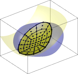
(d) Surface FEM

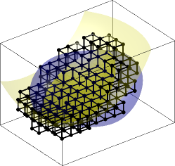
(e) Trace FEM

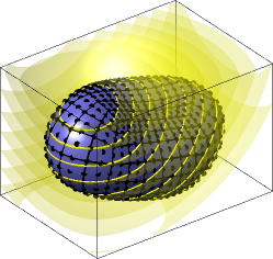
(f) Bulk Trace FEM

Figure 9: Variants of the FEM for BVPs on curved lines ((a) to (c)) and surfaces ((d) to (f)) with focus on the employed meshes; note that the number and order of the elements is only examplarily. The classical Surface FEM applies to (a) and (d) where the manifold is discretized by a conforming mesh, (b) and (e) is the Trace FEM where the zero-level set is the domain of interest and the cut elements of a background mesh are used for the discretization, (c) and (f) is the proposed Bulk Trace FEM where the bulk domain is discretized and BVPs on all level sets are considered simultaneously.

For the simultaneous analysis of structures implied by all level sets over a bulk domain as proposed herein, the bulk domain $\Omega_{\mathchoice{\displaystyle\boldsymbol{X}}{\textstyle\boldsymbol{X}}{\scriptstyle\boldsymbol{X}}{\scriptscriptstyle\boldsymbol{X}}}$ is discretized by a background mesh which is conforming to the boundary $\partial\Omega_{\mathchoice{\displaystyle\boldsymbol{X}}{\textstyle\boldsymbol{X}}{\scriptstyle\boldsymbol{X}}{\scriptscriptstyle\boldsymbol{X}}}$ (and, hence, also $\partial\Gamma_{\!\!\mathchoice{\displaystyle\boldsymbol{X}}{\textstyle\boldsymbol{X}}{\scriptstyle\boldsymbol{X}}{\scriptscriptstyle\boldsymbol{X}}}^{c}$), yet typically not conforming to the individual level sets $\Gamma_{\!\!\mathchoice{\displaystyle\boldsymbol{X}}{\textstyle\boldsymbol{X}}{\scriptstyle\boldsymbol{X}}{\scriptscriptstyle\boldsymbol{X}}}^{c}$ of $\phi$, see Figs. 9(c) and (f). The method is similar to the Trace FEM in that it uses test and trial functions for the numerical analysis which are implied by the $d$-dimensional background mesh. However, no special numerical integration and stabilization is needed (as there are no cut elements), and boundary conditions are enforced as in the Surface FEM. Therefore, the numerical method employed here, and closely related to [29, 27, 26, 6] for transport problems, may be seen as a hybrid between the Surface and Trace FEM. Hence, we label this approach the Bulk Trace FEM.

It is noted that formulating the mechanical models for ropes and membranes based on the tangential differential calculus using surface operators as in the previous section results in a unified and general description which may be used in all the resulting variants of the FEM with only minor adaptions. This was already emphasized in [58, 59, 36] in the context of the Surface and Trace FEM and is herein confirmed for the proposed Bulk Trace FEM.

4.1 Governing equations in weak form

For any FEM simulations, it is necessary to state the governing equations in weak form. Therefore, the following test and trial function spaces are introduced,

$$\mathcal{S}_{\mathchoice{\displaystyle\boldsymbol{u}}{\textstyle\boldsymbol{u}}{\scriptstyle\boldsymbol{u}}{\scriptscriptstyle\boldsymbol{u}}} =\left\{\mathchoice{\displaystyle\boldsymbol{v}}{\textstyle\boldsymbol{v}}{\scriptstyle\boldsymbol{v}}{\scriptscriptstyle\boldsymbol{v}}\in\left[\mathcal{H}^{1}(\Omega_{\mathchoice{\displaystyle\boldsymbol{X}}{\textstyle\boldsymbol{X}}{\scriptstyle\boldsymbol{X}}{\scriptscriptstyle\boldsymbol{X}}})\right]^{d}:\ \mathchoice{\displaystyle\boldsymbol{v}}{\textstyle\boldsymbol{v}}{\scriptstyle\boldsymbol{v}}{\scriptscriptstyle\boldsymbol{v}}=\hat{\mathchoice{\displaystyle\boldsymbol{G}}{\textstyle\boldsymbol{G}}{\scriptstyle\boldsymbol{G}}{\scriptscriptstyle\boldsymbol{G}}}\ \text{on}\ \partial\Omega_{\mathchoice{\displaystyle\boldsymbol{X}}{\textstyle\boldsymbol{X}}{\scriptstyle\boldsymbol{X}}{\scriptscriptstyle\boldsymbol{X}},\mathrm{D}}\right\},$$ (4.1)

$$\mathcal{V}_{\mathchoice{\displaystyle\boldsymbol{u}}{\textstyle\boldsymbol{u}}{\scriptstyle\boldsymbol{u}}{\scriptscriptstyle\boldsymbol{u}}} =\left\{\mathchoice{\displaystyle\boldsymbol{v}}{\textstyle\boldsymbol{v}}{\scriptstyle\boldsymbol{v}}{\scriptscriptstyle\boldsymbol{v}}\in\left[\mathcal{H}^{1}(\Omega_{\mathchoice{\displaystyle\boldsymbol{X}}{\textstyle\boldsymbol{X}}{\scriptstyle\boldsymbol{X}}{\scriptscriptstyle\boldsymbol{X}}})\right]^{d}:\ \mathchoice{\displaystyle\boldsymbol{v}}{\textstyle\boldsymbol{v}}{\scriptstyle\boldsymbol{v}}{\scriptscriptstyle\boldsymbol{v}}=\mathchoice{\displaystyle\boldsymbol{0}}{\textstyle\boldsymbol{0}}{\scriptstyle\boldsymbol{0}}{\scriptscriptstyle\boldsymbol{0}}\ \text{on}\ \partial\Omega_{\mathchoice{\displaystyle\boldsymbol{X}}{\textstyle\boldsymbol{X}}{\scriptstyle\boldsymbol{X}}{\scriptscriptstyle\boldsymbol{X}},\mathrm{D}}\right\},$$ (4.2)

where $\mathcal{H}^{1}$ is the Sobolev space of functions with square integrable first derivatives. The task is to find $\mathchoice{\displaystyle\boldsymbol{u}}{\textstyle\boldsymbol{u}}{\scriptstyle\boldsymbol{u}}{\scriptscriptstyle\boldsymbol{u}}\in\mathcal{S}_{\mathchoice{\displaystyle\boldsymbol{u}}{\textstyle\boldsymbol{u}}{\scriptstyle\boldsymbol{u}}{\scriptscriptstyle\boldsymbol{u}}}$ such that for all $\mathchoice{\displaystyle\boldsymbol{w}}{\textstyle\boldsymbol{w}}{\scriptstyle\boldsymbol{w}}{\scriptscriptstyle\boldsymbol{w}}\in\mathcal{V}_{\mathchoice{\displaystyle\boldsymbol{u}}{\textstyle\boldsymbol{u}}{\scriptstyle\boldsymbol{u}}{\scriptscriptstyle\boldsymbol{u}}}$, there holds

$$\int_{\Omega_{\mathchoice{\displaystyle\boldsymbol{X}}{\textstyle\boldsymbol{X}}{\scriptstyle\boldsymbol{X}}{\scriptscriptstyle\boldsymbol{X}}}}\nabla_{\mathchoice{\displaystyle\boldsymbol{X}}{\textstyle\boldsymbol{X}}{\scriptstyle\boldsymbol{X}}{\scriptscriptstyle\boldsymbol{X}}}^{\Gamma,\mathrm{dir}}\mathchoice{\displaystyle\boldsymbol{w}}{\textstyle\boldsymbol{w}}{\scriptstyle\boldsymbol{w}}{\scriptscriptstyle\boldsymbol{w}}:\mathchoice{\displaystyle\mathbf{K}}{\textstyle\mathbf{K}}{\scriptstyle\mathbf{K}}{\scriptscriptstyle\mathbf{K}}\left(\mathchoice{\displaystyle\boldsymbol{u}}{\textstyle\boldsymbol{u}}{\scriptstyle\boldsymbol{u}}{\scriptscriptstyle\boldsymbol{u}}\right)\cdot\left\|\nabla_{\!\!\mathchoice{\displaystyle\boldsymbol{X}}{\textstyle\boldsymbol{X}}{\scriptstyle\boldsymbol{X}}{\scriptscriptstyle\boldsymbol{X}}}\phi\right\|\,\mathrm{d}\Omega =\int_{\Omega_{\mathchoice{\displaystyle\boldsymbol{X}}{\textstyle\boldsymbol{X}}{\scriptstyle\boldsymbol{X}}{\scriptscriptstyle\boldsymbol{X}}}}\!\!\!\mathchoice{\displaystyle\boldsymbol{w}}{\textstyle\boldsymbol{w}}{\scriptstyle\boldsymbol{w}}{\scriptscriptstyle\boldsymbol{w}}\cdot\mathchoice{\displaystyle\boldsymbol{F}}{\textstyle\boldsymbol{F}}{\scriptstyle\boldsymbol{F}}{\scriptscriptstyle\boldsymbol{F}}\cdot\left\|\nabla_{\!\!\mathchoice{\displaystyle\boldsymbol{X}}{\textstyle\boldsymbol{X}}{\scriptstyle\boldsymbol{X}}{\scriptscriptstyle\boldsymbol{X}}}\phi\right\|\,\mathrm{d}\Omega$$ (4.3)

$$+\int_{\partial\Omega_{\mathchoice{\displaystyle\boldsymbol{X}}{\textstyle\boldsymbol{X}}{\scriptstyle\boldsymbol{X}}{\scriptscriptstyle\boldsymbol{X}},\text{N}}}\!\!\!\!\!\!\mathchoice{\displaystyle\boldsymbol{w}}{\textstyle\boldsymbol{w}}{\scriptstyle\boldsymbol{w}}{\scriptscriptstyle\boldsymbol{w}}\cdot\hat{\mathchoice{\displaystyle\boldsymbol{H}}{\textstyle\boldsymbol{H}}{\scriptstyle\boldsymbol{H}}{\scriptscriptstyle\boldsymbol{H}}}\cdot\left(\mathchoice{\displaystyle\boldsymbol{Q}}{\textstyle\boldsymbol{Q}}{\scriptstyle\boldsymbol{Q}}{\scriptscriptstyle\boldsymbol{Q}}\cdot\mathchoice{\displaystyle\boldsymbol{M}}{\textstyle\boldsymbol{M}}{\scriptstyle\boldsymbol{M}}{\scriptscriptstyle\boldsymbol{M}}\right)\cdot\left\|\nabla_{\!\!\mathchoice{\displaystyle\boldsymbol{X}}{\textstyle\boldsymbol{X}}{\scriptstyle\boldsymbol{X}}{\scriptscriptstyle\boldsymbol{X}}}\phi\right\|\;\mathrm{d}\partial\Omega$$ (4.4)

This weak form is obtained after the following sequence of steps: Multiply Eq. (3.14) with test functions $\mathchoice{\displaystyle\boldsymbol{w}}{\textstyle\boldsymbol{w}}{\scriptstyle\boldsymbol{w}}{\scriptscriptstyle\boldsymbol{w}}$$\left(\mathchoice{\displaystyle\boldsymbol{X}}{\textstyle\boldsymbol{X}}{\scriptstyle\boldsymbol{X}}{\scriptscriptstyle\boldsymbol{X}}\right)$ and integrate over the level sets in some interval $\int_{\phi^{\min}}^{\phi^{\max}}\int_{\Gamma_{\!\!\mathchoice{\displaystyle\boldsymbol{X}}{\textstyle\boldsymbol{X}}{\scriptstyle\boldsymbol{X}}{\scriptscriptstyle\boldsymbol{X}}}^{c}}\square\,\mathrm{d\Gamma}\,\mathrm{d}c$ which, through the co-area formula (2.26) is converted into an integral over the bulk domain $\int_{\Omega_{\mathchoice{\displaystyle\boldsymbol{X}}{\textstyle\boldsymbol{X}}{\scriptstyle\boldsymbol{X}}{\scriptscriptstyle\boldsymbol{X}}}}\square\cdot\left\|\nabla_{\!\!\mathchoice{\displaystyle\boldsymbol{X}}{\textstyle\boldsymbol{X}}{\scriptstyle\boldsymbol{X}}{\scriptscriptstyle\boldsymbol{X}}}\phi\right\|\,\mathrm{d\Omega}$. Then, the divergence theorem for tensors (2.31) is applied to obtain (4.3), noting that the curvature term vanishes due to $\mathchoice{\displaystyle\mathbf{K}}{\textstyle\mathbf{K}}{\scriptstyle\mathbf{K}}{\scriptscriptstyle\mathbf{K}}\cdot\mathchoice{\displaystyle\boldsymbol{N}}{\textstyle\boldsymbol{N}}{\scriptstyle\boldsymbol{N}}{\scriptscriptstyle\boldsymbol{N}}=\mathchoice{\displaystyle\boldsymbol{0}}{\textstyle\boldsymbol{0}}{\scriptstyle\boldsymbol{0}}{\scriptscriptstyle\boldsymbol{0}}$. A similar weak form could be posed over the deformed configuration which, however, would be less desirable for the numerical analysis (as it would require mesh updates during the iterative procedure to solve this non-linear problem).

4.2 Discretized weak form

Let there be a discretization of the bulk domain, $\Omega_{\mathchoice{\displaystyle\boldsymbol{X}}{\textstyle\boldsymbol{X}}{\scriptstyle\boldsymbol{X}}{\scriptscriptstyle\boldsymbol{X}}}^{h}$, in the form of a conforming, $d$-dimensional mesh, herein composed by higher-order elements of the Lagrange type with equally spaced nodes in the reference element (with arbitrary element types such as triangular/quadrilateral in 2D, or tetrahedral/hexahedral in 3D). The nodal coordinates in the undeformed configuration are labeled $\mathchoice{\displaystyle\boldsymbol{X}}{\textstyle\boldsymbol{X}}{\scriptstyle\boldsymbol{X}}{\scriptscriptstyle\boldsymbol{X}}_{i}$ with $i=1,\dots,n_{q}$ and $n_{q}$ being the number of nodes in the mesh, see Figs. 9(c) and (f) for generic examples. The resulting nodal basis functions $B_{i}\!\left(\mathchoice{\displaystyle\boldsymbol{X}}{\textstyle\boldsymbol{X}}{\scriptstyle\boldsymbol{X}}{\scriptscriptstyle\boldsymbol{X}}\right)$, used as test and trial functions, span a $C^{0}$-continuous finite element space as

$$\mathcal{Q}_{\Omega_{\mathchoice{\displaystyle\boldsymbol{X}}{\textstyle\boldsymbol{X}}{\scriptstyle\boldsymbol{X}}{\scriptscriptstyle\boldsymbol{X}}}}^{h}:=\left\{v_{h}\in C^{0}(\Omega_{\mathchoice{\displaystyle\boldsymbol{X}}{\textstyle\boldsymbol{X}}{\scriptstyle\boldsymbol{X}}{\scriptscriptstyle\boldsymbol{X}}}^{h}):\ v_{h}=\sum_{i=1}^{n_{q}}B_{i}(\mathchoice{\displaystyle\boldsymbol{X}}{\textstyle\boldsymbol{X}}{\scriptstyle\boldsymbol{X}}{\scriptscriptstyle\boldsymbol{X}})\cdot\hat{v}_{i}\text{ with }\hat{v}_{i}\in\mathbb{R}\right\}\subset\mathcal{H}^{1}(\Omega_{\mathchoice{\displaystyle\boldsymbol{X}}{\textstyle\boldsymbol{X}}{\scriptstyle\boldsymbol{X}}{\scriptscriptstyle\boldsymbol{X}}}^{h})\ .$$ (4.5)

$B_{i}(\mathchoice{\displaystyle\boldsymbol{X}}{\textstyle\boldsymbol{X}}{\scriptstyle\boldsymbol{X}}{\scriptscriptstyle\boldsymbol{X}})$ are obtained from isoparametric mappings from the $d$-dimensional reference element to the physical elements. Furthermore, the level-set function $\phi$ is replaced by its interpolation $\phi_{h}\left(\mathchoice{\displaystyle\boldsymbol{X}}{\textstyle\boldsymbol{X}}{\scriptstyle\boldsymbol{X}}{\scriptscriptstyle\boldsymbol{X}}\right)\in\mathcal{Q}_{\Omega_{\mathchoice{\displaystyle\boldsymbol{X}}{\textstyle\boldsymbol{X}}{\scriptstyle\boldsymbol{X}}{\scriptscriptstyle\boldsymbol{X}}}}^{h}$ with prescribed nodal values $\hat{\phi}_{i}=\phi\left(\mathchoice{\displaystyle\boldsymbol{X}}{\textstyle\boldsymbol{X}}{\scriptstyle\boldsymbol{X}}{\scriptscriptstyle\boldsymbol{X}}_{i}\right)$. Based on Eq. (4.5), the following discrete test and trial function spaces are introduced

$$\mathcal{S}_{\Omega_{\mathchoice{\displaystyle\boldsymbol{X}}{\textstyle\boldsymbol{X}}{\scriptstyle\boldsymbol{X}}{\scriptscriptstyle\boldsymbol{X}}}}^{h} =\left\{\mathchoice{\displaystyle\boldsymbol{v}}{\textstyle\boldsymbol{v}}{\scriptstyle\boldsymbol{v}}{\scriptscriptstyle\boldsymbol{v}}_{h}\in\left[\mathcal{Q}_{\Omega_{\mathchoice{\displaystyle\boldsymbol{X}}{\textstyle\boldsymbol{X}}{\scriptstyle\boldsymbol{X}}{\scriptscriptstyle\boldsymbol{X}}}}^{h}\right]^{d}:\ \mathchoice{\displaystyle\boldsymbol{v}}{\textstyle\boldsymbol{v}}{\scriptstyle\boldsymbol{v}}{\scriptscriptstyle\boldsymbol{v}}_{h}=\hat{\mathchoice{\displaystyle\boldsymbol{G}}{\textstyle\boldsymbol{G}}{\scriptstyle\boldsymbol{G}}{\scriptscriptstyle\boldsymbol{G}}}\ \text{on}\ \partial\Omega_{\mathchoice{\displaystyle\boldsymbol{X}}{\textstyle\boldsymbol{X}}{\scriptstyle\boldsymbol{X}}{\scriptscriptstyle\boldsymbol{X}},\mathrm{D}}^{h}\right\},$$ (4.6)

$$\mathcal{V}_{\Omega_{\mathchoice{\displaystyle\boldsymbol{X}}{\textstyle\boldsymbol{X}}{\scriptstyle\boldsymbol{X}}{\scriptscriptstyle\boldsymbol{X}}}}^{h} =\left\{\mathchoice{\displaystyle\boldsymbol{v}}{\textstyle\boldsymbol{v}}{\scriptstyle\boldsymbol{v}}{\scriptscriptstyle\boldsymbol{v}}_{h}\in\left[\mathcal{Q}_{\Omega_{\mathchoice{\displaystyle\boldsymbol{X}}{\textstyle\boldsymbol{X}}{\scriptstyle\boldsymbol{X}}{\scriptscriptstyle\boldsymbol{X}}}}^{h}\right]^{d}:\ \mathchoice{\displaystyle\boldsymbol{v}}{\textstyle\boldsymbol{v}}{\scriptstyle\boldsymbol{v}}{\scriptscriptstyle\boldsymbol{v}}_{h}=\mathchoice{\displaystyle\boldsymbol{0}}{\textstyle\boldsymbol{0}}{\scriptstyle\boldsymbol{0}}{\scriptscriptstyle\boldsymbol{0}}\ \text{on}\ \partial\Omega_{\mathchoice{\displaystyle\boldsymbol{X}}{\textstyle\boldsymbol{X}}{\scriptstyle\boldsymbol{X}}{\scriptscriptstyle\boldsymbol{X}},\mathrm{D}}^{h}\right\}.$$ (4.7)

The discrete weak form of Eq. (4.3) reads as follows: Given the level-set function $\phi_{h}$, Lamé constants $(\lambda,\mu)\in\mathbb{R}^{+}$, body forces $\mathchoice{\displaystyle\boldsymbol{F}}{\textstyle\boldsymbol{F}}{\scriptstyle\boldsymbol{F}}{\scriptscriptstyle\boldsymbol{F}}\in\mathbb{R}^{d}$ on $\Omega_{\mathchoice{\displaystyle\boldsymbol{X}}{\textstyle\boldsymbol{X}}{\scriptstyle\boldsymbol{X}}{\scriptscriptstyle\boldsymbol{X}}}^{h}$, tractions $\hat{\mathchoice{\displaystyle\boldsymbol{H}}{\textstyle\boldsymbol{H}}{\scriptstyle\boldsymbol{H}}{\scriptscriptstyle\boldsymbol{H}}}\in\mathbb{R}^{d}$ on $\partial\Omega_{\mathchoice{\displaystyle\boldsymbol{X}}{\textstyle\boldsymbol{X}}{\scriptstyle\boldsymbol{X}}{\scriptscriptstyle\boldsymbol{X}},\text{N}}^{h}$, find the displacement field $\mathchoice{\displaystyle\boldsymbol{u}}{\textstyle\boldsymbol{u}}{\scriptstyle\boldsymbol{u}}{\scriptscriptstyle\boldsymbol{u}}_{h}\in\mathcal{S}_{\Omega_{\mathchoice{\displaystyle\boldsymbol{X}}{\textstyle\boldsymbol{X}}{\scriptstyle\boldsymbol{X}}{\scriptscriptstyle\boldsymbol{X}}}}^{h}$ such that for all test functions $\mathchoice{\displaystyle\boldsymbol{w}}{\textstyle\boldsymbol{w}}{\scriptstyle\boldsymbol{w}}{\scriptscriptstyle\boldsymbol{w}}_{h}\in\mathcal{V}_{\Omega_{\mathchoice{\displaystyle\boldsymbol{X}}{\textstyle\boldsymbol{X}}{\scriptstyle\boldsymbol{X}}{\scriptscriptstyle\boldsymbol{X}}}}^{h}$ there holds in $\Omega_{\mathchoice{\displaystyle\boldsymbol{X}}{\textstyle\boldsymbol{X}}{\scriptstyle\boldsymbol{X}}{\scriptscriptstyle\boldsymbol{X}}}^{h}$:

$$\int_{\Omega_{\mathchoice{\displaystyle\boldsymbol{X}}{\textstyle\boldsymbol{X}}{\scriptstyle\boldsymbol{X}}{\scriptscriptstyle\boldsymbol{X}}}^{h}}\nabla_{\mathchoice{\displaystyle\boldsymbol{X}}{\textstyle\boldsymbol{X}}{\scriptstyle\boldsymbol{X}}{\scriptscriptstyle\boldsymbol{X}}}^{\Gamma,\mathrm{dir}}\mathchoice{\displaystyle\boldsymbol{w}}{\textstyle\boldsymbol{w}}{\scriptstyle\boldsymbol{w}}{\scriptscriptstyle\boldsymbol{w}}_{h}:\mathchoice{\displaystyle\mathbf{K}}{\textstyle\mathbf{K}}{\scriptstyle\mathbf{K}}{\scriptscriptstyle\mathbf{K}}\left(\mathchoice{\displaystyle\boldsymbol{u}}{\textstyle\boldsymbol{u}}{\scriptstyle\boldsymbol{u}}{\scriptscriptstyle\boldsymbol{u}}_{h}\right)\cdot\left\|\nabla_{\!\!\mathchoice{\displaystyle\boldsymbol{X}}{\textstyle\boldsymbol{X}}{\scriptstyle\boldsymbol{X}}{\scriptscriptstyle\boldsymbol{X}}}\phi_{h}\right\|\,\mathrm{d}\Omega= \int_{\Omega_{\mathchoice{\displaystyle\boldsymbol{X}}{\textstyle\boldsymbol{X}}{\scriptstyle\boldsymbol{X}}{\scriptscriptstyle\boldsymbol{X}}}^{h}}\!\!\!\mathchoice{\displaystyle\boldsymbol{w}}{\textstyle\boldsymbol{w}}{\scriptstyle\boldsymbol{w}}{\scriptscriptstyle\boldsymbol{w}}_{h}\cdot\mathchoice{\displaystyle\boldsymbol{F}}{\textstyle\boldsymbol{F}}{\scriptstyle\boldsymbol{F}}{\scriptscriptstyle\boldsymbol{F}}\cdot\left\|\nabla_{\!\!\mathchoice{\displaystyle\boldsymbol{X}}{\textstyle\boldsymbol{X}}{\scriptstyle\boldsymbol{X}}{\scriptscriptstyle\boldsymbol{X}}}\phi_{h}\right\|\,\mathrm{d}\Omega$$ (4.8)

$$+\int_{\partial\Omega_{\mathchoice{\displaystyle\boldsymbol{X}}{\textstyle\boldsymbol{X}}{\scriptstyle\boldsymbol{X}}{\scriptscriptstyle\boldsymbol{X}},\text{N}}^{h}}\!\!\!\!\!\!\mathchoice{\displaystyle\boldsymbol{w}}{\textstyle\boldsymbol{w}}{\scriptstyle\boldsymbol{w}}{\scriptscriptstyle\boldsymbol{w}}_{h}\cdot\hat{\mathchoice{\displaystyle\boldsymbol{H}}{\textstyle\boldsymbol{H}}{\scriptstyle\boldsymbol{H}}{\scriptscriptstyle\boldsymbol{H}}}\cdot\left(\mathchoice{\displaystyle\boldsymbol{Q}}{\textstyle\boldsymbol{Q}}{\scriptstyle\boldsymbol{Q}}{\scriptscriptstyle\boldsymbol{Q}}_{h}\cdot\mathchoice{\displaystyle\boldsymbol{M}}{\textstyle\boldsymbol{M}}{\scriptstyle\boldsymbol{M}}{\scriptscriptstyle\boldsymbol{M}}_{h}\right)\cdot\left\|\nabla_{\!\!\mathchoice{\displaystyle\boldsymbol{X}}{\textstyle\boldsymbol{X}}{\scriptstyle\boldsymbol{X}}{\scriptscriptstyle\boldsymbol{X}}}\phi_{h}\right\|\;\mathrm{d}\partial\Omega.$$ (4.9)

For brevity, we avoid adding an $h$ also to the discretized differential operators, e.g., we do not write $\nabla_{\!\!\mathchoice{\displaystyle\boldsymbol{X}}{\textstyle\boldsymbol{X}}{\scriptstyle\boldsymbol{X}}{\scriptscriptstyle\boldsymbol{X}}}^{h}$. The sought discrete displacement field $\mathchoice{\displaystyle\boldsymbol{u}}{\textstyle\boldsymbol{u}}{\scriptstyle\boldsymbol{u}}{\scriptscriptstyle\boldsymbol{u}}_{h}(\mathchoice{\displaystyle\boldsymbol{X}}{\textstyle\boldsymbol{X}}{\scriptstyle\boldsymbol{X}}{\scriptscriptstyle\boldsymbol{X}})$ is obtained solving a non-linear system of equations for the $n_{\text{DOF}}=d\cdot n_{q}$ nodal values (degrees of freedom) as usual in the context of finite strain theory.

4.3 Technical aspects

For the implementation of the Bulk Trace FEM, some useful hints are given next. It is found beneficial to split the implementation into an application-independent part related to finite element technology and the part which is related to the concrete BVP of interest, i.e., the application. The first part may be reused in any other Bulk Trace FEM simulation, e.g., in the context of solving transport problems on all level sets in a bulk domain. Of course, the situation in the reference elements is completely identical to any other FE application and not further detailed here. As such, a standard set of integration points and element functions, being related to the type and order of the reference element, is given as a starting point. Let the reference element feature the nodal coordinates $\mathchoice{\displaystyle\boldsymbol{r}}{\textstyle\boldsymbol{r}}{\scriptstyle\boldsymbol{r}}{\scriptscriptstyle\boldsymbol{r}}_{i}$ and element functions $B_{i}\left(\mathchoice{\displaystyle\boldsymbol{r}}{\textstyle\boldsymbol{r}}{\scriptstyle\boldsymbol{r}}{\scriptscriptstyle\boldsymbol{r}}\right)$ with $i=1,\dots n^{\mathrm{npe}}$ and $n^{\mathrm{npe}}$ being the number of nodes per element. A proper Gauss quadrature rule, related to the order of the reference element, is defined by a set of $n^{\mathrm{int}}$ integration points $\mathchoice{\displaystyle\boldsymbol{r}}{\textstyle\boldsymbol{r}}{\scriptstyle\boldsymbol{r}}{\scriptscriptstyle\boldsymbol{r}}_{i}^{\mathrm{int}}$ and weights $w_{i}^{\mathrm{int,ref}}$ with $i=1,\dots n^{\mathrm{int}}$.

The mapping from the reference element to any of the physical elements in the undeformed configuration is given by the isoparametric concept, $\mathchoice{\displaystyle\boldsymbol{X}}{\textstyle\boldsymbol{X}}{\scriptstyle\boldsymbol{X}}{\scriptscriptstyle\boldsymbol{X}}\!\left(\mathchoice{\displaystyle\boldsymbol{r}}{\textstyle\boldsymbol{r}}{\scriptstyle\boldsymbol{r}}{\scriptscriptstyle\boldsymbol{r}}\right)=\sum_{i=1}^{n^{\mathrm{npe}}}B_{i}\!\left(\mathchoice{\displaystyle\boldsymbol{r}}{\textstyle\boldsymbol{r}}{\scriptstyle\boldsymbol{r}}{\scriptscriptstyle\boldsymbol{r}}\right)\cdot\mathchoice{\displaystyle\boldsymbol{X}}{\textstyle\boldsymbol{X}}{\scriptstyle\boldsymbol{X}}{\scriptscriptstyle\boldsymbol{X}}_{i}^{\mathrm{el}}$ where $\mathchoice{\displaystyle\boldsymbol{X}}{\textstyle\boldsymbol{X}}{\scriptstyle\boldsymbol{X}}{\scriptscriptstyle\boldsymbol{X}}_{i}^{\mathrm{el}}$ are the respective nodal element coordinates. In every element, this results in mapped integration points $\mathchoice{\displaystyle\boldsymbol{X}}{\textstyle\boldsymbol{X}}{\scriptstyle\boldsymbol{X}}{\scriptscriptstyle\boldsymbol{X}}_{i}^{\mathrm{int}}$ with modified integration weights $w_{i}^{\mathrm{int,phys}}$. In a standard FE context, $w_{i}^{\mathrm{int,phys}}=w_{i}^{\mathrm{int,ref}}\cdot\det\mathchoice{\displaystyle\mathbf{J}}{\textstyle\mathbf{J}}{\scriptstyle\mathbf{J}}{\scriptscriptstyle\mathbf{J}}\left(\mathchoice{\displaystyle\boldsymbol{r}}{\textstyle\boldsymbol{r}}{\scriptstyle\boldsymbol{r}}{\scriptscriptstyle\boldsymbol{r}}_{i}^{\mathrm{int}}\right)$ where $\mathchoice{\displaystyle\mathbf{J}}{\textstyle\mathbf{J}}{\scriptstyle\mathbf{J}}{\scriptscriptstyle\mathbf{J}}=\nicefrac{{\partial\mathchoice{\displaystyle\boldsymbol{X}}{\textstyle\boldsymbol{X}}{\scriptstyle\boldsymbol{X}}{\scriptscriptstyle\boldsymbol{X}}}}{{\partial\mathchoice{\displaystyle\boldsymbol{r}}{\textstyle\boldsymbol{r}}{\scriptstyle\boldsymbol{r}}{\scriptscriptstyle\boldsymbol{r}}}}$ is the Jacobi matrix of the finite element map. However, because all domain integrals in Eq. (4.8) involve the term $\left\|\nabla_{\!\!\mathchoice{\displaystyle\boldsymbol{X}}{\textstyle\boldsymbol{X}}{\scriptstyle\boldsymbol{X}}{\scriptscriptstyle\boldsymbol{X}}}\phi_{h}\right\|$, it is useful to also modify the weights according to this term as well, hence,

$$\int_{\Omega_{\mathchoice{\displaystyle\boldsymbol{X}}{\textstyle\boldsymbol{X}}{\scriptstyle\boldsymbol{X}}{\scriptscriptstyle\boldsymbol{X}}}^{\mathrm{el}}}f\left(\mathchoice{\displaystyle\boldsymbol{X}}{\textstyle\boldsymbol{X}}{\scriptstyle\boldsymbol{X}}{\scriptscriptstyle\boldsymbol{X}}\right)\cdot\left\|\nabla_{\!\!\mathchoice{\displaystyle\boldsymbol{X}}{\textstyle\boldsymbol{X}}{\scriptstyle\boldsymbol{X}}{\scriptscriptstyle\boldsymbol{X}}}\phi_{h}\left(\mathchoice{\displaystyle\boldsymbol{X}}{\textstyle\boldsymbol{X}}{\scriptstyle\boldsymbol{X}}{\scriptscriptstyle\boldsymbol{X}}\right)\right\|\,\mathrm{d}\Omega\approx \;\sum_{i=1}^{n^{\mathrm{int}}}f\left(\mathchoice{\displaystyle\boldsymbol{X}}{\textstyle\boldsymbol{X}}{\scriptstyle\boldsymbol{X}}{\scriptscriptstyle\boldsymbol{X}}_{i}^{\mathrm{int}}\right)\cdot w_{i}^{\mathrm{int,phys}},$$

$$\text{with }w_{i}^{\mathrm{int,phys}}= \;w_{i}^{\mathrm{int,ref}}\cdot\left\|\nabla_{\!\!\mathchoice{\displaystyle\boldsymbol{X}}{\textstyle\boldsymbol{X}}{\scriptstyle\boldsymbol{X}}{\scriptscriptstyle\boldsymbol{X}}}\phi_{h}\left(\mathchoice{\displaystyle\boldsymbol{X}}{\textstyle\boldsymbol{X}}{\scriptstyle\boldsymbol{X}}{\scriptscriptstyle\boldsymbol{X}}_{i}^{\mathrm{int}}\right)\right\|\cdot\det\left(\mathchoice{\displaystyle\mathbf{J}}{\textstyle\mathbf{J}}{\scriptstyle\mathbf{J}}{\scriptscriptstyle\mathbf{J}}\left(\mathchoice{\displaystyle\boldsymbol{r}}{\textstyle\boldsymbol{r}}{\scriptstyle\boldsymbol{r}}{\scriptscriptstyle\boldsymbol{r}}_{i}^{\mathrm{int}}\right)\right),$$

$$\text{and $\nabla_{\!\!\mathchoice{\displaystyle\boldsymbol{X}}{\textstyle\boldsymbol{X}}{\scriptstyle\boldsymbol{X}}{\scriptscriptstyle\boldsymbol{X}}}\phi_{h}\left(\mathchoice{\displaystyle\boldsymbol{X}}{\textstyle\boldsymbol{X}}{\scriptstyle\boldsymbol{X}}{\scriptscriptstyle\boldsymbol{X}}(\mathchoice{\displaystyle\boldsymbol{r}}{\textstyle\boldsymbol{r}}{\scriptstyle\boldsymbol{r}}{\scriptscriptstyle\boldsymbol{r}}_{i}^{\mathrm{int}})\right)$}= \;\mathchoice{\displaystyle\mathbf{J}}{\textstyle\mathbf{J}}{\scriptstyle\mathbf{J}}{\scriptscriptstyle\mathbf{J}}^{-\mathrm{T}}\!\left(\mathchoice{\displaystyle\boldsymbol{r}}{\textstyle\boldsymbol{r}}{\scriptstyle\boldsymbol{r}}{\scriptscriptstyle\boldsymbol{r}}_{i}^{\mathrm{int}}\right)\cdot\nabla_{\!\mathchoice{\displaystyle\boldsymbol{r}}{\textstyle\boldsymbol{r}}{\scriptstyle\boldsymbol{r}}{\scriptscriptstyle\boldsymbol{r}}}\phi_{h}\left(\mathchoice{\displaystyle\boldsymbol{r}}{\textstyle\boldsymbol{r}}{\scriptstyle\boldsymbol{r}}{\scriptscriptstyle\boldsymbol{r}}_{i}^{\mathrm{int}}\right).$$

It is also found useful to apply some standard differential operators such as the gradient operator to the test and trial functions in the FE analysis which may also be recycled in various applications of the Bulk Trace FEM. For example, when the gradients $\nabla_{\!\mathchoice{\displaystyle\boldsymbol{X}}{\textstyle\boldsymbol{X}}{\scriptstyle\boldsymbol{X}}{\scriptscriptstyle\boldsymbol{X}}}B_{i}$ are precomputed, it is trivial to specify the gradient of some (scalar) approximation as $\nabla_{\!\mathchoice{\displaystyle\boldsymbol{X}}{\textstyle\boldsymbol{X}}{\scriptstyle\boldsymbol{X}}{\scriptscriptstyle\boldsymbol{X}}}u_{h}=\sum_{i}\nabla_{\!\mathchoice{\displaystyle\boldsymbol{X}}{\textstyle\boldsymbol{X}}{\scriptstyle\boldsymbol{X}}{\scriptscriptstyle\boldsymbol{X}}}B_{i}\cdot\hat{u}_{i}$. Of course, in the reference element, differential operators with respect to the coordinates $\mathchoice{\displaystyle\boldsymbol{r}}{\textstyle\boldsymbol{r}}{\scriptstyle\boldsymbol{r}}{\scriptscriptstyle\boldsymbol{r}}$ may easily be applied to the element functions, e.g., to generate $\nabla_{\mathchoice{\displaystyle\boldsymbol{r}}{\textstyle\boldsymbol{r}}{\scriptstyle\boldsymbol{r}}{\scriptscriptstyle\boldsymbol{r}}}B_{i}\left(\mathchoice{\displaystyle\boldsymbol{r}}{\textstyle\boldsymbol{r}}{\scriptstyle\boldsymbol{r}}{\scriptscriptstyle\boldsymbol{r}}\right)$. Upon mapping these functions to the (undeformed) physical elements and seeking the standard (bulk) gradient with respect to the coordinates $\mathchoice{\displaystyle\boldsymbol{X}}{\textstyle\boldsymbol{X}}{\scriptstyle\boldsymbol{X}}{\scriptscriptstyle\boldsymbol{X}}$, we have $\nabla_{\mathchoice{\displaystyle\boldsymbol{X}}{\textstyle\boldsymbol{X}}{\scriptstyle\boldsymbol{X}}{\scriptscriptstyle\boldsymbol{X}}}B_{i}\left(\mathchoice{\displaystyle\boldsymbol{X}}{\textstyle\boldsymbol{X}}{\scriptstyle\boldsymbol{X}}{\scriptscriptstyle\boldsymbol{X}}\right)=\mathchoice{\displaystyle\mathbf{J}}{\textstyle\mathbf{J}}{\scriptstyle\mathbf{J}}{\scriptscriptstyle\mathbf{J}}^{-\mathrm{T}}\left(\mathchoice{\displaystyle\boldsymbol{r}}{\textstyle\boldsymbol{r}}{\scriptstyle\boldsymbol{r}}{\scriptscriptstyle\boldsymbol{r}}\right)\cdot\nabla_{\mathchoice{\displaystyle\boldsymbol{r}}{\textstyle\boldsymbol{r}}{\scriptstyle\boldsymbol{r}}{\scriptscriptstyle\boldsymbol{r}}}B_{i}\left(\mathchoice{\displaystyle\boldsymbol{r}}{\textstyle\boldsymbol{r}}{\scriptstyle\boldsymbol{r}}{\scriptscriptstyle\boldsymbol{r}}\right)$ as usual. As discussed in Section 2, in the Bulk Trace FEM, differential operators with respect to the level sets of $\phi$ play a crucial role. For the surface gradient of the element functions $B_{i}$, we have

$$\nabla_{\!\mathchoice{\displaystyle\boldsymbol{X}}{\textstyle\boldsymbol{X}}{\scriptstyle\boldsymbol{X}}{\scriptscriptstyle\boldsymbol{X}}}^{\Gamma}B_{i}\left(\mathchoice{\displaystyle\boldsymbol{X}}{\textstyle\boldsymbol{X}}{\scriptstyle\boldsymbol{X}}{\scriptscriptstyle\boldsymbol{X}}\right)= \;\mathchoice{\displaystyle\mathbf{P}}{\textstyle\mathbf{P}}{\scriptstyle\mathbf{P}}{\scriptscriptstyle\mathbf{P}}\left(\mathchoice{\displaystyle\boldsymbol{X}}{\textstyle\boldsymbol{X}}{\scriptstyle\boldsymbol{X}}{\scriptscriptstyle\boldsymbol{X}}\right)\cdot\nabla_{\!\mathchoice{\displaystyle\boldsymbol{X}}{\textstyle\boldsymbol{X}}{\scriptstyle\boldsymbol{X}}{\scriptscriptstyle\boldsymbol{X}}}B_{i}\left(\mathchoice{\displaystyle\boldsymbol{X}}{\textstyle\boldsymbol{X}}{\scriptstyle\boldsymbol{X}}{\scriptscriptstyle\boldsymbol{X}}\right),$$

$$= \;\mathchoice{\displaystyle\mathbf{P}}{\textstyle\mathbf{P}}{\scriptstyle\mathbf{P}}{\scriptscriptstyle\mathbf{P}}\left(\mathchoice{\displaystyle\boldsymbol{X}}{\textstyle\boldsymbol{X}}{\scriptstyle\boldsymbol{X}}{\scriptscriptstyle\boldsymbol{X}}\right)\cdot\mathchoice{\displaystyle\mathbf{J}}{\textstyle\mathbf{J}}{\scriptstyle\mathbf{J}}{\scriptscriptstyle\mathbf{J}}^{-\mathrm{T}}\left(\mathchoice{\displaystyle\boldsymbol{r}}{\textstyle\boldsymbol{r}}{\scriptstyle\boldsymbol{r}}{\scriptscriptstyle\boldsymbol{r}}\right)\cdot\nabla_{\mathchoice{\displaystyle\boldsymbol{r}}{\textstyle\boldsymbol{r}}{\scriptstyle\boldsymbol{r}}{\scriptscriptstyle\boldsymbol{r}}}B_{i}\left(\mathchoice{\displaystyle\boldsymbol{r}}{\textstyle\boldsymbol{r}}{\scriptstyle\boldsymbol{r}}{\scriptscriptstyle\boldsymbol{r}}\right),$$

$$\text{with }\mathchoice{\displaystyle\mathbf{P}}{\textstyle\mathbf{P}}{\scriptstyle\mathbf{P}}{\scriptscriptstyle\mathbf{P}}= \;\mathchoice{\displaystyle\mathbf{I}}{\textstyle\mathbf{I}}{\scriptstyle\mathbf{I}}{\scriptscriptstyle\mathbf{I}}-\mathchoice{\displaystyle\boldsymbol{N}}{\textstyle\boldsymbol{N}}{\scriptstyle\boldsymbol{N}}{\scriptscriptstyle\boldsymbol{N}}\otimes\mathchoice{\displaystyle\boldsymbol{N}}{\textstyle\boldsymbol{N}}{\scriptstyle\boldsymbol{N}}{\scriptscriptstyle\boldsymbol{N}},\;\mathchoice{\displaystyle\boldsymbol{N}}{\textstyle\boldsymbol{N}}{\scriptstyle\boldsymbol{N}}{\scriptscriptstyle\boldsymbol{N}}=\frac{\mathchoice{\displaystyle\boldsymbol{N}}{\textstyle\boldsymbol{N}}{\scriptstyle\boldsymbol{N}}{\scriptscriptstyle\boldsymbol{N}}^{\star}}{\left\|\mathchoice{\displaystyle\boldsymbol{N}}{\textstyle\boldsymbol{N}}{\scriptstyle\boldsymbol{N}}{\scriptscriptstyle\boldsymbol{N}}^{\star}\right\|},\;\mathchoice{\displaystyle\boldsymbol{N}}{\textstyle\boldsymbol{N}}{\scriptstyle\boldsymbol{N}}{\scriptscriptstyle\boldsymbol{N}}^{\star}=\nabla_{\!\mathchoice{\displaystyle\boldsymbol{X}}{\textstyle\boldsymbol{X}}{\scriptstyle\boldsymbol{X}}{\scriptscriptstyle\boldsymbol{X}}}\phi_{h},$$

cf. Table 1. With these special integration points and differential operators according to the proposed Bulk Trace FEM, it is noteworthy that for the application-dependent (element-by-element) integration of the weak form (4.8), one may employ the same routines as for a classical implementation of finite strain theory in $d$ dimensions. This largely simplifies the implementation and enables a good software design.

5 Numerical results

Test cases for the simultaneous analysis of ropes and membranes in bulk domains are presented in this section. In order to confirm the success of the proposed method, different error measures are evaluated in the deformed bulk domains, namely measuring (i) the integrated length/area of the level sets, (ii) the error in the stored elastic energy, and (iii) the residual error.

For the error in the integrated level sets $\varepsilon_{\phi}$, one integrates the length/area of the deformed structures (i.e., of the level sets in the deformed bulk domain $\Omega_{\mathchoice{\displaystyle\boldsymbol{x}}{\textstyle\boldsymbol{x}}{\scriptstyle\boldsymbol{x}}{\scriptscriptstyle\boldsymbol{x}}}$), directly based on the co-area formula in Eq. (2.26) and compares it with the analytical one:

$$\varepsilon_{\phi}=\left|\mathfrak{D}\left(\mathchoice{\displaystyle\boldsymbol{u}}{\textstyle\boldsymbol{u}}{\scriptstyle\boldsymbol{u}}{\scriptscriptstyle\boldsymbol{u}}\right)-\mathfrak{D}\left(\mathchoice{\displaystyle\boldsymbol{u}}{\textstyle\boldsymbol{u}}{\scriptstyle\boldsymbol{u}}{\scriptscriptstyle\boldsymbol{u}}_{h}\right)\right|,\;\text{with }\;\mathfrak{D}\left(\mathchoice{\displaystyle\boldsymbol{u}}{\textstyle\boldsymbol{u}}{\scriptstyle\boldsymbol{u}}{\scriptscriptstyle\boldsymbol{u}}\right)=\int_{\Omega_{\mathchoice{\displaystyle\boldsymbol{x}}{\textstyle\boldsymbol{x}}{\scriptstyle\boldsymbol{x}}{\scriptscriptstyle\boldsymbol{x}}}}\left\|\nabla_{\!\!\mathchoice{\displaystyle\boldsymbol{x}}{\textstyle\boldsymbol{x}}{\scriptstyle\boldsymbol{x}}{\scriptscriptstyle\boldsymbol{x}}}\phi\right\|\,\mathrm{d}\Omega.$$ (5.1)

The “stored energy error” $\varepsilon_{\mathfrak{e}}$, see, e.g., [65, p. 229], compares the approximated stored elastic energy of all deformed structures in $\Omega_{\mathchoice{\displaystyle\boldsymbol{x}}{\textstyle\boldsymbol{x}}{\scriptstyle\boldsymbol{x}}{\scriptscriptstyle\boldsymbol{x}}}$ with the analytical one,

$$\varepsilon_{\mathfrak{e}}=\left|\mathfrak{e}\left(\mathchoice{\displaystyle\boldsymbol{u}}{\textstyle\boldsymbol{u}}{\scriptstyle\boldsymbol{u}}{\scriptscriptstyle\boldsymbol{u}}\right)-\mathfrak{e}\left(\mathchoice{\displaystyle\boldsymbol{u}}{\textstyle\boldsymbol{u}}{\scriptstyle\boldsymbol{u}}{\scriptscriptstyle\boldsymbol{u}}_{h}\right)\right|,$$ (5.2)

with

$$\mathfrak{e}\left(\mathchoice{\displaystyle\boldsymbol{u}}{\textstyle\boldsymbol{u}}{\scriptstyle\boldsymbol{u}}{\scriptscriptstyle\boldsymbol{u}}\right) = \frac{1}{2}\int_{\Omega_{\mathchoice{\displaystyle\boldsymbol{x}}{\textstyle\boldsymbol{x}}{\scriptstyle\boldsymbol{x}}{\scriptscriptstyle\boldsymbol{x}}}}\mathchoice{\displaystyle\mathbf{e}}{\textstyle\mathbf{e}}{\scriptstyle\mathbf{e}}{\scriptscriptstyle\mathbf{e}}_{\mathrm{tang}}\left(\mathchoice{\displaystyle\boldsymbol{u}}{\textstyle\boldsymbol{u}}{\scriptstyle\boldsymbol{u}}{\scriptscriptstyle\boldsymbol{u}}\right):\mathchoice{\displaystyle\boldsymbol{\sigma}}{\textstyle\boldsymbol{\sigma}}{\scriptstyle\boldsymbol{\sigma}}{\scriptscriptstyle\boldsymbol{\sigma}}\left(\mathchoice{\displaystyle\boldsymbol{u}}{\textstyle\boldsymbol{u}}{\scriptstyle\boldsymbol{u}}{\scriptscriptstyle\boldsymbol{u}}\right)\cdot\left\|\nabla_{\!\!\mathchoice{\displaystyle\boldsymbol{x}}{\textstyle\boldsymbol{x}}{\scriptstyle\boldsymbol{x}}{\scriptscriptstyle\boldsymbol{x}}}\phi\right\|\,\mathrm{d}\Omega,$$ (5.3)

$$= \frac{1}{2}\int_{\Omega_{\mathchoice{\displaystyle\boldsymbol{X}}{\textstyle\boldsymbol{X}}{\scriptstyle\boldsymbol{X}}{\scriptscriptstyle\boldsymbol{X}}}}\mathchoice{\displaystyle\mathbf{E}}{\textstyle\mathbf{E}}{\scriptstyle\mathbf{E}}{\scriptscriptstyle\mathbf{E}}_{\mathrm{tang}}\left(\mathchoice{\displaystyle\boldsymbol{u}}{\textstyle\boldsymbol{u}}{\scriptstyle\boldsymbol{u}}{\scriptscriptstyle\boldsymbol{u}}\right):\mathchoice{\displaystyle\mathbf{S}}{\textstyle\mathbf{S}}{\scriptstyle\mathbf{S}}{\scriptscriptstyle\mathbf{S}}\left(\mathchoice{\displaystyle\boldsymbol{u}}{\textstyle\boldsymbol{u}}{\scriptstyle\boldsymbol{u}}{\scriptscriptstyle\boldsymbol{u}}\right)\cdot\left\|\nabla_{\!\!\mathchoice{\displaystyle\boldsymbol{X}}{\textstyle\boldsymbol{X}}{\scriptstyle\boldsymbol{X}}{\scriptscriptstyle\boldsymbol{X}}}\phi\right\|\,\mathrm{d}\Omega.$$ (5.4)

The “stored energy error” used here is not to be mixed with the classical energy error norm, see, e.g., [65, p. 494]. The two error measures (5.1) and (5.2) require the knowledge of the analytical displacement field $\mathchoice{\displaystyle\boldsymbol{u}}{\textstyle\boldsymbol{u}}{\scriptstyle\boldsymbol{u}}{\scriptscriptstyle\boldsymbol{u}}\left(\mathchoice{\displaystyle\boldsymbol{X}}{\textstyle\boldsymbol{X}}{\scriptstyle\boldsymbol{X}}{\scriptscriptstyle\boldsymbol{X}}\right)$. One common approach would be to generate manufactured solutions. However, $\mathfrak{D}\left(\mathchoice{\displaystyle\boldsymbol{u}}{\textstyle\boldsymbol{u}}{\scriptstyle\boldsymbol{u}}{\scriptscriptstyle\boldsymbol{u}}\right)$ and $\mathfrak{e}\left(\mathchoice{\displaystyle\boldsymbol{u}}{\textstyle\boldsymbol{u}}{\scriptstyle\boldsymbol{u}}{\scriptscriptstyle\boldsymbol{u}}\right)$ may also be obtained by overkill approximations based on extremely fine meshes with elements of very high order, which is the path chosen herein. The respective numbers are given with large accuracy in the respective test cases below, so that they may also serve as benchmark values. Provided that geometry and boundary conditions allow for sufficiently smooth solutions, the expected convergence rates in these two error norms are $p+1$ with $p$ being the order of the elements. Note that this order does not only depend on the integrand but also on the accuracy of the numerical integration and the ability of the finite elements to represent arbitrary yet smooth geometries. When using the two error measures (5.1) and (5.2) adapted to a standard two- or three-dimensional finite strain context [3, 44, 64], it is actually found that odd element orders converge with $p+1$ and even orders with $p+2$. These orders are also confirmed in the present mechanical context in the numerical test cases below.

The “residual error” $\varepsilon_{\mathrm{res}}$ integrates the error in the equilibrium as stated in Eq. (3.12), that is,

$$\varepsilon_{\mathrm{res}}=\; \sqrt{\sum_{i=1}^{n_{\mathrm{el}}}\int_{\Omega_{\mathchoice{\displaystyle\boldsymbol{x}}{\textstyle\boldsymbol{x}}{\scriptstyle\boldsymbol{x}}{\scriptscriptstyle\boldsymbol{x}}}^{\mathrm{el},\,i}}\mathfrak{r}\left(\mathchoice{\displaystyle\boldsymbol{u}}{\textstyle\boldsymbol{u}}{\scriptstyle\boldsymbol{u}}{\scriptscriptstyle\boldsymbol{u}}_{h}\right)\cdot\mathfrak{r}\left(\mathchoice{\displaystyle\boldsymbol{u}}{\textstyle\boldsymbol{u}}{\scriptstyle\boldsymbol{u}}{\scriptscriptstyle\boldsymbol{u}}_{h}\right)\cdot\left\|\nabla_{\!\!\mathchoice{\displaystyle\boldsymbol{x}}{\textstyle\boldsymbol{x}}{\scriptstyle\boldsymbol{x}}{\scriptscriptstyle\boldsymbol{x}}}\phi\right\|\,\mathrm{d}\Omega},$$ (5.5)

$$\text{with }\;\mathfrak{r}\left(\mathchoice{\displaystyle\boldsymbol{u}}{\textstyle\boldsymbol{u}}{\scriptstyle\boldsymbol{u}}{\scriptscriptstyle\boldsymbol{u}}_{h}\right)=\; \mathrm{div}_{\Gamma}\,\mathchoice{\displaystyle\boldsymbol{\sigma}}{\textstyle\boldsymbol{\sigma}}{\scriptstyle\boldsymbol{\sigma}}{\scriptscriptstyle\boldsymbol{\sigma}}\!\left(\mathchoice{\displaystyle\boldsymbol{u}}{\textstyle\boldsymbol{u}}{\scriptstyle\boldsymbol{u}}{\scriptscriptstyle\boldsymbol{u}}_{h}\right)+\mathchoice{\displaystyle\boldsymbol{f}}{\textstyle\boldsymbol{f}}{\scriptstyle\boldsymbol{f}}{\scriptscriptstyle\boldsymbol{f}}\!\left(\mathchoice{\displaystyle\boldsymbol{x}}{\textstyle\boldsymbol{x}}{\scriptstyle\boldsymbol{x}}{\scriptscriptstyle\boldsymbol{x}}\right).$$ (5.6)

This error obviously vanishes for the analytical solution. Note that the integrand in (5.5) involves second-order derivatives, therefore, the integral must not be carried out over the whole (discretized) domain $\Omega_{\mathchoice{\displaystyle\boldsymbol{x}}{\textstyle\boldsymbol{x}}{\scriptstyle\boldsymbol{x}}{\scriptscriptstyle\boldsymbol{x}}}$ but integrated element by element as indicated by the summation. That is, element boundaries, where already the first derivatives of the $C^{0}$-continuous shape functions feature jumps, are neglected in computing $\varepsilon_{\mathrm{res}}$. Due to the presence of second-order derivatives, the expected convergence rates are $p-1$ which also indicates that higher-order elements are crucial for convergence in $\varepsilon_{\mathrm{res}}$. Similar studies on energy and residual errors have been conducted by the authors in [36, 58, 59] in the context of the Surface and Trace FEM.

It is also noted that reference values for the stored energy and integrated level sets may be computed using the classical Surface FEM and numerically integrating in the interval $\left[\phi_{\min},\phi_{\max}\right]$ according to the analogy shown in Eq. (2.28). Thereby, one may confirm with high reliability the success of the proposed Bulk Trace FEM.

5.1 Test case 1 in 2D: Circular bulk domain

The undeformed bulk domain of interest $\Omega_{\mathchoice{\displaystyle\boldsymbol{X}}{\textstyle\boldsymbol{X}}{\scriptstyle\boldsymbol{X}}{\scriptscriptstyle\boldsymbol{X}}}$ is a circle with radius $r=0.28$ centered at the origin. The level-set function $\phi\left(\mathchoice{\displaystyle\boldsymbol{X}}{\textstyle\boldsymbol{X}}{\scriptstyle\boldsymbol{X}}{\scriptscriptstyle\boldsymbol{X}}\right)$ implying the undeformed ropes is

$$\phi\left(\mathchoice{\displaystyle\boldsymbol{X}}{\textstyle\boldsymbol{X}}{\scriptstyle\boldsymbol{X}}{\scriptscriptstyle\boldsymbol{X}}\right) =\left\|\mathchoice{\displaystyle\boldsymbol{X}}{\textstyle\boldsymbol{X}}{\scriptstyle\boldsymbol{X}}{\scriptscriptstyle\boldsymbol{X}}-\mathchoice{\displaystyle\boldsymbol{X}}{\textstyle\boldsymbol{X}}{\scriptstyle\boldsymbol{X}}{\scriptscriptstyle\boldsymbol{X}}_{C}\right\|-R_{c},$$ (5.7)

$$=\sqrt{\left(X-X_{c}\right)^{2}+\left(Y-Y_{c}\right)^{2}}-R_{c}$$ (5.8)

with $X_{C}=-0.3\cdot\sin 25^{{{}^{\circ}}}$, $Y_{C}=0.3\cdot\cos 25^{{{}^{\circ}}}$, and $R_{C}=0.3$. See Fig. 10(a) for a sketch of the setup and an example mesh. Zero displacements are prescribed on the boundary $\partial\Omega_{\mathchoice{\displaystyle\boldsymbol{X}}{\textstyle\boldsymbol{X}}{\scriptstyle\boldsymbol{X}}{\scriptscriptstyle\boldsymbol{X}}}$. Young’s modulus $E$ is set to $10\,000$ and, as there is no Poisson’s ratio for ropes, $\lambda=0$ and $\mu=E/2$. For the loading, we consider dead load with $\mathchoice{\displaystyle\boldsymbol{F}}{\textstyle\boldsymbol{F}}{\scriptstyle\boldsymbol{F}}{\scriptscriptstyle\boldsymbol{F}}\!\left(\mathchoice{\displaystyle\boldsymbol{X}}{\textstyle\boldsymbol{X}}{\scriptstyle\boldsymbol{X}}{\scriptscriptstyle\boldsymbol{X}}\right)=\left[0,-100\right]^{\mathrm{T}}$. In the equations above, we avoided to explicitly mention the cross section $A$ for ropes (and thickness $t$ for membranes) and assume that they are $1$ in all test cases discussed herein. Otherwise, they could easily be considered by properly manipulating the material parameters above.

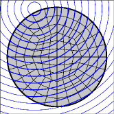
(a) setup

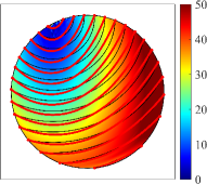
(b) result

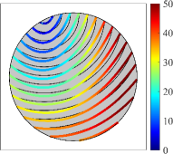
(c) result

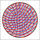
(d) result

Figure 10: Setup and results for test case 1 in 2D: (a) shows the bulk domain $\Omega_{\mathchoice{\displaystyle\boldsymbol{X}}{\textstyle\boldsymbol{X}}{\scriptstyle\boldsymbol{X}}{\scriptscriptstyle\boldsymbol{X}}}$ with selected level sets of $\phi\left(\mathchoice{\displaystyle\boldsymbol{X}}{\textstyle\boldsymbol{X}}{\scriptstyle\boldsymbol{X}}{\scriptscriptstyle\boldsymbol{X}}\right)$ and an example mesh used for the analysis, (b) shows the von Mises stress in $\Omega_{\mathchoice{\displaystyle\boldsymbol{x}}{\textstyle\boldsymbol{x}}{\scriptstyle\boldsymbol{x}}{\scriptscriptstyle\boldsymbol{x}}}$ and the deformed level sets in red, (c) is an alternative visualization with the same content where the von Mises stress is shown on the deformed level sets, (d) highlights the deformation of the bulk domain by showing elements in the undeformed and deformed meshes.

Figs. 10(b) to (d) show different visualizations obtained by a single analysis with the Bulk Trace FEM: (b) shows selected deformed level sets in red and von Mises stress obtained from the Cauchy stress tensor $\mathchoice{\displaystyle\boldsymbol{\sigma}}{\textstyle\boldsymbol{\sigma}}{\scriptstyle\boldsymbol{\sigma}}{\scriptscriptstyle\boldsymbol{\sigma}}$ in the deformed bulk domain as a color field, (c) is an alternative visualization where the von Mises stress is plotted on the deformed level sets themselves; doing this for all level sets would result in the color field shown in (b). Finally, Fig. 10(d) shows the elements of an example mesh in the undeformed and deformed bulk domain and the deformed level sets in red.

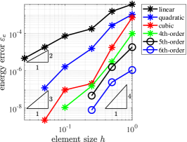
(a) convergence in $\varepsilon_{\mathfrak{e}}$

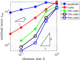
(b) convergence in $\varepsilon_{\mathrm{res}}$

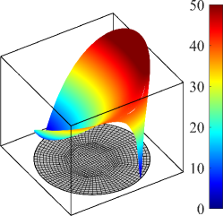
(c) von Mises stress

Figure 11: Convergence results for test case 1 in 2D: (a) and (b) show sub-optimal convergence rates in $\varepsilon_{\mathfrak{e}}$ and $\varepsilon_{\mathrm{res}}$, (c) shows the von Mises stress in the domain confirming locally steep gradients causing the sub-optimal results.

In the numerical analyses based on the Bulk Trace FEM, we have used sequences of meshes with different resolution and order (from 1 to 6), enabling systematic convergence studies in the error measures introduced above. Convergence results are seen in Fig. 11(a) for the stored energy error $\varepsilon_{\mathfrak{e}}$ and (b) for the residual error $\varepsilon_{\mathrm{res}}$. It is seen that for this test case, the convergence is sub-optimal because of locally steep gradients in the mechanical fields as shown for the example of the resulting von Mises stress field in Fig. 11(c).

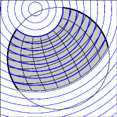
(a) setup

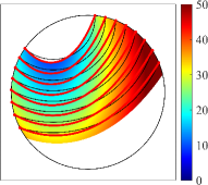
(b) result

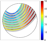
(c) result

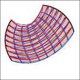
(d) result

Figure 12: Setup and results for test case 1 in 2D in the prescribed interval $\phi\in\left[-0.15,0.15\right]$.

Therefore, the analysis is now restricted to the level-set interval $\phi\in\left[-0.15,0.15\right]$ resulting in a subset of the previous domain as shown in Fig. 12(a) including an example mesh. Some results obtained with this mesh are visualized in Figs. 12(b) to (d) following the style of Fig. 10; all mechanical fields are smooth in this interval. The reference values for the integrated level sets are $\mathfrak{D}\left(\mathchoice{\displaystyle\boldsymbol{u}}{\textstyle\boldsymbol{u}}{\scriptstyle\boldsymbol{u}}{\scriptscriptstyle\boldsymbol{u}}\right)=0.1644415441226$ and for the stored elastic energy $\mathfrak{e}\left(\mathchoice{\displaystyle\boldsymbol{u}}{\textstyle\boldsymbol{u}}{\scriptstyle\boldsymbol{u}}{\scriptscriptstyle\boldsymbol{u}}\right)=7.792649686407\cdot 10^{-3}$. Convergence results are seen in Fig. 13 in all three error measures defined above. As can be seen, we obtain at least $p+1$ in $\varepsilon_{\phi}$ and $\varepsilon_{\mathfrak{e}}$, and $p-1$ in the residual error $\varepsilon_{\mathrm{res}}$ as expected. In Fig. 13(a), one can see that even element orders achieve $p+2$ in $\varepsilon_{\phi}$, whereas odd orders achieve $p+1$, which is also confirmed in the next test cases. In Fig. 13(b) one can see an even better convergence in the stored energy error $\varepsilon_{\mathfrak{e}}$, however, this can be traced back to the special case of using circular undeformed ropes as implied by Eq. (5.7). Using more general definitions rather leads to the expected rates of $p+1$, which is also confirmed in the next studies. Note that for the residual error shown in Fig. 13(c), the results obtained with linear meshes are omitted because they cannot be expected to converge as the expected rate is $p-1$ due to the involved second-order derivatives in $\varepsilon_{\mathrm{res}}$.

(a) convergence in $\varepsilon_{\phi}$

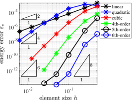
(b) convergence in $\varepsilon_{\mathfrak{e}}$

(c) convergence in $\varepsilon_{\mathrm{res}}$

Figure 13: Convergence results for test case 1 in 2D in the interval $\phi\in\left[-0.15,0.15\right]$ confirming optimal convergence rates in $\varepsilon_{\phi}$, $\varepsilon_{\mathfrak{e}}$ , and $\varepsilon_{\mathrm{res}}$.

Finally, a small experiment is described to confirm that the computed results are mechanically meaningful. Therefore, we select 10 level sets $\Gamma_{\!\!\mathchoice{\displaystyle\boldsymbol{X}}{\textstyle\boldsymbol{X}}{\scriptstyle\boldsymbol{X}}{\scriptscriptstyle\boldsymbol{X}}}^{c}$ of Eq. (5.7) with

$$c=\left\{-0.22,-0.19,-0.13,-0.07,-0.01,0.06,0.11,0.183,0.23,0.27\right\},$$

compute the corresponding arc lengths in the undeformed configuration and cut 10 chains with the respective lengths. The resulting displacement field is computed by means of the Bulk Trace FEM with largely increased $E$ (because the elastic strains in the chains under dead load are negligible). The computed deformed level sets are printed out true to scale and fixed to a board, see the green lines in Fig. 14(a). The chains are fixed with small nails at the corresponding end points of the level sets $\partial\Gamma_{\!\!\mathchoice{\displaystyle\boldsymbol{X}}{\textstyle\boldsymbol{X}}{\scriptstyle\boldsymbol{X}}{\scriptscriptstyle\boldsymbol{X}}}^{c}$, see Figs. 14(a) and (b) for the board lying horizontally. Then, the board is set vertically so that the chains deform under their own weight. The chains hang in the shape of catenaries as expected and are perfectly on top of the deformed level sets predicted with the Bulk Trace FEM, see Figs. 14(c) and (d). This is just to confirm that although the overall setup discussed in this work is rather unusual, the results are just as physically meaningful as any other mechanical model.

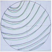
(a) front view, undef.

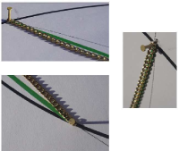
(b) zoom

(c) front view, def.

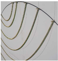
(d) side view, def.

Figure 14: Small-scale experiment to confirm that the Bulk Trace FEM is able to simultaneously capture the expected catenaries in the geometrical setup of test case 1 in 2D.

5.2 Test case 2 in 2D: Implicit bulk domain

Next, a more general shape of the bulk domain and level sets is suggested. The bulk domain $\Omega_{\mathchoice{\displaystyle\boldsymbol{X}}{\textstyle\boldsymbol{X}}{\scriptstyle\boldsymbol{X}}{\scriptscriptstyle\boldsymbol{X}}}$ is defined implicitly by the zero-level set of

$$\psi\left(\mathchoice{\displaystyle\boldsymbol{X}}{\textstyle\boldsymbol{X}}{\scriptstyle\boldsymbol{X}}{\scriptscriptstyle\boldsymbol{X}}\right)= \psi_{1}\left(\mathchoice{\displaystyle\boldsymbol{X}}{\textstyle\boldsymbol{X}}{\scriptstyle\boldsymbol{X}}{\scriptscriptstyle\boldsymbol{X}}\right)+\psi_{2}\left(\mathchoice{\displaystyle\boldsymbol{X}}{\textstyle\boldsymbol{X}}{\scriptstyle\boldsymbol{X}}{\scriptscriptstyle\boldsymbol{X}}\right)$$

$$\text{with }\;\psi_{1}\left(\mathchoice{\displaystyle\boldsymbol{X}}{\textstyle\boldsymbol{X}}{\scriptstyle\boldsymbol{X}}{\scriptscriptstyle\boldsymbol{X}}\right)= \left(\frac{X}{R_{X}}\right)^{2}+\left(\frac{Y}{R_{Y}}\right)^{2}-1,\quad R_{X}=10,\;R_{Y}=6.5,$$

$$\text{and }\;\psi_{2}\left(\mathchoice{\displaystyle\boldsymbol{X}}{\textstyle\boldsymbol{X}}{\scriptstyle\boldsymbol{X}}{\scriptscriptstyle\boldsymbol{X}}\right)= f_{\text{Bell}}\left(a\right).$$

Therein, $f_{\text{Bell}}$ is a $C_{4}$-continuous bell-shaped function defined as

$$f_{\text{Bell}}\left(a\right)= \begin{cases}\begin{array}[]{c}-1024\cdot a^{10}+5120\cdot a^{9}-10240\cdot a^{8}+\\ 10240\cdot a^{7}-5120\cdot a^{6}+1024\cdot a^{5}\end{array}&0\leq a\leq 1,\\ \;0&\text{else},\end{cases}$$

$$\text{with }\;a= \;\frac{r+R_{B}}{2\cdot R_{B}}\quad\text{and}\quad r=\left\|\mathchoice{\displaystyle\boldsymbol{X}}{\textstyle\boldsymbol{X}}{\scriptstyle\boldsymbol{X}}{\scriptscriptstyle\boldsymbol{X}}-\mathchoice{\displaystyle\boldsymbol{X}}{\textstyle\boldsymbol{X}}{\scriptstyle\boldsymbol{X}}{\scriptscriptstyle\boldsymbol{X}}_{B}\right\|.$$

In this example, $\mathchoice{\displaystyle\boldsymbol{X}}{\textstyle\boldsymbol{X}}{\scriptstyle\boldsymbol{X}}{\scriptscriptstyle\boldsymbol{X}}_{\!B}=\left[4,5\right]^{\mathrm{T}}$ and $R_{B}=12$. The resulting boundary of the implied bulk domain $\Omega_{\mathchoice{\displaystyle\boldsymbol{X}}{\textstyle\boldsymbol{X}}{\scriptstyle\boldsymbol{X}}{\scriptscriptstyle\boldsymbol{X}}}$, being the zero-level set of $\psi\left(\mathchoice{\displaystyle\boldsymbol{X}}{\textstyle\boldsymbol{X}}{\scriptstyle\boldsymbol{X}}{\scriptscriptstyle\boldsymbol{X}}\right)$, is the black line in Fig. 15(a). For the level-set function $\phi\left(\mathchoice{\displaystyle\boldsymbol{X}}{\textstyle\boldsymbol{X}}{\scriptstyle\boldsymbol{X}}{\scriptscriptstyle\boldsymbol{X}}\right)$ implying the geometries of interest, i.e., the undeformed ropes, we define

$$\phi\left(\mathchoice{\displaystyle\boldsymbol{X}}{\textstyle\boldsymbol{X}}{\scriptstyle\boldsymbol{X}}{\scriptscriptstyle\boldsymbol{X}}\right)= \;\nicefrac{{1}}{{2}}\left\|\mathchoice{\displaystyle\boldsymbol{X}}{\textstyle\boldsymbol{X}}{\scriptstyle\boldsymbol{X}}{\scriptscriptstyle\boldsymbol{X}}-\mathchoice{\displaystyle\boldsymbol{X}}{\textstyle\boldsymbol{X}}{\scriptstyle\boldsymbol{X}}{\scriptscriptstyle\boldsymbol{X}}_{F}\right\|-\nicefrac{{1}}{{10}}\cdot\sin\left(8\cdot\theta\left(\mathchoice{\displaystyle\boldsymbol{X}}{\textstyle\boldsymbol{X}}{\scriptstyle\boldsymbol{X}}{\scriptscriptstyle\boldsymbol{X}}\right)\right)-\nicefrac{{1}}{{2}},$$

$$\text{with }\;\theta\left(\mathchoice{\displaystyle\boldsymbol{X}}{\textstyle\boldsymbol{X}}{\scriptstyle\boldsymbol{X}}{\scriptscriptstyle\boldsymbol{X}}\right)= \;\text{atan}\frac{Y-Y_{F}}{X-X_{F}}\quad\text{and}\quad\mathchoice{\displaystyle\boldsymbol{X}}{\textstyle\boldsymbol{X}}{\scriptstyle\boldsymbol{X}}{\scriptscriptstyle\boldsymbol{X}}_{\!F}=\left[-10,10\right]^{\mathrm{T}},$$

see the blue lines in Fig. 15(a). Finally, the bulk domain of interest is defined as

$$\Omega_{\mathchoice{\displaystyle\boldsymbol{X}}{\textstyle\boldsymbol{X}}{\scriptstyle\boldsymbol{X}}{\scriptscriptstyle\boldsymbol{X}}}=\left\{\mathchoice{\displaystyle\boldsymbol{X}}{\textstyle\boldsymbol{X}}{\scriptstyle\boldsymbol{X}}{\scriptscriptstyle\boldsymbol{X}}\in\mathbb{R}^{2}:\psi\left(\mathchoice{\displaystyle\boldsymbol{X}}{\textstyle\boldsymbol{X}}{\scriptstyle\boldsymbol{X}}{\scriptscriptstyle\boldsymbol{X}}\right)\leq 0\;\;\text{and}\;\;4\leq\phi(\mathchoice{\displaystyle\boldsymbol{X}}{\textstyle\boldsymbol{X}}{\scriptstyle\boldsymbol{X}}{\scriptscriptstyle\boldsymbol{X}})\leq 7\right\}$$

and is shown in Fig. 15(b) with an example mesh and selected level sets of $\phi\left(\mathchoice{\displaystyle\boldsymbol{X}}{\textstyle\boldsymbol{X}}{\scriptstyle\boldsymbol{X}}{\scriptscriptstyle\boldsymbol{X}}\right)$.

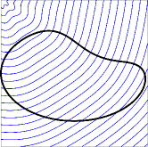
(a) level sets

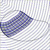
(b) $\Omega_{\mathchoice{\displaystyle\boldsymbol{X}}{\textstyle\boldsymbol{X}}{\scriptstyle\boldsymbol{X}}{\scriptscriptstyle\boldsymbol{X}}}$ and mesh

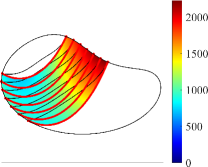
(c) result

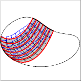
(d) result

Figure 15: Setup and results for test case 2 in 2D in the prescribed interval $\phi\in\left[4,7\right]$.

Material parameters are again set to $E=10\,000$ and the bulk forces are $\mathchoice{\displaystyle\boldsymbol{F}}{\textstyle\boldsymbol{F}}{\scriptstyle\boldsymbol{F}}{\scriptscriptstyle\boldsymbol{F}}\!\left(\mathchoice{\displaystyle\boldsymbol{X}}{\textstyle\boldsymbol{X}}{\scriptstyle\boldsymbol{X}}{\scriptscriptstyle\boldsymbol{X}}\right)=\left[0,-200\right]^{\mathrm{T}}$. Zero displacements are prescribed on $\partial\Omega_{\mathchoice{\displaystyle\boldsymbol{X}}{\textstyle\boldsymbol{X}}{\scriptstyle\boldsymbol{X}}{\scriptscriptstyle\boldsymbol{X}}}$. Benchmark values for the integrated level sets are $\mathfrak{D}\left(\mathchoice{\displaystyle\boldsymbol{u}}{\textstyle\boldsymbol{u}}{\scriptstyle\boldsymbol{u}}{\scriptscriptstyle\boldsymbol{u}}\right)=39.05000466379$ and for the stored energy $\mathfrak{e}\left(\mathchoice{\displaystyle\boldsymbol{u}}{\textstyle\boldsymbol{u}}{\scriptstyle\boldsymbol{u}}{\scriptscriptstyle\boldsymbol{u}}\right)=2317.129363166$. The deformed bulk domain $\Omega_{\mathchoice{\displaystyle\boldsymbol{x}}{\textstyle\boldsymbol{x}}{\scriptstyle\boldsymbol{x}}{\scriptscriptstyle\boldsymbol{x}}}$ is seen in Fig. 15(c) and (d). Convergence results are seen in Fig. 16 in all three error measures. The convergence in $\varepsilon_{\phi}$ and $\varepsilon_{\mathfrak{e}}$ is $p+1$ for odd element orders and $p+2$ for even orders. The convergence in $\varepsilon_{\mathrm{res}}$ is $p-1$ as expected. The same rates of convergence have been obtained using triangular and quadrilateral elements in the Bulk Trace FEM analyses, respectively.

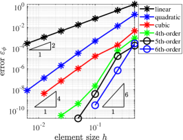
(a) convergence in $\varepsilon_{\phi}$

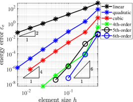
(b) convergence in $\varepsilon_{\mathfrak{e}}$

(c) convergence in $\varepsilon_{\mathrm{res}}$

Figure 16: Convergence results for test case 2 in 2D confirming optimal convergence rates in $\varepsilon_{\phi}$, $\varepsilon_{\mathfrak{e}}$ , and $\varepsilon_{\mathrm{res}}$.

5.3 Test case 3 in 3D: Spherical bulk domain

The bulk domain is a subset of a sphere with radius $1$ centered at the origin. Let $\psi\left(\mathchoice{\displaystyle\boldsymbol{X}}{\textstyle\boldsymbol{X}}{\scriptstyle\boldsymbol{X}}{\scriptscriptstyle\boldsymbol{X}}\right)=\left\|\mathchoice{\displaystyle\boldsymbol{X}}{\textstyle\boldsymbol{X}}{\scriptstyle\boldsymbol{X}}{\scriptscriptstyle\boldsymbol{X}}\right\|-1$ and $\phi\left(\mathchoice{\displaystyle\boldsymbol{X}}{\textstyle\boldsymbol{X}}{\scriptstyle\boldsymbol{X}}{\scriptscriptstyle\boldsymbol{X}}\right)=Z$, then

$$\Omega_{\mathchoice{\displaystyle\boldsymbol{X}}{\textstyle\boldsymbol{X}}{\scriptstyle\boldsymbol{X}}{\scriptscriptstyle\boldsymbol{X}}}=\left\{\mathchoice{\displaystyle\boldsymbol{X}}{\textstyle\boldsymbol{X}}{\scriptstyle\boldsymbol{X}}{\scriptscriptstyle\boldsymbol{X}}\in\mathbb{R}^{3}:\psi\left(\mathchoice{\displaystyle\boldsymbol{X}}{\textstyle\boldsymbol{X}}{\scriptstyle\boldsymbol{X}}{\scriptscriptstyle\boldsymbol{X}}\right)\leq 0\;\;\text{and}\;\;-\nicefrac{{1}}{{5}}\leq\phi(\mathchoice{\displaystyle\boldsymbol{X}}{\textstyle\boldsymbol{X}}{\scriptstyle\boldsymbol{X}}{\scriptscriptstyle\boldsymbol{X}})\leq\nicefrac{{2}}{{5}}\right\}.$$

The resulting undeformed bulk domain is seen in Fig. 17(a) and an example mesh in (b). It can also be seen that a set of planar and circular membranes is implied in the undeformed configuration. The thickness of the membranes is $t=1$, Young’s modulus is $E=1\,000$ and Poisson ratio $\nu=0.3$, which is easily converted into the Lamé parameters. The loading is gravity acting on the membrane surfaces with $\mathchoice{\displaystyle\boldsymbol{F}}{\textstyle\boldsymbol{F}}{\scriptstyle\boldsymbol{F}}{\scriptscriptstyle\boldsymbol{F}}\!\left(\mathchoice{\displaystyle\boldsymbol{X}}{\textstyle\boldsymbol{X}}{\scriptstyle\boldsymbol{X}}{\scriptscriptstyle\boldsymbol{X}}\right)=\left[0,0,-100\right]^{\mathrm{T}}$ for all $\mathchoice{\displaystyle\boldsymbol{X}}{\textstyle\boldsymbol{X}}{\scriptstyle\boldsymbol{X}}{\scriptscriptstyle\boldsymbol{X}}\in\Omega_{\!\mathchoice{\displaystyle\boldsymbol{X}}{\textstyle\boldsymbol{X}}{\scriptstyle\boldsymbol{X}}{\scriptscriptstyle\boldsymbol{X}}}$. The whole boundary is treated as a Dirichlet boundary with prescribed zero-displacements.

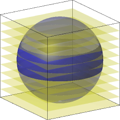
(a) level sets

      

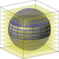
(b) $\Omega_{\mathchoice{\displaystyle\boldsymbol{X}}{\textstyle\boldsymbol{X}}{\scriptstyle\boldsymbol{X}}{\scriptscriptstyle\boldsymbol{X}}}$ and mesh

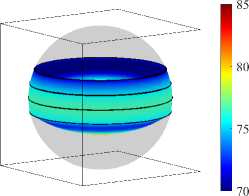
(c) result

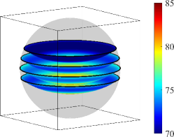
(d) result

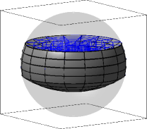
(e) result

Figure 17: Setup and results for test case 3 in 3D in the prescribed interval $\phi\in\left[-\nicefrac{{1}}{{5}},\nicefrac{{2}}{{5}}\right]$.

Results of a single analysis are seen in Figs. 17(c) to (e); (c) and (d) are alternative visualizations of the von Mises stress based on $\mathchoice{\displaystyle\boldsymbol{\sigma}}{\textstyle\boldsymbol{\sigma}}{\scriptstyle\boldsymbol{\sigma}}{\scriptscriptstyle\boldsymbol{\sigma}}$, once shown on the boundary $\partial\Omega_{\mathchoice{\displaystyle\boldsymbol{x}}{\textstyle\boldsymbol{x}}{\scriptstyle\boldsymbol{x}}{\scriptscriptstyle\boldsymbol{x}}}$ and once on selected level sets $\Gamma_{\!\!\mathchoice{\displaystyle\boldsymbol{x}}{\textstyle\boldsymbol{x}}{\scriptstyle\boldsymbol{x}}{\scriptscriptstyle\boldsymbol{x}}}^{c}$ with $c\in\left\{-\nicefrac{{1}}{{5}},0,\nicefrac{{1}}{{5}},\nicefrac{{2}}{{5}}\right\}$. Convergence results are seen in Fig. 18. Therefore, benchmark values of $\mathfrak{D}\left(\mathchoice{\displaystyle\boldsymbol{u}}{\textstyle\boldsymbol{u}}{\scriptstyle\boldsymbol{u}}{\scriptscriptstyle\boldsymbol{u}}\right)=1.981355380281$ and $\mathfrak{e}\left(\mathchoice{\displaystyle\boldsymbol{u}}{\textstyle\boldsymbol{u}}{\scriptstyle\boldsymbol{u}}{\scriptscriptstyle\boldsymbol{u}}\right)=6.588725461796$ have been used to compute $\varepsilon_{\phi}$ and $\varepsilon_{\mathfrak{e}}$; in three dimensions, $\varepsilon_{\phi}$ is the error in the integrated areas of the level sets over the deformed bulk domain. As can be seen, optimal results are again achieved in all three error measures. For $\varepsilon_{\phi}$ and $\varepsilon_{\mathfrak{e}}$, we again confirm $p+1$ for odd element orders and $p+2$ for even orders.

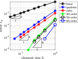
(a) convergence in $\varepsilon_{\phi}$

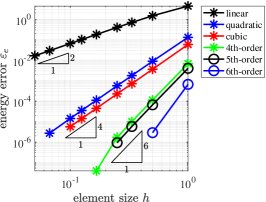
(b) convergence in $\varepsilon_{\mathfrak{e}}$

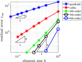
(c) convergence in $\varepsilon_{\mathrm{res}}$

Figure 18: Convergence results for test case 1 in 3D confirming optimal convergence rates in $\varepsilon_{\phi}$, $\varepsilon_{\mathfrak{e}}$ , and $\varepsilon_{\mathrm{res}}$.

5.4 Test case 4 in 3D: Ellipsoidal bulk domain

We define the two level-set functions

$$\psi\left(\mathchoice{\displaystyle\boldsymbol{X}}{\textstyle\boldsymbol{X}}{\scriptstyle\boldsymbol{X}}{\scriptscriptstyle\boldsymbol{X}}\right)=\left(\frac{X-X_{E}}{R_{X}}\right)^{2}+\left(\frac{Y-Y_{E}}{R_{Y}}\right)^{2}+\left(\frac{Z-Z_{E}}{R_{Z}}\right)^{2}-1,$$

with $\mathchoice{\displaystyle\boldsymbol{X}}{\textstyle\boldsymbol{X}}{\scriptstyle\boldsymbol{X}}{\scriptscriptstyle\boldsymbol{X}}_{\!E}=\left[-0.2,0.2,0.1\right]^{\mathrm{T}}$ and $R_{X}=0.9$, $R_{Y}=0.7$, $R_{Z}=0.8$ and

$$\phi\left(\mathchoice{\displaystyle\boldsymbol{X}}{\textstyle\boldsymbol{X}}{\scriptstyle\boldsymbol{X}}{\scriptscriptstyle\boldsymbol{X}}\right)=\left\|\mathchoice{\displaystyle\boldsymbol{X}}{\textstyle\boldsymbol{X}}{\scriptstyle\boldsymbol{X}}{\scriptscriptstyle\boldsymbol{X}}-\mathchoice{\displaystyle\boldsymbol{X}}{\textstyle\boldsymbol{X}}{\scriptstyle\boldsymbol{X}}{\scriptscriptstyle\boldsymbol{X}}_{\!S}\right\|-R_{S}$$

with $\mathchoice{\displaystyle\boldsymbol{X}}{\textstyle\boldsymbol{X}}{\scriptstyle\boldsymbol{X}}{\scriptscriptstyle\boldsymbol{X}}_{\!S}=\left[-1,1,2\right]^{\mathrm{T}}$ and $R_{S}=2$, see Fig. 19(a). The bulk domain is defined as

$$\Omega_{\mathchoice{\displaystyle\boldsymbol{X}}{\textstyle\boldsymbol{X}}{\scriptstyle\boldsymbol{X}}{\scriptscriptstyle\boldsymbol{X}}}=\left\{\mathchoice{\displaystyle\boldsymbol{X}}{\textstyle\boldsymbol{X}}{\scriptstyle\boldsymbol{X}}{\scriptscriptstyle\boldsymbol{X}}\in\mathbb{R}^{3}:\psi\left(\mathchoice{\displaystyle\boldsymbol{X}}{\textstyle\boldsymbol{X}}{\scriptstyle\boldsymbol{X}}{\scriptscriptstyle\boldsymbol{X}}\right)\leq 0\;\;\text{and}\;\;0\leq\phi(\mathchoice{\displaystyle\boldsymbol{X}}{\textstyle\boldsymbol{X}}{\scriptstyle\boldsymbol{X}}{\scriptscriptstyle\boldsymbol{X}})\leq\nicefrac{{1}}{{2}}\right\}.$$

The resulting undeformed bulk domain with an example mesh is seen in Fig. 19(b). All material parameters, loading and boundary conditions are given as in the previous test case in Section 5.3. Results are seen in Figs. 19(c) and (d) following previous visualizations. Benchmark values for the convergence studies are $\mathfrak{D}\left(\mathchoice{\displaystyle\boldsymbol{u}}{\textstyle\boldsymbol{u}}{\scriptstyle\boldsymbol{u}}{\scriptscriptstyle\boldsymbol{u}}\right)=1.032907088507$ and $\mathfrak{e}\left(\mathchoice{\displaystyle\boldsymbol{u}}{\textstyle\boldsymbol{u}}{\scriptstyle\boldsymbol{u}}{\scriptscriptstyle\boldsymbol{u}}\right)=1.863258461070$. However, because the resulting convergence plots are virtually identical to previous test cases, only the convergence in the stored energy error $\varepsilon_{\mathfrak{e}}$ is shown in Fig. 19(e).

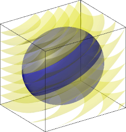
(a) level sets

      

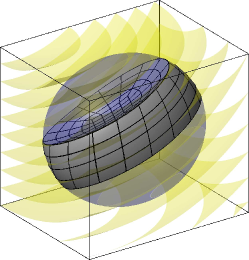
(b) $\Omega_{\mathchoice{\displaystyle\boldsymbol{X}}{\textstyle\boldsymbol{X}}{\scriptstyle\boldsymbol{X}}{\scriptscriptstyle\boldsymbol{X}}}$ and mesh

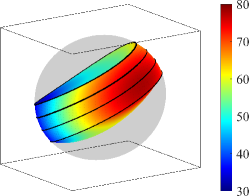
(c) result

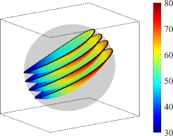
(d) result

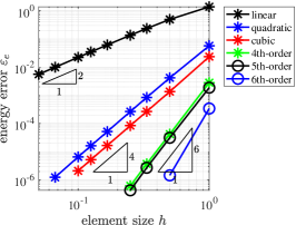
(e) convergence

Figure 19: Setup and results for test case 4 in 3D in the prescribed interval $\phi\in\left[0,\nicefrac{{1}}{{2}}\right]$.

5.5 Test case 5 in 2D: Bulk material with embedded fibres

The final example considers a coupled problem where some isotropic and homogeneous bulk material is reinforced with curved, one-dimensional fibres. This application relates to the discussion of continuously embedded sub-structure models in Section 3.7. The bulk domain is a quarter annulus centered at the origin, an inner radius of $R_{i}=8$ and an outer radius of $R_{o}=12$, see Fig. 20(a). The resulting area is $A=\nicefrac{{1}}{{4}}\cdot\pi\cdot\left(R_{o}^{2}-R_{i}^{2}\right)=20\pi$. In contrast to the previous examples where the focus was exclusively on the behaviour of ropes and membranes within bulk domains, in this study, there is also an isotropic bulk material characterized by a Young’s modulus of $E_{b}=10\,000$ and a Poisson’s number of $\nu_{b}=0.3$; the Lamé constants are then computed according to plane strain conditions. The behaviour of the bulk material is modeled according to standard finite strain theory in two dimensions. There is a body force of $\mathchoice{\displaystyle\boldsymbol{F}}{\textstyle\boldsymbol{F}}{\scriptstyle\boldsymbol{F}}{\scriptscriptstyle\boldsymbol{F}}\!\left(\mathchoice{\displaystyle\boldsymbol{X}}{\textstyle\boldsymbol{X}}{\scriptstyle\boldsymbol{X}}{\scriptscriptstyle\boldsymbol{X}}\right)=\left[0,-20\right]^{\mathrm{T}}$ acting on the bulk material only (i.e., there are no additional body forces on the fibres). Zero-displacements are prescribed on the lower side of the bulk domain where $Y\!=0$.

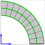
(a) $n_{\mathrm{rad}}=2$

(b) $n_{\mathrm{rad}}=3$

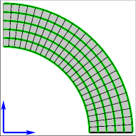
(c) $n_{\mathrm{rad}}=5$

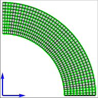
(d) $n_{\mathrm{rad}}=10$

Figure 20: Discrete fibre model in an annulus where the number of fibres (and their stiffness) is associated to the number of elements in radial direction $n_{\mathrm{rad}}$. The embedded fibres are meshed conformingly by the element edges shown as green lines.

For the modeling of the fibres, two strategies are compared: In the first approach, we consider a discrete set of fibres where the number of fibres is coupled to the element number used in the analysis, see Fig. 20. As can be seen, the discrete fibres are meshed conformingly by curved, one-dimensional elements and one may use standard approaches (i.e., classical Surface FEM) for the modeling and analysis, see, e.g., [5, 15, 20, 17, 36]; of course, coupled to the analysis of the bulk material. Let $n_{\mathrm{rad}}$ be the number of elements in radial direction of the annulus, then there are $n_{\mathrm{rad}}+1$ fibres with geometries $\Gamma_{\!\mathchoice{\displaystyle\boldsymbol{X}}{\textstyle\boldsymbol{X}}{\scriptstyle\boldsymbol{X}}{\scriptscriptstyle\boldsymbol{X}}}^{i}$, $i=1,\dots n_{\mathrm{rad}}+1$ in the analysis. In order not to make the fibre-reinforced annulus stiffer upon increasing the element number, we reduce the stiffness of the fibres with each refinement step. Therefore, it is useful to define a target value for the integrated Young’s modulus over the bulk domain and the fibres as

$$\int_{\Omega_{\mathchoice{\displaystyle\boldsymbol{X}}{\textstyle\boldsymbol{X}}{\scriptstyle\boldsymbol{X}}{\scriptscriptstyle\boldsymbol{X}}}}E_{b}\;\mathrm{d}\Omega+\sum_{i=1}^{n_{\mathrm{rad}}+1}\int_{\Gamma_{\!\mathchoice{\displaystyle\boldsymbol{X}}{\textstyle\boldsymbol{X}}{\scriptstyle\boldsymbol{X}}{\scriptscriptstyle\boldsymbol{X}}}^{i}}E_{\mathrm{discr}}\;\mathrm{d}\Omega =580\,000\pi,$$

$$\Rightarrow\sum_{i=1}^{n_{\mathrm{rad}}+1}\int_{\Gamma_{\!\mathchoice{\displaystyle\boldsymbol{X}}{\textstyle\boldsymbol{X}}{\scriptstyle\boldsymbol{X}}{\scriptscriptstyle\boldsymbol{X}}}^{i}}E_{\mathrm{discr}}\;\mathrm{d}\Omega =580\,000\pi-20\pi\cdot 10\,000,$$

$$\Rightarrow E_{\mathrm{discr}} =76\,000\,/\,\left(n_{\mathrm{rad}}+1\right).$$

This enables us to keep the cross section of the fibres at $1$. Of course, one could also define a constant Young’s modulus for the discrete fibres and adjust the cross section with respect to $n_{\mathrm{rad}}$. Note that the Poisson number plays no role for fibres, hence, $\nu=0$. A sketch of the deformed domain may be seen in Fig. 21(a).

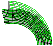
(a) deformation

            

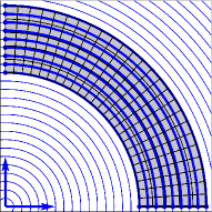
(b) cont. fibre model

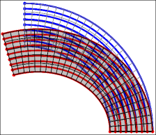
(c) deformation

Figure 21: (a) shows the deformed configuration according to the discrete fibre model with $n_{\mathrm{rad}}=10$, (b) shows the continuous fibre model in an annulus where the fibres are implied by all level sets in the interval $\phi\in\left[8,12\right]$, (c) is the deformed configuration for the continuous fibre model as obtained with the Bulk Trace FEM.

The other strategy for the fibres is to associate a continuous set of fibres to the level sets of $\phi\left(\mathchoice{\displaystyle\boldsymbol{X}}{\textstyle\boldsymbol{X}}{\scriptstyle\boldsymbol{X}}{\scriptscriptstyle\boldsymbol{X}}\right)=\left\|\mathchoice{\displaystyle\boldsymbol{X}}{\textstyle\boldsymbol{X}}{\scriptstyle\boldsymbol{X}}{\scriptscriptstyle\boldsymbol{X}}\right\|$ in the interval $\phi_{\min}=8$ and $\phi_{\max}=12$, see Fig. 21(b), as proposed in this work. Then, the Young’s modulus is computed as

$$\int_{\Omega_{\mathchoice{\displaystyle\boldsymbol{X}}{\textstyle\boldsymbol{X}}{\scriptstyle\boldsymbol{X}}{\scriptscriptstyle\boldsymbol{X}}}}E_{b}\;\mathrm{d}\Omega+\int_{\Omega_{\mathchoice{\displaystyle\boldsymbol{X}}{\textstyle\boldsymbol{X}}{\scriptstyle\boldsymbol{X}}{\scriptscriptstyle\boldsymbol{X}}}}E_{\mathrm{cont}}\cdot\left\|\nabla_{\!\!\mathchoice{\displaystyle\boldsymbol{X}}{\textstyle\boldsymbol{X}}{\scriptstyle\boldsymbol{X}}{\scriptscriptstyle\boldsymbol{X}}}\phi\right\|\;\mathrm{d}\Omega =580\,000\pi,$$

$$\Rightarrow E_{\mathrm{cont}}\cdot 20\pi =580\,000\pi-20\pi\cdot 10\,000,$$

$$\Rightarrow E_{\mathrm{cont}} =19\,000,$$

keeping the cross section constant at $1$. Together with $\nu=0$, these material parameters are used for the analysis based on the Bulk Trace FEM as outlined above, this time coupled with the classical 2D analysis of the bulk material. The deformed domain, obtained with the Bulk Trace FEM, is shown in Fig. 21(c). We observe a stored elastic energy of $\mathfrak{e}\left(\mathchoice{\displaystyle\boldsymbol{u}}{\textstyle\boldsymbol{u}}{\scriptstyle\boldsymbol{u}}{\scriptscriptstyle\boldsymbol{u}}\right)=674.363$ and a displacement of the lower left node as $\mathchoice{\displaystyle\boldsymbol{u}}{\textstyle\boldsymbol{u}}{\scriptstyle\boldsymbol{u}}{\scriptscriptstyle\boldsymbol{u}}\left(0,8\right)=\left[-1.0194534,-2.710712\right]^{\mathrm{T}}$. Most importantly, we confirm that the strategy based on the discrete fibres converges to the case of continuous fibres as proposed herein. However, it is also important to note that due to the boundary conditions, there is a singularity at the corner points at $\mathchoice{\displaystyle\boldsymbol{X}}{\textstyle\boldsymbol{X}}{\scriptstyle\boldsymbol{X}}{\scriptscriptstyle\boldsymbol{X}}=\left[8,0\right]^{\mathrm{T}}$ and $\left[12,0\right]^{\mathrm{T}}$ which hinders optimal convergence rates. Therefore, these results are given with reduced accuracy compared to the previous test cases.

In order to make the results more quantifiable, it was found useful to provide energy results for a prescribed displacement field of

$$\mathchoice{\displaystyle\boldsymbol{u}}{\textstyle\boldsymbol{u}}{\scriptstyle\boldsymbol{u}}{\scriptscriptstyle\boldsymbol{u}}\left(\mathchoice{\displaystyle\boldsymbol{X}}{\textstyle\boldsymbol{X}}{\scriptstyle\boldsymbol{X}}{\scriptscriptstyle\boldsymbol{X}}\right)=\left[\begin{array}[]{c}u\left(X,Y\right)\\ v\left(X,Y\right)\end{array}\right]=\left[\begin{array}[]{c}\nicefrac{{1}}{{2}}\sin\left(\nicefrac{{1}}{{2}}Y\right)\\ \nicefrac{{1}}{{10}}\sin\left(Y\right)\end{array}\right],$$ (5.9)

see Fig. 22(a). Then, a benchmark energy for the scenario with continuously embedded fibres may be provided with $\mathfrak{e}\left(\mathchoice{\displaystyle\boldsymbol{u}}{\textstyle\boldsymbol{u}}{\scriptstyle\boldsymbol{u}}{\scriptscriptstyle\boldsymbol{u}}\right)=11499.322459892$ with high accuracy. The Bulk Trace FEM converges with optimal accuracy to this benchmark value, see Fig. 22(b). It can also be confirmed that the discrete-fibre setting converges to this energy as seen in Fig. 22(c). However, one may then only expect a first-order convergence (independently of the element orders) due to the different geometric representation of the fibres. It is thus confirmed that the proposed modeling and analysis of structures implied by all level sets within a bulk domain provides the basis for continuously embedded sub-structure models within (isotropic) bulk materials which will be further investigated in future works.

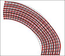
(a) prescribed displ.

            

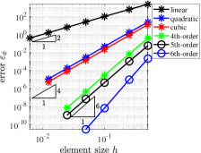
(b) cont. fibre model

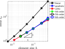
(c) discrete fibre model

Figure 22: (a) shows the deformed configuration according to the prescribed displacement field in Eq. (5.9), (b) shows convergence rates for the continuous fibre model and (c) for the discrete fibre model towards the reference energy of the continuous model.

6 Conclusions

A mechanical model for structural ropes and membranes is formulated which simultaneously applies to all level sets in a bulk domain. Interpreting the level sets in the undeformed and deformed bulk domains yields the material and spatial configurations of the (curved) structures. For the modeling, it is crucial to employ classical differential operators with respect to the bulk domain as well as surface differential operators with respect to the level sets. Then, all mechanical quantities such as displacements, stresses and strains may be specified accordingly. The resulting BVP in strong form may be reformulated in weak form using the co-area formula and the divergence theorem on manifolds, resulting in integral terms over the bulk domain.

For the numerical analysis, one may then employ a (higher-order) mesh in the bulk domain which conforms to the boundaries of the bulk domain, however, it does (typically) not conform to the geometry of the level-set structures. This method is called the Bulk Trace FEM as it features similarities to the classical FEM with conforming meshes and the Trace FEM using non-conforming meshes. Most importantly, the Bulk Trace FEM does not feature cut elements and, therefore, standard methods for the numerical integration and enforcement of boundary conditions may be employed without any need for stabilization. Technical aspects of the implementation are outlined and enable a straightforward implementation of the method in an existing FE solver.

The numerical results confirm that higher-order convergence rates are achieved as expected. The potential of the proposed method for the simultaneous assessment of mechanical properties of structures implied by all level sets in a bulk domain is shown. Furthermore, the described model may easily be combined with conventional (mechanical) bulk models for $d$-dimensional structures, introducing a new concept for advanced material models, possibly labelled continuously embedded sub-structure models or embedded, layered manifold models. In future works, we shall extend the present approach for membranes also to classical theories of shells with the same motivation to enable the simultaneous analysis of shells on all level sets in a bulk domain or to add sub-structures to existing bulk materials.

References

- [1] Abedian, A.; Parvizian, J.; Düster, A.; Khademyzadeh, H.; Rank, E.: Performance of different integration schemes in facing discontinuities in the Finite Cell Method. International Journal of Computational Methods, 10, 1–24, 2013.
- [2] Adalsteinsson, D.; Sethian, J.A.: Transport and diffusion of material quantities on propagating interfaces via level set methods. J. Comput. Phys., 185, 271–288, 2003.
- [3] Belytschko, T.; Liu, W.K.; Moran, B.: Nonlinear Finite Elements for Continua and Structures. John Wiley & Sons, Chichester, 2000.
- [4] Bertalmio, M.; Cheng, L.T.; Osher, S.; Sapiro, G.: Variational problems and partial differential equations on implicit surfaces: The framework and examples in image processing and pattern formation. J. Comput. Phys., 174, 759–780, 2001.
- [5] Bischoff, M.; Ramm, E.; Irslinger., J.: Models and Finite Elements for Thin-Walled Structures. Encyclopedia of Computational Mechanics Second Edition (eds E. Stein, R. Borst and T. J. Hughes), John Wiley & Sons, Chichester, 2017.
- [6] Burger, M.: Finite element approximation of elliptic partial differential equations on implicit surfaces. Comput. Vis. Sci., 12, 87–100, 2009.
- [7] Burman, E.: A penalty-free nonsymmetric Nitsche-type method for the weak imposition of boundary conditions. SIAM J. Numer. Anal., 50, 1959–1981, 2012.
- [8] Burman, E.; Claus, S.; Hansbo, P.; Larson, M.G.; Massing, A.: CutFEM: Discretizing geometry and partial differential equations. Internat. J. Numer. Methods Engrg., 104, 472–501, 2015.
- [9] Burman, E.; Hansbo, P.: Fictitious domain finite element methods using cut elements: I. A stabilized Lagrange multiplier method. Comp. Methods Appl. Mech. Engrg., 199, 2680–2686, 2010.
- [10] Burman, E.; Hansbo, P.: Fictitious domain finite element methods using cut elements: II. A stabilized Nitsche method. Applied Numerical Mathematics, 62, 328–341, 2012.
- [11] Burman, E.; Hansbo, P.; Larson, M.G.: A stabilized cut finite element method for partial differential equations on surfaces: The Laplace-Beltrami operator. Comp. Methods Appl. Mech. Engrg., 285, 188–207, 2015.
- [12] Burman, E.; Hansbo, P.; Larson, M.G.: A simple finite element method for elliptic bulk problems with embedded surfaces. Comp. Geosciences, 23, 189–199, 2019.
- [13] Burman, E.; Hansbo, P.; Larson, M.G.; Massing, A.: Cut finite element methods for partial differential equations on embedded manifolds of arbitrary codimensions. ESAIM: Math. Model. Numer. Anal., 52, 2247–2282, 2018.
- [14] Burman, E.; Hansbo, P.; Larson, M.G.; Zahedi, S.: Stabilized CutFEM for the convection problem on surfaces. Numer. Math., 141, 103–139, 2019.
- [15] Calladine, C. R.: Theory of Shell Structures. Cambridge University Press, Cambridge, 1983.
- [16] Cenanovic, M.; Hansbo, P.; Larson, M.G.: Cut finite element modeling of linear membranes. Comp. Methods Appl. Mech. Engrg., 310, 98–111, 2016.
- [17] Chapelle, D.; Bathe, K.J.: The Finite Element Analysis of Shells – Fundamentals. Computational Fluid and Solid Mechanics. Springer, Berlin, 2011.
- [18] Cheng, K.W.; Fries, T.P.: Higher-order XFEM for curved strong and weak discontinuities. Internat. J. Numer. Methods Engrg., 82, 564–590, 2010.
- [19] Chernyshenko, A.Y.; Olshanskii, M.A.: An adaptive octree finite element method for PDEs posed on surfaces. Comp. Methods Appl. Mech. Engrg., 291, 146–172, 2015.
- [20] Ciarlet, P.G.: Mathematical Elasticity, III: Theory of Shells. Elsevier, Amsterdam, 1997.
- [21] Deckelnick, K.; Dziuk, G.; Elliott, C.M.; Heine, C.J.: An -narrow band finite-element method for elliptic equations on implicit surfaces. IMA J. Numer. Anal., 30, 351–376, 2010.
- [22] Deckelnick, K.; Elliott, C.M.; Ranner, T.: Unfitted finite element methods using bulk meshes for surface partial differential equations. SIAM J. Numer. Anal., 52, 2137–2162, 2014.
- [23] Delfour, M.C.; Zolésio, J.P.: Tangential Differential Equations for Dynamical Thin-Shallow Shells. Journal of Differential Equations, 128, 125–167, 1996.
- [24] Delfour, M.C.; Zolésio, J.P.: Shapes and geometries—Metrics, Analysis, Differential Calculus, and Optimization. SIAM, Philadelphia, PA, 2011.
- [25] do Carmo, M.P.: Differential geometry of curves and surfaces. Prentice-Hall, Englewood Cliffs, NJ, 1976.
- [26] Dziuk, G.; Elliott, C.M.: An Eulerian approach to transport and diffusion on evolving implicit surfaces. Comput. Vis. Sci., 13, 17–28, 2008.
- [27] Dziuk, G.; Elliott, C.M.: Eulerian finite element method for parabolic PDEs on implicit surfaces. Interfaces and Free Boundaries, 10, 2008.
- [28] Dziuk, G.; Elliott, C.M.: An Eulerian approach to transport and diffusion on evolving implicit surfaces. Computing and Visualization in Science, 13, 17–28, 2010.
- [29] Dziuk, G.; Elliott, C.M.: Finite element methods for surface PDEs. Acta Numerica, 22, 289–396, 2013.
- [30] Farin, G.E.: NURBS Curves and Surfaces: from Projective Geometry to Practical Use. A.K. Peters, Ltd., 6000 Broken Sound Parkway NW, 2 edition, 1999.
- [31] Federer, H.: Geometric measure theory. Springer, New York, 1969.
- [32] Fernández-Méndez, S.; Huerta, A.: Imposing essential boundary conditions in mesh-free methods. Comp. Methods Appl. Mech. Engrg., 193, 1257–1275, 2004.
- [33] Formaggia, L.; Fumagalli, A.; Scotti, A.; Ruffo, P.: A reduced model for Darcy’s problem in networks of fractures. ESAIM: Mathematical Modelling and Numerical Analysis, 48, 1089–1116, 2014.
- [34] Fries, T.P.; Omerović, S.: Higher-order accurate integration of implicit geometries. Internat. J. Numer. Methods Engrg., 106, 323–371, 2016.
- [35] Fries, T.P.; Omerović, S.; Schöllhammer, D.; Steidl, J.: Higher-order meshing of implicit geometries—part I: Integration and interpolation in cut elements. arXiv: 1706.00578, 2017.
- [36] Fries, T.P.; Schöllhammer, D.: A unified finite strain theory for membranes and ropes. Comp. Methods Appl. Mech. Engrg., 365, 113031, 2020.
- [37] Gfrerer, M.H.; Schanz, M.: A high-order FEM with exact geometry description for the Laplacian on implicitly defined surfaces. Internat. J. Numer. Methods Engrg., 114, 1163–1178, 2018.
- [38] Grande, J.; Lehrenfeld, C.; Reusken, A.: Analysis of a high-order trace finite element method for PDEs on level set surfaces. SIAM J. Numer. Anal., 56, 228–255, 2018.
- [39] Grande, J.; Reusken, A.: A Higher Order Finite Element Method for Partial Differential Equations on Surfaces. SIAM J. Numer. Anal., 54, 388–414, 2016.
- [40] Greer, J.B.: An Improvement of a Recent Eulerian Method for Solving PDEs on General Geometries. Journal of Scientific Computing, 29, 321–352, 2006.
- [41] Greer, J.B.; Bertozzi, A.L.; Sapiro, G.: Fourth order partial differential equations on general geometries. J. Comput. Phys., 216, 216–246, 2006.
- [42] Gross, S.; Jankuhn, T.; Olshanskii, M.A.; Reusken, A.: A trace finite element method for vector-Laplacians on surfaces. SIAM J. Numer. Anal., 56, 2406–2429, 2018.
- [43] Hansbo, P.; Larson, M.G.: Nitsche’s finite element method for model coupling in elasticity. Comp. Methods Appl. Mech. Engrg., 392, 114707, 2022.
- [44] Holzapfel, G.A.: Nonlinear Solid Mechanics: A Continuum Approach for Engineering. John Wiley & Sons, Chichester, 2000.
- [45] Ibrahimbegović, A.; Gruttmann, F.: A consistent finite element formulation of nonlinear membrane shell theory with particular reference to elastic rubberlike material. Finite Elem. Anal. Des., 13, 75–86, 1993.
- [46] Jankuhn, T.; Olshanskii, M.A.; Reusken, A.: Incompressible fluid problems on embedded surfaces: Modeling and variational formulations. Interfaces and Free Boundaries, 20, 353–377, 2018.
- [47] Morgan, F.: Geometric measure theory: a beginner’s guide. Academic press, San Diego, 1988.
- [48] Moumnassi, M.; Belouettar, S.; Béchet, E.; Bordas, S.P.A.; Quoirin, D.; Potier-Ferry, M.: Finite element analysis on implicitly defined domains: An accurate representation based on arbitrary parametric surfaces. Comp. Methods Appl. Mech. Engrg., 200, 774–796, 2011.
- [49] Müller, B.; Kummer, F.; Oberlack, M.: Highly accurate surface and volume integration on implicit domains by means of moment-fitting. Internat. J. Numer. Methods Engrg., 96, 512–528, 2013.
- [50] Olshanskii, M.A.; Reusken, A.: Trace finite element methods for PDEs on surfaces. Vol. 121, Lecture notes in computational science and engineering, Springer Nature, Cham, 211–258, 2017.
- [51] Olshanskii, M.A.; Reusken, A.; Grande, J.: A finite element method for elliptic equations on surfaces. SIAM J. Numer. Anal., 47, 3339–3358, 2009.
- [52] Olshanskii, M.A.; Reusken, A.; Xu, X.: A stabilized finite element method for advection-diffusion equations on surfaces. IMA J. Numer. Anal., 34, 732–758, 2014.
- [53] Osher, S.; Fedkiw, R.P.: Level set methods: an overview and some recent results. J. Comput. Phys., 169, 463–502, 2001.
- [54] Osher, S.; Fedkiw, R.P.: Level Set Methods and Dynamic Implicit Surfaces. Springer, Berlin, 2003.
- [55] Reusken, A.: Analysis of trace finite element methods for surface partial differential equations. IMA J Numer Anal, 35, 1568–1590, 2015.
- [56] Ruess, M.; Schillinger, D.; Bazilevs, Y.; Varduhn, V.; Rank, E.: Weakly enforced essential boundary conditions for NURBS-embedded and trimmed NURBS geometries on the basis of the finite cell method. Internat. J. Numer. Methods Engrg., 95, 811–846, 2013.
- [57] Schillinger, D.; Harari, I.; Hsu, M.C.; Kamensky, D.; Stoter, S.K.F.; Yu, Y.; Zhao, Y.: The non-symmetric Nitsche method for the parameter-free imposition of weak boundary and coupling conditions in immersed finite elements. Comp. Methods Appl. Mech. Engrg., 309, 625–652, 2016.
- [58] Schöllhammer, D.; Fries, T.P.: Kirchhoff-Love shell theory based on tangential differential calculus. Comput. Mech., 64, 113–131, 2019.
- [59] Schöllhammer, D.; Fries, T.P.: Reissner-Mindlin shell theory based on tangential differential calculus. Comp. Methods Appl. Mech. Engrg., 352, 172–188, 2019.
- [60] Schöllhammer, D.; Fries, T.P.: A unified approach for shell analysis on explicitly and implicitly defined surfaces. In Proceedings of the IASS Annual Symposium 2019–Structural Membranes 2019. (Lázaro, C.; Bletzinger, K.U.; Oñate, E.; Oñate, E., Eds.), Barcelona, Spain, 2019.
- [61] Schöllhammer, D.; Fries, T.P.: A higher-order Trace finite element method for shells. Internat. J. Numer. Methods Engrg., 122, 1217–1238, 2021.
- [62] Sethian, J.A.: Level Set Methods and Fast Marching Methods. Cambridge University Press, Cambridge, 2 edition, 1999.
- [63] Walker, S.W.: The Shapes of Things. Advances in Design and Control. SIAM, Philadelphia, PA, 2015.
- [64] Zienkiewicz, O.C.; Taylor, R.L.: The Finite Element Method: Solid Mechanics, Vol. 2. Butterworth-Heinemann, Oxford, 2000.
- [65] Zienkiewicz, O.C.; Taylor, R.L.; Zhu, J.Z.: The Finite Element Method: Its Basis & Fundamentals, Vol. 7. Butterworth-Heinemann, Oxford, 2013.