Efficient Shapley Values Estimation by Amortization for Text Classification
Abstract
Despite the popularity of Shapley Values in explaining neural text classification models, computing them is prohibitive for large pretrained models due to a large number of model evaluations. In practice, Shapley Values are often estimated with a small number of stochastic model evaluations. However, we show that the estimated Shapley Values are sensitive to random seed choices – the top-ranked features often have little overlap across different seeds, especially on examples with longer input texts. This can only be mitigated by aggregating thousands of model evaluations, which on the other hand, induces substantial computational overheads. To mitigate the trade-off between stability and efficiency, we develop an amortized model that directly predicts each input feature’s Shapley Value without additional model evaluations. It is trained on a set of examples whose Shapley Values are estimated from a large number of model evaluations to ensure stability. Experimental results on two text classification datasets demonstrate that our amortized model estimates Shapley Values accurately with up to 60 times speedup compared to traditional methods. Furthermore, the estimated values are stable as the inference is deterministic. We release our code at https://github.com/yangalan123/Amortized-Interpretability.
1 Introduction
Many powerful natural language processing (NLP) models used in commercial systems only allow users to access model outputs. When these systems are applied in high-stakes domains, such as healthcare, finance, and law, it is essential to interpret how these models come to their decisions. To this end, post-hoc black-box explanation methods have been proposed to identify the input features that are most critical to model predictions (Ribeiro et al., 2016; Lundberg and Lee, 2017). A famous class of post-hoc black-box local explanation methods takes advantage of the Shapley Values (Shapley, 1953) to identify important input features, such as Shapley Value Sampling (SVS) (Strumbelj and Kononenko, 2010) and KernelSHAP (KS) (Lundberg and Lee, 2017). These methods typically start by sampling permutations of the input features (“perturbation samples”) and aggregating model output changes over the perturbation samples. Then, they assign an explanation score for each input feature to indicate its contribution to the prediction.
| Seed=1 | |
| Seed=2 |
Despite the widespread usage of Shapley Values methods, we observe that when they are applied to text data, the estimated explanation score for each token varies significantly with the random seeds used for sampling. Figure 1 shows an example of interpreting a BERT-based sentiment classifier (Devlin et al., 2019) on Yelp-Polarity dataset, a restaurant review dataset (Zhang et al., 2015) by KS. The set of tokens with high explanation scores varies significantly when using different random seeds. They become stable only when the number of perturbation samples increases to more than 2,000. As KS requires model prediction for each perturbation sample, the inference cost can be substantial. For example, it takes about 183 seconds to interpret each instance in Yelp-Polarity using the KS Captum implementation (Kokhlikyan et al., 2020) on an A100 GPU. In addition, this issue becomes more severe when the input text gets longer, as more perturbation samples are needed for reliable estimation of Shapley Values. This sensitivity to the sampling process leads to an unreliable interpretation of the model predictions and hinders developers from understanding model behavior.
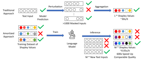
To achieve a better trade-off between efficiency and stability, we propose a simple yet effective amortization method to estimate the explanation scores. Motivated by the observation that different instances might share a similar set of important words (e.g., in sentiment classification, emotional words are strong label indicators (Taboada et al., 2011)), an amortized model can leverage similar interpretation patterns across instances when predicting the explanation scores. Specifically, we amortize the cost of computing explanation scores by precomputing them on a set of training examples and train an amortized model to predict the explanation scores given the input. At inference time, our amortized model directly outputs explanation scores for new instances. Although we need to collect a training set for every model we wish to interpret, our experiments show that with as few as 5000 training instances, the amortized model achieves high estimation accuracy. We show our proposed amortized model in Figure 2.
The experimental results demonstrate the efficiency and effectiveness of our approach. First, our model reduces the computation time from about 3.47s per instance to less than 50ms,111On Yelp-Polarity dataset and using A100 GPU, we compare with typical KS running with 200 samples. which is 60 times faster than the baseline methods. Second, our model is robust to randomness in training (e.g., random initialization, random seeds used for generating reference explanation scores in the training dataset), and produces stable estimations over different random seeds. Third, we show that the amortized model can be used along with SVS to perform local adaption, i.e., adapting to specific instances at inference time, thus further improving performance if more computation is available (6.3). Finally, we evaluate our model from the functionality perspective (Doshi-Velez and Kim, 2017; Ye and Durrett, 2022) by examining the quality of the explanation in downstream tasks. We perform case studies on feature selection and domain calibration using the estimated explanation scores, and show that our method outperforms the computationally expensive KS method.
2 Related Works
Post-Hoc Local Explanation Methods Post-hoc local explanations are proposed to understand the prediction process of neural models (Simonyan et al., 2014; Ribeiro et al., 2016; Lundberg and Lee, 2017; Shrikumar et al., 2017). They work by assigning an explanation score to each feature (e.g., a token) in an instance (“local”) to indicate its contribution to the model prediction. In this paper, we focus on studying KernelSHAP (KS) (Lundberg and Lee, 2017), an additive feature attribution method that estimates the Shapley Value (Shapley, 1953) for each feature.
There are other interpretability methods in NLP. For example, gradient-based methods (Simonyan et al., 2014; Li et al., 2016), which use the gradient w.r.t. each input dimension as a measure for its saliency. Reference-based methods (Shrikumar et al., 2017; Sundararajan et al., 2017) consider the model output difference between the original input and reference input (e.g., zero embedding vectors).
Shapley Values Estimation Shapley Values are concepts from game theory to attribute total contribution to individual features. However, in practice estimating Shapley values requires prohibitively high cost for computation, especially when explaining the prediction on long documents in NLP. KS works as an efficient way to approximate Shapley Values. Previous work on estimating Shapley Values mainly focuses on accelerating the sampling process (Jethani et al., 2021; Covert and Lee, 2021; Parvez and Chang, 2021; Mitchell et al., 2022) or removing redundant features (Aas et al., 2021; Covert et al., 2021). In this work, we propose a new method to combat this challenge by training an amortized model.
Robustness of Local Explanation Methods Despite being widely adopted, there has been a long discussion on the actual quality of explanation methods. Recently, people have found that explanation methods can assign substantially different attributions to similar inputs (Alvarez-Melis and Jaakkola, 2018; Ghorbani et al., 2019; Kindermans et al., 2019; Yeh et al., 2019; Slack et al., 2021; Yin et al., 2022), i.e., they are not robust enough, which adds to the concerns about how faithful these explanations are (Doshi-Velez and Kim, 2017; Adebayo et al., 2018; Jacovi and Goldberg, 2020). In addition to previous work focusing on robustness against input perturbations, we demonstrate that even just changing the random seeds can cause the estimated Shapley Values to be weakly-correlated with each other, unless a large number of perturbation samples are used (which incurs high computational cost).
Amortized Explanation Methods Our method is similar to recent works on amortized explanation models including CXPlain (Schwab and Karlen, 2019) and FastSHAP (Jethani et al., 2021)), where they also aim to improve the computational efficiency of explanation methods. The key differences are: 1) We do not make causal assumptions between input features and model outputs; and 2) we focus on text domains, where each feature is a discrete token (typical optimization methods for continuous variables do not directly apply).
3 Background
In this section, we briefly review the basics of Shapley Values, focusing on its application to the text classification task.
Local explanation of black-box text classification models. In text classification tasks, inputs are usually sequences of discrete tokens . Here is the length of and may vary across examples; is the -th token of . The classification model takes the input and predict the label as . Local explanation methods treat each data instance independently and compute an explanation score , representing the contribution of to the label . Usually, we care about the explanation scores when .
Shapley Values (SV) are concepts from game theory originally developed to assign credits in cooperative games (Shapley, 1953; Strumbelj and Kononenko, 2010; Lundberg and Lee, 2017; Covert et al., 2021). Let be a masking of the input and define as the perturbed input that consists of unmasked tokens (where the corresponding mask has a value of 1). In this paper, we follow the common practice (Ye et al., 2021; Ye and Durrett, 2022; Yin et al., 2022) to replace masked tokens with [PAD] in the input before sending it to the classifier. Let represent the number of non-zero terms in . Shapley Values (Shapley, 1953) are computed by:
| (1) |
Intuitively, computes the marginal contributions of each token to the model prediction.
Computing SV is known to be NP-hard (Deng and Papadimitriou, 1994). In practice, we estimate Shapley Values approximately for efficiency. Shapley Values Sampling (SVS) (Castro et al., 2009; Strumbelj and Kononenko, 2010) is a widely-used Monte-Carlo estimator of SV:
| (2) |
Here is the sampled ordering and is the non-ordered set of indices for . represents the set of indices ranked lower than in . maps the indices set to a mask such that . is the number of perturbation samples used for computing SVS.
KernelSHAP Although SVS has successfully reduced the exponential time complexity to polynomial, it still requires sampling permutations and needs to do sequential updates following sampled orderings and computing the explanation scores, which is an apparent efficiency bottleneck. Lundberg and Lee (2017) introduce a more efficient estimator, KernelSHAP (KS), which allows better parallelism and computing explanation scores for all tokens at once using linear regression. That is achieved by showing that computing SV is equivalent to solving the following optimization problem:
| (3) | |||
where is the one-hot vector corresponding to the mask222Note, is the -th mask sample while is the -th dimension of the mask sample . sampled from the Shapley Kernel . is again the number of perturbation samples. We will use “SVS-” and “KS-” in the rest of the paper to indicate the sample size for SVS and KS. In practice, the specific perturbation samples depend on the random seed of the sampler, and we will show that the explanation scores are highly sensitive to the random seed under a small sample size.
Note that the larger the number of perturbation samples, the more model evaluations are required for a single instance, which can be computationally expensive for large Transformer models. Therefore, the main performance bottleneck is the number of model evaluations.
4 Stability of Local Explanation
One of the most common applications of SV is feature selection, which selects the most important features by following the order of the explanation scores. People commonly use KS with an affordable number of perturbation samples in practice (the typical numbers of perturbation samples used in the literature are around , , ). However, as we see in Figure 1, the ranking of the scores can be quite sensitive to random seeds when using stochastic estimation of SV. In this section, we investigate this stability issue. We demonstrate stochastic approximation of SV is unstable in text classification tasks under common settings, especially with long texts. In particular, when ranking input tokens based on explanation scores, Spearman’s correlation between rankings across different runs is low.
Measuring ranking stability. Given explanation scores produced by different random seeds using an SV estimator, we want to measure the difference between these scores. Specifically, we are interested in the difference in the rankings of the scores as this is what we use for feature selection. To measure the ranking stability of multiple runs using different random seeds, we compute Spearman’s correlation between any two of them and use the average Spearman’s correlation as the measure of the ranking stability. In addition, we follow Ghorbani et al. (2019) to report Top-K intersections between two rankings, since in many applications only the top features are of explanatory interest. We measure the size of the intersection of Top-K features from two different runs.
| Setting | Spearman | Top-5 Inter. | Top-10 Inter. | MSE | Running Time |
|---|---|---|---|---|---|
| SVS-25 | s/it | ||||
| KS-25 | s/it | ||||
| KS-200 | s/it | ||||
| KS-2000 | s/it | ||||
| KS-8000 | s/it |
| Setting | Spearman | Top-5 Inter. | Top-10 Inter. | MSE | Running Time |
|---|---|---|---|---|---|
| SVS-25 | s/it | ||||
| KS-25 | s/it | ||||
| KS-200 | s/it | ||||
| KS-2000 | s/it | ||||
| KS-8000 | s/it |
Setup. We conduct our experiments on the validation set of the Yelp-Polarity dataset (Zhang et al., 2015) and MNLI dataset (Williams et al., 2018). Yelp-Polarity is a binary sentiment classification task and MNLI is a three-way textual entailment classification task.
We conduct experiments on random samples with balanced labels (we refer to these datasets as “Stability Evaluation Sets” subsequently). Results are averaged over different random seeds.333We take more than 2,000 hours on a single A100 GPU for all experiments in this section. We use the publicly available fine-tuned BERT-base-uncased checkpoints444Yelp-Polarity: https://huggingface.co/textattack/bert-base-uncased-yelp-polarity
MNLI: https://huggingface.co/textattack/bert-base-uncased-MNLI (Morris et al., 2020) as the target models to interpret and use the implementation of Captum (Kokhlikyan et al., 2020) to compute the explanation scores for both KS and SVS.
For each explanation method, we test with the recommended numbers of perturbation samples555For SVS, the recommended number of perturbation samples is in Captum. For KS, to our best knowledge, the typical numbers of perturbation samples used in previous works are . We also include KS- to see how stable KS can be given much longer running time.
used to compute the explanation scores for every instance. For Top-K intersections, we report results with and .
Trade-off between stability and computation cost. The ranking stability results are listed in Table 1 and Table 2 for Yelp-Polarity and MNLI datasets. We observe that using 25 to 200 perturbation samples, the stability of the explanation scores is low (Spearman’s correlation is only 0.16). Sampling more perturbed inputs makes the scores more stable. However, the computational cost explodes at the same time, going from one second to two minutes per instance. To reduce the sensitivity to an acceptable level (i.e., making the Spearman’s correlation between two different runs above , which indicates moderate correlation Akoglu (2018)), we usually need thousands of model evaluations and spend roughly seconds per instance.
Low MSE does not imply stability. Mean Squared Error (MSE) is commonly used to evaluate the distance between two lists of explanation scores. In Table 1, we observe that MSE only weakly correlates with ranking stability (e.g., For Yelp-Polarity, and , so the correlation is not significant). Even when the difference of MSE for different settings is as low as 0.01, the correlation between rankings produced by explanations can still be low. Therefore, from users’ perspectives, low MSEs do not mean the explanations are reliable as they can suggest distinct rankings.
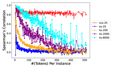
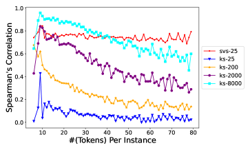
Longer input suffers more from instability. We also plot the Spearman’s correlation decomposed at different input lengths in Figure 3. Here, we observe a clear trend that the ranking stability degrades significantly even at an input length of 20 tokens. The general trend is that the longer the input length is, the worse the ranking stability. The same trend holds across datasets. As many NLP tasks involve sentences longer than 20 tokens (e.g., SST-2 Socher et al. (2013), MNLI Williams et al. (2018)), obtaining stable explanations to analyze NLP models can be quite challenging.
Discussion: why Shapley Values estimation is unstable in text domain? One of the most prominent characteristics of the text domain is that individual tokens/n-grams can have a large impact on the label. Thus they need to be all included in the perturbation samples for an accurate estimate. When the input length grows, the number of n-grams will grow fast. As shown in Section 3, the probability of certain n-grams getting sampled is drastically reduced as each n-gram will be sampled with equivalent probability. Therefore, the observed model output will have a large variance as certain n-grams may not get sampled. A concurrent work Kwon and Zou (2022) presented a related theoretical analysis on why the uniform sampling setting in SV computation can lead to suboptimal attribution.
5 Amortized Inference for Shapley Values
Motivated by the above observation, we propose to train an amortized model to predict the explanation scores given an input without any model evaluation on perturbation samples. The inference cost is thus amortized by training on a set of pre-computed reliable explanation scores.
We build an amortized explanation model for text classification in two stages. In the first stage, we construct a training set for the amortized model. We compute reliable explanation scores as the reference scores for training using the existing SV estimator. As shown in Section 4, SVS-25 is the most stable SV estimator and we use it to obtain reference scores. In the second stage, we train a BERT-based amortized model that takes the text as input and outputs the explanation scores using MSE loss.
Specifically, given input tokens , we use a pretrained language model to encode words into -dim embeddings . Then, we use a linear layer to transform each to the predicted explanation score . To train the model, we use MSE loss to fit to the pre-computed reference scores over the training set . This is an amortized model in the sense that there are no individual sampling and model queries for each test example as in SVS and KS. When a new sample comes in, the amortized model makes a single inference on the input tokens to predict their explanation scores.
5.1 Better Fit via Local Adaption
By amortization, our model can learn to capture the shared feature attribution patterns across data to achieve a good efficiency-stability trade-off. We further show that the explanations generated by our amortized model can be used to initialize the explanation scores of SVS. This way, the evaluation of SVS can be significantly sped up compared with using random initialization. On the other hand, applying SVS upon amortized method improves the latter’s performance as some important tokens might not be captured by the amortized method but can be identified by SVS through additional sampling (e.g., low-frequency tokens). The detailed algorithm is shown in Algorithm 1. Note that here we can recover the original SVS computation (Strumbelj and Kononenko, 2010) by replacing to be . is the amortized model trained using MSE as explained earlier.
6 Experiments
In this section, we present experiments to demonstrate the properties of the proposed approach in terms of accuracy against reference scores (6.1) and sensitivity to training-time randomness (6.2). We also show that we achieve a better fit via a local adaption method that combines our approach with SVS (6.3). Then, we evaluate the quality of the explanations generated by our amortized model on two downstream applications (6.5).
Setup. We conduct experiments on the validation set of Yelp-Polarity and MNLI datasets. To generate reference explanation scores, we leverage the Thermostat (Feldhus et al., 2021) dataset, which contains 9,815 pre-computed explanation scores of SVS-25 on MNLI. We also compute explanation scores of SVS-25 for 25,000 instances on Yelp-Polarity. We use BERT-base-uncased (Devlin et al., 2019) for . For dataset preprocessing and other experiment details, we refer readers to Appendix C.
To our best knowledge, FastSHAP (Jethani et al., 2021) is the most relevant work to us that also takes an amortization approach to estimate SV on tabular or image data. We adapt it to explain the text classifier and use it as a baseline to compare with our approach. We find it non-trivial to adapt FastSHAP to the text domain. As pre-trained language models occupy a large amount of GPU memory, we can only use a small batch size with limited perturbation samples (i.e., perturbation samples per instance). This is equivalent to approximate KS-32 and the corresponding reference explanation scores computed by FastSHAP are unstable. More details can be found in Appendix A.
| Method | MNLI | Yelp-Polarity | ||
| Spearman | MSE | Spearman | MSE | |
| SVS-25 | 0.75 | 1.90e-2 | 0.84 | 6.64e-3 |
| KS-25 | 0.17 | 9.95e-2 | 0.12 | 4.34e-2 |
| KS-200 | 0.35 | 7.73e-2 | 0.24 | 5.77e-2 |
| KS-2000 | 0.60 | 2.54e-2 | 0.51 | 1.86e-2 |
| KS-8000 | 0.74 | 1.25e-2 | 0.70 | 6.25e-3 |
| FastSHAP | 0.23 | 1.90e-1 | 0.18 | 7.91e-3 |
| Our Amortized Model | 0.42 | 9.59e-3 | 0.61 | 4.46e-6 |
6.1 Shapley Values Approximation
To examine how well our model fits the pre-computed SV (SVS-25), we compute both Spearman’s correlation and MSE over the test set. As it is intractable to compute exact Shapley Values for ground truth, we use SVS-25 as a proxy. We also include different settings for KS results over the same test set. KS is also an approximation to permutation-based SV computation (Lundberg and Lee, 2017). Table 3 shows the correlation and MSE of aforementioned methods against SVS-25.
First, we find that despite the simplicity of our amortized model, the proposed amortized models achieve a high correlation with the reference scores () on Yelp-Polarity. The correlation between outputs from the amortized models and references is moderate () on MNLI when data size is limited. During inference time, our amortized models output explanation scores for each instance within milliseconds, which is about - times faster than KS-200 and - times faster than KS-2000 on Yelp-Polarity and MNLI. Although the approximation results are not as good as KS-2000/8000 (which requires far more model evaluations), our approach achieves reasonably good results with orders of magnitude less compute.
We also find that the amortized model achieves the best MSE score among all approximation methods. Note that the two metrics, Spearman’s correlation and MSE, do not convey the same information. MSE measures how well the reference explanation scores are fitted while Spearman’s correlation reflects how well the ranking information is learned. We advocate for reporting both metrics.
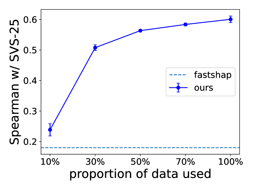
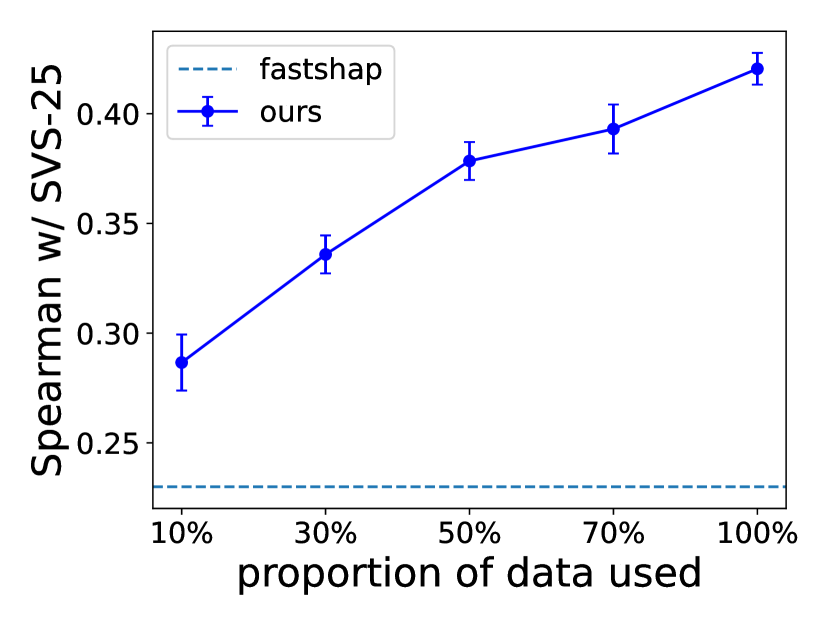
Cost of training the amortized models To produce the training set, we need to pre-compute the explanation scores on a set of data. Although this is a one time cost (for each model), one might wonder how time consuming this step is as we need to run the standard sample-based estimation. As the learning curve shows in Figure 4, we observe that the model achieves good performance with about ( on Yelp-Polarity) instances. Additionally, in Section 6.4, we show this one-time training will result in a model transferable to other domains, so we may not need to train a new amortized model for each new domain.
| Training Data Proportion | Spearman (MNLI) | Spearman (Yelp-Polarity) |
| 10% | 0.45 | 0.40 |
| 30% | 0.57 | 0.65 |
| 50% | 0.65 | 0.71 |
| 70% | 0.65 | 0.72 |
| 100% | 0.77 | 0.76 |
6.2 Sensitivity Analysis
Given a trained amortized model, there is no randomness when generating explanation scores. However, there is still some randomness in the training process, including the training data, the random initialization of the output layer and randomness during update such as dropout. Therefore, similar to Section 4, we study the sensitivity of the amortized model. Table 4 shows the results with different training data and random seeds. We observe that: 1) when using the same data (100%), random initialization does not affect the outputs of amortized models – the correlation between different runs is high (i.e., on MNLI and on Yelp-Polarity). 2) With more training samples, the model is more stable.
| Method | MNLI | Yelp-Polarity |
| Spearman | Spearman | |
| SVS-2 | 0.41 | 0.52 |
| SVS-3 | 0.47 | 0.60 |
| SVS-5 | 0.55 | 0.69 |
| SVS-25 | 0.75 | 0.84 |
| Our Amortized Model | 0.42 | 0.61 |
| Our Amortized Model (Adapt-2) | 0.47 | 0.64 |
| Our Amortized Model (Adapt-3) | 0.53 | 0.69 |
| Our Amortized Model (Adapt-5) | 0.57 | 0.71 |
6.3 Local Adaption
The experiment results for Local Adaption (Section 5.1) are shown in Table 5. Here we can see that: 1) by doing local adaption, we can further improve the approximation results using our amortized model, 2) by using our amortized model as initialization, we can improve the sample efficiency of SVS significantly (by comparing the performance of SVS-X and Adapt-X). These findings hold across datasets.
6.4 Domain Transferability
To see how well our model performs on out-of-domain data, we train a classification model and its amortized explanation model on Yelp-Polarity and then explain its performance on SST-2 Socher et al. (2013) validation set. Both tasks are two-way sentiment classification and have significant domain differences.
Our amortized model achieves a Spearman’s correlation of approximately 0.50 with ground truth SV (SVS-25) while only requiring 0.017s per instance. In comparison, KS-100 achieves a lower Spearman’s correlation of 0.46 with the ground truth and takes 1.6s per instance; KS-200 performs slightly better in Spearman’s correlation but requires significantly more time. Thus, our amortized model is more than 90 times faster and more correlated with ground truth Shapley Values. This shows that, once trained, our amortized model can provide efficient and stable estimations of SV even for out-of-domain data.
In practice, we do not recommend directly explaining model predictions on out-of-domain data without verification, because it may be misaligned with user expectations for explanations, and the out-of-domain explanations may not be reliable Hase et al. (2021); Denain and Steinhardt (2022). More exploration on this direction is required but is orthogonal to this work.
6.5 Evaluating the Quality of Explanation
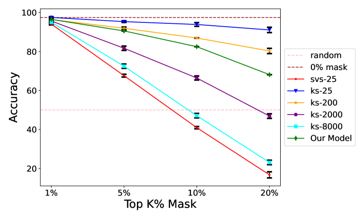
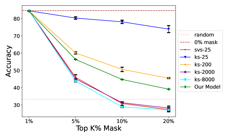
Feature Selection. The first case study is feature selection, which is a straightforward application of local explanation scores. The goal is to find decision-critical features via removing input features gradually according to the rank given by the explanation methods. Following previous work Zaidan et al. (2007); Jain and Wallace (2019); DeYoung et al. (2020), we measure faithfulness by changes in the model output after masking tokens identified as important by the explanation method. The more faithful the explanation method is to the target model, the more performance drop will be incurred by masking important tokens.
We gradually mask Top- tokens () and compute the accuracy over corrupted results using the stability evaluation sets for MNLI and Yelp-Polarity datasets as mentioned in Section 4. As the results show in Figure 5, the amortized model is more faithful than KS-200 but underperforms KS-2000/8000 and SVS-25. However, the amortized model is more efficient than these methods. So amortized model achieves a better efficiency-faithfulness trade-off.
Explanation for Model Calibration. Recent work suggests that good explanations should be informative enough to help users to predict model behavior (Doshi-Velez and Kim, 2017; Chandrasekaran et al., 2018; Hase and Bansal, 2020; Ye et al., 2021). Ye and Durrett (2022) propose to combine the local explanation with pre-defined feature templates (e.g., aggregating explanation scores for overlapping words / POS Tags in NLI as features) to calibrate an existing model to new domains. The rationale behind this is that, if the local explanation truly connects to human-understandable model behavior, then following the same way how humans transfer knowledge to new domains, the explanations guided by human heuristics (in the form of feature templates) should help calibrate the model to new domains. Inspired by this, we conduct a study using the same calibrator architecture but plugging in different local explanation scores.
We follow Ye and Durrett (2022) to calibrate a fine-tuned MNLI model666https://huggingface.co/textattack/bert-base-uncased-MNLI to MRPC. The experiment results are shown in Table 6. In the table, “BOW” means the baseline that uses constant explanation scores when building the features for the calibration model. Compared with the explanation provided by KS-2000, the explanation given by the amortized model achieves better accuracy, suggesting that the amortized model learns robust explanation scores that can be generalized to out-of-domain data in downstream applications.777See Section 6.4 for a domain transfer experiment that directly compares to SVS-25 and w/o calibration.
| Model | Acc | |
|---|---|---|
| BOW | 67.3 | |
| ShapCal (KS-2000) | 67.4 | |
| ShapCal (Amortized) | 68.0 |
7 Conclusion
In this paper, we empirically demonstrated that it is challenging to obtain stable explanation scores on long text inputs. Inspired by the fact that different instances can share similarly important features, we proposed to efficiently estimate the explanation scores through an amortized model trained to fit pre-computed reference explanation scores.
In the future, we plan to explore model architecture and training loss for developing effective amortized models. In particular, we may incorporate sorting-based loss to learn the ranking order of features. Additionally, we could investigate the transferability of the amortized model across different domains, as well as exploring other SHAP-based methods instead of the time-consuming SVS-25 in the data collection process to improve efficiency further.
Limitations
In this paper, we mainly focus on developing an amortized model to efficiently achieve a reliable estimation of SV. Though not experimented with in the paper, our method can be widely applied to other black-box post-hoc explanation methods including LIME Ribeiro et al. (2016). Also, due to the limited budget, we only run experiments on BERT-based models. However, as we do not make any assumption for the model as other black-box explanation methods, our amortized model can be easily applied to other large language models. We only need to collect the model output and our model can be trained offline with just thousands of examples as we show in our method and experiments.
Comparison and Training with Exact Shapley Values Computing exact SV is computationally prohibitive for large language models (LLMs) on lengthy text inputs, as it necessitates the evaluation of LLMs on an exponential (in sequence length) number of perturbation samples per instance. As a result, we resort to using SVS-25, which serves as a reliable approximation, for training our amortized models.
Acknowledgements
We want to thank Xi Ye and Prof. Greg Durrett for their help regarding their previous work and implementation on using SV for calibration (Section 6.5). We thank the generous support from AWS AI on computational resources and external collaborations. We further thank Prof. Chenhao Tan for the high-level idea discussion on explainability stability issues at an early stage of this paper, and thank Prof. Yongchan Kwon and Prof. James Zou for their in-depth theoretical analysis of suboptimality of uniform sampling of computing SV. We thank all anonymous reviewers and chairs at ACL’23 and ICLR’23 for their insightful and helpful comments. Yin and Chang are supported in part by a CISCO grant and a Sloan Fellowship. HH is supported in part by a Cisco grant and Samsung Research (under the project Next Generation Deep Learning: From Pattern Recognition to AI).
References
- Aas et al. (2021) Kjersti Aas, Martin Jullum, and Anders Løland. 2021. Explaining individual predictions when features are dependent: More accurate approximations to shapley values. Artificial Intelligence, 298:103502.
- Adebayo et al. (2018) Julius Adebayo, Justin Gilmer, Michael Muelly, Ian J. Goodfellow, Moritz Hardt, and Been Kim. 2018. Sanity checks for saliency maps. In Advances in Neural Information Processing Systems 31: Annual Conference on Neural Information Processing Systems 2018, NeurIPS 2018, December 3-8, 2018, Montréal, Canada, pages 9525–9536.
- Akoglu (2018) Haldun Akoglu. 2018. User’s guide to correlation coefficients. Turkish journal of emergency medicine, 18(3):91–93.
- Alvarez-Melis and Jaakkola (2018) David Alvarez-Melis and Tommi S Jaakkola. 2018. On the robustness of interpretability methods. Proceedings of the ICML Workshop on Human Interpretability in Machine Learning (WHI 2018).
- Castro et al. (2009) Javier Castro, Daniel Gómez, and Juan Tejada. 2009. Polynomial calculation of the shapley value based on sampling. Computers & Operations Research, 36(5):1726–1730.
- Chandrasekaran et al. (2018) Arjun Chandrasekaran, Viraj Prabhu, Deshraj Yadav, Prithvijit Chattopadhyay, and Devi Parikh. 2018. Do explanations make VQA models more predictable to a human? In Proceedings of the 2018 Conference on Empirical Methods in Natural Language Processing, pages 1036–1042, Brussels, Belgium. Association for Computational Linguistics.
- Covert and Lee (2021) Ian Covert and Su-In Lee. 2021. Improving kernelshap: Practical shapley value estimation using linear regression. In The 24th International Conference on Artificial Intelligence and Statistics, AISTATS 2021, April 13-15, 2021, Virtual Event, volume 130 of Proceedings of Machine Learning Research, pages 3457–3465. PMLR.
- Covert et al. (2021) Ian Covert, Scott M Lundberg, and Su-In Lee. 2021. Explaining by removing: A unified framework for model explanation. Journal of Machine Learning Research, 22:209–1.
- Denain and Steinhardt (2022) Jean-Stanislas Denain and Jacob Steinhardt. 2022. Auditing visualizations: Transparency methods struggle to detect anomalous behavior. ArXiv preprint, abs/2206.13498.
- Deng and Papadimitriou (1994) Xiaotie Deng and Christos H Papadimitriou. 1994. On the complexity of cooperative solution concepts. Mathematics of operations research, 19(2):257–266.
- Devlin et al. (2019) Jacob Devlin, Ming-Wei Chang, Kenton Lee, and Kristina Toutanova. 2019. BERT: Pre-training of deep bidirectional transformers for language understanding. In Proceedings of the 2019 Conference of the North American Chapter of the Association for Computational Linguistics: Human Language Technologies, Volume 1 (Long and Short Papers), pages 4171–4186, Minneapolis, Minnesota. Association for Computational Linguistics.
- DeYoung et al. (2020) Jay DeYoung, Sarthak Jain, Nazneen Fatema Rajani, Eric Lehman, Caiming Xiong, Richard Socher, and Byron C. Wallace. 2020. ERASER: A benchmark to evaluate rationalized NLP models. In Proceedings of the 58th Annual Meeting of the Association for Computational Linguistics, pages 4443–4458, Online. Association for Computational Linguistics.
- Doshi-Velez and Kim (2017) Finale Doshi-Velez and Been Kim. 2017. Towards a rigorous science of interpretable machine learning. ArXiv preprint, abs/1702.08608.
- Feldhus et al. (2021) Nils Feldhus, Robert Schwarzenberg, and Sebastian Möller. 2021. Thermostat: A large collection of NLP model explanations and analysis tools. In Proceedings of the 2021 Conference on Empirical Methods in Natural Language Processing: System Demonstrations, pages 87–95, Online and Punta Cana, Dominican Republic. Association for Computational Linguistics.
- Ghorbani et al. (2019) Amirata Ghorbani, Abubakar Abid, and James Y. Zou. 2019. Interpretation of neural networks is fragile. In The Thirty-Third AAAI Conference on Artificial Intelligence, AAAI 2019, The Thirty-First Innovative Applications of Artificial Intelligence Conference, IAAI 2019, The Ninth AAAI Symposium on Educational Advances in Artificial Intelligence, EAAI 2019, Honolulu, Hawaii, USA, January 27 - February 1, 2019, pages 3681–3688. AAAI Press.
- Hase and Bansal (2020) Peter Hase and Mohit Bansal. 2020. Evaluating explainable AI: Which algorithmic explanations help users predict model behavior? In Proceedings of the 58th Annual Meeting of the Association for Computational Linguistics, pages 5540–5552, Online. Association for Computational Linguistics.
- Hase et al. (2021) Peter Hase, Harry Xie, and Mohit Bansal. 2021. The out-of-distribution problem in explainability and search methods for feature importance explanations. Advances in Neural Information Processing Systems, 34:3650–3666.
- Jacovi and Goldberg (2020) Alon Jacovi and Yoav Goldberg. 2020. Towards faithfully interpretable NLP systems: How should we define and evaluate faithfulness? In Proceedings of the 58th Annual Meeting of the Association for Computational Linguistics, pages 4198–4205, Online. Association for Computational Linguistics.
- Jain and Wallace (2019) Sarthak Jain and Byron C. Wallace. 2019. Attention is not Explanation. In Proceedings of the 2019 Conference of the North American Chapter of the Association for Computational Linguistics: Human Language Technologies, Volume 1 (Long and Short Papers), pages 3543–3556, Minneapolis, Minnesota. Association for Computational Linguistics.
- Jethani et al. (2021) Neil Jethani, Mukund Sudarshan, Ian Connick Covert, Su-In Lee, and Rajesh Ranganath. 2021. Fastshap: Real-time shapley value estimation. In International Conference on Learning Representations.
- Kindermans et al. (2019) Pieter-Jan Kindermans, Sara Hooker, Julius Adebayo, Maximilian Alber, Kristof T Schütt, Sven Dähne, Dumitru Erhan, and Been Kim. 2019. The (un) reliability of saliency methods. In Explainable AI: Interpreting, Explaining and Visualizing Deep Learning, pages 267–280. Springer.
- Kingma and Ba (2015) Diederik P. Kingma and Jimmy Ba. 2015. Adam: A method for stochastic optimization. In 3rd International Conference on Learning Representations, ICLR 2015, San Diego, CA, USA, May 7-9, 2015, Conference Track Proceedings.
- Kokhlikyan et al. (2020) Narine Kokhlikyan, Vivek Miglani, Miguel Martin, Edward Wang, Bilal Alsallakh, Jonathan Reynolds, Alexander Melnikov, Natalia Kliushkina, Carlos Araya, Siqi Yan, et al. 2020. Captum: A unified and generic model interpretability library for pytorch. ArXiv preprint, abs/2009.07896.
- Kwon and Zou (2022) Yongchan Kwon and James Zou. 2022. Weightedshap: analyzing and improving shapley based feature attributions. Advances in Neural Information Processing Systems.
- Li et al. (2016) Jiwei Li, Xinlei Chen, Eduard Hovy, and Dan Jurafsky. 2016. Visualizing and understanding neural models in NLP. In Proceedings of the 2016 Conference of the North American Chapter of the Association for Computational Linguistics: Human Language Technologies, pages 681–691, San Diego, California. Association for Computational Linguistics.
- Lundberg and Lee (2017) Scott M. Lundberg and Su-In Lee. 2017. A unified approach to interpreting model predictions. In Advances in Neural Information Processing Systems 30: Annual Conference on Neural Information Processing Systems 2017, December 4-9, 2017, Long Beach, CA, USA, pages 4765–4774.
- Mitchell et al. (2022) Rory Mitchell, Joshua Cooper, Eibe Frank, and Geoffrey Holmes. 2022. Sampling permutations for shapley value estimation. Journal of Machine Learning Research, 23(43):1–46.
- Morris et al. (2020) John Morris, Eli Lifland, Jin Yong Yoo, Jake Grigsby, Di Jin, and Yanjun Qi. 2020. TextAttack: A framework for adversarial attacks, data augmentation, and adversarial training in NLP. In Proceedings of the 2020 Conference on Empirical Methods in Natural Language Processing: System Demonstrations, pages 119–126, Online. Association for Computational Linguistics.
- Parvez and Chang (2021) Md Rizwan Parvez and Kai-Wei Chang. 2021. Evaluating the values of sources in transfer learning. In Proceedings of the 2021 Conference of the North American Chapter of the Association for Computational Linguistics: Human Language Technologies, pages 5084–5116, Online. Association for Computational Linguistics.
- Ribeiro et al. (2016) Marco Túlio Ribeiro, Sameer Singh, and Carlos Guestrin. 2016. "why should I trust you?": Explaining the predictions of any classifier. In Proceedings of the 22nd ACM SIGKDD International Conference on Knowledge Discovery and Data Mining, San Francisco, CA, USA, August 13-17, 2016, pages 1135–1144. ACM.
- Schwab and Karlen (2019) Patrick Schwab and Walter Karlen. 2019. Cxplain: Causal explanations for model interpretation under uncertainty. In Advances in Neural Information Processing Systems 32: Annual Conference on Neural Information Processing Systems 2019, NeurIPS 2019, December 8-14, 2019, Vancouver, BC, Canada, pages 10220–10230.
- Shapley (1953) Lloyd S Shapley. 1953. A value for n-person games. In Harold W. Kuhn and Albert W. Tucker, editors, Contributions to the Theory of Games II, pages 307–317. Princeton University Press, Princeton.
- Shrikumar et al. (2017) Avanti Shrikumar, Peyton Greenside, and Anshul Kundaje. 2017. Learning important features through propagating activation differences. In Proceedings of the 34th International Conference on Machine Learning, ICML 2017, Sydney, NSW, Australia, 6-11 August 2017, volume 70 of Proceedings of Machine Learning Research, pages 3145–3153. PMLR.
- Simonyan et al. (2014) Karen Simonyan, Andrea Vedaldi, and Andrew Zisserman. 2014. Deep inside convolutional networks: Visualising image classification models and saliency maps. CoRR, abs/1312.6034.
- Slack et al. (2021) Dylan Slack, Anna Hilgard, Sameer Singh, and Himabindu Lakkaraju. 2021. Reliable post hoc explanations: Modeling uncertainty in explainability. NeurIPS, 34:9391–9404.
- Socher et al. (2013) Richard Socher, Alex Perelygin, Jean Wu, Jason Chuang, Christopher D. Manning, Andrew Ng, and Christopher Potts. 2013. Recursive deep models for semantic compositionality over a sentiment treebank. In Proceedings of the 2013 Conference on Empirical Methods in Natural Language Processing, pages 1631–1642, Seattle, Washington, USA. Association for Computational Linguistics.
- Strumbelj and Kononenko (2010) Erik Strumbelj and Igor Kononenko. 2010. An efficient explanation of individual classifications using game theory. The Journal of Machine Learning Research, 11:1–18.
- Sundararajan et al. (2017) Mukund Sundararajan, Ankur Taly, and Qiqi Yan. 2017. Axiomatic attribution for deep networks. In Proceedings of the 34th International Conference on Machine Learning, ICML 2017, Sydney, NSW, Australia, 6-11 August 2017, volume 70 of Proceedings of Machine Learning Research, pages 3319–3328. PMLR.
- Taboada et al. (2011) Maite Taboada, Julian Brooke, Milan Tofiloski, Kimberly Voll, and Manfred Stede. 2011. Lexicon-based methods for sentiment analysis. Computational Linguistics, 37(2):267–307.
- Williams et al. (2018) Adina Williams, Nikita Nangia, and Samuel Bowman. 2018. A broad-coverage challenge corpus for sentence understanding through inference. In Proceedings of the 2018 Conference of the North American Chapter of the Association for Computational Linguistics: Human Language Technologies, Volume 1 (Long Papers), pages 1112–1122, New Orleans, Louisiana. Association for Computational Linguistics.
- Ye and Durrett (2022) Xi Ye and Greg Durrett. 2022. Can explanations be useful for calibrating black box models? In Proceedings of the 60th Annual Meeting of the Association for Computational Linguistics (Volume 1: Long Papers), pages 6199–6212, Dublin, Ireland. Association for Computational Linguistics.
- Ye et al. (2021) Xi Ye, Rohan Nair, and Greg Durrett. 2021. Connecting attributions and QA model behavior on realistic counterfactuals. In Proceedings of the 2021 Conference on Empirical Methods in Natural Language Processing, pages 5496–5512, Online and Punta Cana, Dominican Republic. Association for Computational Linguistics.
- Yeh et al. (2019) Chih-Kuan Yeh, Cheng-Yu Hsieh, Arun Sai Suggala, David I. Inouye, and Pradeep Ravikumar. 2019. On the (in)fidelity and sensitivity of explanations. In Advances in Neural Information Processing Systems 32: Annual Conference on Neural Information Processing Systems 2019, NeurIPS 2019, December 8-14, 2019, Vancouver, BC, Canada, pages 10965–10976.
- Yin et al. (2022) Fan Yin, Zhouxing Shi, Cho-Jui Hsieh, and Kai-Wei Chang. 2022. On the sensitivity and stability of model interpretations in NLP. In Proceedings of the 60th Annual Meeting of the Association for Computational Linguistics (Volume 1: Long Papers), pages 2631–2647, Dublin, Ireland. Association for Computational Linguistics.
- Zaidan et al. (2007) Omar Zaidan, Jason Eisner, and Christine Piatko. 2007. Using “annotator rationales” to improve machine learning for text categorization. In Human Language Technologies 2007: The Conference of the North American Chapter of the Association for Computational Linguistics; Proceedings of the Main Conference, pages 260–267, Rochester, New York. Association for Computational Linguistics.
- Zhang et al. (2015) Xiang Zhang, Junbo Jake Zhao, and Yann LeCun. 2015. Character-level convolutional networks for text classification. In Advances in Neural Information Processing Systems 28: Annual Conference on Neural Information Processing Systems 2015, December 7-12, 2015, Montreal, Quebec, Canada, pages 649–657.
Appendix A Adaption for FastSHAP Baseline
As we mentioned in Section 6, we build our amortized models upon a pre-trained encoder BERT (Devlin et al., 2019). However, using the pre-trained encoder significantly increases the memory footprint when running FastSHAP. In particular, we have to host two language models on GPUs, one for the amortized model and the other one for the target model. Therefore, we can only adopt the batch size equal to 1 and perturbation samples per instance. Following the proof in FastSHAP, this is equivalent to teaching the amortized model to approximate KS-32, which is an unreliable interpretation method (See Section 6.2).
In experiments, we find that the optimization of FastSHAP is unstable. After an extensive hyper-parameter search, we set the learning rate to 1e-6 and increased the number of epochs to . However, this requires us to train the model on a single A100 GPU for 3 days to wait for FastSHAP to converge.
Appendix B Scientific Artifacts License
For the datasets used in this paper, MNLI Williams et al. (2018) is released under ONAC’s license. Yelp-Polarity Zhang et al. (2015) and SST-2 Socher et al. (2013) datasets does not provide detailed licenses.
For model checkpoints used in this paper, they all come from textattack project Morris et al. (2020) and they are open-sourced under MIT license.
Appendix C Training Details
In this section, we introduce our dataset preprocessing, hyperparameter settings and how we train the models.
For both MNLI and Yelp-Polarity datasets, we split them into 8:1:1 for training, validation, and test sets.
The hyperparameters of amortized models are tuned on the validation set. We use Adam (Kingma and Ba, 2015) optimizer with a learning rate of 5e-5, train the model for at most 10 epochs and do early stopping to select best model checkpoints.