Hardness and fracture toughness models by symbolic regression

Abstract

Superhard materials with good fracture toughness have found wide industrial applications, which necessitates the development of accurate hardness and fracture toughness models for efficient materials design. Although several macroscopic models have been proposed, they are mostly semiempirical based on prior knowledge or assumptions, and obtained by fitting limited experimental data. Here, through an unbiased and explanatory symbolic regression technique, we built a macroscopic hardness model and fracture toughness model, which only require shear and bulk moduli as inputs. The developed hardness model was trained on an extended dataset, which not only includes cubic systems, but also contains non-cubic systems with anisotropic elastic properties. The obtained models turned out to be simple, accurate, and transferable. Moreover, we assessed the performance of three popular deep learning models for predicting bulk and shear moduli, and found that the crystal graph convolutional neural network and crystal explainable property predictor perform almost equally well, both better than the atomistic line graph neural network. By combining the machine-learned bulk and shear moduli with the hardness and fracture toughness prediction models, potential superhard materials with good fracture toughness can be efficiently screened out through high-throughput calculations.

I Overview of hardness and fracture toughness models

I.1 Superhard materials

Superhard materials have been widely used in many industrial applications due to their unique mechanical properties. They not only have high hardness (usually greater than 40 GPa) Haines et al. (2001), but also often have high fracture toughness and thermal stability Xu and Tian (2015); Gilman et al. (2006); Ivanovskii (2011); Riedel (1994). The hardest known material is diamond, which has a Vickers hardness in the range of 60$\sim$120 GPa. In addition, novel metastable carbon allotropes with comparable Vickers hardness have been experimentally synthesized Mao et al. (2003) or theoretically predicted Li et al. (2009); Niu et al. (2012a); Avery et al. (2019). Some other potentially hard and superhard materials include borides Cheng et al. (2013); Dong et al. (2018); Zhao et al. (2018); Bykova et al. (2022), carbides Chuvil’deev et al. (2015); Sung and Tai (1997), and nitrides Gao et al. (2020); Ivashchenko et al. (2015). Among these materials, cubic boron nitride achieves a second largest hardness of $\sim$60 GPa Tian et al. (2013); Li et al. (2015). In particular, the superhard materials at the nanoscale have achieved excellent mechanical performances Zhao et al. (2016); Hovsepian (2006). This encourages ongoing exploration of reliable models for accurate prediction of hardness and fracture toughness. This is particularly relevant in the context of data-driven high-throughput screening and predictions Choudhary et al. (2018); Kvashnin et al. (2019); Mazhnik and Oganov (2020); Avery et al. (2019).

I.2 Hardness and hardness prediction models

Hardness has long been used as one of the fundamental mechanical properties of materials since 1772 Cole (1957). However, it is not as well defined as other mechanical properties like strength and plasticity Haines et al. (2001). Macroscopically, the hardness of a material is defined as its ability to resist being scratched or dented by other materials. In experiments, the indentation machine is normally used to measure the hardness. According to the different shapes and properties of the indenters, several flavors of the hardness have been developed, e.g., the Brinell hardness, Rockwell hardness, Knoop hardness, and Vickers hardness. Among them, the Vickers and Knoop hardness are most commonly used in standardized tests for engineering and metallurgy Nix and Gao (1998).

Experimentally, hardness is a highly complex property, as the stress applied depends on many factors such as the crystallographic direction, loading force, and the size of the indenter. The same holds also for theory, because the microscopic understanding of the hardness is far from complete, which makes an accurate prediction of the hardness difficult Sun et al. (2022). Despite of this, many microscopic and macroscopic hardness prediction models have been established, with their profound success in the search and prediction of new superhard materials Li et al. (2010); Tian et al. (2012).

By definition, the hardness of a material is intimately linked to its elastic properties. As early as in 1973, Gilman obtained a linear relationship between the hardness and bulk modulus ($B$) Gilman (1973). Then, in 1998 Teter identified a strong correlation between the hardness and shear modulus $H^{\rm Teter}_{V}=0.151G$ Teter (1998). Subsequent study, however, revealed that the hardness is not simply linear to the bulk modulus or shear modulus Chen et al. (2011a). Since the Pugh’s modulus ratio $k=G/B$ Pugh (1954) is closely related to the brittleness/ductility of the material and underlines the relationship between the plastic and elastic properties of pure polycrystalline metals Niu et al. (2012b); Senkov and Miracle (2021), Chen et al. Chen et al. (2011a) proposed a macroscopic hardness model by incorporating the Pugh’s modulus ratio

$$H^{\rm Chen}_{V}=2(k^{2}G)^{0.585}-3.$$ (1)

The Chen’s model has been well appreciated by the community in predicting the hardness of various crystalline materials Chen et al. (2011b); Zhang et al. (2014, 2017, 2022), because the model is very simple, only requires two input parameters ($G$ and $B$) that can be routinely calculated through first-principles calculations, and more importantly, reproduces the experimental hardness data remarkably well Chen et al. (2011a). Nevertheless, the Chen’s model was obtained by fitting the experimental hardness data combined with semiempirical domain knowledge. The data used in fitting are mostly cubic crystals with isotropic elastic properties, which may pose potential risks to the application of the model to systems with strong anisotropic elastic properties. Besides, Tian et al. Tian et al. (2012) noticed that the Chen’s model may yield unphysical negative values when predicting the materials with small hardness due to the presence of an intercept term ($-3$) in the model. To avoid this, they refitted the experimental data compiled in the Chen’s work and proposed a modified formula without the intercept term $H^{\rm Tian}_{V}=0.92k^{1.137}G^{0.708}$ Tian et al. (2012). As expected, both Chen’s and Tian’s models reproduce well the experimental values that were used for fitting. However, when predicting low-hardness materials (e.g., less than 5 GPa), both formulas tend to overestimate the predictions. Motivated by the Chen’s model, Mazhnik and Oganov rewrote the model in terms of Young’s modulus $E$ and Poisson’s ratio $\nu$ using the homogeneous approximation and established a relationship between the hardness and the effective modulus Mazhnik and Oganov (2019). The effective modulus was obtained by fitting the experimental data using a polynomial rational function Mazhnik and Oganov (2019). Although the polynomial rational function increases the flexibility of the model, the resulting hardness model loses the simplicity. In addition, the data used for fitting were also limited to the dataset collected in the Chen’s work, most of which are cubic systems.

In contrast to the macroscopic hardness models, the microscopic hardness models reply on the information (e.g., bond density, bond length, and bonding type, etc.) that can either be derived directly from the crystal structure or extrapolated from the constituent elements Gao et al. (2003); Guo et al. (2008); Li et al. (2008); Šimůnek (2007); Šimůnek and Vackář (2006); Tian et al. (2012); Dai and Zhou (2016). These include the bond resistance models (Gao model Gao et al. (2003) and Guo model Guo et al. (2008)), electronegativity model (Xue model) Li et al. (2008) and bond strength model (SV model) Šimůnek and Vackář (2006). These microscopic hardness models have been successfully applied to covalent and polar covalent crystals, and in some cases, to ionic crystals Tian et al. (2012). Although the microscopic models have their own merits, they are normally not as simple as those macroscopic models. Furthermore, the microscopic models may suffer from the underlying assumptions and predict incorrect hardness values. A typical example is the so-called T-carbon, a novel hypothetical carbon allotrope Sheng et al. (2011). It has a porous structure with a highly anisotropic distribution of the $sp^{3}$-like C-C bonds, and thus is unlikely to be a superhard material. However, the Gao Gao et al. (2003) and SV Šimůnek and Vackář (2006) microscopic models incorrectly predicted the T-carbon to be a superhard material, with an overestimated hardness of 61.1 GPa and 40.5 GPa, respectively. By contrast, the Chen’s macroscopic model yielded a reasonable value of hardness (5.6 GPa) for the T-carbon Chen et al. (2011b). The success of the macroscopic hardness models benefits from the fact that they do not explicitly reply on those not so well-defined quantities like bond electronegativity or bond strength. It is worth noting that recently Podryabinkin et al. Podryabinkin et al. (2022) developed a method that allows to calculate the nanohardness by atomistic simulations of nanoindentation, benefiting from efficient machine-learning interatomic potentials. Despite being accurate, the method is computationally too demanding to enable high-throughput calculations.

I.3 Fracture toughness and its prediction models

Apart from the hardness, searching for hard materials with good fracture toughness is equally important. This is particularly important for practical applications, since the fracture toughness describes the resistance ability of a material against crack propagation and is often an indication of the amount of stress required to propagate a preexisting flaw. The fracture toughness can be quantitatively described by the stress intensity factor $K$, at which a thin crack in the material starts to grow A.E.Carlsson and Thomson (1998). Similarly to the hardness, a large uncertainty is also present in the experimental fracture toughness data, since the values of the fracture toughness are largely influenced by the experimental details like loadings and underlying fracture propagation mechanism. This necessitates the development of fracture toughness prediction models.

However, unlike the hardness models, relatively less efforts have been devoted to developing fracture toughness prediction models. The critical value of the stress intensity factor under mode I loading Griffith and Taylor (1921) is given by $K_{g}=2\sqrt{\gamma_{s}G/(1-\nu)}$ Thomson (1987), where $\gamma_{s}$ is the surface energy of the material and $\nu$ is the Poisson’s ratio. This was derived by balancing the surface tension ($2\gamma_{s}$) of the opening surfaces at the crack tip and the elastic driving force. In practice, $K_{g}$ is much higher than the actual measured value $K_{IC}$, and thus represents the upper bound of fracture toughness Thomson (1987). Through studying the correlation between the fracture toughness and the elastic properties of materials, Niu et al. Niu et al. (2019) developed a fracture toughness prediction model that works well for covalent and ionic crystals

$$K^{\rm Niu}_{IC}=V_{0}^{1/6}G(B/G)^{1/2},$$ (2)

where $V_{0}$ is the volume of the system. It is evident that $K^{\rm Niu}_{IC}$ is also related to the Pugh’s modulus ratio $k=G/B$. We note in passing that Mazhnik and Oganov Mazhnik and Oganov (2019) rewrote the Niu’s model in terms of Young’s modulus and Poisson’s ratio, and proposed a new fracture toughness model based on the effective modulus, which was again obtained by fitting the experimental fracture toughness data using a polynomial rational function Mazhnik and Oganov (2019).

I.4 Data-driven superhard materials predictions

Due to the rapid increase of computing resources, many large public datasets are available Rajan (2015); Malik (1970). Most of the datasets are based on density functional theory (DFT) calculations, e.g., Automatic Flow of Materials Discovery Library (AFLOWLIB) Curtarolo et al. (2012), Open Quantum Materials Database (OQMD) Kirklin et al. (2015), Materials Project (MP) Jain et al. (2013), and Joint Automated Repository for Various Integrated Simulations (JARVIS) Choudhary et al. (2020). This allows us to efficiently search, predict and design materials with target properties, and explore the underlying patterns through the data-driven machine learning (ML) techniques Choudhary et al. (2022); Morgan and Jacobs (2020); Rao et al. (2022); Morgan and Jacobs (2020); Sparks et al. (2020); Suh et al. (2020); Hart et al. (2021); Saal et al. (2020). The workflow of machine learning in general involves the collection and organization of training datasets, design of material descriptors Isayev et al. (2017); Alizadeh and Mohammadizadeh (2019), model regressions, and model validations and predictions. The successful ML models include random forest (RF) Stanev et al. (2017); Ward et al. (2016), neural networks (NN) Shi et al. (2019); Turán (1994), convolutional neural networks (CNN) Tsymbalov et al. (2021), graph convolutional neural networks (GNN) Chen et al. (2019a); Chen and Ong (2021); Xie and Grossman (2017), etc. In the specific field of superhard materials, Avery et al. Avery et al. (2019) and Mazhnik et al. Mazhnik and Oganov (2020) demonstrated the power of combining the ML-derived bulk and shear moduli and the macroscopic Vickers hardness models in predicting novel superhard materials. Tehrani et al. Tehrani et al. (2018) showed how the elastic moduli predicted by the support vector machine were successfully used to guide the synthesis of superhard materials.

I.5 The contribution of this work

In this work, we attempt at building macroscopic hardness and fracture toughness models through the unbiased symbolic regression technique that does not need to make prior assumptions about the specific function form. The dataset used in the regression extends the previously collected experimental dataset (mostly consisting of cubic systems) and involves systems with anisotropic elastic properties. The resulting hardness and fracture toughness models turn out to be very simple and more accurate as compared to the Chen’s hardness model and Niu’s fracture toughness model. Interestingly, the Pugh’s modulus ratio $k=G/B$, a quantity that is closely related to the brittleness/ductility of the material, is naturally included in the regression models. Moreover, we developed machine learning models for efficient and accurate prediction of bulk and shear moduli, the only two required input quantities for the hardness and fracture toughness models. We compared and validated three popular deep learning algorithms including the convolutional neural network, atomistic line graph neural network, and crystal explainable property predictor. With the bulk and shear moduli feeding to the hardness and fracture toughness regression models, several potential superhard materials with good fracture toughness have been predicted through high-throughput calculations.

II Symbolic regression

Although ML models can be pretty predictable, they often contain thousands of parameters and thus require large datasets. More importantly, the ML models typically lack of interpretability, which prevents them from searching for physical laws or finding a neat formula. By contrast, symbolic regression (SR) is an interpretable machine learning algorithm. As a supervised learning method, SR attempts to discover some hidden mathematical formulas so as to predict target variables by using characteristic variables. It is an effective regression method to search for the optimal form of a given set of functions and parameters, even with limited data Wang et al. (2019); Weng et al. (2020); Stephens (2015). For SR, there is no need to presuppose the specific composition of the functions. Instead, one only needs to provide an expression that contains mathematical modules, such as mathematical operators, state variables, analytic functions, etc. Then, SR explores the combinatorial space using these constituent modules to obtain the most suitable scheme Wang et al. (2019). The most common method of SR is genetic programming, which was developed by Koza Koza (1994) as a concrete implementation of genetic algorithms (GA) Forrest (1993). Inspired by the Darwin’s theory of evolution, GA first proposes a tentative solution to a given problem, and then finds the optimal solution after several iterations through crossover and mutation operations. The solutions in genetic programming use a tree structure with nodes and terminals to represent chromosomes. Figure 1(a) shows a chromosome example of a mathematical function $3.0\times x+9.0$. The tree consists of a set of interior nodes with mathematical operations [$+$ (Add) , $\times$ (Mul)] and terminal nodes with variables ($x$) and constants (3.0, 9.0). In order to obtain the final mathematical expression for each individual solution, a depth-first search is performed for traversing the tree.

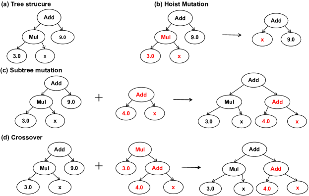
Figure 1: (a) Tree-structure chromosome representation of computer programs in genetic programming. (b) Hoist Mutation. (c) Subtree mutation. (d) Crossover.

The process of symbolic regression starts from a set of randomly generated initial terminal nodes and functions to form trees with different sizes and structures. In this work, the initial terminal nodes were the elastic moduli and randomly generated formula. Then, the ”fitness” of each individual solution was evaluated by comparing the model predictions to the ground truth (i.e., experimental hardness or fracture toughness) in the dataset. The fitness value is an assessment of the accuracy of the resulting formula. The common error measures include mean absolute error (MAE) and root-mean squared error (RMSE). The next generation was then evolved by performing random genetic manipulations [e.g., mutations in Fig. 1(b)-(c) and crossover in Fig. 1(d)] on individual components. The new generation was determined by following the ”survival of the fittest” rule. In this work, the symbolic regression was carried out using gplearn Stephens (2015), a Python library that retains the familiar scikit-learn fit/predict API and works with the existing scikit-learn pipeline and grid search modules Stephens (2015). The hyper-parameters used in this work for gplearn are given in Table 1, and are briefly explained in the following.

For small datasets, a small population size and number of jobs (n-jobs) should be used, which can accelerate the calculation and fast the convergence. For large datasets, such as the extended hardness dataset, the population size and n-jobs need to be appropriately increased in order to obtain a better accuracy. The sum of the four parameters, the probability of crossover (pc), subtree-mutation (ps), hoist-mutation (ph), point-mutation (pp) should be less than or equal to 1. Among them, the ps is an important parameter for avoiding bloat, a phenomenon often encountered in gplearn where the program sizes grow larger and larger but with no significant improvement in fitness. Besides the ps, another important parameter to fight against bloat is the parsimony coefficient: The larger the parsimony coefficient, the shorter the formula.

Table 1: The setup of hyper-parameters used in gplearn for the symbolic regression.

Parameter	Value
population size	2000-8000
n-jobs	3-20
generations	50-200
stopping-criteria	0.01
p-crossover (pc)	0.7(0.6)
p-subtree-mutation (ps)	0.2(0.25)
p-hoist-mutation (ph)	0.05
p-point-mutation (pp)	0.05
p-point-replace (pr)	0.5
parsimony coefficient	0.0001-0.01
metric	mean absolute error
function-set	add, sub, mul, div, sqrt, neg (mul, div, sqrt)

III Results and discussions

III.1 Modeling hardness of polycrystalline materials

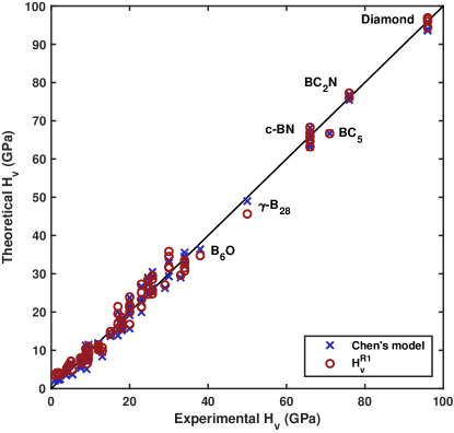
Figure 2: The predicted hardness versus the experimental data using the Chen’s model [Eq. (1)] and the model in Eq. (3). Note that the assessment is performed on the dataset of $T^{A}$ (Table LABEL:tab:TA) on which the two models were obtained.

Let us start from the symbolic regression on the dataset used in the Chen’s work Chen et al. (2011a), taking $B$ and $G$ as input descriptors. We recall that the dataset (referred to as $T^{\rm A}$) contains mostly cubic crystal structures with isotropic elastic properties. The detailed information on $T^{A}$ is given in Table LABEL:tab:TA of the Appendix. The optimal harness model obtained from symbolic regression is expressed as

$$H^{\rm R1}_{V}=0.719kG^{3/4}.$$ (3)

We mean that the model is optimal in the sense of yielding the smallest MAE, but without at the cost of losing the model simplicity. It is surprising to observe that, although $B$ and $G$ are the only two input descriptors, the resulting hardness model naturally incorporates the Pugh’s modulus ratio $k=G/B$. This confirms that the Pugh’s modulus ratio is indeed a good descriptor for the brittleness/ductility of a material.

Figure 2 displayed the predicted hardness using the model in Eq. (3) against the experimental data. For comparison, the hardness predicted using the Chen’s model [Eq. (1)] is also shown. It can be seen that both models reproduce well the experimental data in $T^{A}$ with similar MAEs ($\sim$1.6 GPa) and RMSEs ($\sim$2.0 GPa) (see Table 2). We note that the Tian’s model Tian et al. (2012) obtained by refitting $T^{A}$ exhibits similar performances (see Table 2).

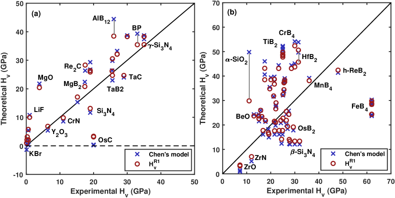
Figure 3: Assessment of the Chen’s model [Eq. (1)] and the model in Eq. (3) for the (a) dataset $T^{B}$ (Table LABEL:tab:TB) and (b) dataset $T^{C}$ (Table LABEL:tab:TC).

Table 2: A summary of MAEs and RMSEs (in GPa) of various hardness models with respect to the experimental data. The dataset used for the assessment is given in parentheses. In the Oganov’s model Mazhnik and Oganov (2019) $H_{V}=0.096\chi(\nu)E$ where $\chi(\nu)=\frac{1-8.5\nu+19.5\nu^{2}}{1-7.5\nu+12.2\nu^{2}-19.6\nu^{3}}$ with $\nu$ and $E$ being the Poisson’s ratio and Young’s modulus, respectively.

	Teter Teter (1998)	Chen Chen et al. (2011a)	Tian Tian et al. (2012)	Oganov Mazhnik and Oganov (2019)	Model $H^{\rm R1}_{V}$ [Eq. (3)]	Model $H^{\rm R2}_{V}$ [Eq. (4)]
	$0.151G$	$2(k^{2}G)^{0.585}-3$	$0.92k^{1.137}G^{0.708}$	$0.096\chi(\nu)E$	$0.719kG^{3/4}$	$0.16k^{1/2}G$
MAE   ($T^{A}$)	3.95	1.58	1.63	4.74	1.62	2.23
RMSE ($T^{A}$)	5.60	2.01	1.97	7.44	2.03	3.05
MAE   ($T^{B}$)	4.79	6.35	5.68	3.76	5.47	4.24
RMSE ($T^{B}$)	6.59	8.62	7.61	4.90	7.35	6.11
MAE   ($T^{C}$)	10.31	14.04	13.14	11.79	12.72	10.90
RMSE ($T^{C}$)	13.26	17.42	16.40	15.78	15.91	14.28
MAE   ($T^{\rm full}$)	6.02	6.27	5.89	5.72	5.70	5.31
RMSE ($T^{\rm full}$)	8.82	10.30	9.65	9.26	9.37	8.56

In order to validate the hardness models, we generated two test datasets. The first one contains the cubic systems that are not included in $T^{A}$ and is referred to as $T^{B}$. The second one includes the non-cubic systems and is called $T^{C}$. The detailed information on $T^{B}$ and $T^{C}$ are provided in Table LABEL:tab:TB and Table LABEL:tab:TC of the Appendix, respectively. The resulting assessment of the models is shown in Fig. 3 with the MAEs and RMSEs being given in Table 2. One can observe that the validation MAEs and RMSEs of the two models on $T^{B}$ and $T^{C}$ are significantly increased with the latter being more pronounced. This is not unexpected, since the two models were obtained by fitting the data in $T^{A}$ containing most of cubic systems. However, the model in Eq. (3) exhibits an overall better performance than the Chen’s model (see Fig. 3 and Table 2). This is manifested by the systems of cubic AlB₁₂, OsC and BP [Fig. 3(a)] and trigonal $\alpha$-SiO₂ [Fig. 3(b)]. Furthermore, the Chen’s model incorrectly predicts a negative hardness value for KBr due to the presence of intercept ($-$3) in the model, whereas the model in Eq. (3) restores the experimental value. For the test datsets $T^{B}$ and $T^{C}$, the Tian’s model Tian et al. (2012) performs almost equally well with the model in Eq. (3), whereas the Teter’s model Teter (1998) and Oganov’s model Mazhnik and Oganov (2019) yield relatively better performances (see Table 2).

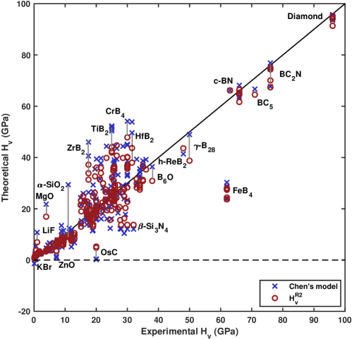
Figure 4: Assessment of the Chen’s model [Eq. (1)] and the model in Eq. (4) for the full dataset including $T^{A}$, $T^{B}$ and $T^{C}$.

To build a more broadly transferable hardness model, we combined all the data in $T^{A}$, $T^{B}$ and $T^{C}$ and randomly divided them into two parts with 90% of the data for the symbolic regression and the remaining data for validating the model. After repeating the regression several times, the optimal regression model in terms of accuracy and simplicity was selected and expressed as

$$H^{\rm R2}_{V}=0.16k^{1/2}G.$$ (4)

Again, the Pugh’s modulus ratio $k=G/B$ is naturally included by the symbolic regression.

Figure 4 assesses the performance of the model in Eq. (4) on the full dataset and compares it to the Chen’s model. The MAEs and RMSEs for each individual dataset are given in Table 2. It is evident that $H^{\rm R2}_{V}$ improves upon the Chen’s model in the predictions for $T^{B}$ and $T^{C}$, while the description for $T^{A}$ is somewhat slightly deteriorated. This is, again, due to the fact that the Chen’s model was fitted using only $T^{A}$. One can also observe that the Chen’s model predictions in fact are very accurate for materials in the superhard regime. However, it severely overestimates the hardness values for materials in the intermediate-hard regime, such as transition-metal borides like ZrB₂, TiB₂, HfB₂ and CrB₄. For those materials with small hardness, the Chen’s model tends to underestimate the experimental values and even incorrectly predicts a negative hardness value for KBr. Overall, the model in Eq. (4) is more accurate, yielding relatively smaller MAE and RMSE for the entire dataset as compared to the Chen’s model. Although the above direct comparison between $H^{\rm R2}_{V}$ and the Chen’s model is not so fair, our study highlights the importance of the training data in obtaining a more accurate and transferable model. Furthermore, one can infer that modeling materials with anisotropic elastic properties is more difficult as compared to the cubic systems with isotropic elastic properties. This results in the dominant errors for all the hardness models (see Table 2). It is somewhat surprising that the simplest Teter’s model Teter (1998) also yields an overall good description of the entire dataset $T^{\rm full}$, though it performs worse for the Chen’s dataset $T^{\rm A}$. This is mostly likely due to the strong correlation between $B$ and $G$, as we will show later.

III.2 Modeling fracture toughness of covalent and ionic crystals

Motivated by the success of symbolic regression in modeling the hardness, we now turn to the modeling of fracture toughness using a similar procedure. We employed the same fracture toughness dataset for covalent and ionic crystals from Niu et al. Niu et al. (2019), and took the shear modulus $G$, bulk modulus $B$ and atomic volume $V_{0}$ as input descriptors. Several fracture toughness models were obtained and they were ranked according to the MAE. The optimal fracture toughness model in the spirit of accuracy and simplicity reads

$$K^{R}_{IC}=3.3k^{1/8}B^{5/4}.$$ (5)

Interestingly, this model only involves $G$ and $B$, whereas the atomic volume $V_{0}$ appearing in Eq. (2) is not present here. This can be understood, because the fracture toughness is mainly connected to the elastic properties, and the atomic volume $V_{0}$ in Eq. (2) was simply used to yield the dimension of fracture toughness.

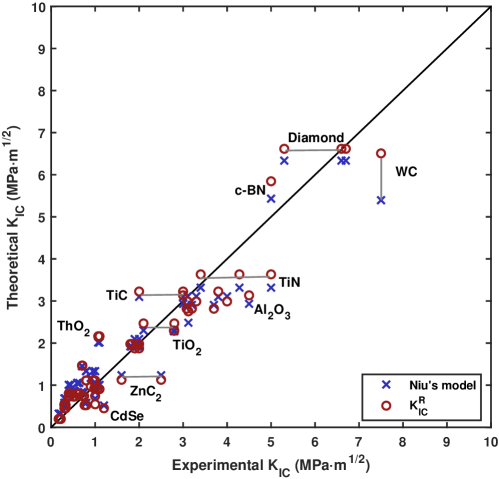
Figure 5: The predicted fracture toughness versus the experimental data using the Niu’s model [Eq. (2)] and the model in Eq. (5). The experimental data are taken from Ref. Niu et al. (2019) and compiled also in Table A4.

Table 3: A summary of MAEs and RMSEs (in MPa$\cdot$m^1/2) of fracture toughness models with respect to the experimental data. In the Oganov’s model Mazhnik and Oganov (2019) $\zeta(\nu)=\frac{1-13.7\nu+48.6\nu^{2}}{1-15.2\nu+70.2\nu^{2}-81.5\nu^{3}}$.

Models	MAE	RMSE
$K^{\rm Niu}_{IC}=V_{0}^{1/6}G(B/G)^{1/2}$ Niu et al. (2019)	0.44	0.60
$K^{\rm Oganov}_{IC}=8840^{-1/2}V_{0}^{1/6}[\zeta(\nu)E]^{3/2}$ Mazhnik and Oganov (2019)	0.35	0.50
$K^{R}_{IC}=3.3k^{1/8}B^{5/4}$ [Eq. (5)]	0.37	0.54

Table A4 of the Appendix collects the experimental fracture toughness data, on which the Niu’s model [Eq. (2)] and the model in Eq. (5) were obtained. The assessment of the two models against the experimental data is shown in Fig. 5. The MAEs and RMSEs of the two models as well as the Oganov’s fracture toughness model Mazhnik and Oganov (2019) are listed in Table 3. It can be seen that all three models reproduce well the experimental data. The model in Eq. (5) is only slightly improved upon the Niu’s model, as manifested by its smaller MAEs and RMSEs (see Table 3). We note that the robustness and transferability of the model needs to be carefully examined due to the limited experimental data. This should hold for the Niu’s model and Oganov’s model as well.

III.3 Predictions of superhard materials with good fracture toughness

Figure 6: (a) Predicted hardness vs. fracture toughness and (b) shear modulus vs. bulk modulus for the 8 062 materials. The dashed line is used to identify the superhard materials (here set to 37 GPa). The color coding in (b) indicates the predicted hardness.

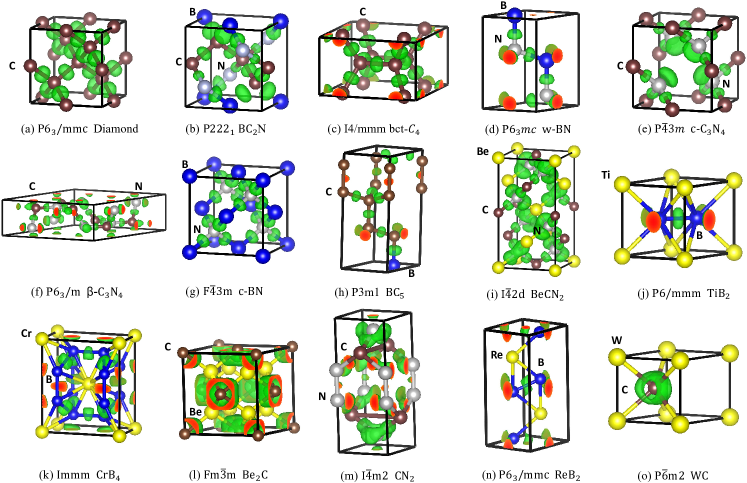
Figure 7: Isosurfaces of electron localization functions with an isovalue of 0.80 for predicted superhard materials. The three-dimensional covalent bonding networks are evident for all materials.

With the accurate and transferable hardness model [Eq. (4)] and fracture toughness model [Eq. (5)] from symbolic regression in hands, we are now in a position to perform high-throughput hardness and fracture toughness predictions. To this aim, we download the shear and bulk moduli of 8 062 materials from the Materials Project website Jain et al. (2013) via Python Materials Genomics (pymatgen) package Ong et al. (2013). The predicted hardness vs. fracture toughness are shown in Fig. 6(a). One can see that in addition to the known superhard materials (e.g., diamond-carbon, metastable bct-C₄ Wei et al. (2010); Xu et al. (2010), BCN₂ Lambrecht and Segall (1992); Hui-Yang et al. (2011), CrB₄ Niu et al. (2012c), etc.) used for training the model, several new potentially superhard materials (marked in blue color) have been predicted. Interestingly, most of them belong to carbon nitrides, carbides, and transition-metal borides. For instance, C₃N₄ He et al. (2006) and Be₂C Kalarasse and Bennecer (2008) have been theoretically predicted to be superhard. The isosurfaces of electron localization functions for these materials are shown in Fig. 7, exhibiting a common feature of three-dimensional covalent bonding networks. Among these superhard materials, many of them exhibit good fracture toughness as well, such as diamond-carbon, bct-C₄, BC₂N, c-C₃N₄, c-BN, and so on. It should be noted that the fracture toughness model [Eq. (5)] only applies to covalent and ionic crystals, and would fail for metals and alloys. However, this is not a big problem here, since we are only interested in the superhard regime where most of materials are covalent and ionic crystals. Finally, it is instructive to plot the predicted hardness as a function of $G$ and $B$. This is done in Fig. 6(b) with the color coding indicating the predicted hardness. One can see that there is a strong correlation between the shear modulus and bulk modulus. This might explain why the simplest Teter’s model Teter (1998) involving only $G$ also works remarkably well (see Table 2).

III.4 Machine learning bulk and shear moduli

As mentioned before, the hardness model [Eq. (4)] and fracture toughness model [Eq. (5)] only require two input quantities, namely, $G$ and $B$. Although they can be routinely calculated from first-principles, the calculations for a large mount of materials still represent a big computational effort. By contrast, machine learning methods run many orders of magnitude faster than DFT calculations, and allow one to efficiently establish the relationship between properties and atomic structure with high precision Xie and Grossman (2017); Avery et al. (2019); Choudhary and DeCost (2021); Das et al. (2022); Mazhnik and Oganov (2020); Chen et al. (2019b).

So far, several machine learning methods have been developed to predict properties of crystalline and molecular materials simply from the structural information. The successful models include, e.g., crystal graph convolutional neural network (CGCNN) Xie and Grossman (2017), atomistic line graph neural network (ALIGNN) Choudhary and DeCost (2021), and crystal explainable property predictor (CrysXPP) Das et al. (2022). From the perspective of building descriptors, CGCNN, and CrysXPP primarily reply on atomic distances, while ALIGNN captures the many-body interactions using GCNN. These methods differ also in input data processing and working paradigm. Specifically, CGCNN generates crystal graphs from crystal materials and builds a graph convolution based supervised model Xie and Grossman (2017). ALIGNN presents a GNN architecture that performs message passing on both the interatomic bond graph and its line graph corresponding to bond angles, leading to improved performance on multiple atomistic prediction tasks Choudhary and DeCost (2021). CrysXPP first learns large amounts of crystal data through an autoencoder (CrysAE), and the learned information is then used to build a property predictor (CrysXPP) Das et al. (2022).

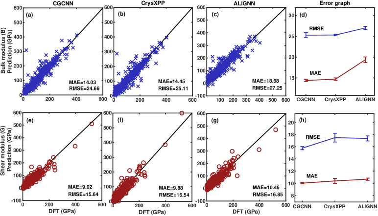
Figure 8: (d)-(h) The validation MAEs and RMSEs for the three considered deep learning models (CGCNN, CrysXPP and ALIGNN) in predicting $B$ and $G$ with respect to the ground truth from DFT calculations. The predicted $B$ ($G$) vs. DFT calculated ones for each model with the lowest errors are shown in (a)-(g).

Here, we employed these three advanced deep learning models to predict $G$ and $B$ of materials and assessed their performance. The $G$ and $B$ data of 8 062 materials were taken from the Materials Project Jain et al. (2013). In order to make a fair assessment on the performance of different models, the same 7 562 structural data were used for training, while the remaining 500 data were used as a test dataset. For the CrysXPP, the structure and energy properties were learned through CrysAE using more than 30 000 data from the Materials Project Jain et al. (2013). Note that the 500 structures in the test dataset were not used in this step. Then, the $G$ and $B$ of 7 562 structures were used to build CrysSPP. For each considered deep learning models, four independent trainings were performed. Figs. 8(d) and (h) display the validation MAEs and RMSEs of the three models in predicting $B$ and $G$, respectively. One can observe that the CGCNN seems to perform best among the three models. The CrysXPP performs almost equally well as the CGCNN, while the ALIGNN is the worst with the largest validation errors for both $B$ and $G$. Moreover, we found that the convergence of ALIGNN is much slower than the other two models, making the CGCNN and CrysXPP stand out for efficient and accurate prediction of shear and bulk moduli.

IV Conclusions

In conclusion, we have built an improved macroscopic hardness model and fracture toughness model by means of an unbiased symbolic regression technique. The obtained models are simple, accurate, and transferable. This is achieved by extending the existing training dataset, incorporating also materials with anisotropic elastic properties, and comparing the widely used semiempirical Chen’s hardness and Niu’s fracture toughness models. Furthermore, we have assessed deep learning models for efficient and accurate prediction of shear and bulk moduli. The developed hardness and fracture toughness predictions models combined with efficient ML-learned bulk and shear moduli allow us to fast screen out potential superhard materials with good fracture toughness through high-throughput calculations.

V Acknowledgments

This work was supported by the National Key R&D Program of China (Grant No. 2021YFB3501503), the National Natural Science Foundation of China (Grant No. 52201030, Grant No. 52188101), the National Science Fund for Distinguished Young Scholars (No. 51725103), and Chinese Academy of Sciences (No. ZDRW-CN-2021-2-5). All calculations were performed on the high performance computational cluster at the Shenyang National University Science and Technology Park.

*

Appendix A Summary of experimental data on hardness and fracture toughness

Table A1: A summary of material name, shear modules ($G$, in GPa), bulk modules ($B$, in GPa), experimental hardness ($H^{\rm exp}_{V}$, in GPa), predicted hardness using the Chen’s model ($H^{\rm Chen}_{V}$, in GPa) and the model in Eq. (4) ($H^{\rm R2}_{V}$, in GPa), and structure type for the dataset $T^{A}$. This is the same dataset as was used in the Chen’s work Chen et al. (2011a), most of which are cubic structures.

	Material	$G$	$B$	$H^{\rm exp}_{V}$	$H^{\rm Chen}_{V}$	$H^{\rm R2}_{V}$	Structure
1	DiamondChen et al. (2011a)	535.5	442.3	96	95.7	94.3	cubic
		548.3	465.5	96	93.9	95.2	cubic
		520.3	431.9	96	94.4	91.4	cubic
		535.0	443.0	96	96.6	94.1	cubic
2	BC2NChen et al. (2011a)	446.0	403.0	76	76.9	75.1	cubic
		445.0	408.0	76	75.4	74.4	cubic
	BC2NJiang et al. (2011)	414.0	400.0	76	67.7	67.4	cubic
		414.0	370.0	76	74.5	70.1	cubic
3	BC5Chen et al. (2011a)	394.0	376.0	71	66.7	64.5	cubic
4	c-BNChen et al. (2011a)	405.4	400.0	66	65.1	65.3	cubic
		403.4	403.7	66	63.8	64.5	cubic
		382.2	375.7	66	63.1	61.7	cubic
		404.4	384.0	66	68.2	66.4	cubic
5	BN Jiang et al. (2011)	409.0	400.0	63	66.2	66.2	cubic
6	$\gamma$-B28Chen et al. (2011a)	236.0	224.0	50	49.0	38.8	cubic
7	B6OChen et al. (2011a)	204.0	228.0	38	36.4	30.9	trigonal
		204.0	228.0	35	36.4	30.9	trigonal
8	$\beta$-SiCChen et al. (2011a)	191.4	224.7	34	32.8	28.3	cubic
		196.6	224.9	34	34.5	29.4	cubic
		190.2	209.2	34	35.5	29.0	cubic
		186.5	220.3	34	32.1	27.5	cubic
9	SiCJiang et al. (2011)	196.0	226.0	26	34.1	29.2	cubic
10	SiO2Chen et al. (2011a)	220.0	305.0	33	29.0	29.9	cubic
	SiO2Mazhnik and Oganov (2019)	233.1	324.1	33	30.0	31.6	cubic
11	ReB2Chen et al. (2011a)	273.0	382.0	30	32.9	36.9	hexagonal
	ReB2Gu et al. (2008),Wang et al. (2018)	304.2	360.0	26.6	43.6	44.7	hexagonal
		283.0	350.0	26.6	39.4	40.7	hexagonal
12	WCChen et al. (2011a)	301.8	438.9	30	33.4	40.0	hexagonal
		282.0	439.0	30	29.3	36.2	hexagonal
13	B4CChen et al. (2011a)	192.0	226.0	30	32.8	28.3	trigonal
	B4CJiang et al. (2011)	171.0	247.0	30	23.3	22.8	trigonal
14	VCChen et al. (2011a)	209.1	305.5	29	26.2	27.7	cubic
15	VC0.88Jiang et al. (2011)	160.0	398.0	29	10.4	16.2	cubic
16	ZrCChen et al. (2011a)	169.7	223.1	25.8	26.3	23.7	cubic
		182.5	228.3	25.8	29.4	26.1	cubic
		185.9	228.0	25.8	30.5	26.9	cubic
		169.6	223.3	25.8	26.2	23.6	cubic
		166.0	223.0	25.8	25.2	22.9	cubic
	ZrCJiang et al. (2011)	160.0	223.3	25.8	23.4	21.7	cubic
17	TiCChen et al. (2011a)	182.2	242.0	24.7	27.1	25.3	cubic
		176.9	250.3	24.7	24.5	23.8	cubic
		198.3	286.0	24.7	25.8	26.4	cubic
		187.8	241.7	24.7	28.8	26.5	cubic
	TiCJiang et al. (2011)	188.0	241.0	28.5	29.0	26.6	cubic
18	TiNChen et al. (2011a)	183.2	282.0	23	22.4	23.6	cubic
		187.2	318.3	23	19.9	23.0	cubic
		205.8	294.6	23	26.7	27.5	cubic
		207.9	326.3	23	23.8	26.6	cubic
	TiNJiang et al. (2011)	160.0	292.0	20	16.3	18.9	cubic
19	RuO2Chen et al. (2011a)	142.2	251.3	20	15.7	17.1	cubic
		173.0	248.0	20	23.7	23.1	cubic
20	AlO2Chen et al. (2011a)	161.0	240.0	20	21.5	21.1	orthorhombic
		160.0	259.0	20	19.2	20.1	orthorhombic
		164.0	254.0	20	20.7	21.1	orthorhombic
		162.0	246.0	20	21.1	21.0	orthorhombic
21	NbCChen et al. (2011a)	171.0	333.0	18	15.6	19.6	cubic
		171.7	340.0	18	15.2	19.5	cubic
	NbCJiang et al. (2011)	150.0	340.0	18.8	11.4	15.9	cubic
22	AlNChen et al. (2011a)	134.7	206.0	18	18.4	17.4	cubic
		130.2	212.1	18	16.5	16.3	cubic
		123.3	207.5	18	15.2	15.2	cubic
		132.0	211.1	18	17.1	16.7	cubic
		128.0	203.0	18	16.9	16.3	cubic
	AlNJiang et al. (2011)	114.8	202.0	18	13.6	13.8	cubic
23	NbNChen et al. (2011a)	155.9	292.0	17	15.4	18.2	cubic
		156.0	315.0	17	13.9	17.6	cubic
	NbNJiang et al. (2011)	165.0	292.0	20	17.3	19.8	cubic
24	HfNChen et al. (2011a)	186.3	315.5	17	20.0	22.9	cubic
		164.8	278.7	17	18.4	20.3	cubic
	HfNJiang et al. (2011)	202.0	306.0	19.5	24.5	26.3	cubic
25	GaNChen et al. (2011a)	105.2	175.9	15.1	13.7	13.0	cubic
		120.0	210.0	15.1	14.1	14.5	cubic
	GaNJiang et al. (2011)	123.7	160.0	20	21.8	17.4	cubic
26	ZrO2Chen et al. (2011a)	88.0	187.0	13	8.4	9.7	cubic
		93.0	187.0	13	9.5	10.5	cubic
	ZrO2Jiang et al. (2011)	80.1	185.0	13	6.8	8.4	cubic
27	SiChen et al. (2011a)	66.6	97.9	12	11.9	8.8	cubic
		64.0	97.9	12	10.9	8.3	cubic
		63.2	90.7	12	11.8	8.4	cubic
		61.7	96.3	12	10.2	7.9	cubic
		61.7	89.0	12	11.5	8.2	cubic
	SiJiang et al. (2011)	68.0	98.0	11.3	12.4	9.1	cubic
28	GaPChen et al. (2011a)	55.7	88.2	9.5	9.3	7.1	cubic
		55.8	88.8	9.5	9.2	7.1	cubic
		56.1	88.6	9.5	9.4	7.1	cubic
		61.9	89.7	9.5	11.5	8.2	cubic
29	AlPChen et al. (2011a)	49.0	86.0	9.4	7.1	5.9	cubic
		51.8	90.0	9.4	7.5	6.3	cubic
		48.8	86.0	9.4	7.0	5.9	cubic
	AlPMazhnik and Oganov (2019)	46.8	81.9	6.5	6.9	5.7	cubic
30	InNChen et al. (2011a)	55.0	123.9	9	5.1	5.9	cubic
		77.0	139.6	9	9.7	9.1	cubic
31	GeChen et al. (2011a)	53.1	72.2	8.8	11.3	7.3	cubic
		43.8	60.3	8.8	9.6	6.0	cubic
	GeJiang et al. (2011)	57.0	71.0	8.8	13.5	8.2	cubic
32	GaAsChen et al. (2011a)	46.5	75.0	7.5	7.8	5.9	cubic
		46.7	75.5	7.5	7.8	5.9	cubic
		46.7	75.4	7.5	7.8	5.9	cubic
33	YO2Chen et al. (2011a)	72.5	166.0	7.5	6.3	7.7	monoclinic
		62.7	146.5	7.5	5.3	6.6	monoclinic
		66.5	149.3	7.5	6.0	7.1	monoclinic
34	InPChen et al. (2011a)	34.3	71.1	5.4	3.7	3.8	cubic
		34.4	72.5	5.4	3.6	3.8	cubic
35	AlAsChen et al. (2011a)	44.8	77.9	5	6.7	5.4	cubic
		44.6	78.3	5	6.5	5.4	cubic
36	GaSbChen et al. (2011a)	34.2	56.3	4.5	5.8	4.3	cubic
		34.1	56.4	4.5	5.8	4.2	cubic
		34.3	56.3	4.5	5.9	4.3	cubic
37	AlSbChen et al. (2011a)	31.5	56.1	4	4.7	3.8	cubic
		31.9	58.2	4	4.5	3.8	cubic
		32.5	59.3	4	4.6	3.8	cubic
		31.9	58.2	4	4.5	3.8	cubic
38	InAsChen et al. (2011a)	29.5	57.9	3.8	3.6	3.4	cubic
		29.5	59.1	3.8	3.4	3.3	cubic
39	InSbChen et al. (2011a)	23.0	46.9	2.2	2.4	2.6	cubic
		22.9	46.5	2.2	2.5	2.6	cubic
		22.9	46.0	2.2	2.5	2.6	cubic
40	ZnSChen et al. (2011a)	32.8	78.4	1.8	2.6	3.4	cubic
		31.5	77.1	1.8	2.3	3.2	cubic
41	ZnSeChen et al. (2011a)	28.8	63.1	1.4	2.7	3.1	cubic
42	ZnSeChen et al. (2011a)	23.4	51.0	1	2.1	2.5	cubic

Table A2: Same as Table LABEL:tab:TA but for the dataset $T^{B}$. This dataset contains additional cubic systems that were not included in the Chen’s work Chen et al. (2011a). The values of shear and bulk moduli with asterisk are taken from the Materials Project Jain et al. (2013).

	Material	$G$	$B$	$H^{\rm exp}_{V}$	$H^{\rm Chen}_{V}$	$H^{\rm R2}_{V}$	Structure
1	$\alpha$-BJiang et al. (2011)	204.5	224.0	35	37.4	31.3	cubic
2	$\gamma-$Si3N4Ying-chun et al. (2012)	249.0*	293.0*	35	38.3	36.7	cubic
		249.0*	293.0*	30	38.7	36.7	cubic
3	BPJiang et al. (2011)	174.0	169.0	33	39.3	28.2	cubic
4	TaCJiang et al. (2011)	190.0	283.3	29	24.0	24.9	cubic
5	ZrB12Wang et al. (2018)	199.0	236.0	27	33.2	29.2	cubic
6	AlB12Jiang et al. (2011)	163.0	139.0	26	44.4	28.2	cubic
7	TaB2Jiang et al. (2011)	228.0	315.0	25.6	29.8	31.0	cubic
	TaB2Jiang et al. (2011)	218.0	360.0	25.6	23.0	27.1	cubic
8	HfCJiang et al. (2011)	180.0	242.7	25.5	26.4	24.8	cubic
	HfCMazhnik and Oganov (2019)	179.2	238.9	19	26.7	24.8	cubic
9	OsCYang and Gao (2010)	72.0	409.0	20	0.2	4.8	cubic
		78.0	438.0	20	0.4	5.3	cubic
10	Si3N4Jiang et al. (2011)	123.0	249.0	19	11.6	13.8	cubic
11	BAsŠimůnek and Vackář (2006)	124.0*	128.0*	19	29.3	19.5	cubic
12	Re2CZhao et al. (2010)	246.3	388.9	17.5	26.4	31.4	cubic
13	MgB2Jiang et al. (2011)	117.5	145.0	17.4	22.4	16.9	cubic
14	VNTian et al. (2012)	165.0*	319.0*	15.2	15.3	19.0	cubic
15	CrNTian et al. (2012)	87.0*	181.0*	11	8.6	9.7	cubic
16	Y2O3Mazhnik and Oganov (2019)	61.1	140.4	6.4	5.4	6.4	cubic
17	MgOTian et al. (2012)	119.0*	151.0*	3.9	21.8	16.9	cubic
18	LiFTian et al. (2012)	51.0*	70.0*	1	10.8	7.0	cubic
19	CdTeMazhnik and Oganov (2019)	14.0	35.0	0.6	0.2	1.4	cubic
		14.0	34.3	0.6	0.3	1.4	cubic
20	NaFTian et al. (2012)	30.0*	48.0*	0.6	5.4	3.8	cubic
21	NaClŠimůnek and Vackář (2006)	14.0*	23.0*	0.3	2.2	1.7	cubic
22	KClŠimůnek and Vackář (2006)	9.0*	16.0*	0.2	0.7	1.1	cubic
	KClTian et al. (2012)	9.0*	16.0*	0.13	0.7	1.1	cubic
23	KBrTian et al. (2012)	7.0*	22.0*	0.1	-1.4	0.6	cubic

Table A3: Same as Table LABEL:tab:TA but for the dataset $T^{C}$. This dataset contains only non-cubic systems. The values of shear and bulk moduli with asterisk are taken from the Materials Project Jain et al. (2013).

	Material	$G$	$B$	$H^{\rm exp}_{V}$	$H^{\rm Chen}_{V}$	$H^{\rm R2}_{V}$	Structure
1	FeB4Gou et al. (2013)	198.0Ma et al. (2019a)	252.0	62	30.3	28.1	orthorhombic
		198.0Ma et al. (2019a)	264.7Ma et al. (2019a)	62	28.4	27.4	orthorhombic
	FeB4Zhang et al. (2017)	177.0	253.0	62	24.2	23.7	orthorhombic
		199.0	263.0	62	28.9	27.7	orthorhombic
		186.0	277.0	62	23.7	24.4	orthorhombic
2	ReB2Jiang et al. (2011)	302.0	371.0	48	41.4	43.6	hexagonal
3	MnB4Zhang et al. (2017)	235.0	266.0	36	39.2	35.3	monoclinic
4	MnB4Ma et al. (2019a)	240.7	274.6	20.1	39.4	36.1	orthorhombic
5	$\beta-$Si3N4Gao et al. (2003)	120.0*	234.0*	32	12.1	13.7	hexagonal
		120.0*	234.0*	30	12.1	13.7	hexagonal
		120.0*	234.0*	28	12.1	13.7	hexagonal
6	HfB2Zhang et al. (2017)	228.0	210.3	31.5	49.7	38.0	hexagonal
	HfB2Gan et al. (2021)	227.0	260.0	21.5	37.8	33.9	hexagonal
		239.0	270.0	21.5	39.7	36.0	hexagonal
7	TiB2Jiang et al. (2011)	263.0	244.0	31.5	53.9	43.7	hexagonal
	TiB2Gan et al. (2021)	258.0	250.0	25	50.4	41.9	hexagonal
		270.0	260.0	25	52.3	44.0	hexagonal
	TiB2Wang et al. (2018)	255.0	240.0	25	51.9	42.1	hexagonal
		260.0	250.0	25	51.2	42.4	hexagonal
8	CrB4Zhang et al. (2017)	296.0	290.0	30	54.2	47.8	orthorhombic
		259.0	275.0	30	45.1	40.2	orthorhombic
	CrB4Šimunek and Dušek (2017)	258.0*	277.0*	28.6	44.4	39.8	orthorhombic
		258.0*	277.0*	23.3	44.4	39.8	orthorhombic
9	ZrB2Jiang et al. (2011)	221.0	218.0	30	44.8	35.6	hexagonal
	ZrB2Gan et al. (2021)	218.0	231.0	17.5	40.6	33.9	hexagonal
		231.0	228.0	17.5	46.0	37.2	hexagonal
10	OsB2Mazhnik and Oganov (2019)	167.9	293.8	29.4	17.8	20.3	orthorhombic
	OsB2Jiang et al. (2011)	161.0	297.0	21.6	16.1	19.0	orthorhombic
	OsB2Šimunek and Dušek (2017)	166.0*	311.0*	24.9	16.1	19.4	orthorhombic
		166.0*	311.0*	16.8	16.1	19.4	orthorhombic
	OsB2Gu et al. (2008)	166.0*	311.0*	23.5	16.1	19.4	orthorhombic
11	ZrNJiang et al. (2011)	160.0	267.0	27	18.4	19.8	hexagonal
	ZrNMazhnik and Oganov (2019)	75.2	196.1	12	5.2	7.4	hexagonal
12	WB2(hP6)Šimunek and Dušek (2017)	141.0	295.0	27.7	12.2	15.6	hexagonal
	WB2Wang et al. (2018)	200.0	349.0	26.5	20.1	24.2	hexagonal
		207.0	318.0	26.5	24.4	26.7	hexagonal
	WB2(hP12)Šimunek and Dušek (2017)	224.0*	321.0*	22.2	28.1	29.9	hexagonal
13	C40-NbSi2Pu and Pan (2021)	143.0	175.0	27.5	25.8	20.7	hexagonal
14	VB2Wang et al. (2018)	245.0	284.0	25.8	39.0	36.4	hexagonal
		241.0	282.0	25.8	38.2	35.6	hexagonal
15	WB3Wang et al. (2018)	249.0	326.0	25.5	33.8	34.8	hexagonal
		245.0	293.0	25.5	37.5	35.8	hexagonal
16	MoB2Wang et al. (2018)	186.0	296.0	25.1	21.7	23.6	orthorhombic
		231.0	303.0	25.1	32.1	32.3	orthorhombic
17	MoB2Šimunek and Dušek (2017)	225.0*	295.0*	21.2	31.6	31.4	trigonal
18	Mo2BŠimunek and Dušek (2017)	141.0*	293.0*	24.5	12.4	15.7	tetragonal
19	RuB2Kanoun et al. (2010)	179.2	289.1	24.2	20.8	22.6	orthorhombic
	RuB2Jiang et al. (2011)	144.0	265.0	19.2	14.9	17.0	orthorhombic
	RuB2Mazhnik and Oganov (2019)	183.5	291.7	15.1	21.5	23.3	orthorhombic
20	CrB2Wang et al. (2018)	170.0	295.0	22.1	18.2	20.6	tetragonal
21	CrB2Šimunek and Dušek (2017)	183.0*	252.0*	15.8	26.0	25.0	hexagonal
22	TaNTian et al. (2012)	182.0*	307.0*	22	19.8	22.4	hexagonal
23	Al2O3Jiang et al. (2011)	162.0	246.0	21.5	21.1	21.0	trigonal
		165.0	250.6	17.8	21.3	21.4	trigonal
24	CrBŠimunek and Dušek (2017)	223.0*	266.0*	19.6	35.5	32.7	orthorhombic
25	Si2N2OYing-chun et al. (2012)	93.1	119.2	19	18.3	13.2	orthorhombic
26	Mn3B4Ma et al. (2019b)	173.3	254.0	16.3	23.1	22.9	orthorhombic
27	BeOMazhnik and Oganov (2019)	155.0	206.7	15	24.3	21.5	hexagonal
	BeOMazhnik and Oganov (2019)	155.0	206.7	13Gao et al. (2003)	24.3	21.5	hexagonal
28	$\alpha-$SiO2Gao et al. (2003)	44.0	27.0	11	29.4	9.0	trigonal
29	ZnOJiang et al. (2011)	41.0	148.0	7.2	0.9	3.5	hexagonal
	ZnOMazhnik and Oganov (2019)	40.8	132.1	7.2	1.4	3.6	hexagonal

Table A4: The predicted fracture toughness (in MPa$\cdot$m^1/2) of covalent and ionic crystals using the Niu’s model [Eq. (2)] and the model in Eq. (5) as compared to the experimental data. The data of elastic moduli ($G$ and $B$) and atomic volume ($V_{0}$) are taken from Ref. Niu et al. (2019).

	Material	G (GPa)	B (GPa)	$V_{0}$ ($\AA^{3}/{\rm atom}$)	$K_{IC}^{\rm exp}$	$K_{IC}^{\rm Niu}$	$K_{IC}^{\rm R}$
1	Diamond	520.3	431.9	5.70	5.3, 6.6, 6.7Niu et al. (2019)	6.34	6.62
2	WC	301.8	438.9	10.61	7.5Niu et al. (2019)	5.40	6.51
3	c-BN	403.4	403.7	5.95	5Niu et al. (2019)	5.43	5.85
4	TiN	183.2	282	9.66	3.4, 4.28, 5.0Niu et al. (2019)	3.32	3.63
5	TiC	176.9	250.3	10.19	2-3, 3.8Niu et al. (2019)	3.10	3.23
6	$\beta-$SiC	196.6	224.9	10.49	3.1, 3.3, 4.0Niu et al. (2019)	3.11	2.99
7	Al2O3	164.3	254.3	8.75	3-4.5Mazhnik and Oganov (2019)	2.93	3.13
8	B4C	191.9	225.8	7.42	3.08, 3.2, 3.7Niu et al. (2019)	2.90	2.82
9	AlN	122.1	194.1	10.63	2.79Niu et al. (2019)	2.28	2.30
10	TiO2	110.1	209.2	12.22	2.1, 2.8Niu et al. (2019)	2.30	2.47
11	$\alpha$-Si3N4	120.1	223.8	10.62	3.12Niu et al. (2019)	2.48	2.75
12	MgO	130.3	158.3	9.67	1.9, 2.0Niu et al. (2019)	2.09	1.87
13	ThO2	88.1	187.7	14.79	1.07Niu et al. (2019), 1.1Mazhnik and Oganov (2019)	2.01	2.16
14	MgAl2O4	96.1	180.2	9.73	1.83, 1.94, 1.97Niu et al. (2019)	1.92	1.98
15	Y2O3	61.3	138.5	15.33	0.71Niu et al. (2019)	1.45	1.46
16	ZnO2	62.1	113.8	10.15	1.6, 2.5Niu et al. (2019)	1.23	1.13
17	Si	66.3	162	20.41	0.79, 0.95Niu et al. (2019)	1.33	1.11
18	GaP	55.8	88.8	21.18	0.9Niu et al. (2019)	1.17	0.97
19	Ge	53.1	72.2	24.17	0.59-0.64Niu et al. (2019), 0.6Mazhnik and Oganov (2019)	1.05	0.80
20	MgF2	52.2	95.3	11.36	0.98Niu et al. (2019)	1.06	0.92
21	GaAs	46.7	75.5	23.92	0.44Niu et al. (2019)	1.01	0.80
22	BaTiO3	45.1	94.9	13.15	1.05Niu et al. (2019)	1.01	0.91
23	InP	34.3	72.5	26.99	0.42-0.53Niu et al. (2019)	0.86	0.73
24	ZnS	32.8	78.4	20.21	0.75, 1Niu et al. (2019), 0.7-1Mazhnik and Oganov (2019)	0.84	0.74
25	ZnSe	28.1	58.4	23.60	0.32, 1Niu et al. (2019)	0.69	0.55
26	CdS	18.6	61.1	26.07	0.33, 0.76Niu et al. (2019)	0.58	0.52
27	CdSe	16.3	53.1	29.79	0.33-1.2Niu et al. (2019)	0.52	0.45
28	NaCl	14.8	24.9	22.61	0.17-0.22Niu et al. (2019), 0.2Mazhnik and Oganov (2019)	0.32	0.20

References

- Haines et al. (2001) J. Haines, J.-M. Leger, and G. Bocquillon, Annual Review of Materials Research 31, 1 (2001).
- Xu and Tian (2015) B. Xu and Y. Tian, Science China Materials 58, 132 (2015).
- Gilman et al. (2006) J. J. Gilman, R. W. Cumberland, and R. B. Kaner, International Journal of Refractory Metals & Hard Materials 24, 1 (2006).
- Ivanovskii (2011) A. L. Ivanovskii, Journal of Superhard Materials 33, 73 (2011).
- Riedel (1994) R. Riedel, Advanced Materials 6, 549 (1994).
- Mao et al. (2003) W. L. Mao, H. kwang Mao, P. J. Eng, T. P. Trainor, M. Newville, C. chang Kao, D. L. Heinz, J. Shu, Y. Meng, and R. J. Hemley, Science 302, 425 (2003).
- Li et al. (2009) Q. Li, Y. Ma, A. R. Oganov, H. Wang, H. Wang, Y. Xu, T. Cui, H. kwang Mao, and G. Zou, Physical review letters 102 17, 175506 (2009).
- Niu et al. (2012a) H. Niu, X.-Q. Chen, S. Wang, D. Li, W. L. Mao, and Y. Li, Phys. Rev. Lett. 108, 135501 (2012a).
- Avery et al. (2019) P. Avery, X. Wang, C. Oses, E. Gossett, D. M. Proserpio, C. Toher, S. Curtarolo, and E. Zurek, npj Computational Materials 5, 1 (2019).
- Cheng et al. (2013) X. Cheng, W. Zhang, X.-Q. Chen, H. Niu, P. Liu, K. Du, G. Liu, D. Li, H.-M. Cheng, H. Ye, and Y. Li, Applied Physics Letters 103, 171903 (2013).
- Dong et al. (2018) H. Dong, A. Oganov, V. Brazhkin, Q. Wang, J. Zhang, M. Davari, X.-F. Zhou, F. Wu, and Q. Zhu, Physical Review B 98, 1 (2018).
- Zhao et al. (2018) C. Zhao, Y. Duan, J. Gao, W. Liu, H. Dong, H. Dong, D. Zhang, and A. R. Oganov, Phys. Chem. Chem. Phys. 20, 24665 (2018).
- Bykova et al. (2022) E. Bykova, S. V. Ovsyannikov, M. Bykov, Y. Yin, T. Fedotenko, H. Holz, S. Gabel, B. Merle, S. Chariton, V. B. Prakapenka, N. Dubrovinskaia, A. F. Goncharov, and L. Dubrovinsky, J. Mater. Chem. A 10, 20111 (2022).
- Chuvil’deev et al. (2015) V. N. Chuvil’deev, Y. V. Blagoveshchenskii, M. S. Boldin, N. Sakharov, A. V. Nokhrin, N. V. Isaeva, S. V. Shotin, Y. G. Lopatin, O. A. Belkin, and E. S. Smirnova, Technical Physics Letters 41, 397 (2015).
- Sung and Tai (1997) C. M. Sung and M. F. Tai, International Journal of Refractory Metals & Hard Materials 15, 237 (1997).
- Gao et al. (2020) C. L. Gao, W. Wu, J. D. Shi, Z. Y. Xiao, and A. Akbarzadeh, Additive manufacturing 34, 101378 (2020).
- Ivashchenko et al. (2015) V. Ivashchenko, S. Vepřek, A. S. Argon, P. E. A. Turchi, L. Gorb, F. Hill, and J. Leszczynski, Thin Solid Films 578, 83 (2015).
- Tian et al. (2013) Y. Tian, B. Xu, D. Yu, Y. Ma, Y. Wang, Y. B. Jiang, W. Hu, C. Tang, Y. Gao, K. Luo, Z. Zhao, L.-M. Wang, B. Wen, J. He, and Z. Liu, Nature 493, 385 (2013).
- Li et al. (2015) Y. Li, J. Hao, H. Liu, S. Lu, and J. S. Tse, Physical review letters 115 10, 105502 (2015).
- Zhao et al. (2016) Z. Zhao, B. Xu, and Y. Tian, Annual Review of Materials Research 46, 383 (2016).
- Hovsepian (2006) W. D. Hovsepian, P. Eh.and Münz, “Synthesis, structure, and applications of nanoscale multilayer/superlattice structured pvd coatings,” in Nanostructured Coatings, edited by A. Cavaleiro and J. T. M. De Hosson (Springer New York, New York, NY, 2006) pp. 555–644.
- Choudhary et al. (2018) K. Choudhary, G. Cheon, E. Reed, and F. Tavazza, Phys. Rev. B 98, 014107 (2018).
- Kvashnin et al. (2019) A. G. Kvashnin, Z. Allahyari, and A. R. Oganov, Journal of Applied Physics 126, 040901 (2019).
- Mazhnik and Oganov (2020) E. Mazhnik and A. R. Oganov, Journal of Applied Physics 128, 075102 (2020).
- Cole (1957) A. H. Cole, The Journal of Economic History 17, 476–477 (1957).
- Nix and Gao (1998) W. D. Nix and H. Gao, Journal of the Mechanics and Physics of Solids 46, 411 (1998).
- Sun et al. (2022) G. Sun, X. Feng, X. Wu, S. Zhang, and B. Wen, Journal of Materials Science & Technology 114, 215 (2022).
- Li et al. (2010) Q. Li, H. Wang, and Y. Ma, Journal of Superhard Materials 32, 192 (2010).
- Tian et al. (2012) Y. Tian, B. Xu, and Z. Zhao, International Journal of Refractory Metals and Hard Materials 33, 93 (2012).
- Gilman (1973) J. J. Gilman, Journal of Applied Physics 44, 982 (1973).
- Teter (1998) D. M. Teter, MRS Bulletin 23, 22–27 (1998).
- Chen et al. (2011a) X.-Q. Chen, H. Niu, D. Li, and Y. Li, Intermetallics 19, 1275 (2011a).
- Pugh (1954) S. F. Pugh, The London, Edinburgh, and Dublin Philosophical Magazine and Journal of Science 45, 823 (1954).
- Niu et al. (2012b) H. Niu, X.-Q. Chen, P. Liu, W. Xing, X. Cheng, D. Li, and Y. Li, Scientific reports 2, 718 (2012b).
- Senkov and Miracle (2021) O. N. Senkov and D. B. Miracle, Scientific Reports , 1 (2021).
- Chen et al. (2011b) X.-Q. Chen, H. Niu, C. Franchini, D. Li, and Y. Li, Physical Review B 84, 121405 (2011b).
- Zhang et al. (2014) M. Zhang, M. Lu, Y. Du, L. Gao, C. Lu, and H. Liu, The Journal of chemical physics 140, 174505 (2014).
- Zhang et al. (2017) G. Zhang, R. Gao, Y. Zhao, T. Bai, and Y. Hu, Journal of Alloys and Compounds 723, 802 (2017).
- Zhang et al. (2022) J. Zhang, Y. Jin, C. Zhang, Y. Wang, L. Tang, S. Li, M. Ju, J. Wang, W. Sun, and X. Dou, RSC Advances 12, 11722 (2022).