InGram: Inductive Knowledge Graph Embedding via Relation Graphs

Abstract

Inductive knowledge graph completion has been considered as the task of predicting missing triplets between new entities that are not observed during training. While most inductive knowledge graph completion methods assume that all entities can be new, they do not allow new relations to appear at inference time. This restriction prohibits the existing methods from appropriately handling real-world knowledge graphs where new entities accompany new relations. In this paper, we propose an Inductive knowledge Graph embedding method, InGram, that can generate embeddings of new relations as well as new entities at inference time. Given a knowledge graph, we define a relation graph as a weighted graph consisting of relations and the affinity weights between them. Based on the relation graph and the original knowledge graph, InGram learns how to aggregate neighboring embeddings to generate relation and entity embeddings using an attention mechanism. Experimental results show that InGram outperforms 14 different state-of-the-art methods on varied inductive learning scenarios.

1 Introduction

Knowledge graphs represent known facts as a set of triplets, each of which is composed of a head entity, a relation, and a tail entity (Ji et al., 2022). Among various approaches to predicting missing triplets in knowledge graphs, embedding-based methods are known to be effective, where entities and relations are converted into low-dimensional embedding vectors (Nathani et al., 2019). Classical knowledge graph embedding models (Liu et al., 2017; Sun et al., 2019) assume a transductive learning. That is, it is assumed that all entities and relations are observed during training. Transductive knowledge graph embedding methods predict a missing triplet by identifying a plausible combination of the observed entities and relations (Wang et al., 2017).

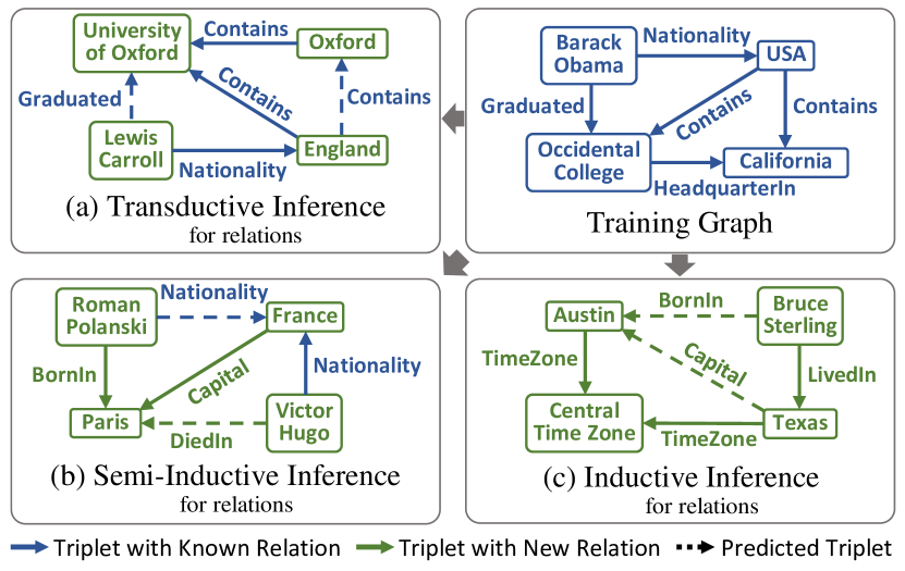
Figure 1: For relations, (a) is a transductive inference, (b) is a semi-inductive inference, and (c) is an inductive inference.

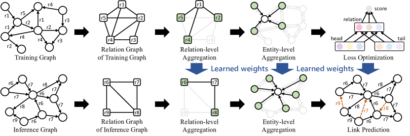
Figure 2: Overview of InGram. Given a knowledge graph, a relation graph is created to define the neighboring relations of each relation. Based on the relation graph and the original knowledge graph, relation and entity embedding vectors are computed by aggregating their neighbors’ embeddings. During training, InGram learns how to aggregate the neighbors’ embeddings by maximizing the scores of training triplets. At inference time, InGram creates embeddings of new relations and entities by aggregating their neighbors’ embeddings and conducts link prediction in the way it learned during training.

In recent years, inductive knowledge graph completion has been studied to predict missing triplets between new entities that are not observed at training time (Teru et al., 2020). If an entity or a relation is observed during training, we call them known and new otherwise; they are sometimes referred to as seen and unseen (Xu et al., 2022). To handle new entities, some methods focus on learning entity-independent relational patterns by logical rule mining (Sadeghian et al., 2019), while others exploit Graph Neural Networks (GNNs) (Yan et al., 2022). However, most existing methods assume that only entities can be new, and all relations should be observed during training. Thus, they perform inductive inference for entities but transductive inference for relations as shown in Figure 1(a).

In this paper, we consider more realistic inductive learning scenarios: (i) the relations at inference time consist of a mixture of known and new relations (semi-inductive inference for relations), or (ii) the relations are all new due to an entirely new set of entities (inductive inference for relations). Figure 1(b) and Figure 1(c) show these scenarios. We propose InGram, an Inductive knowledge Graph embedding method that can generate embedding vectors for new relations and entities only appearing at inference time. Figure 2 shows an overview of InGram when all relations and entities are new. A key idea is to define a relation graph where a node corresponds to a relation, and an edge weight indicates the affinity between relations. Once the relation graph is defined, we can designate neighboring relations for each relation. Given the relation graph and the original knowledge graph, the relation and entity embedding vectors are computed by attention-based aggregations of their neighbors’ embeddings. The aggregation process is optimized to maximize the plausibility scores of triplets in a training knowledge graph. What InGram learns during training is how to aggregate neighboring embeddings to generate the relation and entity embeddings. At inference time, InGram generates embeddings of new relations and entities by aggregating neighbors’ embeddings based on the new relation graph computed from a given inference knowledge graph and the attention weights learned during training.

To the best of our knowledge, InGram is the first method that introduces the relation-level aggregation that allows the model to be generalizable to new relations. Due to the fully inductive capability of InGram, we can generate embeddings by training InGram on a tractable, partially observed set and simply applying it to an entirely new set without retraining. Different from some inductive methods that rely on large language models (Zha et al., 2022), InGram makes inferences solely based on the structure of a given knowledge graph. Experimental results show that InGram significantly outperforms 14 different knowledge graph completion methods in inductive link prediction on 12 datasets with varied ratios of new relations. The performance gap between InGram and the best baseline method is substantial, especially when the ratio of new relations is high, which is a more challenging scenario.

(a) Knowledge Graph

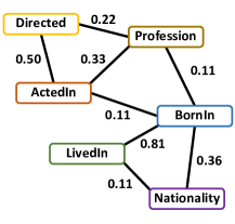
(b) Relation Graph

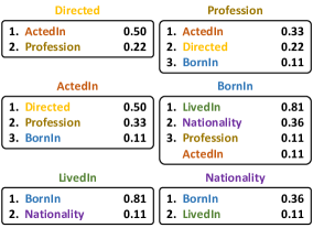
(c) Affinity scores of the relations

Figure 3: Given a knowledge graph, we define a relation graph as a weighted graph where each node indicates a relation, and each edge weight indicates the affinity between two relations. Self-loops in the relation graph are omitted for brevity.

2 Related Work

Rule Mining and Subgraph Reasoning.

For inductive knowledge graph completion, (Yang et al., 2017) and (Sadeghian et al., 2019) have proposed learning first-order logical rules, while (Wang et al., 2021), (Zhu et al., 2021) and (Zhang & Yao, 2022) have considered relational context or paths. GraIL (Teru et al., 2020) has proposed a subgraph-based reasoning framework that extracts subgraphs and scores them using a GNN. Some follow-up works of GraIL include (Mai et al., 2021), (Xu et al., 2022), and (Lin et al., 2022). (Yan et al., 2022) has focused on cycle-based rule learning while (Liu et al., 2021) has proposed GNN-based encoding capturing logical rules. Different from our method, all these methods assume only entities can be new, and relations should be known in advance. (Jin et al., 2022) has recently proposed GraphANGEL handling new relations, but it assumes all entities are known.

Differences between RMPI and InGram.

RMPI (Geng et al., 2023) has concurrently studied the problem of handling new relations, although how RMPI and InGram solve the problem is quite different. While RMPI extracts a local subgraph for every candidate entity to score the corresponding triplet, InGram directly utilizes the whole structure of a given knowledge graph. Also, RMPI uses an unweighted relation view per every individual triplet, whereas InGram defines one global relation graph where weights are important. Due to these fundamental differences, InGram is much more scalable and effective than RMPI. For example, InGram took 15 minutes and RMPI took 52 hours to process NL-100 dataset while InGram achieves much better link prediction performance than RMPI. Details will be discussed in Section 6. Furthermore, RMPI is designed only for knowledge graph completion and does not compute embedding vectors, while InGram returns a set of embedding vectors for entities and relations that can be also utilized in many other downstream tasks.

Reasoning on Evolving Graphs.

Some methods have focused on modeling emerging entities (Hamaguchi et al., 2017; Wang et al., 2022). For example, (Wang et al., 2019) has considered rule and network-based attention weights, and (Dai et al., 2021) has extended RotatE (Sun et al., 2019). All these methods assume that a triplet should be composed of one known entity and one new entity. (Cui et al., 2022) has proposed a GCN-based (Kipf & Welling, 2017) method to more flexibly handle emerging entities. Compared to these methods, we tackle a more challenging problem where all entities are new instead of only some portions being new.

Textual Descriptions and Language Models.

(Daza et al., 2021), (Ali et al., 2021) and (Gesese et al., 2022) have used pre-trained vectors by BERT (Devlin et al., 2019) using textual descriptions. Some methods have utilized language models to handle new entities (Markowitz et al., 2022). For example, (Zha et al., 2022) has leveraged a pre-trained language model and fine-tuned it. All these methods employ a rich language model or require text descriptions that might not always be available. On the other hand, InGram only utilizes the structure of a given knowledge graph.

3 Problem Definition and Setting

In inductive knowledge graph embedding, we are given two graphs: a training graph $\widetilde{G_{\text{tr}}}$ and an inference graph $\widetilde{G_{\text{inf}}}$. A training graph is defined by $\widetilde{G_{\text{tr}}}=(\mathcal{V}_{\text{tr}},\mathcal{R}_{\text{tr}},\mathcal{E}_{\text{tr}})$ where $\mathcal{V}_{\text{tr}}$ is a set of entities, $\mathcal{R}_{\text{tr}}$ is a set of relations, and $\mathcal{E}_{\text{tr}}$ is a set of triplets in $\widetilde{G_{\text{tr}}}$. We divide $\mathcal{E}_{\text{tr}}$ into two disjoint sets such as $\mathcal{E}_{\text{tr}}\coloneqq\mathcal{F}_{\text{tr}}\cup\mathcal{T}_{\text{tr}}$ where $\mathcal{F}_{\text{tr}}$ is a set of known facts and $\mathcal{T}_{\text{tr}}$ is a set of triplets a model is optimized to predict. An inference graph is defined by $\widetilde{G_{\text{inf}}}=(\mathcal{V}_{\text{inf}},\mathcal{R}_{\text{inf}},\mathcal{E}_{\text{inf}})$ where $\mathcal{V}_{\text{inf}}$ is a set of entities, $\mathcal{R}_{\text{inf}}$ is a set of relations, and $\mathcal{E}_{\text{inf}}$ is a set of triplets in $\widetilde{G_{\text{inf}}}$. We partition $\mathcal{E}_{\text{inf}}$ into three pairwise disjoint sets, such that $\mathcal{E}_{\text{inf}}\coloneqq\mathcal{F}_{\text{inf}}\cup\mathcal{T}_{\text{val}}\cup\mathcal{T}_{\text{test}}$ with a ratio of 3:1:1. $\mathcal{F}_{\text{inf}}$ is a set of observed facts where it contains all entities and relations included in $\widetilde{G_{\text{inf}}}$, $\mathcal{T}_{\text{val}}$ is a set of triplets for validation, and $\mathcal{T}_{\text{test}}$ is a set of test triplets. The fact sets $\mathcal{F}_{\text{tr}}$ and $\mathcal{F}_{\text{inf}}$ are also defined in (Zhang & Yao, 2022; Ali et al., 2021). Note that $\mathcal{V}_{\text{tr}}\cap\mathcal{V}_{\text{inf}}=\emptyset$ by following a conventional inductive learning setting (Teru et al., 2020). Most existing methods assume $\mathcal{R}_{\text{inf}}\subseteq\mathcal{R}_{\text{tr}}$ due to the constraint that relations cannot be new at inference time (Zhang & Yao, 2022). On the other hand, in our problem setting, $\mathcal{R}_{\text{inf}}$ is not necessarily a subset of $\mathcal{R}_{\text{tr}}$ since new relations are allowed to appear.

At training time, we use $G_{\text{tr}}\coloneqq(\mathcal{V}_{\text{tr}},\mathcal{R}_{\text{tr}},\mathcal{F}_{\text{tr}})$ and a model is trained to predict $\mathcal{T}_{\text{tr}}$. When tuning the hyperparameters of a model, we use $G_{\text{inf}}\coloneqq(\mathcal{V}_{\text{inf}},\mathcal{R}_{\text{inf}},\mathcal{F}_{\text{inf}})$ to compute the embeddings; we check the model’s performance on $\mathcal{T}_{\text{val}}$. At inference time, we evaluate the model’s performance using $\mathcal{T}_{\text{test}}$. The way we use $\mathcal{F}_{\text{inf}}$, $\mathcal{T}_{\text{val}}$ and $\mathcal{T}_{\text{test}}$ is identical to (Ali et al., 2021; Galkin et al., 2022). For brevity, we do not explicitly mention $G_{\text{tr}}$ or $G_{\text{inf}}$ in the following sections; those should be distinguished in context.

4 Defining Relation Graphs

Let us represent a knowledge graph as $G=(\mathcal{V},\mathcal{R},\mathcal{F})$ where $\mathcal{V}$ is a set of entities, $\mathcal{R}$ is a set of relations, and $\mathcal{F}$ is a set of triplets, i.e., $\mathcal{F}=\{(v_{i},r_{k},v_{j})|v_{i}\in\mathcal{V},r_{k}\in\mathcal{R},v_{j}\in\mathcal{V}\}$. For every $(v_{i},r_{k},v_{j})\in\mathcal{F}$, we add a reverse relation $r_{k}^{-1}$ to $\mathcal{R}$ and add a reverse triplet $(v_{j},r_{k}^{-1},v_{i})$ to $\mathcal{F}$ (Schlichtkrull et al., 2018). Assume that $|\mathcal{V}|=n$ and $|\mathcal{R}|=m$.

Given a knowledge graph, we define a relation graph as a weighted graph where each node corresponds to a relation, and each edge weight indicates the affinity between two relations. Figure 3 shows an example where we omit the reverse relations and self-loops in the relation graph for simplicity. Briefly speaking, we measure the affinity between two relations by considering how many entities are shared between them and how frequently they share the same entity.

To represent which relations are associated with which entities, we create two matrices $\boldsymbol{E}_{\mathrm{h}}\in\mathbb{R}^{n\times m}$ and $\boldsymbol{E}_{\mathrm{t}}\in\mathbb{R}^{n\times m}$ where the subscripts $\mathrm{h}$ and $\mathrm{t}$ indicate head and tail, respectively. Let $\boldsymbol{E}_{\mathrm{h}}[i,j]$ denote the $i$-th row and the $j$-th column element of $\boldsymbol{E}_{\mathrm{h}}$, where $\boldsymbol{E}_{\mathrm{h}}[i,j]$ is the frequency of $v_{i}$ appearing as a head entity of relation $r_{j}$. Similarly, $\boldsymbol{E}_{\mathrm{t}}[i,j]$ is the frequency of $v_{i}$ appearing as a tail entity of relation $r_{j}$. While some entities are frequently involved in relations, some entities are rarely involved in relations. To take this into account, we define the degree of an entity to be the sum of its frequencies. Formally, we define $\boldsymbol{A}_{\mathrm{h}}\coloneqq{\boldsymbol{E}_{\mathrm{h}}}^{T}{\boldsymbol{D}_{\mathrm{h}}}^{-2}\boldsymbol{E}_{\mathrm{h}}$ where ${\boldsymbol{D}_{\mathrm{h}}}\in\mathbb{R}^{n\times n}$ is the degree diagonal matrix of entities for head, i.e., $\boldsymbol{D}_{\mathrm{h}}[i,i]\coloneqq\sum_{j}\boldsymbol{E}_{\mathrm{h}}[i,j]$. Similarly, we define $\boldsymbol{A}_{\mathrm{t}}\coloneqq{\boldsymbol{E}_{\mathrm{t}}}^{T}{\boldsymbol{D}_{\mathrm{t}}}^{-2}\boldsymbol{E}_{\mathrm{t}}$ where ${\boldsymbol{D}_{\mathrm{t}}}\in\mathbb{R}^{n\times n}$ is the degree diagonal matrix of entities for tail. The degree normalization terms allow the sum of the affinity weights introduced by each entity in $\boldsymbol{A}_{\mathrm{h}}$ and $\boldsymbol{A}_{\mathrm{t}}$ to be normalized to one.

Finally, we define the adjacency matrix of the relation graph to be $\boldsymbol{A}\coloneqq\boldsymbol{A}_{\mathrm{h}}+\boldsymbol{A}_{\mathrm{t}}$ where $\boldsymbol{A}\in\mathbb{R}^{m\times m}$ and each element $a_{ij}\in\boldsymbol{A}$ indicates the affinity between the relations $r_{i}$ and $r_{j}$. In Figure 3, we see that the relation graph identifies semantically close relations even though we use only the structure of a knowledge graph. However, there is a chance that we miss some semantically similar relation pairs in the relation graph if they do not share an entity in the knowledge graph. Note that the goal of the relation graph is not to identify the perfect set of similar relations but to define a relation’s reasonable neighborhood whose representation vectors can be used to create the embedding of the target relation, which will be discussed in Section 5.1.

5 InGram: Inductive Knowledge Graph Embedding Model

We present InGram that consists of relation-level aggregation, entity-level aggregation, and modeling of relation-entity interactions.

5.1 Updating Relation Representation Vectors via Relation-Graph-Based Aggregation

Suppose we have an initial feature vector for a relation $r_{i}$, denoted by ${\bf{x}}_{i}\in\mathbb{R}^{d}$ ($i=1,{\cdots},m$), where $d$ is the dimension of a relation vector. We initialize ${\bf{x}}_{i}$ using Glorot initialization (Glorot & Bengio, 2010). Let ${\bf{z}}_{i}^{(l)}\in\mathbb{R}^{d^{\prime}}$ denote a hidden representation of $r_{i}$ where $d^{\prime}$ is the hidden dimension, the superscript $(l)$ indicates the $l$-th layer with $l=0,{\cdots},L-1$, and $L$ is the number of layers for relations. We compute ${\bf{z}}_{i}^{(0)}=\boldsymbol{H}{\bf{x}}_{i}$ where $\boldsymbol{H}\in\mathbb{R}^{d^{\prime}\times d}$ is a trainable matrix that projects the initial feature vector to a hidden representation vector. All vectors are assumed to be column vectors unless specified.

Since we define the relation graph $\boldsymbol{A}$ in Section 4, we can designate the neighboring relations of each relation using $\boldsymbol{A}$. We update each relation’s representation by aggregating its own and neighbors’ representation vectors. Specifically, we define the forward propagation as follows:

$${\bf{z}}_{i}^{(l+1)}=\sigma\left(\sum_{r_{j}\in\mathcal{N}_{i}}\alpha_{ij}^{(l)}\boldsymbol{W}^{(l)}{\bf{z}}_{j}^{(l)}\right)$$ (1)

where $\sigma(\cdot)$ is an element-wise activation function such as LeakyReLU (Maas et al., 2013), ${\bf{z}}_{j}^{(l)}$ is a relation representation vector of $r_{j}$, $\boldsymbol{W}^{(l)}\in\mathbb{R}^{{d^{\prime}}\times{d^{\prime}}}$ is a weight matrix, $\mathcal{N}_{i}$ is the set of neighbors of $r_{i}$ on the relation graph $\boldsymbol{A}$, and the attention value $\alpha_{ij}^{(l)}$ is defined by

$$\alpha_{ij}^{(l)}=\dfrac{\textup{exp}\left({{\bf{y}}}^{(l)}\sigma\left(\boldsymbol{P}^{(l)}[{\bf{z}}_{i}^{(l)}\|{\bf{z}}_{j}^{(l)}]\right)+c_{s(i,j)}^{(l)}\right)}{\sum_{r_{j^{\prime}}\in\mathcal{N}_{i}}\textup{exp}\left({{\bf{y}}}^{(l)}\sigma\left(\boldsymbol{P}^{(l)}[{\bf{z}}_{i}^{(l)}\|{\bf{z}}_{j^{\prime}}^{(l)}]\right)+c_{s(i,j^{\prime})}^{(l)}\right)}$$ (2)

where $\|$ denotes concatenating vectors vertically, $\boldsymbol{P}^{(l)}\in\mathbb{R}^{{d^{\prime}}\times{2d^{\prime}}}$ is a weight matrix, and ${\bf{y}}^{(l)}\in\mathbb{R}^{1\times d^{\prime}}$ is a row weight vector. We apply ${{\bf{y}}}^{(l)}$ after $\sigma(\cdot)$ to resolve the static attention issue of (Veličković et al., 2018) by following (Brody et al., 2022). In our implementation, we use the residual connection (He et al., 2016) and the multi-head attention mechanism with $K$ heads (Vaswani et al., 2017). In (2), $c_{s(i,j)}^{(l)}$ is a learnable parameter indexed by $s(i,j)$ which is defined by

$$s(i,j)=\left\lceil\dfrac{\text{rank}(a_{ij})\times B}{\text{nnz}(\boldsymbol{A})}\right\rceil$$ (3)

where $a_{ij}$ indicates the value corresponding to the $i$-th row and the $j$-th column in $\boldsymbol{A}$, $\text{rank}(a_{ij})$ is the ranking of $a_{ij}$ when the non-zero elements in $\boldsymbol{A}$ are sorted in descending order, $\text{nnz}(\boldsymbol{A})$ is the number of non-zero elements in $\boldsymbol{A}$, and $B$ is a hyperparameter indicating the number of bins. We divide the relation pairs into $B$ different bins according to their affinity scores, i.e., the $a_{ij}$ values. Each relation pair has an index value of $1\leq s(i,j)\leq B$ and we have the learnable parameters $c_{1}^{(l)},\cdots,c_{B}^{(l)}$.

In (1) and (2), we update the relation representation vectors by using the attention mechanism, where we consider the relative importance of each neighboring relation and the affinity between the relations. While the former term is computed based on the local structure of the target relation, the latter term, $c_{s(i,j)}^{(l)}$, reflects a global level of affinity because we divide the affinity scores into $B$ different levels globally. When representing a relation’s representation vector, it would be beneficial to take the vectors of similar relations to the target relation. Thus, $c_{s(i,j)}^{(l)}$ is expected to have a high value for a small $s(i,j)$ because the relation pairs belonging to a small $s(i,j)$ indicate those having high affinity values. We empirically observed that $c_{s(i,j)}^{(l)}$ values are learned as expected (details in Section 6.5). The way we incorporate the affinity into the attention mechanism is inspired by Graphormer (Ying et al., 2021) even though it is not designed for inductive knowledge graph embedding.

By updating ${\bf{z}}_{i}^{(l)}$ for $l=0,{\cdots},L-1$ using (1), we have the final-level relation representation vectors ${\bf{z}}_{i}^{(L)}$ for $i=1,{\cdots},m$ which are utilized to update entity representation vectors.

5.2 Entity Representation by Entity-level Aggregation

Suppose we have an initial feature vector for an entity $v_{i}$, denoted by $\widehat{{\bf{x}}}_{i}\in\mathbb{R}^{\widehat{d}}$ ($i=1,{\cdots},n$), where $\widehat{d}$ is the dimension of an entity vector. We initialize $\widehat{{\bf{x}}}_{i}$ using Glorot initialization. Let ${\bf{h}}_{i}^{(l)}\in\mathbb{R}^{\widehat{d}^{\prime}}$ denote a hidden representation of $v_{i}$ where $\widehat{d}^{\prime}$ is the hidden dimension, the superscript $(l)$ indicates the $l$-th layer with $l=0,{\cdots},\widehat{L}-1$, and $\widehat{L}$ is the number of layers for entities. We compute ${\bf{h}}_{i}^{(0)}=\widehat{\boldsymbol{H}}\widehat{{\bf{x}}}_{i}$ where $\widehat{\boldsymbol{H}}\in\mathbb{R}^{\widehat{d}^{\prime}\times\widehat{d}}$ is trainable.

We update a representation vector of $v_{i}$ by aggregating the representation vectors of its neighbors, its own vector, and the representation vectors of the relations adjacent to $v_{i}$. When we refer to the relation representation vectors here, we always use the final-level relation representation vectors ${\bf{z}}_{k}^{(L)}$ for $k=1,{\cdots},m$ acquired in Section 5.1.

We define the neighbors of $v_{i}\in\mathcal{V}$ to be $\widehat{\mathcal{N}}_{i}=\{v_{j}|(v_{j},r_{k},v_{i})\in\mathcal{F},v_{j}\in\mathcal{V},r_{k}\in\mathcal{R}\}$. To compute the attention weight for the self-loop of $v_{i}$, we consider the mean vector of the representation vectors of the relations adjacent to $v_{i}$:

$$\bar{{\bf{z}}}_{i}^{(L)}=\sum_{v_{j}\in\widehat{\mathcal{N}}_{i}}\sum_{r_{k}\in{\mathcal{R}_{ji}}}\dfrac{{\bf{z}}_{k}^{(L)}}{\sum_{v_{j^{\prime}}\in\widehat{\mathcal{N}}_{i}}|\mathcal{R}_{j^{\prime}i}|}$$

where $\mathcal{R}_{ji}$ denotes the set of relations from $v_{j}$ to $v_{i}$. We update an entity representation vector of $v_{i}$ by

$$\begin{split}&{\bf{h}}_{i}^{(l+1)}=\\ &\sigma\left(\beta_{ii}^{(l)}\widehat{\boldsymbol{W}}^{(l)}[{\bf{h}}_{i}^{(l)}\|\bar{{\bf{z}}}_{i}^{(L)}]+\sum_{v_{j}\in\widehat{\mathcal{N}}_{i}}\sum_{r_{k}\in{\mathcal{R}_{ji}}}\beta_{ijk}^{(l)}\widehat{\boldsymbol{W}}^{(l)}[{\bf{h}}_{j}^{(l)}\|{\bf{z}}_{k}^{(L)}]\right)\end{split}$$ (4)

where $\widehat{\boldsymbol{W}}^{(l)}\in\mathbb{R}^{\widehat{d}^{\prime}\times(\widehat{d}^{\prime}+d^{\prime})}$ is a weight matrix, and $\beta_{ii}^{(l)}$ and $\beta_{ijk}^{(l)}$ are the attention coefficients which are defined by

$$\begin{split}&\beta_{ii}^{(l)}=\\ &\dfrac{\textup{exp}\left({\widehat{{\bf{y}}}}^{(l)}\sigma\!\left(\widehat{\boldsymbol{P}}^{(l)}{\bf{b}}_{ii}^{(l)}\!\right)\right)}{\textup{exp}\!\left({\widehat{{\bf{y}}}}^{(l)}\sigma\!\left(\widehat{\boldsymbol{P}}^{(l)}{\bf{b}}_{ii}^{(l)}\!\right)\right)+\sum\limits_{v_{j^{\prime}}\in\widehat{\mathcal{N}}_{i}}\sum\limits_{r_{k^{\prime}}\in\mathcal{R}_{j^{\prime}i}}\textup{exp}\!\left({\widehat{{\bf{y}}}}^{(l)}\sigma\!\left(\widehat{\boldsymbol{P}}^{(l)}{\bf{b}}_{ij^{\prime}k^{\prime}}^{(l)}\!\right)\right)},\end{split}$$

$$\begin{split}&\beta_{ijk}^{(l)}=\\ &\dfrac{\textup{exp}\!\left({\widehat{{\bf{y}}}}^{(l)}\sigma\!\left(\widehat{\boldsymbol{P}}^{(l)}{\bf{b}}_{ijk}^{(l)}\right)\right)}{\textup{exp}\!\left({\widehat{{\bf{y}}}}^{(l)}\sigma\!\left(\widehat{\boldsymbol{P}}^{(l)}{\bf{b}}_{ii}^{(l)}\right)\right)+\sum\limits_{v_{j^{\prime}}\in\widehat{\mathcal{N}}_{i}}\sum\limits_{r_{k^{\prime}}\in\mathcal{R}_{j^{\prime}i}}\textup{exp}\!\left({\widehat{{\bf{y}}}}^{(l)}\sigma\!\left(\widehat{\boldsymbol{P}}^{(l)}{\bf{b}}_{ij^{\prime}k^{\prime}}^{(l)}\right)\right)}\end{split}$$

where ${\bf{b}}_{ii}^{(l)}=[{\bf{h}}_{i}^{(l)}\|{\bf{h}}_{i}^{(l)}\|\bar{{\bf{z}}}_{i}^{(L)}]$, ${\bf{b}}_{ijk}^{(l)}=[{\bf{h}}_{i}^{(l)}\|{\bf{h}}_{j}^{(l)}\|{\bf{z}}_{k}^{(L)}]$, $\widehat{\boldsymbol{P}}^{(l)}\in\mathbb{R}^{{\widehat{d}^{\prime}}\times{(2\widehat{d}^{\prime}+d^{\prime})}}$ is a linear transformation matrix, and ${\widehat{{\bf{y}}}}^{(l)}\in\mathbb{R}^{1\times\widehat{d}^{\prime}}$ is a row weight vector. We also implement the residual connection and the multi-heads with $\widehat{K}$ heads. Our formulation in (LABEL:eq:nodeup) seamlessly extends GATv2 (Brody et al., 2022) by incorporating the relation representation vectors in every aggregation step. Specifically, when we regard all relation vectors as constant, (LABEL:eq:nodeup) is equivalent to GATv2. By updating ${\bf{h}}_{i}^{(l)}$ for $l=0,{\cdots},\widehat{L}-1$ using (LABEL:eq:nodeup), we have the final-level entity representation vectors ${\bf{h}}_{i}^{(\widehat{L})}$ ($i=1,{\cdots},n$) which are utilized to model relation-entity interactions.

5.3 Modeling Relation-Entity Interactions

Given the representation vectors provided in Section 5.1 and Section 5.2, we compute the final embedding vectors: ${\bf{z}}_{k}\coloneqq\boldsymbol{M}{\bf{z}}_{k}^{(L)}$ ($k=1,{\cdots},m$) for relations and ${\bf{h}}_{i}\coloneqq\widehat{\boldsymbol{M}}{\bf{h}}_{i}^{(\widehat{L})}$ ($i=1,{\cdots},n$) for entities, where $\boldsymbol{M}\in\mathbb{R}^{d\times d^{\prime}}$ and $\widehat{\boldsymbol{M}}\in\mathbb{R}^{\widehat{d}\times\widehat{d}^{\prime}}$ are trainable projection matrices.

A knowledge graph embedding scoring function, denoted by $f(v_{i},r_{k},v_{j})$, returns a scalar value representing the plausibility of a given triplet $(v_{i},r_{k},v_{j})$ (Schlichtkrull et al., 2018). To model the interactions between relation and entity embeddings, we use a variant of DistMult (Yang et al., 2015). We define our scoring function by

$$f(v_{i},r_{k},v_{j})\coloneqq{\bf{h}}_{i}^{T}\operatorname{diag}(\overline{\boldsymbol{W}}{\bf{z}}_{k}){\bf{h}}_{j}$$ (5)

where $\overline{\boldsymbol{W}}\in\mathbb{R}^{\widehat{d}\times d}$ is a weight matrix that converts the dimension of ${\bf{z}}_{k}$ from $d$ to $\widehat{d}$ and $\operatorname{diag}(\overline{\boldsymbol{W}}{\bf{z}}_{k})$ is the diagonal matrix whose diagonal is defined by $\overline{\boldsymbol{W}}{\bf{z}}_{k}$. Let $(v_{i},r_{k},v_{j})\in\mathcal{T}_{\text{tr}}$ be a positive triplet in a training set $\mathcal{T}_{\text{tr}}$ described in Section 3. We create negative triplets by corrupting a head or a tail entity of a positive triplet. Let $(\mathring{v_{i}},r_{k},\mathring{v_{j}})\in\mathring{\mathcal{T}_{\text{tr}}}$ denote the negative triplets. The margin-based ranking loss is defined by

$$\sum_{(v_{i},r_{k},v_{j})\in\mathcal{T}_{\text{tr}}}\sum_{(\mathring{v_{i}},r_{k},\mathring{v_{j}})\in\mathring{\mathcal{T}_{\text{tr}}}}\operatorname{max}(0,\gamma-f(v_{i},r_{k},v_{j})+f(\mathring{v_{i}},r_{k},\mathring{v_{j}}))$$

where $\gamma$ is a margin separating the positive and negative triplets. The model parameters are learned by optimizing the above loss using stochastic gradient descent with a mini-batch based on the Adam optimizer.

5.4 Training Regime

Given $\widetilde{G_{\text{tr}}}=(\mathcal{V}_{\text{tr}},\mathcal{R}_{\text{tr}},\mathcal{E}_{\text{tr}})$, we divide $\mathcal{E}_{\text{tr}}$ into $\mathcal{F}_{\text{tr}}$ and $\mathcal{T}_{\text{tr}}$ with a ratio of 3:1. For every epoch, we randomly re-split $\mathcal{F}_{\text{tr}}$ and $\mathcal{T}_{\text{tr}}$ with the minimal constraint that $\mathcal{F}_{\text{tr}}$ includes the minimum spanning tree of $\widetilde{G_{\text{tr}}}$ and $\mathcal{F}_{\text{tr}}$ covers all relations in $\mathcal{R}_{\text{tr}}$ so that all entity and relation embedding vectors are appropriately learned. At the beginning of each epoch, we initialize all feature vectors using Glorot initialization.

This dynamic split and re-initialization strategy allow InGram to robustly learn the model parameters, which makes the model more easily generalizable to an inference graph. In Section 6.4, we empirically observe the importance of dynamic split by the ablation study of InGram. Since we randomly re-initialize all feature vectors per epoch during training, InGram learns how to compute embedding vectors using random feature vectors, and this is beneficial for computing embeddings with random features at inference time. This observation is consistent with recent studies in (Abboud et al., 2021; Sato et al., 2021) showing that the expressive power of GNNs can be enhanced with randomized initial node features. However, (Abboud et al., 2021; Sato et al., 2021) have analyzed GNNs for standard graphs but not for knowledge graphs. We will further investigate the effects of the combination of dynamic split and random re-initialization strategy from a theoretical point of view.

5.5 Embedding of New Relations and Entities

Given $G_{\text{inf}}=(\mathcal{V}_{\text{inf}},\mathcal{R}_{\text{inf}},\mathcal{F}_{\text{inf}})$, we create the relation graph discussed in Section 4 and compute the relation and entity embedding vectors using the learned model parameters of InGram. Algorithm 1 shows the overall procedure. Based on the generated embedding vectors of entities and relations on $G_{\text{inf}}$, we can predict missing triplets. For example, to solve ($v_{i}$, $r_{k}$, ?), we plug each entity $v_{j}\in\mathcal{V}_{\text{inf}}$ into the given triplet and compute the score using (5) where $\overline{\boldsymbol{W}}$ is already trained during training. The missing entity is predicted to be the one with the highest score.

Algorithm 1 Embeddings via InGram at Inference Time

Input: $G_{\text{inf}}=(\mathcal{V}_{\text{inf}},\mathcal{R}_{\text{inf}},\mathcal{F}_{\text{inf}})$, the trained model parameters: $\boldsymbol{H}$, $\boldsymbol{W}^{(l)}$, $\boldsymbol{P}^{(l)}$, ${\bf{y}}^{(l)}$, $c_{1}^{(l)},{\cdots},c_{B}^{(l)}$ for $l=0,{\cdots},L-1$, $\widehat{\boldsymbol{H}}$, $\widehat{\boldsymbol{W}}^{(\widehat{l})}$, $\widehat{\boldsymbol{P}}^{(\widehat{l})}$, $\widehat{{\bf{y}}}^{(\widehat{l})}$, $\widehat{l}=0,{\cdots},\widehat{L}-1$, $\boldsymbol{M}$, $\widehat{\boldsymbol{M}}$

Output: ${\bf{z}}_{i}$ for all $r_{i}\in\mathcal{R}_{\text{inf}}$ and ${\bf{h}}_{j}$ for all $v_{j}\in\mathcal{V}_{\text{inf}}$

1:  Create the relation graph $\boldsymbol{A}$ as discussed in Section 4.

2:  Initialize ${\bf{x}}_{i}$ for all $r_{i}\in\mathcal{R}_{\text{inf}}$ and $\widehat{{\bf{x}}}_{j}$ for all $v_{j}\in\mathcal{V}_{\text{inf}}$ using Glorot initialization.

3:  Set ${\bf{z}}_{i}^{(0)}\leftarrow\boldsymbol{H}{\bf{x}}_{i}$ and ${\bf{h}}_{j}^{(0)}\leftarrow\widehat{\boldsymbol{H}}\widehat{{\bf{x}}}_{j}$.

4:  for $l=0,{\cdots},L-1$ do

5:    for $r_{i}\in\mathcal{R}_{\text{inf}}$ do

6:       Compute ${\bf{z}}_{i}^{(l+1)}$ according to (1) using $\boldsymbol{W}^{(l)}$, $\boldsymbol{P}^{(l)}$, ${\bf{y}}^{(l)}$, and $c_{1}^{(l)},{\cdots},c_{B}^{(l)}$.

7:    end for

8:  end for

9:  for $l=0,{\cdots},\widehat{L}-1$ do

10:    for $v_{j}\in\mathcal{V}_{\text{inf}}$ do

11:       Compute ${\bf{h}}_{j}^{(l+1)}$ according to (LABEL:eq:nodeup) using $\widehat{\boldsymbol{W}}^{(l)}$, $\widehat{\boldsymbol{P}}^{(l)}$, $\widehat{{\bf{y}}}^{(l)}$, and ${\bf{z}}_{i}^{(L)}$ for $r_{i}\in\mathcal{R}_{\text{inf}}$.

12:    end for

13:  end for

14:  ${\bf{z}}_{i}\leftarrow\boldsymbol{M}{\bf{z}}_{i}^{(L)}$ for $r_{i}\in\mathcal{R}_{\text{inf}}$ and ${\bf{h}}_{j}\leftarrow\widehat{\boldsymbol{M}}{\bf{h}}_{j}^{(\widehat{L})}$ for $v_{j}\in\mathcal{V}_{\text{inf}}$.

6 Experimental Results

We compare the performance of InGram with other inductive knowledge graph completion methods.

Table 1: Inductive link prediction performance on 12 different datasets, where all entities are new, whereas the last digits of each dataset (100, 75, 50, and 25) indicate the ratio of new relations. The best results are boldfaced and the second-best results are underlined. Our model, InGram, significantly outperforms the baseline methods in most cases.

	NL-100				NL-75				NL-50				NL-25
	MR	MRR	Hit@10	Hit@1	MR	MRR	Hit@10	Hit@1	MR	MRR	Hit@10	Hit@1	MR	MRR	Hit@10	Hit@1
GraIL	928.4	0.135	0.173	0.114	526.0	0.096	0.205	0.036	837.6	0.162	0.288	0.104	692.9	0.216	0.366	0.160
CoMPILE	743.1	0.123	0.209	0.071	519.6	0.178	0.361	0.093	466.6	0.194	0.330	0.125	438.9	0.189	0.324	0.115
SNRI	809.8	0.042	0.064	0.029	418.7	0.088	0.177	0.040	584.6	0.130	0.187	0.095	417.7	0.190	0.270	0.140
INDIGO	621.1	0.160	0.247	0.109	587.4	0.121	0.156	0.098	864.9	0.167	0.217	0.134	812.4	0.166	0.206	0.134
RMPI	143.9	0.220	0.376	0.136	244.5	0.138	0.275	0.061	479.1	0.185	0.307	0.109	385.7	0.213	0.329	0.130
CompGCN	877.9	0.008	0.014	0.001	750.5	0.014	0.025	0.003	1183.6	0.003	0.005	0.000	1052.5	0.006	0.010	0.000
NodePiece	755.1	0.012	0.018	0.004	565.8	0.042	0.081	0.020	832.2	0.037	0.079	0.013	620.9	0.098	0.166	0.057
NeuralLP	530.3	0.084	0.181	0.035	447.3	0.117	0.273	0.048	802.4	0.101	0.190	0.064	631.8	0.148	0.271	0.101
DRUM	532.6	0.076	0.138	0.044	445.4	0.152	0.313	0.072	803.8	0.107	0.193	0.070	637.1	0.161	0.264	0.119
BLP	564.8	0.019	0.037	0.006	242.5	0.051	0.120	0.012	426.5	0.041	0.093	0.011	332.9	0.049	0.095	0.024
QBLP	754.6	0.004	0.003	0.000	258.8	0.040	0.095	0.007	383.6	0.048	0.097	0.020	287.2	0.073	0.151	0.027
NBFNet	208.2	0.096	0.199	0.032	256.2	0.137	0.255	0.077	332.0	0.225	0.346	0.161	421.8	0.283	0.417	0.224
RED-GNN	201.7	0.212	0.385	0.114	470.1	0.203	0.353	0.129	622.5	0.179	0.280	0.115	403.0	0.214	0.266	0.166
RAILD	598.1	0.018	0.037	0.005	N/A	N/A	N/A	N/A	N/A	N/A	N/A	N/A	N/A	N/A	N/A	N/A
InGram	92.6	0.309	0.506	0.212	59.1	0.261	0.464	0.167	105.1	0.281	0.453	0.193	90.1	0.334	0.501	0.241
	WK-100				WK-75				WK-50				WK-25
	MR	MRR	Hit@10	Hit@1	MR	MRR	Hit@10	Hit@1	MR	MRR	Hit@10	Hit@1	MR	MRR	Hit@10	Hit@1
CompGCN	5861.5	0.003	0.009	0.000	1265.1	0.015	0.028	0.003	3297.4	0.003	0.002	0.001	1591.7	0.009	0.020	0.000
NodePiece	5334.1	0.007	0.018	0.002	800.3	0.021	0.052	0.003	3256.4	0.008	0.013	0.002	814.5	0.053	0.122	0.019
NeuralLP	5665.5	0.009	0.016	0.005	1191.5	0.020	0.054	0.004	4160.8	0.025	0.054	0.007	1384.1	0.068	0.104	0.046
DRUM	5668.0	0.010	0.019	0.004	1192.1	0.020	0.043	0.007	4163.0	0.017	0.046	0.002	1383.2	0.064	0.116	0.035
BLP	3888.1	0.012	0.025	0.003	523.9	0.043	0.089	0.016	1625.7	0.041	0.092	0.013	175.4	0.125	0.283	0.055
QBLP	2863.1	0.012	0.025	0.003	555.0	0.044	0.091	0.016	1371.4	0.035	0.080	0.011	342.0	0.116	0.294	0.042
NBFNet	4030.3	0.014	0.026	0.005	548.1	0.072	0.172	0.028	2874.0	0.062	0.105	0.036	790.5	0.154	0.301	0.092
RED-GNN	5382.4	0.096	0.136	0.070	906.2	0.172	0.290	0.110	3198.3	0.058	0.093	0.033	769.2	0.170	0.263	0.111
RAILD	2005.6	0.026	0.052	0.010	N/A	N/A	N/A	N/A	N/A	N/A	N/A	N/A	N/A	N/A	N/A	N/A
InGram	1515.7	0.107	0.169	0.072	315.5	0.247	0.362	0.179	1374.1	0.068	0.135	0.034	263.8	0.186	0.309	0.124
	FB-100				FB-75				FB-50				FB-25
	MR	MRR	Hit@10	Hit@1	MR	MRR	Hit@10	Hit@1	MR	MRR	Hit@10	Hit@1	MR	MRR	Hit@10	Hit@1
CompGCN	1201.2	0.015	0.025	0.008	1211.6	0.013	0.026	0.000	2193.1	0.004	0.006	0.002	1957.4	0.003	0.004	0.000
NodePiece	1131.3	0.006	0.009	0.001	1162.7	0.016	0.029	0.007	1314.3	0.021	0.048	0.006	916.3	0.044	0.114	0.011
NeuralLP	988.2	0.026	0.057	0.007	855.0	0.056	0.099	0.030	1501.9	0.088	0.184	0.043	997.8	0.164	0.309	0.098
DRUM	984.0	0.034	0.077	0.011	853.8	0.065	0.121	0.034	1490.2	0.101	0.191	0.061	992.5	0.175	0.320	0.109
BLP	913.1	0.017	0.035	0.004	705.1	0.047	0.085	0.024	588.5	0.078	0.156	0.037	384.5	0.107	0.212	0.053
QBLP	842.8	0.013	0.026	0.003	798.3	0.041	0.084	0.017	564.9	0.071	0.147	0.030	352.6	0.104	0.226	0.043
NBFNet	451.5	0.072	0.154	0.026	550.8	0.089	0.166	0.048	758.5	0.130	0.259	0.071	571.4	0.224	0.410	0.137
RED-GNN	375.6	0.121	0.263	0.053	890.0	0.107	0.201	0.057	1169.3	0.129	0.251	0.072	1234.1	0.145	0.284	0.077
RAILD	686.0	0.031	0.048	0.016	N/A	N/A	N/A	N/A	N/A	N/A	N/A	N/A	N/A	N/A	N/A	N/A
InGram	171.5	0.223	0.371	0.146	217.4	0.189	0.325	0.119	580.2	0.117	0.218	0.067	330.3	0.133	0.271	0.067

6.1 Datasets and Baseline Methods

Since existing datasets do not contain new relations at $\widetilde{G_{\text{inf}}}$, we create 12 datasets using three benchmarks, NELL-995 (Xiong et al., 2017),Wikidata68K (Gesese et al., 2022), and FB15K237 (Toutanova & Chen, 2015). Let us call these benchmarks NL, WK, and FB, respectively. For each benchmark, we create four datasets by varying the percentage of triplets with new relations: 100%, 75%, 50% and 25%. For example, in NL-75, approximately 75% of triplets have new relations, and 25% of triplets have known relations, i.e., semi-inductive inference for relations. On the other hand, in NL-100, all triplets have new relations, i.e., inductive inference for relations. In all 12 datasets, all entities in $\widetilde{G_{\text{inf}}}$ are new entities, as also assumed in (Teru et al., 2020). Details about these datasets are described in Appendix A.

We compare the performance of InGram with 14 different methods: GraIL (Teru et al., 2020), CoMPILE (Mai et al., 2021), SNRI (Xu et al., 2022), INDIGO (Liu et al., 2021), RMPI (Geng et al., 2023), CompGCN (Vashishth et al., 2020), NodePiece (Galkin et al., 2022), NeuralLP (Yang et al., 2017), DRUM (Sadeghian et al., 2019), BLP (Daza et al., 2021), QBLP (Ali et al., 2021), NBFNet (Zhu et al., 2021), RED-GNN (Zhang & Yao, 2022), and RAILD (Gesese et al., 2022).

Since the original implementations of GraIL, CoMPILE, SNRI, INDIGO, and RMPI were based on subgraph sampling, we extended them to consider all entities in $\mathcal{V}_{\text{inf}}$ to evaluate the performance more accurately. Due to the scalability issues of GraIL, CoMPILE, SNRI, INDIGO, and RMPI, they only run on NL datasets. BLP, QBLP and RAILD require BERT-based pre-trained vectors which are produced based on the names and textual descriptions of entities or relations. We provide BLP, QBLP and RAILD with the pre-trained vectors using available information. Since RAILD is not implemented for the case where both known and new relations are present at inference time, we could not report the results of RAILD for the 75%, 50% and 25% settings. We provide the same training graph for all methods. Given $\mathcal{E}_{\text{tr}}$, how to use $\mathcal{E}_{\text{tr}}$ depends on each method. For example, GraIL uses the entire $\mathcal{E}_{\text{tr}}$ for training without any split. In InGram, we use the dynamic split scheme as described in Section 5.4. For a fair comparison, we feed $\mathcal{F}_{\text{inf}}$, $\mathcal{T}_{\text{val}}$ and $\mathcal{T}_{\text{test}}$ to all baselines exactly in the same way InGram uses. More details about how we run the baseline methods are described in Appendix B.

We set $d=32$ and $\widehat{d}=32$ for InGram and all the baseline methods. Note that we initialize the initial features of relations and entities (${\bf{x}}_{i}$ in Section 5.1 and $\widehat{{\bf{x}}}_{i}$ in Section 5.2) using Glorot initialization in InGram. Details about how we tune the hyperparameters of InGram are described in Appendix C.

Table 2: Inductive link prediction performance of known relations and new relations on NL-50.

	Known Relations			New Relations
	MR	MRR	Hit@10	MR	MRR	Hit@10
GraIL	711.8	0.264	0.389	936.0	0.082	0.209
CoMPILE	418.0	0.250	0.383	504.6	0.150	0.288
SNRI	515.8	0.206	0.240	638.4	0.071	0.146
INDIGO	943.6	0.185	0.264	803.4	0.152	0.180
RMPI	492.8	0.192	0.312	468.4	0.180	0.304
CompGCN	1195.6	0.004	0.005	1174.2	0.003	0.004
NodePiece	575.6	0.067	0.151	1033.5	0.016	0.039
NeuralLP	784.5	0.147	0.204	816.3	0.065	0.180
DRUM	787.8	0.146	0.196	816.4	0.076	0.191
BLP	357.1	0.056	0.131	480.8	0.030	0.062
QBLP	271.2	0.073	0.142	471.4	0.029	0.061
NBFNet	317.4	0.231	0.353	350.7	0.217	0.338
RED-GNN	565.3	0.210	0.300	667.2	0.154	0.265
InGram	100.7	0.330	0.481	108.5	0.244	0.430

Table 3: Inductive link prediction on NL-0 and NELL-995-v1, where all relations are known and all entities are new.

		MR	MRR	Hit@10	Hit@1
NL-0	GraIL	508.2	0.192	0.332	0.114
	CoMPILE	561.4	0.229	0.381	0.147
	SNRI	561.3	0.117	0.176	0.081
	INDIGO	705.6	0.201	0.263	0.166
	RMPI	396.1	0.225	0.339	0.158
	CompGCN	954.3	0.005	0.009	0.001
	NodePiece	345.2	0.094	0.210	0.037
	NeuralLP	566.3	0.175	0.326	0.102
	DRUM	565.9	0.200	0.343	0.130
	BLP	467.2	0.044	0.100	0.011
	QBLP	346.2	0.060	0.144	0.013
	NBFNet	160.2	0.263	0.430	0.177
	RED-GNN	330.9	0.222	0.368	0.147
	RAILD	468.4	0.050	0.109	0.014
	InGram	152.4	0.269	0.431	0.189
NELL-995-v1	GraIL	18.7	0.499	0.595	0.405
	CoMPILE	20.1	0.474	0.575	0.390
	SNRI	21.2	0.419	0.520	0.330
	INDIGO	20.4	0.521	0.595	0.495
	RMPI	50.3	0.484	0.545	0.425
	CompGCN	11.8	0.282	0.750	0.005
	NodePiece	9.8	0.677	0.885	0.550
	NeuralLP	33.0	0.547	0.785	0.400
	DRUM	33.4	0.536	0.760	0.400
	BLP	42.0	0.169	0.470	0.055
	QBLP	18.8	0.326	0.545	0.230
	NBFNet	7.1	0.613	0.875	0.500
	RED-GNN	15.0	0.544	0.705	0.470
	RAILD	113.6	0.052	0.205	0.000
	InGram	6.0	0.739	0.895	0.660

6.2 Inductive Link Prediction

We measure the inductive link prediction performance of the methods using standard metrics (Wang et al., 2017): MR ($\downarrow$), MRR ($\uparrow$), Hit@10 ($\uparrow$), and Hit@1 ($\uparrow$). Table 1 shows the results on 12 different datasets, where all entities are new, and each dataset has a different ratio of new relations. Among the 12 datasets, NL-100, WK-100, and FB-100 have entirely new relations (i.e., inductive inference for relations), whereas the other 9 datasets contain a mixture of new and known relations (i.e., semi-inductive inference for relations). In Table 1, we first note that InGram significantly outperforms all the baseline methods in NL-100, WK-100, and FB-100, which are the most challenging datasets since relations and entities are all new. In these datasets, the performance gap between InGram and the best baseline method is considerable in terms of all metrics. This shows that InGram is the most effective method for inductive inference for relations.

Let us now consider the semi-inductive inference settings. In all NL and WK datasets as well as FB-75 datasets, InGram significantly outperforms the baseline methods. We also note that the performance gap between InGram and the baseline methods becomes more prominent when the ratio of new relations increases.

While InGram shows clearly better performance than the baseline methods on 10 out of 12 datasets, some baseline methods such as NBFNet and RED-GNN show better performance than InGram on FB-25 and FB-50. Indeed, we notice that there exist simple rules between known relations in these datasets, and thus, even a simple rule-based prediction works well on these datasets. This partly explains the performance of NeuralLP, DRUM, RED-GNN, and NBFNet, which are designed to capture rules or patterns between known relations and directly apply them at inference time. Different from these methods, InGram does not memorize particular patterns between known relations; instead, InGram focuses more on generalizability which is more beneficial for generating embeddings of new relations.

In Table 2, we analyze the model performances on triplets with known relations and new relations on NL-50. All methods perform better on known relations than new relations. Also, for the baseline methods, the performance gaps between known and new relations are substantial. We see that the performance of InGram is much better than the best baseline methods in all metrics for both known and new relations.

6.3 Inductive Link Prediction with Known Relations

Even though InGram is designed to consider the case where new relations appear at inference time, we also conduct experiments on the conventional inductive link prediction scenario where all relations are known and all entities are new (Teru et al., 2020). We create a dataset NL-0 that satisfies this constraint, where $|\mathcal{V}_{\text{tr}}|=1,814$, $|\mathcal{R}_{\text{tr}}|=134$, $|\mathcal{E}_{\text{tr}}|=7,796$ and $|\mathcal{V}_{\text{inf}}|=2,026$, $|\mathcal{R}_{\text{inf}}|=112$, $|\mathcal{E}_{\text{inf}}|=3,813$. We call this dataset NL-0 since it includes 0% new relations.

Also, we take an existing benchmark dataset, NELL-995-v1, from (Teru et al., 2020). We note that different papers did experiments under different settings, even though they used the same benchmark dataset. We conduct our experiments in a setting consistent with our other experiments. For the results on NELL-995-v1, our reproduced results can differ from those reported in the previous literature for the following reasons: (i) we use the validation set inside the “ind-test” set provided in NELL-995-v1, (ii) when measuring the link prediction performance, we use the test set of “ind-test”, (iii) for a fair comparison, we set the embedding dimension to 32 for all methods, and (iv) when conducting link prediction, we set the candidate set to be the entire entity set of the inference graph.

Table 3 shows the inductive link prediction results on NL-0 and NELL-995-v1, where all entities are new and all relations are known. We see that InGram outperforms all baselines in all metrics. Even though InGram does not learn relation-specific patterns as other baselines do, InGram shows reasonable performance on transductive inference for relations while having extra generalization capability to semi-inductive and inductive inferences for relations.

Table 4: Ablation Studies of InGram.

	NL-100		WK-100		FB-100
	MRR	Hit@10	MRR	Hit@10	MRR	Hit@10
w/ mean aggregator	0.259	0.421	0.047	0.106	0.110	0.184
w/ sum aggregator	0.049	0.082	0.000	0.000	0.001	0.000
w/ self-loop vector	0.133	0.292	0.007	0.015	0.014	0.027
w/o dynamic split	0.234	0.418	0.036	0.100	0.134	0.271
w/o relation update	0.235	0.415	0.057	0.138	0.183	0.310
w/o binning	0.209	0.443	0.070	0.138	0.142	0.292
InGram	0.309	0.506	0.107	0.169	0.223	0.371

(a) Results on NL Datasets

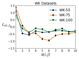
(b) Results on WK Datasets

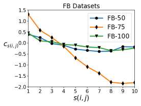
(c) Results on FB Datasets

Figure 4: Visualization of the $c_{s(i,j)}$ values learned by InGram with $B=10$. The $c_{s(i,j)}$ value is expected to be large for a small $s(i,j)$, and small for a large $s(i,j)$. See Section 5.1 for more details.

6.4 Ablation Studies of InGram

We conduct ablation studies for InGram to validate the importance of each module of InGram. Specifically, we compare the performance of InGram under the following settings: (i) we replace the attention-based aggregation in (1) and (LABEL:eq:nodeup) with the mean aggregator or (ii) the sum aggregator; (iii) when we update an entity representation in (LABEL:eq:nodeup), we replace $\bar{{\bf{z}}}_{i}^{(L)}$ with a separate learnable self-loop vector as in (Vashishth et al., 2020); (iv) we do not dynamically re-split $\mathcal{F}_{\text{tr}}$ and $\mathcal{T}_{\text{tr}}$ as described in Section 5.4, i.e., we fix the split during training; (v) we do not update a relation representation vector; (vi) we set $B=1$ in (3), i.e., we do not utilize the affinity weights in updating relation representations. The results of these settings are shown in Table 4 in order. Removing each module leads to a noticeable degradation in the performance of InGram. While some are more critical and others are less, InGram achieves the best performance when all modules come together.

6.5 Qualitative Analysis of InGram

In Section 5.1, when updating the relation vectors using (2), we introduce the learnable parameters $c_{s(i,j)}$ for computing the attention coefficient between $r_{i}$ and $r_{j}$. By definition of $s(i,j)$ in (3), the value of $s(i,j)$ is small if $r_{i}$ and $r_{j}$ are similar. Since we expect that two similar relations have a high attention value, we expect that $c_{s(i,j)}$ is large for a small $s(i,j)$, and $c_{s(i,j)}$ is small for a large $s(i,j)$. Figure 4 shows the learned $c_{s(i,j)}$ values according to $s(i,j)$. Even though some exceptions exist, overall, the plots are going down from left to right; the $c_{s(i,j)}$ values are learned as expected. Indeed, when we tune the number of bins $B\in\{1,5,10\}$, InGram achieves the best performance when $B=10$, showing the advantage of differentiating bins.

7 Conclusion and Future Work

We consider challenging and realistic inductive learning scenarios where new entities accompany new relations. Our method, InGram, can generate embeddings of new relations and entities only appearing at inference time. InGram conducts inferences based only on the structure of a given knowledge graph without any extra information about the entities and relations or the aid of rich language models.

While existing methods are biased toward learning the patterns of known relations, InGram focuses more on the generalization capability useful for modeling new relations. We will investigate the ways in which InGram can incorporate known-relation-specific patterns into inferences when known relations are dominant. We also plan to do the theoretical analysis of InGram as done in (Xu et al., 2019), (Barcelo et al., 2022) and (Hamilton et al., 2017), as well as consider some extensions to hyper-relational facts (Chung et al., 2023) and bi-level or hierarchical structures (Chung & Whang, 2023; Kwak et al., 2022). Finally, we will look into how we can make the predictions of InGram robust and reliable to possibly noisy information (Hong et al., 2023) in a given knowledge graph.

Appendix A Generating Datasets for Inductive Knowledge Graph Completion

Algorithm 2 Generating Datasets for Inductive Knowledge Graph Completion

Input: $\widetilde{G}=(\mathcal{V},\mathcal{R},\mathcal{E})$, $n_{\text{tr}}$, $n_{\text{inf}}$, $p_{\text{rel}}$, $p_{\text{tri}}$

Output: $\widetilde{G_{\text{tr}}}=(\mathcal{V}_{\text{tr}},\mathcal{R}_{\text{tr}},\mathcal{E}_{\text{tr}})$ and $\widetilde{G_{\text{inf}}}=(\mathcal{V}_{\text{inf}},\mathcal{R}_{\text{inf}},\mathcal{E}_{\text{inf}})$

1:  $\widetilde{G}\leftarrow$ Giant connected component of $\widetilde{G}$.

2:  Randomly split $\mathcal{R}$ into $\mathcal{R}_{\text{tr}}$ and $\mathcal{R}_{\text{inf}}$ such that $|\mathcal{R}_{\text{tr}}|:|\mathcal{R}_{\text{inf}}|=(1-p_{\text{rel}}):p_{\text{rel}}$.

3:  Uniformly sample $n_{\text{tr}}$ entities from $\mathcal{V}$ and form $\mathcal{V}_{\text{tr}}$ by taking the sampled entities and their two-hop neighbors. We select at most 50 neighbors per entity for each hop to prevent exponential growth.

4:  $\mathcal{E}_{\text{tr}}\coloneqq\{(v_{i},r,v_{j})|v_{i}\in\mathcal{V}_{\text{tr}},v_{j}\in\mathcal{V}_{\text{tr}},r\in\mathcal{R}_{\text{tr}},(v_{i},r,v_{j})\in\mathcal{E}\}$.

5:  $\mathcal{E}_{\text{tr}}\leftarrow$ Triplets in the giant connected component of $\mathcal{E}_{\text{tr}}$.

6:  $\mathcal{V}_{\text{tr}}\leftarrow$ Entities involved in $\mathcal{E}_{\text{tr}}$.

7:  $\mathcal{R}_{\text{tr}}\leftarrow$ Relations involved in $\mathcal{E}_{\text{tr}}$.

8:  Let $\widetilde{G}^{\prime}$ be the subgraph of $\widetilde{G}$ where the entities in $\mathcal{V}_{\text{tr}}$ are removed.

9:  In $\widetilde{G}^{\prime}$, uniformly sample $n_{\text{inf}}$ entities and form $\mathcal{V}_{\text{inf}}$ by taking the sampled entities and their two-hop neighbors. We select at most 50 neighbors per entity for each hop to prevent exponential growth.

10:  $\mathcal{E}_{\text{inf}}\coloneqq\mathcal{X}\cup\mathcal{Y}$ such that $|\mathcal{X}|:|\mathcal{Y}|=(1-p_{\text{tri}}):p_{\text{tri}}$ where $\mathcal{X}\coloneqq\{(v_{i},r,v_{j})|v_{i}\in\mathcal{V}_{\text{inf}},v_{j}\in\mathcal{V}_{\text{inf}},r\in\mathcal{R}_{\text{tr}},(v_{i},r,v_{j})\in\mathcal{E}\}$ and $\mathcal{Y}\coloneqq\{(v_{i},r,v_{j})|v_{i}\in\mathcal{V}_{\text{inf}},v_{j}\in\mathcal{V}_{\text{inf}},r\in\mathcal{R}_{\text{inf}},(v_{i},r,v_{j})\in\mathcal{E}\}$.

11:  $\mathcal{E}_{\text{inf}}\leftarrow$ Triplets in the giant connected component of $\mathcal{E}_{\text{inf}}$.

12:  $\mathcal{V}_{\text{inf}}\leftarrow$ Entities involved in $\mathcal{E}_{\text{inf}}$.

13:  $\mathcal{R}_{\text{inf}}\leftarrow$ Relations involved in $\mathcal{E}_{\text{inf}}$.

Algorithm 2 shows how we generate the datasets used in Section 6. Also, Table 5 and Table 6 show the statistic of the datasets and the hyperparameters used to create the datasets, respectively.

As described in Section 3, $\mathcal{E}_{\text{tr}}$ is divided into $\mathcal{F}_{\text{tr}}$ and $\mathcal{T}_{\text{tr}}$. How to split and use $\mathcal{E}_{\text{tr}}$ is a model-dependent design choice. On the other hand, $\mathcal{E}_{\text{inf}}$ is divided into three pairwise disjoint sets, $\mathcal{F}_{\text{inf}}$, $\mathcal{T}_{\text{val}}$, and $\mathcal{T}_{\text{test}}$ with a ratio of 3:1:1. For a fair comparison, these three sets are fixed, and the same sets are provided to each model.

In Section 4, we mentioned that we add reverse relations and triplets. While this addition is essential for GNN-based methods (Vashishth et al., 2020; Zhang & Yao, 2022), we should add the reverse relations and triplets after we split $\mathcal{F}_{\text{inf}}$, $\mathcal{T}_{\text{val}}$, and $\mathcal{T}_{\text{test}}$ to prevent data leakage problems. Similarly, we add the reverse relations and triplets after we split $\mathcal{F}_{\text{tr}}$ and $\mathcal{T}_{\text{tr}}$.

Appendix B Details about the Baseline Methods

All experiments were conducted with GeForce RTX 2080 Ti, GeForce RTX 3090 or RTX A6000, depending on the implementations of each method. We modified all the baseline models except RAILD and RMPI so that the models accept new relations since they do not consider new relations at inference time. We used the original implementations provided by the authors of the models with minimal modification (if needed) and used the default setting except for the things described below.

Since the original implementations of NeuralLP and DRUM include entities in $\mathcal{V}_{\text{tr}}$ as candidates for a prediction task at inference time, we excluded them from the candidates for a fair comparison. On the other hand, the implementations of BLP and RAILD restrict the candidates to be the entities involved in $\mathcal{T}_{\text{test}}$; so we modified this module to consider all entities in $\mathcal{V}_{\text{inf}}$ to be candidates.

BLP and QBLP require pre-trained vectors for entities and RAILD requires pre-trained vectors for both entities and relations, where the pre-trained vectors are produced by feeding text descriptions or names into BERT (Devlin et al., 2019). Among our datasets, NL does not have text descriptions, FB has text descriptions only for entities, and WK has text descriptions for both entities and relations. We provided the pre-trained vectors with BLP, QBLP and RAILD using the available information.

We tuned BLP with learning rate $\in\{0.00001,0.00002,0.00005\}$ and L2 regularization coefficient $\in\{0,0.001,0.01\}$. QBLP was tuned with learning rate $\in\{0.0001,0.0005\}$, the number of transformer layers $\in\{2,3,4\}$ and the number of GCN layers $\in\{2,3\}$. For GraIL, CoMPILE and SNRI, we set the early stop patience to be 10 validation trials and the number of total epochs to be 10. Following the original setting of RMPI, we used the Schema Enhanced RMPI for NL-25, NL-50, NL-75, and NL-100, and used the Randomly Initialized RMPI for NL-0 and NELL-995-v1. We tuned RED-GNN with weight decay $\in\{0.00001,0.01\}$, dropout rate $\in\{0,0.3\}$ and the number of layers $\in\{3,4\}$. We set the early stop patience to be 10 epochs.

Since the implementation of RAILD does not contain the codes for obtaining node2vec representations of relations, we used the official C++ implementation of node2vec to calculate the representations of relations.

The original implementation of CompGCN can only be applied to the transductive setting for both entities and relations. We modified CompGCN so that the model also uses randomly initialized embeddings for new entities appearing at inference time. CompGCN is tuned with the number of GCN layers $\in\{1,2,3\}$, learning rate $\in\{0.0001,0.001\}$ and the number of bases $\in\{-1,20,40\}$, where -1 denotes the case where each relation has its own embedding. We tuned NodePiece with the size of relational context $\in\{4,12\}$ and the margin $\in\{15,20,25\}$.

Missing Baselines.

We could not include PathCon (Wang et al., 2021) and TACT (Chen et al., 2021) in our experiments since their original source codes were written only for relation prediction but not for link prediction. ConGLR (Lin et al., 2022) and CBGNN (Yan et al., 2022) sample 50 negative candidates for each query, following the experimental setting of GraIL. Unlike GraIL, CoMPILE and SNRI, the original implementations of ConGLR and CBGNN do not provide the code for expanding the candidate set to $\mathcal{V}_{\text{inf}}$, so we could not include them as baseline methods. Since the entity sets of training and inference graphs are disjoint in our setting, we could not include baselines assuming new entities should be attached to known entities, such as MEAN (Hamaguchi et al., 2017) and LAN (Wang et al., 2019). We could not include GraphANGEL (Jin et al., 2022) in our experiments because the results in (Jin et al., 2022) are not reproducible.

Appendix C Hyperparameters of InGram

For InGram, we performed validation every 200 epochs for a total of 10,000 epochs. We tuned InGram with 10 negative samples, $d^{\prime}\in\{32,64,128,256\}$, $\widehat{d}^{\prime}\in\{128,256\}$, $L\in\{1,2,3\}$, $\widehat{L}\in\{2,3,4\}$, $K\in\{8,16\}$, $\widehat{K}\in\{8,16\}$, $\gamma\in\{1.0,1.5,2.0,2.5\}$, $B\in\{1,5,10\}$ and the learning rate $\in\{0.0005,0.001\}$. We observed that the best performance of InGram is achieved when $B=10$, showing the effectiveness of our binning strategy used in (3) described in Section 5.1.

Table 5: Datasets for Inductive Knowledge Graph Completion.

	NL-100			NL-75			NL-50			NL-25
	$|\mathcal{V}|$	$|\mathcal{R}|$	$|\mathcal{E}|$	$|\mathcal{V}|$	$|\mathcal{R}|$	$|\mathcal{E}|$	$|\mathcal{V}|$	$|\mathcal{R}|$	$|\mathcal{E}|$	$|\mathcal{V}|$	$|\mathcal{R}|$	$|\mathcal{E}|$
$\widetilde{G_{\text{tr}}}$	1,258	55	7,832	2,607	96	11,058	4,396	106	17,578	4,396	106	17,578
$\widetilde{G_{\text{inf}}}$	1,709	53	3,964	1,578	116	3,031	2,335	119	4,294	2,146	120	3,717
	WK-100			WK-75			WK-50			WK-25
	$|\mathcal{V}|$	$|\mathcal{R}|$	$|\mathcal{E}|$	$|\mathcal{V}|$	$|\mathcal{R}|$	$|\mathcal{E}|$	$|\mathcal{V}|$	$|\mathcal{R}|$	$|\mathcal{E}|$	$|\mathcal{V}|$	$|\mathcal{R}|$	$|\mathcal{E}|$
$\widetilde{G_{\text{tr}}}$	9,784	67	49,875	6,853	52	28,741	12,022	72	82,481	12,659	47	41,873
$\widetilde{G_{\text{inf}}}$	12,136	37	22,479	2,722	65	5,717	9,328	93	16,121	3,228	74	5,652
	FB-100			FB-75			FB-50			FB-25
	$|\mathcal{V}|$	$|\mathcal{R}|$	$|\mathcal{E}|$	$|\mathcal{V}|$	$|\mathcal{R}|$	$|\mathcal{E}|$	$|\mathcal{V}|$	$|\mathcal{R}|$	$|\mathcal{E}|$	$|\mathcal{V}|$	$|\mathcal{R}|$	$|\mathcal{E}|$
$\widetilde{G_{\text{tr}}}$	4,659	134	62,809	4,659	134	62,809	5,190	153	85,375	5,190	163	91,571
$\widetilde{G_{\text{inf}}}$	2,624	77	11,645	2,792	186	15,528	4,445	205	19,394	4,097	216	28,579

Table 6: Hyperparameters Used to Create the Datasets.

	NL-100	NL-75	NL-50	NL-25	NL-0	WK-100	WK-75	WK-50	WK-25	FB-100	FB-75	FB-50	FB-25
$n_{\text{tr}}$	15	60	50	50	20	20	20	30	30	10	10	10	10
$n_{\text{inf}}$	80	50	80	80	80	250	15	80	50	20	20	50	50
$p_{\text{rel}}$	0.40	0.40	0.40	0.40	0.00	0.30	0.40	0.30	0.50	0.40	0.40	0.30	0.25
$p_{\text{tri}}$	1.00	0.75	0.50	0.25	0.00	1.00	0.75	0.50	0.25	1.00	0.75	0.50	0.25

References

- Abboud et al. (2021) Abboud, R., Ceylan, İ. İ., Grohe, M., and Lukasiewicz, T. The surprising power of graph neural networks with random node initialization. In Proceedings of the 30th International Joint Conference on Artificial Intelligence, pp. 2112–2118, 2021.
- Ali et al. (2021) Ali, M., Berrendorf, M., Galkin, M., Thost, V., Ma, T., Tresp, V., and Lehmann, J. Improving inductive link prediction using hyper-relational facts. In Proceedings of the 20th International Semantic Web Conference, pp. 74–92, 2021.
- Barcelo et al. (2022) Barcelo, P., Galkin, M., Morris, C., and Orth, M. R. Weisfeiler and Leman go relational. In Proceedings of the 1st Learning on Graphs Conference, 2022.
- Brody et al. (2022) Brody, S., Alon, U., and Yahav, E. How attentive are graph attention networks? In Proceedings of the 10th International Conference on Learning Representations, 2022.
- Chen et al. (2021) Chen, J., He, H., Wu, F., and Wang, J. Topology-aware correlations between relations for inductive link prediction in knowledge graphs. In Proceedings of the 35th AAAI Conference on Artificial Intelligence, pp. 6271–6278, 2021.
- Chung & Whang (2023) Chung, C. and Whang, J. J. Learning representations of bi-level knowledge graphs for reasoning beyond link prediction. In Proceedings of the 37th AAAI Conference on Artificial Intelligence, pp. 4208–4216, 2023.
- Chung et al. (2023) Chung, C., Lee, J., and Whang, J. J. Representation learning on hyper-relational and numeric knowledge graphs with transformers. In Proceedings of the 29th ACM SIGKDD Conference on Knowledge Discovery and Data Mining, pp. 310–322, 2023.
- Cui et al. (2022) Cui, Y., Wang, Y., Sun, Z., Liu, W., Jiang, Y., Han, K., and Hu, W. Inductive knowledge graph reasoning for multi-batch emerging entities. In Proceedings of the 31st ACM International Conference on Information and Knowledge Management, pp. 335–344, 2022.
- Dai et al. (2021) Dai, D., Zheng, H., Luo, F., Yang, P., Liu, T., Sui, Z., and Chang, B. Inductively representing out-of-knowledge-graph entities by optimal estimation under translational assumptions. In Proceedings of the 6th Workshop on Representation Learning for NLP, pp. 83–89, 2021.
- Daza et al. (2021) Daza, D., Cochez, M., and Groth, P. Inductive entity representations from text via link prediction. In Proceedings of the Web Conference 2021, pp. 798–808, 2021.
- Devlin et al. (2019) Devlin, J., Chang, M.-W., Lee, K., and Toutanova, K. BERT: Pre-training of deep bidirectional transformers for language understanding. In Proceedings of the 2019 Conference of the North American Chapter of the Association for Computational Linguistics: Human Language Technologies, pp. 4171–4186, 2019.
- Galkin et al. (2022) Galkin, M., Denis, E., Wu, J., and Hamilton, W. L. NodePiece: Compositional and parameter-efficient representations of large knowledge graphs. In Proceedings of the 10th International Conference on Learning Representations, 2022.
- Geng et al. (2023) Geng, Y., Chen, J., Pan, J. Z., Chen, M., Jiang, S., Zhang, W., and Chen, H. Relational message passing for fully inductive knowledge graph completion. In Proceedings of the 39th IEEE International Conference on Data Engineering, 2023.
- Gesese et al. (2022) Gesese, G. A., Sack, H., and Alam, M. RAILD: Towards leveraging relation features for inductive link prediction in knowledge graphs. In Proceedings of the 11th International Joint Conference on Knowledge Graphs, 2022.
- Glorot & Bengio (2010) Glorot, X. and Bengio, Y. Understanding the difficulty of training deep feedforward neural networks. In Proceedings of the 13th International Conference on Artificial Intelligence and Statistics, pp. 249–256, 2010.
- Hamaguchi et al. (2017) Hamaguchi, T., Oiwa, H., Shimbo, M., and Matsumoto, Y. Knowledge transfer for out-of-knowledge-base entities: A graph neural network approach. In Proceedings of the 26th International Joint Conference on Artificial Intelligence, pp. 1802–1808, 2017.
- Hamilton et al. (2017) Hamilton, W. L., Ying, R., and Leskovec, J. Inductive representation learning on large graphs. In Proceedings of the 31st Conference on Neural Information Processing System, pp. 1025–1035, 2017.
- He et al. (2016) He, K., Zhang, X., Ren, S., and Sun, J. Deep residual learning for image recognition. In 2016 IEEE Conference on Computer Vision and Pattern Recognition, pp. 770–778, 2016.
- Hong et al. (2023) Hong, G., Kim, J., Kang, J., Myaeng, S.-H., and Whang, J. J. Discern and answer: Mitigating the impact of misinformation in retrieval-augmented models with discriminators. arXiv preprint arXiv:2305.01579, 2023. doi: 10.48550/arXiv.2305.01579.
- Ji et al. (2022) Ji, S., Pan, S., Cambria, E., Marttinen, P., and Yu, P. S. A survey on knowledge graphs: Representation, acquisition, and applications. IEEE Transactions on Neural Networks and Learning Systems, 33(2):494–514, 2022.
- Jin et al. (2022) Jin, J., Wang, Y., Du, K., Zhang, W., Zhang, Z., Wipf, D., Yu, Y., and Gan, Q. Inductive relation prediction using analogy subgraph embeddings. In Proceedings of the 10th International Conference on Learning Representations, 2022.
- Kipf & Welling (2017) Kipf, T. N. and Welling, M. Semi-supervised classification with graph convolutional networks. In Proceedings of the 5th International Conference on Learning Representations, 2017.
- Kwak et al. (2022) Kwak, J. H., Lee, J., Whang, J. J., and Jo, S. Semantic grasping via a knowledge graph of robotic manipulation: A graph representation learning approach. IEEE Robotics and Automation Letters, 7(4):9397–9404, 2022.
- Lin et al. (2022) Lin, Q., Liu, J., Xu, F., Pan, Y., Zhu, Y., Zhang, L., and Zhao, T. Incorporating context graph with logical reasoning for inductive relation prediction. In Proceedings of the 45th International ACM SIGIR Conference on Research and Development in Information Retrieval, pp. 893–903, 2022.
- Liu et al. (2017) Liu, H., Wu, Y., and Yang, Y. Analogical inference for multi-relational embeddings. In Proceedings of the 37th International Conference on Machine Learning, pp. 2168–2178, 2017.
- Liu et al. (2021) Liu, S., Grau, B., Horrocks, I., and Kostylev, E. INDIGO: GNN-based inductive knowledge graph completion using pair-wise encoding. In Proceedings of the 35th Conference on Neural Information Processing Systems, pp. 2034–2045, 2021.
- Maas et al. (2013) Maas, A. L., Hannun, A. Y., and Ng, A. Y. Rectifier nonlinearities improve neural network acoustic models. In ICML 2013 Workshop on Deep Learning for Audio, Speech and Language Processing, 2013.
- Mai et al. (2021) Mai, S., Zheng, S., Yang, Y., and Hu, H. Communicative message passing for inductive relation reasoning. In Proceedings of the 35th AAAI Conference on Artificial Intelligence, pp. 4294–4302, 2021.
- Markowitz et al. (2022) Markowitz, E., Balasubramanian, K., Mirtaheri, M., Annavaram, M., Galstyan, A., and Steeg, G. V. StATIK: Structure and text for inductive knowledge graph completion. In Findings of the Association for Computational Linguistics: NAACL 2022, pp. 604–615, 2022.
- Nathani et al. (2019) Nathani, D., Chauhan, J., Sharma, C., and Kaul, M. Learning attention-based embeddings for relation prediction in knowledge graphs. In Proceedings of the 57th Annual Meeting of the Association for Computational Linguistics, pp. 4710–4723, 2019.
- Sadeghian et al. (2019) Sadeghian, A., Armandpour, M., patrick Ding, and Wang, D. Z. DRUM: End-to-end differentiable rule mining on knowledge graphs. In Proceedings of the 33rd Conference on Neural Information Processing Systems, pp. 15347–15357, 2019.
- Sato et al. (2021) Sato, R., Yamada, M., and Kashima, H. Random features strengthen graph neural networks. In Proceedings of the 2021 SIAM International Conference on Data Mining, pp. 333–341, 2021.
- Schlichtkrull et al. (2018) Schlichtkrull, M., Kipf, T. N., Bloem, P., van den Berg, R., Titov, I., and Welling, M. Modeling relational data with graph convolutional networks. In Proceedings of the 15th International Semantic Web Conference, pp. 593–607, 2018.
- Sun et al. (2019) Sun, Z., Deng, Z.-H., Nie, J.-Y., and Tang, J. RotatE: Knowledge graph embedding by relational rotation in complex space. In Proceedings of the 7th International Conference on Learning Representations, 2019.
- Teru et al. (2020) Teru, K., Denis, E., and Hamilton, W. Inductive relation prediction by subgraph reasoning. In Proceedings of the 37th International Conference on Machine Learning, pp. 9448–9457, 2020.
- Toutanova & Chen (2015) Toutanova, K. and Chen, D. Observed versus latent features for knowledge base and text inference. In Proceedings of the 3rd Workshop on Continuous Vector Space Models and their Compositionality, pp. 57–66, 2015.
- Vashishth et al. (2020) Vashishth, S., Sanyal, S., Nitin, V., and Talukdar, P. Composition-based multi-relational graph convolutional networks. In Proceedings of the 8th International Conference on Learning Representations, 2020.
- Vaswani et al. (2017) Vaswani, A., Shazeer, N., Parmar, N., Uszkoreit, J., Jones, L., Gomez, A. N., Łukasz Kaiser, and Polosukhin, I. Attention is all you need. In Proceedings of the 31st Conference on Neural Information Processing Systems, pp. 5998–6008, 2017.
- Veličković et al. (2018) Veličković, P., Cucurull, G., Casanova, A., Romero, A., Liò, P., and Bengio, Y. Graph attention networks. In Proceedings of the 6th International Conference on Learning Representations, 2018.
- Wang et al. (2022) Wang, C., Zhou, X., Pan, S., Dong, L., Song, Z., and Sha, Y. Exploring relational semantics for inductive knowledge graph completion. In Proceedings of the 36th AAAI Conference on Artificial Intelligence, pp. 4184–4192, 2022.
- Wang et al. (2021) Wang, H., Ren, H., and Leskovec, J. Relational message passing for knowledge graph completion. In Proceedings of the 27th ACM SIGKDD Conference on Knowledge Discovery and Data Mining, pp. 1697–1707, 2021.
- Wang et al. (2019) Wang, P., Han, J., Li, C., and Pan, R. Logic attention based neighborhood aggregation for inductive knowledge graph embedding. In Proceedings of the 33rd AAAI Conference on Artificial Intelligence, pp. 7152–7159, 2019.
- Wang et al. (2017) Wang, Q., Mao, Z., Wang, B., and Guo, L. Knowledge graph embedding: A survey of approaches and applications. IEEE Transactions on Knowledge and Data Engineering, 29(12):2724–2743, 2017.
- Xiong et al. (2017) Xiong, W., Hoang, T., and Wang, W. Y. DeepPath: A reinforcement learning method for knowledge graph reasoning. In Proceedings of the 2017 Conference on Empirical Methods in Natural Language Processing, pp. 564–573, 2017.
- Xu et al. (2019) Xu, K., Hu, W., Leskovec, J., and Jegelka, S. How powerful are graph neural networks? In Proceedings of the 7th International Conference on Learning Representations, 2019.
- Xu et al. (2022) Xu, X., Zhang, P., He, Y., Chao, C., and Yan, C. Subgraph neighboring relations infomax for inductive link prediction on knowledge graphs. In Proceedings of the 31st International Joint Conference on Artificial Intelligence, pp. 2341–2347, 2022.
- Yan et al. (2022) Yan, Z., Ma, T., Gao, L., Tang, Z., and Chen, C. Cycle representation learning for inductive relation prediction. In Proceedings of the 39th International Conference on Machine Learning, pp. 24895–24910, 2022.
- Yang et al. (2015) Yang, B., tau Yih, W., He, X., Gao, J., and Deng, L. Embedding entities and relations for learning and inference in knowledge bases. In Proceedings of the 3rd International Conference on Learning Representations, 2015.
- Yang et al. (2017) Yang, F., Yang, Z., and Cohen, W. W. Differentiable learning of logical rules for knowledge base reasoning. In Proceedings of the 31st Conference on Neural Information Processing Systems, pp. 2319–2328, 2017.
- Ying et al. (2021) Ying, C., Cai, T., Luo, S., Zheng, S., Ke, G., He, D., Shen, Y., and Liu, T.-Y. Do transformers really perform badly for graph representation? In Proceedings of the 35th Conference on Neural Information Processing Systems, pp. 28877–28888, 2021.
- Zha et al. (2022) Zha, H., Chen, Z., and Yan, X. Inductive relation prediction by BERT. In Proceedings of the 36th AAAI Conference on Artificial Intelligence, pp. 5923–5931, 2022.
- Zhang & Yao (2022) Zhang, Y. and Yao, Q. Knowledge graph reasoning with relational digraph. In Proceedings of the ACM Web Conference 2022, pp. 912–924, 2022.
- Zhu et al. (2021) Zhu, Z., Zhang, Z., Xhonneux, L.-P., and Tang, J. Neural Bellman-Ford networks: A general graph neural network framework for link prediction. In Proceedings of the 35th Conference on Neural Information Processing System, pp. 29476–29490, 2021.