Primordial Non-Gaussianity $f_{\mathrm{NL}}$ and Anisotropies in Scalar-Induced Gravitational Waves

Abstract

Primordial non-Gaussianity encodes vital information of the physics of the early universe, particularly during the inflationary epoch. To explore the local-type primordial non-Gaussianity $f_{\mathrm{NL}}$, we study the anisotropies in gravitational wave background induced by the linear cosmological scalar perturbations during radiation domination in the early universe. We provide the first complete analysis to the angular power spectrum of such scalar-induced gravitational waves. The spectrum is expressed in terms of the initial inhomogeneities, the Sachs-Wolfe effect, and their crossing. It is anticipated to have frequency dependence and multipole dependence, i.e., $C_{\ell}(\nu)\propto[\ell(\ell+1)]^{-1}$ with $\nu$ being a frequency and $\ell$ referring to the $\ell$-th spherical harmonic multipole. In particular, the initial inhomogeneites in this background depend on gravitational-wave frequency. These properties are potentially useful for the component separation, foreground removal, and breaking degeneracies in model parameters, making the non-Gaussian parameter $f_{\mathrm{NL}}$ measurable. Further, theoretical expectations may be tested by space-borne gravitational-wave detectors in future.

1 Introduction

The PNG refers to deviations from Gaussian statistics in the linear cosmological perturbations originated from quantum fluctuations during the inflationary epoch of the early universe [1, 2, 3, 4, 5, 6, 7]. A quantity of mechanisms related to the generation of PNG have been proposed (see Ref. [8] for reviews), for example, nonlinear couplings between the inflaton and other fields [9, 10, 11, 12, 13, 14, 15, 16, 17], non-standard inflation models [18, 19, 20, 21, 22, 23, 24, 25, 26], and so on. The primordial non-Gaussian parameter $f_{\mathrm{NL}}$ represents a higher or lower probability of large overdensities, depending on its sign. Therefore, the study of PNG is not only important for understanding the underlying physics of the early universe, but also the formation and evolution of cosmic structures.

There are several observational constraints on the PNG, but they are limited to cosmological curvature perturbations on large scales comparable to the whole scale of the observable universe. Via measurements of anisotropies and polarization in the CMB, the Planck collaboration [27] has reported highly Gaussian curvature perturbations that are compatible with anticipations of canonical single-field slow-roll inflation [28]. Constraints have also been provided via measurements of CMB spectral distortions [29, 30], galaxy formation [31], and UV luminosity function [32], etc., but all of them are less precise than the Planck results. We should note that the above measurements are only sensitive to the large-scale curvature perturbations, which are related to the dynamics of inflation during the 50-60 e-foldings before its end.

Detection of GW can provide a new observational window to the nature of cosmological curvature perturbations on smaller scales, which were generated during later stages of inflation. It is well known that only the physics imprinted on the last-scattering surface of CMB can be measured, due to the tightly coupled limit before the free streaming of photons [33]. In contrast, the GW probe overcomes such a defect and thereby has potentials to directly measure the physics playing significant roles on more remote distances [34, 35, 36, 37, 38, 39, 40, 41, 42, 43], which are corresponded to higher redshifts, because GW propagate almost freely after production [44, 45]. Smaller-scale modes exited the Hubble horizon later during inflation, but reentered the Hubble horizon at higher redshifts after the end of inflation. Therefore, we expect the GW probe to be sensitive to the primordial non-Gaussianity of small-scale perturbations and thereby the dynamics of inflation at the late stage.

After reentering into the Hubble horizon, the small-scale curvature perturbations nonlinearly produced a CGWB, and the PNG left significant imprints on the background [46, 47, 48, 49, 50, 51, 52, 53, 54], making the background to be a potential probe to the PNG. Conventionally, such a CGWB is also called the SIGW [55, 56, 57, 58, 59, 60], since it was induced at second order by the linear scalar perturbations in the early universe. Depending on values of the local-type non-Gaussian parameter $f_{\mathrm{NL}}$, the contribution of PNG to the energy-density fraction spectrum of SIGW could be two orders of magnitude larger than the Gaussian contribution, as was shown in Ref. [53]. If the perturbativity conditions are required during inflation, some viable models have been considered in Ref. [54], where the authors studied SIGW in the Starobinsky’s model with a dip [61, 62] and the model of critical-Higgs inflation [63, 64, 65]. For simplicity, we would not be concerned with such concrete scenarios in our current work. Recently, a common-spectrum process reported by the NANOGrav collaboration [66] was speculated to be evidence for SIGW in the literature [67, 68, 69, 70, 71, 72, 73, 74, 75], though not confirmed until now .

Besides the vital contribution to SIGW, the PNG also impacts the formation of PBH and particularly alters the mass distribution function of PBH [80, 81, 82, 83, 26, 84, 61, 85, 86, 87, 88]. Since PBH could be formed due to gravitational collapse of enhanced small-scale curvature perturbations [89] and the PDF of the latter is deformed by the PNG, the abundance of PBH would be significantly enhanced or suppressed compared with results for the Gaussian perturbations, depending on the sign of the non-Gaussian parameter (e.g., see Refs. [81, 82]). On the other hand, in the early universe, SIGW were also produced as an accompaniment to the production of PBH, making SIGW a potential probe to PBH [90, 91, 92, 93] and then the PNG correspondingly.

In summary, the study of SIGW is important for determination of the PNG. The energy-density fraction spectrum of SIGW has been used for this aim in the literature [48, 49, 50, 51, 52, 53, 54]. However, we will show that such a spectrum, i.e., the monopole, has a sign degeneracy in the non-Gaussian parameter. We will further show that there are degeneracies in the non-Gaussian parameter and other model parameters, indicating that the non-Gaussian contribution can be mimicked by these parameters. In addition, other gravitational-wave backgrounds originating from astrophysical processes would be foregrounds that may contaminate the signal (see Ref. [94] and references therein). Due to the above reasons, it is particularly challenging to measure the PNG with the monopole in SIGW. Therefore, it is necessary to develop some new probes.

In this work, we propose that the anisotropies in SIGW could be a powerful probe to the local-type PNG on scales that can not be probed otherwise (e.g., via CMB). We will provide the complete analysis to the angular power spectrum of SIGW for the first time. We will also show its frequency dependence and multipole dependence, which could be useful for breaking the aforementioned degeneracies of model parameters and the foreground removal as well as component separation [95]. Before our present work, the line-of-sight method for the study of anisotropies in a GW background has been developed in Ref. [96], analogue to that for the study of anisotropies and polarization in CMB [97]. Subsequently, it was adopted to study the anisotropies and non-Gaussianity in CGWB in Refs. [98, 99]. Assuming the local-type PNG upon the squeezed limit, the anisotropies in SIGW as well as implications of them for PBH were studied for the first time in Ref. [100]. However, such a study is incomplete, as will be demonstrated in our present work. Following Ref. [100], other related works can be found in Refs. [101, 102, 103, 94, 104, 105, 106, 107].One of the leading aims of our present work is to establish the first complete analysis.

The remaining context of this paper is arranged as follows. In Section 2, we will briefly review formulae of the inhomogeneous energy density of gravitational waves as well as the Boltzmann equation for the distribution function of gravitons. In Section 3, we will summarize the generic theory of SIGW. In Section 4, we reproduce the theoretical results of the monopole in SIGW, and show the degeneracies in model parameters. In Section 5, we provide the complete analysis of multipoles in SIGW, including the formulae of angular power spectrum and its properties. In Section 6, we make concluding remarks.

2 Basics of cosmological gravitational wave background

We consider a spatially-flat FRW metric in the conformal Newtonian gauge, with perturbations characterized by the linear scalar perturbations $\Phi(\eta,\mathbf{x})$ and $\Psi(\eta,\mathbf{x})$, and the transverse-traceless tensor perturbations $\chi_{ij}(\eta,\mathbf{x})$, i.e., the GW. We disregard the vector perturbations due to inflation. The perturbed metric is given by

$$\mathrm{d}s^{2}=a^{2}\left\{-(1+2\Phi)\mathrm{d}\eta^{2}+\left[(1-2\Psi)\delta_{ij}+\chi_{ij}\right]\mathrm{d}x^{i}\mathrm{d}x^{j}\right\}\ ,$$ (2.1)

where $a(\eta)$ is the scale factor of the universe at conformal time $\eta$. It is convenient to expand $\Phi(\eta,\mathbf{x})$ (we expand $\Psi(\eta,\mathbf{x})$ in the same way) and $\chi_{ij}(\eta,\mathbf{x})$ in Fourier space, i.e.,

$$\Phi(\eta,\mathbf{x}) = \int\frac{\mathrm{d}^{3}\mathbf{q}}{(2\pi)^{3/2}}e^{i\mathbf{q}\cdot\mathbf{x}}\Phi(\eta,\mathbf{q})\ ,$$ (2.2)

$$\chi_{ij}(\eta,\mathbf{x}) = \sum_{\lambda=+,\times}\int\frac{\mathrm{d}^{3}\mathbf{q}}{(2\pi)^{3/2}}e^{i\mathbf{q}\cdot\mathbf{x}}\epsilon_{ij}^{\lambda}(\mathbf{q})\chi_{\lambda}(\eta,\mathbf{q})\ ,$$ (2.3)

where we define two polarization tensors $\epsilon^{+}_{ij}(\mathbf{q})=\left[\epsilon_{i}(\mathbf{q})\epsilon_{j}(\mathbf{q})-\bar{\epsilon}_{i}(\mathbf{q})\bar{\epsilon}_{j}(\mathbf{q})\right]/\sqrt{2}$ and $\epsilon^{\times}_{ij}(\mathbf{q})=\left[\epsilon_{i}(\mathbf{q})\bar{\epsilon}_{j}(\mathbf{q})+\bar{\epsilon}_{i}(\mathbf{q})\epsilon_{j}(\mathbf{q})\right]/\sqrt{2}$, with $\epsilon_{i}(\mathbf{q})$ and $\bar{\epsilon}_{i}(\mathbf{q})$ being a set of orthonormal basis which is perpendicular to the wavevector $\mathbf{q}$. We further define the power spectrum of GW as the two-point correlator of $\chi_{\lambda}$, i.e.,

$$\langle\chi_{\lambda}(\eta,\mathbf{q})\chi_{\lambda^{\prime}}(\eta,\mathbf{q}^{\prime})\rangle=\delta_{\lambda\lambda^{\prime}}\delta^{(3)}(\mathbf{q}+\mathbf{q}^{\prime})P_{\chi_{\lambda}}(\eta,q)\ ,$$ (2.4)

which characterizes the statistical property. In the following, we will introduce several useful definitions and conventions of CGWB, as well as the Boltzmann equation of gravitons. In fact, most of them are analogue to those for CMB [97], and we would follow Refs. [96, 98, 99].

2.1 Energy density with inhomogeneities

At a conformal time $\eta$ and spatial location $\mathbf{x}$, the energy density of GW on subhorizon scales is defined as [34]

$$\rho_{\mathrm{gw}}(\eta,\mathbf{x})=\frac{m_{\mathrm{Pl}}^{2}}{4a^{2}(\eta)}\mkern 1.5mu\overline{\mkern-1.5mu\partial_{l}\chi_{ij}(\eta,\mathbf{x})\partial_{l}\chi_{ij}(\eta,\mathbf{x})\mkern-1.5mu}\mkern 1.5mu\ ,$$ (2.5)

where the overbar denotes a time average over oscillations, and $m_{\mathrm{Pl}}=({8\pi G})^{-1/2}$ is the Planck mass. Throughout this paper, we use $\partial_{\eta}$ and $\partial_{i}$ to denote $\partial/\partial\eta$ and $\partial/\partial x^{i}$, respectively. The energy density spectrum $\Omega_{\mathrm{gw}}(\eta,\mathbf{x},q)$ is defined as [34]

$$\rho_{\mathrm{gw}}(\eta,\mathbf{x})=\rho_{\mathrm{c}}\int\mathrm{d}\ln q\,\Omega_{\mathrm{gw}}(\eta,\mathbf{x},q)\ ,$$ (2.6)

with the critical energy density of the universe defined in terms of the conformal Hubble parameter $\mathcal{H}(\eta)={\partial_{\eta}{a}}/{a}$ as $\rho_{\mathrm{c}}=3m_{\mathrm{Pl}}^{2}\mathcal{H}^{2}/a^{2}$. We further introduce the energy-density full spectrum $\omega_{\mathrm{gw}}(\eta,\mathbf{x},\mathbf{q})$, which is direction-dependent, as

$$\Omega_{\mathrm{gw}}(\eta,\mathbf{x},q)=\int\mathrm{d}^{2}\mathbf{n}\,\omega_{\mathrm{gw}}(\eta,\mathbf{x},\mathbf{q})\ ,$$ (2.7)

where $\mathbf{q}$ denotes the comoving momentum of GWs and $\mathbf{n}$ denotes the propagation direction of GWs, i.e., $\mathbf{q}=q\mathbf{n}$ with $q=|\mathbf{q}|$. Therefore, we get an explicit expression of it to be

$$\omega_{\mathrm{gw}}(\eta,\mathbf{x},\mathbf{q})=-\frac{q^{3}}{12\mathcal{H}^{2}}\int\frac{\mathrm{d}^{3}\mathbf{k}}{(2\pi)^{3}}e^{i\mathbf{k}\cdot\mathbf{x}}\left(\mathbf{k}-\mathbf{q}\right)\cdot\mathbf{q}\sum_{\lambda,\lambda^{\prime}}\epsilon_{ij}^{\lambda}(\mathbf{k}-\mathbf{q})\epsilon_{ij}^{\lambda^{\prime}}(\mathbf{q})\mkern 1.5mu\overline{\mkern-1.5mu\chi_{\lambda}(\eta,\mathbf{k}-\mathbf{q})\chi_{\lambda^{\prime}}(\eta,\mathbf{q})\mkern-1.5mu}\mkern 1.5mu\ .$$ (2.8)

It is crucial to note that $\mathbf{k}$ is associated with the Fourier modes of overdensities in CGWB.

The full spectrum $\omega_{\mathrm{gw}}(\eta,\mathbf{x},\mathbf{q})$ can be decomposed into a homogeneous and isotropic background $\bar{\omega}_{\mathrm{gw}}(\eta,q)$ and superimposed fluctuations $\delta\omega_{\mathrm{gw}}(\eta,\mathbf{x},\mathbf{q})$.

The former is also called the monopole. It can be obtained from the definition of $\omega_{\mathrm{gw}}(\eta,\mathbf{x},\mathbf{q})$ in Eq. 2.7, i.e.,

$$\bar{\omega}_{\mathrm{gw}}(\eta,q)=\frac{\bar{\Omega}_{\mathrm{gw}}(\eta,q)}{4\pi}\ .$$ (2.9)

Here, $\bar{\Omega}_{\mathrm{gw}}(\eta,q)$ stands for the energy-density fraction spectrum defined by the spatial average of $\Omega_{\mathrm{gw}}(\eta,\mathbf{x},q)$ as follows [108]

$$\bar{\Omega}_{\mathrm{gw}}(\eta,q)=\left\langle\Omega_{\mathrm{gw}}(\eta,\mathbf{x},q)\right\rangle_{\mathbf{x}}=\frac{q^{5}}{24\pi^{2}\mathcal{H}^{2}}\sum_{\lambda=+,\times}\mkern 1.5mu\overline{\mkern-1.5muP_{\chi_{\lambda}}(\eta,q)\mkern-1.5mu}\mkern 1.5mu\ ,$$ (2.10)

where the angle brackets with a suffix _x denote the spatial average that is equivalent to the ensemble average. Besides Eq. 2.7, we also have used Eq. 2.4 and Eq. 2.8 during the derivation process of Eq. 2.10.

The inhomogeneities $\delta\omega_{\mathrm{gw}}$ on top of the background, leading to the multipoles in a CGWB discussed in the following, can be written as

$$\delta\omega_{\mathrm{gw}}(\eta,\mathbf{x},\mathbf{q})=\omega_{\mathrm{gw}}(\eta,\mathbf{x},\mathbf{q})-\bar{\omega}_{\mathrm{gw}}(\eta,q)\ ,$$ (2.11)

which can be recast to be the density contrast of the form

$$\delta_{\mathrm{gw}}(\eta,\mathbf{x},\mathbf{q})=\frac{\delta\omega_{\mathrm{gw}}(\eta,\mathbf{x},\mathbf{q})}{\bar{\omega}_{\mathrm{gw}}(\eta,q)}=4\pi\frac{\delta\omega_{\mathrm{gw}}(\eta,\mathbf{x},\mathbf{q})}{\bar{\Omega}_{\mathrm{gw}}(\eta,q)}\ .$$ (2.12)

To study the statistics of the fluctuations, we use the two-point correlation of $\delta_{\mathrm{gw}}(\eta,\mathbf{x},\mathbf{q})$. It is useful to expand $\delta_{\mathrm{gw}}$ in spherical harmonics along the direction $\mathbf{n}$, i.e.,

$$\delta_{\mathrm{gw}}(\eta,\mathbf{x},\mathbf{q})=\sum_{\ell}\sum_{m=-\ell}^{\ell}\delta_{\mathrm{gw},\ell m}(\eta,\mathbf{x},q)Y_{\ell m}(\mathbf{n})\ ,$$ (2.13)

where we have used the relation $\mathbf{q}=q\mathbf{n}$, and the multipole coefficients are given by

$$\delta_{\mathrm{gw},\ell m}(\eta,\mathbf{x},q)=\int\mathrm{d}^{2}\mathbf{n}\,Y_{\ell m}^{\ast}(\mathbf{n})\delta_{\mathrm{gw}}(\eta,\mathbf{x},\mathbf{q})\ .$$ (2.14)

Assuming the statistical isotropy on large scales, we define the reduced angular power spectrum as a two-point correlator of the multipole coefficients $\delta_{\mathrm{gw},\ell m}(\eta_{0},\mathbf{x}_{0},q)$, with the observing time and location $(\eta_{0},\mathbf{x}_{0})$ omitted for brevity hereafter, i.e.,

$$\langle\delta_{\mathrm{gw},\ell m}(q)\delta_{\mathrm{gw},\ell^{\prime}m^{\prime}}^{\ast}(q^{\prime})\rangle=\delta_{\ell\ell^{\prime}}\delta_{mm^{\prime}}\widetilde{C}_{\ell}(q,q^{\prime})\ ,$$ (2.15)

where the tilde stands for a reduced quantity. In fact, this is cross-correlation at two frequency bands denoted by $q$ and $q^{\prime}$. Further, the angular power spectrum is defined as the two-point correlator of $\delta\omega_{\mathrm{gw}}(q)$, i.e.,

$$\left\langle\delta\omega_{\mathrm{gw},\ell m}(q)\delta\omega_{\mathrm{gw},\ell^{\prime}m^{\prime}}^{\ast}(q^{\prime})\right\rangle=\delta_{\ell\ell^{\prime}}\delta_{mm^{\prime}}C_{\ell}(q,q^{\prime})\ .$$ (2.16)

A relation between $\widetilde{C}_{\ell}$ and $C_{\ell}$ can be derived from Eq. 2.12, namely,

$$\widetilde{C}_{\ell}(q,q^{\prime})=\frac{(4\pi)^{2}C_{\ell}(q,q^{\prime})}{\bar{\Omega}_{\mathrm{gw}}(q)\bar{\Omega}_{\mathrm{gw}}(q^{\prime})}\ ,$$ (2.17)

where $\bar{\Omega}_{\mathrm{gw}}(q)$ denotes the energy-density fraction spectrum in the observer frame with $(\eta_{0},\mathbf{x}_{0})$. Here, besides correlations between the same frequency band (i.e., $q=q^{\prime}$), we also consider correlations between different frequency bands (i.e., $q\neq q^{\prime}$). Such a consideration would give rise to non-trivial theoretical results, as will be shown in Section 5.2.

2.2 Boltzmann equation

Following Refs. [96, 98, 99], we review the Boltzmann equation for gravitons in general. The energy density in Eq. 2.5 is expressed in terms of the distribution function of gravitons $f(\eta,\mathbf{x},\mathbf{q})$, i.e.,

$$\rho_{\mathrm{gw}}(\eta,\mathbf{x})=\frac{1}{a^{4}}\int\mathrm{d}^{3}\mathbf{q}\,qf(\eta,\mathbf{x},\mathbf{q})\ .$$ (2.18)

Combining it with Eq. 2.6 and Eq. 2.7, we obtain a relation of the form

$$f(\eta,\mathbf{x},\mathbf{q})=\rho_{\mathrm{c}}\left(\frac{a}{q}\right)^{4}\omega_{\mathrm{gw}}(\eta,\mathbf{x},\mathbf{q})\ .$$ (2.19)

Analogue to decomposition of $\omega_{\mathrm{gw}}$ in Section 2.1, the distribution function can also be separated into a background $\bar{f}(\eta,q)$ and perturbations $\Gamma(\eta,\mathbf{x},\mathbf{q})$, i.e.,

$$f(\eta,\mathbf{x},\mathbf{q})=\bar{f}(\eta,q)-q\frac{\partial\bar{f}}{\partial q}\Gamma(\eta,\mathbf{x},\mathbf{q})\ .$$ (2.20)

The former is related with the energy-density fraction spectrum $\bar{\Omega}_{\mathrm{gw}}(\eta,q)$ via Eq. 2.9 and Eq. 2.19, i.e.,

$$\bar{f}(\eta,q)=\frac{\rho_{\mathrm{c}}}{4\pi}\left(\frac{a}{q}\right)^{4}\bar{\Omega}_{\mathrm{gw}}(\eta,q)\ .$$ (2.21)

Therefore, the density contrast in Eq. 2.12 can be expressed in terms of $\Gamma(\eta,\mathbf{x},\mathbf{q})$ as follows

$$\delta_{\mathrm{gw}}(\eta,\mathbf{x},\mathbf{q})=\left[4-\frac{\partial\ln\bar{\Omega}_{\mathrm{gw}}(\eta,q)}{\partial\ln q}\right]\Gamma(\eta,\mathbf{x},\mathbf{q})=\left[4-n_{\mathrm{gw}}(\eta,q)\right]\Gamma(\eta,\mathbf{x},\mathbf{q})\ ,$$ (2.22)

where we define the tensor spectral index as

$$n_{\mathrm{gw}}(\eta,q)=\frac{\partial\ln\bar{\Omega}_{\mathrm{gw}}(\eta,q)}{\partial\ln q}\ .$$ (2.23)

The evolution of distribution function follows the Boltzmann equation, i.e., ${\mathrm{d}f}/{\mathrm{d}\eta}=\mathcal{I}(f)+\mathcal{C}(f)$, where $\mathcal{I}$ denotes the emissivity term and $\mathcal{C}$ stands for the collision term. Due to absence of interaction of gravitons, the collision term is negligible, i.e., $\mathcal{C}=0$ [44, 45]. The emissivity term for cosmological processes can be viewed as the initial condition, implying $\mathcal{I}=0$ [98, 99]. Therefore, the Boltzmann equation can be expressed as

$$\frac{\mathrm{d}f}{\mathrm{d}\eta}=\frac{\partial f}{\partial\eta}+\frac{\partial f}{\partial x^{i}}\frac{\mathrm{d}x^{i}}{\mathrm{d}\eta}+\frac{\partial f}{\partial q}\frac{\mathrm{d}q}{\mathrm{d}\eta}+\frac{\partial f}{\partial n^{i}}\frac{\mathrm{d}n^{i}}{\mathrm{d}\eta}=0\ .$$ (2.24)

For the Boltzmann equation up to first order, the massless condition and geodesic of gravitons lead to $\mathrm{d}x^{i}/\mathrm{d}\eta=n^{i}$, $\mathrm{d}q/\mathrm{d}\eta=\left(\partial_{\eta}\Psi-n^{i}\partial_{i}\Phi-n^{i}n^{j}\partial_{\eta}\chi_{ij}/2\right)q$, and $\mathrm{d}n^{i}/\mathrm{d}\eta=0$. The Boltzmann equation can be separated into

$$\partial_{\eta}\bar{f} = 0\ ,$$ (2.25)

$$\partial_{\eta}\Gamma+n^{i}\partial_{i}\Gamma = \partial_{\eta}\Psi-n^{i}\partial_{i}\Phi-\frac{1}{2}n^{i}n^{j}\partial_{\eta}\chi_{ij}\ .$$ (2.26)

Eq. (2.25) indicates that the background does not evolve with respect to time. Eq. (2.26) can be transformed to Fourier space, i.e.,

$$\partial_{\eta}\Gamma+ik\mu\Gamma=\partial_{\eta}\Psi-ik\mu\Phi-\frac{1}{2}n^{i}n^{j}\partial_{\eta}\chi_{ij}\ ,$$ (2.27)

where we denote $k\mu=\mathbf{k}\cdot\mathbf{n}$ for simplicity.

Analogue to the Boltzmann equation for the anisotropies and polarization in CMB [11], Eq. 2.27 also has the line-of-sight solution of the form

$$\Gamma(\eta,\mathbf{k},\mathbf{q}) = e^{ik\mu(\eta_{\mathrm{in}}-\eta)}\left[\Gamma(\eta_{\mathrm{in}},\mathbf{k},\mathbf{q})+\Phi(\eta_{\mathrm{in}},\mathbf{k})\right]-\Phi(\eta,\mathbf{k})$$ (2.28)

$$+\int_{\eta_{\mathrm{in}}}^{\eta}\mathrm{d}\eta^{\prime}\,e^{ik\mu(\eta^{\prime}-\eta)}\left\{\partial_{\eta^{\prime}}\left[\Psi(\eta^{\prime},\mathbf{k})+\Phi(\eta^{\prime},\mathbf{k})\right]-\frac{n^{i}n^{j}}{2}\partial_{\eta}\chi_{ij}(\eta^{\prime},\mathbf{k})\right\}\ ,$$

where we use the suffix _in to label quantities at initial time. We decompose the solution as

$$\Gamma(\eta,\mathbf{k},\mathbf{q})=\Gamma_{I}(\eta,\mathbf{k},\mathbf{q})+\Gamma_{S}(\eta,\mathbf{k},\mathbf{q})+\Gamma_{T}(\eta,\mathbf{k},\mathbf{q})-\Phi(\eta,\mathbf{k})\ ,$$ (2.29)

where $\Gamma_{I}$ stands for the initial term, and $\Gamma_{S}$ and $\Gamma_{T}$ denote the scalar and tensor sourced terms, respectively. To be specific, we have

$$\Gamma_{I}(\eta,\mathbf{k},\mathbf{q}) = e^{ik\mu(\eta_{\mathrm{in}}-\eta)}\Gamma(\eta_{\mathrm{in}},\mathbf{k},\mathbf{q})\ ,$$ (2.30)

$$\Gamma_{S}(\eta,\mathbf{k},\mathbf{q}) = \int_{\eta_{\mathrm{in}}}^{\eta}\mathrm{d}\eta^{\prime}\,e^{ik\mu(\eta^{\prime}-\eta)}\left\{\Phi(\eta^{\prime},\mathbf{k})\delta(\eta^{\prime}-\eta_{\mathrm{in}})+\partial_{\eta^{\prime}}\left[\Psi(\eta^{\prime},\mathbf{k})+\Phi(\eta^{\prime},\mathbf{k})\right]\right\}\ ,$$ (2.31)

$$\Gamma_{T}(\eta,\mathbf{k},\mathbf{q}) = -\frac{1}{2}n^{i}n^{j}\int_{\eta_{\mathrm{in}}}^{\eta}\mathrm{d}\eta^{\prime}\,e^{ik\mu(\eta^{\prime}-\eta)}\partial_{\eta^{\prime}}\chi_{ij}(\eta^{\prime},\mathbf{k})\ .$$ (2.32)

By considering Eq. 2.22 and the relation of $\mathbf{x}_{0}-\mathbf{x}_{\mathrm{in}}=(\eta_{0}-\eta_{\mathrm{in}})\mathbf{n}_{0}$, we can relate $\Gamma(\eta,\mathbf{k},\mathbf{q})$ in Eq. (2.28) with the inhomogeneities $\delta_{\mathrm{gw}}(\eta,\mathbf{x},\mathbf{q})$. Therefore, we obtain $\delta_{\mathrm{gw}}(\mathbf{q})=\delta_{\mathrm{gw}}(\eta_{0},\mathbf{x}_{0},\mathbf{q})$ as follows

$$\delta_{\mathrm{gw}}(\mathbf{q}) = \left[4-n_{\mathrm{gw}}(\eta_{0},q)\right]\Biggl{\{}\left[\frac{\delta_{\mathrm{gw}}(\eta_{\mathrm{in}},\mathbf{x}_{\mathrm{in}},\mathbf{q})}{4-n_{\mathrm{gw}}(\eta_{\mathrm{in}},q)}+\Phi(\eta_{\mathrm{in}},\mathbf{x}_{\mathrm{in}})\right]-\Phi(\eta_{0},\mathbf{x}_{0})$$

$$+\int\frac{\mathrm{d}^{3}\mathbf{k}}{(2\pi)^{3/2}}e^{i\mathbf{k}\cdot\mathbf{x}_{0}}\int_{\eta_{\mathrm{in}}}^{\eta_{0}}\mathrm{d}\eta\,e^{ik\mu(\eta-\eta_{0})}\left[\partial_{\eta}\left[\Psi(\eta,\mathbf{k})+\Phi(\eta,\mathbf{k})\right]-\frac{n^{i}n^{j}}{2}\partial_{\eta}\chi_{ij}(\eta,\mathbf{k})\right]\Biggr{\}}\ ,$$

where $\delta(\eta_{\mathrm{in}},\mathbf{x}_{\mathrm{in}},\mathbf{q})$ represents the initial perturbations , $\Phi(\eta_{\mathrm{in}},\mathbf{x}_{\mathrm{in}})$ leads to the SW effect [109], $\Phi(\eta_{0},\mathbf{x}_{0})$ is the monopole term that can be disregarded, and the integral refers to the ISW effect [109]. By substituting Eq. (2.2) into Eq. 2.14 and then into Eq. 2.15, we can obtain an explicit formula of the angular power spectrum for the anisotropies in CGWB.

3 Scalar-induced gravitational waves

Following Refs. [59, 60], we review the theory of SIGW such as the equation of motion and its solution during radiation domination. Our theoretical formalism can be straightforwardly used for the study of SIGW during other epochs, e.g., early-matter domination [110]. In this section and the next section, we use $\eta$ to denote $\eta_{\mathrm{in}}$ for simplicity.

3.1 Equation of motion and its solution

We consider the case that the tensor perturbations are SIGW, implying that the second-order tensor perturbations are considered. We let $\chi_{ij}=h_{ij}/2$ in Eq. 2.1 and neglect the anisotropic stress, i.e., $\Psi=\Phi$. Therefore, the equation of motion of SIGW is derived from the spatial components of Einstein’s equation at second order, i.e., [55, 56]

$$\partial_{\eta}^{2}h_{\lambda}(\eta,\mathbf{q})+2\mathcal{H}\partial_{\eta}h_{\lambda}(\eta,\mathbf{q})+q^{2}h_{\lambda}(\eta,\mathbf{q})=4S_{\lambda}(\eta,\mathbf{q})\ ,$$ (3.1)

where $S_{\lambda}(\eta,\mathbf{q})$ is the source term quadratic in the scalar perturbations $\Phi$, i.e.,

$$\mathcal{S}_{\lambda}(\eta,\mathbf{q}) = \int\frac{\mathrm{d}^{3}\mathbf{q}_{a}}{(2\pi)^{3/2}}\epsilon_{ij}^{\lambda}(\mathbf{q})q_{a}^{i}q_{a}^{j}\Bigg{\{}2\Phi(\eta,\mathbf{q}-\mathbf{q}_{a})\Phi(\eta,\mathbf{q}_{a})$$

$$+\frac{4}{3(1+w)\mathcal{H}^{2}}\left[\partial_{\eta}\Phi(\eta,\mathbf{q}-\mathbf{q}_{a})+\mathcal{H}\Phi(\eta,\mathbf{q}-\mathbf{q}_{a})\right]\left[\partial_{\eta}\Phi(\eta,\mathbf{q}_{a})+\mathcal{H}\Phi(\eta,\mathbf{q}_{a})\right]\Bigg{\}}\ .$$

Here, $w$ stands for the equation-of-state parameter of the universe. The above derivation can be finished via the xpand [111] package.

Eq. 3.1 can be solved with the Green’s function method, as was demonstrated in Refs. [59, 60]. The solution can be expressed in the form of

$$a(\eta)h_{\lambda}(\eta,\mathbf{q})=4\int^{\eta}\mathrm{d}\eta^{\prime}\,G_{\mathbf{q}}(\eta,\eta^{\prime})a(\eta^{\prime})\mathcal{S}_{\lambda}(\eta^{\prime},\mathbf{q})\ ,$$ (3.3)

where the Green’s function $G_{\mathbf{q}}(\eta,\eta^{\prime})$ obeys

$$\partial_{\eta}^{2}G_{\mathbf{q}}(\eta,\eta^{\prime})+\left[q^{2}-\frac{\partial_{\eta}^{2}a(\eta)}{a(\eta)}\right]G_{\mathbf{q}}(\eta,\eta^{\prime})=\delta(\eta-\eta^{\prime})\ .$$ (3.4)

As will be shown in Section 3.2, we can solve Eq. 3.4 once the evolution of $a(\eta)$ is known. To relate the linear perturbations $\Phi(\eta,\mathbf{q})$ with the initial value, we define the scalar transfer function $T(q\eta)$ as follows

$$\Phi(\eta,\mathbf{q})=\frac{3+3w}{5+3w}T(q\eta)\zeta(\mathbf{q})\ ,$$ (3.5)

where $\zeta(\mathbf{q})$ denotes the primordial (comoving) curvature perturbations. Therefore, Eq. (3.1) can be rewritten as

$$\mathcal{S}_{\lambda}(\eta,\mathbf{q})=\int\frac{\mathrm{d}^{3}\mathbf{q}_{a}}{(2\pi)^{3/2}}q^{2}Q_{\lambda}(\mathbf{q},\mathbf{q}_{a})F({\left|\mathbf{q}-\mathbf{q}_{a}\right|},q_{a},\eta)\zeta(\mathbf{q}_{a})\zeta(\mathbf{q}-\mathbf{q}_{a})\ ,$$ (3.6)

where we introduce a functional $F({\left|\mathbf{q}-\mathbf{q}_{a}\right|},q_{a},\eta)$ and a projection factor $Q_{\lambda}(\mathbf{q},\mathbf{q}_{a})$. Denoting $p_{a}={\left|\mathbf{q}-\mathbf{q}_{a}\right|}$, we represent the functional $F(p_{a},q_{a},\eta)$ in terms of $T(\eta)$ and $\partial_{\eta}T(\eta)$, i.e.,

$$F(p_{a},q_{a},\eta) = \frac{3(1+w)}{(5+3w)^{2}}\biggl{[}2(5+3w)T(p_{a}\eta)T(q_{a}\eta)+\frac{4}{\mathcal{H}^{2}}\partial_{\eta}T(p_{a}\eta)\partial_{\eta}T(q_{a}\eta)$$ (3.7)

$$\hphantom{\quad\frac{3(1+w)}{(5+3w)^{2}}\biggl{[}}+\frac{4}{\mathcal{H}}\left(T(p_{a}\eta)\partial_{\eta}T(q_{a}\eta)+\partial_{\eta}T(p_{a}\eta)T(q_{a}\eta)\right)\biggr{]}\ .$$

On the other hand, the projection factor $Q_{\lambda}(\mathbf{q},\mathbf{q}_{a})$ is defined as follow

$$Q_{\lambda}(\mathbf{q},\mathbf{q}_{a})=\epsilon_{ij}^{\lambda}(\mathbf{q})\frac{q_{a}^{i}q_{a}^{j}}{q^{2}}=\frac{\sin^{2}\theta}{\sqrt{2}}\times\begin{cases}\cos(2\phi_{a})&\lambda=+\\ \sin(2\phi_{a})&\lambda=\times\end{cases}\ ,$$ (3.8)

where $\theta$ is the separation angle between $\mathbf{q}$ and $\mathbf{q}_{a}$, while $\phi_{a}$ represents the azimuthal angle of $\mathbf{q}_{a}$ when $\mathbf{q}$ is along the $\mathbf{z}$ axis. In addition, the evolution of $\Phi(\eta,\mathbf{q})$ and then $T(q\eta)$ follows a master equation derived from the Einstein’s equation at first order. In absence of entropy perturbations, the master equation is [112]

$$\partial_{\eta}^{2}\Phi+3\mathcal{H}\left(1+c_{s}^{2}\right)\partial_{\eta}\Phi+3\left(c_{s}^{2}-w\right)\mathcal{H}^{2}\Phi+c_{s}^{2}q^{2}\Phi=0\ .$$ (3.9)

where $c_{s}^{2}$ denotes the speed of sound. We will obtain the analytic expression of $T(q\eta)$ during radiation domination in Section 3.2.

Based on the above discussion, we can rewrite the SIGW strain in Eq. 3.3 as follows

$$h_{\lambda}(\eta,\mathbf{q})=4\int\frac{\mathrm{d}^{3}\mathbf{q}_{a}}{(2\pi)^{3/2}}\zeta(\mathbf{q}_{a})\zeta(\mathbf{q}-\mathbf{q}_{a})Q_{\lambda}(\mathbf{q},\mathbf{q}_{a})\hat{I}({\left|\mathbf{q}-\mathbf{q}_{a}\right|},q,\eta)\ ,$$ (3.10)

where the kernel function is given as

$$\hat{I}({\left|\mathbf{q}-\mathbf{q}_{a}\right|},q_{a},\eta)=\int^{\eta}\mathrm{d}\eta^{\prime}\,q^{2}G_{\mathbf{q}}(\eta,\eta^{\prime})\frac{a(\eta^{\prime})}{a(\eta)}F({\left|\mathbf{q}-\mathbf{q}_{a}\right|},q_{a},\eta^{\prime})\ .$$ (3.11)

Note that Eq. 3.10 is the most important result in this subsection. The remaining work is to compute the kernel function, as will be done in Section 3.2.

3.2 Kernel function during radiation domination

We focus on the RD epoch in the following, implying that we have $w=c_{s}^{2}=1/3$, $a\propto\eta$, and $\mathcal{H}=1/\eta$. We will solve Eq. 3.4 and Eq. 3.9, and then get the analytic formula of kernel function via Eq. 3.11, which eventually leads to Eq. 3.10.

Since we have $\partial_{\eta}^{2}a=0$, we rewrite Eq. 3.4 as $\partial_{\eta}^{2}G_{\mathbf{q}}+q^{2}G_{\mathbf{q}}=\delta(\eta-\eta^{\prime})$. Its solution gives the Green’s function, i.e.,

$$G_{\mathbf{q}}(\eta,\eta^{\prime})=\Theta(\eta-\eta^{\prime})\frac{\sin q(\eta-\eta^{\prime})}{q}\ ,$$ (3.12)

where $\Theta(x)$ is the Heaviside function with variable $x$. We rewrite Eq. 3.9 as $\partial_{\eta}^{2}\Phi+4\mathcal{H}\partial_{\eta}\Phi+q^{2}\Phi/3=0$. By using Eq. 3.5, we further rewrite it as

$$\frac{\mathrm{d}^{2}T(x)}{\mathrm{d}x^{2}}+\frac{4}{x}\frac{\mathrm{d}T(x)}{\mathrm{d}x}+\frac{T(x)}{3}=0\ ,$$ (3.13)

where we denote $x=q\eta$ for simplicity. Therefore, the scalar transfer function is given as

$$T(x)=\frac{9}{x^{2}}\left(\frac{\sin(x/\sqrt{3})}{x/\sqrt{3}}-\cos(x/\sqrt{3})\right)\ ,$$ (3.14)

which satisfies the conditions of $T(q\eta_{\mathrm{out}})=1$ and $\partial_{\eta}T(q\eta_{\mathrm{out}})=0$ in the limit of superhorizon, i.e., $q\eta_{\mathrm{out}}\rightarrow 0$.

By substituting Eq. 3.14 into Eq. (3.7), we obtain an expression for the functional $F({\left|\mathbf{q}-\mathbf{q}_{a}\right|},q_{a},\eta)$ during RD epoch. Further combining it with Eq. 3.12, we get an expression for the kernel function $\hat{I}\left({\left|\mathbf{q}-\mathbf{q}_{a}\right|},q_{a},\eta\right)$ in Eq. 3.11. The kernel function can be further recast into $I_{\mathrm{RD}}(u,v,x)$ of the form

$$\hat{I}\left({\left|\mathbf{q}-\mathbf{q}_{a}\right|},q_{a},\eta\right)=I_{\mathrm{RD}}\left(\frac{{\left|\mathbf{q}-\mathbf{q}_{a}\right|}}{q},\frac{q_{a}}{q},q\eta\right)=I_{\mathrm{RD}}(u,v,x)\ .$$ (3.15)

Here, we have introduced two new variables $u={{\left|\mathbf{q}-\mathbf{q}_{a}\right|}}/{q}$ and $v={q_{a}}/{q}$ for simplicity. As was shown in Refs. [60, 59], the analytic formula for $I(u,v,x)$ on subhorizon scales, i.e., $x\gg 1$, takes the form of

$$I_{\mathrm{RD}}(u,v,x\gg 1) = \frac{1}{x}I_{A}(u,v)\left[I_{B}(u,v)\sin x-\pi I_{C}(u,v)\cos x\right]\ ,$$ (3.16a)

$$I_{A}(u,v) = \frac{3\left(u^{2}+v^{2}-3\right)}{4u^{3}v^{3}}\ ,$$ (3.16b)

$$I_{B}(u,v) = -4uv+\left(u^{2}+v^{2}-3\right)\ln{\left|\frac{3-(u+v)^{2}}{3-(u-v)^{2}}\right|}\ ,$$ (3.16c)

$$I_{C}(u,v) = \left(u^{2}+v^{2}-3\right)\Theta\left(u+v-\sqrt{3}\right)\ .$$ (3.16d)

As will be used in the next section, the oscillation average of two kernel functions with the same $x$ is given as [53]

$$\mkern 1.5mu\overline{\mkern-1.5muI_{\mathrm{RD}}(u,v,x\rightarrow\infty)I_{\mathrm{RD}}(u^{\prime},v^{\prime},x\rightarrow\infty)\mkern-1.5mu}\mkern 1.5mu$$ (3.17)

$$= \frac{I_{A}(u,v)I_{A}(u^{\prime},v^{\prime})}{2x^{2}}\left[I_{B}(u,v)I_{B}(u^{\prime},v^{\prime})+\pi^{2}I_{C}(u,v)I_{C}(u^{\prime},v^{\prime})\right]\ .$$

Such oscillation average can significantly simplify our computation in the following sections. In addition, Eq. 3.16 should be substituted into Eq. 3.10 for a next step.

4 Monopole and degeneracies in model parameters

Following Ref. [53], we review the significant contributions of local-type primordial non-Gaussianity to the monopole in SIGW. Further, we show serious degeneracies of the model parameters in the energy-density fraction spectrum, making it challenging to measure the PNG with the monopole in SIGW only.

Similar to Eq. 2.4, in order to study the statistics of SIGW, we define the power spectrum of SIGW as follows

$$\langle h_{\lambda}(\eta,\mathbf{q})h_{\lambda^{\prime}}(\eta,\mathbf{q}^{\prime})\rangle=\delta_{\lambda\lambda^{\prime}}\delta^{(3)}(\mathbf{q}+\mathbf{q}^{\prime})P_{h_{\lambda}}(\eta,q)\ ,$$ (4.1)

By substituting Eq. (3.10) into Eq. (4.1), we obtain

$$\langle h_{\lambda}(\eta,\mathbf{q})h_{\lambda^{\prime}}(\eta,\mathbf{q}^{\prime})\rangle = 16\int\frac{\mathrm{d}^{3}\mathbf{q}_{1}}{(2\pi)^{3/2}}\frac{\mathrm{d}^{3}\mathbf{q}_{2}}{(2\pi)^{3/2}}\langle\zeta(\mathbf{q}_{1})\zeta(\mathbf{q}-\mathbf{q}_{1})\zeta(\mathbf{q}_{2})\zeta(\mathbf{q}^{\prime}-\mathbf{q}_{2})\rangle$$

$$\quad\times Q_{\lambda}(\mathbf{q},\mathbf{q}_{1})\hat{I}({\left|\mathbf{q}-\mathbf{q}_{1}\right|},q_{1},\eta)Q_{\lambda^{\prime}}(\mathbf{q}^{\prime},\mathbf{q}_{2})\hat{I}({\left|\mathbf{q}^{\prime}-\mathbf{q}_{2}\right|},q_{2},\eta)\ .$$

Similar to Eq. 2.10, the energy-density fraction spectrum for the monopole in SIGW is defined as

$$\bar{\Omega}_{\mathrm{gw}}(\eta,q)=\frac{q^{5}}{96\pi^{2}\mathcal{H}^{2}}\sum_{\lambda=+,\times}\mkern 1.5mu\overline{\mkern-1.5muP_{h_{\lambda}}(\eta,q)\mkern-1.5mu}\mkern 1.5mu\ .$$ (4.3)

Utilizing Eq. 4.1 and Eq. (4), we can express the monopole as a four-point correlator of primordial curvature perturbations $\zeta$, namely, $\bar{\Omega}_{\mathrm{gw}}\propto\langle\zeta^{4}\rangle$ schematically.

4.1 Primordial non-Gaussianity of local type

When $\zeta$ are Gaussian, the four-point correlator can be reduced to the two-point correlator, as have been done in the literature [55, 56, 57, 58, 59, 60]. In contrast, we should carefully study contributions of non-Gaussianity to $\bar{\Omega}_{\mathrm{gw}}$ when $\zeta$ is non-Gaussian. See Ref. [53] for the complete analysis of local-type non-Gaussianity and Ref. [113] for a general analysis for any type of trispectrum shape, while other related studies can be found in Refs. [48, 49, 50, 51, 52, 54].

In this work, we focus on the local-type primordial non-Gaussianity of curvature perturbations. It can be expressed as [114]

$$\zeta(\mathbf{x})=\zeta_{g}(\mathbf{x})+\frac{3}{5}f_{\mathrm{NL}}\left[\zeta_{g}^{2}(\mathbf{x})-\langle\zeta_{g}^{2}(\mathbf{x})\rangle\right]\ ,$$ (4.4)

where $\zeta_{g}$ stands for the Gaussian curvature perturbations, and $f_{\mathrm{NL}}$ denotes the local-type non-Gaussian parameter. It can be transformed to Fourier space

$$\zeta(\mathbf{q})=\zeta_{g}(\mathbf{q})+\frac{3}{5}f_{\mathrm{NL}}\int\frac{\mathrm{d}^{3}\mathbf{k}}{(2\pi)^{3/2}}\zeta_{g}(\mathbf{k})\zeta_{g}(\mathbf{q}-\mathbf{k})\ ,$$ (4.5)

where a delta-function term has been dropped. The statistics of $\zeta$ can be quantified by $f_{\mathrm{NL}}$ and the power spectrum of $\zeta_{g}$. In Fourier space, the latter is defined as

$$\langle\zeta_{g}(\mathbf{k})\zeta_{g}(\mathbf{k}^{\prime})\rangle=\delta^{(3)}(\mathbf{k}+\mathbf{k}^{\prime})P_{g}(k)\ ,$$ (4.6)

for which the dimensionless power spectrum is given as $\Delta^{2}_{g}(k)=[k^{3}/(2\pi^{2})]P_{g}(k)$.

4.2 Energy-density fraction spectrum

Figure 1: Feynman-like rules for the evaluation of SIGW. Wavy lines denote GW, dashes lines represent the transfer functions, and solid lines stand for the primordial curvature power spectra. Analogous to regular Feynman-like rules, the comoving 3-momenta flow along the directions of arrows. The 3-momentum is conserved at each vertex and the total 3-momentum is zero for each diagram. All loop 3-momenta should be integrated over.

In this subsection, we reproduce the theoretical results of Ref. [53]. By substituting Eq. 4.4 into Eq. (4), we decompose $\langle\zeta^{4}\rangle$ into a four-point correlator $\langle\zeta_{g}^{4}\rangle$ at $\mathcal{O}(f_{\mathrm{NL}}^{0})$ order, a six-point correlator $\langle\zeta_{g}^{6}\rangle$ at $\mathcal{O}(f_{\mathrm{NL}}^{2})$ order, and an eight-point correlator $\langle\zeta_{g}^{8}\rangle$ at $\mathcal{O}(f_{\mathrm{NL}}^{4})$ order. Based on the Wick’s theorem, each correlator can be expressed in terms of two-point correlator $\langle\zeta_{g}^{2}\rangle$. The Feynman-like diagrams are useful to evaluation of these contractions. Therefore, the Feynman-like rules are explicitly shown in Fig. 1.

Figure 2: Left panel: The Feynman-like diagram at $\mathcal{O}(f_{\mathrm{NL}}^{0})$ order. It is labeled as $G$. Right panel: The Feynman-like diagram that vanishes due to azimuthal angle in the integrand.

Based on the Feynman-like rules, we can represent the power spectrum in Eq. 4.1 with the Feynman-like diagrams. However, disconnected diagrams that lead to the momenta of GW $h_{\lambda}$ being zero violate the definition of the power spectrum in Eq. 4.1. They should be disregarded. Here, note that the meaning of “disconnected diagram” is different from that in Ref. [53]. If diagrams have vertices in the top right panel of Fig. 1 with the solid lines being connected to form a loop, these diagrams will cease to exist, due to the definition in Eq. 4.4. In addition, the contraction corresponded to the Feynman-like diagram in the right panel of Fig. 2 also vanishes, due to an azimuthal angle in the integrand.

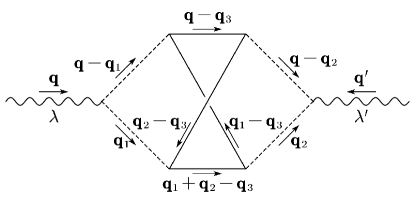
Figure 3: Feynman-like diagrams at $\mathcal{O}(f_{\mathrm{NL}}^{2})$ and $\mathcal{O}(f_{\mathrm{NL}}^{4})$ orders. They are specified as $H$ (Hybrid, top left), $C$ (top right), $Z$ (middle left), $R$ (Reducible, middle right), $P$ (Planar, bottom left), and $N$ (Non-Planar, bottom right) diagrams.

Therefore, we obtain seven Feynman-like diagrams that are related to nonvanishing contractions. They are depicted in the left panel of Fig. 2 and the panels of Fig. 3. Their contributions to the power spectrum in Eq. 4.1 can be obtained straightforwardly from the corresponding Feynman-like diagrams, as will be done in the following. Firstly, at $\mathcal{O}(f_{\mathrm{NL}}^{0})$ order, the contribution labeled by $G$ is corresponded to the left panel of Fig. 2, namely,

$$P_{h_{\lambda}}^{G}(\eta,q)=2^{5}\int\frac{\mathrm{d}^{3}\mathbf{q}_{1}}{(2\pi)^{3}}Q_{\lambda}^{2}(\mathbf{q},\mathbf{q}_{1})\hat{I}^{2}({\left|\mathbf{q}-\mathbf{q}_{1}\right|},q_{1},\eta)P_{g}(q_{1})P_{g}({\left|\mathbf{q}-\mathbf{q}_{1}\right|})\ .$$ (4.7)

It is exactly the result when $\zeta$ is Gaussian, as was studied in the literature [55, 56, 57, 58, 59, 60]. In contrast, all of the non-Gaussian contributions are plotted in Fig. 3. Secondly, at $\mathcal{O}(f_{\mathrm{NL}}^{2})$ order , they are labeled by $H$, $C$, and $Z$, and can be expressed as follows

$$P_{h_{\lambda}}^{H}(\eta,q) = 2^{7}\left(\frac{3}{5}f_{\mathrm{NL}}\right)^{2}\int\frac{\mathrm{d}^{3}\mathbf{q}_{1}}{(2\pi)^{3}}\frac{\mathrm{d}^{3}\mathbf{q}_{2}}{(2\pi)^{3}}P_{g}(q_{2})P_{g}({\left|\mathbf{q}-\mathbf{q}_{1}\right|})P_{g}({\left|\mathbf{q}_{1}-\mathbf{q}_{2}\right|})$$ (4.8)

$$\hphantom{\ 2^{8}\left(\frac{3}{5}f_{\mathrm{NL}}\right)^{2}}\times Q_{\lambda}^{2}(\mathbf{q},\mathbf{q}_{1})\hat{I}^{2}({\left|\mathbf{q}-\mathbf{q}_{1}\right|},q_{1},\eta)\ ,$$

$$P_{h_{\lambda}}^{C}(\eta,q) = 2^{8}\left(\frac{3}{5}f_{\mathrm{NL}}\right)^{2}\int\frac{\mathrm{d}^{3}\mathbf{q}_{1}}{(2\pi)^{3}}\frac{\mathrm{d}^{3}\mathbf{q}_{2}}{(2\pi)^{3}}P_{g}(q_{2})P_{g}({\left|\mathbf{q}-\mathbf{q}_{2}\right|})P_{g}({\left|\mathbf{q}_{1}-\mathbf{q}_{2}\right|})$$ (4.9)

$$\hphantom{\ 2^{8}\left(\frac{3}{5}f_{\mathrm{NL}}\right)^{2}}\times Q_{\lambda}(\mathbf{q},\mathbf{q}_{1})\hat{I}({\left|\mathbf{q}-\mathbf{q}_{1}\right|},q_{1},\eta)Q_{\lambda}(\mathbf{q},\mathbf{q}_{2})\hat{I}({\left|\mathbf{q}-\mathbf{q}_{2}\right|},q_{2},\eta)\ ,$$

$$P_{h_{\lambda}}^{Z}(\eta,q) = 2^{8}\left(\frac{3}{5}f_{\mathrm{NL}}\right)^{2}\int\frac{\mathrm{d}^{3}\mathbf{q}_{1}}{(2\pi)^{3}}\frac{\mathrm{d}^{3}\mathbf{q}_{2}}{(2\pi)^{3}}P_{g}(q_{2})P_{g}({\left|\mathbf{q}-\mathbf{q}_{1}\right|})P_{g}({\left|\mathbf{q}_{1}-\mathbf{q}_{2}\right|})$$ (4.10)

$$\hphantom{\ 2^{8}\left(\frac{3}{5}f_{\mathrm{NL}}\right)^{2}}\times Q_{\lambda}(\mathbf{q},\mathbf{q}_{1})\hat{I}({\left|\mathbf{q}-\mathbf{q}_{1}\right|},q_{1},\eta)Q_{\lambda}(\mathbf{q},\mathbf{q}_{2})\hat{I}({\left|\mathbf{q}-\mathbf{q}_{2}\right|},q_{2},\eta)\ .$$

Thirdly, at $\mathcal{O}(f_{\mathrm{NL}}^{4})$ order, they are labeled by $R$, $P$, and $N$, and can be expressed as follows

$$P_{h_{\lambda}}^{R}(\eta,q) = 2^{7}\left(\frac{3}{5}f_{\mathrm{NL}}\right)^{4}\int\frac{\mathrm{d}^{3}\mathbf{q}_{1}}{(2\pi)^{3}}\frac{\mathrm{d}^{3}\mathbf{q}_{2}}{(2\pi)^{3}}\frac{\mathrm{d}^{3}\mathbf{q}_{3}}{(2\pi)^{3}}P_{g}(q_{2})P_{g}(q_{3})P_{g}({\left|\mathbf{q}_{1}-\mathbf{q}_{2}\right|})$$

$$\hphantom{\ 2^{7}\left(\frac{3}{5}f_{\mathrm{NL}}\right)^{4}}\times P_{g}({\left|\mathbf{q}-\mathbf{q}_{1}-\mathbf{q}_{3}\right|})Q_{\lambda}^{2}(\mathbf{q},\mathbf{q}_{1})\hat{I}^{2}({\left|\mathbf{q}-\mathbf{q}_{1}\right|},q_{1},\eta)\ ,$$

$$P_{h_{\lambda}}^{P}(\eta,q) = 2^{9}\left(\frac{3}{5}f_{\mathrm{NL}}\right)^{4}\int\frac{\mathrm{d}^{3}\mathbf{q}_{1}}{(2\pi)^{3}}\frac{\mathrm{d}^{3}\mathbf{q}_{2}}{(2\pi)^{3}}\frac{\mathrm{d}^{3}\mathbf{q}_{3}}{(2\pi)^{3}}P_{g}(q_{3})P_{g}({\left|\mathbf{q}-\mathbf{q}_{3}\right|})P_{g}({\left|\mathbf{q}_{1}-\mathbf{q}_{3}\right|})$$

$$\hphantom{\ 2^{7}\left(\frac{3}{5}f_{\mathrm{NL}}\right)^{4}}\times P_{g}({\left|\mathbf{q}_{2}-\mathbf{q}_{3}\right|})Q_{\lambda}(\mathbf{q},\mathbf{q}_{1})\hat{I}({\left|\mathbf{q}-\mathbf{q}_{1}\right|},q_{1},\eta)$$

$$\hphantom{\ 2^{7}\left(\frac{3}{5}f_{\mathrm{NL}}\right)^{4}}\times Q_{\lambda}(\mathbf{q},\mathbf{q}_{2})\hat{I}({\left|\mathbf{q}-\mathbf{q}_{2}\right|},q_{2},\eta)\ ,$$

$$P_{h_{\lambda}}^{N}(\eta,q) = 2^{8}\left(\frac{3}{5}f_{\mathrm{NL}}\right)^{4}\int\frac{\mathrm{d}^{3}\mathbf{q}_{1}}{(2\pi)^{3}}\frac{\mathrm{d}^{3}\mathbf{q}_{2}}{(2\pi)^{3}}\frac{\mathrm{d}^{3}\mathbf{q}_{3}}{(2\pi)^{3}}P_{g}({\left|\mathbf{q}-\mathbf{q}_{3}\right|})P_{g}({\left|\mathbf{q}_{1}-\mathbf{q}_{3}\right|})$$

$$\hphantom{\ 2^{7}\left(\frac{3}{5}f_{\mathrm{NL}}\right)^{4}}\times P_{g}({\left|\mathbf{q}_{1}+\mathbf{q}_{2}-\mathbf{q}_{3}\right|})P_{g}({\left|\mathbf{q}_{2}-\mathbf{q}_{3}\right|})Q_{\lambda}(\mathbf{q},\mathbf{q}_{1})$$

$$\hphantom{\ 2^{7}\left(\frac{3}{5}f_{\mathrm{NL}}\right)^{4}}\times\hat{I}({\left|\mathbf{q}-\mathbf{q}_{1}\right|},q_{1},\eta)Q_{\lambda}(\mathbf{q},\mathbf{q}_{2})\hat{I}({\left|\mathbf{q}-\mathbf{q}_{2}\right|},q_{2},\eta)\ .$$

Here, we have taken into account the symmetry factor for each Feynman-like diagram. Following Eq. 4.3, for each Feynman-like diagram, we can determine its contribution to $\bar{\Omega}_{\mathrm{gw}}(\eta,q)$, which is labeled by the same superscript as the one labelling the Feynman-like diagram.

The study of GW induced by the primordial scalar perturbations with local-type non-Gaussianity was first conducted in Ref. [49]. The authors considered only the contributions labeled by $G$, $H$, and $R$. Subsequently, other contributions, except the one labeled by $Z$, were investigated in Ref. [50]. The contribution labeled by $Z$ was first computed in Ref. [52]. It is worth noting that the contribution labeled by $C$ is referred to as “walnut” in Ref. [50], while “walnut” is used to denote the one labeled by $Z$ in Ref. [52]. The first complete analysis and the Feynman-like rules and diagrams have been provided by Ref. [53], which is followed by our current work. Corresponding to the above papers, we compare their results in Fig. 4, which will be numerically reproduced in the next subsection. In addition, the scale-dependent non-Gaussianity was studied in Ref. [54].

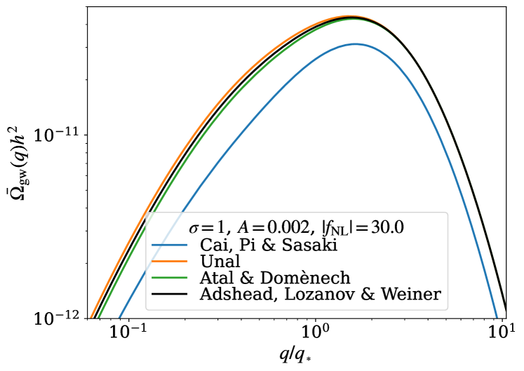
Figure 4: Comparison of the energy-density fraction spectra of SIGW provided by Ref. [49] (blue curve), Ref. [50] (orange curve), Ref. [52] (green curve), and Ref. [53] (black curve). Here, we reproduce the complete results analyzed by Ref. [53].

Based on Eq. 4.3, we straightforwardly obtain contributions from the above seven integrals to the energy-density fraction spectrum. Therefore, the total spectrum is determined by a sum of them, i.e.,

$$\bar{\Omega}_{\mathrm{gw}}(\eta,q)=\bar{\Omega}_{\mathrm{gw}}^{G}+\bar{\Omega}_{\mathrm{gw}}^{H}+\bar{\Omega}_{\mathrm{gw}}^{C}+\bar{\Omega}_{\mathrm{gw}}^{Z}+\bar{\Omega}_{\mathrm{gw}}^{R}+\bar{\Omega}_{\mathrm{gw}}^{P}+\bar{\Omega}_{\mathrm{gw}}^{N}\ .$$ (4.14)

Based on the above derivations, it is obvious that each contribution to the total spectrum $\bar{\Omega}_{\mathrm{gw}}(\eta,q)$ does not explicitly contain $\eta$ in the limit of $x\gg 1$. Therefore, $n_{\mathrm{gw}}(\eta,q)$ defined in Eq. 2.23 is independent of $\eta$. In light of the tensor transfer function, the spectrum at current time $\eta_{0}$ had been presented, e.g., in Ref. [92]. It is given as

$$\bar{\Omega}_{\mathrm{gw}}(q) = \Omega_{\mathrm{rad},0}\left(\frac{g_{*,\rho,\mathrm{e}}}{g_{*,\rho,0}}\right)\left(\frac{g_{*,s,0}}{g_{*,s,\mathrm{e}}}\right)^{4/3}\bar{\Omega}_{\mathrm{gw}}(\eta,q)\ ,$$ (4.15)

where the subscripts ₀ and _e label the present time and the emission time, respectively. The energy-density fraction of radiations today is $\Omega_{\mathrm{rad},0}=4.2\times 10^{-5}h^{-2}$, where $h=0.6736$ is the dimensionless Hubble constant [115]. The effective numbers of relativistic species, i.e., $g_{\ast,\rho}$ and $g_{\ast,s}$, can be obtained from the tabulated data shown in Ref. [116].

4.3 Numerical results

In order to calculate the above seven integrals numerically, it is convenient to classify them into two categories. The first category contains the integrals labeled by $G$, $H$, and $R$, while the second one contains those labeled by $C$, $Z$, $P$, and $N$.

For the first category, we introduce three sets of new variables $(u_{i},v_{i})$, namely,

$$v_{1} = \frac{q_{1}}{q}\ ,\qquad\qquad\qquad u_{1}=\frac{{\left|\mathbf{q}-\mathbf{q}_{1}\right|}}{q}\ ,$$ (4.16a)

$$v_{2} = \frac{q_{2}}{q_{1}}\ ,\qquad\qquad\qquad u_{2}=\frac{{\left|\mathbf{q}_{1}-\mathbf{q}_{2}\right|}}{q_{1}}\ ,$$ (4.16b)

$$v_{3} = \frac{q_{3}}{{\left|\mathbf{q}-\mathbf{q}_{1}\right|}}\ ,\qquad\quad\ \,u_{3}=\frac{{\left|\mathbf{q}-\mathbf{q}_{1}-\mathbf{q}_{3}\right|}}{{\left|\mathbf{q}-\mathbf{q}_{1}\right|}}\ ,$$ (4.16c)

During RD epoch, we have $\hat{I}({\left|\mathbf{q}-\mathbf{q}_{1}\right|},q_{1},\eta)=I_{\mathrm{RD}}(u_{1},v_{1},x)$ with $x=q\eta$, as was shown in Eq. 3.15. For simplification, we introduce a new quantity

$$J(u_{1},v_{1},x)=\frac{x}{8}\bigl{[}(v_{1}+u_{1})^{2}-1\bigr{]}\bigl{[}1-(v_{1}-u_{1})^{2}\bigr{]}I_{\mathrm{RD}}(u_{1},v_{1},x)\ ,$$ (4.17)

where the explicit expression of $I_{\mathrm{RD}}(u_{1},v_{1},x)$ when $x\rightarrow\infty$ was shown in Eq. 3.16. After explicit computation, we get

$$J^{2}(u_{1},v_{1},x)=x^{2}\sum_{\lambda}Q_{\lambda}^{2}(\mathbf{q},\mathbf{q}_{1})\hat{I}^{2}({\left|\mathbf{q}-\mathbf{q}_{1}\right|},q_{1},\eta)\ .$$ (4.18)

Due to the oscillation average, we have

$$\mkern 1.5mu\overline{\mkern-1.5muJ^{2}(u_{1},v_{1},x\rightarrow\infty)\mkern-1.5mu}\mkern 1.5mu=\frac{x^{2}}{64}\bigl{[}(v_{1}+u_{1})^{2}-1\bigr{]}^{2}\bigl{[}1-(v_{1}-u_{1})^{2}\bigr{]}^{2}\mkern 1.5mu\overline{\mkern-1.5muI_{\mathrm{RD}}^{2}(u_{1},v_{1},x\rightarrow\infty)\mkern-1.5mu}\mkern 1.5mu\ ,$$ (4.19)

which can be obtained from Eq. (3.17). In fact, Eq. 4.19 is independent of $x$. To transform the integration region into a rectangle, we define the transformation of variables as follows

$$s_{i}=u_{i}-v_{i}\ ,\qquad\qquad\quad t_{i}=u_{i}+v_{i}-1\ .$$ (4.20)

After considering the Jacobian, we obtain the contributions to $\bar{\Omega}_{\mathrm{gw}}(\eta,q)$ from the integrals labeled as $G$, $H$ and $R$, respectively. They are given as

$$\bar{\Omega}_{\mathrm{gw}}^{G}(\eta,q) = \frac{1}{3}\int_{0}^{\infty}\mathrm{d}t_{1}\int_{-1}^{1}\mathrm{d}s_{1}\mkern 1.5mu\overline{\mkern-1.5muJ^{2}(u_{1},v_{1},x\rightarrow\infty)\mkern-1.5mu}\mkern 1.5mu\frac{1}{(u_{1}v_{1})^{2}}\Delta^{2}_{g}(v_{1}q)\Delta^{2}_{g}(u_{1}q)\ ,$$ (4.21)

$$\bar{\Omega}_{\mathrm{gw}}^{H}(\eta,q) = \frac{1}{3}\left(\frac{3f_{\mathrm{NL}}}{5}\right)^{2}\prod_{i=1}^{2}\biggl{[}\int_{0}^{\infty}\mathrm{d}t_{i}\int_{-1}^{1}\mathrm{d}s_{i}\biggr{]}\mkern 1.5mu\overline{\mkern-1.5muJ^{2}(u_{1},v_{1},x\rightarrow\infty)\mkern-1.5mu}\mkern 1.5mu\frac{1}{(u_{1}v_{1}u_{2}v_{2})^{2}}$$ (4.22)

$$\hphantom{\left(\frac{3f_{\mathrm{NL}}}{5}\right)^{2}\frac{1}{12}\biggl{[}\int_{0}^{\infty}\biggr{]}}\times\Delta^{2}_{g}(v_{1}v_{2}q)\Delta^{2}_{g}(u_{1}q)\Delta^{2}_{g}(v_{1}u_{2}q)\ ,$$

$$\bar{\Omega}_{\mathrm{gw}}^{R}(\eta,q) = \frac{1}{12}\left(\frac{3f_{\mathrm{NL}}}{5}\right)^{4}\prod_{i=1}^{3}\biggl{[}\int_{0}^{\infty}\mathrm{d}t_{i}\int_{-1}^{1}\mathrm{d}s_{i}\biggr{]}\mkern 1.5mu\overline{\mkern-1.5muJ^{2}(u_{1},v_{1},x\rightarrow\infty)\mkern-1.5mu}\mkern 1.5mu\frac{1}{(u_{1}v_{1}u_{2}v_{2}u_{3}v_{3})^{2}}$$ (4.23)

$$\hphantom{\left(\frac{3f_{\mathrm{NL}}}{5}\right)^{2}\frac{1}{12}\biggl{[}\int_{0}^{\infty}\biggr{]}}\times\Delta^{2}_{g}(v_{1}v_{2}q)\Delta^{2}_{g}(v_{1}u_{2}q)\Delta^{2}_{g}(u_{1}v_{3}q)\Delta^{2}_{g}(u_{1}u_{3}q)\ .$$

The above three integrals can be numerically computed by the vegas [117] package.

For the second category, we also introduce three sets of new variables, still labeled by $(u_{i},v_{i})$ with $i=1,2,3$, namely,

$$v_{i}=\frac{q_{i}}{q}\ ,\qquad\qquad\quad u_{i}=\frac{{\left|\mathbf{q}-\mathbf{q}_{i}\right|}}{q}\ ,$$ (4.24)

which are different from those in Eq. (4.16). Since the definition of $(v_{1},u_{1})$ in Eq. 4.24 is the same as that in Eq. 4.16a, the definition of $J(u_{1},v_{1},x)$ in Eq. 4.17 is still applicable for $(u_{1},v_{1})$ in Eq. 4.24. Here, we further redefine it in a more general way, i.e.,

$$J(u_{i},v_{i},x)=\frac{x}{8}\bigl{[}(v_{i}+u_{i})^{2}-1\bigr{]}\bigl{[}1-(v_{i}-u_{i})^{2}\bigr{]}I_{\mathrm{RD}}(u_{i},v_{i},x)\ ,$$ (4.25)

where the explicit expression of $I_{\mathrm{RD}}(u_{i},v_{i},x)$ when $x\rightarrow\infty$ was still shown in Eq. 3.16. After explicit computation, we get

$$J(u_{1},v_{1},x)J(u_{2},v_{2},x)\cos 2\varphi_{12}=x^{2}\sum_{\lambda}Q_{\lambda}(\mathbf{q},\mathbf{q}_{1})\hat{I}({\left|\mathbf{q}-\mathbf{q}_{1}\right|},q_{1},\eta)Q_{\lambda}(\mathbf{q},\mathbf{q}_{2})\hat{I}({\left|\mathbf{q}-\mathbf{q}_{2}\right|},q_{2},\eta)\ ,$$ (4.26)

where we denote $\varphi_{ij}=\phi_{i}-\phi_{j}$ for the sake of brevity, and the azimuthal angle $\phi_{i}$ has been defined in Section 3.1. The oscillation average of $J(u_{1},v_{1},x)J(u_{2},v_{2},x)$ can be obtained via Eq. (3.17), i.e.,

$$\mkern 1.5mu\overline{\mkern-1.5muJ(u_{1},v_{1},x\rightarrow\infty)J(u_{2},v_{2},x\rightarrow\infty)\mkern-1.5mu}\mkern 1.5mu = \frac{x^{2}}{64}\bigl{[}(v_{1}+u_{1})^{2}-1\bigr{]}\bigl{[}1-(v_{1}-u_{1})^{2}\bigr{]}$$

$$\times\bigl{[}(v_{2}+u_{2})^{2}-1\bigr{]}\bigl{[}1-(v_{2}-u_{2})^{2}\bigr{]}$$

$$\times\mkern 1.5mu\overline{\mkern-1.5muI_{\mathrm{RD}}(u_{1},v_{1},x\rightarrow\infty)I_{\mathrm{RD}}(u_{2},v_{2},x\rightarrow\infty)\mkern-1.5mu}\mkern 1.5mu\ ,$$

which is also independent of $x$. The transformation from $(u_{i},v_{i})$ to $(s_{i},t_{i})$ remains the same as that in Eq. (4.20). For simplification, we introduce a new quantity

$$y_{ij}=\frac{\mathbf{q}_{i}\cdot\mathbf{q}_{j}}{q^{2}} = \frac{\cos\varphi_{ij}}{4}\sqrt{t_{i}(t_{i}+2)(1-s_{i}^{2})t_{j}(t_{j}+2)(1-s_{j}^{2})}$$ (4.28)

$$+\frac{1}{4}[1-s_{i}(t_{i}+1)][1-s_{j}(t_{j}+1)]\ ,$$

and further define two new quantities as follows

$$w_{ij} = \frac{{\left|\mathbf{q}_{i}-\mathbf{q}_{j}\right|}}{q}=\sqrt{v_{i}^{2}+v_{j}^{2}-y_{ij}}\ ,$$ (4.29)

$$w_{123} = \frac{{\left|\mathbf{q}_{1}+\mathbf{q}_{2}-\mathbf{q}_{3}\right|}}{q}=\sqrt{v_{1}^{2}+v_{2}^{2}+v_{3}^{2}+y_{12}-y_{13}-y_{23}}\ .$$ (4.30)

After considering the Jacobian, we obtain the contributions to $\bar{\Omega}_{\mathrm{gw}}(\eta,q)$ from the integrals labeled as $C$, $Z$, $P$, and $N$, respectively. They are given as

$$\bar{\Omega}_{\mathrm{gw}}^{C}(\eta,q) = \frac{1}{3\pi}\left(\frac{3f_{\mathrm{NL}}}{5}\right)^{2}\prod_{i=1}^{2}\biggl{[}\int_{0}^{\infty}\mathrm{d}t_{i}\int_{-1}^{1}\mathrm{d}s_{i}\,v_{i}u_{i}\biggr{]}\int_{0}^{2\pi}\mathrm{d}\varphi_{12}\,\cos 2\varphi_{12}$$

$$\hphantom{\left(\frac{3f_{\mathrm{NL}}}{5}\right)^{2}\frac{1}{12\pi}\prod_{i=1}^{2}}\times\mkern 1.5mu\overline{\mkern-1.5muJ(u_{1},v_{1},x\rightarrow\infty)J(u_{2},v_{2},x\rightarrow\infty)\mkern-1.5mu}\mkern 1.5mu$$

$$\hphantom{\left(\frac{3f_{\mathrm{NL}}}{5}\right)^{2}\frac{1}{12\pi}\prod_{i=1}^{2}}\times\frac{\Delta^{2}_{g}(v_{2}q)}{v_{2}^{3}}\frac{\Delta^{2}_{g}(u_{2}q)}{u_{2}^{3}}\frac{\Delta^{2}_{g}(w_{12}q)}{w_{12}^{3}}\ ,$$

$$\bar{\Omega}_{\mathrm{gw}}^{Z}(\eta,q) = \frac{1}{3\pi}\left(\frac{3f_{\mathrm{NL}}}{5}\right)^{2}\prod_{i=1}^{2}\biggl{[}\int_{0}^{\infty}\mathrm{d}t_{i}\int_{-1}^{1}\mathrm{d}s_{i}\,v_{i}u_{i}\biggr{]}\int_{0}^{2\pi}\mathrm{d}\varphi_{12}\,\cos 2\varphi_{12}$$

$$\hphantom{\left(\frac{3f_{\mathrm{NL}}}{5}\right)^{2}\frac{1}{12\pi}\prod_{i=1}^{2}}\times\mkern 1.5mu\overline{\mkern-1.5muJ(u_{1},v_{1},x\rightarrow\infty)J(u_{2},v_{2},x\rightarrow\infty)\mkern-1.5mu}\mkern 1.5mu$$

$$\hphantom{\left(\frac{3f_{\mathrm{NL}}}{5}\right)^{2}\frac{1}{12\pi}\prod_{i=1}^{2}}\times\frac{\Delta^{2}_{g}(v_{2}q)}{v_{2}^{3}}\frac{\Delta^{2}_{g}(u_{1}q)}{u_{1}^{3}}\frac{\Delta^{2}_{g}(w_{12}q)}{w_{12}^{3}}\ ,$$

$$\bar{\Omega}_{\mathrm{gw}}^{P}(\eta,q) = \frac{1}{24\pi^{2}}\left(\frac{3f_{\mathrm{NL}}}{5}\right)^{4}\prod_{i=1}^{3}\biggl{[}\int_{0}^{\infty}\mathrm{d}t_{i}\int_{-1}^{1}\mathrm{d}s_{i}\,v_{i}u_{i}\biggr{]}\int_{0}^{2\pi}\mathrm{d}\varphi_{12}\mathrm{d}\varphi_{23}\,\cos 2\varphi_{12}$$

$$\hphantom{\left(\frac{3f_{\mathrm{NL}}}{5}\right)^{4}\frac{1}{96\pi^{2}}\prod_{i=1}^{3}}\times\mkern 1.5mu\overline{\mkern-1.5muJ(u_{1},v_{1},x\rightarrow\infty)J(u_{2},v_{2},x\rightarrow\infty)\mkern-1.5mu}\mkern 1.5mu$$

$$\hphantom{\left(\frac{3f_{\mathrm{NL}}}{5}\right)^{4}\frac{1}{96\pi^{2}}\prod_{i=1}^{3}}\times\frac{\Delta^{2}_{g}(v_{3}q)}{v_{3}^{3}}\frac{\Delta^{2}_{g}(u_{3}q)}{u_{3}^{3}}\frac{\Delta^{2}_{g}(w_{13}q)}{w_{13}^{3}}\frac{\Delta^{2}_{g}(w_{23}q)}{w_{23}^{3}}\ ,$$

$$\bar{\Omega}_{\mathrm{gw}}^{N}(\eta,q) = \frac{1}{24\pi^{2}}\left(\frac{3f_{\mathrm{NL}}}{5}\right)^{4}\prod_{i=1}^{3}\biggl{[}\int_{0}^{\infty}\mathrm{d}t_{i}\int_{-1}^{1}\mathrm{d}s_{i}\,v_{i}u_{i}\biggr{]}\int_{0}^{2\pi}\mathrm{d}\varphi_{12}\mathrm{d}\varphi_{23}\,\cos 2\varphi_{12}$$

$$\hphantom{\left(\frac{3f_{\mathrm{NL}}}{5}\right)^{4}\frac{1}{96\pi^{2}}\prod_{i=1}^{3}}\times\mkern 1.5mu\overline{\mkern-1.5muJ(u_{1},v_{1},x\rightarrow\infty)J(u_{2},v_{2},x\rightarrow\infty)\mkern-1.5mu}\mkern 1.5mu$$

$$\hphantom{\left(\frac{3f_{\mathrm{NL}}}{5}\right)^{4}\frac{1}{96\pi^{2}}\prod_{i=1}^{3}}\times\frac{\Delta^{2}_{g}(u_{3}q)}{u_{3}^{3}}\frac{\Delta^{2}_{g}(w_{13}q)}{w_{13}^{3}}\frac{\Delta^{2}_{g}(w_{23}q)}{w_{23}^{3}}\frac{\Delta^{2}_{g}(w_{123}q)}{w_{123}^{3}}\ .$$

The above four integrals can also be numerically computed by the vegas [117] package.

We postulate that the dimensionless power spectrum of the Gaussian primordial curvature perturbations $\zeta_{g}$ is given by a normal function with respect to $\ln q$, i.e.,

$$\Delta^{2}_{g}(q)=\frac{A}{\sqrt{2\pi\sigma^{2}}}\exp\left(-\frac{\ln^{2}(q/q_{\ast})}{2\sigma^{2}}\right)\ ,$$ (4.35)

where $q_{\ast}$ denotes the spectral peak, $\sigma$ stands for the standard deviation, and $A$ is the the spectral amplitude at $q_{\ast}$. This power spectrum has been broadly used in the literature, e.g., Refs. [118, 53, 73, 119].

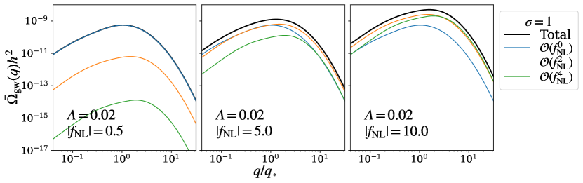
Figure 5: Energy-density fraction spectrum of SIGW in the current universe. We let $A=0.02$, $\sigma=1$, and $f_{\mathrm{NL}}=0.5,~{}5.0,~{}10.0$ from left to right panels. The Gaussian contribution, which is of $\mathcal{O}(f_{\mathrm{NL}}^{0})$ order, is denoted by a blue line in each panel, while the non-Gaussian contributions of $\mathcal{O}(f_{\mathrm{NL}}^{2})$ and $\mathcal{O}(f_{\mathrm{NL}}^{4})$ orders are denoted by orange and green curves, respectively. The total spectra are shown as black curves.

In Fig. 5, we show the contributions of primordial non-Gaussianity, which depend on powers of $f_{\mathrm{NL}}^{2}$ (exactly speaking, powers of $Af_{\mathrm{NL}}^{2}$), to the energy-density fraction spectrum $\bar{\Omega}_{\mathrm{gw},0}(q)$ in Eq. (4.15). Here, we let $A=0.02$, $\sigma=1$, but vary $|f_{\mathrm{NL}}|$ via letting it to be $0.5$, $5.0$, and $10.0$ from the left to right panels. Throughout this paper, we manipulate $f_{\mathrm{NL}}$ to insure that the non-Gaussian contribution to $\zeta$ in Eq. 4.4 lies in perturbative regime, i.e., $(3f_{\mathrm{NL}}/5)^{2}A<1$. However, we would not require the constraints on $f_{\mathrm{NL}}$ from CMB, since we are discussing couplings between long-wavelength modes, that could be related to CMB, and extremely-short-wavelength modes that are beyond the scope of CMB observations. Therefore, the CMB bounds are irrelevant to our current work. In addition, we depict the Gaussian contribution that is of $\mathcal{O}(f_{\mathrm{NL}}^{0})$ order, following Refs. [59, 60, 53]. It is denoted by blue curves in the panels. As were shown in Refs. [46, 47, 49, 50, 51, 52, 53], the non-Gaussian contributions become more significant with increase of $|f_{\mathrm{NL}}|$, and could be dominant for $|f_{\mathrm{NL}}|\sim\mathcal{O}(10)$. Compared with the Gaussian contribution, they are negligible for $|f_{\mathrm{NL}}|\sim\mathcal{O}(0.1)$, comparable for $|f_{\mathrm{NL}}|\sim\mathcal{O}(1)$, and one order of magnitude larger for $|f_{\mathrm{NL}}|\sim\mathcal{O}(10)$. Further, the contribution of $\mathcal{O}(f_{\mathrm{NL}}^{4})$ order also becomes more significant with increase of $|f_{\mathrm{NL}}|$, and could be comparable to that of $\mathcal{O}(f_{\mathrm{NL}}^{2})$ order for $|f_{\mathrm{NL}}|\sim\mathcal{O}(10)$. In fact, the above results are available for $A\sim\mathcal{O}(10^{-3}-10^{-1})$, i.e., the value of spectral amplitude commonly used in scenarios of PBH production.

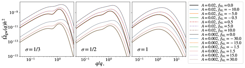
Figure 6: Dependence of the energy-density fraction spectrum of SIGW in the current universe on the parameters $A$ and $\sigma$, as well as the sign degeneracy of $f_{\mathrm{NL}}$. For $A=0.02$ ($A=0.002$), positive values of $f_{\mathrm{NL}}$ are denoted by solid (dashed) curves, while negative ones are denoted by dot-dashed (dotted) curves. For the Gaussian perturbations, i.e., $f_{\mathrm{NL}}=0$, we denote the results of $A=0.02$ and $A=0.002$ with black and gray curves, respectively.

In Fig. 6, we also show the dependence of $\bar{\Omega}_{\mathrm{gw}}(q)$ on the parameters $A$ and $\sigma$, as well as the sign degeneracy of $f_{\mathrm{NL}}$. The spectral magnitude strongly depends on $A$ (as well as $f_{\mathrm{NL}}$), as is shown in Refs. [55, 53]. Larger value of $A$ leads to a larger spectral magnitude, roughly following $\bar{\Omega}_{\mathrm{gw}}\propto A^{2}$, and vice versa. In contrast, the variation of $\sigma$ mainly alters the shape of spectral profile, as is demonstrated in Fig. 6 from the left to right panels. Furthermore, there is a sign degeneracy of $f_{\mathrm{NL}}$, because $\bar{\Omega}_{\mathrm{gw}}(q)$ depends on powers of $f_{\mathrm{NL}}^{2}$ in Eq. (4.21)–Eq. (4.23) and Eq. (4.3)–Eq. (4.3). Therefore, we can obtain at most the value of $|f_{\mathrm{NL}}|$, rather than $f_{\mathrm{NL}}$, via measuring the monopole in SIGW.

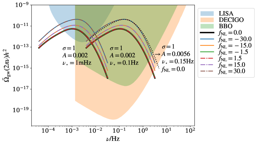
Figure 7: Energy-density fraction spectra of SIGW in the current universe against the sensitivity curves of LISA (blue shaded region) [120, 121], DECIGO (orange shaded region) [122, 123], and BBO (green shaded region) [124, 125]. Positive and vanishing values of $f_{\mathrm{NL}}$ are denoted by solid curves, while negative ones are denoted by dot-dashed curves. In addition, the dotted curve denotes the spectrum with $A=0.0056$, $\sigma=1$, $f_{\mathrm{NL}}=0.0$, and $\nu_{\ast}=0.15$ Hz.

As shown in Fig. 7, the anticipated spectrum $\bar{\Omega}_{\mathrm{gw}}$ is potentially measurable for future space-borne GW detectors, e.g., LISA [120, 121], DECIGO [122, 123], and BBO [124, 125]. Here, the GW frequency is $\nu=q/(2\pi)$ and the pivot frequency is $\nu_{\ast}=q_{\ast}/(2\pi)$. Letting $A=0.002$ and $\sigma=1$, but varying the value of $f_{\mathrm{NL}}$, we depict the spectra $\bar{\Omega}_{\mathrm{gw}}(2\pi\nu)$ for $\nu_{\ast}=1$ mHz and $\nu_{\ast}=0.1$ Hz, which are corresponded to the LISA band and the DECIGO/BBO band, respectively. Based on Fig. 7, we expect these detectors to probe SIGW related to the parameter region (particularly, the intervals of $A$ and $f_{\mathrm{NL}}$) that exerts a significant impact on the formation of PBH, in particular, the abundance [81, 82, 83].

Besides the sign degeneracy of $f_{\mathrm{NL}}$, there are other degeneracies in the model parameters including $A$, $\sigma$, $f_{\mathrm{NL}}$, and $\nu_{\ast}$. As an example, we depict the spectrum $\bar{\Omega}_{\mathrm{gw}}(\nu)$ for $A=0.0056$, $\sigma=1$, $f_{\mathrm{NL}}=0.0$, and $\nu_{\ast}=0.15$ Hz, as is denoted by the dotted curve in Fig. 7. We find that it almost coincides with the spectra with $A=0.002$, $\sigma=1$, $f_{\mathrm{NL}}=\pm 30.0$, and $\nu_{\ast}=0.1$ Hz, indicating that it is very challenging to determine the value of $|f_{\mathrm{NL}}|$ with measurements of the monopole in SIGW only. In fact, only a combination of the form $Af_{\mathrm{NL}}^{2}$, rather than $f_{\mathrm{NL}}$ itself, contributes to the energy-density fraction spectrum.

In summary, it is imperative to develop new probes of the primordial non-Gaussianity through potential measurements of SIGW.

5 Multipoles and primordial non-Gaussianity

In this section, we study the anisotropies in SIGW contributed by the local-type primordial non-Gaussianity in curvature perturbations, and then show the first complete analysis to the angular power spectrum of SIGW. The method and analytic formulae developed in this section could be generalized straightforwardly, e.g., to study the anisotropies in SIGW produced during matter domination.

5.1 Angular power spectrum

The correlation of initial perturbations, i.e., $\delta(\eta_{\mathrm{in}},\mathbf{x}_{\mathrm{in}},\mathbf{q})$ in Eq. (2.2), at two different locations separated by a large angle (i.e., low multipoles) can only arise from the PNG. The local-type PNG leads to the coupling between modes of short-wavelength and long-wavelength [126]. In this subsection, we will adopt the Feynman-like diagrams to compute two-point correlations of the initial inhomogeneities.

In Fourier space, we can decompose the Gaussian component of curvature perturbation $\zeta$ in Eq. 4.4 as follows

$$\zeta_{g}(\mathbf{k})=\zeta_{S}(\mathbf{k})+\zeta_{L}(\mathbf{k})\ ,$$ (5.1)

where the suffixes _S and _L denote the short-wavelength and long-wavelength modes, respectively. We define the power spectra of these modes as

$$\langle\zeta_{S}(\mathbf{q})\zeta_{S}(\mathbf{q}^{\prime})\rangle = \delta^{(3)}(\mathbf{q}+\mathbf{q}^{\prime})P_{S}(q)\ ,$$ (5.2a)

$$\langle\zeta_{L}(\mathbf{k})\zeta_{L}(\mathbf{k}^{\prime})\rangle = \delta^{(3)}(\mathbf{k}+\mathbf{k}^{\prime})P_{L}(k)\ ,$$ (5.2b)

$$\langle\zeta_{S}(\mathbf{q})\zeta_{L}(\mathbf{k})\rangle = 0\ .$$ (5.2c)

For the long-wavelength modes, the dimensionless power spectrum $\Delta^{2}_{L}$ is nearly scale-invariant, with the spectral amplitude $A_{L}\simeq 2.1\times 10^{-9}$ [115]. In contrast, for the short-wavelength modes, the spectral amplitude $A_{S}$ is nearly unconstrained by current observations. In this work, assuming the dimensionless power spectrum in Eq. 4.35, we consider the spectral amplitude $A_{S}=A\sim\mathcal{O}(10^{-3}-10^{-1})$, which is related to the formation scenarios of PBH (e.g., see Refs. [127, 107]).

To simplify computation of the angular power spectrum in Eq. 2.15, we make several approximations to the density contrast in SIGW in Eq. (2.2). Firstly, besides $\Phi(\eta_{0},\mathbf{x}_{0})$, we disregard the tensor sourced term which is contributed by the primordial GW and SIGW smaller than the linear scalar perturbations. Secondly, the ISW effect is subdominant and thus can be neglected, as was shown in Ref. [100]. Thirdly, we have demonstrated in Section 4.2 that $n_{\mathrm{gw}}(\eta,q)$ is independent of $\eta$. Therefore, we approximate Eq. (2.2) as

$$\delta_{\mathrm{gw}}(\mathbf{q})=\delta_{\mathrm{gw}}(\eta_{\mathrm{in}},\mathbf{x}_{\mathrm{in}},\mathbf{q})+\left[4-n_{\mathrm{gw}}(q)\right]\Phi(\eta_{\mathrm{in}},\mathbf{x}_{\mathrm{in}})\ ,$$ (5.3)

where we denote $n_{\mathrm{gw}}(q)=n_{\mathrm{gw}}(\eta_{0},q)$ for simplicity. On the right hand side of Eq. (5.3), the first term denotes the initial inhomogeneities, while the second one leads to the SW effect. Since the angular resolution is finite for a GW detector, the signal along a line-of-sight is actually an ensemble average of the energy density of SIGW over a large quantity of Hubble horizons. In this sense, the initial inhomogeneities in a neighborhood of $\mathbf{x}_{\mathrm{in}}$ can be viewed to be isotropic. However, the initial inhomogeneities around $\mathbf{x}_{\mathrm{in}}$ and $\mathbf{x}_{\mathrm{in}}^{\prime}$ separated by a long distance could be correlated due to the PNG, as will be computed with the Feynman-like diagrams in the following.

In addition, the SW effect is produced by the long-wavelength scalar modes that reentered into the Hubble horizon during matter domination, indicating $w=c_{s}^{2}=0$. Based on Eq. (3.9) and Eq. (3.5), we get the scalar transfer function to be $T(k\eta)=1$ during matter domination. Therefore, we have

$$\Phi(\eta_{\mathrm{in}},\mathbf{x}_{\mathrm{in}})=\frac{3}{5}\int\frac{\mathrm{d}^{3}\mathbf{k}}{(2\pi)^{3/2}}e^{i\mathbf{k}\cdot\mathbf{x}_{\mathrm{in}}}\zeta_{L}(\mathbf{k})\ ,$$ (5.4)

which should be substituted back into Eq. (5.3). Here, we consider the linear term in $\zeta_{L}$ only, since higher-order terms are much smaller than this term due to $A_{L}\sim 10^{-9}$.

5.1.1 Feynman-like rules

To get the initial inhomogeneities $\delta_{\mathrm{gw}}(\eta_{\mathrm{in}},\mathbf{x}_{\mathrm{in}},\mathbf{q})$, it is necessary to compute the initial energy-density full spectrum $\omega_{\mathrm{gw}}(\eta_{\mathrm{in}},\mathbf{x}_{\mathrm{in}},\mathbf{q})$ first of all, based on Eq. 2.11 and Eq. 2.12. Following Eq. 2.8, we obtain the latter to be

$$\omega_{\mathrm{gw}}(\eta_{\mathrm{in}},\mathbf{x}_{\mathrm{in}},\mathbf{q})=-\frac{q^{3}}{48\mathcal{H}^{2}}\int\frac{\mathrm{d}^{3}\mathbf{k}}{(2\pi)^{3}}e^{i\mathbf{k}\cdot\mathbf{x}_{\mathrm{in}}}\left(\mathbf{k}-\mathbf{q}\right)\cdot\mathbf{q}\sum_{\lambda,\lambda^{\prime}}\epsilon_{ij}^{\lambda}(\mathbf{k}-\mathbf{q})\epsilon_{ij}^{\lambda^{\prime}}(\mathbf{q})\mkern 1.5mu\overline{\mkern-1.5muh_{\lambda}(\eta,\mathbf{k}-\mathbf{q})h_{\lambda^{\prime}}(\eta,\mathbf{q})\mkern-1.5mu}\mkern 1.5mu\ .$$ (5.5)

Here, $\mathbf{q}$ denotes a comoving momentum of GW that is corresponded to the short-wavelength, while $\mathbf{k}$ is associated with a Fourier mode of the inhomogeneities in SIGW, that is corresponded to the long-wavelength. We will take $q\gtrsim\mathcal{H}^{-1}\gg k$ in the following.

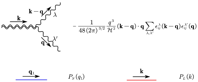
Figure 8: Feynman-like rules supplemented for the evaluation of SIGW. The double wavy line denotes the energy-density full spectrum $\omega_{\mathrm{gw}}(\eta,\mathbf{k},\mathbf{q})$, the blue solid line represents $P_{S}$, and the red solid line stands for $P_{L}$. Note that the Feynman-like rule in the top panel includes an operator.

The statistics of the inhomogeneities in SIGW is expressed as a two-point correlator $\langle\omega_{\mathrm{gw}}(\eta_{\mathrm{in}},\mathbf{x}_{\mathrm{in}},\mathbf{q})\omega_{\mathrm{gw}}(\eta_{\mathrm{in}},\mathbf{x}_{\mathrm{in}}^{\prime},\mathbf{q}^{\prime})\rangle$. By substituting Eq. 3.10 into Eq. 5.5, we can rewrite the latter in terms of an eight-point correlator of $\zeta$. Utilizing Eq. 4.4, Eq. 5.1, and Eq. 5.2a, we further rewrite it in terms of two-point correlators of the Gaussian components $\zeta_{S}$ and $\zeta_{L}$, based on the Wick’s theorem. The above derivation is straightforward but tedious. However, as was done in Section 4.2, the method of Feynman-like diagrams is still applicable to simplify it. Therefore, besides the Feynman-like rules in Fig. 1, we augment three Feynman-like rules shown in Fig. 8. To be specific, besides the double wavy curves represent $\omega_{\mathrm{gw}}(\eta,\mathbf{k},\mathbf{q})$, the solid black line in Fig. 1 is now replaced with two colored lines, with the blue one denoting $P_{S}$ and the red one denoting $P_{L}$. Note that the Feynman-like rule for vertex in Fig. 1 remains the same irrespective of the colors of solid lines.

5.1.2 Feynman-like diagrams

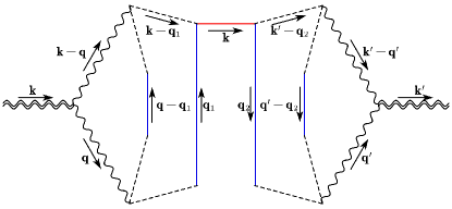
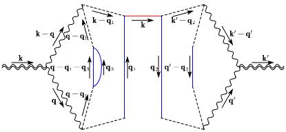
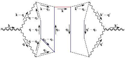
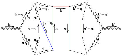
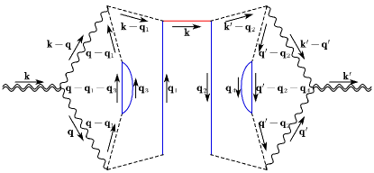
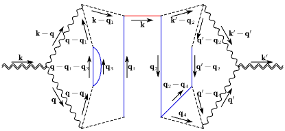
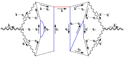
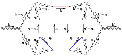
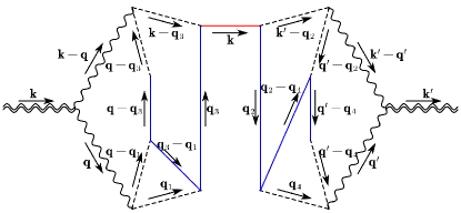
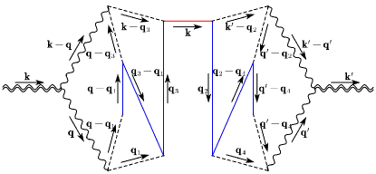
Figure 9: Feynman-like diagrams at $\mathcal{O}(\Delta^{2}_{L})$ order. For brevity, we omit $\lambda$ for the wavy lines.

Following the Feynman-like rules in Fig. 1 and Fig. 8, we can obtain all of the nonvanishing Feynman-like diagrams up to linear order in $\Delta_{L}^{2}$. However, the disconnected diagrams, which are of zeroth order in $\Delta_{L}^{2}$, correspond to the monopole squared, i.e., $\bar{\omega}_{\mathrm{gw}}^{2}(\eta,q)$, which has been studied in Eq. (2.9) and Eq. (4.15). Since they are homogeneous, we disregard them in the following. At linear order in $\Delta_{L}^{2}$, we depict the Feynman-like diagrams in Fig. 9. In each panel of Fig. 9, there is an “$f_{\mathrm{NL}}$ bridge” that connects the initial inhomogeneities at two different locations separated by a long distance. Diagrams at higher order in $\Delta_{L}^{2}$ are negligible due to the assumption of $A_{L}\ll A_{S}$.

The Feynman-like diagrams in Fig. 9 can be understood as follows. On the one hand, there is an ensemble average of the energy density of SIGW over a quantity of Hubble horizons in the neighbourhood of $\mathbf{x}_{\mathrm{in}}$. On the other hand, the energy densities of SIGW at $\mathbf{x}_{\mathrm{in}}$ and $\mathbf{x}_{\mathrm{in}}^{\prime}$ separated by a long distance are connected by the $f_{\mathrm{NL}}$ bridge. Therefore, this picture is equivalent to the following mathematical result

$$\langle\omega_{\mathrm{gw}}(\eta_{\mathrm{in}},\mathbf{x}_{\mathrm{in}},\mathbf{q})\omega_{\mathrm{gw}}(\eta_{\mathrm{in}},\mathbf{x}_{\mathrm{in}}^{\prime},\mathbf{q}^{\prime})\rangle^{\mathcal{O}(\Delta_{L}^{2})}\sim\langle\langle\omega_{\mathrm{gw}}(\eta_{\mathrm{in}},\mathbf{k},\mathbf{q})\rangle_{\mathbf{x}_{\mathrm{in}}}\langle\omega_{\mathrm{gw}}^{\ast}(\eta_{\mathrm{in}},\mathbf{k}^{\prime},\mathbf{q}^{\prime})\rangle_{\mathbf{x}_{\mathrm{in}}^{\prime}}\rangle^{\mathcal{O}(\Delta_{L}^{2})}\ ,$$ (5.6)

where the superscript ${}^{\mathcal{O}(\Delta_{L}^{2})}$ denotes the linear order in $\Delta_{L}^{2}$. During the mathematical derivation, we have approximately take $\mathbf{q}-\mathbf{k}\simeq\mathbf{q}$ because of $k\ll q$. Therefore, the eight-point correlator $\langle\zeta^{8}\rangle$, which is used for expressing $\langle\omega_{\mathrm{gw}}(\eta_{\mathrm{in}},\mathbf{x}_{\mathrm{in}},\mathbf{q})\omega_{\mathrm{gw}}(\eta_{\mathrm{in}},\mathbf{x}_{\mathrm{in}}^{\prime},\mathbf{q}^{\prime})\rangle$, becomes

$$\langle\zeta^{8}\rangle^{\mathcal{O}(\Delta^{2}_{L})}\propto\left(\frac{3}{5}f_{\mathrm{NL}}\right)^{2}\langle\zeta\zeta\zeta\zeta_{S}\rangle_{\mathbf{x}_{\mathrm{in}}}\langle\zeta\zeta\zeta\zeta_{S}\rangle_{\mathbf{x}_{\mathrm{in}}^{\prime}}\int\frac{\mathrm{d}^{3}\mathbf{k}\,\mathrm{d}^{3}\mathbf{k}^{\prime}}{(2\pi)^{3}}e^{i\bigl{(}\mathbf{k}\cdot\mathbf{x}_{\mathrm{in}}-\mathbf{k}^{\prime}\cdot\mathbf{x}_{\mathrm{in}}^{\prime}\bigr{)}}\langle\zeta_{L}(\mathbf{k})\zeta_{L}(-\mathbf{k}^{\prime})\rangle\ .$$ (5.7)

Here, $\langle\zeta\zeta\zeta\zeta_{S}\rangle_{\mathbf{x}_{\mathrm{in}}}$ can be further expressed in terms of the contractions corresponding to the Feynman-like diagrams labeled by $G$, $H$, $C$ and $Z$ in Fig. 2 and Fig. 3.

We provide an explicit formula to Eq. (5.6) in the following. In Fig. 9, we label each diagram with a superscript ^XY if the $f_{\mathrm{NL}}$ bridge connects two sub-diagrams labeled by $X$ and $Y$ corresponding to diagrams in Fig. 2 and Fig. 3. For the top left panel, we have

$$\left\langle\omega_{\mathrm{gw}}(\eta_{\mathrm{in}},\mathbf{x}_{\mathrm{in}},\mathbf{q})\omega_{\mathrm{gw}}(\eta_{\mathrm{in}},\mathbf{x}_{\mathrm{in}}^{\prime},\mathbf{q}^{\prime})\right\rangle^{GG}$$

$$= 2^{6}\Bigl{(}\frac{3}{5}f_{\mathrm{NL}}\Bigr{)}^{2}\bar{\omega}_{\mathrm{gw}}^{G}(\eta_{\mathrm{in}},q)\bar{\omega}_{\mathrm{gw}}^{G}(\eta_{\mathrm{in}},q^{\prime})\int\frac{\mathrm{d}^{3}\mathbf{k}}{(2\pi)^{3}}e^{i\mathbf{k}\cdot(\mathbf{x}_{\mathrm{in}}-\mathbf{x}_{\mathrm{in}}^{\prime})}P_{L}(k)\ ,$$

where the constant $2^{6}$ is an additional symmetric factor due to the $f_{\mathrm{NL}}$ bridge. This diagram has been first evaluated in Ref. [100], but used different convention (the authors of Ref. [100] used $\Gamma$ rather than $\delta\omega_{\mathrm{gw}}$, but the two quantities are related with each other via Eq. (2.22)). Following Ref. [100], the anisotropies in SIGW were further studied in Refs. [101, 103, 94, 104, 106, 102, 105, 107]. For the top right panel, we have

$$\left\langle\omega_{\mathrm{gw}}(\eta_{\mathrm{in}},\mathbf{x}_{\mathrm{in}},\mathbf{q})\omega_{\mathrm{gw}}(\eta_{\mathrm{in}},\mathbf{x}_{\mathrm{in}}^{\prime},\mathbf{q}^{\prime})\right\rangle^{HG+GH}$$

$$= 2^{5}\Bigl{(}\frac{3}{5}f_{\mathrm{NL}}\Bigr{)}^{2}\Bigl{[}\bar{\omega}_{\mathrm{gw}}^{H}(\eta_{\mathrm{in}},q)\bar{\omega}_{\mathrm{gw}}^{G}(\eta_{\mathrm{in}},q^{\prime})+\bar{\omega}_{\mathrm{gw}}^{G}(\eta_{\mathrm{in}},q)\bar{\omega}_{\mathrm{gw}}^{H}(\eta_{\mathrm{in}},q^{\prime})\Bigr{]}\int\frac{\mathrm{d}^{3}\mathbf{k}}{(2\pi)^{3}}e^{i\mathbf{k}\cdot(\mathbf{x}_{\mathrm{in}}-\mathbf{x}_{\mathrm{in}}^{\prime})}P_{L}(k)\ ,$$

where the constant $2^{5}$ is also an symmetric factor. The expressions for the diagrams in other panels can also be obtained in the same way, but the corresponding derivation processes have been neglected here. Summing these results, we eventually get the formula as follows

$$\left\langle\omega_{\mathrm{gw}}(\eta_{\mathrm{in}},\mathbf{x}_{\mathrm{in}},\mathbf{q})\omega_{\mathrm{gw}}(\eta_{\mathrm{in}},\mathbf{x}_{\mathrm{in}}^{\prime},\mathbf{q}^{\prime})\right\rangle^{\mathcal{O}(\Delta^{2}_{L})}$$

$$= \frac{\Omega_{\mathrm{ng}}(\eta_{\mathrm{in}},q)}{4\pi}\frac{\Omega_{\mathrm{ng}}(\eta_{\mathrm{in}},q’)}{4\pi}\left(\frac{3}{5}f_{\mathrm{NL}}\right)^{2}\int\frac{\mathrm{d}^{3}\mathbf{k}}{(2\pi)^{3}}e^{i\mathbf{k}\cdot(\mathbf{x}_{\mathrm{in}}-\mathbf{x}_{\mathrm{in}}^{\prime})}P_{L}(k)\ ,$$

where we introduce a new quantity $\Omega_{\mathrm{ng}}$ for concision, defined as

$$\Omega_{\mathrm{ng}}(\eta_{\mathrm{in}},q)=2^{3}\bar{\Omega}_{\mathrm{gw}}^{G}(\eta_{\mathrm{in}},q)+2^{2}\bar{\Omega}_{\mathrm{gw}}^{H}(\eta_{\mathrm{in}},q)+2^{2}\bar{\Omega}_{\mathrm{gw}}^{C}(\eta_{\mathrm{in}},q)+2^{2}\bar{\Omega}_{\mathrm{gw}}^{Z}(\eta_{\mathrm{in}},q)\ .$$ (5.11)

To simplify computation in the following, we equivalently express the initial inhomogeneities $\delta\omega_{\mathrm{gw}}(\eta_{\mathrm{in}},\mathbf{x}_{\mathrm{in}},\mathbf{q})$ as follows

$$\delta\omega_{\mathrm{gw}}(\eta_{\mathrm{in}},\mathbf{x}_{\mathrm{in}},\mathbf{q})=\frac{\Omega_{\mathrm{ng}}(\eta_{\mathrm{in}},q)}{4\pi}\left(\frac{3}{5}f_{\mathrm{NL}}\right)\int\frac{\mathrm{d}^{3}\mathbf{k}}{(2\pi)^{3/2}}e^{i\mathbf{k}\cdot\mathbf{x}_{\mathrm{in}}}\zeta_{L}(\mathbf{k})\ ,$$ (5.12)

which can reproduce Eq. (5.1.2). Based on Eq. 2.12, $\delta\omega_{\mathrm{gw}}(\eta_{\mathrm{in}},\mathbf{x}_{\mathrm{in}},\mathbf{q})$ can be further transformed into the initial density contrast as

$$\delta_{\mathrm{gw}}(\eta_{\mathrm{in}},\mathbf{x}_{\mathrm{in}},\mathbf{q})=\left(\frac{3}{5}f_{\mathrm{NL}}\right)\frac{\Omega_{\mathrm{ng}}(\eta_{\mathrm{in}},q)}{\bar{\Omega}_{\mathrm{gw}}(\eta_{\mathrm{in}},q)}\int\frac{\mathrm{d}^{3}\mathbf{k}}{(2\pi)^{3/2}}e^{i\mathbf{k}\cdot\mathbf{x}_{\mathrm{in}}}\zeta_{L}(\mathbf{k})\ ,$$ (5.13)

which will be used for computation of the angular power spectrum in the next subsection. The factor $\Omega_{\mathrm{ng}}/\bar{\Omega}_{\mathrm{gw}}$ would be replaced by a constant in the previous work [100], but depends on GW frequency in our current work.

5.1.3 Two-point angular correlation functions

Substituting Eq. 5.13 and Eq. 5.4 into Eq. (5.3), we have the observed density contrast

$$\delta_{\mathrm{gw}}(\mathbf{q})=\frac{3}{5}\Biggl{\{}f_{\mathrm{NL}}\frac{\Omega_{\mathrm{ng}}(\eta_{\mathrm{in}},q)}{\bar{\Omega}_{\mathrm{gw}}(\eta_{\mathrm{in}},q)}+[4-n_{\mathrm{gw}}(q)]\Biggr{\}}\int\frac{\mathrm{d}^{3}\mathbf{k}}{(2\pi)^{3/2}}e^{i\mathbf{k}\cdot\mathbf{x}_{\mathrm{in}}}\zeta_{L}(\mathbf{k})\ .$$ (5.14)

We can express $\langle\delta_{\mathrm{gw}}(\mathbf{q})\delta_{\mathrm{gw}}(\mathbf{q}^{\prime})\rangle$ in terms of the two-point correlator of $\zeta_{L}$, defined in Eq. 5.2a. Assuming $\Delta_{L}^{2}(k)$ to be scale-invariant, we analytically calculate the following integral

$$\int\frac{\mathrm{d}^{3}\mathbf{k}\,\mathrm{d}^{3}\mathbf{k}^{\prime}}{(2\pi)^{3}}e^{i\left(\mathbf{k}\cdot\mathbf{x}_{\mathrm{in}}-\mathbf{k}^{\prime}\cdot\mathbf{x}_{\mathrm{in}}^{\prime}\right)}\langle\zeta_{L}(\mathbf{k})\zeta_{L}(-\mathbf{k}^{\prime})\rangle = 4\pi\Delta^{2}_{L}\sum_{\ell m}Y_{\ell m}(\mathbf{n}_{0})Y^{\ast}_{\ell m}(\mathbf{n}_{0}^{\prime})\int\mathrm{d}\ln k\,j_{\ell}^{2}[k\left(\eta_{0}-\eta_{\mathrm{in}}\right)]$$ (5.15)

$$\simeq \sum_{\ell m}Y_{\ell m}(\mathbf{n}_{0})Y^{\ast}_{\ell m}(\mathbf{n}_{0}^{\prime})\frac{2\pi}{\ell(\ell+1)}\times\Delta_{L}^{2}\ ,$$

where we use a relation of $\mathbf{x}_{\mathrm{in}}-\mathbf{x}_{\mathrm{in}}^{\prime}=(\eta_{\mathrm{in}}-\eta_{0})(\mathbf{n}_{0}-\mathbf{n}_{0}^{\prime})$, the identity of the form $e^{ik\mu(\eta_{\mathrm{in}}-\eta_{0})}=4\pi\sum_{\ell m}(-i)^{\ell}j_{\ell}[k(\eta_{0}-\eta_{\mathrm{in}})]Y^{\ast}_{\ell m}(\hat{k})Y_{\ell m}(\mathbf{n}_{0})$, and the integral $\int\mathrm{d}\ln k\,j_{\ell}^{2}[k\left(\eta_{0}-\eta_{\mathrm{in}}\right)]=1/[2\ell(\ell+1)]$ due to $\eta_{0}\gg\eta_{\mathrm{in}}$. Eventually, combining Eq. 2.14, Eq. 5.14, and Eq. (5.15), we obtain the reduced angular power spectrum defined in Eq. 2.15, i.e.,

$$\widetilde{C}_{\ell}(q,q^{\prime})= \frac{18\pi\Delta^{2}_{L}}{25\ell(\ell+1)}\times\biggl{[}f_{\mathrm{NL}}\frac{\Omega_{\mathrm{ng}}(\eta_{\mathrm{in}},q)}{\bar{\Omega}_{\mathrm{gw}}(\eta_{\mathrm{in}},q)}+\bigl{(}4-n_{\mathrm{gw}}(q)\bigr{)}\biggr{]}$$ (5.16)

$$\hphantom{\frac{18\pi\Delta^{2}_{L}}{25\ell(\ell+1)}}\times\biggl{[}f_{\mathrm{NL}}\frac{\Omega_{\mathrm{ng}}(\eta_{\mathrm{in}},q^{\prime})}{\bar{\Omega}_{\mathrm{gw}}(\eta_{\mathrm{in}},q^{\prime})}+\bigl{(}4-n_{\mathrm{gw}}(q^{\prime})\bigr{)}\biggr{]}\ .$$

Correspondingly, the angular power spectrum defined in Eq. 2.16 is given as

$$C_{\ell}(q,q^{\prime}) = \frac{9\Delta^{2}_{L}\bar{\Omega}_{\mathrm{gw}}(q)\bar{\Omega}_{\mathrm{gw}}(q^{\prime})}{200\pi\ell(\ell+1)}\times\biggl{[}f_{\mathrm{NL}}\frac{\Omega_{\mathrm{ng}}(\eta_{\mathrm{in}},q)}{\bar{\Omega}_{\mathrm{gw}}(\eta_{\mathrm{in}},q)}+\bigl{(}4-n_{\mathrm{gw}}(q)\bigr{)}\biggr{]}$$ (5.17)

$$\hphantom{\frac{9\Delta^{2}_{L}\bar{\Omega}_{\mathrm{gw}}(q)\bar{\Omega}_{\mathrm{gw}}(q^{\prime})}{200\pi\ell(\ell+1)}}\times\biggl{[}f_{\mathrm{NL}}\frac{\Omega_{\mathrm{ng}}(\eta_{\mathrm{in}},q^{\prime})}{\bar{\Omega}_{\mathrm{gw}}(\eta_{\mathrm{in}},q^{\prime})}+\bigl{(}4-n_{\mathrm{gw}}(q^{\prime})\bigr{)}\biggr{]}\ .$$

This is the most important formula of this paper. Besides the radiation domination, it is so generic that also available during other epochs. Eq. (5.17) indicates that the angular power spectrum of SIGW consists of the initial inhomogeneities, the SW effect, and the cross terms between them. We will evaluate it numerically in the following subsection.

In Eq. (5.16), the initial inhomogeneities are explicitly determined by the parameter $f_{\mathrm{NL}}$ as well as the parameter $A_{S}f_{\mathrm{NL}}^{2}$ in $\Omega_{\mathrm{ng}}/\bar{\Omega}_{\mathrm{gw}}$ (besides $\sigma$ and $q_{\ast}$), indicating that the sign degeneracy in $f_{\mathrm{NL}}$ is explicitly broken. In contrast, the SW effect is determined by $A_{S}f_{\mathrm{NL}}^{2}$ only (besides $\sigma$ and $q_{\ast}$). These results would lead to interesting theoretical expectations in the next subsection. In fact, a ratio between the cross terms that are linear in $f_{\mathrm{NL}}$ and the $f_{\mathrm{NL}}^{2}$ term is roughly proportional to $2(4-n_{\mathrm{gw}})/(f_{\mathrm{NL}}\Omega_{\mathrm{ng}}/\bar{\Omega}_{\mathrm{gw}})$. Since $n_{\mathrm{gw}}\sim\mathcal{O}(1)$ and $\Omega_{\mathrm{ng}}/\bar{\Omega}_{\mathrm{gw}}\sim\mathcal{O}(1)$, we have possibilities to get the largest breaking of the sign degeneracy of $f_{\mathrm{NL}}$ when we concern $f_{\mathrm{NL}}\sim\mathcal{O}(1)$. In other words, to get the largest breaking of the sign degeneracy of $f_{\mathrm{NL}}$, we require an approximate balance between the $f_{\mathrm{NL}}$ terms and the $n_{\mathrm{gw}}$ term, making the cross terms to be roughly equal to other terms, or at least the same order of magnitude. To further demonstrate the above issue, we will show some numerical results in the next subsection.

The (reduced) angular power spectrum has multipole dependence and frequency dependence. On the one hand, the multiple dependence, i.e., $C_{\ell}\propto[\ell(\ell+1)]^{-1}$, might be vital for discrimination of SIGW from other GW sources, e.g., astrophysical foregrounds due to GW emitted from BBH [128, 129, 130] and topological defects such as cosmic string loops [131, 94]. For example, in the LISA band, the angular power spectrum for inspiralling BBH has been shown to roughly scale as $(\ell+1/2)^{-1}$ [128, 129]. As a second example, the angular power spectrum for cosmic string loops has been shown to be spectrally white, i.e., $C_{\ell}\propto\ell^{0}$ [131, 94]. On the other hand, Eq. (5.16) depends on the GW frequency band due to a factor $\Omega_{\mathrm{ng}}/\bar{\Omega}_{\mathrm{gw}}$ in the $f_{\mathrm{NL}}$ term. Via the component separation approach, the frequency dependence may be useful for discriminating SIGW from other CGWB produced by, e.g., the first-order phase transitions in the early universe [132, 133, 94, 134, 103].

5.2 Numerical results

In this subsection, we straightforwardly compute Eq. (5.16) and Eq. (5.17) by utilizing the results of $\bar{\Omega}_{\mathrm{gw}}^{X}$ obtained in Section 4, where $X=G,H,C,Z,R,P$ and $N$.

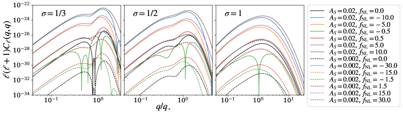
Figure 10: Angular power spectrum for the anisotropies in SIGW. The spectra with $A_{S}=0.02$ are denoted by solid curves, and the spectra with $A_{S}=0.002$ are denoted by dashed curves. We take $\sigma=1/3,~{}1/2,~{}1$ from left to right panels.

In Fig. 10, we show the (auto-correlated) angular power spectrum $\ell(\ell+1)C_{\ell}$ at the same frequency band, i.e., $q^{\prime}=q$. First of all, the sign degeneracy of $f_{\mathrm{NL}}$ is broken obviously in the figure. This result can be interpreted by the cross terms in Eq. (5.17), because they are linear in $f_{\mathrm{NL}}$. In particular, the difference in two spectra with $\pm|f_{\mathrm{NL}}|$ is relatively more significant, when the $f_{\mathrm{NL}}$ term is comparable with the SW term in Eq. (5.17). In addition, we find that $C_{\ell}$ further depends on $A_{S}$ and $\sigma$. Particularly, it roughly scales in $A_{S}^{4}$ since $C_{\ell}$ is approximately proportional to $\bar{\Omega}_{\mathrm{gw}}^{2}$ in Eq. (5.17).

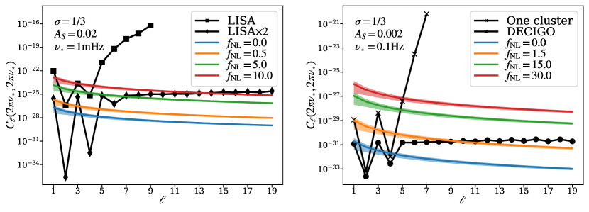
Figure 11: The anticipated angular power spectra versus the noise angular power spectra of LISA (at 1 mHz band, left panel) [135] and DECIGO (at 0.1 Hz band, right panel) [135]. The shaded regions stand for the cosmic-variance limits (68% confidence level).

As is shown in Fig. 11, the angular power spectra with the interested parameter regimes are potentially detectable for LISA [136] and DECIGO [137, 138], particularly on low multipoles. For comparison, we plot the shaded regions to stand for the uncertainties at 68% confidence level due to cosmic variance, which is given as

$$\frac{\Delta C_{\ell}}{C_{\ell}}=\sqrt{\frac{2}{2\ell+1}}\ .$$ (5.18)

A detector network could measure the angular power spectrum for multipoles $\ell=1-19$ with a significantly higher sensitivity than an individual cluster [135]. This result may also bring new insights to potential developments of the LISA-Taiji network [139, 140].

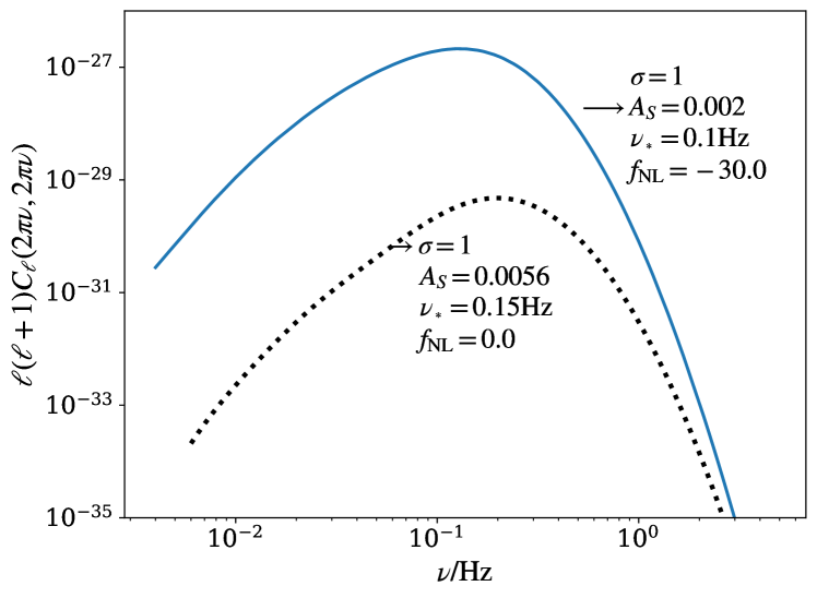
Figure 12: Illustration of the broken degeneracy of model parameters via the angular power spectrum. The degeneracy has been shown in Fig. 7 for the energy-density fraction spectrum.

In Fig. 12, we show that the degeneracies of model parameters, as have been mentioned in Fig. 7, could be explicitly broken by using the angular power spectrum. To be specific, corresponding to two curves in Fig. 12, the two curves with the same labeling in Fig. 7 almost coincides with each other, indicating degeneracies in these two sets of parameters. However, in Fig. 12, the degeneracies disappear due to an obvious separation of the two curves, with difference of at least two orders of magnitude.

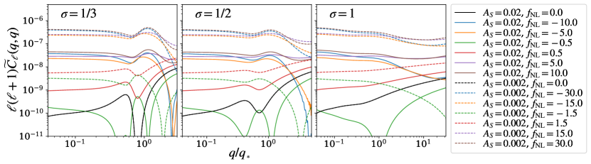
Figure 13: Reduced angular power spectrum as well as its dependence on $f_{\mathrm{NL}}$ and $A_{S}$, and $\sigma$. The labeling is the same as that of Fig. 10.

In Fig. 13, we depict the reduced angular power spectrum to display the difference in parameter dependence between the monopole and multipoles. Firstly, the magnitude of $\tilde{C}_{\ell}$ decreases with increase of $A_{S}$, implying that $C_{\ell}$ is less dependent on $A_{S}$ than $\bar{\Omega}_{\mathrm{gw}}$. Secondly, $\tilde{C}_{\ell}$ is roughly red-tilted for a large value of $|f_{\mathrm{NL}}|$, while blue-tilted for a small value. The critical value is roughly determined by a balance between the $f_{\mathrm{NL}}$ term and the SW term. Thirdly, the profiles of $\tilde{C}_{\ell}$ also vary with values of $\sigma$, implying that $C_{\ell}$ and $\bar{\Omega}_{\mathrm{gw}}$ have different dependence on $\sigma$. The above theoretical expectations are potentially useful for breaking the degeneracies of model parameters.

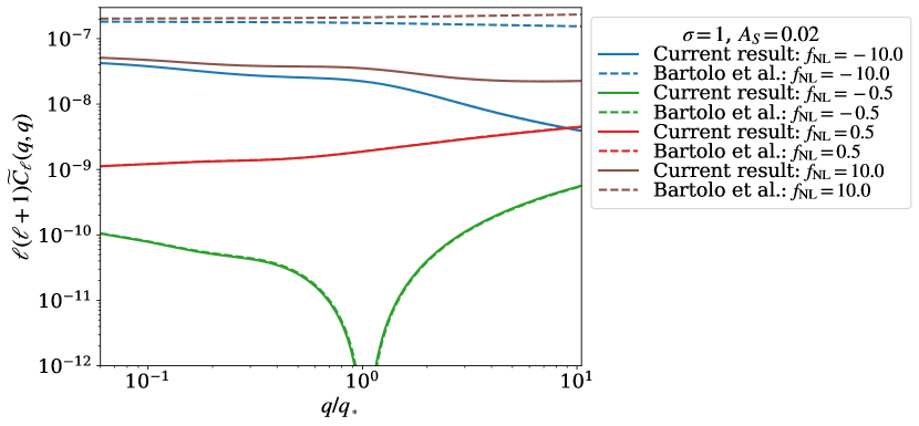
Figure 14: Comparison of the reduced angular power spectra of SIGW provided by the current work (solid curves) and Ref. [100] (dashed curves).

In Fig. 14, we show the results for the reduced angular power spectra anticipated by our current work and then compare them with those of Ref. [100]. Regarding the frequency dependence, we find that difference between the reduced angular power spectra of the two works is larger, when $|f_{\mathrm{NL}}|$ takes a larger value, given a value of $A_{S}$. This result implies more significant impacts on the anisotropies in SIGW with the increase of $|f_{\mathrm{NL}}|$, or more precisely, the combination $A_{S}f_{\mathrm{NL}}^{2}$. In particular, we find that the difference could be one order of magnitude for a large non-Gaussianity. This result can be interpreted as follows. On the level of background, i.e., $\bar{\Omega}_{\mathrm{gw}}$, the authors of Ref. [100] considered only the left panel of Fig. 2, implying . In contrast, besides this diagram, we take into account the other six diagrams in Fig. 3. On the level of fluctuations, only one Feynman-like diagram, i.e., the top left panel of Fig. 9, was taken into account in Ref. [98]. It was shown that the frequency dependence of $\tilde{C}_{\ell}$ arises from the $n_{\mathrm{gw}}(q)$ term. In contrast, we take into account all of the ten Feynman-like diagrams in Fig. 9. We show that the frequency dependence of $\tilde{C}_{\ell}$ arises not only from $n_{\mathrm{gw}}(q)$, but also from the $f_{\mathrm{NL}}$ term that is now multiplied with a frequency-dependent function of the form $\Omega_{\mathrm{ng}}/\bar{\Omega}_{\mathrm{GW}}$. In summary, the above two ingredients lead to the main difference between our current work and Ref. [98].

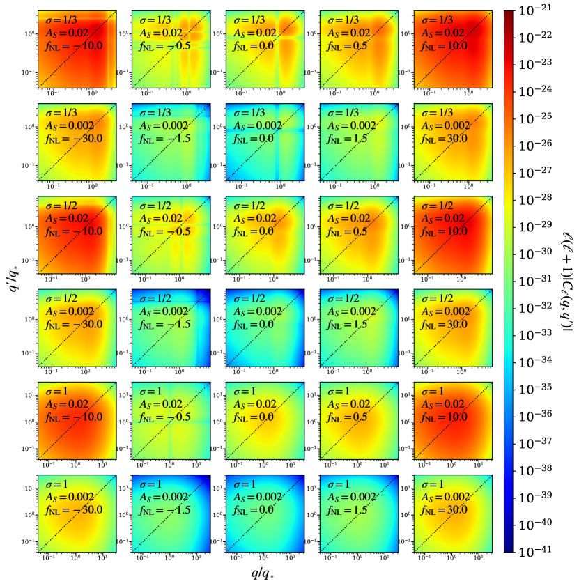
Figure 15: Cross-correlated angular power spectrum with respect to the gravitational-wave frequency band. In each panel, the dotted line refers to the auto-correlated angular power spectrum.

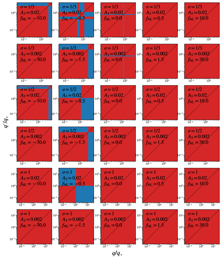
Figure 16: The same as Fig. 15, but the correlation factor is shown in red color for $r_{\ell}(q,q^{\prime})=+1$ while in blue color for $r_{\ell}(q,q^{\prime})=-1$.

In Fig. 15, we depict the (cross-correlated) angular power spectra $\ell(\ell+1)|C_{\ell}|$ at different frequency bands, i.e., $q^{\prime}\neq q$. Here, hotter colors stand for larger correlations while colder ones denote smaller correlations. For comparison, the auto-correlated spectra are also depicted in dotted black lines. The cross-correlation might be available to mitigate the stochastic noise that diminishes the anticipated signal. A correlation factor is defined as [103]

$$r_{\ell}(q,q^{\prime})=\frac{C_{\ell}(q,q^{\prime})}{\sqrt{C_{\ell}(q,q)C_{\ell}(q^{\prime},q^{\prime})}}\ .$$ (5.19)

Considering Eq. (5.17), we obtain $r_{\ell}(q,q^{\prime})=\pm 1$. Note that we always have $r_{\ell}(q,q)=+1$. As is shown in Fig. 16, the changes of the sign depend on the value of the pair $(q,q^{\prime})$, indicating that SIGW encode information in it. Therefore, only the sign is important, rather than $C_{\ell}(q,q^{\prime})$ itself. In contrast, the noise may have different cross-correlation from the signal. If so, the cross-correlation would be useful for differentiating the signal from the noise. Note that this prediction is to some extent speculative. However, we would like to point out such a possibility, which may be useful to future related studies. In Fig. 15, we still depict the absolute value of $C_{\ell}(q,q^{\prime})$, with dotted lines standing for the auto-correlated spectra. However, $r_{\ell}(q,q^{\prime})$ could be straightforwardly computed in practice.

6 Conclusion

In this work, we proposed the anisotropies in SIGW as a powerful probe to the local-type PNG in the cosmological curvature perturbations. For the energy-density fraction spectrum of SIGW, we reproduced the existing results in the literature and showed the degeneracies between the non-Gaussian parameter and other model parameters, that bring challenges to determination of the PNG. For the first time, we provided the complete analysis to the (reduced) angular power spectrum of anisotropies in SIGW, particularly, the contributions from the PNG. In Eq. (5.16), we showed that such a spectrum is explicitly determined by $f_{\mathrm{NL}}$, $A_{S}f_{\mathrm{NL}}^{2}$, $\sigma$, and $q_{\ast}$, indicating that the degeneracies of model parameters can be broken. The spectrum was also shown to have multipole dependence, i.e., $C_{\ell}\sim[\ell(\ell+1)]^{-1}$, and be dependent on GW frequency. In particular, the initial inhomogeneities were shown to be dependent on GW frequency. These properties may be useful for the component separation and foreground removal. Despite challenges for breaking the sign degeneracy of $f_{\mathrm{NL}}$ in the angular power spectrum for large $|f_{\mathrm{NL}}|$, probing PBH may provide a promising way to further break this degeneracy. The presence of primordial non-Gaussianity has substantial impacts on the abundance and mass distribution of PBH, as their formation threshold is influenced by levels of this non-Gaussianity [81, 82, 48, 100, 86, 141, 142]. Notably, a sizable negative $f_{\mathrm{NL}}$ would be incompatible with detection of PBH [81, 82], since the abundance of PBH is expected to be suppressed significantly. Conversely, it is expected that a sizable positive $f_{\mathrm{NL}}$ could significantly enhance the abundance of PBH. Therefore, measuring the anisotropies in SIGW and probing PBH can serve as complementary approaches to break the sign degeneracy of $f_{\mathrm{NL}}$. In addition, the theoretical formalism could be straightforwardly generalized to study SIGW produced during other epochs [143] or other CGWB. The theoretical predictions of this work may be tested by space-borne GW detectors or networks in future.

References

- [1] J.M. Maldacena, Non-Gaussian features of primordial fluctuations in single field inflationary models, JHEP 05 (2003) 013 [astro-ph/0210603].
- [2] N. Bartolo, E. Komatsu, S. Matarrese and A. Riotto, Non-Gaussianity from inflation: Theory and observations, Phys. Rept. 402 (2004) 103 [astro-ph/0406398].
- [3] T.J. Allen, B. Grinstein and M.B. Wise, Nongaussian Density Perturbations in Inflationary Cosmologies, Phys. Lett. B 197 (1987) 66.
- [4] N. Bartolo, S. Matarrese and A. Riotto, Nongaussianity from inflation, Phys. Rev. D 65 (2002) 103505 [hep-ph/0112261].
- [5] V. Acquaviva, N. Bartolo, S. Matarrese and A. Riotto, Second order cosmological perturbations from inflation, Nucl. Phys. B 667 (2003) 119 [astro-ph/0209156].
- [6] F. Bernardeau and J.-P. Uzan, NonGaussianity in multifield inflation, Phys. Rev. D 66 (2002) 103506 [hep-ph/0207295].
- [7] X. Chen, M.-x. Huang, S. Kachru and G. Shiu, Observational signatures and non-Gaussianities of general single field inflation, JCAP 01 (2007) 002 [hep-th/0605045].
- [8] P.D. Meerburg et al., Primordial Non-Gaussianity, 1903.04409.
- [9] D.H. Lyth, C. Ungarelli and D. Wands, The Primordial density perturbation in the curvaton scenario, Phys. Rev. D 67 (2003) 023503 [astro-ph/0208055].
- [10] N. Bartolo, S. Matarrese and A. Riotto, On nonGaussianity in the curvaton scenario, Phys. Rev. D 69 (2004) 043503 [hep-ph/0309033].
- [11] M. Zaldarriaga, Non-Gaussianities in models with a varying inflaton decay rate, Phys. Rev. D 69 (2004) 043508 [astro-ph/0306006].
- [12] D.H. Lyth, Generating the curvature perturbation at the end of inflation, JCAP 11 (2005) 006 [astro-ph/0510443].
- [13] A. Linde, S. Mooij and E. Pajer, Gauge field production in supergravity inflation: Local non-Gaussianity and primordial black holes, Phys. Rev. D 87 (2013) 103506 [1212.1693].
- [14] J. Torrado, C.T. Byrnes, R.J. Hardwick, V. Vennin and D. Wands, Measuring the duration of inflation with the curvaton, Phys. Rev. D 98 (2018) 063525 [1712.05364].
- [15] J. Frazer and A.R. Liddle, Multi-field inflation with random potentials: field dimension, feature scale and non-Gaussianity, JCAP 02 (2012) 039 [1111.6646].
- [16] L. McAllister, S. Renaux-Petel and G. Xu, A Statistical Approach to Multifield Inflation: Many-field Perturbations Beyond Slow Roll, JCAP 10 (2012) 046 [1207.0317].
- [17] T. Bjorkmo and M.C.D. Marsh, Manyfield Inflation in Random Potentials, JCAP 02 (2018) 037 [1709.10076].
- [18] M.H. Namjoo, H. Firouzjahi and M. Sasaki, Violation of non-Gaussianity consistency relation in a single field inflationary model, EPL 101 (2013) 39001 [1210.3692].
- [19] J. Martin, H. Motohashi and T. Suyama, Ultra Slow-Roll Inflation and the non-Gaussianity Consistency Relation, Phys. Rev. D 87 (2013) 023514 [1211.0083].
- [20] X. Chen, H. Firouzjahi, M.H. Namjoo and M. Sasaki, A Single Field Inflation Model with Large Local Non-Gaussianity, EPL 102 (2013) 59001 [1301.5699].
- [21] Q.-G. Huang and Y. Wang, Large Local Non-Gaussianity from General Single-field Inflation, JCAP 06 (2013) 035 [1303.4526].
- [22] S. Mooij and G.A. Palma, Consistently violating the non-Gaussian consistency relation, JCAP 11 (2015) 025 [1502.03458].
- [23] R. Bravo, S. Mooij, G.A. Palma and B. Pradenas, A generalized non-Gaussian consistency relation for single field inflation, JCAP 05 (2018) 024 [1711.02680].
- [24] B. Finelli, G. Goon, E. Pajer and L. Santoni, Soft Theorems For Shift-Symmetric Cosmologies, Phys. Rev. D 97 (2018) 063531 [1711.03737].
- [25] Y.-F. Cai, X. Chen, M.H. Namjoo, M. Sasaki, D.-G. Wang and Z. Wang, Revisiting non-Gaussianity from non-attractor inflation models, JCAP 05 (2018) 012 [1712.09998].
- [26] S. Passaglia, W. Hu and H. Motohashi, Primordial black holes and local non-Gaussianity in canonical inflation, Phys. Rev. D 99 (2019) 043536 [1812.08243].
- [27] Planck collaboration, Planck 2018 results. IX. Constraints on primordial non-Gaussianity, Astron. Astrophys. 641 (2020) A9 [1905.05697].
- [28] V.F. Mukhanov and G.V. Chibisov, Quantum Fluctuations and a Nonsingular Universe, JETP Lett. 33 (1981) 532.
- [29] J. Chluba, J. Hamann and S.P. Patil, Features and New Physical Scales in Primordial Observables: Theory and Observation, Int. J. Mod. Phys. D 24 (2015) 1530023 [1505.01834].
- [30] A. Rotti, A. Ravenni and J. Chluba, Non-Gaussianity constraints with anisotropic distortion measurements from Planck, Mon. Not. Roy. Astron. Soc. 515 (2022) 5847 [2205.15971].
- [31] C. Stahl, T. Montandon, B. Famaey, O. Hahn and R. Ibata, Exploring the effects of primordial non-Gaussianity at galactic scales, 2209.15038.
- [32] N. Sabti, J.B. Muñoz and D. Blas, First Constraints on Small-Scale Non-Gaussianity from UV Galaxy Luminosity Functions, JCAP 01 (2021) 010 [2009.01245].
- [33] S. Dodelson, Modern Cosmology, Academic Press, Amsterdam (2003).
- [34] M. Maggiore, Gravitational wave experiments and early universe cosmology, Phys. Rept. 331 (2000) 283 [gr-qc/9909001].
- [35] K. Inomata and T. Nakama, Gravitational waves induced by scalar perturbations as probes of the small-scale primordial spectrum, Phys. Rev. D 99 (2019) 043511 [1812.00674].
- [36] F. Hajkarim and J. Schaffner-Bielich, Thermal History of the Early Universe and Primordial Gravitational Waves from Induced Scalar Perturbations, Phys. Rev. D 101 (2020) 043522 [1910.12357].
- [37] G. Domènech, S. Pi and M. Sasaki, Induced gravitational waves as a probe of thermal history of the universe, JCAP 08 (2020) 017 [2005.12314].
- [38] Y.-H. Yu and S. Wang, Primordial Gravitational Waves Assisted by Cosmological Scalar Perturbations, 2303.03897.
- [39] X. Zhang, J.-Z. Zhou and Z. Chang, Impact of the free-streaming neutrinos to the second order induced gravitational waves, Eur. Phys. J. C 82 (2022) 781 [2208.12948].
- [40] Z. Chang, X. Zhang and J.-Z. Zhou, Gravitational waves from primordial scalar and tensor perturbations, Phys. Rev. D 107 (2023) 063510 [2209.07693].
- [41] Z. Chang, S. Wang and Q.-H. Zhu, Note on gauge invariance of second order cosmological perturbations, Chin. Phys. C 45 (2021) 095101 [2009.11025].
- [42] K. Inomata, K. Kohri, T. Nakama and T. Terada, Enhancement of Gravitational Waves Induced by Scalar Perturbations due to a Sudden Transition from an Early Matter Era to the Radiation Era, Phys. Rev. D 100 (2019) 043532 [1904.12879].
- [43] K. Inomata, K. Kohri, T. Nakama and T. Terada, Gravitational Waves Induced by Scalar Perturbations during a Gradual Transition from an Early Matter Era to the Radiation Era, JCAP 10 (2019) 071 [1904.12878].
- [44] N. Bartolo, A. Hoseinpour, G. Orlando, S. Matarrese and M. Zarei, Photon-graviton scattering: A new way to detect anisotropic gravitational waves?, Phys. Rev. D 98 (2018) 023518 [1804.06298].
- [45] R. Flauger and S. Weinberg, Absorption of Gravitational Waves from Distant Sources, Phys. Rev. D 99 (2019) 123030 [1906.04853].
- [46] J. Garcia-Bellido, M. Peloso and C. Unal, Gravitational Wave signatures of inflationary models from Primordial Black Hole Dark Matter, JCAP 09 (2017) 013 [1707.02441].
- [47] G. Domènech and M. Sasaki, Hamiltonian approach to second order gauge invariant cosmological perturbations, Phys. Rev. D 97 (2018) 023521 [1709.09804].
- [48] T. Nakama, J. Silk and M. Kamionkowski, Stochastic gravitational waves associated with the formation of primordial black holes, Phys. Rev. D 95 (2017) 043511 [1612.06264].
- [49] R.-g. Cai, S. Pi and M. Sasaki, Gravitational Waves Induced by non-Gaussian Scalar Perturbations, Phys. Rev. Lett. 122 (2019) 201101 [1810.11000].
- [50] C. Unal, Imprints of Primordial Non-Gaussianity on Gravitational Wave Spectrum, Phys. Rev. D 99 (2019) 041301 [1811.09151].
- [51] C. Yuan and Q.-G. Huang, Gravitational waves induced by the local-type non-Gaussian curvature perturbations, Phys. Lett. B 821 (2021) 136606 [2007.10686].
- [52] V. Atal and G. Domènech, Probing non-Gaussianities with the high frequency tail of induced gravitational waves, JCAP 06 (2021) 001 [2103.01056].
- [53] P. Adshead, K.D. Lozanov and Z.J. Weiner, Non-Gaussianity and the induced gravitational wave background, JCAP 10 (2021) 080 [2105.01659].
- [54] H.V. Ragavendra, Accounting for scalar non-Gaussianity in secondary gravitational waves, Phys. Rev. D 105 (2022) 063533 [2108.04193].
- [55] K.N. Ananda, C. Clarkson and D. Wands, The Cosmological gravitational wave background from primordial density perturbations, Phys. Rev. D 75 (2007) 123518 [gr-qc/0612013].
- [56] D. Baumann, P.J. Steinhardt, K. Takahashi and K. Ichiki, Gravitational Wave Spectrum Induced by Primordial Scalar Perturbations, Phys. Rev. D 76 (2007) 084019 [hep-th/0703290].
- [57] S. Mollerach, D. Harari and S. Matarrese, CMB polarization from secondary vector and tensor modes, Phys. Rev. D 69 (2004) 063002 [astro-ph/0310711].
- [58] H. Assadullahi and D. Wands, Constraints on primordial density perturbations from induced gravitational waves, Phys. Rev. D 81 (2010) 023527 [0907.4073].
- [59] J.R. Espinosa, D. Racco and A. Riotto, A Cosmological Signature of the SM Higgs Instability: Gravitational Waves, JCAP 09 (2018) 012 [1804.07732].
- [60] K. Kohri and T. Terada, Semianalytic calculation of gravitational wave spectrum nonlinearly induced from primordial curvature perturbations, Phys. Rev. D 97 (2018) 123532 [1804.08577].
- [61] V. Atal, J. Garriga and A. Marcos-Caballero, Primordial black hole formation with non-Gaussian curvature perturbations, JCAP 09 (2019) 073 [1905.13202].
- [62] S.S. Mishra and V. Sahni, Primordial Black Holes from a tiny bump/dip in the Inflaton potential, JCAP 04 (2020) 007 [1911.00057].
- [63] J.M. Ezquiaga, J. Garcia-Bellido and E. Ruiz Morales, Primordial Black Hole production in Critical Higgs Inflation, Phys. Lett. B 776 (2018) 345 [1705.04861].
- [64] F. Bezrukov, M. Pauly and J. Rubio, On the robustness of the primordial power spectrum in renormalized Higgs inflation, JCAP 02 (2018) 040 [1706.05007].
- [65] M. Drees and Y. Xu, Overshooting, Critical Higgs Inflation and Second Order Gravitational Wave Signatures, Eur. Phys. J. C 81 (2021) 182 [1905.13581].
- [66] NANOGrav collaboration, The NANOGrav 12.5 yr Data Set: Search for an Isotropic Stochastic Gravitational-wave Background, Astrophys. J. Lett. 905 (2020) L34 [2009.04496].
- [67] V. De Luca, G. Franciolini and A. Riotto, NANOGrav Data Hints at Primordial Black Holes as Dark Matter, Phys. Rev. Lett. 126 (2021) 041303 [2009.08268].
- [68] V. Vaskonen and H. Veermäe, Did NANOGrav see a signal from primordial black hole formation?, Phys. Rev. Lett. 126 (2021) 051303 [2009.07832].
- [69] K. Kohri and T. Terada, Solar-Mass Primordial Black Holes Explain NANOGrav Hint of Gravitational Waves, Phys. Lett. B 813 (2021) 136040 [2009.11853].
- [70] G. Domènech and S. Pi, NANOGrav hints on planet-mass primordial black holes, Sci. China Phys. Mech. Astron. 65 (2022) 230411 [2010.03976].
- [71] V. Atal, A. Sanglas and N. Triantafyllou, NANOGrav signal as mergers of Stupendously Large Primordial Black Holes, JCAP 06 (2021) 022 [2012.14721].
- [72] Z. Yi and Q. Fei, Constraints on primordial curvature spectrum from primordial black holes and scalar-induced gravitational waves, Eur. Phys. J. C 83 (2023) 82 [2210.03641].
- [73] Z.-C. Zhao and S. Wang, Bayesian Implications for the Primordial Black Holes from ’NANOGravs Pulsar-Timing Data Using the Scalar-Induced Gravitational Waves, Universe 9 (2023) 157 [2211.09450].
- [74] V. Dandoy, V. Domcke and F. Rompineve, Search for scalar induced gravitational waves in the International Pulsar Timing Array Data Release 2 and NANOgrav 12.5 years dataset, 2302.07901.
- [75] R.-G. Cai, C. Chen and C. Fu, Primordial black holes and stochastic gravitational wave background from inflation with a noncanonical spectator field, Phys. Rev. D 104 (2021) 083537 [2108.03422].
- [76] H. Xu et al., Searching for the Nano-Hertz Stochastic Gravitational Wave Background with the Chinese Pulsar Timing Array Data Release I, Res. Astron. Astrophys. 23 (2023) 075024 [2306.16216].
- [77] J. Antoniadis et al., The second data release from the European Pulsar Timing Array III. Search for gravitational wave signals, 2306.16214.
- [78] NANOGrav collaboration, The NANOGrav 15-year Data Set: Evidence for a Gravitational-Wave Background, Astrophys. J. Lett. 951 (2023) [2306.16213].
- [79] D.J. Reardon et al., Search for an isotropic gravitational-wave background with the Parkes Pulsar Timing Array, Astrophys. J. Lett. 951 (2023) [2306.16215].
- [80] J.S. Bullock and J.R. Primack, NonGaussian fluctuations and primordial black holes from inflation, Phys. Rev. D 55 (1997) 7423 [astro-ph/9611106].
- [81] C.T. Byrnes, E.J. Copeland and A.M. Green, Primordial black holes as a tool for constraining non-Gaussianity, Phys. Rev. D 86 (2012) 043512 [1206.4188].
- [82] S. Young and C.T. Byrnes, Primordial black holes in non-Gaussian regimes, JCAP 08 (2013) 052 [1307.4995].
- [83] G. Franciolini, A. Kehagias, S. Matarrese and A. Riotto, Primordial Black Holes from Inflation and non-Gaussianity, JCAP 03 (2018) 016 [1801.09415].
- [84] V. Atal and C. Germani, The role of non-gaussianities in Primordial Black Hole formation, Phys. Dark Univ. 24 (2019) 100275 [1811.07857].
- [85] M. Taoso and A. Urbano, Non-gaussianities for primordial black hole formation, JCAP 08 (2021) 016 [2102.03610].
- [86] D.-S. Meng, C. Yuan and Q.-g. Huang, One-loop correction to the enhanced curvature perturbation with local-type non-Gaussianity for the formation of primordial black holes, Phys. Rev. D 106 (2022) 063508 [2207.07668].
- [87] C. Chen, A. Ghoshal, Z. Lalak, Y. Luo and A. Naskar, Growth of curvature perturbations for PBH formation in non-minimal curvaton scenario revisited, 2305.12325.
- [88] R. Kawaguchi, T. Fujita and M. Sasaki, Highly asymmetric probability distribution from a finite-width upward step during inflation, 2305.18140.
- [89] S. Hawking, Gravitationally collapsed objects of very low mass, Mon. Not. Roy. Astron. Soc. 152 (1971) 75.
- [90] E. Bugaev and P. Klimai, Induced gravitational wave background and primordial black holes, Phys. Rev. D 81 (2010) 023517 [0908.0664].
- [91] R. Saito and J. Yokoyama, Gravitational-Wave Constraints on the Abundance of Primordial Black Holes, Prog. Theor. Phys. 123 (2010) 867 [0912.5317].
- [92] S. Wang, T. Terada and K. Kohri, Prospective constraints on the primordial black hole abundance from the stochastic gravitational-wave backgrounds produced by coalescing events and curvature perturbations, Phys. Rev. D 99 (2019) 103531 [1903.05924].
- [93] S.J. Kapadia, K. Lal Pandey, T. Suyama, S. Kandhasamy and P. Ajith, Search for the Stochastic Gravitational-wave Background Induced by Primordial Curvature Perturbations in LIGO’s Second Observing Run, Astrophys. J. Lett. 910 (2021) L4 [2009.05514].
- [94] LISA Cosmology Working Group collaboration, Probing anisotropies of the Stochastic Gravitational Wave Background with LISA, JCAP 11 (2022) 009 [2201.08782].
- [95] A.K.-W. Chung and N. Yunes, Untargeted Bayesian search of anisotropic gravitational-wave backgrounds through the analytical marginalization of the posterior, 2305.06502.
- [96] C.R. Contaldi, Anisotropies of Gravitational Wave Backgrounds: A Line Of Sight Approach, Phys. Lett. B 771 (2017) 9 [1609.08168].
- [97] U. Seljak and M. Zaldarriaga, A Line of sight integration approach to cosmic microwave background anisotropies, Astrophys. J. 469 (1996) 437 [astro-ph/9603033].
- [98] N. Bartolo, D. Bertacca, S. Matarrese, M. Peloso, A. Ricciardone, A. Riotto et al., Anisotropies and non-Gaussianity of the Cosmological Gravitational Wave Background, Phys. Rev. D 100 (2019) 121501 [1908.00527].
- [99] N. Bartolo, D. Bertacca, S. Matarrese, M. Peloso, A. Ricciardone, A. Riotto et al., Characterizing the cosmological gravitational wave background: Anisotropies and non-Gaussianity, Phys. Rev. D 102 (2020) 023527 [1912.09433].
- [100] N. Bartolo, D. Bertacca, V. De Luca, G. Franciolini, S. Matarrese, M. Peloso et al., Gravitational wave anisotropies from primordial black holes, JCAP 02 (2020) 028 [1909.12619].
- [101] L. Valbusa Dall’Armi, A. Ricciardone, N. Bartolo, D. Bertacca and S. Matarrese, Imprint of relativistic particles on the anisotropies of the stochastic gravitational-wave background, Phys. Rev. D 103 (2021) 023522 [2007.01215].
- [102] E. Dimastrogiovanni, M. Fasiello, A. Malhotra, P.D. Meerburg and G. Orlando, Testing the early universe with anisotropies of the gravitational wave background, JCAP 02 (2022) 040 [2109.03077].
- [103] F. Schulze, L. Valbusa Dall’Armi, J. Lesgourgues, A. Ricciardone, N. Bartolo, D. Bertacca et al., GW_CLASS: Cosmological Gravitational Wave Background in the Cosmic Linear Anisotropy Solving System, 2305.01602.
- [104] LISA Cosmology Working Group collaboration, Cosmology with the Laser Interferometer Space Antenna, 2204.05434.
- [105] C. Ünal, E.D. Kovetz and S.P. Patil, Multimessenger probes of inflationary fluctuations and primordial black holes, Phys. Rev. D 103 (2021) 063519 [2008.11184].
- [106] A. Malhotra, E. Dimastrogiovanni, M. Fasiello and M. Shiraishi, Cross-correlations as a Diagnostic Tool for Primordial Gravitational Waves, JCAP 03 (2021) 088 [2012.03498].
- [107] B. Carr, K. Kohri, Y. Sendouda and J. Yokoyama, Constraints on primordial black holes, Rept. Prog. Phys. 84 (2021) 116902 [2002.12778].
- [108] K. Inomata, M. Kawasaki, K. Mukaida, Y. Tada and T.T. Yanagida, Inflationary primordial black holes for the LIGO gravitational wave events and pulsar timing array experiments, Phys. Rev. D 95 (2017) 123510 [1611.06130].
- [109] R.K. Sachs and A.M. Wolfe, Perturbations of a cosmological model and angular variations of the microwave background, Astrophys. J. 147 (1967) 73.
- [110] G. Domènech, Induced gravitational waves in a general cosmological background, Int. J. Mod. Phys. D 29 (2020) 2050028 [1912.05583].
- [111] C. Pitrou, X. Roy and O. Umeh, xPand: An algorithm for perturbing homogeneous cosmologies, Class. Quant. Grav. 30 (2013) 165002 [1302.6174].
- [112] M. Maggiore, Gravitational Waves. Vol. 2: Astrophysics and Cosmology, Oxford University Press (3, 2018).
- [113] S. Garcia-Saenz, L. Pinol, S. Renaux-Petel and D. Werth, No-go theorem for scalar-trispectrum-induced gravitational waves, JCAP 03 (2023) 057 [2207.14267].
- [114] E. Komatsu and D.N. Spergel, Acoustic signatures in the primary microwave background bispectrum, Phys. Rev. D 63 (2001) 063002 [astro-ph/0005036].
- [115] Planck collaboration, Planck 2018 results. VI. Cosmological parameters, Astron. Astrophys. 641 (2020) A6 [1807.06209].
- [116] K. Saikawa and S. Shirai, Primordial gravitational waves, precisely: The role of thermodynamics in the Standard Model, JCAP 05 (2018) 035 [1803.01038].
- [117] G.P. Lepage, Adaptive multidimensional integration: VEGAS enhanced, J. Comput. Phys. 439 (2021) 110386 [2009.05112].
- [118] S. Pi and M. Sasaki, Gravitational Waves Induced by Scalar Perturbations with a Lognormal Peak, JCAP 09 (2020) 037 [2005.12306].
- [119] E. Dimastrogiovanni, M. Fasiello, A. Malhotra and G. Tasinato, Enhancing gravitational wave anisotropies with peaked scalar sources, 2205.05644.
- [120] J. Baker et al., The Laser Interferometer Space Antenna: Unveiling the Millihertz Gravitational Wave Sky, 1907.06482.
- [121] T.L. Smith, T.L. Smith, R.R. Caldwell and R. Caldwell, LISA for Cosmologists: Calculating the Signal-to-Noise Ratio for Stochastic and Deterministic Sources, Phys. Rev. D 100 (2019) 104055 [1908.00546].
- [122] N. Seto, S. Kawamura and T. Nakamura, Possibility of direct measurement of the acceleration of the universe using 0.1-Hz band laser interferometer gravitational wave antenna in space, Phys. Rev. Lett. 87 (2001) 221103 [astro-ph/0108011].
- [123] S. Kawamura et al., Current status of space gravitational wave antenna DECIGO and B-DECIGO, PTEP 2021 (2021) 05A105 [2006.13545].
- [124] J. Crowder and N.J. Cornish, Beyond LISA: Exploring future gravitational wave missions, Phys. Rev. D 72 (2005) 083005 [gr-qc/0506015].
- [125] T.L. Smith and R. Caldwell, Sensitivity to a Frequency-Dependent Circular Polarization in an Isotropic Stochastic Gravitational Wave Background, Phys. Rev. D 95 (2017) 044036 [1609.05901].
- [126] Y. Tada and S. Yokoyama, Primordial black holes as biased tracers, Phys. Rev. D 91 (2015) 123534 [1502.01124].
- [127] A.M. Green and B.J. Kavanagh, Primordial Black Holes as a dark matter candidate, J. Phys. G 48 (2021) 043001 [2007.10722].
- [128] G. Cusin, I. Dvorkin, C. Pitrou and J.-P. Uzan, First predictions of the angular power spectrum of the astrophysical gravitational wave background, Phys. Rev. Lett. 120 (2018) 231101 [1803.03236].
- [129] S. Wang, V. Vardanyan and K. Kohri, Probing primordial black holes with anisotropies in stochastic gravitational-wave background, Phys. Rev. D 106 (2022) 123511 [2107.01935].
- [130] N. Bellomo, D. Bertacca, A.C. Jenkins, S. Matarrese, A. Raccanelli, T. Regimbau et al., CLASS_GWB: robust modeling of the astrophysical gravitational wave background anisotropies, JCAP 06 (2022) 030 [2110.15059].
- [131] A.C. Jenkins and M. Sakellariadou, Anisotropies in the stochastic gravitational-wave background: Formalism and the cosmic string case, Phys. Rev. D 98 (2018) 063509 [1802.06046].
- [132] M. Geller, A. Hook, R. Sundrum and Y. Tsai, Primordial Anisotropies in the Gravitational Wave Background from Cosmological Phase Transitions, Phys. Rev. Lett. 121 (2018) 201303 [1803.10780].
- [133] S. Kumar, R. Sundrum and Y. Tsai, Non-Gaussian stochastic gravitational waves from phase transitions, JHEP 11 (2021) 107 [2102.05665].
- [134] J. Liu, R.-G. Cai and Z.-K. Guo, Large Anisotropies of the Stochastic Gravitational Wave Background from Cosmic Domain Walls, Phys. Rev. Lett. 126 (2021) 141303 [2010.03225].
- [135] G. Capurri, A. Lapi, L. Boco and C. Baccigalupi, Searching for Anisotropic Stochastic Gravitational-wave Backgrounds with Constellations of Space-based Interferometers, Astrophys. J. 943 (2023) 72 [2212.06162].
- [136] D. Alonso, C.R. Contaldi, G. Cusin, P.G. Ferreira and A.I. Renzini, Noise angular power spectrum of gravitational wave background experiments, Phys. Rev. D 101 (2020) 124048 [2005.03001].
- [137] T. Ishikawa et al., Improvement of the target sensitivity in DECIGO by optimizing its parameters for quantum noise including the effect of diffraction loss, Galaxies 9 (2021) 14 [2012.11859].
- [138] Y. Kawasaki, R. Shimizu, T. Ishikawa, K. Nagano, S. Iwaguchi, I. Watanabe et al., Optimization of Design Parameters for Gravitational Wave Detector DECIGO Including Fundamental Noises, Galaxies 10 (2022) 25 [2202.04253].
- [139] G. Wang and W.-B. Han, Alternative LISA-TAIJI networks: Detectability of the isotropic stochastic gravitational wave background, Phys. Rev. D 104 (2021) 104015 [2108.11151].
- [140] R.-G. Cai, Z.-K. Guo, B. Hu, C. Liu, Y. Lu, W.-T. Ni et al., On networks of space-based gravitational-wave detectors, 2305.04551.
- [141] V. Atal, J. Cid, A. Escrivà and J. Garriga, PBH in single field inflation: the effect of shape dispersion and non-Gaussianities, JCAP 05 (2020) 022 [1908.11357].
- [142] A. Escrivà, Y. Tada, S. Yokoyama and C.-M. Yoo, Simulation of primordial black holes with large negative non-Gaussianity, JCAP 05 (2022) 012 [2202.01028].
- [143] A. Malhotra, E. Dimastrogiovanni, G. Domènech, M. Fasiello and G. Tasinato, New universal property of cosmological gravitational wave anisotropies, Phys. Rev. D 107 (2023) 103502 [2212.10316].