Spectral Heterogeneous Graph Convolutions via Positive Noncommutative Polynomials
Abstract
Heterogeneous Graph Neural Networks (HGNNs) have gained significant popularity in various heterogeneous graph learning tasks. However, most HGNNs rely on spatial domain-based message passing and attention modules for information propagation and aggregation. These spatial-based HGNNs neglect the utilization of spectral graph convolutions, which are the foundation of Graph Convolutional Networks (GCN) on homogeneous graphs. Inspired by the effectiveness and scalability of spectral-based GNNs on homogeneous graphs, this paper explores the extension of spectral-based GNNs to heterogeneous graphs. We propose PSHGCN, a novel heterogeneous convolutional network based on positive noncommutative polynomials. PSHGCN provides a simple yet effective approach for learning spectral graph convolutions on heterogeneous graphs. Moreover, we demonstrate the rationale of PSHGCN in graph optimization. We conducted an extensive experimental study to show that PSHGCN can learn diverse spectral heterogeneous graph convolutions and achieve superior performance in node classification tasks. Our code is available at https://github.com/ivam-he/PSHGCN.
1 Introduction
In recent years, there has been a significant surge of interest in graph neural networks (GNNs) due to their remarkable performance in tackling diverse graph learning tasks, including but not limited to node classification [12, 22, 4], link prediction [35, 2, 39], and graph property prediction [28, 15, 6]. While earlier versions of GNNs [12, 22] were primarily developed for homogeneous graphs, which consist of only one type of node and edge, real-world graphs typically comprise a diverse range of nodes and edges known as heterogeneous graphs. For instance, an academic graph may include multiple nodes such as "author," "paper," and "conference," as well as several edges such as "cite," "write," and "publish." Due to the extensive and diverse information in heterogeneous graphs, specialized models are necessary to analyze them effectively.
In response to the challenge of heterogeneity, numerous Heterogeneous Graph Neural Networks (HGNNs) have been proposed, achieving significant performance [23, 5, 32, 1]. The majority of these HGNNs depend on spatial domain-based message passing and attention modules for information propagation and aggregation. Following [29], we can broadly classify these spatial-based HGNNs into two categories based on whether they use manually-selected meta-paths or use meta-path-free techniques to aggregate information.
-
The HGNNs driven by predetermined meta-paths: HAN [23] utilizes a hierarchical attention mechanism to aggregate both node features and semantic information with multiple meta-paths selected by human experts. HetGNN [34] first employs random walks to generate node neighbors and subsequently aggregates the features of these neighbors. MAGNN [5], similar to HAN, uses manually-selected meta-paths. It encodes all the information from the paths rather than solely focusing on the endpoints. SeHGNN [29] utilizes predetermined meta-paths to pre-compute neighbor aggregations and uses a transformer-based approach to fuse features.
-
The HGNNs driven by meta-path-free methods: RGCN [17] extends GCN [12] to heterogeneous graphs by devising graph convolutions on subgraphs that consist of a single unique edge type. GTN [33] employs a combination of soft sub-graph selection and matrix multiplication steps to generate meta-path neighbor graphs. It then applies GCN’s convolution to encode these graphs. HGB [16] utilizes a multi-layer GAT network as its backbone and incorporates both node features and learnable edge-type embeddings to generate attention. MHGCN [32] learns meta-paths through multi-layer convolution aggregation and uses GCN’s convolution for feature aggregation. EMRGNN [26] and HALO [1] propose graph optimization objectives specifically tailored for heterogeneous graphs and design new HGNN architectures by solving these optimization problems.
Although the above HGNNs have shown promising results in various heterogeneous graph learning tasks, they still have two significant limitations. First, these HGNNs either use manually-selected meta-paths or design some heuristic modules to aggregate information, which lacks theoretical explanation and controllability. For example, HAN [23], MAGNN [5], and SeHGNN [29] need selected meta-paths, and different selections would significantly affect the model’s performance. MHGCN [32] directly learns the summation weights of each adjacency matrix with only one type of edge to obtain the graph convolution. As a result, this approach lacks a theoretical explanation regarding the effectiveness or validity of the learned convolution. Second, we can observe that these HGNNs design their propagation and aggregation modules from the spatial domain. They neglected to develop the graph convolution from the spectral domain, which is the foundation of GCN [12]. On homogeneous graphs, GNNs designed from the spectral domain are known as spectral-based GNNs, which have remarkable effectiveness and scalability [3, 7, 25, 8].
To address these issues, we explore the extension of spectral-based GNNs to heterogeneous graphs. We propose a novel heterogeneous graph neural network called PSHGCN, which provides a simple yet effective approach for learning spectral heterogeneous graph convolutions. Specifically, our PSHGCN uses a positive noncommutative polynomial to constrain the learned graph convolutions to be valid, i.e., those convolutions’ outputs are positive semidefinite. Furthermore, we propose a generalized graph optimization framework and demonstrate the rationale of our PSHGCN from this framework. Finally, we conduct an extensive experimental study to show that PSHGCN can learn various spectral heterogeneous graph convolutions and achieve superior performance in node classification tasks. Notably, our PSHGCN has desirable scalability and obtains a state-of-art result on the large heterogeneous graph ogbn-mag.
We summarize the contributions of this paper as follows:
-
a)
We are the first to explore the extension of spectral-based GNNs to heterogeneous graphs, providing a new direction for HGNNs’ research.
-
b)
We propose PSHGCN, utilizing positive noncommutative polynomials to effectively learn spectral graph convolutions on heterogeneous graphs.
-
c)
We propose a generalized graph optimization framework and demonstrate the rationale of our PSHGCN from this framework.
-
d)
Our PSHGCN achieves superior performance in the node classification task and has desirable scalability.
2 Preliminaries
2.1 Spectral Graph Convolution
Recent studies suggest that many popular spectral-based GNNs utilize a polynomial of the Laplacian matrix to approximate spectral graph convolutions or, equivalently, spectral graph filters [12, 4, 7, 25, 8]. In particular, we denote an undirected homogeneous graph with node set and edge set as , whose adjacency matrix is . Let denote the normalized Laplacian matrix, where is the diagonal degree matrix of . We use to represent the eigendecomposition of , where denotes the matrix of eigenvectors and is the diagonal matrix of eigenvalues. Given a graph signal vector , we can formulate its spectral graph convolution operator as
| (1) |
The function (or, equivalently, ) is the spectral graph convolution/filter. To avoid the expansive eigendecomposition, spectral-based GNNs use a polynomial to approximate .
| (2) |
where is the polynomial convolution weight. We can also use the normalized adjacency matrix to replace the Laplacian matrix , i.e., the spectral graph convolution can be equivalently denoted as [3, 7]. Importantly, recent research on spectral-based GNNs [7] highlights the constraint that a valid graph convolution must be non-negative, i.e., or in terms of the Laplacian matrix, should be positive semidefinite.
2.2 Heterogeneous Graph
A heterogeneous graph [21] is defined as , where is the set of nodes and is the set of edges. Let denote the number of nodes. Each node is attached with a node type and each edge is attached with an edge type . We use to denote the set of possible node types and to denote the set of possible edge types. When , the graph becomes an ordinary homogeneous graph. For convenience, we use to denote the number of edge types.
For a heterogeneous graph , we denote the sub-graph generated by differentiating the types of edges between all nodes as . Each includes nodes but only contains one type of edge. Let denote the adjacency matrix of the sub-graph , where is non-zero if there exists an -th type edge from to . Notably, in the general case of heterogeneous graphs, the sub-graph is a directed graph. Hence, we use to represent the diagonal out-degree matrix of , i.e., . We use to denote the normalized adjacency matrix and use to denote the normalized Laplacian matrix. For brevity, we assume that all nodes possess the same dimensional features and denote the node features as , where represents the dimensionality of the node features.
3 PSHGCN
In this section, we will first introduce the definition of the spectral heterogeneous graph convolution/filter. Then we will propose PSHGCN, a novel Positive Spectral Heterogeneous Graph Convolutional Network via positive noncommutative polynomials [9].
3.1 Spectral Heterogeneous Graph Convolution
Based on the definition of spectral graph convolution (2), we can extend it to define spectral heterogeneous graph convolution on either or . For the sake of simplicity, we denote the matrix or as , which is commonly referred to as the shift operator in graph signal processing [19].
Definition 3.1.
Consider a heterogeneous graph with shift operators . A spectral heterogeneous graph convolution/filter on is a noncommutative polynomial function that takes the shift operators as independent variables, denoted as .
We can formalize the spectral heterogeneous graph convolution as
| (3) |
where denote the polynomial coefficients, is the order of the polynomial, and for each . For example, a -order polynomial with two variables can be denoted as . In Table 1, we show several existing HGNNs that can be perceived as attempts to design the spectral heterogeneous graph convolution .
-
GTN [33] introduces a Graph Transformer layer to perform the graph convolution, which can be represented as . In this expression, denotes the degree matrix for normalization, and denotes the identity matrix. GTN obtains graph convolutions by learning the weights .
-
EMRGNN [26] utilizes the multi-relational Personalized PageRank [13] to design the graph convolutions, which can be expressed as . Here, denotes the normalized adjacency matrix with self-loops. EMRGNN approximates a graph convolution by learning the weight and setting as a non-negative trade-off parameter.
-
MHGCN [32] applies a straightforward approach by aggregating the adjacency matrix with learnable weights , and uses GCN-layers to achieve the graph convolution. This can be expressed as .
| Method | Operator | Convolution |
| GTN [33] | ||
| EMRGNN [26] | ||
| MHGCN [32] |
We can observe that the above methods try to approximate the spectral heterogeneous graph convolution by learning different weights. However, all of these methods exhibit comparatively lower expressiveness compared to the spectral graph convolution defined in Equation (3). In fact, the spectral graph convolution has the ability to approximate arbitrary convolution functions, given a sufficiently large value of , whereas the above methods lack this capability.
3.2 Positive Spectral Heterogeneous Graph Convolutional Network
Although using the spectral heterogeneous graph convolution as defined in Definition 3.1 appears promising, it still has some drawbacks: 1) It is hard to guarantee the convolution to be positive semidefinite, i.e, the constraint of valid graph convolutions described in Section 2.1. 2) Using the monomial basis to learn graph convolutions is inefficient, which has been extensively studied in spectral-based GNNs for homogeneous graphs [7, 25, 8].
To ensure the learned graph convolution is positive semidefinite, spectral-based GNNs employ techniques such as Bernstein Approximation or Polynomial Interpolation to constrain the filters to be non-negative [7, 8]. However, directly extending these methods to the heterogeneous convolution is infeasible since the shift operators share different eigenvectors. Consequently, obtaining valid heterogeneous graph convolutions becomes a nontrivial and challenging task.
Definition 3.2.
[9] A noncommutative polynomial is a Sum of Squares if it satisfies the following condition:
| (4) |
where each is an arbitrary polynomial and denotes its transpose matrix.
Theorem 3.1.
[9] Let be a noncommutative polynomial. If is a Sum of Squares, then the output of is positive semidefinite. Conversely, If the output of is positive semidefinite, then is a Sum of Squares.
Theorem 3.1 establishes the necessity of using the Sum of Squares to ensure that the output of is positive semidefinite. While any noncommutative polynomial with a positive semidefinite output can be expressed in the form of Sum of Squares, finding suitable polynomials is challenging. Therefore, we simplify the Sum of Squares form by utilizing only one polynomial , which is a monomial noncommutative polynomial with coefficients . Based on this simplified form, we propose the Positive Spectral Heterogeneous Graph Convolutional Network (PSHGCN), with its convolution operator denoted as
| (5) |
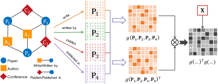
where represents a graph signal vector and we treat it as a column of the node features . As illustrated in Figure 1, our PSHGCN approximated a positive semidefinite heterogeneous graph convolution by the multiplication of . In practice, we employ two Multi-layer Perceptrons (MLPs) for feature extraction and downstream learning tasks, with one preceding and another following the convolution operator. More precisely, the PSHGCN model can be formulated as
where and denote MLPs. Interestingly, despite PSHGCN not being as powerful as the full Sum of Squares form, this simple approach demonstrates state-of-the-art (SOTA) performance in node classification tasks on heterogeneous graphs, as showcased in Section 6.
4 Analysis of PSHGCN
In this section, we delve into the underlying rationale of PSHGCN, with a particular emphasis on graph optimization. We will establish that PSHGCN represents the essential structure of any valid heterogeneous convolution. Additionally, we will analyze the complexity and scalability of our PSHGCN approach.
4.1 Generalized Heterogeneous Graph Optimization Framework
The utilization of graph optimization in designing GNNs for homogeneous graphs has been extensively explored and has led to remarkable performance achievements [37, 30, 7, 38]. However, there have been limited efforts to extend the graph optimization framework to heterogeneous graphs. Given an -dimensional graph signal , we consider a generalized heterogeneous graph optimization problem
| (7) |
where is a trade-off parameter, denotes the resulting representation of the input signal , and is an energy function determining the rate of propagation [18]. Generally, takes the shift operators as inputs and produces a real matrix. We can express certain existing heterogeneous graph optimization objectives with the generalized graph optimization framework. For example, by setting subject to and , the optimization function (7) corresponds to the objective used in EMRGNN [26].
We establish a "minimum requirement" for the energy function , demanding that its output matrix must be positive semidefinite. Failure to meet this requirement renders the optimization function non-convex. Conversely, if the output of is positive semidefinite, problem (7) admits a closed-form solution. We compute the derivative of with respect to and we have
| (8) |
Set the derivative to zero and we obtain the optimal solution
| (9) |
We can observe that is the heterogeneous graph convolution, and we denote it as , i.e., .
4.2 Positive Semidefinite Constraint on Graph Convolution
Given an arbitrary energy function whose output is positive semidefinite, we now consider how the corresponding heterogeneous graph convolution should look like. Specifically, we present the following lemma.
Lemma 4.1.
Consider an arbitrary energy function whose output is a real positive semidefinite matrix and , then the matrix is also a real positive semidefinite matrix.
The derivation of this Lemma is shown in the supplementary materials. Lemma 4.1 demonstrates that, within our generalized heterogeneous graph optimization framework, the heterogeneous graph convolution must be positive semidefinite. This observation motivates our PSHGCN, whose learned convolution is ensured to be positive semidefinite. Specifically, according to Taylor’s theorem for multivariate function [14], we approximate the heterogeneous graph convolution with a multivariate polynomial, denoted as . Theorem 3.1 implies that we should employ the Sum of Squares form to obtain a positive semidefinite polynomial for the heterogeneous graph convolution .
4.3 Complexity and Scalability
In the Equation (6), we assume the dimension of ’s output is and represents a -order monomial noncommutative polynomial similar to Equation (3). Theoretically, the polynomial has terms. However, in practice, many terms in are zero matrices due to various types of nodes have no direct connections from each other in heterogeneous graphs, such as authors and conferences in DBLP. Consequently, we can eliminate these terms. Let represent the count of non-zero terms with order in polynomial , and let represent the maximum number of edges in . We can get the time complexity of PSHGCN as . This complexity is comparable to that of many meta-path based HGNNs. The constant can be interpreted as the number of selected meta-paths, and can be seen as the maximum length of meta-paths.
Similar to many popular spectral-based GNNs, our PSHGCN can be extended to large-scale graphs by decoupling the feature transformation and propagation processes. In particular, we first calculate and store for in the preprocessing, where is defined in Equation (3). Then we have the following propagation process:
| (10) |
where denotes the multiplication between the coefficients in and when we expand their multiplication, such as . The pre-computed allows us to train PSHGCN in a mini-batch manner. In our experiments, we assess the scalability of PSHGCN on ogbn-mag and find that PSHGCN achieves a new SOTA result.
5 Related Work
Graph Neural Networks. Graph neural networks (GNNs) are machine-learning techniques designed specifically for graph data. These methods aim to find a low-dimensional vector representation for each node, enabling efficient processing for various network mining tasks. GNNs can be broadly classified into two categories: spatial-based and spectral-based approaches [27].
Spatial-based GNNs employ direct propagation and aggregation of information within the spatial domain. From this viewpoint, GCN [12] can be interpreted as aggregating one-hop neighbor information in the graph. GAT [22] leverages attention mechanisms to learn aggregation weights.
Spectral-based GNNs utilize spectral graph convolutions/filters designed in the spectral domain. ChebNet [4] employs Chebyshev polynomials to approximate filters. GCN [12] simplifies the Chebyshev filter by utilizing a first-order approximation. APPNP [13] uses Personalized PageRank (PPR) to determine the filter weights. GPR-GNN [3] learns polynomial filters by employing gradient descent on the polynomial weights. BernNet [7] utilizes the Bernstein basis for approximating graph convolutions, enabling the learning of arbitrary graph filters. JacobiConv [25] and ChebNetII [8] use Jacobi polynomials and Chebyshev interpolation, respectively, to learn filters. These methods are designed for homogeneous graphs and may not perform optimally on heterogeneous graphs.
Heterogeneous Graph Neural Networks. Heterogeneous graphs encompass various types of nodes and edges, offering rich semantic information alongside structural details. Heterogeneous graph neural networks (HGNNs) are explicitly developed to address the challenges posed by heterogeneity. HGNNs can be broadly categorized into meta-path-based and meta-path-free HGNNs [29].
Meta-path-based HGNNs propagate and aggregate neighbor features using selected meta-paths. HAN [23] uses a hierarchical attention mechanism with multiple meta-paths for aggregating node features and semantic information. HetGNN [34] employs random walks to generate node neighbors and aggregates their features. MAGNN [5] encodes information from manually-selected meta-paths instead of just focusing on endpoints. SeHGNN [29] utilizes predetermined meta-paths for neighbor aggregations and applies a transformer-based approach for feature fusion.
Meta-path-free HGNNs propagate and aggregate messages from neighboring nodes in a manner similar to GNNs, without requiring a selected meta-path. RGCN [17] extends GCN [12] to heterogeneous graphs with edge type-specific graph convolutions. GTN [33] utilizes soft sub-graph selection and matrix multiplication to generate meta-path neighbor graphs. HGB [16] incorporates a multi-layer GAT network with attention based on node features and learnable edge-type embeddings. MHGCN [32] learns meta-paths through multi-layer convolution aggregation and employs GCN’s convolution for feature aggregation. EMRGNN [26] and HALO [1] propose optimization objectives tailored for heterogeneous graphs and design new HGNN architectures based on solving these optimization problems. All the HGNNs design their propagation modules within the spatial domain, which leads to a deficiency in theoretical explanation and controllability. This motivates the design of the proposed PSHGCN, which extends spectral-based GNNs to heterogeneous graphs, enabling the learning of spectral heterogeneous graph convolutions.
| Dataset | #Nodes |
|
#Edges |
|
Target | #Classes | ||||
| DBLP | 26,128 | 4 | 239,566 | 6 | author | 4 | ||||
| ACM | 10,942 | 4 | 547,872 | 8 | paper | 3 | ||||
| IMDB | 21,420 | 4 | 86,642 | 6 | movie | 5 | ||||
| AMiner | 55,783 | 3 | 153,676 | 4 | paper | 4 | ||||
| Ogbn-mag | 1,939,743 | 4 | 21,111,007 | 4 | paper | 349 |
6 Experiments
In this section, we conduct experiments to evaluate the performance of SHGCN against the state-of-the-art heterogeneous graph neural networks on a wide variety of open graph datasets.
Datasets and Experimental setup. We evaluate PSHGCN on five widely-used heterogeneous graphs for node classification tasks. The datasets include three academic citation heterogeneous graphs DBLP [16], ACM [16] and AMiner [24], a movie rating heterogeneous graph IMDB [16], and a large-scale academic citation heterogeneous graph ogbn-mag from OGB benchmark [10]. We list the details of the datasets in Table 2. All the experiments are carried out on a machine with an NVIDIA Tesla A100 GPU (80 GB memory), Intel Xeon CPU (2.30 GHz) with 64 cores, and 512 GB of RAM.
| DBLP | ACM | IMDB | AMiner | |||||
| Macro-F1 | Micro-F1 | Macro-F1 | Micro-F1 | Macro-F1 | Micro-F1 | Macro-F1 | Micro-F1 | |
| GCN | 90.84 | 91.47 | 92.17 | 92.12 | 57.88 | 64.82 | 75.63 | 85.77 |
| GAT | 93.83 | 93.39 | 92.26 | 92.19 | 58.94 | 64.86 | 75.23 | 85.56 |
| GPRGNN | 91.66 | 92.45 | 92.36 | 92.28 | 58.90 | 64.84 | 75.32 | 86.13 |
| ChebNetII | 92.05 | 92.97 | 92.45 | 92.33 | 58.07 | 64.79 | 75.59 | 85.82 |
| RGCN | 91.52 | 92.07 | 91.55 | 91.41 | 58.85 | 62.05 | 63.03 | 82.79 |
| HAN | 91.67 | 92.05 | 90.89 | 90.79 | 57.74 | 64.63 | 63.86 | 82.95 |
| GTN | 93.52 | 93.97 | 91.31 | 91.20 | 60.47 | 65.14 | 72.39 | 84.74 |
| MAGNN | 93.28 | 93.76 | 90.88 | 90.77 | 56.49 | 64.67 | 71.56 | 83.48 |
| EMRGNN | 92.19 | 92.57 | 92.93 | 93.85 | 61.87 | 65.86 | 73.74 | 85.46 |
| MHGCN | 93.56 | 94.03 | 92.12 | 91.97 | 62.85 | 66.57 | 73.56 | 85.18 |
| HGB | 94.01 | 94.46 | 93.42 | 93.35 | 63.53 | 67.36 | 75.43 | 86.52 |
| HALO | 92.37 | 92.84 | 93.05 | 92.96 | 71.63 | 73.81 | 74.91 | 87.25 |
| SeHGNN | 95.06 | 95.42 | 94.05 | 93.98 | 67.11 | 69.17 | 76.83 | 86.96 |
| PSHGCN | 95.21 | 95.53 | 94.35 | 94.27 | 72.33 | 74.46 | 77.26 | 88.21 |
6.1 Node Classification
Setting and baselines. For the node classification task, we first compare PSHGCN to four popular homogeneous GNNs, including GCN[12], GAT [22], GPRGNN [3] and ChebNetII [8], where GPRGNN and ChebNetII are two famous spectral-based GNNs. Additionally, we also compare PSHGCN to nine competitive HGNNs, including RGCN [17], HAN [23], GTN [33], MAGNN [5], EMRGNN [26], MHGCN [32], HGB [16], HALO [1] and SeHGNN [29]. To ensure a fair comparison, we adopt the experimental setup used in the HGB benchmark [16]. Specifically, we follow the standard split with the training/validation/test sets accounting for 24%/6%/70%. We use the existing baseline results provided by HGB [16]. For results that are not available, we use the officially released code and conduct a hyperparameter search based on the guidelines presented in their respective paper.
For PSHGCN, we use Equation (6) as the propagation process and set to normalized adjacency matrix . Since these datasets have diverse node types with varying dimensional features, we initially use feature projection to align them into the same data space, following a common practice in HGNNs [29, 16, 26]. We optimize the order from 1 to 5 in the polynomial . We use a uniform distribution to randomly initialize the weights in and optimize them using gradient descent, consistent with spectral-based GNNs [3, 7, 8]. More details of hyper-parameters and settings are listed in supplementary materials.
Results. We use the mean F1 scores with standard errors over five runs as the evaluation metric. Table 3 reports the results, and the best-performing two results are highlighted by boldface letters and underlining, respectively. We observe that the spectral-based GNNs, specially designed for homogeneous graphs, outperform certain HGNNs, indicating their promising effectiveness on heterogeneous graphs. Additionally, PSHGCN outperforms other methods on all datasets. The superiority of PSHGCN can be attributed to its capability of approximating various valid graph convolutions through learning the weights in and imposing the constraint of positive semidefiniteness on the learned convolution.
| Methods | Validation accuracy | Test accuracy |
| RGCN | 48.35 | 47.37 |
| HGT | 49.89 | 49.27 |
| NARS | 51.85 | 50.88 |
| SAGN | 52.25 | 51.17 |
| GAMLP | 53.23 | 51.63 |
| SeHGNN | 55.95 | 53.99 |
| PSHGCN | 56.16 | 54.57 |
| SAGN∗ | 55.91 | 54.40 |
| GAMLP∗ | 57.02 | 55.90 |
| SeHGNN∗ | 59.17 | 57.19 |
| PSHGCN∗ | 59.43 | 57.52 |
6.2 Scalability
To evaluate the scalability of PSHGCN, we conduct a node classification task on the large-scale heterogeneous graph ogbn-mag from the Open Graph Benchmark (OGB). We compare six baselines listed on the OGB leaderboard: RGCN [17], HGT [11], NARS [31], SAGN [20], GAMLP [36] and SeHGNN [29]. We use results on the leaderboard for these baselines. For PSHGCN, we use the process discussed in Section6.2, and more settings details are listed in supplementary materials.
Table 4 shows the mean accuracies with standard errors over five runs. We use the symbol ∗ to denote the usage of extra embeddings (e.g., ComplEx embedding) and multi-stage training, which are commonly used in the baselines. We observe that PSHGCN achieves a new SOTA result on ogbn-mag, highlighting its strong scalability and effectiveness.
6.3 Ablation Study
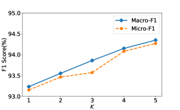
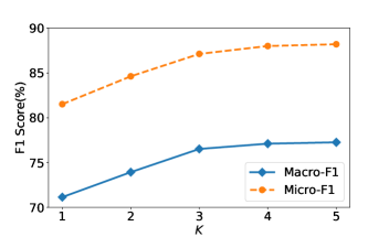
We investigate the impact of the order in the polynomial on the performance of PSGCN. Figure 2 displays the node classification F1 scores with respect to the order on ACM and AMiner (more results are listed in supplementary materials). We find that the performance of PSHGCN increases gradually with increasing , which is consistent with the theory of polynomial approximation in graph convolution. Notably, using excessively may result in too many weights, which can make the learning process challenging.
We explore the impact of the positive semidefinite constraint on PSHGCN by removing in Equation (6). For this variant, we search the optimal order from 2 to 10 and optimize the hyperparameters following the same procedure as PSHGCN. Table 5 presents the classification results of PSHGCN and the variant. We observe that PSHGCN outperforms this variant, particularly with lower standard errors. These findings highlight the effectiveness of our proposed positive semidefinite constraint in enhancing the capability of learning the convolution weights.
| DBLP | ACM | IMDB | AMiner | |||||
| Macro-F1 | Micro-F1 | Macro-F1 | Micro-F1 | Macro-F1 | Micro-F1 | Macro-F1 | Micro-F1 | |
| PSHGCN | 95.21 | 95.53 | 94.35 | 94.27 | 72.33 | 74.46 | 77.26 | 88.21 |
| VARIANT | 94.14 | 94.57 | 94.03 | 93.95 | 71.35 | 73.71 | 75.80 | 87.26 |
7 Discussion & Conclusion
This paper introduces PSHGCN, a novel heterogeneous convolutional network that extends spectral-based GNNs to heterogeneous graphs. Through the utilization of positive noncommutative polynomials, PSHGCN enables effective learning of diverse spectral heterogeneous graph convolutions. Experimental results demonstrate that PSHGCN achieves superior performance in node classification tasks compared to existing methods. Notably, PSHGCN is the first model that attempts to learn polynomial spectral graph convolutions on heterogeneous graphs, opening up various avenues for future exploration. For example, challenges remain when using PSHGCN to handle heterogeneous graphs with numerous node types and edge types, a predicament faced by most existing HGNNs. There are also problems regarding the definition of the Fourier transform on heterogeneous graphs and the utilization of other multivariable polynomial bases to learn the heterogeneous convolutions.
References
- [1] Hongjoon Ahn, Youngyi Yang, Quan Gan, David Wipf, and Taesup Moon. Descent steps of a relation-aware energy produce heterogeneous graph neural networks. In NeurIPS, 2022.
- [2] Lei Cai, Jundong Li, Jie Wang, and Shuiwang Ji. Line graph neural networks for link prediction. IEEE Transactions on Pattern Analysis and Machine Intelligence, 2021.
- [3] Eli Chien, Jianhao Peng, Pan Li, and Olgica Milenkovic. Adaptive universal generalized pagerank graph neural network. In ICLR, 2021.
- [4] Michaël Defferrard, Xavier Bresson, and Pierre Vandergheynst. Convolutional neural networks on graphs with fast localized spectral filtering. In NeurIPS, pages 3844–3852, 2016.
- [5] Xinyu Fu, Jiani Zhang, Ziqiao Meng, and Irwin King. Magnn: Metapath aggregated graph neural network for heterogeneous graph embedding. In TheWebConf, pages 2331–2341, 2020.
- [6] Zhongkai Hao, Chengqiang Lu, Zhenya Huang, Hao Wang, Zheyuan Hu, Qi Liu, Enhong Chen, and Cheekong Lee. Asgn: An active semi-supervised graph neural network for molecular property prediction. In KDD, pages 731–752, 2020.
- [7] Mingguo He, Zhewei Wei, Zengfeng Huang, and Hongteng Xu. Bernnet: Learning arbitrary graph spectral filters via bernstein approximation. In NeurIPS, 2021.
- [8] Mingguo He, Zhewei Wei, and Ji-Rong Wen. Convolutional neural networks on graphs with chebyshev approximation, revisited. In NeurIPS, 2022.
- [9] J William Helton. " positive" noncommutative polynomials are sums of squares. Annals of Mathematics, pages 675–694, 2002.
- [10] Weihua Hu, Matthias Fey, Marinka Zitnik, Yuxiao Dong, Hongyu Ren, Bowen Liu, Michele Catasta, and Jure Leskovec. Open graph benchmark: Datasets for machine learning on graphs. Advances in neural information processing systems, 33:22118–22133, 2020.
- [11] Ziniu Hu, Yuxiao Dong, Kuansan Wang, and Yizhou Sun. Heterogeneous graph transformer. In TheWebConf, pages 2704–2710, 2020.
- [12] Thomas N Kipf and Max Welling. Semi-supervised classification with graph convolutional networks. In ICLR, 2017.
- [13] Johannes Klicpera, Aleksandar Bojchevski, and Stephan Günnemann. Predict then propagate: Graph neural networks meet personalized pagerank. In ICLR, 2019.
- [14] Konrad Königsberger. Analysis 2. Springer-Verlag, 2013.
- [15] Qi Liu, Maximilian Nickel, and Douwe Kiela. Hyperbolic graph neural networks. Advances in Neural Information Processing Systems, 32, 2019.
- [16] Qingsong Lv, Ming Ding, Qiang Liu, Yuxiang Chen, Wenzheng Feng, Siming He, Chang Zhou, Jianguo Jiang, Yuxiao Dong, and Jie Tang. Are we really making much progress? revisiting, benchmarking and refining heterogeneous graph neural networks. In KDD, pages 1150–1160, 2021.
- [17] Michael Schlichtkrull, Thomas N Kipf, Peter Bloem, Rianne van den Berg, Ivan Titov, and Max Welling. Modeling relational data with graph convolutional networks. In European semantic web conference, pages 593–607. Springer, 2018.
- [18] Daniel Spielman. Spectral and algebraic graph theory. Yale lecture notes, draft of December, 4, 2019.
- [19] Ljubisa Stankovic, Danilo Mandic, Milos Dakovic, Milos Brajovic, Bruno Scalzo, and Tony Constantinides. Graph signal processing–part i: Graphs, graph spectra, and spectral clustering. arXiv preprint arXiv:1907.03467, 2019.
- [20] Chuxiong Sun, Hongming Gu, and Jie Hu. Scalable and adaptive graph neural networks with self-label-enhanced training. arXiv preprint arXiv:2104.09376, 2021.
- [21] Yizhou Sun and Jiawei Han. Mining heterogeneous information networks: principles and methodologies. Synthesis Lectures on Data Mining and Knowledge Discovery, 3(2):1–159, 2012.
- [22] Petar Veličković, Guillem Cucurull, Arantxa Casanova, Adriana Romero, Pietro Lio, and Yoshua Bengio. Graph attention networks. In ICLR, 2018.
- [23] Xiao Wang, Houye Ji, Chuan Shi, Bai Wang, Yanfang Ye, Peng Cui, and Philip S Yu. Heterogeneous graph attention network. In TheWebConf, pages 2022–2032, 2019.
- [24] Xiao Wang, Nian Liu, Hui Han, and Chuan Shi. Self-supervised heterogeneous graph neural network with co-contrastive learning. In KDD, pages 1726–1736, 2021.
- [25] Xiyuan Wang and Muhan Zhang. How powerful are spectral graph neural networks. In ICML, 2022.
- [26] Yuling Wang, Hao Xu, Yanhua Yu, Mengdi Zhang, Zhenhao Li, Yuji Yang, and Wei Wu. Ensemble multi-relational graph neural networks. In IJCAI, pages 2298–2304, 2022.
- [27] Zonghan Wu, Shirui Pan, Fengwen Chen, Guodong Long, Chengqi Zhang, and S Yu Philip. A comprehensive survey on graph neural networks. IEEE transactions on neural networks and learning systems, 2020.
- [28] Keyulu Xu, Weihua Hu, Jure Leskovec, and Stefanie Jegelka. How powerful are graph neural networks? In ICLR, 2018.
- [29] Xiaocheng Yang, Mingyu Yan, Shirui Pan, Xiaochun Ye, and Dongrui Fan. Simple and efficient heterogeneous graph neural network. In AAAI, 2022.
- [30] Yongyi Yang, Tang Liu, Yangkun Wang, Jinjing Zhou, Quan Gan, Zhewei Wei, Zheng Zhang, Zengfeng Huang, and David Wipf. Graph neural networks inspired by classical iterative algorithms. In ICML. PMLR, 2021.
- [31] Lingfan Yu, Jiajun Shen, Jinyang Li, and Adam Lerer. Scalable graph neural networks for heterogeneous graphs. arXiv preprint arXiv:2011.09679, 2020.
- [32] Pengyang Yu, Chaofan Fu, Yanwei Yu, Chao Huang, Zhongying Zhao, and Junyu Dong. Multiplex heterogeneous graph convolutional network. In KDD, pages 2377–2387, 2022.
- [33] Seongjun Yun, Minbyul Jeong, Raehyun Kim, Jaewoo Kang, and Hyunwoo J Kim. Graph transformer networks. Advances in neural information processing systems, 32, 2019.
- [34] Chuxu Zhang, Dongjin Song, Chao Huang, Ananthram Swami, and Nitesh V Chawla. Heterogeneous graph neural network. In KDD, pages 793–803, 2019.
- [35] Muhan Zhang and Yixin Chen. Link prediction based on graph neural networks. Advances in neural information processing systems, 31, 2018.
- [36] Wentao Zhang, Ziqi Yin, Zeang Sheng, Yang Li, Wen Ouyang, Xiaosen Li, Yangyu Tao, Zhi Yang, and Bin Cui. Graph attention multi-layer perceptron. In KDD, pages 4560–4570, 2022.
- [37] Dengyong Zhou, Olivier Bousquet, Thomas Lal, Jason Weston, and Bernhard Schölkopf. Learning with local and global consistency. Advances in neural information processing systems, 16, 2003.
- [38] Meiqi Zhu, Xiao Wang, Chuan Shi, Houye Ji, and Peng Cui. Interpreting and unifying graph neural networks with an optimization framework. In TheWebConf, pages 1215–1226, 2021.
- [39] Zhaocheng Zhu, Zuobai Zhang, Louis-Pascal Xhonneux, and Jian Tang. Neural bellman-ford networks: A general graph neural network framework for link prediction. Advances in Neural Information Processing Systems, 34:29476–29490, 2021.