Unsupervised Anomaly Detection in Medical Images Using Masked Diffusion Model

Abstract

It can be challenging to identify brain MRI anomalies using supervised deep-learning techniques due to anatomical heterogeneity and the requirement for pixel-level labeling. Unsupervised anomaly detection approaches provide an alternative solution by relying only on sample-level labels of healthy brains to generate a desired representation to identify abnormalities at the pixel level. Although, generative models are crucial for generating such anatomically consistent representations of healthy brains, accurately generating the intricate anatomy of the human brain remains a challenge. In this study, we present a method called the masked-denoising diffusion probabilistic model (mDDPM), which introduces masking-based regularization to reframe the generation task of diffusion models. Specifically, we introduce Masked Image Modeling (MIM) and Masked Frequency Modeling (MFM) in our self-supervised approach that enables models to learn visual representations from unlabeled data. To the best of our knowledge, this is the first attempt to apply MFM in denoising diffusion probabilistic models (DDPMs) for medical applications. We evaluate our approach on datasets containing tumors and numerous sclerosis lesions and exhibit the superior performance of our unsupervised method as compared to the existing fully/weakly supervised baselines. Project website: https://mddpm.github.io/.

1 Introduction

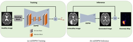
Figure 1: Schematic diagram of our framework. (a) During training, only healthy images are used, and no classifier guidance is required. The healthy image is passed through the Masking Block before feeding into the DDPM. The reconstruction loss is calculated between the original image and the image generated by the DDPM. Here, Masking Block plays the role of regularizer and eliminates the need for classifier guidance which is discussed in Section 2. Further, the schematic of the Masking Block is illustrated in Fig. 2. (b) During inference, DDPM considers the tumor in the unhealthy image as an augmented patch and eliminates it to generate a healthy image. The difference between the generated image and the given unhealthy image is then calculated to report the anomaly map. No masking mechanism is employed at inference.

Medical imaging (MI) systems play a crucial role in aiding radiologists in their diagnostic and decision-making processes. These systems provide medical imaging specialists with detailed visual information to detect abnormalities, make accurate diagnoses, plan treatments, and monitor patients. More recently, advanced machine learning techniques and image processing algorithms are being utilized to automate the medical diagnostic process. Among these techniques, deep learning models based on convolutional neural networks (CNNs) have exhibited significant achievements in accurately identifying anomalies in medical images [30, 12]. However, supervised CNN approaches have inherent limitations, including the requirement for extensive expert-annotated training data and the difficulty of learning from noisy or imbalanced data [11, 17, 16]. On the contrary, pixel-level annotations are not necessary for unsupervised anomaly detection (UAD) that uses only healthy examples for training.

In recent years, numerous architectures have been explored to investigate UAD for brain MRI anomaly detection. Autoencoders (AE) and variational autoencoders (VAE) have proven to be effective in training models and achieving efficient inference. However, their reconstructions often suffer from blurriness, limiting their effectiveness in UAD [3]. To address this limitation, researchers have focused on enhancing the understanding of image context by utilizing the spatial context through techniques such as spatial erasing [35] and leveraging 3D information [6, 4]. Additionally, vector-quantized VAEs [26], adversarial autoencoders [7], and encoder activation maps [31] have been proposed to improve the image restoration quality. Generative adversarial networks (GANs) have emerged as an alternative to AE-based architectures for the task of UAD [29]. However, the unstable training nature of GANs poses challenges, and GANs often suffer from mode collapse and a lack of anatomical coherence [3, 22].

Recently, denoising diffusion probabilistic models (DDPMs) [15] have shown promise for UAD in brain MRI [34, 5, 25]. In the context of DDPMs, the approach involves introducing noise to an input image and subsequently utilizing a trained model to eliminate the noise and estimate or reconstruct the original image [15]. Unlike most autoencoder-based methods, DDPMs retain spatial information in their hidden representations, which is crucial for the image generation process [27]. Recent works in medical imaging establish that they exhibit scalable and stable training properties and generate high-quality, sharp images with classifier guidance [33, 34, 28, 25, 26]. Further, [5, 24, 21] introduce patch-based DDPM (pDDPM) which offer better brain MRI reconstruction by incorporating global context information about individual brain structures and appearances while estimating individual patches.

Given the advantages observed when applying Mask Image Modeling (MIM) in conjunction with VAE frameworks [32, 13, 14], such as enhanced generalization capabilities and the acquisition of a comprehensive understanding of the structural characteristics of images, we introduce the first investigation into leveraging Masked Image Modeling (MIM) and Masked Frequency Modeling (MFM) within DDPMs. In our proposed framework, masked DDPM (mDDPM), the need for the classifier guidance is eliminated. The masking mechanism proposed in our framework serves as a unique regularizer that enables the incorporation of global information while preserving fine-grained local features. This regularization technique imposes a constraint on DDPM, ensuring the generation of a healthy image during inference, regardless of the input image characteristics. In this study, we focus on exploring three specific variants of masking-based regularization: (i) image patch-masking (IPM), (ii) frequency patch-masking (FPM), and (iii) frequency patch-masking CutMix (FPM-CM). In the IPM approach, random pixel-level masks are applied to patches extracted from the original image before subjecting them to the diffusion process in DDPMs. The unmasked version of the same image is used as the reference for comparison. However, in the FPM approach, the image is first transformed into the frequency domain using the Fast Fourier Transform. Subsequently, patch-level masking is performed in the frequency domain as shown in Figure 2a. The inverse Fourier Transform is then applied to obtain the reconstructed image, which is utilized to calculate the reconstruction loss. In FPM-CM, random patches are sampled from the augmented image generated through FPM and subsequently inserted at corresponding positions within the original clean image as shown in Figure 2b. To evaluate the performance of our method, we use two publicly available datasets: BraTS21 [2], and MSLUB [20], and demonstrate a significant improvement (p $<$ 0.05) in tumor segmentation performance.

2 Method

Given the potential occurrence of anomalies in any region of the brain during testing, we introduce data augmentation techniques that involve the insertion of random augmented patches into the healthy input image, $\bm{z}\in\mathbb{R}^{C,W,H}$ with $C$ channels, width $W$ and height $H$, prior to the application of DDPM noise addition and removal. This approach allows us to generate a healthy image based on an unhealthy image during inference, facilitating the calculation of the anomaly map. The illustration of our approach can be seen in Figure 1. We will be further discussing our unsupervised mDDPM approach and proposed masking strategies in this section.

2.1 Fourier Transform

We first briefly introduce the Discrete Fourier Transform (DFT) as it plays a crucial role in our mDDPM approach. Given a 2D signal $\bm{z}\in\mathbb{R}^{W\times H}$, the corresponding 2D-DFT, a widely used signal analysis technique, can be defined as follows:

$$\small f(x,y)=\sum_{h=0}^{H-1}\sum_{w=0}^{W-1}{z}{(h,w)}e^{-j2\pi\left(\frac{xh}{H}+\frac{yw}{W}\right)},$$ (1)

$z{(h,w)}$ denotes the signal located at position $(h,w)$ in $\bm{z}$, while $x$ and $y$ serve as indices representing the horizontal and vertical spatial frequencies in the Fourier spectrum. The inverse 2D DFT (2D-IDFT) is defined as:

$$\small F(h,w)=\frac{1}{HW}\sum_{x=0}^{H-1}\sum_{y=0}^{W-1}f(x,y)e^{j2\pi\left(\frac{xh}{H}+\frac{yw}{W}\right)},$$ (2)

Both the DFT and IDFT can be efficiently computed using the Fast Fourier Transform (FFT) algorithm, as in [23].

In the context of medical images with various modalities, the Fourier Transform is applied independently to each channel. Additionally, previous works such as [32, 8, 19] have demonstrated that the high-frequency part of the Fourier spectrum contains detailed structural texture information, while the low-frequency part contains global information.

2.2 DDPMs

In DDPMs, the forward process involves gradually introducing noise to the input image $\bm{z}_{0}$ according to a predefined schedule $\beta_{1},...,\beta_{T}$. The noise is sampled from a Gaussian distribution $\mathcal{N}(\textbf{0},\textbf{I})$, and at each time step $t$, the noisy image $\bm{z}_{t}$ is generated as follows:

$$\bm{z}_{t}\sim q(\bm{z}_{t}|\bm{z}_{0})=\mathcal{N}(\sqrt{\bar{\alpha}_{t}}\bm{z}_{0},(1-\bar{\alpha}_{t})\textbf{I}),$$ (3)

where $\bar{\alpha}_{t}=\prod\nolimits_{s=0}^{t}(1-\beta_{t})$ and $t$ is sampled from a uniform distribution. For $t=T$, the image becomes pure Gaussian noise $\bm{z}_{t}=\bm{\epsilon}\sim\mathcal{N}(\textbf{0},\textbf{I})$, while for $t=0$, $\bm{z}_{t}$ remains $\bm{x}_{0}$.

In the denoising process, the objective is to reverse the forward process and reconstruct the original image $\bm{z}_{0}$. The reconstruction is achieved by sampling $\bm{z}_{0}$ from the joint distribution:

$$\bm{z}_{0}\sim p_{\theta}(\bm{z_{t}})\prod\nolimits^{T}_{t=1}p_{\theta}(\bm{z}_{t-1}|\bm{z}_{t}),$$ (4)

where $p_{\theta}(\bm{z}_{t-1}|\bm{z}_{t})$ is modeled as a Gaussian distribution $\mathcal{N}(\bm{\mu}_{\theta}(\bm{z}_{t},t),\bm{\Sigma}_{\theta}(\bm{z}_{t},t))$. The parameters $\bm{\mu}_{\theta}$ and $\bm{\Sigma}_{\theta}$ are estimated by a neural network, and we use a U-Net architecture for this purpose. The covariance $\bm{\Sigma}_{\theta}(\bm{z}_{t},t)$ is fixed as $\frac{1-\alpha_{t-1}}{1-\alpha_{t}}\beta_{t}\textbf{I}$, following the approach in [15]. In this work, we simplify the loss derivation by directly estimating the reconstruction $\bm{z}^{{}^{\prime}}_{0}\sim p_{\theta}(\bm{z}_{0}|\bm{z}_{t},t)$ as in  [5] and using the mean absolute error ($l1$-error) as the loss function:

$$\mathcal{L}_{rec}=|\bm{z}_{0}-\bm{z}^{{}^{\prime}}_{0}|,$$ (5)

Instead of performing step-wise denoising for all time steps starting from $t=T$, as commonly done for sampling images with DDPMs, we directly estimate $\bm{z}^{{}^{\prime}}_{0}$ at a fixed time step $t_{fix}$.

2.3 Masked DDPMs

As stated above, we model mDDPM by introducing a Masking block before DDPM stage as shown in Fig. 1 that can be incorporated in three different forms during training, namely IPM, FPM, and FPM-CM.

2.3.1 Image Patch-Masking (IPM)

In the IPM approach, random masks are applied at the pixel level to patches extracted from the original image. The masked image is then subjected to the diffusion process in DDPMs. In contrast, the unmasked version of the same image is used as a reference for comparison during training. For reference, the output of the IPM block can be observed in Fig. 2b.

During training, we sample $N$ patch regions, $[p_{1},p_{2},...,p_{N}]$ at random positions such that $\Sigma_{n=0}^{N}{A_{n}}<A_{z}$, where ${A_{n}}$ is the area of patch $p_{n}$, and ${A_{z}}$ is the area of image, $\bm{z}$ in pixel space. Let $\bm{M^{I}_{p}}\in\mathbb{R}^{C,H,W}$ be a binary mask in the pixel domain that indicates which pixels overlap with the patches $[p_{1},p_{2},...,p_{N}]$. Specifically, the pixels within each $\bm{p_{n}}$ are assigned a value of zero, while the pixels outside of $\bm{p_{n}}$ are assigned a value of one. We obtain $\bm{z_{M}}$, by combining the original image $\bm{z_{0}}$ with the masked region using element-wise multiplication:

$$\bm{z^{I}_{M}}=\bm{z}_{0}\odot\bm{M^{I}_{p}},$$ (6)

Here, $\odot$ represents the Hadamard product. $\bm{z_{M}}$ is then fed to DDPM forward process.

In the backward process, the denoised image, denoted as $\bm{\tilde{z}}_{0}$, is generated by the network as an estimate of the original image $\bm{z}_{0}$. As we calculate the absolute difference between the original image $\bm{z}_{0}$ and the denoised image $\bm{\tilde{z}_{0}}$ during training, the objective function $\mathcal{L}_{M}=\mathcal{L}_{rec}$, where $\mathcal{L}_{rec}$ is defined in Eq. 5.

By applying random pixel-level masks to the patches, the IPM approach introduces a form of regularization that encourages the DDPMs to generate images that closely resemble the unmasked reference image.

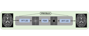
(a) Block diagram of FPM. Here, Fast Fourier Transform is performed on each slice, and then masking is performed on the frequency spectrum. The Inverse Fourier Transform of this masked spectrum outputs an augmented image of the input image.

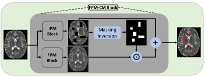
(b) Block diagram of FPM-CM. Here, random patches are chosen from the augmented image obtained after FPM. These selected patches are then inserted at the corresponding positions in the original clean image to generated an augmented image.

Figure 2: Proposed data augmentation techniques which are implemented in the Masking Block of the Fig. 1.

2.3.2 Frequency Patch-Masking (FPM)

The proposed FPM mechanism has been illustrated in Fig. 2a. FPM block mainly consists of three blocks, FFT-2D, frequency spectrum masking (FSM), and IFFT-2D. Here, the image undergoes a series of transformations in the frequency domain using the Fast Fourier Transform (FFT). The Fast Fourier Transform allows us to analyze the image in terms of different frequencies present within it. After the image is transformed into the frequency domain, patch-level masking is performed using a binary mask $\bm{M^{F}_{p}}$ similar to the one used in IPM. This means that specific regions or patches within the frequency representation of the image are masked out. Masking in the frequency domain allows for selective modification of certain frequency components of the image while leaving others intact. Here, we don’t specify the high-frequency or low-frequency masking, rather MFM is performed randomly. Once the patch-level masking is complete, the inverse Fourier Transform is applied to the modified frequency representation. This transforms the image back from the frequency domain to the spatial domain, reconstructing the modified image. The FPM block is mathematically formulated as,

$$\bm{z^{F}_{M}}=IDFT(\bm{M^{F}_{p}}\odot DFT(\bm{z_{0}})),$$ (7)

The reconstructed image is subsequently inputted into DDPM, utilizing the identical objective function as described earlier in Eq. 5.

2.3.3 Frequency Patch-Masking CutMix (FPM-CM)

FPM-CM extends the application of FPM to apply patched augmentation in the original image as shown in Fig. 2b. In FPM-CutMix, the image is first passed through an FPM augmentation stage, and then patches are sampled from this augmented image. These patches are essentially small rectangular regions with varying sizes that capture specific features or information from the augmented image. After sampling the patches, they are inserted into the original clean image at corresponding positions. This means that the patches are placed in the same spatial locations within the original image as they were in the augmented image. By inserting the patches at corresponding positions, the intention is to transfer the modified features from the augmented image to the original clean image. It can be observed that these augmented patches behave as anomalies during training as the key idea is to use DDPM to generate the clean un-augmented image. Therefore such augmentation serves the purpose of unsupervised anomaly training. Assuming that we have obtained $\bm{z^{I}_{M}}$, and $\bm{z^{F}_{M}}$ from IPM and FPM block respectively, FPM-CM can be mathematically written as,

$$\bm{z^{FC}_{M}}=\bm{z^{I}_{M}}+(\bm{z^{F}_{M}}\odot\neg\bm{M^{I}_{p}}),$$ (8)

Here, $\neg$ indicates binary inversion, and $\bm{z^{FC}_{M}}$ is the FPM-CM block output. We feed in DDPM with $\bm{z^{FC}_{M}}$ using the same objective function as used by other approaches mentioned above and stated in Eq. 5.

3 Experimental Evaluation

3.1 Implementation Details

For our experiments, we utilize the publicly available IXI dataset for training [1]. The IXI dataset comprises 560 pairs of T1 and T2-weighted brain MRI scans. To ensure robust evaluation, the IXI dataset is partitioned into eight folds, comprising 400/160 training/validation samples. To evaluate our approach, we employ two publicly available datasets: the Multimodal Brain Tumor Segmentation Challenge 2021 (BraTS21) dataset [2] and the multiple sclerosis dataset from the University Hospital of Ljubljana (MSLUB) [20]. The BraTS21 dataset includes 1251 brain MRI scans with four different weightings (T1, T1-CE, T2, FLAIR). Following [5], it was divided into a validation set of 100 samples and a test set of 1151 samples, both containing unhealthy scans. The MSLUB dataset consists of brain MRI scans from 30 multiple sclerosis (MS) patients, with each patient having T1, T2, and FLAIR-weighted scans. This dataset was split into a validation set of 10 samples and a test set of 20 samples as in  [5], all representing unhealthy scans. Thus, our training, validation, and testing data consist of 400, 270, and 1171 samples respectively. In all our experimental setups, we exclusively employ T2-weighted images extracted from the respective dataset and perform the pre-processing such as affine transformation, skull stripping, and downsampling as in  [5]. With the specifically designed pre-processing techniques, we filtered out the regions belonging to the foreground area so that Masking Block can only be applied to the foreground pixel patches.

We assess the performance of our proposed method, mDDPM, in comparison to various established baselines for UAD in brain MRI. These baselines include: (i) VAE [3], (ii) Sequential VAE (SVAE) [4], (iii) denoising AE (DAE) [18], the GAN-based (iv) f-AnoGAN [29], (v) DDPM [34], and (iv) patched DDPM (pDDPM), which feeds patched input to the DDPM. We evaluate all baseline methods via in-house training using their default parameters. For VAE, SVAE, and f-AnoGAN, we set the value of the hyperparameter according to [5]. For DDPM, pDDPM, and mDDPM, we employ structured simplex noise instead of Gaussian noise as it better captures the natural frequency distribution of MRI images [34]. We follow [5] for all other training and inference settings. By default, the models undergo training for 1600 epochs. During the training phase, the volumes are processed in a slice-wise fashion, where slices are uniformly sampled with replacement. However, during the testing phase, all slices are iterated over to reconstruct the entire volume. Further, we conducted all our experiments with a masking ratio randomly varying between 10%-90% of the whole foreground region.

3.2 Inference Criteria

During the training phase, all models are trained to minimize the $l1$ error between the healthy input image and its corresponding reconstruction. At the test stage, we utilize the reconstruction error as a pixel-wise anomaly score denoted as $\bm{\Lambda}_{S}=|\bm{z}_{0}-\bm{z}^{{}^{\prime}}_{0}|$, where higher values correspond to larger reconstruction errors.

To enhance the quality of the anomaly maps, we employ commonly used post-processing techniques [3, 35]. Prior to binarizing $\bm{\Lambda}_{S}$, we apply a median filter with a kernel size of $K_{M}=5$ to smooth the anomaly scores and perform brain mask erosion for three iterations. After binarization and calculating threshold as in  [5], we iteratively calculate DICE scores [10] for different thresholds and select the threshold that yields the highest average DICE score on the selected test set. Additionally, we record the average Area Under the Precision-Recall Curve (AUPRC) [9] on the test set.

Table 1: Comparison of the models under consideration, with the best outcomes denoted in bold using DICE and AUPRC as evaluation metrics.

Model	BraTS21		MSLUB
	DICE [%]	AUPRC [%]	DICE [%]	AUPRC [%]
VAE [3]	30.57$\pm$1.67	28.47$\pm$1.38	6.63$\pm$0.12	5.01$\pm$0.54
SVAE [4]	33.86$\pm$0.19	33.53$\pm$0.23	5.71$\pm$0.48	5.05$\pm$0.11
DAE [18]	36.85$\pm$1.62	45.19$\pm$1.35	3.67$\pm$0.82	5.24$\pm$0.53
f-AnoGAN [29]	24.44$\pm$2.28	22.52$\pm$2.37	4.29$\pm$1.02	4.09$\pm$0.79
DDPM [34]	40.82$\pm$1.34	49.82$\pm$1.13	8.52$\pm$1.42	8.44$\pm$1.54
pDDPM [5] + fixed sampling + $\mathcal{L}_{p}$	49.12$\pm$1.27	53.98$\pm$2.16	9.04$\pm$0.66	9.23$\pm$0.83
mDDPM (IPM)	52.16$\pm$1.64	58.12$\pm$1.56	10.39$\pm$0.88	10.58$\pm$0.92
mDDPM (FPM)	50.91$\pm$1.28	56.27$\pm$1.44	9.31$\pm$0.46	9.51$\pm$0.52
mDDPM (FPM-CM)	53.02$\pm$1.34	59.04$\pm$1.26	10.71$\pm$0.62	10.59$\pm$0.57

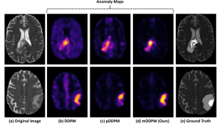
Figure 3: In the comparison of the qualitative results between mDDPM (FPM-CM) and the baselines, we present the anomaly map comparisons for two samples. In the first sample, mDDPM demonstrates a more precise detection of the anomaly, exhibiting a final anomaly map without foreground noise. Similarly, in the second sample, mDDPM performs closest to the ground truth in terms of anomaly detection as shown in the results of the second row where we only included results for the FPM-CM variant of our method.

3.3 Results

The comparison of our proposed mDDPM with the baseline method is presented in Table 1. It can be observed that our mDDPM outperforms all baseline approaches on both datasets in terms of DICE [10] and AUPRC [9]. In terms of qualitative evaluation, we observe smaller reconstruction errors from mDDPM compared to patched DDPM [5] for healthy brain anatomy, as shown in Fig. 3. It can be observed that, mDDPM (FPM-CM) showcases a higher level of precision in detecting the anomaly, resulting in an anomaly map that is free from foreground noise.

4 Conclusion

This study introduces an approach for reconstructing the healthy brain anatomy using masked DDPM, which incorporates image-mask and frequency-mask regularization. Our method, known as mDDPM, surpasses established baselines, even with unsupervised training. However, a limitation of the proposed approach is the increased inference time associated with the diffusion architecture. To address this, future research could concentrate on enhancing the efficiency of the diffusion denoising process by leveraging spatial context more effectively. Further, we intend to explore the Masked Diffusion Transformer architecture in our future studies where we can incorporate a latent modeling scheme using masks to specifically improve the contextual relationship learning capabilities of DDPMs for object semantic parts within an image.

References

- [1] https://brain-development.org/ixi-dataset/
- [2] Baid, U., Ghodasara, S., Mohan, S., Bilello, M., Calabrese, E., Colak, E., Farahani, K., Kalpathy-Cramer, J., Kitamura, F.C., Pati, S., et al.: The rsna-asnr-miccai brats 2021 benchmark on brain tumor segmentation and radiogenomic classification. arXiv preprint arXiv:2107.02314 (2021)
- [3] Baur, C., Denner, S., Wiestler, B., Navab, N., Albarqouni, S.: Autoencoders for unsupervised anomaly segmentation in brain mr images: a comparative study. Medical Image Analysis p. 101952 (2021)
- [4] Behrendt, F., Bengs, M., Bhattacharya, D., Krüger, J., Opfer, R., Schlaefer, A.: Capturing inter-slice dependencies of 3d brain mri-scans for unsupervised anomaly detection. In: Medical Imaging with Deep Learning (2022)
- [5] Behrendt, F., Bhattacharya, D., Krüger, J., Opfer, R., Schlaefer, A.: Patched diffusion models for unsupervised anomaly detection in brain mri. arXiv preprint arXiv:2303.03758 (2023)
- [6] Bengs, M., Behrendt, F., Krüger, J., Opfer, R., Schlaefer, A.: Three-dimensional deep learning with spatial erasing for unsupervised anomaly segmentation in brain mri. International journal of computer assisted radiology and surgery 16(9), 1413–1423 (2021)
- [7] Chen, X., Konukoglu, E.: Unsupervised Detection of Lesions in Brain MRI using Constrained Adversarial Auto-encoders. In: International Conference on Medical Imaging with Deep Learning (MIDL). Proceedings of Machine Learning Research, PMLR (2018)
- [8] Chen, Y., Fan, H., Xu, B., Yan, Z., Kalantidis, Y., Rohrbach, M., Yan, S., Feng, J.: Drop an octave: Reducing spatial redundancy in convolutional neural networks with octave convolution. In: Proceedings of the IEEE/CVF international conference on computer vision. pp. 3435–3444 (2019)
- [9] Davis, J., Goadrich, M.: The relationship between precision-recall and roc curves. In: Proceedings of the 23rd international conference on Machine learning. pp. 233–240 (2006)
- [10] Dice, L.R.: Measures of the amount of ecologic association between species. Ecology 26(3), 297–302 (1945)
- [11] Ellis, R.J., Sander, R.M., Limon, A.: Twelve key challenges in medical machine learning and solutions. Intelligence-Based Medicine 6, 100068 (2022)
- [12] Fernando, T., Gammulle, H., Denman, S., Sridharan, S., Fookes, C.: Deep learning for medical anomaly detection – a survey. ACM Comput. Surv. 54(7) (jul 2021). https://doi.org/10.1145/3464423, https://doi.org/10.1145/3464423
- [13] Gao, P., Ma, T., Li, H., Lin, Z., Dai, J., Qiao, Y.: Convmae: Masked convolution meets masked autoencoders (2022)
- [14] He, K., Chen, X., Xie, S., Li, Y., Dollár, P., Girshick, R.: Masked autoencoders are scalable vision learners (2021)
- [15] Ho, J., Jain, A., Abbeel, P.: Denoising diffusion probabilistic models. Advances in Neural Information Processing Systems 33, 6840–6851 (2020)
- [16] Johnson, J.M., Khoshgoftaar, T.M.: Survey on deep learning with class imbalance. Journal of Big Data 6(1), 1–54 (2019)
- [17] Karimi, D., Dou, H., Warfield, S.K., Gholipour, A.: Deep learning with noisy labels: Exploring techniques and remedies in medical image analysis. Medical Image Analysis 65, 101759 (2020)
- [18] Kascenas, A., Pugeault, N., O’Neil, A.Q.: Denoising autoencoders for unsupervised anomaly detection in brain mri. In: International Conference on Medical Imaging with Deep Learning (MIDL). Proceedings of Machine Learning Research, PMLR (2022)
- [19] Kauffmann, L., Ramanoël, S., Peyrin, C.: The neural bases of spatial frequency processing during scene perception. Frontiers in integrative neuroscience 8, 37 (2014)
- [20] Lesjak, Ž., Galimzianova, A., Koren, A., Lukin, M., Pernuš, F., Likar, B., Špiclin, Ž.: A novel public mr image dataset of multiple sclerosis patients with lesion segmentations based on multi-rater consensus. Neuroinformatics 16(1), 51–63 (2018)
- [21] Lugmayr, A., Danelljan, M., Romero, A., Yu, F., Timofte, R., Van Gool, L.: Repaint: Inpainting using denoising diffusion probabilistic models. In: Proceedings of the IEEE/CVF Conference on Computer Vision and Pattern Recognition. pp. 11461–11471 (2022)
- [22] Nguyen, B., Feldman, A., Bethapudi, S., Jennings, A., Willcocks, C.G.: Unsupervised region-based anomaly detection in brain mri with adversarial image inpainting. In: 2021 IEEE 18th international symposium on biomedical imaging (ISBI). pp. 1127–1131. IEEE (2021)
- [23] Nussbaumer, H.J., Nussbaumer, H.J.: The fast Fourier transform. Springer (1981)
- [24] Özdenizci, O., Legenstein, R.: Restoring vision in adverse weather conditions with patch-based denoising diffusion models. IEEE Transactions on Pattern Analysis and Machine Intelligence (2023)
- [25] Pinaya, W.H., Graham, M.S., Gray, R., Da Costa, P.F., Tudosiu, P.D., Wright, P., Mah, Y.H., MacKinnon, A.D., Teo, J.T., Jager, R., et al.: Fast unsupervised brain anomaly detection and segmentation with diffusion models. arXiv preprint arXiv:2206.03461 (2022)
- [26] Pinaya, W.H., Tudosiu, P.D., Gray, R., Rees, G., Nachev, P., Ourselin, S., Cardoso, M.J.: Unsupervised brain imaging 3d anomaly detection and segmentation with transformers. Medical Image Analysis 79, 102475 (2022)
- [27] Rombach, R., Blattmann, A., Lorenz, D., Esser, P., Ommer, B.: High-resolution image synthesis with latent diffusion models. In: Proceedings of the IEEE/CVF Conference on Computer Vision and Pattern Recognition. pp. 10684–10695 (2022)
- [28] Sanchez, P., Kascenas, A., Liu, X., O’Neil, A.Q., Tsaftaris, S.A.: What is healthy? generative counterfactual diffusion for lesion localization. In: MICCAI Workshop on Deep Generative Models. pp. 34–44. Springer (2022)
- [29] Schlegl, T., Seeböck, P., Waldstein, S.M., Langs, G., Schmidt-Erfurth, U.: f-AnoGAN: Fast unsupervised anomaly detection with generative adversarial networks. Medical image analysis 54, 30–44 (2019)
- [30] Shen, D., Wu, G., Suk, H.I.: Deep learning in medical image analysis. Annual review of biomedical engineering 19, 221 (2017)
- [31] Silva-Rodríguez, J., Naranjo, V., Dolz, J.: Constrained unsupervised anomaly segmentation. Medical Image Analysis 80, 102526 (2022)
- [32] Wang, W., Wang, J., Chen, C., Jiao, J., Sun, L., Cai, Y., Song, S., Li, J.: Fremae: Fourier transform meets masked autoencoders for medical image segmentation (2023)
- [33] Wolleb, J., Bieder, F., Sandkühler, R., Cattin, P.C.: Diffusion models for medical anomaly detection. arXiv preprint arXiv:2203.04306 (2022)
- [34] Wyatt, J., Leach, A., Schmon, S.M., Willcocks, C.G.: Anoddpm: Anomaly detection with denoising diffusion probabilistic models using simplex noise. In: Proceedings of the IEEE/CVF Conference on Computer Vision and Pattern Recognition. pp. 650–656 (2022)
- [35] Zimmerer, D., Kohl, S., Petersen, J., Isensee, F., Maier-Hein, K.: Context-encoding variational autoencoder for unsupervised anomaly detection. In: International Conference on Medical Imaging with Deep Learning–Extended Abstract Track (2019)