![[Uncaptioned image]](/html/2305.19858/assets/x1.png)
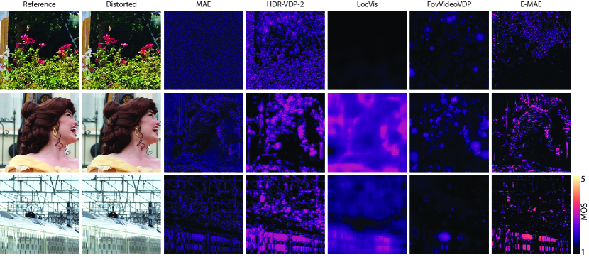
We introduce self-supervised visual masking that enhances image quality prediction for existing quality metrics such as MAE, SSIM, FLIP, and VGG. Our work is inspired by the well-known characteristic of the Human Visual System (HVS), visual masking, which results in locally varying sensitivity to image artifact visibility that reduces with increasing contrast magnitude of the original image pattern. We found that the learned masking clearly outperforms its traditional hand-crafted versions and better adapts to specific distortion patterns. In the first two rows, we show the reference and distorted images, while the third and fourth rows show the error maps as predicted by the original metrics and their enhanced versions using our masking approach. As can be seen, our mask-enhanced metrics better predict the local distortion visibility by the human observer. For a more intuitive comparison, we scale each error map to fit within the mean opinion scores (MOS) range (please refer to Sec. 4.2 for more details). In this color scale, darker indicates less visible distortion.
Enhancing image quality prediction with self-supervised visual masking
Abstract
Full-reference image quality metrics (FR-IQMs) aim to measure the visual differences between a pair of reference and distorted images, with the goal of accurately predicting human judgments. However, existing FR-IQMs, including traditional ones like PSNR and SSIM and even perceptual ones such as HDR-VDP, LPIPS, and DISTS, still fall short in capturing the complexities and nuances of human perception. In this work, rather than devising a novel IQM model, we seek to improve upon the perceptual quality of existing FR-IQM methods. We achieve this by considering visual masking, an important characteristic of the human visual system that changes its sensitivity to distortions as a function of local image content. Specifically, for a given FR-IQM metric, we propose to predict a visual masking model that modulates reference and distorted images in a way that penalizes the visual errors based on their visibility. Since the ground truth visual masks are difficult to obtain, we demonstrate how they can be derived in a self-supervised manner solely based on mean opinion scores (MOS) collected from an FR-IQM dataset. Our approach results in enhanced FR-IQM metrics that are more in line with human prediction both visually and quantitatively. Plase refer to https://enhancediqm.mpi-inf.mpg.de/ for supplementary materials.

1 Introduction
Full-Reference Image Quality Metrics (FR-IQMs), which take as an input a pair of reference and distorted images, play a crucial role in a wide range of applications in digital image processing, such as image compression and transmission, as well as in evaluating the rendered content in computer graphics and vision. They are commonly used as a cost function in optimizing restoration tasks like denoising, deblurring, and super-resolution [ding2021comparison]. Consequently, developing FR-IQMs that accurately reflect the visual quality of images in accordance with the characteristics of the human visual system (HVS) is critical. The most commonly used FR-IQMs for evaluating image quality are the mean square error (MSE) or mean absolute error (MAE). While these per-pixel metrics are easy to compute, they assess image quality regardless of spatial content, leading to false positive predictions. This can be seen in Fig. Enhancing image quality prediction with self-supervised visual maskinga, where Gaussian noise is less noticeable in textured regions, while MAE predicts uniformly distributed error. Similarly, a depth-of-field blur is primarily visible on high-contrast fonts Fig. Enhancing image quality prediction with self-supervised visual maskingb, while MAE predicts the blur visibility also in smooth gradient regions. Other classic metrics like SSIM [wang04], while accounting for spatial content, often result in false positive predictions (the JPEG artifact and image-based rendering (IBR) artifact in Fig. Enhancing image quality prediction with self-supervised visual maskingc-d, respectively). A recent hand-crafted metric FLIP [Andersson2020] is specifically designed to predict the visual differences in time-sequential image-pair flipping, which can make it too sensitive for side-by-side image evaluation, e.g., noise is less visible in high-contrast texture (Fig. Enhancing image quality prediction with self-supervised visual maskinge) or motion blur is not equally visible across different parts of an image (Fig. Enhancing image quality prediction with self-supervised visual maskingf). Recognizing that hand-crafted image features may not adequately capture the HVS complexity, modern metrics [zhang2018perceptual] strive to assess the perceptual dissimilarity between images by comparing deep features extracted from classification networks [simonyan2015deep]. These metrics appear to better account for the HVS characteristics; however, they are designed to generate a single value per image pair and cannot provide correct visible error localization, as can be seen in the impulse noise example (Fig. Enhancing image quality prediction with self-supervised visual maskingg). Moreover, the features learned through training the classification networks tend to be less sensitive to global distortions, such as moderate color and brightness changes (Fig. Enhancing image quality prediction with self-supervised visual maskingh) that have less impact on reliable classification.
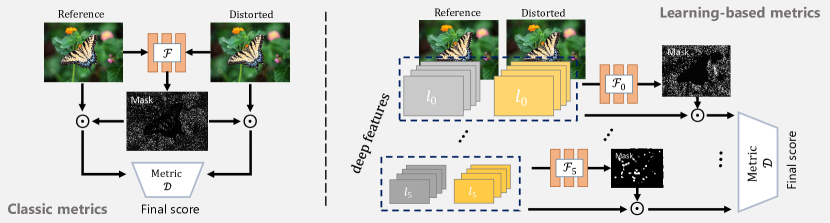
The objective of this work is not to develop a new perceptual FR-IQM; instead, we are interested in improving the quality prediction of existing metrics to align more closely with human judgment (Fig. 1). We also aim to enhance the accuracy of error map predictions by considering multiple factors such as image content, distortion levels, and distortion types. By detecting both the presence and evaluating the magnitude of visible distortion in each pixel, we aim to ensure that the metric predictions more accurately reflect the probability of a human observer detecting differences between a pair of images. In this regard, there have been several efforts toward incorporating the perceptual aspects of human vision, specifically visual masking [legge1980field, foley94human, wilson1984modified], into FR-IQM methods [lubin1995visual, Daly93, mantiuk2011hdr, mantiuk2021fovvideovdp]. In simple words, visual masking refers to the phenomenon in which certain components of an image (in our application, distortions) may be less visible to the viewer due to the presence of other visual elements in the same image. Visual masking can affect image quality perception, making some image distortions less visible to the viewer [ferwerda1997model, zeng2020overview]. However, existing visual masking models are typically hand-crafted and struggle to generalize effectively across various distortion types. Although learning a visual masking model appears to be a natural solution, the lack of reliable ground truth data for visual masking makes direct supervision impractical. In this work, we propose a self-supervised approach to predict visual masking using a dataset of images featuring a variety of distortions of different magnitudes whose quality has been evaluated in the mean opinion scores (MOS) experiment with human subjects [lin19]. In summary, our work offers the following contributions:
-
•
We propose a lightweight CNN that generates a mask for a given reference and distorted input pair. The predicted mask acts as a per-pixel weight and, when multiplied with the inputs, greatly improves the performance of the existing FR-IQMs. The incorporation of our learned mask into any FR-IQM is seamless and demands minimal computational resources. While the CNN is trained specifically for each metric, it learns a generic masking model capable of identifying various types of distortions.
-
•
We demonstrate that our masking model can be generalized to deep features and used as a per-layer feature map weight.
-
•
Our solution significantly enhances the accuracy of quality prediction for FR-IQMs across various test datasets. Furthermore, it produces per-pixel error maps that visually align more closely with human perception compared to the original FR-IQMs.
-
•
We show the potential application of our approach as a loss function for training image denoising and motion deblurring.
2 Previous work
FR-IQMs can be categorized into classical metrics, which perform the computation directly in the image space, and learning-based metrics, which leverage deep feature models to assess image quality.
Classic metrics Basic FR-IQMs, such as MSE, RMSE, and MAE, compute the per-pixel difference to quantify image distortion. While these metrics are straightforward to calculate, their consistency with human vision is typically low. Such perceptual consistency can be improved by considering relative instead of absolute error, as in PSNR and the symmetric mean absolute percentage error (SMAPE) [vogels2018denoising]. To account for the spatial aspects of the HVS, alternative metrics such as SSIM [wang04] are introduced, which consider image patches and measure local differences in luminance, contrast, and structural information. SSIM is further extended to multi-scale MS-SSIM [wang03] and complex wavelet CW-SSIM [sampat2009complex] versions that capture both global and local structural information. FSIM [zhang11] decomposes the image into multiple subbands using Gabor filters and compares subband responses between the reference and distorted images. By assuming that natural images have a specific distribution of pixel values, models based on information theory [sheikh2005information, sheikh06] measure the mutual information between images by comparing their joint histograms and taking into account the statistical dependencies between neighboring pixels. Classical metrics can offer either a single overall quality score or a visibility map indicating the distortion intensity. Watson-DCT [Watson1993], VDM [lubin1995visual], VDP [Daly93], HDR-VDP [mantiuk2011hdr], and fovVideoVDP [mantiuk2021fovvideovdp] measure either the visibility of distortions or perceived distortions magnitude, or both by considering various visual aspects such as luminance adaptation, contrast sensitivity, and visual masking. A more recent metric, FLIP [Andersson2020], emphasizes color differences, and it is sensitive to even subtle distortions by emulating flipping between the compared image pair.
Deep learning-based metrics
In recent years, research in FR-IQM has been placing greater emphasis on perceptual comparisons in deep feature space rather than image space to enhance the alignment with human judgments. Prashnani et al. [prashnani2018pieapp] are among the first to utilize deep feature models learned from human-labeled data to predict perceptual errors. Zhang et al. [zhang2018perceptual] demonstrate that internal image representations from classification networks can be used for image comparison. They propose the Perceptual Image Patch Similarity (LPIPS) index, which quantifies image similarity by measuring the distances between pre-trained VGG features. To further improve the correlation with human judgments, they learn per-channel weights for selected VGG features using their collected perceptual similarity dataset. Recognizing that simple -norm measures fail to consider the statistical dependency of errors across different locations, Ding et al. [ding20] introduce the DISTS, which aims to measure the texture and structure similarity between feature pairs by comparing their global mean, variance, and correlations in the form of SSIM. Building upon this work, A-DISTS [ding21] extended the approach to incorporate local structure and texture comparisons. Czolbe et al. [Czolbe2020] incorporate their extended Watson-DCT model [Watson1993] as a measure of VGG feature distance. Moving away from deterministic point-wise feature comparisons, DeepWSD [liao22] compares the overall distributions of features using the Wasserstein distance, a statistical measure for comparing two distributions. Nevertheless, the majority of the proposed IQMs metrics are targeted toward producing a single quality score and are not primarily designed to generate per-pixel error maps. In this regard, Wolski et al. [wolski2018dataset] employ a custom CNN model trained in a fully supervised way using coarse user marking data to predict an error visibility map that highlights the regions where distortions are more likely to be noticeable.
Recently, deep learning-based no-reference metrics (NR-IQM) such as KonCept512 [koniq10k], HYPERIQA [hyperiqa20], MUSIQ [musiq21]
and MANIQA [yang2022maniqa] have been proposed. While NR-IQM methods often report impressive performance, their practical applicability remains limited. FR-IQM metrics are still predominant in CG applications, as the reference images are typically readily available.
In this work, we extend the classic and deep learning-based full-reference metrics by introducing a learnable component trained on perceptual MOS data in a self-supervised way. By implicitly analyzing local image content, our model derives per-pixel maps that mimic visual masking, effectively modeling the visual significance of distortions.
3 Self-supervised visual masking
This section elaborates on our methodology for perceptually calibrating the existing FR-IQMs. Given a reference and distorted pair (
References
- [1] nd ) , we first learn a visual mask, , which has the same spatial dimensions as the inputs. For classical metrics (Fig. 2-left), the input
- [2] nd are sRGB images (), while for learning-based metrics such as LPIPS, DISTS, or DeepWSD, the input
- [3] nd are the VGG features extracted from the images and is the number of channels in a given VGG layer (Fig. 2-right). The predicted mask is then element-wise multiplied with
- [4] nd before being fed into an FR-IQM, . Note that, for learning-based metrics, a direct modulation of the input sRGB images by a mask would distort their content and consequently reduce the VGG performance as it is originally trained on complete, non-masked images. Our solution with VGG feature modulation draws inspiration from classic FR-IQMs [lubin1995visual, Daly93, mantiuk2011hdr, mantiuk2021fovvideovdp], where the response from hand-crafted filter banks is transduced using a fixed, perception-motivated masking model [legge1980field, foley94human, wilson1984modified]. In our approach, the response from pre-trained VGG filters is modulated with a learned per-pixel mask , where perception modeling is learned from the MOS data. We estimate the mask by utilizing a lightweight CNN denoted as , which takes both
-
[5]
nd as input. Mathematically, this can be expressed as:
M (1) -
[7]
It is important to note that the network is trained specifically for a metric . In the case of metrics such as LPIPS, DISTS, and DeepWSD, we follow their specific architecture and compute a mask for each layer using a separate , and the same mask is applied for all channels in a given layer (Fig. 2-right). The original spatial pooling is preserved for each metric, such as L1 distance in LPIPS, structural similarity in DISTS, or Wasserstein distance in DeepWSD. Since we cannot directly supervise the output of the mask generator network, we adopt a self-supervised approach to train it using an IQM dataset with a single quality score. The network’s parameters are optimized by minimizing the difference between the metric output value and human scores. Our loss is formulated as follows:
Loss (2) - [9] Here, represents the normalized mean opinion score when comparing the images
- [10] nd . As the metric response can vary in an arbitrary range, following a similar approach in [zhang2018perceptual], a small network is jointly trained to map the metric response to the human ratings.
- [11]
- [12]
3.1 Training and network details
For training, we use the KADID dataset [lin19], which comprises 81 natural images that have been distorted using 25 types of traditional distortions, each at five different levels, making roughly 10k training pairs. Note that we train our mask generator network for all the distortion categories together rather than for one specific category. We find that a lightweight CNN with three convolutional layers, each consisting of 64 channels, suffices for successful training. ReLU activation is applied after each layer, while we use Sigmoid activation for the final layer to keep the mask values in the range between 0 and 1. The computation overhead of our mask generator network is very negligible, and it takes only 12 ms to compute the mask on a 1080Ti GPU with an input resolution of . Our mapping network consists of two 32-channel fully connected (FC) ReLU layers, followed by a 1-channel FC layer with Sigmoid activation. The batch size for training is set to 4. We employ the Adam optimizer [kingma2017adam] with an initial learning rate of and a weight decay of .
| CSIQ | TID | PIPAL | ||||||||
| Metric | PLCC | SRCC | KRCC | PLCC | SRCC | KRCC | PLCC | SRCC | KRCC | |
|
|
0.900 | 0.913 | 0.740 | 0.847 | 0.789 | 0.611 | 0.651 | 0.617 | 0.441 | |
| VIF | 0.826 | 0.841 | 0.642 | 0.820 | 0.813 | 0.616 | 0.584 | 0.538 | 0.378 | |
| HDR-VDP-2 | 0.761 | 0.886 | 0.704 | 0.715 | 0.753 | 0.571 | 0.514 | 0.503 | 0.354 | |
| PieAPP | 0.827 | 0.840 | 0.653 | 0.832 | 0.849 | 0.652 | 0.729 | 0.709 | 0.521 | |
|
|
0.819 | 0.801 | 0.599 | 0.639 | 0.627 | 0.409 | 0.458 | 0.443 | 0.304 | |
| S-MAE | 0.656 | 0.697 | 0.493 | 0.498 | 0.496 | 0.347 | 0.369 | 0.365 | 0.248 | |
| E-MAE | 0.871 | 0.917 | 0.738 | 0.857 | 0.863 | 0.673 | 0.597 | 0.606 | 0.429 | |
|
\hdashline
|
0.851 | 0.837 | 0.645 | 0.726 | 0.714 | 0.540 | 0.468 | 0.456 | 0.314 | |
| E-PSNR | 0.901 | 0.910 | 0.728 | 0.855 | 0.844 | 0.656 | 0.637 | 0.629 | 0.446 | |
|
\hdashline
|
0.848 | 0.863 | 0.665 | 0.697 | 0.663 | 0.479 | 0.550 | 0.534 | 0.373 | |
| E-SSIM | 0.869 | 0.910 | 0.732 | 0.842 | 0.868 | 0.677 | 0.671 | 0.656 | 0.469 | |
|
\hdashline
|
0.826 | 0.841 | 0.642 | 0.820 | 0.813 | 0.616 | 0.584 | 0.538 | 0.379 | |
| E-MS-SSIM | 0.862 | 0.895 | 0.709 | 0.806 | 0.825 | 0.621 | 0.642 | 0.634 | 0.453 | |
|
\hdashline
|
0.731 | 0.724 | 0.527 | 0.591 | 0.537 | 0.413 | 0.498 | 0.442 | 0.306 | |
| E-FLIP | 0.871 | 0.902 | 0.715 | 0.859 | 0.858 | 0.666 | 0.621 | 0.612 | 0.434 | |
|
\hdashline
|
0.795 | 0.821 | 0.632 | 0.742 | 0.727 | 0.544 | 0.565 | 0.509 | 0.358 | |
| E-FovVideoVDP | 0.841 | 0.882 | 0.685 | 0.830 | 0.816 | 0.623 | 0.662 | 0.626 | 0.449 | |
|
\hdashline
|
0.938 | 0.952 | 0.804 | 0.853 | 0.820 | 0.639 | 0.643 | 0.610 | 0.432 | |
| E-VGG | 0.914 | 0.938 | 0.776 | 0.895 | 0.889 | 0.710 | 0.695 | 0.675 | 0.485 | |
|
\hdashline
|
0.944 | 0.929 | 0.769 | 0.803 | 0.756 | 0.568 | 0.640 | 0.598 | 0.424 | |
| R-LPIPS | 0.931 | 0.917 | 0.756 | 0.898 | 0.886 | 0.697 | 0.670 | 0.640 | 0.447 | |
| E-LPIPS | 0.922 | 0.933 | 0.771 | 0.884 | 0.876 | 0.689 | 0.705 | 0.678 | 0.490 | |
|
\hdashline
|
0.947 | 0.947 | 0.796 | 0.839 | 0.811 | 0.619 | 0.645 | 0.626 | 0.445 | |
| E-DISTS | 0.938 | 0.925 | 0.754 | 0.903 | 0.915 | 0.725 | 0.725 | 0.697 | 0.507 | |
|
\hdashline
|
0.944 | 0.940 | 0.785 | 0.808 | 0.763 | 0.573 | 0.627 | 0.606 | 0.429 | |
| E-Watson-VGG | 0.917 | 0.936 | 0.776 | 0.886 | 0.895 | 0.716 | 0.697 | 0.678 | 0.488 | |
|
\hdashline
|
0.949 | 0.961 | 0.821 | 0.879 | 0.861 | 0.674 | 0.593 | 0.584 | 0.409 | |
| R-DeepWSD | 0.955 | 0.961 | 0.823 | 0.895 | 0.88 | 0.695 | 0.654 | 0.633 | 0.449 | |
| E-DeepWSD | 0.937 | 0.937 | 0.775 | 0.905 | 0.892 | 0.710 | 0.704 | 0.672 | 0.485 | |
|
|
0.769 | 0.757 | 0.573 | 0.679 | 0.662 | 0.489 | 0.325 | 0.363 | 0.250 | |
| MANIQA | 0.874 | 0.827 | 0.642 | 0.784 | 0.760 | 0.572 | 0.404 | 0.407 | 0.276 | |
|
|
||||||||||
4 Results
In this section, we first present our experimental setup, which we use for our method evaluation and ablations of different training strategies.
4.1 Experimental setup
We employ our visual masking approach to enhance some of the classical metrics (MAE, PSNR, SSIM, MS-SSIM, FLIP, and fovVideoVDP) and recent learning-based methods (VGG, LPIPS, DISTS, Watson-VGG, and DeepWSD). Note for MS-SSIM, we used the same across all scales, while the inputs are images at different scales. Moreover, the metric called VGG is computed by simply taking the difference between VGG features for the same layers as originally chosen for LPIPS and DISTS. Deploying our masking model to PieAPP or any other metrics that create new CNN architectures from scratch is not practical as there is no intermediate component to which we can apply our masking model. Thus, our main focus remains on mainstream metrics that use features extracted from pre-trained networks for quality prediction. We assess the performance of our proposed approach on three well-established IQM datasets: CSIQ [Larson2010MostAD], TID2013 [Ponomarenko13], and PIPAL [gu2020pipal]. The first two datasets mainly consist of synthetic distortions, ranging from 1k to 3k images. On the other hand, PIPAL is the most comprehensive IQM dataset due to its diverse and complex distortions, consisting of 23k images. Each reference image in this dataset was subjected to 116 distortions, including 19 GAN-type distortions. For evaluation, following [ding20], we resize the smaller side resolution of input images to 224 while maintaining the aspect ratio. Note that rescaling is only performed on the test datasets to match the image resolution in which the MOS data were collected. Our approach does not require rescaled inputs, and all visual figures in the paper are processed in their original resolution. For each dataset, three metrics are used for evaluation: Spearman’s rank correlation coefficient (SRCC), Pearson linear correlation coefficient (PLCC), and the Kendall rank correlation coefficient (KRCC). The PLCC measures the accuracy of the predictions, while the SRCC indicates the monotonicity of the predictions, and the KRCC measures the ordinal association. The PLCC measures linear correlation, requiring both variables (metric output and MOS) to be on the same scale, hence, we mapped the metric scores to the MOS values using a four-parameter logistic function, consistent with established IQM methods [ding20, liao22]. We do not use for PLCC remapping; otherwise, we need to train a specific for each metric on a given test set. Importantly, SRCC and KRCC scores do not require additional remapping, thus directly reflecting the correlation between metric output and MOS data.
4.2 Evaluations
In this section, we present the outcome of the quantitative (agreement with the MOS data) and qualitative (the quality of error maps) evaluation of our method. We also analyze the mask content and relate it with perceptual models of contrast and blur perception. Finally, we analyze the error map prediction of different distortion levels, and we consider the potential use of our enhanced E-MAE metric as a loss in denoising and deblurring image restoration tasks.
| Loss | PSNR | SSIM | LPIPS | E-MAE | PSNR | SSIM | LPIPS | E-MAE | PSNR | SSIM | LPIPS | E-MAE | PSNR | SSIM | LPIPS | E-MAE |
|
|
34.36 | 0.94 | 0.058 | 0.0343 | 31.94 | 0.90 | 0.092 | 0.0849 | 28.82 | 0.84 | 0.163 | 3.187 | 28.02 | 0.81 | 0.182 | 4.258 |
|
|
34.37 | 0.94 | 0.055 | 0.0145 | 31.92 | 0.91 | 0.087 | 0.0263 | 28.71 | 0.84 | 0.152 | 0.790 | 27.88 | 0.81 | 0.167 | 1.035 |
|
|
||||||||||||||||
4.3 Ablations
We perform a set of ablations to investigate the impact of reduced training data in terms of distortion levels, reference image number, and distortion type diversity on the E-MAE metric prediction accuracy.
| Metric | PSNR | SSIM | LPIPS | E-MAE | |
|
|
31.70 | 0.92 | 0.1030 | 0.0192 | |
| MAE + E-MAE | 31.78 | 0.93 | 0.1018 | 0.0184 | |
|
|
| Metric Category: | noise | blur | all |
| MAE | 0.601 | 0.934 | 0.545 |
| E-MAE (noise) | 0.847 | 0.927 | 0.674 |
| E-MAE (blur) | 0.732 | 0.926 | 0.655 |
| E-MAE (noise & blur) | 0.841 | 0.936 | 0.726 |
| E-MAE (all) | 0.906 | 0.955 | 0.857 |
5 Limitations and future work
The actual visual contrast masking is the function of the viewing condition and the display size [chandler2013seven], which is often considered in the perceptual quality metrics [Daly93, mantiuk2011hdr, mantiuk2021fovvideovdp, Andersson2020] but otherwise mostly ignored. However, the effectiveness of our visual masking model is limited to the experimental setup where human scores are obtained in the KADID dataset.