Solar Cycle Observations

Abstract

We describe the defining observations of the solar cycle that provide constraints for the dynamo processes operating within the Sun. Specifically, we report on the following topics: historical sunspot numbers and revisions; active region (AR) flux ranges and lifetimes; bipolar magnetic region tilt angles; Hale and Joy’s law; the impact of rogue ARs on cycle progression and the amplitude of the following cycle; the spatio-temporal emergence of ARs that creates the butterfly diagram; polar fields; large-scale flows including zonal, meridional, and AR in-flows; short-term cycle variability; and helioseismic results including mode parameter changes.

1 Introduction

In the mid 1800s, Schwabe (1844) discovered the solar cycle by observing that sunspot numbers rise and fall over the course of roughly 11 years. This discovery likely inspired Wolfe to take daily observations of the Sun, thus beginning the crucial, historical recording of the sunspot number. See Section 2 for the history, and recent revision, of the sunspot numbers. Studies of individual ARs and their properties began with sunspot drawings and daily observations, but AR research was revolutionized by Hale (1908) who demonstrated their magnetic nature, as discussed in Section 3.

Larmor (1919) proposed that the solar magnetic fields observed by Hale and his colleagues were generated through the process of electromagnetic induction in the electrically conducting solar plasma. This idea became known as dynamo theory and its evolution as applied to the Sun and stars is discussed extensively in Charbonneau and Sokoloff (2023).

In addition to records of sunspot numbers, the area and position of sunspots has been recorded since 1874, beginning at the Royal Observatory, Greenwich and later continuing via the National Oceanic and Atmospheric Administration (NOAA). The distribution of sunspot area as a function of latitude and time revealed that two sunspot bands existed on either side of the heliographic equator and that these bands moved equatorward during the course of the solar cycle.This pattern is known as the butterfly diagram and is discussed in Section 4. One criteria of success for any dynamo model is its ability to reproduce the features of the sunspot bands, including the observed equatorward migration.

While sunspots are distinctive, visible features containing strong magnetic fields, sunspots account for less than 1 % of the solar surface area even at solar cycle maximum. Determining the larger, global-scale magnetic structure of the Sun required measurements of weaker, more spatially distributed fields (Stenflo, 1970). There is a large-scale dipole field that dominates at cycle minimum. The amplitude of this dipole is a reliable precursor for the next cycle amplitude, which is best-studied through the accumulation of small-scale flux at the poles, as discussed in Section 5.

The magnetic nature of the solar cycle is only a part of the story. The behavior of large-scale flows informs us of the variations associated with the dynamo. These plasma motions include differential rotation (radial and latitudinal), torsional oscillations, meridional flow and AR in-flows, as discussed in Section 6. Finally, short-term cycle variations and helioseismic mode parameter changes are mentioned in Sections 7 and 8, respectively.

This review paper is a result of an International Space Science Institute Workshop titled “Solar and Stellar Dynamos: A New Era” held in June, 2022. Discussions in this review paper are intentionally brief and may not be comprehensive, since the purpose is to introduce the observations that have inspired the up-to-date research summarized in the other papers that are part of this series, Space Science Reviews:219.

2 Sunspot Number

The sunspot number (SN) is a synthetic (not physical) quantitative index of solar activity, which is historically widely used because of its simplicity and long (more than 400 years) available dataset. The SN is not equal to the number of sunspots (denoted as $s$ below) but includes also the weighted number of sunspot groups $g$, using the formula introduced by Rudolf Wolf in the middle of the 19th century:

$$SN=k\cdot(10\cdot g+s),$$ (1)

where $k$ is a scaling factor reducing the data quality (related, e.g., to the quality of the instrumentation used) of individual observers to that of the reference one (usually Rudolf Wolf or Alfred Wolfer are considered as the reference observers). A single spot on the Sun ($s=1$) is counted as a single sunspot group leading thus to SN=11. The classical Wolf’s method uses observations of only one, so-called primary observer for each day. If the primary observer’s data was not available for a day, secondary, tertiary, etc. observers were used, but always only one per day (see Waldmeier, 1961). This makes the SN series easy to calculate but leaves no way to verify it nor to estimate its uncertainty. This forms the so-called Wolf or Zürich SN series (WSN or $Z$). The WSN was continuously produced by Zürich Observatory using roughly nearly the same, reproducible, techniques. The main shortcoming of the WSN is that it is not transparent and cannot be presently revisited, corrected or verified, since only the final product has been published while raw data were hand-written in log books. These old log books are being digitized now making it potentially possible to revise the WSN in the future (Friedli, 2020).

The production of the SN series was was ceased in the 1980s in Zürich and smoothly transmitted to Brussels (Sunspot Index and Long-term Solar Observations project, SILSO – http://sidc.be/silso), where it is continued in the form of the International Sunspot Number, ISN (Clette et al, 2007). SILSO continues using the same formula (Eq. 1) for ISN but changed the methodology so that not only a single primary observer’s data, but a weighted sum of all available data are used for each day.

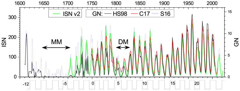
Figure 1: Annual sunspot activity for the last centuries according to different recent reconstructions: International sunspot number (ISN) series version 2 (green ISN v2 curve, left axis) obtained from SILSO; Sunspot group number (GN, right axis), according to HS98 – Hoyt and Schatten (1998); C17 – Chatzistergos et al (2017); S16 – Svalgaard and Schatten (2016). Standard (Zürich) cycle numbering is shown between the panels. Approximate dates of the Maunder minimum (MM) and Dalton minimum (DM) are labeled within the figure. Modified after Usoskin (2023).

For more than a century, the WSN was the “gold standard” in solar studies, but then several problems were identified, including difficulties maintaining consistency with new data. Hoyt and Schatten (1998) developed a new index, called Group sunspot number, GSN (or GN), based on a weighted sum of the number of sunspot groups reported for each day by all possible observers. They neglected the number of individual spots as less reliably detected. Hoyt and Schatten (1998) added a lot of new data not known to R. Wolf and his successors and, most importantly, published the entire database of raw data, making it possible to assess the uncertainties and add or revise the data if needed. This also allows evaluation of the related uncertainties. The database of individual historical observations is continuously updated at http://haso.unex.es/?q=content/data (Vaquero et al, 2016).

After a careful study, several issues have been found in the WSN/ISN dataset, such as discontinuous transitions between different observers or changed methodology (e.g., Leussu et al, 2013; Clette et al, 2014). These obvious discontinuities have been ad-hoc corrected in the revised ISN series, which have been also normalized to A. Wolfer as the reference observer – the latter leads to a scaling factor of 1.667 with respect to the classical WSN. This forms the ISN version 2 dataset which is considered as a current version (Clette and Lefèvre, 2016), as shown by the green curve in Figure 1. A new revision of the ISN, version 3, is pending in the near future as the first consensus dataset using the best of our present-day knowledge.

Independently of the WSN/ISN, the methodology has been revisited for the GSN series, starting from the raw-data database. Several new approaches have been developed in this direction. One was made by Svalgaard and Schatten (2016) who performed a daisy-chain ‘backbone’ GSN composition following the classical scheme of linearly scaling individual observers between each other (blue dotted curve in Figure 1). The daisy-chain approach was further improved by Chatzistergos et al (2017) who accounted for non-linear relations between data from overlapping observers and composed a new GN series (red curve in Figure 1). A new approach has been developed recently (Usoskin et al, 2016; Willamo et al, 2017) that uses the active-day (days with at least one sunspot observed) fraction as the metrics of the minimum size of sunspot group that could be detected by an observer due to instrumentation and seeing conditions.

Of special interest is the level of solar activity during the Maunder minimum of 1645 – 1715 (Eddy, 1976): while the present paradigm is that it was nearly sunspot free (e.g., Usoskin et al, 2015; Carrasco et al, 2021), some estimates predict low but still significant sunspot activity (Svalgaard and Schatten, 2016; Zolotova and Ponyavin, 2015). However, a consistent analysis of the multitude of other data, such as cosmogenic isotopes, auroral records, solar eclipse observations, confirms the very low level of solar activity during the Maunder minimum (e.g., Usoskin et al, 2015; Asvestari et al, 2017; Carrasco et al, 2021; Hayakawa et al, 2021), implying particularly that the reconstruction by Svalgaard and Schatten (2016) is too high in the 18th century.

Thus, at present there is a zoo of SN and GN reconstructions, as shown in Figure 1. Generally, they are all consistent after about 1870 but somewhat disagree for the period between 1749 – 1870, with the difference being indicative of the systematic uncertainties. The GSN series by Hoyt and Schatten (1998) and by Svalgaard and Schatten (2016) can be considered as conservative lower and upper bounds, respectively, while other models lie between them. A consensus-based SN reconstruction is presently not available but it is under consideration by the research community.

3 Active Regions (ARs)

An AR is identified as a dark feature observed in the solar photosphere in white light observations. ARs contain strong, bipolar magnetic fields and are associated with sunspots. In this section, we discuss observational aspects of ARs that contribute to our understanding of the solar cycle. For a review of the origins of ARs and their emergence process, see Weber et al (2023).

3.1 Hale’s Law

Hale (1908) realized that magnetic fields were the cause of sunspots after observing the Zeeman splitting of a spectral line from the light originating in a sunspot. He also noted that sunspots appeared in pairs of positive and negative magnetic polarity and that the leading polarity (with respect to rotation) in each hemisphere changes from one sunspot cycle to the next. This is known as Hale’s polarity law, see Figure 2. While Hale’s law is straightforward, it has profound implications for the solar dynamo. It implies that the large-scale organization of the magnetic field in the interior is mostly toroidal (East-West) in orientation and oppositely directed on either side of the equator. ARs adhere to Hale’s law $\sim$92-95 % of the time (Wang and Sheeley, 1989; McClintock et al, 2014; Li, 2018; Muñoz-Jaramillo et al, 2021).

3.2 Flux Ranges and Lifetimes

ARs are part of a spectrum of magnetic bipoles that emerge into the photosphere and have a smooth, distribution function in regards to size and total absolute flux values ranging from 10¹⁸ to 10²³ Mx. Ephemeral regions are smaller, short-lived regions with flux less than 1 $\times$ 10²⁰ Mx and have a lifetime of hours, i.e., shorter than a day (Hagenaar et al, 2003). Small regions appear as pores with flux in the range of 1 $\times$ 10²⁰ to 5 $\times 10^{21}$ Mx (van Driel-Gesztelyi and Green, 2015). Larger sunspots develop well-defined penumbra and have $5\times 10^{21}$ to several $\times 10^{23}$ Mx. They live on the order of several weeks to several months. Typically, the flux emergence period is 15 – 30 % of the total lifetime (van Driel-Gesztelyi and Green, 2015), with most ARs fully emerged within 3 – 5 days (Harvey-Angle, 1993; Norton et al, 2017) and an average emergence time of $\sim$2 days (Weber et al, 2023). After flux emergence, there is a plateau of stability before the flux begins to decay.

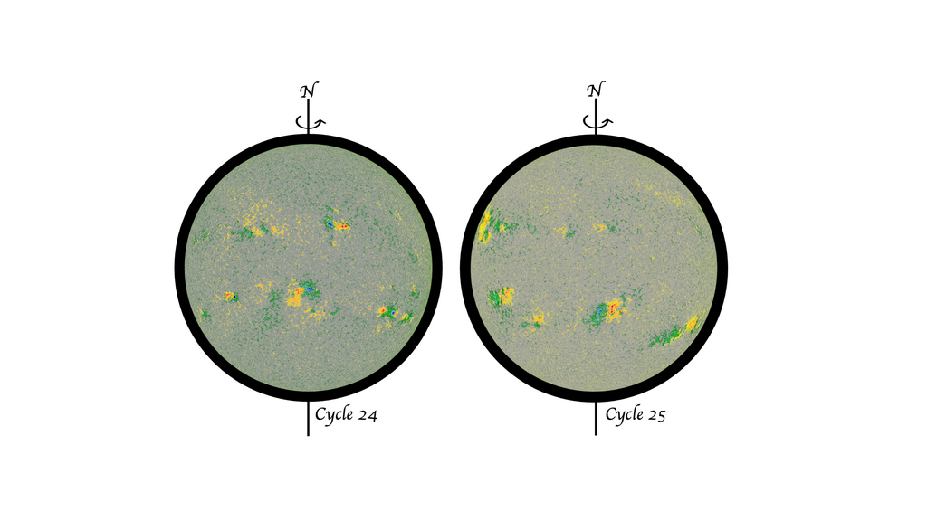
Figure 2: (Top) Hale’s law describes how bipolar magnetic regions in one hemisphere tend to have the same leading magnetic polarity while those in the other hemisphere have the opposite leading polarity. This leading polarity switches from one Solar Cycle to the next, i.e., cycle N (N+1) shows the expected polarity for Cycle 24 (25). The average tilt angles between the magnetic polarities, depicted by red lines, increase with increasing latitudes. (Bottom) HMI magnetograms from Cycles 24 (2012.04.21) and 25 (2022.05.15) show the manifestation of Hale’s and Joy’s law on any given day with orange-red (green-blue) colors identifying the location of negative (positive) polarity.

3.3 Tilt Angles

Bipolar sunspot pairs are, on average, oriented so that the leading sunspot is closer to the equator than the following sunspot, see Figure 3 for an example, and also the red lines connecting the bipolar sunspot pairs in Figure 2, with the angle being a measure of the orientation of the bipolar magnetic region’s axis with respect to the East–West direction. On average, the tilt angles increase with latitude, and this trend was named “Joy’s Law” by Zirin (1988), see Figure 3. Tilt angles are crucial in flux-transport dynamo models where it plays a role in the formation and evolution of polar fields (see, e.g., Wang and Sheeley, 1991; Dikpati and Charbonneau, 1999a). Tilts serve as an observable feature of the conversion of toroidal magnetic field into poloidal, i.e., the $\alpha$-effect, and the reversal of axial dipole between cycles (Cameron et al, 2018).

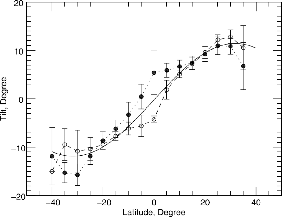
Figure 3: The majority of ARs emerge in nearly an E-W orientation with a tendency for the leading spot (with respect to rotation) to be closer to the equator. A southern hemisphere AR from Cycle 24 is shown (top) as observed in SDO/HMI intensity and magnetogram. (Bottom) The binned, mean tilt of magnetic bipoles as a function of latitude from Cycles 15$-$24 from Mt. Wilson Observatory daily sunspot drawings with magnetic polarity indicated. RMS of mean tilt shown as error bars with even (open circles, dashed line) and odd cycles (filled circles, dotted line) as well as a fit to all data (solid line) of the form $\gamma=0.2\sin(2.8\theta$) where $\gamma$ is the tilt angle and $\theta$ is latitude. This form of Joy’s law captures the inflection point in tilt values at mid-latitudes. Lower image reproduced with permission from Tlatova et al (2018), copyright from Springer Nature.

There are two dominant, physical explanations for the origin of Joy’s law. First, as proposed by Babcock (1961), the tilt angle observed in the photosphere reflects the directional components of the global magnetic field at depth and is a direct consequence of the “winding up” of the poloidal field in the solar interior. Second, Wang and Sheeley (1991) propose that Joy’s law is a result of the Coriolis force acting on flows within the flux tube as it rises through the convection zone.

Joy’s law is a statistical law and only becomes obvious after much averaging. A study by Wang and Sheeley (1989) with over 2500 bipolar magnetic regions reported that 16.6 % had no measurable tilts, 19 % were anti-Joy, 4.4 % were anti-Hale. That is 39.9 % of regions that were not obeying Joy’s law. The data are so noisy that Joy’s law cannot be recovered for Cycle 17 (Cycle 19) in the northern (southern) hemisphere, respectively (McClintock and Norton, 2013) The scatter is thought to have a physical origin, the buffeting of flux tubes by convective motions (Fisher et al, 1995; Weber et al, 2011). In addition to the high scatter of tilt angles, the expansion of the sunspot group along its major axis is observed with the possibility of differential rotation acting on the poleward and equatorward spots accordingly (Gilman and Howard, 1986; Schunker et al, 2020).

Simulations of thin flux tubes rising through the convection zone with the Coriolis force acting on flows within the flux tube have been able to recreate both Joy’s law and its scatter (D’Silva and Choudhuri, 1993; Fan, 2009; Weber et al, 2011) with scatter increasing for flux tubes that spend a longer time rising. Results from 3D dynamo models show some promise of producing bipolar magnetic regions that adhere to Hale and Joy’s law (Nelson et al, 2013); there is certainly no consensus as to which models most accurately represent solar conditions and recreate tilt angle distributions.

Various forms of Joy’s law are reported in the literature including the following where $\gamma$ is the tilt angle and $\theta$ the latitude:

$$\sin\gamma=m\cdot\sin\theta+c,$$ (2)

$$\gamma=m\cdot\theta+c,$$ (3)

$$\gamma=m\cdot\sin\theta+c,$$ (4)

$$\gamma=m\cdot\sin(k\cdot\theta),$$ (5)

The reported best-fit values for slope, $m$, and intercept, $c$, depend on the solar cycle, instrument, type of data (white-light or magnetogram), and sampling techniques used for the determination of the tilt angles. Note that some researchers force the fits through zero, $c=0$, while others allow a $y$-intercept that is non-zero. For a few examples, Wang and Sheeley (1991) report Joy’s law in the form of Equation 2 with $m=0.48$ and $c=0.03$, Norton and Gilman (2005) use Equation 3 with $m=0.2$ and $c=0.2$, Tlatova et al (2018) uses Equation 5 with $m=0.2$ and $k=2.8$. Li (2018) comprehensively reports fits to the forms of Equations 2 – 4. These are only a few examples, as it is beyond the scope of this review to report an all-inclusive list of Joy’s law fits.

A list of observational aspects of tilt angles are as follows:

• the dependence on latitude differs between cycles and hemispheres (Dasi-Espuig et al, 2010; McClintock and Norton, 2013; Tlatova et al, 2018);

• there is evolution as the AR emerges and decays so the time of measuring a tilt angle matters (McClintock and Norton, 2016; Schunker et al, 2020);

• scatter is higher during the first day of emergence (Schunker et al, 2020),

• the value tends to settle near the end of emergence (Stenflo and Kosovichev, 2012; Schunker et al, 2020);

• there are conflicting reports as to whether the tilts show a dependence on magnetic flux as predicted in thin flux tube modeling (Fisher et al, 1995; Stenflo and Kosovichev, 2012; Jiang et al, 2014; McClintock and Norton, 2016; Schunker et al, 2020);

• the scatter in the tilt values has a dependence on flux but not latitude (Fisher et al, 1995);

• the mean and median tilts of regions near the equator are not zero indicating that forcing a fit for Joy’s law through the origin may be unphysical,

• an inflection point in the fit of tilts as a function of latitude occurs around $30^{\circ}$ in both hemispheres (Tlatova et al, 2018);

• the smallest bipoles appear to have negative tilts (Tlatov et al, 2013);

• and the anti-Hale regions may not simply be the tail of the distribution of tilt angles as Muñoz-Jaramillo et al (2021) reports they prefer an east-west orientation and have a distribution distinct from the ARs that follow Joy’s law.

Improvements in tilt angle measurements and databases is ongoing work. Traditional determinations of Joy’s law have been based on white-light images because magnetograms only became routinely available in the mid-1960s. White-light studies yield median tilt angles that are smaller and increase less steeply with latitude (lower slopes) than those obtained from magnetic data as shown by Wang et al (2015), who also pointed out that a substantial fraction of tilts determined from white-light data were erroneous since they were from sunspots of the same polarity. In addition, if plage is included in the calculation, the tilt angle is usually higher. Given the errors in tilt angle determinations prior to routine magnetograms, and inconsistent methodologies (i.e., tilt angles determined including only umbra versus those determined using umbra, penumbra and plage), it is not clear if long-term trends of tilt angles using only white-light data are valid.

An anti-correlation between area-weighted mean tilt angles (normalized by latitude) and cycle strength was shown by Dasi-Espuig et al (2010) for cycles 15-21, indicating that the surface source for the poloidal field becomes weaker for stronger cycles, potentially limiting the strength of the next cycle, and providing a feedback mechanism (“tilt-quenching”) that prevents runaway solutions to the cycle amplitude. However, McClintock and Norton (2013) could only recover the Dasi-Espuig et al (2010) result for the Southern hemisphere, not the Northern, and the Cycle 19 outlier value dominated the fit for the Southern hemispheric data. Nevertheless, non-linear feedback mechanisms that affect average tilt angles appear effective. Surface flux-transport modeling by Cameron and Schüssler (2012) and Jiang et al (2010) incorporated the effect of AR inflows into surface flux transport models and found that strong cycles produce strong in-flows which result in a lower tilt angle and decreased resulting axial dipole moment.

3.4 Rogue Active Regions

The progression of any solar cycle, including the polarity reversal and gradual strengthening of the polar caps responsible for the axial dipole moment, is punctuated by the appearance of unusually influential, or rogue, ARs. The term “rogue AR” was coined by Nagy et al (2017) who reported that a single rogue bipolar magnetic region in their simulations was found to have a major effect on the development of subsequent solar cycles, either increasing or decreasing the amplitudes, and in extreme cases, triggering a grand minimum. Nagy et al (2020) then proposed the AR Degree of Rogueness (ARDoR) quantity that is the difference between the final contribution to the axial dipole moment from an individual AR and an ideal contribution from a region at the same latitude that has an expected tilt angle prescribed by Joy’s Law and separation of opposite polarity footpoints typical for an AR of similar flux. Meaning, a region is defined as rogue when its contribution to the final axial dipole moment is significantly different from an average active region emerging at the same latitude.

Petrovay et al (2020) formulated an algebraic method that consists of summing the ultimate contributions of individual ARs to the solar axial dipole moment at the end of the cycle. Nagy et al (2020) performed a statistical analysis of a large number of simulated activity cycles and ranked the ARs from most to least influential depending on their contribution to the final axial dipole moment. The model by Lemerle and Charbonneau (2017) used in the simulation couples a conventional surface flux transport (SFT) 2D simulation defined over a spherical surface with a 2D axisymmetric flux transport dynamo (FTD) simulation defined in a meridional plane (Charbonneau et al, 2005). In this hybrid 2$\times$2D Babcock-Leighton dynamo model, the SFT component provides the surface poloidal source term for the FTD simulation, while the FTD component provides the magnetic emergence events input to the SFT simulation (Charbonneau et al, 2005; Nagy et al, 2017). They showed that the top 50 influential ARs of any given cycle are sufficient to reproduce the final dipole moment of that cycle. Rogue ARs have a variety of characteristics but their rogueness is commonly determined by having one or more of the following characteristics: a very large amount of flux ($\Phi>1\times 10^{22}$ Mx); an abnormal tilt angle such as one that is anti-Joy or anti-Hale (90–180^∘ away from Joy’s law); an unusually large separation distance between the polarities ($>$ 70 Mm); or being very close to the equator.

4 The Butterfly Diagram

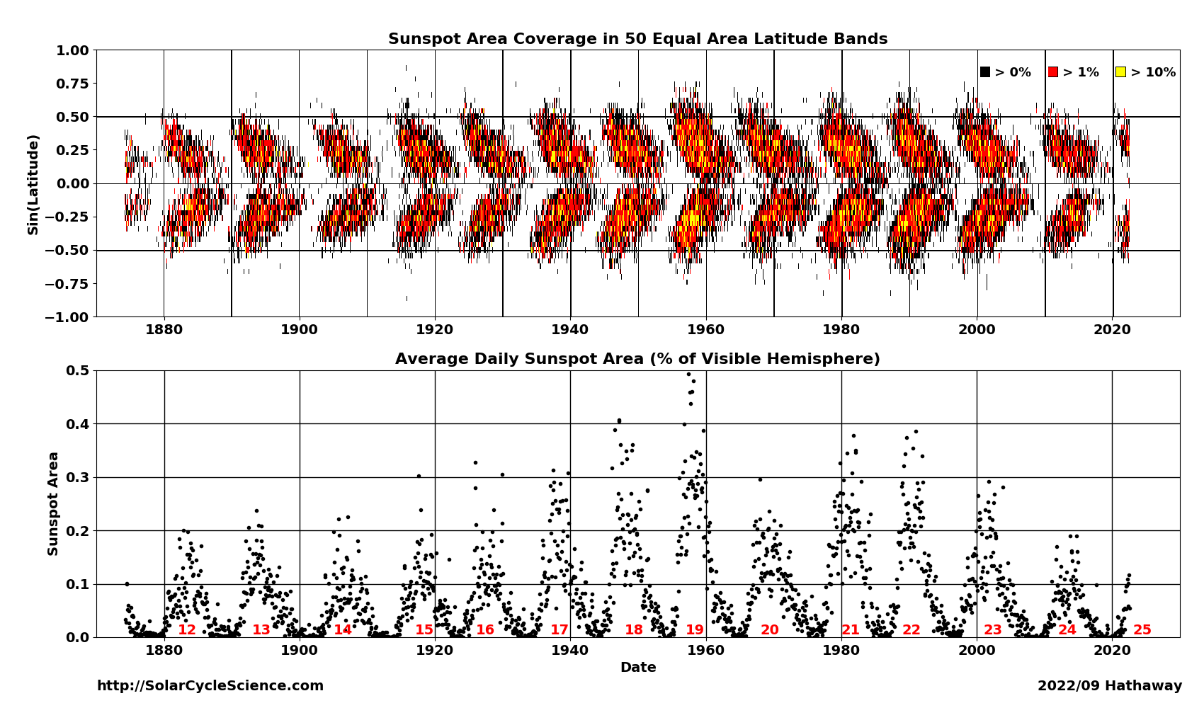
Figure 4: Butterfly diagram shows sunspot area from the Royal Greenwich Observatory, color coded as a percentage of the solar disk, plotted as a function of time and sine latitude (top panel). For reference, the total sunspot area is also plotted as a function of time (lower panel). Figure courtesy D.H. Hathaway via www.solarcyclescience.com.

When the location of sunspots or ARs are plotted as a function of latitude and time, a striking pattern emerges that resembles butterfly wings. This so called “Butterfly Diagram”, first depicted by Maunder (1904), shows bands of sunspot activity in both the Northern and Southern hemispheres. Modern depictions include a third dimension, the fractional area of the Sun covered by sunspots, see Figure 4. Inspection of the butterfly diagram reveals that early in the cycle, ARs begin emerging at mid-latitudes (approximately 30 degrees) and as the cycle progresses the emergence moves closer to the equator. This equatorward progression of AR emergence is known as Spörer’s Law (Maunder, 1903). Stronger cycles tend to begin emergence at higher latitudes than weaker cycles. The latitudinal width of the “Butterfly wings” also changes over the course of the cycle and is proportional to the strength of the solar cycle (Ivanov and Miletsky, 2011), producing a tapering of the wings at both the start and the end of the cycle. Typically the cycles overlap in time by about one – two years, with the new cycle beginning at mid-latitudes before the previous cycle has finished. However, this overlap is proportional to the strength of the following cycle such that the weakest cycles have little to no overlap with the previous cycle. Asymmetry between the northern and southern hemispheric cycle progression was noted by Sporer (1894) and Maunder (1904) with unequal sunspot activity persisting for several years. Norton et al (2014) showed that the hemispheric asymmetry never had more than a 20% difference in the amplitude of sunspot number or sunspot area. Nor was the time lag (measured by time of polar reversal, cycle maximum or minimum in each hemisphere) more than 20 % of the entire cycle length. In other words, the hemispheres are strongly coupled - to within $\approx$80 %.

While the traditional Butterfly Diagram is created in statistical manner by plotting the sunspot area as a function of latitude and time, a similar plot can be created by plotting the longitudinally averaged magnetic field instead (Harvey, 1994). This “Magnetic Butterfly Diagram”, see Figure 5 reveals several other characteristics of the solar cycle. Most notable are the appearance of Joy’s Law and Hale’s law. Each wing displays predominantly leading polarity on the southern edge and the opposite following polarity predominantly on the northern edge (Joy’s Law). The wing polarity is opposite across hemispheres and switches from one cycle to the next (Hale’s law). In addition to the butterfly wings, streams of flux can be seen emerging from the wings and moving towards the poles. They are most prominent during solar cycle maximum and are dominated by the following sunspot polarity flux for that cycle (though intermittent leading-sunspot polarity streams are also present). These streams are a signature of the pole-ward meridional flow transporting residual AR flux to the polar regions. This process forms strong flux concentrations at the poles, i.e. the polar fields, that reverse polarity near the time of solar maximum.

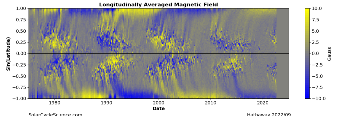
Figure 5: The magnetic butterfly diagram shows the latitudinal distribution of the magnetic field as a function of time. The magnetic field is averaged over all available longitudes and over each Carrington Rotation using data from SOLIS/MDI/HMI. The color indicated the sign of the polarity, with yellow (blue) for positive (negative) radial magnetic fields. Figure courtesy D.H. Hathaway via www.solarcyclescience.com.

5 Polar Fields

During solar minimum, the Sun’s magnetic field resembles that of a dipole, with opposite polarity magnetic field concentrations at the poles. This dipolar magnetic field acts as the seed field for the solar cycle described in Charbonneau and Sokoloff (2023); Cameron and Schüssler (2023).

The Sun’s polar magnetic fields can be measured by averaging the magnetic field strength over the polar cap to get the flux density over each polar region or by calculating the axial dipole moment of the magnetic field configuration. The latter provides a single value for the state of the Sun’s global magnetic field as a whole, while the former provides additional information about the differences between the North and South hemispheric polar magnetic field.

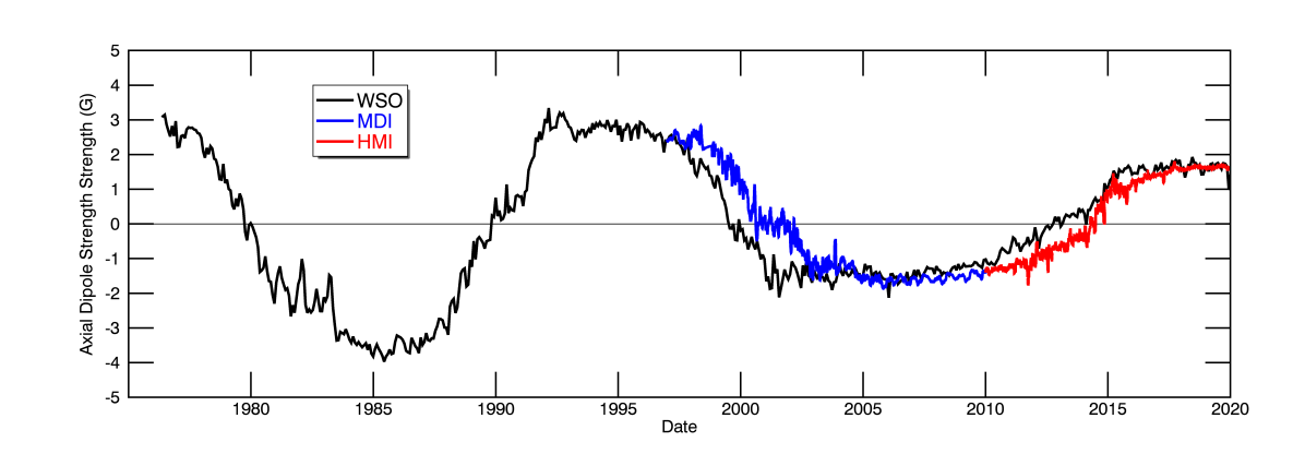
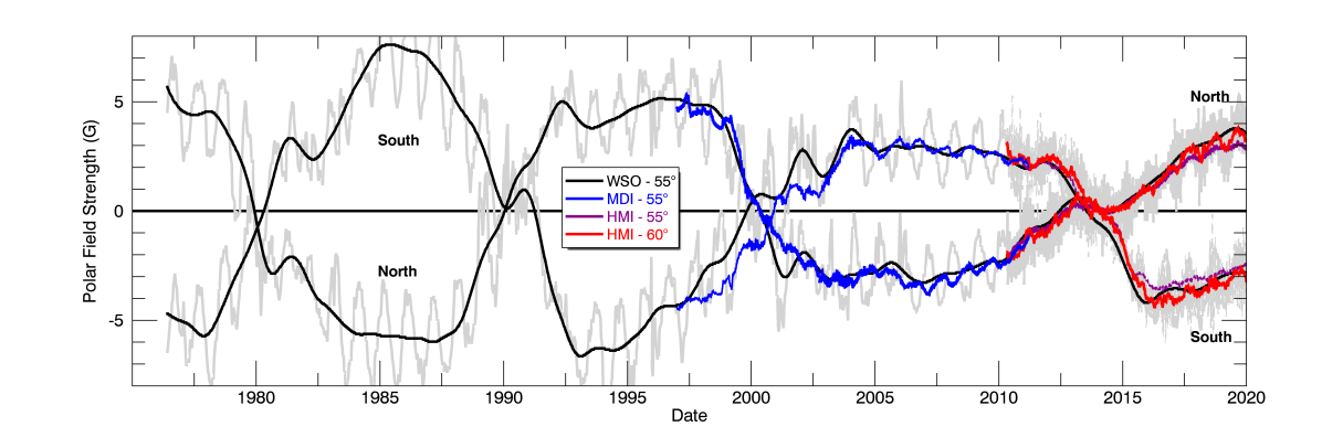
Figure 6: The Sun’s polar fields measured by the axial dipole moment (top) and by the average field strength over the polar caps (bottom). Data is shown from WSO in black, SOHO/MDI in blue, and SDO/HMI in purple and red. WSO and MDI averaged polar fields are measured from $55^{\circ}$ and above, while HMI is shown for both $55^{\circ}$ and $60^{\circ}$ (purple and red) and above. The polar fields are smoothed over 13 Carrington Rotations (for reference, the unsmoothed WSO and HMI measurements are shown in grey, highlighting the annual signal caused by the changing inclination of the Sun over Earth’s yearly orbit).

The Wilcox Solar Observatory (WSO) has been measuring the Sun’s line-of-sight magnetic field daily since 1976 and has provided measurements of both the polar field strength and the axial dipole since that time (Svalgaard et al, 1978; Hoeksema, 1995), and the axial dipole component is shown as a black line in Figure 6 (top panel). The axial dipole moment is an integrated quantity that measures the axisymmetric component of the large-scale photospheric magnetic field. The polar field strength, bottom panel in Figure 6, is defined as the flux density of the magnetic field above a specific latitude. For WSO this is limited by the spatial resolution and taken to be the line of sight field strength measured in the highest-latitude pixel, which is taken to be between 55^∘ and the poles (but the actual latitude range varies with the Earth’s orbit). Space based missions have a better resolution and in the case of HMI calculate the polar fields as the inferred radial component of the magnetic field measured at 60^∘ and above (Sun et al, 2015). While the improved resolution does mitigate the projection effects, a residual annual oscillation (gray lines in the bottom panel in Figure 6) is evidence that there is still uncertainty in these measurements due to the poor viewing angle. While the flux density over each polar region offers insight into hemispheric asymmetries, the innate ambiguity associated with this measurement may make the axial component of the Sun’s magnetic dipole a better metric for solar cycle prediction (Upton and Hathaway, 2014b).

The polar fields are out of phase with the sunspot number, with the reversal occurring near the time of solar cycle maximum. The peak in the polar field strength typically occurs at or just before solar cycle minimum. The amplitude of the Sun’s polar fields (as measured by the axial dipole or by the field strength over the polar cap) at the time of solar cycle minimum are proportional to the amplitude of the next solar cycle. Consequently, the amplitude of the polar fields at the time of cycle minimum have proven to be successful predictors of solar cycle amplitude (Schatten et al, 1978; Svalgaard et al, 2005; Petrovay, 2010; Muñoz-Jaramillo et al, 2013; Bhowmik et al, 2023). This can be understood in terms of the dynamo model proposed by Babcock (1961) and extended by Leighton (1964). For a detailed account of the Babcock-Leighton model, see Charbonneau and Sokoloff (2023) and Cameron and Schüssler (2023).

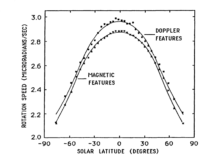
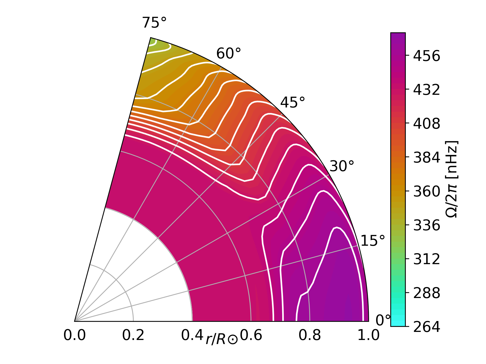
Figure 7: Top: Differential rotation measured by feature tracking (from Snodgrass and Ulrich, 1990, ©the AAS, reproduced by permission). Bottom: Solar rotation profile from 2D inversions of HMI helioseismic observations, averaged from 2010 to 2022, prepared by the authors for this review.

6 Flows

The observed large-scale flows of the Sun — differential rotation, torsional oscillations, meridional circulation, large-scale convection and the recently observed inertial modes — provide a set of measurements that characterize the solar convective processes. For a detailed account of the plasma flows in the Sun, including Rossby waves and inertial modes, see Hotta et al (2023). Herein, we introduce the fundamental observations of these flows.

6.1 Solar Rotation Profile

The mean solar rotation profile is well known. At the surface the latitudinal differential rotation can be measured by tracking features such as sunspots, revealing that the rotation rate is highest at the solar equator and decreases towards the poles (Figure 7, top). A comprehensive review of these measurements has been made by Beck (2000). Helioseismology (see, for example, Thompson et al, 1996; Schou et al, 1998; Larson and Schou, 2018) has revealed the interior rotation profile (Figure 7 bottom). It features a near-surface shear layer (sometimes abbreviated as NSSL) where the rotation rate increases with depth down to about $0.95\,{\mathrm{R}}_{\odot}$. Below this layer, latitudinal differential rotation persists through the bulk of the convection zone, approximately constant on radial lines although the isorotation contours tend to lie at about a 25-degree angle to the rotation axis over a wide range of latitudes (Gilman and Howe, 2003). There is another shear layer or “tachocline” at the $0.71\,{\mathrm{R}}_{\odot}$ base of the convection zone, which is narrower in reality than it appears in most helioseismic profiles due to the finite resolution of the inversions; the consensus (see Table 2 of Howe, 2009, and references therein) is that the thickness is around $0.05\,{\mathrm{R}}_{\odot}$, but at least one estimate (Corbard et al, 1999) puts it as low $0.01\,{\mathrm{R}}_{\odot}$. Below the tachocline, in the radiative interior, there is roughly rigid rotation down to the limits of reliable measurement at around $0.2\,{\mathrm{R}}_{\odot}$. (e.g. Eff-Darwich and Korzennik, 1998; Couvidat et al, 2003), although the former authors note that it is possible that the core is rotating somewhat faster than the bulk of the radiative interior).

Figure 8: The torsional oscillation in Mount Wilson surface Doppler observations, adapted from Ulrich et al (2022) under the CC BY 4.0 license.

6.2 Zonal Flows: Torsional Oscillations

The solar rotation profile is modulated by a pattern of bands of faster- and slower-than-average rotation, which can be considered respectively as prograde or retrograde flows, and which migrate in latitude in synchrony with the solar cycle (see Figures 8 and 9). This pattern, revealed when a temporal average is subtracted from the rotation rate at each latitude, was first observed, and dubbed the “torsional oscillation”, by Howard and LaBonte (1980) in surface Doppler observations from the 150 ft tower at the Mount Wilson Observatory. The Mount Wilson observations continued until 2013, and Figure 8 from Ulrich et al (2022) shows the pattern over three solar cycles. The main feature is the band of faster rotation in each hemisphere that moves from mid-latitudes towards the equator between one solar minimum and the next; as pointed out by Howard and LaBonte (1980), the latitude of maximum flux falls close to the edge of this belt. These flows are relatively weak compared to the mean solar rotation, with amplitudes close to the surface of less than ten meters per second, or a fraction of a per cent of the equatorial rotation rate.

Figure 9: Zonal flow map from helioseismic inversions of GONG (1995 – 2022), MDI (1996 – 2010), and HMI (2011 – 2022) data, at a target depth of $0.99\,R_{\odot}$, with a temporal mean over the whole dataset subtracted at each latitude. Note that $\delta\Omega$ here is the same quantity as $\delta\omega$ in Figure 8. Reproduced from Howe et al (2022) under the CC BY 4.0 license.

The flow patterns were seen in helioseismic data in the rising phase of Solar Cycle 23 by Schou (1999), and Howe et al (2000) found that the patterns penetrated at least 0.08 solar radii into the convection zone; subsequent work, for example by Vorontsov et al (2002), suggested that the variation in rotation involves most of the bulk of the convection zone. A strong band of faster flow migrating from mid-latitudes towards the poles early in Solar Cycle 23 was reported by Antia and Basu (2001).

Because the mid-latitude rotation begins to speed up before significant surface activity is seen, the flow pattern towards the end of one solar cycle can give some indication of the timing of the onset of the following one, as reported by Howe et al (2009) for Cycle 24 and Howe et al (2018) for Cycle 25. In particular, the time at which the main belt of faster rotation reaches a latitude of around 25 degrees seems to coincide with solar activity becoming widespread in a new cycle. The strong poleward branch seen in Cycle 23 was not repeated in Cycle 24 (Howe et al, 2013). This seems to be associated with small but significant deceleration at higher latitudes, possibly related to the weaker polar fields in Cycle 24 (Rempel, 2012). Figure 9 shows the flow residuals from inversions of GONG, MDI, and HMI data, as reported by Howe et al (2022). We note that the global helioseismic inversions can only show the North–South symmetric part of the flow pattern, while the surface measurements and those from local helioseismology (e.g. Komm et al, 2018; Lekshmi et al, 2018) can distinguish the two hemispheres. The relationship between the flow pattern and magnetic butterfly diagram is complex, but Lekshmi et al (2018) found that the hemispheric asymmetry of the flows is related to, and is a leading indicator of, the magnetic asymmetry; asymmetry in the flows is seen in advance of the corresponding asymmetry in the magnetic activity.

6.3 Meridional Flows

The solar meridional flow is the North-South motion of the plasma. At the surface this flow plays a critical role in the solar dynamo by transporting residual flux from ARs to the poles in order to generate the magnetic field to initialize the next solar cycle. This plasma flow moves from the equator to the poles in each hemisphere with an amplitude of $\sim 10-20$ m s^-1. The meridional flow is 1-2 orders of magnitude weaker than the differential rotation (relative velocities of $\sim 200-250$ m s^-1) and the convective flows (velocities of $\sim 500$ m s^-1 for supergranules and $\sim 3000$ m s^-1 for granules), making it the most challenging plasma flow to measure. The meridional flow is typically measured in the same manner as (and along with) the differential rotation (e.g., Doppler imaging, helioseismology, tracking techniques, etc.). Characterizing this flow is particularly challenging because independent measurement techniques can often give very different measurements, thought to be a consequence of the different depths sampled by each technique. For an in depth review, see Hanasoge (2022) and references therein.

High resolution continuous magnetic data from space-based observatories (i.e., SOHO/MDI and SDO/HMI) have ushered in a new era, paving the way for meridional flow measurements with unprecedented spatial and temporal resolution, revealing that the amplitude and structure vary with the solar cycle (Gizon, 2004; González Hernández et al, 2008a; Hathaway and Rightmire, 2010). The meridional flow measured by magnetic pattern tracking (Hathaway et al, 2022) for the last two solar cycles (see Figure 10) shows that the meridional flow is the strongest at solar cycle minimum and weakens during solar minimum. This weakening of the meridional flow was more pronounced during the stronger Solar Cycle 23 than it was for the weak Solar Cycle 24. The relative magnitude of this cycle dependent change in the flow speed is illustrated in the left panel of Figure 11. This modulation of the meridional flow by the presence of ARs may serve as a nonlinear feedback mechanism for regulating the solar cycle, as described in the next section.

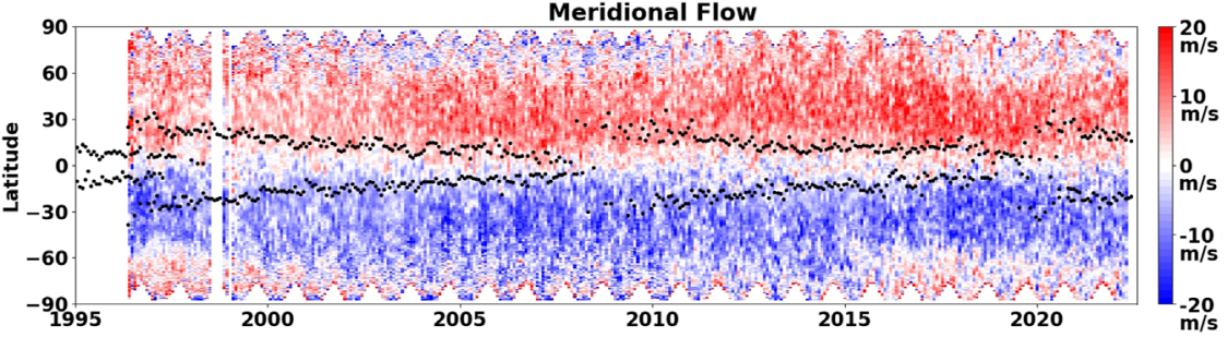
Figure 10: The evolution of the meridional flow measured by magnetic pattern tracking of MDI/HMI data over the last two cycles is shown in the left panel (adapted from Hathaway et al (2022)).

Another aspect of the meridional flow is the quite contentious existence of the high-latitude equatorward flows, sometimes referred to as polar counter-cells. If present, these flows would have implications for the build up of the polar fields and thus the strength of the solar cycle (Jiang et al, 2009; Upton and Hathaway, 2014a). The possibility of these flows was suggested by Ulrich (2010) as well as Hathaway and Rightmire (2010), but later dismissed (Rightmire-Upton et al, 2012) as an instrumental artifact because the counter-cells were not originally present in high-resolution HMI data. However, more recent analysis (Hathaway et al, 2022) now suggests these flows may have returned and are now observed in the HMI measurements (see Figure 10). As of yet, their appearance does not seem to have a solar-cycle dependence but rather to occur somewhat sporadically. Resolving these structures unambiguously remains a challenge for several reasons. First and foremost, these flows only appear to be $\sim 1-2$ m s^-1, an order of magnitude weaker than the already difficult to measure standard meridional flow. Secondly, they appear at latitudes above 60^∘, where the radial component of the magnetic field is not well resolved and signal to noise is small. While advancement in the measurement techniques may eventually shed some light on this ambiguous aspect of the meridional flow, a mission to directly observe the poles with a Doppler-magnetograph may ultimately be needed to fully resolve these controversial flows.

In order to satisfy mass conservation, the meridional flow must have an equatorward return flow at some depth, and thus it is also referred to as the meridional circulation. In addition to generating the polar fields at the surface to initialize the solar cycle, the meridional circulation in the interior is believed to play an important role in setting the period of the cycle (Dikpati and Charbonneau, 1999b). Long thought to be a single circulating cell in each hemisphere, modern observations are challenging that notion (Hathaway, 2012; Zhao et al, 2013) with indications that a double cell may exist at times in each hemisphere. However, Gizon et al (2020) finds evidence of a single meridional circulation cell using recent observations, so a discrepancy exists. Understanding the implications of different possible configurations (e.g., see the lower panel of Figure 11) of the meridional return flow in the solar interior has become an integral focus of dynamo modelers (Bekki and Yokoyama, 2017; Stejko et al, 2021). For a more in depth discussion on this, refer to Hazra et al (2023); Hotta et al (2023).

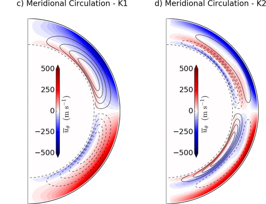
Figure 11: The average meridional flow profiles for different time periods measured by magnetic pattern tracking of MDI/HMI data are shown in the top panel. The red (blue) represents the flow during cycle 23 (24) maximum. The purple line represents cycle minimum during Solar Cycle 23 and 24. The black line represents an average over both cycles. Two possible, idealized meridional circulation patterns are shown in the bottom panel, adapted from Stejko et al (2021) (reproduced by permission): the classical single-cell with a deep return flow (labeled K1) and a double-cell circulation profile with a stronger return flow (labeled K2).

6.4 Active Region Inflows

Inflows towards AR belts are observed by local helioseismic techniques (e.g., (Gizon et al, 2001; Zhao and Kosovichev, 2004; Haber et al, 2004; González Hernández et al, 2008b) and these flows are observed from approximately 10^∘ from the AR with amplitudes up to 50 m s^-1 of horizontal velocities. The AR inflows modulate the N-S meridional flow, which is on the same order of magnitude.

The explanation for the inflows is a geostrophic flow caused by increased radiative loss in the AR belt (Gizon and Rempel, 2008). Gottschling et al (2022) studied the evolution of the AR inflows and reports that converging flows are present one day prior to emergence and that these pre-emergence flows do not depend on latitude or flux. A prograde flow of about 40 m s^-1 is found at the leading polarity during emergence (Birch et al, 2019; Gottschling et al, 2022) with the increase in amplitudes of the inflows occurring between 1$-$4 days after emergence.

One important consequence of AR inflows is that they slow the flux diffusion, advection, and cancellation (De Rosa and Schrijver, 2006). Surface flux transport modeling highlights how AR inflows may modulate the amplitude of the global magnetic field in several ways. First, AR inflows can limit the latitudinal separation of the AR polarities, thus weakening of the contribution of a given bipolar region to the axial dipole field (Jiang et al, 2010), or second, by increasing the cross-equatorial transport of magnetic flux in weaker cycles, when sunspots emerge at lower latitudes, which ultimately strengthens the axial dipole field (Cameron and Schüssler, 2012). For further discussion of the implementation of AR inflows into surface flux transport models, and the results thereof, see Yeates et al (2023) discussion on fluctuating large-scale flows.

7 Short-Term Solar Cycle Variability

There are two significant variations seen in solar-cycle data (i.e., sunspot number and area, 10.7 cm radio emission, mean solar magnetic field, coronal green line, H-alpha flare number, solar neutrino flux, p-mode frequencies) on a time period shorter than the sunspot cycle: the quasi-biennial oscillation (QBO) (1$-$4 years) and Rieger-type variations (50$-$200 days). The QBO was observed as a roughly 2-year period (Benevolenskaya, 1995) in polar field components and also manifests as the double peak in sunspot numbers observed most easily near the maximum of the sunspot cycle. This double-peak is also known as the Gnevyshev gap (Gnevyshev, 1967). A thorough look at QBOs can be found in Bazilevskaya et al (2014) in which the following characteristics are listed: the QBO timescales change within the range 1 – 4 years with no dominant frequency; they develop in each solar hemisphere independently, but are synchronous within one hemisphere with signatures in the atmosphere and beneath the photosphere based on helioseismology (Bazilevskaya et al, 2014); they are observed in the photospheric magnetic field in phase with other solar activity indices; the QBOs are transferred into the interplanetary medium by the Sun’s open magnetic flux. The Rieger type variations were first observed in gamma-ray flare activity in the 1980s with a 154 d periodicity (Rieger et al, 1984). They were subsequently shown to have many shorter periodicities and be present in sunspot number and area and photospheric magnetic field indices (Bai, 2003).

Other stars show secondary, shorter cycles with smaller amplitudes than their primary cycle (Böhm-Vitense, 2007), and one explanation is that the dynamo is fed by the deep-seated and near-surface shear layer. Another explanation is that the QBOs are caused by the interaction between the dipole and quadrupole terms of the solar dynamo(Wang and Sheeley, 2003). The physical mechanisms responsible for the Rieger type variability may be as simple as AR evolution (Vecchio et al, 2012) or a harmonic of the QBO (Krivova and Solanki, 2002). One compelling mechanism that can produce a range of short-term variability is found in MHD shallow-water modeling of an instability involving the differential rotation and toroidal field bands in the solar tachocline (Dikpati and Gilman, 2005). This instability generates quasi-periodic tachocline nonlinear oscillations (TNOs) with periodicities of 2-20 months that can be correlated with the formation of persistent active longitudes (de Toma et al, 2000) seen in photospheric magnetic field data. (Dikpati et al, 2018, 2021). The mechanism involves the production of upward bulges at selected longitudes in the overshoot tachocline that contain significant toroidal fields. For a review of long-term modulation of the solar cycle, see Biswas et al (2023).

8 Helioseismic Mode Parameter Changes

The frequency (e.g. Woodard and Noyes, 1985; Libbrecht and Woodard, 1990; Elsworth et al, 1990), amplitude (e.g. Elsworth et al, 1993), and lifetime(Chaplin et al, 2000; Komm et al, 2002) of the acoustic modes used in helioseismology all vary with the solar cycle, and they are spatially and temporally correlated with magnetic activity on a wide range of scales, with changes in low-degree modes following global activity measures such as the sunspot number and 10.7 cm radio flux (RF), while in local helioseismology we can see changes down to the scale of ARs (Hindman et al, 2000; Rajaguru et al, 2001; Howe et al, 2004). Most of these changes are believed (e.g. Libbrecht and Woodard, 1990)to arise quite close to the surface, where the cavity in which the modes propagate is modified directly or indirectly by the presence of activity and the excitation and damping of the modes influenced by magnetic fields. The exact interpretation of these changes is difficult, but, for example

Basu and Mandel (2004), Verner et al (2006), and more recently Watson and Basu (2020) found evidence of solar-cycle changes in the signature that the helium ionization zone at 0.98 ${\mathrm{R}_{\odot}}$ makes in helioseismic frequencies. These near-surface effects dominate the changes and make it difficult to use helioseismology to infer changes in the internal solar structure or magnetic fields.

While short-lived, high-degree modes can be used to study local, near-surface effects on timescales as short as a day, global helioseismology requires integration times of at least a few solar rotations to obtain the necessary precision to resolve the interior structure and dynamics, and this precludes the possibility, for example, of using helioseismology to follow the rise of an individual flux tube through the convection zone. On the timescale of a solar cycle, some marginal effects have been reported. For example, Baldner and Basu (2008) and more recently Basu (2021) found small changes in the sound speed at the base of the convection zone. The latter work reports a change of about $2\times 10^{-5}$ in the squared sound-speed at the base of the convection zone between solar maximum and minimum, anticorrelated with the activity level; this is just below the $3\times 10^{-5}$ upper limit found by Eff-Darwich et al (2002). Small changes in the sound-speed near the base of the convection zone were also seen by Chou and Serebryanskiy (2005) using a different technique. Because these effects are so difficult to measure, they have not been widely studied. Any effects of solar-cycle changes in the magnetic fields near the base of the convection zone, which could be valuable to help in understanding the solar dynamo, remain close to or below the limits of detection.

9 Discussion

The traditional index of solar activity is the (group) sunspot number, which however, is robustly defined before the middle of the 19th century and particularly poor in the first half of the 18th century. The research community is working hard to reconcile the sunspot dataset.

While the solar-cycle phenomena in the Sun’s surface and outer atmosphere can be studied in great detail using a variety of observing techniques, helioseismology reveals motions – and to a limited extent structural changes related to the solar cycle – far below the photosphere. The torsional oscillation and the meridional circulation penetrate throughout the convection zone and play a crucial role in the solar dynamo. Therefore, it is imperative that we achieve an unambiguous inference of the structure of the meridional circulation at depth and its evolution over the solar cycle. If, for example, the observations completely ruled out a single-cell meridional circulation flow in each hemisphere, it would rule out dynamo models that rely on such a configuration.

We are able to infer flows at depths, yet the great majority of solar magnetic fields remain unobserved in the solar interior. The bipolar magnetic regions observed in the photosphere represent only the “tip of the iceberg”. Until we can reliably infer magnetic field strengths and dynamics in the interior, we must rely on observations at the surface coupled with simulations to infer dynamics, amplitude and structure of the magnetic fields at depth.

To be considered successful, solar dynamo theories and simulations must be able to reproduce, to some degree, key observations. This includes the modulation of cycle amplitude as measured in the sunspot number, the observed large-scale flows, the adherence to Hale’s law, the trends and inherent scatter in the tilt angles, the equator-ward migration of the active latitudes that produces the butterfly diagram, the evolution of the polar fields.

Declarations

Funding I.U. acknowledges partial support from the Academy of Finland (project 321882 ESPERA). L.U. was supported by NASA Heliophysics Living With a Star grants 80HQTR18T0023, 80NSSC20K0220, and 80NSSC23K0048 and NASA grant 80NSSC22M0162 to the COFFIES DRIVE Center managed by Stanford University. A.N. acknowledges NASA DRIVE Center COFFIES grant 80NSSC20K0602. R.H. acknowledges the support of the UK Science and Technology Facilities Council (STFC) through grant ST/V000500/1. Author Contributions I.U. contributed $\mathsection$2 and Figure 1. A.N. contributed $\mathsection$1, 3, 6.4, 7 and Figures 2 and 3. L.U. contributed $\mathsection$4, 5 and Figures 4, 5, 6, 10 and 11. R.H. contributed $\mathsection$6.1-3, 8 and Figures 7, 8, and 9. All authors reviewed the full manuscript and contributed to $\mathsection$9.

Conflicts of Interest The authors have no relevant financial or non-financial conflicts of interest to disclose.

Acknowledgments All authors thank the International Space Science Institute for supporting the workshop where this review originated.

References

- \bibcommenthead
- Antia and Basu (2001) Antia HM, Basu S (2001) Temporal Variations of the Solar Rotation Rate at High Latitudes. ApJ559(1):L67–L70. 10.1086/323701, https://arxiv.org/abs/arXiv:astro-ph/0108226 [astro-ph]
- Asvestari et al (2017) Asvestari E, Usoskin IG, Kovaltsov GA, et al (2017) Assessment of different sunspot number series using the cosmogenic isotope 44Ti in meteorites. Monthly Notes Royal Astro Soc 467:1608–1613. 10.1093/mnras/stx190
- Babcock (1961) Babcock HW (1961) The Topology of the Sun’s Magnetic Field and the 22-YEAR Cycle. ApJ133:572. 10.1086/147060
- Bai (2003) Bai T (2003) Periodicities in Solar Flare Occurrence: Analysis of Cycles 19-23. ApJ591(1):406–415. 10.1086/375295
- Baldner and Basu (2008) Baldner CS, Basu S (2008) Solar Cycle Related Changes at the Base of the Convection Zone. ApJ686(2):1349–1361. 10.1086/591514, https://arxiv.org/abs/arXiv:0807.0442 [astro-ph]
- Basu (2021) Basu S (2021) Evidence of Solar-cycle-related Structural Changes in the Solar Convection Zone. ApJ917(1):45. 10.3847/1538-4357/ac0c11, https://arxiv.org/abs/arXiv:2106.08383 [astro-ph.SR]
- Basu and Mandel (2004) Basu S, Mandel A (2004) Does Solar Structure Vary with Solar Magnetic Activity? ApJ617(2):L155–L158. 10.1086/427435, https://arxiv.org/abs/arXiv:astro-ph/0411427 [astro-ph]
- Bazilevskaya et al (2014) Bazilevskaya G, Broomhall AM, Elsworth Y, et al (2014) A Combined Analysis of the Observational Aspects of the Quasi-biennial Oscillation in Solar Magnetic Activity. Space Sci. Rev.186(1-4):359–386. 10.1007/s11214-014-0068-0
- Beck (2000) Beck JG (2000) A comparison of differential rotation measurements - (Invited Review). Sol. Phys.191(1):47–70. 10.1023/A:1005226402796
- Bekki and Yokoyama (2017) Bekki Y, Yokoyama T (2017) Double-cell-type Solar Meridional Circulation Based on a Mean-field Hydrodynamic Model. ApJ835(1):9. 10.3847/1538-4357/835/1/9, https://arxiv.org/abs/arXiv:1612.00174 [astro-ph.SR]
- Benevolenskaya (1995) Benevolenskaya EE (1995) Double Magnetic Cycle of Solar Activity. Sol. Phys.161(1):1–8. 10.1007/BF00732080
- Bhowmik et al (2023) Bhowmik P, Jiang J, Upton L, et al (2023) Physical Models for Solar Cycle Predictions. Space Sci. Rev.219(5):40. 10.1007/s11214-023-00983-x, https://arxiv.org/abs/arXiv:2303.12648 [astro-ph.SR]
- Birch et al (2019) Birch AC, Schunker H, Braun DC, et al (2019) Average surface flows before the formation of solar active regions and their relationship to the supergranulation pattern. A&A628:A37. 10.1051/0004-6361/201935591
- Biswas et al (2023) Biswas A, Karak BB, Usoskin I, et al (2023) Long-Term Modulation of Solar Cycles. Space Sci. Rev.219(3):19. 10.1007/s11214-023-00968-w, https://arxiv.org/abs/arXiv:2302.14845 [astro-ph.SR]
- Böhm-Vitense (2007) Böhm-Vitense E (2007) Chromospheric Activity in G and K Main-Sequence Stars, and What It Tells Us about Stellar Dynamos. ApJ657(1):486–493. 10.1086/510482
- Cameron and Schüssler (2023) Cameron R, Schüssler M (2023) Observationally guided models for the solar dynamo and the role of the surface field. arXiv e-prints arXiv:2305.02253. 10.48550/arXiv.2305.02253, https://arxiv.org/abs/arXiv:2305.02253 [astro-ph.SR]
- Cameron and Schüssler (2012) Cameron RH, Schüssler M (2012) Are the strengths of solar cycles determined by converging flows towards the activity belts? A&A548:A57. 10.1051/0004-6361/201219914, https://arxiv.org/abs/arXiv:1210.7644 [astro-ph.SR]
- Cameron et al (2018) Cameron RH, Duvall TL, Schüssler M, et al (2018) Observing and modeling the poloidal and toroidal fields of the solar dynamo. A&A609:A56. 10.1051/0004-6361/201731481, https://arxiv.org/abs/arXiv:1710.07126 [astro-ph.SR]
- Carrasco et al (2021) Carrasco VMS, Hayakawa H, Kuroyanagi C, et al (2021) Strong evidence of low levels of solar activity during the Maunder Minimum. Mon Not R Astron Soc 504(4):5199–5204. 10.1093/mnras/stab1155
- Chaplin et al (2000) Chaplin WJ, Elsworth Y, Isaak GR, et al (2000) Variations in the excitation and damping of low-l solar p modes over the solar activity cycle∗. MNRAS313(1):32–42. 10.1046/j.1365-8711.2000.03176.x
- Charbonneau and Sokoloff (2023) Charbonneau P, Sokoloff D (2023) Evolution of Solar and Stellar Dynamo Theory. Space Sci. Rev.219(5):35. 10.1007/s11214-023-00980-0, https://arxiv.org/abs/arXiv:2305.16553 [astro-ph.SR]
- Charbonneau et al (2005) Charbonneau P, St-Jean C, Zacharias P (2005) Fluctuations in Babcock-Leighton Dynamos. I. Period Doubling and Transition to Chaos. ApJ619(1):613–622. 10.1086/426385
- Chatzistergos et al (2017) Chatzistergos T, Usoskin IG, Kovaltsov GA, et al (2017) New reconstruction of the sunspot group numbers since 1739 using direct calibration and “backbone” methods. Astron Astrophys 602:A69. 10.1051/0004-6361/201630045, https://arxiv.org/abs/arXiv:1702.06183 [astro-ph.SR]
- Chou and Serebryanskiy (2005) Chou DY, Serebryanskiy A (2005) In Search of the Solar Cycle Variations of p-Mode Frequencies Generated by Perturbations in the Solar Interior. ApJ624:420–427. 10.1086/428925, https://arxiv.org/abs/astro-ph/0405175
- Clette and Lefèvre (2016) Clette F, Lefèvre L (2016) The New Sunspot Number: Assembling All Corrections. Solar Phys 291:2629–2651. 10.1007/s11207-016-1014-y
- Clette et al (2007) Clette F, Berghmans D, Vanlommel P, et al (2007) From the Wolf number to the International Sunspot Index: 25 years of SIDC. Adv Space Res 40:919–928. 10.1016/j.asr.2006.12.045
- Clette et al (2014) Clette F, Svalgaard L, Vaquero J, et al (2014) Revisiting the sunspot number: A 400-year perspective on the solar cycle. Space Sci Rev 186:35. 10.1007/s11214-014-0074-2
- Corbard et al (1999) Corbard T, Blanc-Féraud L, Berthomieu G, et al (1999) Non linear regularization for helioseismic inversions. Application for the study of the solar tachocline. A&A344:696–708. https://arxiv.org/abs/arXiv:astro-ph/9901112 [astro-ph]
- Couvidat et al (2003) Couvidat S, García RA, Turck-Chièze S, et al (2003) The Rotation of the Deep Solar Layers. ApJ597(1):L77–L79. 10.1086/379698, https://arxiv.org/abs/arXiv:astro-ph/0309806 [astro-ph]
- Dasi-Espuig et al (2010) Dasi-Espuig M, Solanki SK, Krivova NA, et al (2010) Sunspot group tilt angles and the strength of the solar cycle. A&A518:A7. 10.1051/0004-6361/201014301, https://arxiv.org/abs/arXiv:1005.1774 [astro-ph.SR]
- De Rosa and Schrijver (2006) De Rosa ML, Schrijver CJ (2006) Consequences of large-scale flows around active regions on the dispersal of magnetic field across the solar surface. In: Fletcher K, Thompson M (eds) Proceedings of SOHO 18/GONG 2006/HELAS I, Beyond the spherical Sun, p 12
- de Toma et al (2000) de Toma G, White OR, Harvey KL (2000) A Picture of Solar Minimum and the Onset of Solar Cycle 23. I. Global Magnetic Field Evolution. ApJ529(2):1101–1114. 10.1086/308299
- Dikpati and Charbonneau (1999a) Dikpati M, Charbonneau P (1999a) A Babcock-Leighton Flux Transport Dynamo with Solar-like Differential Rotation. ApJ518(1):508–520. 10.1086/307269
- Dikpati and Charbonneau (1999b) Dikpati M, Charbonneau P (1999b) Intermittency in Solar Cycle Caused by Stochastic Fluctuation in Meridional Circulation. In: American Astronomical Society Meeting Abstracts #194, p 92.04
- Dikpati and Gilman (2005) Dikpati M, Gilman PA (2005) A Shallow-Water Theory for the Sun’s Active Longitudes. ApJ635(2):L193–L196. 10.1086/499626
- Dikpati et al (2018) Dikpati M, McIntosh SW, Bothun G, et al (2018) Role of Interaction between Magnetic Rossby Waves and Tachocline Differential Rotation in Producing Solar Seasons. ApJ853(2):144. 10.3847/1538-4357/aaa70d
- Dikpati et al (2021) Dikpati M, McIntosh SW, Chatterjee S, et al (2021) Deciphering the Deep Origin of Active Regions via Analysis of Magnetograms. ApJ910(2):91. 10.3847/1538-4357/abe043
- D’Silva and Choudhuri (1993) D’Silva S, Choudhuri AR (1993) A theoretical model for tilts of bipolar magnetic regions. A&A272:621
- Eddy (1976) Eddy J (1976) The maunder minimum. Science 192:1189–1202. 10.1126/science.192.4245.1189
- Eff-Darwich and Korzennik (1998) Eff-Darwich A, Korzennik SG (1998) The Rotation of the Solar Core: Compatibility of the Different Data Sets Available. In: Korzennik S (ed) Structure and Dynamics of the Interior of the Sun and Sun-like Stars, p 685
- Eff-Darwich et al (2002) Eff-Darwich A, Korzennik SG, Jiménez-Reyes SJ, et al (2002) An Upper Limit on the Temporal Variations of the Solar Interior Stratification. ApJ580(1):574–578. 10.1086/343063, https://arxiv.org/abs/arXiv:astro-ph/0207402 [astro-ph]
- Elsworth et al (1990) Elsworth Y, Howe R, Isaak GR, et al (1990) Variation of low-order acoustic solar oscillations over the solar cycle. Nature345:322–324. 10.1038/345322a0
- Elsworth et al (1993) Elsworth Y, Howe R, Isaak GR, et al (1993) The variation in the strength of low-l solar p-modes - 1981-92. MNRAS265:888–898
- Fan (2009) Fan Y (2009) Magnetic Fields in the Solar Convection Zone. Living Reviews in Solar Physics 6(1):4. 10.12942/lrsp-2009-4
- Fisher et al (1995) Fisher GH, Fan Y, Howard RF (1995) Comparisons between Theory and Observation of Active Region Tilts. ApJ438:463. 10.1086/175090
- Friedli (2020) Friedli TK (2020) Recalculation of the Wolf Series from 1877 to 1893. Solar Phys 295(6):72. 10.1007/s11207-020-01637-9
- Gilman and Howard (1986) Gilman PA, Howard R (1986) Rotation and Expansion within Sunspot Groups. ApJ303:480. 10.1086/164093
- Gilman and Howe (2003) Gilman PA, Howe R (2003) Meridional motion and the slope of isorotation contours. In: Sawaya-Lacoste H (ed) ESA SP-517: GONG+ 2002. Local and Global Helioseismology: the Present and Future, pp 283–285
- Gizon (2004) Gizon L (2004) Helioseismology of Time-Varying Flows Through The Solar Cycle. Sol. Phys.224(1-2):217–228. 10.1007/s11207-005-4983-9
- Gizon and Rempel (2008) Gizon L, Rempel M (2008) Observation and Modeling of the Solar-Cycle Variation of the Meridional Flow. Sol. Phys.251(1-2):241–250. 10.1007/s11207-008-9162-3, https://arxiv.org/abs/arXiv:0803.0950 [astro-ph]
- Gizon et al (2001) Gizon L, Duvall JT. L., Larsen RM (2001) Probing Surface Flows and Magnetic Activity with Time-Distance Helioseismology. In: Brekke P, Fleck B, Gurman JB (eds) Recent Insights into the Physics of the Sun and Heliosphere: Highlights from SOHO and Other Space Missions, p 189
- Gizon et al (2020) Gizon L, Cameron RH, Pourabdian M, et al (2020) Meridional flow in the Sun’s convection zone is a single cell in each hemisphere. Science 368(6498):1469–1472. 10.1126/science.aaz7119
- Gnevyshev (1967) Gnevyshev MN (1967) On the 11-Years Cycle of Solar Activity. Sol. Phys.1(1):107–120. 10.1007/BF00150306
- González Hernández et al (2008a) González Hernández I, Kholikov S, Hill F, et al (2008a) Subsurface Meridional Circulation in the Active Belts. Sol. Phys.252(2):235–245. 10.1007/s11207-008-9264-y, https://arxiv.org/abs/arXiv:0808.3606 [astro-ph]
- González Hernández et al (2008b) González Hernández I, Kholikov S, Hill F, et al (2008b) Subsurface Meridional Circulation in the Active Belts. Sol. Phys.252(2):235–245. 10.1007/s11207-008-9264-y, https://arxiv.org/abs/arXiv:0808.3606 [astro-ph]
- Gottschling et al (2022) Gottschling N, Schunker H, Birch AC, et al (2022) Testing solar surface flux transport models in the first days after active region emergence. A&A660:A6. 10.1051/0004-6361/202142071, https://arxiv.org/abs/arXiv:2111.01896 [astro-ph.SR]
- Haber et al (2004) Haber DA, Hindman BW, Toomre J, et al (2004) Organized Subsurface Flows near Active Regions. Sol. Phys.220(2):371–380. 10.1023/B:SOLA.0000031405.52911.08
- Hagenaar et al (2003) Hagenaar HJ, Schrijver CJ, Title AM (2003) The Properties of Small Magnetic Regions on the Solar Surface and the Implications for the Solar Dynamo(s). ApJ584(2):1107–1119. 10.1086/345792
- Hale (1908) Hale GE (1908) On the Probable Existence of a Magnetic Field in Sun-Spots. ApJ28:315. 10.1086/141602
- Hanasoge (2022) Hanasoge SM (2022) Surface and interior meridional circulation in the Sun. Living Reviews in Solar Physics 19(1):3. 10.1007/s41116-022-00034-7
- Harvey (1994) Harvey KL (1994) The solar magnetic cycle. In: Rutten RJ, Schrijver CJ (eds) Solar Surface Magnetism, p 347
- Harvey-Angle (1993) Harvey-Angle KL (1993) ”magnetic bipoles on the sun”. PhD thesis, -
- Hathaway (2012) Hathaway DH (2012) Supergranules as Probes of the Sun’s Meridional Circulation. ApJ760(1):84. 10.1088/0004-637X/760/1/84, https://arxiv.org/abs/arXiv:1210.3343 [astro-ph.SR]
- Hathaway and Rightmire (2010) Hathaway DH, Rightmire L (2010) Variations in the Sun’s Meridional Flow over a Solar Cycle. Science 327(5971):1350. 10.1126/science.1181990
- Hathaway et al (2022) Hathaway DH, Upton LA, Mahajan SS (2022) Variations in differential rotation and meridional flow within the Sun’s surface shear layer 1996–2022. Frontiers in Astronomy and Space Sciences 9:419. 10.3389/fspas.2022.1007290, https://arxiv.org/abs/arXiv:2212.10619 [astro-ph.SR]
- Hayakawa et al (2021) Hayakawa H, Lockwood M, Owens M, et al (2021) Graphical evidence for the solar coronal structure during the Maunder minimum: comparative study of the total eclipse drawings in 1706 and 1715. J Space Weather Space Climate 11:1. 10.1051/swsc/2020035
- Hazra et al (2023) Hazra G, Nandy D, Kitchatinov L, et al (2023) Mean Field Models of Flux Transport Dynamo and Meridional Circulation in the Sun and Stars. Space Sci. Rev.219(5):39. 10.1007/s11214-023-00982-y, https://arxiv.org/abs/arXiv:2302.09390 [astro-ph.SR]
- Hindman et al (2000) Hindman B, Haber D, Toomre J, et al (2000) Local Fractional Frequency Shifts Used as Tracers of Magnetic Activity. Sol. Phys.192:363–372. 10.1023/A:1005283302728
- Hoeksema (1995) Hoeksema JT (1995) The Large-Scale Structure of the Heliospheric Current Sheet During the ULYSSES Epoch. Space Sci. Rev.72(1-2):137–148. 10.1007/BF00768770
- Hotta et al (2023) Hotta H, Bekki Y, Gizon L, et al (2023) Dynamics of solar large-scale flows. arXiv e-prints arXiv:2307.06481. 10.48550/arXiv.2307.06481, https://arxiv.org/abs/arXiv:2307.06481 [astro-ph.SR]
- Howard and LaBonte (1980) Howard R, LaBonte BJ (1980) The sun is observed to be a torsional oscillator with a period of 11 years. ApJ239:L33–L36. 10.1086/183286
- Howe (2009) Howe R (2009) Solar Interior Rotation and its Variation. Living Reviews in Solar Physics 6(1):1. 10.12942/lrsp-2009-1, https://arxiv.org/abs/arXiv:0902.2406 [astro-ph.SR]
- Howe et al (2000) Howe R, Christensen-Dalsgaard J, Hill F, et al (2000) Deeply Penetrating Banded Zonal Flows in the Solar Convection Zone. ApJ533:L163–L166. 10.1086/312623, https://arxiv.org/abs/astro-ph/0003121
- Howe et al (2004) Howe R, Komm RW, Hill F, et al (2004) Activity-related Changes in Local Solar Acoustic Mode Parameters from Michelson Doppler Imager and Global Oscillations Network Group. ApJ608(1):562–579. 10.1086/392525
- Howe et al (2009) Howe R, Christensen-Dalsgaard J, Hill F, et al (2009) A Note on the Torsional Oscillation at Solar Minimum. ApJ701(2):L87–L90. 10.1088/0004-637X/701/2/L87, https://arxiv.org/abs/arXiv:0907.2965 [astro-ph.SR]
- Howe et al (2013) Howe R, Christensen-Dalsgaard J, Hill F, et al (2013) The High-latitude Branch of the Solar Torsional Oscillation in the Rising Phase of Cycle 24. ApJ767(1):L20. 10.1088/2041-8205/767/1/L20
- Howe et al (2018) Howe R, Hill F, Komm R, et al (2018) Signatures of Solar Cycle 25 in Subsurface Zonal Flows. ApJ862(1):L5. 10.3847/2041-8213/aad1ed, https://arxiv.org/abs/arXiv:1807.02398 [astro-ph.SR]
- Howe et al (2022) Howe R, Chaplin WJ, Christensen-Dalsgaard J, et al (2022) Update on global helioseismic observations of the solar torsional oscillation. Research Notes of the AAS 6(12):261. 10.3847/2515-5172/aca97d, URL https://dx.doi.org/10.3847/2515-5172/aca97d
- Hoyt and Schatten (1998) Hoyt DV, Schatten KH (1998) Group Sunspot Numbers: A New Solar Activity Reconstruction. Solar Phys 181:491–512. 10.1023/A:1005056326158
- Ivanov and Miletsky (2011) Ivanov VG, Miletsky EV (2011) Width of Sunspot Generating Zone and Reconstruction of Butterfly. Sol. Phys.268(1):231–242. 10.1007/s11207-010-9665-6, https://arxiv.org/abs/arXiv:1011.4800 [astro-ph.SR]
- Jiang et al (2009) Jiang J, Cameron R, Schmitt D, et al (2009) Countercell Meridional Flow and Latitudinal Distribution of the Solar Polar Magnetic Field. ApJ693(2):L96–L99. 10.1088/0004-637X/693/2/L96
- Jiang et al (2010) Jiang J, Işik E, Cameron RH, et al (2010) The Effect of Activity-related Meridional Flow Modulation on the Strength of the Solar Polar Magnetic Field. ApJ717(1):597–602. 10.1088/0004-637X/717/1/597, https://arxiv.org/abs/arXiv:1005.5317 [astro-ph.SR]
- Jiang et al (2014) Jiang J, Cameron RH, Schüssler M (2014) Effects of the Scatter in Sunspot Group Tilt Angles on the Large-scale Magnetic Field at the Solar Surface. ApJ791(1):5. 10.1088/0004-637X/791/1/5, https://arxiv.org/abs/arXiv:1406.5564 [astro-ph.SR]
- Komm et al (2002) Komm R, Howe R, Hill F (2002) Localizing Width and Energy of Solar Global p-Modes. ApJ572:663–673. 10.1086/340196
- Komm et al (2018) Komm R, Howe R, Hill F (2018) Subsurface Zonal and Meridional Flow During Cycles 23 and 24. Sol. Phys.293(10):145. 10.1007/s11207-018-1365-7
- Krivova and Solanki (2002) Krivova NA, Solanki SK (2002) The 1.3-year and 156-day periodicities in sunspot data: Wavelet analysis suggests a common origin. A&A394:701–706. 10.1051/0004-6361:20021063
- Larmor (1919) Larmor J (1919) How could a rotating body such as the Sun become magnetic. Rep Brit Assoc Adv Sci 159:160
- Larson and Schou (2018) Larson TP, Schou J (2018) Global-Mode Analysis of Full-Disk Data from the Michelson Doppler Imager and the Helioseismic and Magnetic Imager. Sol. Phys.293(2):29. 10.1007/s11207-017-1201-5
- Leighton (1964) Leighton RB (1964) Transport of Magnetic Fields on the Sun. ApJ140:1547. 10.1086/148058
- Lekshmi et al (2018) Lekshmi B, Nandy D, Antia HM (2018) Asymmetry in Solar Torsional Oscillation and the Sunspot Cycle. ApJ861(2):121. 10.3847/1538-4357/aacbd5, https://arxiv.org/abs/arXiv:1807.03588 [astro-ph.SR]
- Lemerle and Charbonneau (2017) Lemerle A, Charbonneau P (2017) A Coupled 2 × 2D Babcock-Leighton Solar Dynamo Model. II. Reference Dynamo Solutions. ApJ834(2):133. 10.3847/1538-4357/834/2/133, https://arxiv.org/abs/arXiv:1606.07375 [astro-ph.SR]
- Leussu et al (2013) Leussu R, Usoskin IG, Arlt R, et al (2013) Inconsistency of the Wolf sunspot number series around 1848. Astron Astrophys 559:A28. 10.1051/0004-6361/201322373, https://arxiv.org/abs/arXiv:1310.8443 [astro-ph.SR]
- Li (2018) Li J (2018) A Systematic Study of Hale and Anti-Hale Sunspot Physical Parameters. ApJ867(2):89. 10.3847/1538-4357/aae31a, https://arxiv.org/abs/arXiv:1809.08980 [astro-ph.SR]
- Libbrecht and Woodard (1990) Libbrecht KG, Woodard MF (1990) Solar-cycle effects on solar oscillation frequencies. Nature345:779–782. 10.1038/345779a0
- Maunder (1903) Maunder EW (1903) Spoerer’s law of zones. The Observatory 26:329–330
- Maunder (1904) Maunder EW (1904) Note on the Distribution of Sun-spots in Heliographic Latitude, 1874-1902. MNRAS64:747–761. 10.1093/mnras/64.8.747
- McClintock and Norton (2013) McClintock BH, Norton AA (2013) Recovering Joy’s Law as a Function of Solar Cycle, Hemisphere, and Longitude. Sol. Phys.287(1-2):215–227. 10.1007/s11207-013-0338-0, https://arxiv.org/abs/arXiv:1305.3205 [astro-ph.SR]
- McClintock and Norton (2016) McClintock BH, Norton AA (2016) Tilt Angle and Footpoint Separation of Small and Large Bipolar Sunspot Regions Observed with HMI. ApJ818(1):7. 10.3847/0004-637X/818/1/7, https://arxiv.org/abs/arXiv:1602.04154 [astro-ph.SR]
- McClintock et al (2014) McClintock BH, Norton AA, Li J (2014) Re-examining Sunspot Tilt Angle to Include Anti-Hale Statistics. ApJ797(2):130. 10.1088/0004-637X/797/2/130, https://arxiv.org/abs/arXiv:1412.5094 [astro-ph.SR]
- Muñoz-Jaramillo et al (2013) Muñoz-Jaramillo A, Dasi-Espuig M, Balmaceda LA, et al (2013) Solar Cycle Propagation, Memory, and Prediction: Insights from a Century of Magnetic Proxies. ApJ767(2):L25. 10.1088/2041-8205/767/2/L25, https://arxiv.org/abs/arXiv:1304.3151 [astro-ph.SR]
- Muñoz-Jaramillo et al (2021) Muñoz-Jaramillo A, Navarrete B, Campusano LE (2021) Solar Anti-Hale Bipolar Magnetic Regions: A Distinct Population with Systematic Properties. ApJ920(1):31. 10.3847/1538-4357/ac133b, https://arxiv.org/abs/arXiv:2203.11898 [astro-ph.SR]
- Nagy et al (2017) Nagy M, Lemerle A, Labonville F, et al (2017) The Effect of “Rogue” Active Regions on the Solar Cycle. Sol. Phys.292(11):167. 10.1007/s11207-017-1194-0, https://arxiv.org/abs/arXiv:1712.02185 [astro-ph.SR]
- Nagy et al (2020) Nagy M, Lemerle A, Charbonneau P (2020) Impact of nonlinear surface inflows into activity belts on the solar dynamo. Journal of Space Weather and Space Climate 10:62. 10.1051/swsc/2020064
- Nelson et al (2013) Nelson NJ, Brown BP, Brun AS, et al (2013) Magnetic Wreaths and Cycles in Convective Dynamos. ApJ762(2):73. 10.1088/0004-637X/762/2/73, https://arxiv.org/abs/arXiv:1211.3129 [astro-ph.SR]
- Norton and Gilman (2005) Norton AA, Gilman PA (2005) Recovering Solar Toroidal Field Dynamics from Sunspot Location Patterns. ApJ630(2):1194–1205. 10.1086/431961, https://arxiv.org/abs/arXiv:astro-ph/0506025 [astro-ph]
- Norton et al (2014) Norton AA, Charbonneau P, Passos D (2014) Hemispheric Coupling: Comparing Dynamo Simulations and Observations. Space Sci. Rev.186(1-4):251–283. 10.1007/s11214-014-0100-4, https://arxiv.org/abs/arXiv:1411.7052 [astro-ph.SR]
- Norton et al (2017) Norton AA, Jones EH, Linton MG, et al (2017) Magnetic Flux Emergence and Decay Rates for Preceder and Follower Sunspots Observed with HMI. ApJ842(1):3. 10.3847/1538-4357/aa7052, https://arxiv.org/abs/arXiv:1705.02053 [astro-ph.SR]
- Petrovay (2010) Petrovay K (2010) Solar Cycle Prediction. Living Reviews in Solar Physics 7:6. 10.12942/lrsp-2010-6, https://arxiv.org/abs/arXiv:1012.5513 [astro-ph.SR]
- Petrovay et al (2020) Petrovay K, Nagy M, Yeates AR (2020) Towards an algebraic method of solar cycle prediction. I. Calculating the ultimate dipole contributions of individual active regions. Journal of Space Weather and Space Climate 10:50. 10.1051/swsc/2020050, https://arxiv.org/abs/arXiv:2009.02299 [astro-ph.SR]
- Rajaguru et al (2001) Rajaguru SP, Basu S, Antia HM (2001) Ring Diagram Analysis of the Characteristics of Solar Oscillation Modes in Active Regions. ApJ563:410–418. 10.1086/323780, https://arxiv.org/abs/astro-ph/0108227
- Rempel (2012) Rempel M (2012) High latitude Solar Torsional Oscillations during Phases of Changing Magnetic Cycle Amplitude. ApJ750(1):L8. 10.1088/2041-8205/750/1/L8
- Rieger et al (1984) Rieger E, Share GH, Forrest DJ, et al (1984) A 154-day periodicity in the occurrence of hard solar flares? Nature312(5995):623–625. 10.1038/312623a0
- Rightmire-Upton et al (2012) Rightmire-Upton L, Hathaway DH, Kosak K (2012) Measurements of the Sun’s High-latitude Meridional Circulation. ApJ761(1):L14. 10.1088/2041-8205/761/1/L14, https://arxiv.org/abs/arXiv:1211.0944 [astro-ph.SR]
- Schatten et al (1978) Schatten KH, Scherrer PH, Svalgaard L, et al (1978) Using Dynamo Theory to predict the sunspot number during Solar Cycle 21. Geophys. Res. Lett.5(5):411–414. 10.1029/GL005i005p00411
- Schou (1999) Schou J (1999) Migration of Zonal Flows Detected Using Michelson Doppler Imager F-Mode Frequency Splittings. ApJ523:L181–L184. 10.1086/312279
- Schou et al (1998) Schou J, Antia HM, Basu S, et al (1998) Helioseismic Studies of Differential Rotation in the Solar Envelope by the Solar Oscillations Investigation Using the Michelson Doppler Imager. ApJ505(1):390–417. 10.1086/306146
- Schunker et al (2020) Schunker H, Baumgartner C, Birch AC, et al (2020) Average motion of emerging solar active region polarities. II. Joy’s law. A&A640:A116. 10.1051/0004-6361/201937322, https://arxiv.org/abs/arXiv:2006.05565 [astro-ph.SR]
- Schwabe (1844) Schwabe H (1844) Sonnenbeobachtungen im Jahre 1843. Von Herrn Hofrath Schwabe in Dessau. Astronomische Nachrichten 21(15):233. 10.1002/asna.18440211505
- Snodgrass and Ulrich (1990) Snodgrass HB, Ulrich RK (1990) Rotation of Doppler Features in the Solar Photosphere. ApJ351:309. 10.1086/168467
- Sporer (1894) Sporer G (1894) Number 32. Zehnten Bandes Erstes Stuck. Beobachtungen von Sonnenflecken in den Jahren 1885 bis 1893. Publikationen des Astrophysikalischen Observatoriums zu Potsdam 10:3–147
- Stejko et al (2021) Stejko AM, Kosovichev AG, Pipin VV (2021) Forward Modeling Helioseismic Signatures of One- and Two-cell Meridional Circulation. ApJ911(2):90. 10.3847/1538-4357/abec70, https://arxiv.org/abs/arXiv:2101.01220 [astro-ph.SR]
- Stenflo (1970) Stenflo JO (1970) Hale’s Attempts to Determine the Sun’s General Magnetic Field. Sol. Phys.14(2):263–273. 10.1007/BF00221312
- Stenflo and Kosovichev (2012) Stenflo JO, Kosovichev AG (2012) Bipolar Magnetic Regions on the Sun: Global Analysis of the SOHO/MDI Data Set. ApJ745(2):129. 10.1088/0004-637X/745/2/129, https://arxiv.org/abs/arXiv:1112.5226 [astro-ph.SR]
- Sun et al (2015) Sun X, Hoeksema JT, Liu Y, et al (2015) On Polar Magnetic Field Reversal and Surface Flux Transport During Solar Cycle 24. ApJ798(2):114. 10.1088/0004-637X/798/2/114, https://arxiv.org/abs/arXiv:1410.8867 [astro-ph.SR]
- Svalgaard and Schatten (2016) Svalgaard L, Schatten KH (2016) Reconstruction of the Sunspot Group Number: The Backbone Method. Solar Phys 291:2653–2684. 10.1007/s11207-015-0815-8, https://arxiv.org/abs/arXiv:1506.00755 [astro-ph.SR]
- Svalgaard et al (1978) Svalgaard L, Duvall JT. L., Scherrer PH (1978) The strength of the Sun’s polar fields. Sol. Phys.58(2):225–239. 10.1007/BF00157268
- Svalgaard et al (2005) Svalgaard L, Cliver EW, Kamide Y (2005) Sunspot cycle 24: Smallest cycle in 100 years? Geophys. Res. Lett.32(1):L01104. 10.1029/2004GL021664
- Thompson et al (1996) Thompson MJ, Toomre J, Anderson ER, et al (1996) Differential Rotation and Dynamics of the Solar Interior. Science 272(5266):1300–1305. 10.1126/science.272.5266.1300
- Tlatov et al (2013) Tlatov A, Illarionov E, Sokoloff D, et al (2013) A new dynamo pattern revealed by the tilt angle of bipolar sunspot groups. MNRAS432(4):2975–2984. 10.1093/mnras/stt659, https://arxiv.org/abs/arXiv:1302.2715 [astro-ph.SR]
- Tlatova et al (2018) Tlatova K, Tlatov A, Pevtsov A, et al (2018) Tilt of Sunspot Bipoles in Solar Cycles 15 to 24. Sol. Phys.293(8):118. 10.1007/s11207-018-1337-y, https://arxiv.org/abs/arXiv:1807.07913 [astro-ph.SR]
- Ulrich (2010) Ulrich RK (2010) Solar meridional circulation from doppler shifts of the fe i line at 5250 a as measured by the 150-foot solar tower telescope at the mt. wilson observatory. The Astrophysical Journal 725(1):658. 10.1088/0004-637X/725/1/658, URL https://dx.doi.org/10.1088/0004-637X/725/1/658
- Ulrich et al (2022) Ulrich RK, Tran T, Boyden JE (2022) Polar upwelling at three sunspot minima. Research Notes of the AAS 6(9):181. 10.3847/2515-5172/ac905f, URL https://doi.org/10.3847/2515-5172/ac905f
- Upton and Hathaway (2014a) Upton L, Hathaway DH (2014a) Effects of Meridional Flow Variations on Solar Cycles 23 and 24. ApJ792(2):142. 10.1088/0004-637X/792/2/142, https://arxiv.org/abs/arXiv:1408.0035 [astro-ph.SR]
- Upton and Hathaway (2014b) Upton LA, Hathaway DH (2014b) Predicting the Sun’s Polar Magnetic Fields with a Surface Flux Transport Model. ApJ780:5. 10.1088/0004-637X/780/1/5, https://arxiv.org/abs/arXiv:1311.0844 [astro-ph.SR]
- Usoskin (2023) Usoskin IG (2023) A History of Solar Activity over Millennia. Living Rev Solar Phys 20:2. 10.1007/s41116-023-00036-z
- Usoskin et al (2015) Usoskin IG, Arlt R, Asvestari E, et al (2015) The Maunder minimum (1645-1715) was indeed a grand minimum: A reassessment of multiple datasets. Astron Astrophys 581:A95. 10.1051/0004-6361/201526652, https://arxiv.org/abs/arXiv:1507.05191 [astro-ph.SR]
- Usoskin et al (2016) Usoskin IG, Kovaltsov GA, Lockwood M, et al (2016) A New Calibrated Sunspot Group Series Since 1749: Statistics of Active Day Fractions. Solar Phys 291:2685–2708. 10.1007/s11207-015-0838-1, https://arxiv.org/abs/arXiv:1512.06421 [astro-ph.SR]
- van Driel-Gesztelyi and Green (2015) van Driel-Gesztelyi L, Green LM (2015) Evolution of Active Regions. Living Reviews in Solar Physics 12(1):1. 10.1007/lrsp-2015-1
- Vaquero et al (2016) Vaquero J, Svalgaard L, Carrasco V, et al (2016) A Revised Collection of Sunspot Group Numbers. Solar Phys 291:3061–3074. 10.1007/s11207-016-0982-2
- Vecchio et al (2012) Vecchio A, Laurenza M, Meduri D, et al (2012) The Dynamics of the Solar Magnetic Field: Polarity Reversals, Butterfly Diagram, and Quasi-biennial Oscillations. ApJ749(1):27. 10.1088/0004-637X/749/1/27
- Verner et al (2006) Verner GA, Chaplin WJ, Elsworth Y (2006) BiSON Data Show Change in Solar Structure with Magnetic Activity. ApJ640(1):L95–L98. 10.1086/503101
- Vorontsov et al (2002) Vorontsov S, Christensen-Dalsgaard J, Schou J, et al (2002) Helioseismic measurement of solar torsional oscillations. Science 296:101–103. 10.1126/science.1069190
- Waldmeier (1961) Waldmeier M (1961) The Sunspot Activity in the Years 1610-1960. Zurich Schulthess and Company AG, Zürich
- Wang and Sheeley (1989) Wang YM, Sheeley JN. R. (1989) Average Properties of Bipolar Magnetic Regions during Sunspot CYCLE-21. Sol. Phys.124(1):81–100. 10.1007/BF00146521
- Wang and Sheeley (1991) Wang YM, Sheeley JN. R. (1991) Magnetic Flux Transport and the Sun’s Dipole Moment: New Twists to the Babcock-Leighton Model. ApJ375:761. 10.1086/170240
- Wang and Sheeley (2003) Wang YM, Sheeley JN. R. (2003) On the Fluctuating Component of the Sun’s Large-Scale Magnetic Field. ApJ590(2):1111–1120. 10.1086/375026
- Wang et al (2015) Wang YM, Colaninno RC, Baranyi T, et al (2015) Active-region Tilt Angles: Magnetic versus White-light Determinations of Joy’s Law. ApJ798(1):50. 10.1088/0004-637X/798/1/50, https://arxiv.org/abs/arXiv:1412.2329 [astro-ph.SR]
- Watson and Basu (2020) Watson CB, Basu S (2020) Solar-cycle-related Changes in the Helium Ionization Zones of the Sun. ApJ903(2):L29. 10.3847/2041-8213/abc348, https://arxiv.org/abs/arXiv:2010.11215 [astro-ph.SR]
- Weber et al (2011) Weber MA, Fan Y, Miesch MS (2011) The Rise of Active Region Flux Tubes in the Turbulent Solar Convective Envelope. ApJ741(1):11. 10.1088/0004-637X/741/1/11, https://arxiv.org/abs/arXiv:1109.0240 [astro-ph.SR]
- Weber et al (2023) Weber MA, Schunker H, Jouve L, et al (2023) Understanding Active Region Emergence and Origins on the Sun and Other Cool Stars. arXiv e-prints arXiv:2306.06536. 10.48550/arXiv.2306.06536, https://arxiv.org/abs/arXiv:2306.06536 [astro-ph.SR]
- Willamo et al (2017) Willamo T, Usoskin IG, Kovaltsov GA (2017) Updated sunspot group number reconstruction for 1749-1996 using the active day fraction method. Astron Astrophys 601:A109. 10.1051/0004-6361/201629839, https://arxiv.org/abs/arXiv:1705.05109 [astro-ph.SR]
- Woodard and Noyes (1985) Woodard MF, Noyes RW (1985) Change of solar oscillation eigenfrequencies with the solar cycle. Nature318(6045):449–450. 10.1038/318449a0
- Yeates et al (2023) Yeates AR, Cheung MCM, Jiang J, et al (2023) Surface Flux Transport on the Sun. arXiv e-prints arXiv:2303.01209. 10.48550/arXiv.2303.01209, https://arxiv.org/abs/arXiv:2303.01209 [astro-ph.SR]
- Zhao and Kosovichev (2004) Zhao J, Kosovichev AG (2004) Torsional Oscillation, Meridional Flows, and Vorticity Inferred in the Upper Convection Zone of the Sun by Time-Distance Helioseismology. ApJ603(2):776–784. 10.1086/381489
- Zhao et al (2013) Zhao J, Bogart RS, Kosovichev AG, et al (2013) Detection of Equatorward Meridional Flow and Evidence of Double-cell Meridional Circulation inside the Sun. ApJ774(2):L29. 10.1088/2041-8205/774/2/L29, https://arxiv.org/abs/arXiv:1307.8422 [astro-ph.SR]
- Zirin (1988) Zirin H (1988) Astrophysics of the sun. ”Cambridge University Press”
- Zolotova and Ponyavin (2015) Zolotova NV, Ponyavin DI (2015) The Maunder Minimum is Not as Grand as it Seemed to be. Astrophys J 800:42. 10.1088/0004-637X/800/1/42