Dictionary Learning under Symmetries via Group Representations

Abstract

The dictionary learning problem can be viewed as a data-driven process to learn a suitable transformation so that data is sparsely represented directly from example data. In this paper, we examine the problem of learning a dictionary that is invariant under a pre-specified group of transformations. Natural settings include Cryo-EM, multi-object tracking, synchronization, pose estimation, etc. We specifically study this problem under the lens of mathematical representation theory. Leveraging the power of non-abelian Fourier analysis for functions over compact groups, we prescribe an algorithmic recipe for learning dictionaries that obey such invariances. We relate the dictionary learning problem in the physical domain, which is naturally modelled as being infinite dimensional, with the associated computational problem, which is necessarily finite dimensional. We establish that the dictionary learning problem can be effectively understood as an optimization instance over certain matrix orbitopes having a particular block-diagonal structure governed by the irreducible representations of the group of symmetries. This perspective enables us to introduce a band-limiting procedure which obtains dimensionality reduction in applications. We provide guarantees for our computational ansatz to provide a desirable dictionary learning outcome. We apply our paradigm to investigate the dictionary learning problem for the groups SO(2) and SO(3). While the SO(2)-orbitope admits an exact spectrahedral description, substantially less is understood about the SO(3)-orbitope. We describe a tractable spectrahedral outer approximation of the SO(3)-orbitope, and contribute an alternating minimization paradigm to perform optimization in this setting. We provide numerical experiments to highlight the efficacy of our approach in learning SO(3)-invariant dictionaries, both on synthetic and on real world data.

Keywords: Group invariance, equivariance, convolutional dictionary learning, Peter-Weyl theorem, non-abelian harmonic analysis, non-commutative Fourier cofficients, band-limited functions, atomic norms, Carathéodory orbitope, semidefinite programming, tensor nuclear norm, alternating projections.

1 Introduction

The ability to model data as sparse vectors under suitable transformations is an essential component of numerous approaches for performing data processing tasks in a range of applications [11, 15]. Prominent examples of such tasks include signal denoising, imputing missing entries in data (such as in low rank matrix or tensor completion), and solving ill-posed inverse problems [6, 7, 13, 14]. At its algorithmic core, these techniques rely on recovering a sparse solution given partial measurements.

1.1 Dictionary Learning

Because of the important role that sparsity plays in these approaches, the success of these methods effectively rely on having access to a suitable transformation so that the data of interest is well-modelled as sparse vectors. The traditional perspective to identifying such transformations is via deep domain expertise – for instance, the use of the discrete cosine transform and wavelets in image processing follows a long lineage of prior works. In recent decades, we have witnessed the emergence of an alternative approach in which we learn the appropriate transformation directly from example data [34, 35]. In the process of doing so, we are now able to readily apply previously developed techniques for data processing applications using these learned transformations – this is especially useful in application domains where a suitable transformation is not a priori available [16, 34, 35].

The process of learning a suitable transform is referred to as the dictionary learning problem in the literature. Mathematically, given a collection of vectors $\{y^{(i)}\}_{i=1}^{n}\subset\mathbb{R}^{d}$, we seek a small collection of vectors $\{\phi_{j}\}_{j=1}^{q}\subset\mathbb{R}^{d}$ so that every data well-approximated by a linear sum of a few of these $\phi$’s

$$y^{(i)}\approx\sum_{j=1}^{q}x_{j}^{(i)}\phi_{j},\qquad\text{ where }\qquad x_{j}^{(i)}\in\mathbb{R},~{}x^{(i)}=(x_{1}^{(i)},\ldots,x_{q}^{(i)})^{T}\text{ is sparse}.$$ (1)

The learned $\phi$’s are often referred to as dictionary atoms. A more compact way to express 1 is as follows

$$y^{(i)}\approx\Phi x^{(i)}\quad\text{ where }\quad x^{(i)}\text{ is sparse},\text{ and }\quad\Phi=[\phi_{1}|\ldots|\phi_{q}].$$

The computational task of obtaining the dictionary atoms $\{\phi_{j}\}$ is typically formulated as a joint optimization instance over the atoms and the coefficients $x^{(i)}$. One such formulation is to incorporate the L1-norm to encourage sparsity in the solution $x^{(i)}$

$$\underset{\Phi,x^{(i)}}{\arg\min}~{}~{}\frac{1}{n}\sum_{i=1}^{n}\left(\|y^{(i)}-\Phi x^{(i)}\|_{2}^{2}+\lambda\|x^{(i)}\|_{1}\right)\quad\text{ s.t. }\quad\|\phi_{j}\|_{2}^{2}=1.$$ (2)

Here, $\lambda\geq 0$ is a regularization parameter. While the optimization instance is not convex, the sub-problem corresponding to fixing one set of variables (either the $\phi$’s or the $x$’s) and optimizing over the other is a convex program .

1.2 Convolutional Dictionary Learning

In certain application domains where dictionary learning techniques are applied, it is sometimes more helpful to permit suitably shifted or transformed copies of a dictionary element as alternative dictionary elements

$$(a_{1},a_{2},\ldots,a_{d})\quad\mapsto\quad(a_{2},a_{3},\ldots,a_{d},a_{1}).$$

The Convolutional Dictionary Learning (abbrv. CDL) problem concerns learning dictionaries with the property that all cyclic shifts (in the coordinates) of a dictionary atom also appear as dictionary atoms. Invariance of the collection of dictionary atoms under shift transformations is a natural modeling assumption in audio processing (in which we perform shifts in the temporal direction) and in image processing (in which shifts occur in the spatial domain) – a substantial body of work devoted to developing computational techniques [20, 25, 48, 49] and applying these to audio processing tasks [5, 23, 29, 38], image processing tasks [30, 36], and time-series analysis [41, 45] have since followed.

The CDL computational task can be phrased, for instance, in terms of the following minimization instance

$$\underset{\Phi,x^{(i)}}{\arg\min}~{}~{}\frac{1}{n}\sum_{i=1}^{n}\left(\|y^{(i)}-\sum_{j=1}^{q}\phi_{j}\ast x^{(i)}\|_{2}^{2}+\lambda\|x^{(i)}\|_{1}\right)\quad\text{ s.t. }\quad\|\phi_{j}\|_{2}^{2}=1,$$ (3)

where $\ast$ denotes convolution, as per usual convention.

If we are to express the problem explicitly in the dictionary atoms, then the formulation would be exactly as in 2, with the modification whereby $\Phi$ has the following structure

$$\Phi=\left[\begin{array}[]{c|c|c|c|c}\Phi_{0}&T\,\Phi_{0}&T^{2}\,\Phi_{0}&\ldots&T^{d-1}\,\Phi_{0}\end{array}\right]\quad\text{ where }\quad\Phi_{0}=\left[\begin{array}[]{c|c|c}\phi_{1}&\ldots&\phi_{q}\end{array}\right].$$ (4)

Here, $T^{k}$ denotes a shift operation by $k$ coordinates.

1.3 Group Invariant Dictionary Learning

This raises the natural question: how do we handle more general symmetries beyond shifts? Applications where there is an action of a natural group of symmetries are many. Prominent examples include natural image data under rotations and translations [27, 26]; data arising in tomography [47, 31]; network based data [22, 24]; synchronization problems in robotics [40]; computer vision [1]; multi-reference alignment (MRA) [2, 37, 18, 21] and cryo electron microscopy (cryo EM) under the action of rigid motions [43, 3].

If the underlying group of transformations is finite then the solution is immediate – we simply append our dictionary with all transformed copies of the atoms as we did in CDL. However, this approach is impractical for large groups. Moreover, if the symmetry is continuous, then such a strategy would not work, even at a conceptual level.

To overcome difficulties arising from working with continuous symmetries, Soh [44] proposed a different alternating minimization framework for learning dictionaries that are invariant to some specified group invariance. Concretely, this task, which we term as the group invariant dictionary learning (abbrv. GIDL) problem, can be described as learning a collection of atoms $\mathcal{K}:=\{\phi_{j}\}_{j=1}^{q}$ satisfying the following :

$$y^{(i)}\approx\sum_{k\in\mathcal{K}}x_{k}^{(i)}\,g_{k}^{(i)}\cdot\phi_{k},\qquad x_{k}^{(i)}\in\mathbb{R},g_{k}^{(i)}\in G,\phi_{k}\in\{\phi_{j}\}_{j=1}^{q},\qquad 1\leq i\leq n.$$ (5)

The elements $g\in G$ model the symmetry transformation. In addition, we impose the additional constraint that the cardinality of the index set should be small relative to the data dimension, i.e. $|\mathcal{K}|=q\ll d$ so as to capture model sparsity.

Suppose, for now, that the symmetry $g$ can be expressed as the action of a linear transformation $\rho(g)$ acting on a vector space $V$

$$g\cdot\phi=\rho(g)\phi\quad\text{ for all }\quad g\in G,\phi\in V.$$

The key contribution in [44] is to formulate the GIDL problem as the solution of the following optimization instance

$$\underset{L_{j}^{(i)},\phi_{j}}{\arg\min}~{}~{}\sum_{i}\big{(}\frac{1}{2}\|y^{(i)}-\sum_{j=1}^{q}L^{(i)}_{j}\phi_{j}\|_{2}^{2}+\lambda\cdot\sum_{j=1}^{q}\|L^{(i)}_{j}\|_{G}\big{)}\qquad\text{s.t.}\qquad\|\phi_{j}\|_{2}^{2}=1,$$ (6)

where the optimization variables $L_{j}^{(i)}$ are operators residing in the space $\mathrm{Span}(\{\rho(g):g\in G\})$. Here, $\|\cdot\|_{G}$ is a convex penalty function – specifically, it is the Minkowski functional induced by the convex hull of the $\rho$’s [4, 10]

$$\|L\|_{G}:=\inf\{~{}t:L\in t\cdot\mathrm{conv}(\{\pm\rho(g):g\in G\})~{}\}.$$

In particular, the $\|\cdot\|_{G}$ has the effect of promoting solutions $L^{(i)}_{j}$ that are sparse linear sums of elements from the set $\{\rho(g):g\in G\}$.

The conceptual difference 6 makes from 3 and 4 is that it lifts the optimization problem from the vector space where the data resides to the vector space where the $\rho$’s representing the transformation reside. In doing so, the problem of representing a data vector $y\in\mathbb{R}^{d}$ sparsely with respect to a group invariant dictionary – even if it is infinite or continuous – can be resolved by solving a finite dimensional convex program; specifically by minimizing with respect to the penalty function $\|\cdot\|_{G}$.

1.4 Our contributions

The framework laid out by Soh in [44] fundamentally relies on two basic ingredients being satisfied for its success

1. We have an explicit description of $\rho$; and

2. We are able to express the convex hull of $\{\rho(g):g\in G\}$ tractably.

In what follows, we lay out our four main contributions in this paper in the above context.

Our first contribution in this work is to address requirement 1. Specifically, in the case where the invariances can be described via the action of a compact group $G$, we describe a systematic recipe for expressing the transformation by a certain explicit action of linear operators. We present key features of this programme below; for details we refer the reader to Sections 2 and 3. The basic idea is to first represent the data as functions over the group $G$, for which we outline a canonical recipe. Second, a fundamental result in the representation theory of compact groups, namely the Peter-Weyl Theorem, entails that every such function admits a generalized Fourier series – unlike the regular Fourier series over periodic functions we are familiar with, the Fourier coefficients may be matrix-valued (as we shall see later, this happens if the group is non-commutative). Third, the Peter Weyl theory also entails that the group action (namely, the regular representation) can be expressed as an operator with the same block diagonal structure as the Fourier series. That is to say, the group action decomposes to a sequence of square blocks, and each block only acts on a single matrix-valued Fourier coefficient, via an explicit matrix multiplication operation.

An important objective of this paper is to spell out the consequences of group representation theory in our dictionary learning problem in a language that is readily accessible to practitioners. On the computational front, there are still a number of issues to resolve. For continuous groups $G$, the functions and operators both reside in infinite dimensional spaces – what then is the appropriate finite dimensional approximation of the dictionary learning problem? Our second contribution is to address these problems.

In this vein, we explore in greater depth the harmonic analytical aspects of our dictionary learning problem. In particular, by drawing the connections of representation theory to our group invariant dictionary learning problem, we are now in a position to pose the following question:

The dictionary learning problem we solve is a computational problem that resides over a finite dimensional space. In reality, the problem we solve is simply a model of a similar task that resides in the physical domain, which is continuous. Is there a principled way of describing what the dictionary learning problem is in the continuous limit? In particular, are we able to also quantify the error between the dictionary elements we learned by solving the finite dimensional approximation from the analogous problem in the continuous limit?

Our third contribution focuses on the harmonic analytical aspects of our dictionary learning problem. Under suitable qualifications, we show that the dictionary elements learned in the finite dimensional approximation converges to the solution of the actual problem in the limit, as the dimensionality increases.

Our fourth contribution is to spell out in detail the above programme for concrete examples of certain groups that are of key importance in applications. On this note, we first discuss the process for SO(2), and how this problem can in fact be viewed as the continuous limit of the CDL problem. Second, we discuss the agenda for SO(3). This is substantially more difficult as it is unknown whether the convex hull of the dictionary elements admits a tractable description. The apparent connection to the tensor nuclear norm ball suggests that this set is probably not tractable to describe. Nevertheless, one can easily write down a simple convex relaxation, and our numerics suggest that the relaxation is actually quite tight.

2 Preliminaries

In this section, we introduce the necessary concepts from group representation theory, harmonic analysis and convex geometry. In particular, we lay out the groundwork for analysing a non-abelian Fourier series expansion for functions over compact groups in the context of the GIDL problem. It is on these non-abelian, matrix-valued Fourier coefficients that our principal dictionary learning algorithms operate.

2.1 Preliminaries on Group Theory

Let $G$ be a multiplicative group whose identity element is denoted as $e$; that is, $aa^{-1}=a^{-1}a=e$ $\forall a\in G$. A topological group is a group that is also a topological space such that multiplication $(a,b)\mapsto ab$ as well as the inverse $a\mapsto a^{-1}$ are both continuous. A compact topological group is a topological group whose topology is compact. (Throughout this paper, we assume that the topology is Hausdorff.)

In what follows, we use $L^{2}(G)$ to denote the Hilbert space of squared integrable functions $f:G\rightarrow\mathbb{R}$; that is,

$$f\in L^{2}(G)\qquad\Leftrightarrow\qquad\|f\|^{2}_{2}:=\|f\|_{L^{2}(G)}^{2}=\int_{G}|f(g)|^{2}d\mu(g)<\infty.$$

Here, $\mu$ always denotes the normalized uniform (Haar) measure over the group. In this paper, we focus exclusively on compact groups, and hence the uniform measure exists.

In addition, we are particularly interested in operators on $L^{2}(G)$. Concretely, given a Hilbert space $H$ (very often, this will be $L^{2}(G)$), we let $B(H)$ denote the normed vector space of bounded linear operators $H\rightarrow H$. Similarly, we let $U(H)$ denote the subset of unitary operators.

Group Representations. Given two groups $G$ and $H$, a homomorphism from $G$ to $H$ is a map $\rho:G\rightarrow H$ such that

$$\rho(ab)=\rho(a)\rho(b)\qquad\text{ for all }\qquad a,b\in G.$$

Let $G$ be a group and let $V$ be a vector space over $\mathbb{C}$. A representation of $G$ on $V$ is a homomorphism from $G$ to $\mathrm{GL}(V)$, the group of invertible matrices on $V$. The dimension of a representation $\rho:G\rightarrow\mathrm{GL}(V)$ is the dimension of the vector space $V$. In what follows, we sometimes use $V$ to refer to the representation.

We say that two representations $\rho_{1}:G\rightarrow\mathrm{GL}(V_{1})$ and $\rho_{2}:G\rightarrow\mathrm{GL}(V_{2})$ are isomorphic if there exists an isomorphism $\pi:V_{1}\rightarrow V_{2}$ such that

$$\pi\rho_{1}(g)\pi^{-1}=\rho_{2}(g)\qquad\text{ for all }\qquad g\in G.$$

Let $\rho$ be a representation of $G$ on $V$. A subspace $W\subseteq V$ that is invariant under the group action $G$ – that is, it satisfies $\rho(g)w\in W$ for all $g\in G$ and all $w\in W$ – is called a subrepresentation. We say that a representation $\rho$ is irreducible if the only subrepresentations of $V$ are the zero vector space and $V$.

Non-commutative Fourier Expansion for Compact Groups. In the remainder of this paper, we assume that $G$ is a compact (topological) group. We proceed to describe the main result concerning the existence of a Fourier series for functions over $G$.

First, all the irreducible representations of a compact group are finite dimensional. In fact, if the group is abelian, then the irreducible representations are all one-dimensional.

Second, a unitary representation is a (continuous) homomorphism $\rho:G\rightarrow U(H)$ for some Hilbert space $H$, where $U(H)$ denotes the group of unitary operators acting on $H$. In other words, a unitary representation sends every element $g\in G$ to a unitary operator. It is possible to show that, given any irreducible representation of a compact $G$, one can apply an appropriate change of basis so that the irreducible representation is unitary. This choice is particularly convenient and standard. From henceforth, we assume that irreducible representations are always chosen to be unitary. Finally, the most important example of a representation in our set-up is the left regular representation $\tau:G\rightarrow U(L^{2}(G))$ acting on $L^{2}(G)$ as follows

$$[\tau(g)f](x):=f(g^{-1}x).$$ (7)

Third, given a compact $G$, one can enumerate all the irreducible finite dimensional unitary representations $\rho_{\xi}:G\rightarrow U(V_{\xi})$ of the group $G$, up to isomorphism. We let $\hat{G}$ denote such an enumeration. For convenience, we assume that $\hat{G}$ is always enumerated according to the dimension of the irreducible representation.

Fourth, the Peter-Weyl Theorem tells us that the regular representation $\tau:G\rightarrow U(L^{2}(G))$ is isomorphic (via unitaries) to a direct sum of all irreducible representations given as follows

$$\tau\cong\underset{\xi\in\hat{G}}{\oplus}\rho_{\xi}^{\oplus\mathrm{dim}(V_{\xi})}.$$ (8)

Consider a function $f\in L^{2}(G)$. We define the Fourier coefficient of $f$ at $\xi\in\hat{G}$ as follows

$$\hat{f}_{\xi}:=\int_{G}f(g)\rho_{\xi}(g)^{*}~{}d\mu(g).$$ (9)

Here, note that $\rho_{\xi}(g)$ is a square complex matrix of dimensions $\mathrm{dim}(V_{\xi})\times\mathrm{dim}(V_{\xi})$. For $\xi\in\hat{G}$, we define the usual trace inner product over the space of linear transformations from $V_{\xi}$ to $V_{\xi}$

$$\langle A,B\rangle_{\xi}:=\langle A,B\rangle_{HS(V_{\xi})}=\mathrm{tr}_{V_{\xi}}(AB^{*}).$$ (10)

We then have the following Fourier series expansion

$$f(x)~{}=~{}\sum_{\xi\in\hat{G}}\mathrm{dim}(V_{\xi})~{}\left\langle\hat{f}(\xi),\rho_{\xi}(x)^{*}\right\rangle_{\xi}~{}=~{}\sum_{\xi\in\hat{G}}\mathrm{dim}(V_{\xi})~{}\mathrm{tr}_{V_{\xi}}(\hat{f}(\xi)\rho_{\xi}(x)).$$ (11)

Let us examine what the left regular representation 7 does on the Fourier coefficients. Using 11, we have

$$[\tau(g)f](x)~{}=~{}\sum_{\xi\in\hat{G}}\mathrm{dim}(V_{\xi})~{}\mathrm{tr}(\hat{f}(\xi)\rho_{\xi}(g)^{*}\rho_{\xi}(x)).$$ (12)

In other words, when we express a function $f\in L^{2}(G)$ in the Fourier series, the left regular representation $\tau(g)$ acts on the Fourier coefficients by right multiplication of matrices:

$$\tau(g):\hat{f}(\xi)\mapsto\hat{f}(\xi)\rho_{\xi}(g)^{*}.$$ (13)

In addition, we also see that the left regular representation respects the block structure in that an action on a Fourier coefficient does not affect the other Fourier coefficients. In what follows, we say that an operator $t\in B(L^{2}(G))$ has a block diagonal structure (according to $\hat{G}$) if

$$t(L^{2}(G)_{\xi})\subseteq L^{2}(G)_{\xi}.$$

Finally, the Plancheral identity gives us the following identity

$$\|f\|^{2}=\sum_{\xi\in\hat{G}}\mathrm{dim}(V_{\xi})^{2}\|\hat{f}(\xi)\|^{2}.$$ (14)

(Note, the norm $\|\hat{f}(\xi)\|=\|\hat{f}(\xi)\|_{F}$ is precisely the Frobenius norm induced by the trace inner product.)

2.2 Preliminaries on Convex Geometry

Let $\mathcal{C}$ be a centrally symmetric set (that is, $-x\in\mathcal{C}$ if and only if $x\in\mathcal{C}$). The atomic norm with respect to $\mathcal{C}$ is the Minkowski functional induced by closed convex hull of $\mathcal{C}$ (denoted $\mathrm{cl}(\mathrm{conv}(\mathcal{C}))$) is defined as follows :

$$\|x\|_{\mathcal{C}}~{}:=~{}\inf\{~{}t:x\in t\cdot\mathrm{cl}(\mathrm{conv}(\mathcal{C}))~{}\}.$$ (15)

In particular, $\|\cdot\|_{\mathcal{C}}$ is a positively homogenous function whose level set is the closed convex hull of $\mathcal{C}$. By convention, we say that $\|x\|_{\mathcal{C}}=+\infty$ if there does not exist $t>0$ for which $x\in t\cdot\mathrm{cl}(\mathrm{conv}(\mathcal{C}))$.

In this paper, the atomic norm we primarily use is the one induced by the left regular representations of $G$. Let $\tau$ be the canonical left regular representation of $G$, and let $\lambda(G)$ denote the collection of all (signed) linear operators (on $L^{2}(G)$) that are obtained from $\tau$

$$\lambda(G)~{}:=~{}\{\pm\tau(g):g\in G\}~{}~{}\subseteq~{}~{}U(L^{2}(G)).$$ (16)

Consider the normed vector space of operators $B(L^{2}(G))$. We define $\|\cdot\|_{G}:=\|\cdot\|_{\lambda(G)}$ over $B(L^{2}(G))$ as the atomic norm induced by $\lambda(G)$.

In the definition of set $\lambda(G)$ in 16, we include negations because our signal model 5 permits negative coefficients. Correspondingly, if our signal model 5 permits complex coefficients, we would then extend signs in $\tau(g)$ to all phases $S^{1}$.

Earlier, we made the remark that the regular representations respect the block diagonal structure of the irreducible representations. The space of such block diagonal operators is a subspace of $B(L^{2}(G))$, the space of bounded linear operators on $L^{2}(G)$. In particular, the atomic norm $\|\cdot\|_{G}$ evaluates to $+\infty$ if the input operator does not respect the relevant block-diagonal structure. Therefore, penalizing with the norm $\|\cdot\|_{G}$ ensures that the resulting optimal operator has the desirable block-diagonal structure.

3 Framework and Algorithm

3.1 Problem Statement

For concreteness, we consider the following problem in this paper. Let $G$ be a compact group. Suppose we are provided with a collection of (real-valued) functions over the group $G$

$$\{y^{(i)}\}_{i=1}^{n}\subset L^{2}(G),\qquad y^{(i)}:G\rightarrow\mathbb{R}.$$ (17)

The collection of functions $\{y^{(i)}\}_{i=1}^{n}$ models our dataset. Our goal is to compute a collection of (real-valued) functions $\Phi:=\{\phi_{j}\}_{j=1}^{q}\subset L^{2}(G)$, $\phi_{j}:G\rightarrow\mathbb{R}$, so that every function $y^{(i)}$ is well approximated as linear sums of a few $G$-shifted functions from $\Phi$. Following the introduction of the left regular representation in 7, the problem 5 may be equivalently expressed as

$$y^{(i)}\approx\sum_{\phi_{k}\in\Phi}c_{k}^{(i)}\,\tau(g_{k}^{(i)})\phi_{k},\qquad c_{k}^{(i)}\in\mathbb{R},g_{k}^{(i)}\in G,\phi_{k}\in\Phi,\qquad 1\leq i\leq n.$$ (18)

By few in 5 or 18, we require that the set of functions $\Phi$ should have small cardinality $q$ with respect to the problem dimensions $d$ and $n$. Here, $q$, the cardinality of the collection $\Phi$, is a user-defined parameter. Note that in the above formulation, it is possible for multiple copies of the same function $\phi_{k}$ but shifted by distinct group elements $g_{k}^{(i)}\in G$ to appear in the linear sum in 5.

3.2 Lifting of Data from Homogenous Spaces to Groups

On the surface, our choice to model data as functions over a group as in 17 might seem restrictive, especially if you are a data analyst. In many applications, it is more typical to view data as residing in some space on which the group transformation $G$ acts. As it turns out, this is not a major obstacle as it is possible to ‘lift’ data as functions over $G$ under very general conditions.

Concretely, let $\mathcal{X}$ be the space on which the data resides. We consider a data vector $y\in\mathbb{R}^{\mathcal{X}}$ (in the case where $\mathcal{X}$ is discrete), or more generally, a function $y:\mathcal{X}\rightarrow\mathbb{R}$. In the discrete case, we can also view $y$ as a function $\tilde{y}:\mathcal{X}\mapsto\mathbb{R}$ where

$$\tilde{y}(x)=y_{x},\qquad x\in\mathcal{X}.$$

As an example, if the data are planar images, then one can view an image as a function where the input is a planar coordinate and the output is the image intensity at that coordinate.

Next, pick an arbitrary $x_{0}\in\mathcal{X}$ to be our ‘origin’. We define the function $f_{y}:G\rightarrow\mathbb{R}$ by

$$f_{y}(e)=\tilde{y}(x_{0}),\qquad\text{and}\qquad f_{y}(g)=\tilde{y}(gx_{0})\quad\text{ for all }\quad g\in G.$$ (19)

Suppose that the group $G$ acts transitively over $\mathcal{X}$; that is, for every $x_{1},x_{2}\in\mathcal{X}$, there is a $g\in G$ so that $g\cdot x_{1}=x_{2}$ (such a $\mathcal{X}$ is known as a homogeneous space). Then there is a one-to-one correspondence between $f_{z}$ and $z$. Moreover, one can check that $f_{z}$ as constructed above is well-defined in that it yields the same function for all choices of origin $x_{0}\in\mathcal{X}$.

3.3 Dictionary Learning

To learn the $\Phi$, we solve the following optimization instance

$$\underset{\ell_{j}^{(i)},\phi_{j}}{\arg\min}~{}~{}\sum_{i}\big{(}\frac{1}{2}\|y^{(i)}-\sum_{j=1}^{q}\ell^{(i)}_{j}\phi_{j}\|_{2}^{2}+\lambda\cdot\sum_{j=1}^{q}\|\ell^{(i)}_{j}\|_{G}\big{)}\qquad\text{s.t.}\qquad\|\phi_{j}\|_{2}^{2}=1.$$ (20)

Here, $\phi_{j}\in L^{2}(G)$ are functions while $\ell_{j}^{(i)}\in B(L^{2}(G))$ are operators. The penalty function $\|\cdot\|_{G}$ has the effect of promoting solutions $\ell^{(i)}_{j}$ that are sparse linear sums of elements from the set $\{\pm\tau(g):g\in G\}$. Further, the fact that our penalty term is structured as an $\ell_{1}$ linear combination of the$\|\cdot\|_{G}$ norms also ensures sparsity in the set of $\ell^{(i)}_{j}$-s. We constrain the dictionary elements $\|\phi_{j}\|_{2}^{2}=1$, as the function $\|\cdot\|_{G}$ would otherwise penalize the dictionary elements $\phi_{j}$ to be zero.

The variables $\ell$ (we omit the dependency on $i$ and $j$) in our optimization instance 20 are operators, and reside in a much higher dimensional space compared to the functions $\phi_{j}$. However, the Peter-Weyl theory tells us that all $\tau(g)$-s have a particular block diagonal structure indexed by $\hat{G}$. Since the set of block diagonal operators (with the same block structure) is a subspace, it follows that the linear combinations of these representations as they appear in 18 are also block diagonal. In other words, we may assume without loss of generality that the operators $\ell$ in 20 also possess the same block diagonal structure. That is to say, the operator $\ell$ is completely specified by a sequence of finite dimensional matrices indexed by $\hat{G}$

$$\{\ell_{\xi}\}_{\xi\in\hat{G}},\qquad\ell_{\xi}\in\mathbb{C}^{\dim(V_{\xi})\times\dim(V_{\xi})},$$

and its action on a function $\phi\in L^{2}(G)$ is described by the action on the individual Fourier coefficients by right multiplication of matrices :

$$\ell_{\xi}:\hat{\phi}_{\xi}\mapsto\hat{\phi}_{\xi}\ell_{\xi}^{*}.$$

We spell out what this observation means in the context of the objective 20. By applying the Plancherel identity 14, the objective in 20 (for each fixed $i$) can be re-written as follows

$$\frac{1}{2}\|y^{(i)}-\sum_{j=1}^{q}\ell_{j}^{(i)}\phi_{j}\|_{2}^{2}+\lambda\cdot\sum_{j=1}^{q}\|\ell_{j}^{(i)}\|_{G}~{}=~{}\sum_{\xi\in\hat{G}}\frac{\mathrm{dim}(V_{\xi})^{2}}{2}\|\hat{y}_{\xi}^{(i)}-\sum_{j=1}^{q}\hat{\phi}_{j,\xi}\ell_{j,\xi}^{(i)*}\|_{F}^{2}+\lambda\cdot\sum_{j=1}^{q}\|\ell_{j}^{(i)}\|_{G}.$$

We apply this so that 20 can be re-written as

$$\underset{\ell_{j,\xi}^{(i)},\hat{\phi}_{j,\xi}}{\arg\min} \sum_{i}\left(\sum_{\xi\in\hat{G}}\frac{\mathrm{dim}(V_{\xi})^{2}}{2}\|\hat{y}_{\xi}^{(i)}-\sum_{j=1}^{q}\hat{\phi}_{j,\xi}\ell^{(i)*}_{j,\xi}\|_{F}^{2}\right)+\lambda\cdot\sum_{j=1}^{q}\|\ell^{(i)}_{j}\|_{G}$$ (21)

  s.t. $$\sum_{\xi\in\hat{G}}\mathrm{dim}(V_{\xi})^{2}\|\hat{\phi}_{j,\xi}\|_{F}^{2}=1.$$

3.4 Band-limited Dictionary Learning

In realistic scenarios, it is not practicable to use the entire sequence of irreducible representations $\hat{G}$ if the group $G$ is infinite. Instead, a practical alternative is to restrict to a suitable finite subset of irreducibles $\hat{G}_{\mathrm{fin}}$. We discuss the necessary modifications to our framework when working with $\hat{G}_{\mathrm{fin}}$. In what follows, we let $L^{2}(\hat{G}_{\mathrm{fin}})$ denote the subspace of functions spanned by terms in $\hat{G}_{\mathrm{fin}}$ (specifically, replace $\hat{G}$ with $\hat{G}_{\mathrm{fin}}$ in 11). In this context, it is highly pertinent to consider the analogue of band-limited functions is classical, real variable signal processing.

Band-limited atomic norms. Recall that the atomic norm $\|\cdot\|_{G}$ is originally defined over the normed vector space $B(L^{2}(G))$. When working with band-limited functions, the operators $\ell$ in our framework now naturally reside in $B(L^{2}(\hat{G}_{\mathrm{fin}}))$, which is finite dimensional. We define $\|\cdot\|_{\hat{G}_{\mathrm{fin}}}$ to be the atomic norm induced by the block diagonal matrices

$$\left\{\pm\left(\begin{array}[]{ccc}\ddots&&\\ &\rho_{\xi}(g)^{*}&\\ &&\ddots\end{array}\right)_{\xi\in\hat{G}_{\mathrm{fin}}}:g\in G\right\}.$$ (22)

Modified dictionary learning procedure. The band-limited version of our proposed dictionary learning problem is as follows: in the formulation 21, (i) we replace sums over $\xi\in\hat{G}$ with sums over $\xi\in\hat{G}_{\mathrm{fin}}$, and (ii) we replace $\|\cdot\|_{G}$ with $\|\cdot\|_{\hat{G}_{\mathrm{fin}}}$. In particular, the $\hat{\phi}$’s are only supported on $\hat{G}_{\mathrm{fin}}$, while the $\ell$’s reside in $B(L^{2}(\hat{G}_{\mathrm{fin}}))$.

Choosing $\hat{G}_{\mathrm{fin}}$. The practitioner has some degree of freedom in selecting $\hat{G}_{\mathrm{fin}}$ – in many settings, a sensible approach is to use some notion of ‘frequency’ or ‘complexity’ to rank the irreducibles. For instance, one might list the irreducibles according to dimension, and only retain those with dimension up to some bandwidth. In some cases, using dimension as the sole criteria may be insufficient – for instance, all the irreducibles of SO(2) are one-dimensional (see Section 5.2). In such settings, a more refined criteria is necessary; in the example of SO(2), ranking the irreducibles of SO(2) by its frequency would be a natural choice. On a more general Lie group, a suitable norm (such as the $H^{1}$ norm) of the character functions would be appropriate.

In what follows, our discussion applies to any bandwidth-limited $\hat{G}_{\mathrm{fin}}$.

3.5 Algorithm

Our algorithm to solving 21 is to perform an alternating minimization scheme, in which we fix one variable and we update the other. The algorithm is valid regardless of whether our enumeration is $\hat{G}$ or a truncation $\hat{G}_{\mathrm{fin}}$.

  Initialize. Initialize an initial estimate of the functions $\{\phi_{j}\}$, that are scaled to be unit-Frobenius norm.
Step (i): We fix the Fourier coefficients $\{\hat{\phi}_{j,\xi}\}$ and we update the operators $\ell^{(i)}_{j,\xi}$. This leads to the solution of a convex program, which is further separable in the index $i$ (denoting data), resulting in the following

$$\underset{\{\ell_{j}\}_{j=1}^{q}}{\arg\min}\qquad\sum_{\xi\in\hat{G}}\frac{\mathrm{dim}(V_{\xi})^{2}}{2}\|\hat{y}_{\xi}-\sum_{j=1}^{q}\hat{\phi}_{j,\xi}\ell_{j,\xi}^{*}\|_{F}^{2}+\lambda\cdot\sum_{j=1}^{q}\|\ell_{j}\|_{G}\qquad 1\leq i\leq n.$$ (23)

Step (ii): We fix the operators $\hat{\ell}^{(i)}_{j}$ and we update the Fourier coefficients $\{\hat{\phi}_{j,\xi}\}$. This leads to a least squares instance that is further separable in the irreducible representations $\xi$, leading to the following problem

$$\underset{\hat{\phi}_{j,\xi}}{\arg\min}~{}~{}\sum_{i}\|\hat{y}_{\xi}^{(i)}-\sum_{j=1}^{q}\hat{\phi}_{j,\xi}\ell^{(i)*}_{j,\xi}\|_{F}^{2},\qquad\xi\in\hat{G}.$$ (24)

By taking the derivative with respect to $\hat{\phi}_{j,\xi}$ we have the first order condition

$$\sum_{i,j^{\prime}}\ell^{(i)*}_{j,\xi}\ell^{(i)}_{j^{\prime},\xi}\hat{\phi}^{*}_{j^{\prime},\xi}=\sum_{i}\ell^{(i)*}_{j,\xi}\hat{y}_{\xi}^{(i)*},\qquad 1\leq j\leq q.$$ (25)

Consequently, $\hat{\phi}$ is specified as follows – here, $+$ denotes the pseudoinverse

$$\left(\begin{array}[]{c}\hat{\phi}_{1,\xi}^{*}\\ \vdots\\ \hat{\phi}_{q,\xi}^{*}\end{array}\right)=\left(\begin{array}[]{ccc}\sum_{i}\ell^{(i)*}_{1,\xi}\ell^{(i)}_{1,\xi}&\ldots&\sum_{i}\ell^{(i)*}_{1,\xi}\ell^{(i)}_{q,\xi}\\ \vdots&&\vdots\\ \sum_{i}\ell^{(i)*}_{q,\xi}\ell^{(i)}_{1,\xi}&\ldots&\sum_{i}\ell^{(i)*}_{q,\xi}\ell^{(i)}_{q,\xi}\end{array}\right)^{+}\left(\begin{array}[]{c}\sum_{i}\ell^{(i)*}_{1,\xi}\hat{y}_{\xi}^{(i)*}\\ \vdots\\ \sum_{i}\ell^{(i)*}_{q,\xi}\hat{y}_{\xi}^{(i)*}\end{array}\right).$$ (26)

Step (iii): Scale the updated functions $\{\phi_{j}\}_{j=1}^{q}$ to have norm one

$$\hat{\phi}_{j,\xi}\leftarrow\frac{\hat{\phi}_{j,\xi}}{\sqrt{\sum_{\xi\in\hat{G}}\mathrm{dim}(V_{\xi})^{2}\|\hat{\phi}_{j,\xi}\|_{F}^{2}}}.$$ (27)

Output. After desired number of iterations, we output the Fourier coefficients $\{\hat{\phi}_{j,\xi}:1\leq j\leq q,\xi\in\hat{G}\}$. These coefficients specify a collection of functions $\{\hat{\phi}_{j}\}_{j=1}^{q}\subset L^{2}(\hat{G})$. As a reminder, each of these $\hat{\phi}_{j}$ represent a canonical choice within an equivalence class. In particular, the dictionary we learn is specified by $\{\pm\tau(g)\hat{\phi}_{j}:g\in G,1\leq j\leq q\}$.
 

3.6 Projecting to homogenous spaces

The learned functions $\{\hat{\phi}_{j}:1\leq j\leq q\}$ reside in $L^{2}(G)$. Our last step is to reverse our initial lifting procedure to obtain our desired dictionaries as functions in $L^{2}(\mathcal{X})$.

Concretely, for each $\hat{\phi}_{j}\in L^{2}(G)$, we define $\tilde{\phi}_{j}\in L^{2}(\mathcal{X})$ by

$$\tilde{\phi}(x)=\hat{\phi}(g)\qquad\text{ where }\qquad x_{0}=g^{-1}x.$$ (28)

Here, $x_{0}\in\mathcal{X}$ is our choice of ‘origin’ made earlier in Section 3.2.

First, we note that 28 is well-defined. To see why, note that a consequence of our construction of $f_{y}$ in 19 satisfies the property

$$f_{y}(g)=f_{y}(gz)\qquad\text{ for all }\qquad z\in\mathrm{Stab}(x_{0}).$$ (29)

One can easily check that the collection of functions satisfying this property form a vector subspace of $L^{2}(G)$. In particular, since $\hat{\phi}$ is updated via a least squares systems, it resides in the linear span of the data $y$. In particular, $\hat{\phi}$ satisfy 29. Consequently, given $h\in G$ is such that $x_{0}=h^{-1}x$, we have $x_{0}=h^{-1}x=h^{-1}gx_{0}$; that is $h^{-1}g\in\mathrm{Stab}(x_{0})$. Then $\hat{\phi}(h)=\hat{\phi}(h(h^{-1}g))=\hat{\phi}(g)$.

In practical implementations, it is unrealistic to expect that $\hat{\phi}(h)=\hat{\phi}(g)$ perfectly for all $h$ satisfying $x_{0}=h^{-1}x$. Instead, a more numerically stable option is to average across all choices of $h$ satisfying $x_{0}=h^{-1}x$. First, note that $x_{0}=h^{-1}x$ if and only if $h^{-1}g\in\mathrm{Stab}(G)$. In other words, the set of all $h$’s satisfying $x_{0}=h^{-1}x$ is a coset of $\mathrm{Stab}(G)$. Since $G$ is compact, $\mathrm{Stab}(x_{0})$ is also compact, and hence one can perform the following integral with the Haar measure over $\mathrm{Stab}(x_{0})$

$$\tilde{\phi}(x)=\int_{h:x_{0}=h^{-1}x}\hat{\phi}(h)~{}d\mu(h)=\int_{z\in\mathrm{Stab}(x_{0})}\hat{\phi}(gz)~{}d\mu(z).$$

4 Approximation Theoretic Guarantees

So far, we have described a framework for learning dictionaries for functions over groups that are invariant to the group action. While our techniques are applicable to infinite groups, it is the finite dimensional truncations as outlined in Section 3.4 that are of practical interest. In this light, a basic question is: What is the relationship between dictionaries obtained by solving the dictionary learning problem in infinite dimensional space with the dictionaries obtained by solving same problem restricted to a subset of irreducibles? This is the main topic of this section.

To answer the above questions, we study a modified version of the dictionary learning problem in 21. In what follows, $\hat{H}\subseteq\hat{G}$ is a subset of irreducibles. First, we define the following norm

$$\|t\|^{+}_{\hat{H}}=\inf\{\|z\|_{\hat{G}}:P_{B(L^{2}(\hat{H}))}(z)=t,z\in B(L^{2}(\hat{H}))\}.$$ (30)

Consider the following optimization instance

$$\underset{\ell_{j,\xi}^{(i)},\hat{\phi}_{j,\xi}}{\arg\min}\sum_{i}\left(\sum_{\xi\in\hat{H}}\frac{\mathrm{dim}(V_{\xi})^{2}}{2}\|\hat{y}_{\xi}^{(i)}-\sum_{j=1}^{q}\hat{\phi}_{j,\xi}\ell^{(i)*}_{j,\xi}\|_{F}^{2}+\lambda\cdot\sum_{j=1}^{q}\|\ell^{(i)}_{j}\|_{\hat{H}}^{+}\right)+\sum_{j}\mu_{j}\cdot\left(\sum_{\xi\in\hat{H}}\mathrm{dim}(V_{\xi})^{2}\|\hat{\phi}_{j,\xi}\|_{F}^{2}\right).$$ (31)

Here, $\phi_{j}\in L^{2}(\hat{H})$ are functions, while $\ell_{j}^{(i)}:B(L^{2}(\hat{H}))$ are linear operators.

The modified instance in 31 mimics what happens when we solve 21 over a subset of irreducibles $\hat{H}$. The formulation in 31 differs from the formulation in 21 in two places: First, the constraint on the $\ell_{2}$-norm on $\phi_{j}$ appears in the objective as a Lagrange multiplier. Second, we replace the atomic norm on the linear operators $\ell$ with 30.

These modifications are made out of analytical considerations. First, there is in general a correspondence between the constrained formulation in 21 and the Lagrangian formulation in 31 – we do not think these differences are material to our conclusions. Second, the alternative choice of a penalty function 30 is very closely related to 22. If $\hat{H}$ specifies a finite subset of irreducibles, then 30 also defines a finite dimensional atomic norm, in the same vein as 22. In general, one has $\|t\|^{+}_{\hat{H}}\geq\|t\|_{\hat{H}}$, though we are not aware of more general conditions under which these two definitions coincide. The reason we make this modification is because the original definition in 22 is simpler to characterize practically, while the alternative definition in 30 is amenable to analysis.

Given a subset of irreducibles $\hat{H}\subseteq\hat{G}$, we let $\mathrm{OPT-}\hat{H}$ denote the optimal value of 31. Our first result describes how the optimal value $\mathrm{OPT-}\hat{H}$ obtained using a partial set of irreducibles $\hat{H}$ in 31 compares with the optimal value $\mathrm{OPT-}\hat{G}$ obtained using the full set of irreducibles $\hat{G}$.

Theorem 4.1.

Let $\{\hat{H}_{k}\}\subseteq\hat{G}$ be an increasing subsequence (in the inclusion sense) such that $\hat{H}_{k}\uparrow\hat{G}$. Then $\mathrm{OPT-}\hat{H}_{k}\uparrow\mathrm{OPT-}\hat{G}$.

Let $\hat{\Phi}^{\hat{H}}:=\{\hat{\phi}^{\hat{H}}_{1},\ldots,\hat{\phi}^{\hat{H}}_{q}\}\subset L^{2}(\hat{H})$ be the optimal dictionary to 31. Note that every function in $L^{2}(\hat{H})$ can be naturally embedded as function in $L^{2}(\hat{G})$; with a (minor) abuse of notation, we also let $\hat{\Phi}^{\hat{H}}$ denote such an embedding. A basic question is: How does the solution $\hat{\Phi}^{\hat{H}}$ compare with $\hat{\Phi}^{\hat{G}}$ the optimal dictionary obtained using the full set of irreducibles, as functions in $L^{2}(\hat{G})$?

The first basis of comparison is in terms of objective value. Concretely, we consider the objective value upon substituting $\hat{\Phi}^{\hat{H}}$ into 31 over the full set of irreducibles, reproduced in the following for clarity

$$\underset{\ell_{j,\xi}^{(i)},\hat{\phi}_{j,\xi}}{\arg\min}\sum_{i}\left(\sum_{\xi\in\hat{G}}\frac{\mathrm{dim}(V_{\xi})^{2}}{2}\|\hat{y}_{\xi}^{(i)}-\sum_{j=1}^{q}\hat{\phi}_{j,\xi}\ell^{(i)*}_{j,\xi}\|_{F}^{2}+\lambda\cdot\sum_{j=1}^{q}\|\ell^{(i)}_{j}\|_{\hat{G}}^{+}\right)+\sum_{j}\mu_{j}\cdot\left(\sum_{\xi\in\hat{G}}\mathrm{dim}(V_{\xi})^{2}\|\hat{\phi}_{j,\xi}\|_{F}^{2}\right).$$ (32)

There is some freedom in specifying the embedding of the corresponding operators $\ell^{\hat{H}}$ from $B(L^{2}(\hat{H}))$ onto $B(L^{2}(\hat{G}))$ – for any such $\ell^{\hat{H}}\in L^{2}(\hat{H})$ we choose the embedding to any operator $t$ that attains the infimum in 30; that is, $t$ satisfies $\|t\|_{\hat{G}}=\|\ell^{\hat{H}}\|_{\hat{H}}$ and $P_{B(L^{2}(\hat{H}))}(t)=\ell^{\hat{H}}$. We let $\mathrm{OBJ}-\hat{H}$ denote the corresponding objective value.

Theorem 4.2.

Let $\{\hat{H}_{k}\}\subseteq\hat{G}$ be an increasing subsequence (in the inclusion sense) such that $\hat{H}_{k}\uparrow\hat{G}$. Then $\mathrm{OBJ-}\hat{H}_{k}\downarrow\mathrm{OPT-}\hat{G}$.

Theorems 4.1 and 4.2 concerns the objective value. In many cases, one may also interested in understanding the convergence behavior of the dictionary atoms. To make such statements, we require a few more ingredients.

First, we need to quantify the difference between pairs of dictionaries in a fashion that accounts for group action. Given two dictionaries $\Phi:=\{{\phi}_{1},\ldots,{\phi}_{q}\}$ and $\tilde{\Phi}:=\{\tilde{\phi}_{1},\ldots,\tilde{\phi}_{q}\}$, we define the distance as the maximum difference between pairs of elements, modulo equivalences over permutations and the group transformations

$$D(\Phi,\tilde{\Phi}):=\min_{\pi,g_{j}\in G}\max_{j}\|\phi_{j}-g_{j}\tilde{\phi}_{\pi(j)}\|_{2}.$$ (33)

Here, $\pi:\{1,\ldots,q\}\mapsto\{1,\ldots,q\}$ is a permutation.

Second, we need an additional assumption guaranteeing some form of uniqueness of the optimal solution.

Definition (Canonical Uniqueness).

Let $\hat{\Phi}$ be a dictionary that attains the infimum OPT in 31. We say that $\hat{\Phi}$ is canonically unique if any $\tilde{\Phi}$ that attains an objective value of OPT$+\epsilon$ guarantees $\tilde{\Phi}$ is close to $\hat{\Phi}$ in that

$$D(\hat{\Phi},\tilde{\Phi})\leq\delta(\epsilon),$$

for some function satisfying $\delta(\epsilon)\downarrow 0$ as $\epsilon\downarrow 0$.

Theorem 4.3.

Let $\hat{\Phi}^{\hat{G}}$ be an optimal dictionary to 31, and suppose it is canonically unique. Suppose $\{\hat{H}_{k}\}\subseteq\hat{G}$ is an increasing subsequence (in the inclusion sense) such that $\hat{H}_{k}\uparrow\hat{G}$. Then

$$D(\hat{\Phi}^{\hat{H}_{k}},\hat{\Phi}^{\hat{G}})\rightarrow 0\qquad\text{ as }\qquad k\rightarrow\infty.$$

One might wonder if the assumption on canonical uniqueness is unnecessarily strong or vacuous. To address the first point, we briefly remark that if there are multiple dictionaries that achieves the same objective value in 31 but are not equivalent, the solution to the truncated problem could in principle also be close to any of these dictionaries. It would then be not possible to state any form of convergence. To address the second point, in Section 6 we demonstrate numerical experiment using synthetic data for the group SO(3). In the experiment, our algorithm succeeds at recovering the ground truth dictionary (up to an equivalence), thus showing that recovering the optimal dictionary is in principle possible, at least for synthetically generated data.

5 Learning SO(2) Invariant Dictionaries

In this section and the next, we describe the full program of learning a dictionary that is invariant to some groups. For each example, we characterize the irreducible representations and we provide spectrahedral descriptions of the associated atomic norm. We focus on SO(2) in this section, and we discuss O(2) in the Supplementary Materials.

5.1 Spectrahedral descriptions of the SO(2) orbitope

A spectrahedron is a convex set that can be described as the intersection of the cone of positive semidefinite (PSD) matrices with an affine sub-space

$$\{X:X\succeq 0,\langle A_{i},X\rangle=\mathrm{tr}(A_{i}X)=b_{i},1\leq i\leq d\}\subseteq\mathbb{S}^{d}.$$

A semidefinite program (SDP) is a convex programming instance in which we minimize linear functional over spectrahedra

$$\min\quad\langle C,X\rangle\quad\mathrm{s.t}\quad\langle A_{i},X\rangle=b_{i},1\leq i\leq d,\quad X\succeq 0.$$

It extends linear programs (LPs), which are convex programming instances in which we minimize a linear functional over polyhedra. SDPs are an important class of convex programs because they possess expressive modeling power and we have tractable algorithms for solving them [32, 39].

Caratheodory Orbitopes. Let $v^{(j)}(\theta)$ be the following vector

$$v^{(j)}(\theta)=\left(\exp(0\cdot i\theta),\exp(1\cdot i\theta),\ldots,\exp(j\cdot i\theta)\right)^{T}\in\mathbb{R}\times\mathbb{C}^{j}\subset\mathbb{C}^{(j+1)}.$$

Notation. In what follows, we will denote the first coordinate by $0$. The entry will typically be real.

Proposition 5.1 ([8, 9, 46]).

Let $X$ be PSD (Hermitian) Toeplitz. Then $X$ admits a Vandermonde decomposition of the form $X=VDV^{\dagger}$, where $V$ is a Vandermonde matrix and $D$ is a diagonal matrix with positive entries.

Proposition 5.2 (Caratheodory Orbitope).

We have

$$\mathcal{C}_{j}:=\mathrm{conv}(\{v^{(j)}(\theta):\theta\in[0,2\pi)\})=\{z:z=Z_{:0},Z\text{ is PSD Hermitian Toeplitz}\}\subset\mathbb{C}^{j+1}.$$

Here, $Z_{:0}$ denotes the leftmost column of $Z$.

For a proof of this result, see, for instance, [42].

5.2 Learning SO(2)-invariant Dictionaries

Consider learning a dictionary for signals over an interval that is invariant under continuous cyclic shifts, or learning a dictionary for images that is invariant under rotations about the origin. The appropriate group for modeling such symmetries is SO(2). In what follows, we describe the full program for learning SO(2)-invariant dictionaries. In particular, the regular Fourier series play an important role.

Irreducible representations. Concretely, consider the cyclic group over $G=S^{1}:=\{\exp(i\theta):\theta\in[0,2\pi)\}$ where multiplication is addition (in the argument) modulo $2\pi$. The irreducibles representations are the homomorphisms

$$\rho_{n}:\exp(i\theta)\mapsto\exp(in\theta),\qquad n\in\{\ldots,-2,-1,0,1,2,\ldots\}.$$

These are all one-dimensional. Recall that every function $f$ over $S^{1}$ can be expressed as follows

$$f(\theta)=\sum_{n=-\infty}^{\infty}c_{n}\exp(in\theta),\qquad c_{n}\in\mathbb{C}.$$

This is precisely the regular Fourier series for periodic functions. Here, $c_{n}$ are the Fourier coefficents.

Atomic norm. Consider an element $g:=\exp(i\alpha)\in S^{1}$. Then $g$ acts on $f(\theta)$ as follows

$$g\cdot f(\theta)=f(g^{-1}\theta)=\sum_{n=-\infty}^{\infty}c_{n}\exp(in(\theta-\alpha))=\sum_{n=-\infty}^{\infty}c_{n}\exp(-i\alpha n)\exp(in\theta).$$

In terms of the Fourier coefficients, the action of $g$ is as follows

$$g:c_{n}\mapsto c_{n}\exp(-i\alpha n).$$

Consequently, the atomic set is the collection of diagonal operators of the following form

$$\left\{\mathrm{diag}\left((\ldots,\exp(-1\cdot i\alpha),\exp(0\cdot i\alpha),\exp(1\cdot i\alpha),\ldots)\right):\theta\in[0,2\pi)\right\}.$$ (34)

Here, we say that an operator $t\in L^{2}(S^{1})\rightarrow L^{2}(S^{1})$ is diagonal if it acts on the Fourier coefficients as follows

$$t:(\ldots,c_{-1},c_{0},c_{1},\ldots)\mapsto(\ldots,t_{-1,-1}c_{-1},t_{0,0}c_{0},t_{1,1}c_{1},\ldots).$$

The linear span of 34 are diagonal operators such that the $j$-th and $-j$-th entry are conjugate.

Consider a truncated basis $\tilde{G}=\{\exp(-iN\theta),\ldots,\exp(iN\theta)\}$. The truncated atomic norm $\|\cdot\|_{\tilde{G}}$ is the convex function induced by the set

$$\mathrm{conv}(\{(\exp(-N\cdot i\theta),\ldots,\exp(-1\cdot i\theta),\exp(0\cdot i\theta),\exp(1\cdot i\theta),\ldots,\exp(N\cdot i\theta))^{T}:\theta\in[0,2\pi)\}).$$

Given a vector in $\mathbb{C}^{2j+1}$ such that the $j$-th and the $-j$-th coordinate are conjugate pairs (we let $0$ denote the middle coordinate), we denote $\mathbf{x}^{\downarrow}:=(x_{0},x_{1},\ldots,x_{j})^{T}\in\mathbb{C}^{j+1}$. By combining 5.2 with a simple reflection argument, we have the following (see also [44])

$$\left\|\mathbf{x}\right\|_{\tilde{G}}~{}~{}=~{}~{}\inf\{(\mathbf{z}^{+})_{0}+(\mathbf{z}^{-})_{0}~{}:~{}\mathbf{x}^{\downarrow}=\mathbf{z}^{+}-\mathbf{z}^{-},~{}~{}\mathbf{z}^{+}\in\mathcal{C}_{j},~{}~{}\mathbf{z}^{-}\in\mathcal{C}_{j}\}.$$

Connections to Convolutional Dictionary Learning. Our preceding discussion recovers precisely the same framework of learning a continuously shift invariant dictionary, which was earlier described in [44]. Interestingly, while the work in [44] motivates the procedure as a continuous analog of convolutional dictionary learning – these are dictionaries invariant to integer shifts or the cyclic group $\mathbb{Z}_{n}/\mathbb{Z}$, we derive the same procedure by considering functions over SO(2). This is also somewhat expected – $\mathbb{Z}_{n}/\mathbb{Z}$ are the finite sub-groups of the cyclic group over $S^{1}$, so learning SO(2) invariant dictionary is in a precise sense the continuous limit of convolutional dictionary learning (c.f. [45]).

6 Learning SO(3) Invariant Dictionaries

We describe the program when the group is SO(3). The ideas we lay out provide the foundation for learning dictionaries for spherical images that are rotation and translation invariant [17, 27, 28].

Euler angles. The group SO(3) can be parameterized by three angles $\alpha$, $\beta$, and $\gamma$ known as the Euler angles. Concretely, every element $R\in\mathrm{SO}(3)$ decomposed as a rotation about the $z$-axis, followed by a rotation about the $y$-axis, and then a rotation about the $z$-axis

$$R(\alpha,\beta,\gamma)=Z(\alpha)Y(\beta)Z(\gamma),\qquad\text{ where }\qquad\alpha,\gamma\in[0,2\pi),\beta\in[0,\pi).$$

Here, $Z$ and $Y$ are rotation matrices about the $z$ and $y$ axes given as follows

$$Z(\theta)=\left(\begin{array}[]{ccc}\cos(\theta)&\sin(\theta)&\\ -\sin(\theta)&\cos(\theta)&\\ &&1\end{array}\right),\qquad Y(\beta)=\left(\begin{array}[]{ccc}\cos(\theta)&&\sin(\theta)\\ &1&\\ -\sin(\theta)&&\cos(\theta)\end{array}\right).$$

Irreducible representations. The irreducible representations of SO(3) are known as Wigner $D$-matrices, and these are indexed by $j\in\{0,1,\ldots\}$. For a fixed $j$, the corresponding irreducible representation is a square matrix of dimension $(2j+1)\times(2j+1)$ with the following entries

$$D^{(j)}_{m,m^{\prime}}(\alpha,\beta,\gamma)=\exp(-im\alpha)\times d^{(j)}_{m^{\prime},m}(\beta)\times\exp(-im^{\prime}\gamma).$$ (35)

Here, $m$ and $m^{\prime}$ are the indices of the matrix and they span $\{-j,-j+1,\ldots j\}$. The scalar $d^{(j)}_{m^{\prime},m}$ is defined as

$$d^{(j)}_{m^{\prime},m}(\beta)=\sum_{k}c_{k}(j,m,m^{\prime})\times(\cos\frac{\beta}{2})^{2j-2k+m-m^{\prime}}(\sin\frac{\beta}{2})^{2k-m+m^{\prime}},$$ (36)

where

$$c_{k}=(-1)^{k-m+m^{\prime}}\frac{\sqrt{(j+m)!(j-m)!(j+m^{\prime})!(j-m^{\prime})!}}{(j+m-k)!(j-k-m^{\prime})!(k-m+m^{\prime})!k!}.$$ (37)

In the expression 36, the sum over the index $k$ is such that the arguments in the factorial in 37 are non-negative.

6.1 Multivariate Extensions of the Caratheodory Orbitope

The irreducible representations of SO(3) contains trigonometric functions of three angles. To describe the atomic norm, we need a multivariate analog of the Caratheodory orbitope.

Definition (Hermitian Block Toeplitz).

Let $T_{x_{1},\ldots,x_{r},y_{1},\ldots,y_{r}}\in(\mathbb{C}^{n_{1}\times n_{2}\times\ldots\times n_{r}})^{\otimes 2}$ be a tensor. We say that $T$ has a block Toeplitz structure if it satisfies the following properties

1. $T_{x_{1},\ldots,x_{r},y_{1},\ldots,y_{r}}=T_{\tilde{x}_{1},\ldots,\tilde{x}_{r},\tilde{y}_{1},\ldots,\tilde{y}_{r}}$ if $x_{k}-y_{k}=\tilde{x}_{k}-\tilde{y}_{k}$ for some $k$, and $(x_{l},y_{l})=(\tilde{x}_{l},\tilde{y}_{l})$ for all $l\neq k$,

2. $T_{x_{1},\ldots,x_{r},y_{1},\ldots,y_{r}}=\overline{T_{\tilde{x}_{1},\ldots,\tilde{x}_{r},\tilde{y}_{1},\ldots,\tilde{y}_{r}}}$ if $x_{k}-y_{k}=-(\tilde{x}_{k}-\tilde{y}_{k})$ for some $k$, and $(x_{l},y_{l})=(\tilde{x}_{l},\tilde{y}_{l})$ for all $l\neq k$.

Equivalently, $T$ is Hermitian Block Toeplitz if the $n_{k}\times n_{k}$-dimensional matrix obtained by fixing all except the $k$-th and the $r+k$-th coordinate is Hermitian Toeplitz as a matrix for all choices of $k$, $1\leq k\leq r$, and all choices of coordinates $x_{1},\ldots,\widehat{x_{k}},\ldots,x_{r},y_{1},\ldots,\widehat{y_{k}},\ldots,y_{r}$. (Here, $\widehat{x_{k}}$ means we omit $x_{k}$.)

Given a (square) tensor $T\in(\mathbb{C}^{n_{1}\times n_{2}\times\ldots\times n_{r}})^{\otimes 2}$ and a tensor $u\in\mathbb{C}^{n_{1}\times\ldots\times n_{r}}$, we define the linear mapping $T(u)$ as follows

$$[T(u)]_{x_{1},\ldots,x_{r}}=\sum_{y_{1},\ldots,y_{r}}T_{x_{1},\ldots,x_{r},y_{1},\ldots,y_{r}}u_{y_{1},\ldots,y_{r}}.$$

Equivalently, if we re-arrange (vectorize) the entries of $u$ so that it is a $n_{1}\times\ldots\times n_{r}$-dimensional vector and the entries of $T$ to be a $n_{1}\times\ldots\times n_{r}$ by $n_{1}\times\ldots\times n_{r}$ square matrix, then the regular matrix-vector product of $T$ and $u$ is precisely the re-arranged (vectorized) analog of $T(u)$.

Given two tensors $u,v\in\mathbb{C}^{n_{1}\times\ldots\times n_{r}}$, we define the Hermitian inner product

$$\langle u,v\rangle=\sum_{x_{1},\ldots,x_{r}}u_{x_{1},\ldots,x_{r}}\overline{v_{x_{1},\ldots,x_{r}}}.$$

Definition (Positive Semidefinite Tensor).

With a slight abuse of notation, we say that a tensor $T\in(\mathbb{C}^{n_{1}\times n_{2}\times\ldots\times n_{r}})^{\otimes 2}$ is positive semidefinite (PSD) if for any tensor $u\in\mathbb{C}^{n_{1}\times\ldots\times n_{r}}$, one has $\langle u,V(u)\rangle\geq 0$. Equivalently, $T$ is PSD if the $(n_{1}\ldots n_{r})\times(n_{1}\ldots n_{r})$-dimensional matrix obtained by rearranging the entries of $T$ so that the first $r$ coordinates form a single coordinate and the next $r$ coordinates form another coordinate is PSD as a matrix.

Proposition 6.1.

The convex hull of the following set

$$\big{\{}v^{(j_{1})}(\theta_{1})\otimes\ldots\otimes v^{(j_{k})}(\theta_{k}):0\leq\theta_{1},\ldots,\theta_{k}\leq 2\pi\big{\}},$$ (38)

is contained in

$$C_{\mathrm{BlockToep.}}~{}:=~{}\big{\{}z\in\mathbb{C}^{(j_{1}+1)\times\ldots(j_{r}+1)}~{}: ~{}z=Z_{*,\ldots,*,0,\ldots,0},$$ (39)

$$~{}Z\in(\mathbb{C}^{(j_{1}+1)\times\ldots(j_{r}+1)})^{\otimes 2}\text{ is PSD block Toeplitz},$$

$$~{}Z_{x_{1},\ldots,x_{r},x_{1},\ldots,x_{r}}=1\text{ for all }x_{1},\ldots,x_{r}\big{\}}.$$

Proof of Proposition 6.1.

First we check that points of the form $z=v^{(j_{1})}(\theta_{1})\otimes\ldots\otimes v^{(j_{k})}(\theta_{k})$ are inside 39. Let $Z=v^{(j_{1})}(\theta_{1})\otimes\ldots\otimes v^{(j_{k})}(\theta_{k})\otimes\overline{v^{(j_{1})}(\theta_{1})}\otimes\ldots\otimes\overline{v^{(j_{k})}(\theta_{k})}$. By construction, we have $Z_{x_{1},\ldots,x_{r},y_{1}=x_{1},\ldots,y_{r}=x_{r}}=1$, and $Z$ is PSD block Toeplitz. To see that $z=Z_{*,\ldots,0,\ldots}$, we note that the $0$-th coordinate of $\overline{v^{(j_{1})}(\theta_{1})},\ldots,\overline{v^{(j_{k})}(\theta_{k})}$ are all ones. Combining the previous two statements, we have $z$ is contained in 39. Last, since 39 is convex, the convex hull of 38 is also contained in 39. ∎

In contrast with Proposition 5.2, the description in 39 is only guaranteed to be an outer approximation of the convex hull of 38. We are not aware of a tractable description of the convex hull of 38, and we have reason to believe the set may in fact be intractable to express. First, recall that the convex hull of the collection of unit-norm rank-one $(2k)$-tensors is the tensor nuclear norm ball (see Proposition 3.1, [19]). Second, if we stick with the ideas of Proposition 6.1 by lifting to the outer product of 38 with its conjugate, we obtain a collection of unit-norm rank-one tensors with block Toeplitz structure and whose diagonals equal to one. It is natural to then consider the intersection of the tensor nuclear norm ball with the same affine constraints; however, it is NP-hard to compute the $(2k)$-tensor nuclear norm over $\mathbb{C}$ for $k\geq 2$ (see Theorem 8.10 of [19]).

Tightness of SDP relaxation of multivariate Caratheodory orbitope. But just how good is the relaxation in Proposition 6.1? We investigate this question using numerics. In the following, we generate random tensors of the form

$$T:=\sum_{i=1}^{r}c_{i}=(1/r)\exp(i\theta)v^{(n)}(\theta_{i,1})\otimes v^{(n)}(\theta_{i,2})\otimes v^{(n)}(\theta_{i,3})\quad\text{where}\quad\theta,\theta_{i,k}\sim\mathsf{Unif}[0,2\pi).$$ (40)

Because we are taking a convex combination of atoms, the atomic norm (equivalently, the tensor nuclear norm) evaluated at $T$ is at most one. In comparison, we compute the Minkowski functional with respect to the relaxation obtained via Proposition 6.1 – this can be done, for instance, via the following SDP

$$\min~{}~{}(1/2)t+(1/2)Z_{0,0,0,0,0,0}\quad\mathrm{s.t.}\quad\left(\begin{array}[]{cc}t&\mathrm{vec}(T)^{T}\\ \mathrm{vec}(T)&\mathrm{mat}(Z)\end{array}\right)\succeq 0,Z\text{ is block Toeplitz}.$$ (41)

In general, because we are computing with a convex relaxation, the optimal solution to 41 is bounded above by the atomic norm evaluated at $T$, which we further know is bounded above by one. Hence, how far the optimal value to 41 deviates from one suggests the tightness of the relaxation.

For each pair $(n,r)$, $n\in\{1,2\},r\in\{1,2,\ldots,10\}$, we generate $100$ random tensors and we count the number of instances the optimal value to 41 is $<1-10^{-4}$ – see Table 1. Surprisingly, we do see that the percentage of instances where the optimal value equals $1$ is surprisingly high – this suggests that the convex relaxation in 39 may in fact be quite tight.

$n=1$	$r=1$	$r=2$	$r=3$	$r=4$	$r=5$	$r=6$	$r=7$	$r=8$	$r=9$	$r=10$
# successes	100	96	81	56	36	18	4	2	0	0
$n=2$	$r=1$	$r=2$	$r=3$	$r=4$	$r=5$	$r=6$	$r=7$	$r=8$	$r=9$	$r=10$
# successes	100	100	98	95	93	82	81	81	77	69

Table 1: Quality of the convex relaxation of the SO(3) atomic norm. The table indicates the fraction of instances where the optimal solution equals $1$, which (approximately) indicates how often the relaxation is tight.

6.2 SDP relaxation of atomic norm

Recall that the atomic set of the irreducible representations is of the form

$$\left\{\left(\begin{array}[]{ccc}D^{(0)}(\alpha,\beta,\gamma)&&\\ &D^{(1)}(\alpha,\beta,\gamma)&\\ &&\ddots\\ \end{array}\right):\alpha,\beta,\gamma\leq 2\pi\right\}.$$ (42)

Subsequently, the atomic norm $\|\cdot\|_{G}$ is the operator norm induced by the convex hull of 42.

Next, we describe the finite dimensional approximation of the atomic norm $\|\cdot\|_{G}$. A natural way to truncate the Fourier basis according to the size of the Fourier coefficients. Let $\tilde{G}:=\hat{G}_{N}$ be the basis spanned by the Wigner $D$-matrices for all indices $j\leq N$. Subsequently, the associated atomic norm is induced by the following set

$$\mathrm{conv}\left(\left\{\left(\begin{array}[]{ccc}D^{(0)}(\alpha,\beta,\gamma)&&\\ &\ddots&\\ &&D^{(N)}(\alpha,\beta,\gamma)\\ \end{array}\right):\alpha,\beta,\gamma\leq 2\pi\right\}\right).$$ (43)

First, we define $V_{\alpha\beta\gamma}^{(j)}:=v^{(j)}(\alpha)\otimes v^{(j)}(\beta)\otimes v^{(j)}(\gamma)\otimes\overline{v^{(j)}(\alpha)}\otimes\overline{v^{(j)}(\beta)}\otimes\overline{v^{(j)}(\gamma)}$. Moving forward, we treat $\alpha$, $\beta$, and $\gamma$ as symbols rather than specific numerical values. Notice at this juncture that all the terms in the Wigner $D$-matrix for all indices $j\leq N$ appear as terms in the tensor $V_{\alpha\beta\gamma}^{(N)}$. Therefore, there is a linear map $L^{(j)}:(\mathbb{C}^{N+1})^{\otimes 6}\rightarrow(\mathbb{C}^{2j+1})^{\otimes 2}$ such that

$$D^{(j)}=L^{(j)}(V_{\alpha\beta\gamma}^{(N)}).$$ (44)

Let $\tilde{C}^{N}_{\mathrm{TensorBall}}=\mathrm{conv}\left(\big{\{}v^{(N)}(\alpha)\otimes v^{(N)}(\beta)\otimes v^{(N)}(\gamma):0\leq\theta_{1},\ldots,\theta_{k}\leq 2\pi\big{\}}\right)$. By linearity, the convex hull of 43 is $\{(~{}L^{(0)}(x),\ldots,L^{(N)}(x)~{})^{T}\,:\,x\in\tilde{C}^{N}_{\mathrm{TensorBall}}\}$. Unfortunately, we are not aware of a tractable description of this set. Instead, following Proposition 6.1, an outer approximation of this set is

$$\{(~{}L^{(0)}(x),\ldots,L^{(N)}(x)~{})^{T}\,:\,x\in C_{\mathrm{Toep}}^{(N)}\},$$ (45)

where

$$C_{\mathrm{Toep}}^{(N)}=\big{\{}Z^{+}-Z^{-}: ~{}Z^{+}_{x_{1},\ldots,x_{r},x_{1},\ldots,x_{r}}=1,Z^{-}_{x_{1},\ldots,x_{r},x_{1},\ldots,x_{r}}=1\text{ for all }x_{1},\ldots,x_{r},$$

$$~{}Z^{+},Z^{-}\text{ are PSD block Toeplitz}\big{\}}.$$

6.3 Tightness of SDP relaxation of SO(3) orbitope

Equation 45 provides an outer approximation of the SO(3) orbitope. A natural question is, how does this approximation perform when deployed to learn a SO(3) invariant dictionary? In what follows, we evaluate the efficacy of the relaxation 45 via a numerical experiment on synthetic data. Specifically, our data is synthetically generated via the model

$$y^{(i)}=D^{(j)}(\alpha^{(i)},\beta^{(i)},\gamma^{(i)})\phi^{\star}.$$

In other words, the dictionary comprises a single element $\{\phi^{\star}\}$. Here, $\phi^{\star}\in\mathbb{C}^{(2j+1)\times(2j+1)}$ is a random complex matrix drawn from the normal distribution and later normalized to be of unit Frobenius norm, while $\alpha,\beta,\gamma\sim\mathsf{Unif}[0,2\pi)$.

In the first experiment, we generate $50$ data points for the choice $j=1$. Note that because the data are $3\times 3$-dimensional complex matrices, the ambient (real) dimension is $18$. We apply the algorithm described Section 3.5. To do so, we initialize with a random matrix $\phi_{0}$, normalized to be of unit norm. We select our regularization parameter $\lambda=0.1$. (Remark: Our results are reflective of a wide range of choices of $\lambda$.) To track progress of our algorithm, we measure the distance of the iterate from the true generator $\phi^{\star}$ using the distance measure 33 specialized to this instance $\mathrm{dist}(\phi,\phi^{\star})=\inf_{\alpha,\beta,\gamma,\theta}\|\phi-\exp(i\theta)D(\alpha,\beta,\gamma)\phi^{\star}\|_{F}^{2}$. Here, we include the unitary element $\exp(i\theta)$ because of sign. Computing the distance measure is difficult in general – in our implementation, we combine a grid search over $\alpha$, $\beta$, and $\gamma$ with a binary search over $\theta$.

We show the progress of our algorithm in the left sub-plot of Figure 1 (solid line with circle nodes). First, we observe that the initial error estimate (after one iteration) is $\approx 0.8$. This is useful because it suggests that two generic random dictionaries are in the ball-park distance of $0.8$ apart. The final estimate has error $\approx 10^{-4}$.

We compare our results with a baseline using vanilla dictionary learning – this is akin to applying our framework but disregarding $G$ completely. In the first instance, we learn using a dictionary element with a single element, and we show the distance of the iterate from $\phi^{\star}$ in the same sub-plot (solid line with bar nodes). We notice that the final dictionary estimate attains an error of $\approx 0.1$, which substantially improves upon the initial estimate, but poorer than the solution obtained using our method. In the second instance, we increase to using $5$ dictionary elements to see if the performance improves (dashed lines). We use error bars to indicate the distance between the ground truth generator with all dictionary elements. While the nearest dictionary elements are closer to $\phi^{\star}$ compared to the previous instance where we only permitted dictionary element, the remaining elements remain far away. This is notwithstanding the fact that the dictionary is specified by $5$ distinct dictionary elements whereas our learned dictionary is specified by one canonical element.

In the second experiment, we repeat the same experimental set-up but for $j=2$ (the number of data-points is $50$, and the choice of regularization parameter is $0.1$). This time, the ambient (real) dimension is $50$, which is substantial compared to the amount of data. Nevertheless, by incorporating the appropriate symmetries, our framework succeeds at recovering the correct $\phi^{\star}$.

Figure 1: Comparison of our framework for recovering a SO(3) dictionary with dictionary learning. For dictionary learning, the line plot indicate the average distance from the true dictionary, while the bars indicate the minimum and the maximum distance.

The numerical experiment shows that we were able to recover the ground truth dictionary elements correctly despite implementing a relaxation of the atomic norm in our procedure. This suggests an interesting direction in our framework – namely, that applying a convex outer or inner approximation, and especially one that is computationally easier to express, may yield comparable results.

6.4 An alternating minimization scheme for learning a SO(3) invariant dictionary

In this subsection, we describe an alternative scheme based on alternating minimization for learning a SO(3) invariant dictionary, which we apply to a dataset comprising handwritten digits. Our motivation for developing an alternative scheme comes from computational considerations: The techniques developed in this paper specify a method for learning SO(3) invariant dictionaries by solving a SDP (as a sub-routine) whose number of variables grow on the order $O(N^{3})$, where $N$ is the data dimension (note: in general, one would need about $O(\sqrt{N})$ Fourier coefficients to attain a data dimension of size $N$). Unfortunately, the degree $3$ dependency means that solving the SDP becomes exorbitant rather quickly, even more modestly-sized experiments. The goal of this subsection is to demonstrate a practical algorithm that is capable of learning SO(3) invariant dictionaries for data of moderately large size.

Alternating Minimization. The costliest aspect of our proposed dictionary learning procedure is the sparse coding step as in 23. To circumvent the computational difficulties, we propose solving the following instance instead

$$\underset{c,\alpha,\beta,\gamma}{\arg\min}~{}~{}\sum_{\xi\in\hat{G}}\|\hat{y}_{\xi}-\sum_{j=1}^{q}\hat{\phi}_{j,\xi}(c_{j}D^{(\xi)}_{j}(\alpha,\beta,\gamma))^{*}\|_{F}^{2}.$$ (46)

Here, $\hat{y}_{\xi}$ and $\hat{\phi}_{j,\xi}$ are Fourier coefficients corresponding to the data and the dictionary respectively, while $D_{j}\in U(L^{2}(G))$ is an irreducible representation. In essence, 46 restricts the solution $\ell_{j}$ in 23 to be the linear combination of a single irreducible. In terms of regular dictionary learning, we seek a code that is exactly one-sparse. The main benefit of the formulation in 46 is that the number of variables is reduced substantially: we only have four variables for every dictionary element. The price we pay, however, is that the optimization instance 46 is non-convex – in general, we do not know how to solve 46 analytically.

Our strategy for obtaining high quality solutions to 46 is a coordinate descent-based approach. Specifically, we minimize over the variables $\alpha,\beta,\gamma$, and $c$ separately while keeping all other variables fixed. We do so in a cyclic fashion and in that order. To minimize over the angles $\alpha$, $\beta$, $\gamma$, we perform a grid search, while the minimization over $c$ admits a closed form solution given by $c=\mathrm{tr}(Y(D\phi)^{\dagger})/\|D\phi\|_{F}^{2}$. We performed tests on our heuristic for solving 46, and we found that the squared error loss seems to stagnate after about $5$ iterations. In our numerical implementations, we apply $5$ iterations across these variables.

Numerical Experiment. As a proof of concept, we apply our dictionary learning procedure on handwritten digits from the MNIST dataset [12] – further details are provided in the Supplementary Materials. We impose SO(3) invariance and hence the learned images, shown in Figure 2, are invariant up to translations and rotations. We observe resemblances between the digits $0$, $1$ and $5$, with the learned dictionary elements, while the resemblances between other digits and the corresponding learned elements are weaker. We believe an explanation for our observations is that the Euclidean loss is suboptimal for image processing tasks, and that our results can be improved using better suited losses such as those based on optimal transport.

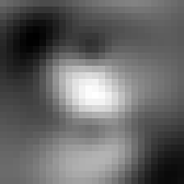
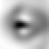
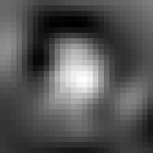
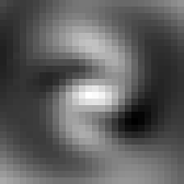
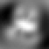
Figure 2: Learned dictionary corresponding to digits $0$ to $9$ from left to right.

7 Concluding Remarks

In this paper, we study the problem of learning a dictionary invariant to a pre-specified group of symmetries through the lens of representation theory. Using the representation theory of compact groups, we describe a recipe for learning dictionaries invariant to compact group symmetries. We briefly examine the harmonic analytical aspects of the dictionary learning problem, and we describe in detail the program for the groups SO(2), O(2), and SO(3).

In what follows, we briefly remark on important future directions that stem from our work.

Incorporating symmetries versus data augmentation. Symmetries and invariances in data arise very naturally in numerous application domains. Many successful representation techniques take advantage of this basic observation in some form or another. Fundamentally, this paper is guided by the philosophy that it is useful to incorporate the appropriate symmetries and invariances in the structure of the data representation we learn. Admittedly, the more typical response in similar settings is data augmentation – in simple terms, the data analyst appends transformed copies of the original dataset in the hope that the learned model has the appropriate invariant properties (for instance, one might hope a classifier predict the same outcome for any rotation of the same image).

The basic reason why data augmentation is widely used is that it is simple and cheap. However, we have no control over whether the learned model is truly invariant – it never truly ‘realizes’ that it is intended to be invariant. The computational methods we introduce here are powerful in that it learns representations that enforce invariance – the price we pay is computation cost. Are there application domains where the importance of incorporating the appropriate invariant structures in the learned data representation models sufficiently justify the additional computational cost required to train it? This is a basic question in representation learning that warrants further study.

Learning localized patches. A very closely variant of the problem formulation in 5 is to view the dictionary elements as localized patches or filters. In this formulation, we view the data as a single vector $y\in\mathbb{R}^{\tilde{d}}$ residing in very high dimensions – for instance, this could be a photograph or a single time series. The goal is to learn a collection of filters $\{\phi_{j}\}_{i=1}^{q}\subset\mathbb{R}^{\tilde{d}}$ that are only supported over $d\ll\tilde{d}$ consecutive coordinates – this is why these patches are localized.

From a mathematical and a conceptual perspective, these problems are identical – the techniques developed in this paper follow in a straightforward fashion to the more general setting. From a computational perspective, the fact that these patches are embedded in a much higher dimensional space $\mathbb{R}^{\tilde{d}}$ introduces challenges that we need to address. First, data dimension is effectively $\mathbb{R}^{d}$, and so $\rho(g)$ resides in a much higher dimensional space. Second, our framework advocates working in the Fourier domain for computational reasons. However, a spatially localized signal will not be localized in the frequency domain. It would be interesting to bring in techniques from numerical optimization and computational harmonic analysis to address these challenges.

SO(3) orbitopes. An outstanding unresolved question in this paper is if the SO(3) orbitope is tractable to express. Closely related to this set is the tensor nuclear norm ball restricted to tensors with block Toeplitz structure. While the tensor nuclear norm is known to be intractable to describe [19], there are principled methods for deriving tractable convex relaxations – one such scheme is based on the sum-of-squares hierarchy in which these relaxations are specified as the solution of a SDP [33]. It would be interesting to further investigate these connections.

Conic Programming Descriptions of Orbitopes. In Section 1, we stated that one of our main contributions is to provide a recipe for describing $\rho(g)$ explicitly. This still leaves an unresolved question – namely – how do we provide descriptions of the convex hull of $\{\rho(g):G\}$ that are amenable to optimization? Answering this question in full generality is most certainly out of reach. A more modest goal could be to provide a procedure for obtaining conic programming-based descriptions of structured classes of orbitopes, for instance, when the generators are known.

Appendix A Proofs of Theorem 4.1 and 4.3

We begin with some preparatory observations. As before, $\hat{H}\subseteq\hat{G}$ denotes a subset of irreducibles.

First, given $f\in L^{2}(\hat{G})$, we denote its projection onto $L^{2}(\hat{H})$ by $P_{L^{2}(\hat{H})}(f)$. Recall from 11 that the Fourier series expansion of $f$ is given by

$$f(x)~{}=~{}\sum_{\xi\in\hat{G}}\mathrm{dim}(V_{\xi})~{}\left\langle\hat{f}(\xi),\rho_{\xi}(x)^{*}\right\rangle_{\xi}~{}=~{}\sum_{\xi\in\hat{G}}\mathrm{dim}(V_{\xi})~{}\mathrm{tr}_{V_{\xi}}(\hat{f}(\xi)\rho_{\xi}(x)).$$

Because the Fourier functions form an orthogonal basis of $L^{2}(\hat{G})$, it follows that the Fourier series expansion of $P_{L^{2}(\hat{H})}(f)$ is simply the truncated expansion up to terms in $\hat{H}$

$$[P_{L^{2}(\hat{H})}(f)](x)~{}=~{}\sum_{\xi\in\hat{H}}\mathrm{dim}(V_{\xi})~{}\left\langle\hat{f}(\xi),\rho_{\xi}(x)^{*}\right\rangle_{\xi}~{}=~{}\sum_{\xi\in\hat{H}}\mathrm{dim}(V_{\xi})~{}\mathrm{tr}_{V_{\xi}}(\hat{f}(\xi)\rho_{\xi}(x)).$$ (47)

Second, and in a similar fashion, given an operator $t\in B(L^{2}(\hat{G}))$, we denote its projection onto $B(L^{2}(\hat{H}))$ by $P_{B(L^{2}(\hat{H}))}(t)$. Suppose $t$ is a block diagonal operator that acts on the Fourier coefficients by right multiplication

$$t:\hat{f}(\xi)\mapsto\hat{f}(\xi)t_{\xi},\qquad\text{ where }\quad t_{\xi}\in\mathbb{C}^{\mathrm{dim}(V_{\xi})\times\mathrm{dim}(V_{\xi})},\quad\xi\in\hat{G}.$$

In particular (and as a reminder), a consequence of Peter-Weyl’s is that the learned operators $\ell$ will obey such structure. Then the projection of $t$ will also obey the same block diagonal structure, but restricted to the terms in $\hat{H}$

$$P_{B(L^{2}(\hat{H}))}(t):\hat{f}(\xi)\mapsto\hat{f}(\xi)t_{\xi},\qquad\xi\in\hat{H}.$$ (48)

Proposition A.1.

Let $t\in B(L^{2}(\hat{G}))$. Then

$$\|P_{B(L^{2}(\hat{H}))}(t)\|^{+}_{\hat{H}}\leq\|t\|^{+}_{\hat{G}}.$$

Proof of Proposition A.1.

By noting that $t$ is a feasible solution to the argument in the definition in 30, we have

$$\|P_{B(L^{2}(\hat{H}))}(t)\|^{+}_{\hat{H}}=\inf\{\|z\|_{\hat{G}}:P_{B(L^{2}(\hat{H}))}(z)=t,z\in B(L^{2}(\hat{G}))\}\leq\|t\|_{\hat{G}}.$$

∎

Proposition A.2.

Let $\hat{H}\subseteq\hat{G}$ be subset of irreducibles. Let $\mathrm{OPT-}\hat{H}$ be the optimal value of 31, and let and $\mathrm{OPT-}\hat{G}$ be the optimal value of 32 (as a reminder, this is the same as 31 but over the full set of irreducibles $\hat{G}$). Then $\mathrm{OPT-}\hat{H}\leq\mathrm{OPT-}\hat{G}$.

Proof of Proposition A.2.

Let $\hat{\phi}^{\hat{G}}\in L^{2}(\hat{G})$ and $\ell^{\hat{G}}\in B(L^{2}(\hat{G}))$ be a pair of feasible solutions to 32. Let the corresponding objective value be $\mathrm{VAL}$.

Next, we substitute the pair of solutions $P_{L^{2}(\hat{H})}(\hat{\phi}^{\hat{G}})$ and $P_{B(L^{2}(\hat{H}))}(\ell^{\hat{G}})$ to 32, and we compare its corresponding objective value with $\mathrm{VAL}$.

First, by comparing the first term in 31 and in 32, we have

$$\sum_{\xi\in\hat{H}}\mathrm{dim}(V_{\xi})^{2}\|\hat{y}_{\xi}-\sum_{j=1}^{q}[P_{L^{2}(\hat{H})}(\hat{\phi}^{\hat{G}})]_{j,\xi}[P_{B(L^{2}(\hat{H}))}(\ell^{\hat{G}})]^{*}_{j,\xi}\|_{F}^{2}$$

$$={} \sum_{\xi\in\hat{H}}\mathrm{dim}(V_{\xi})^{2}\|\hat{y}_{\xi}-\sum_{j=1}^{q}\hat{\phi}^{\hat{G}}_{j,\xi}\ell^{\hat{G}*}_{j,\xi}\|_{F}^{2}$$

$$\leq{} \sum_{\xi\in\hat{G}}\mathrm{dim}(V_{\xi})^{2}\|\hat{y}_{\xi}-\sum_{j=1}^{q}\hat{\phi}^{\hat{G}}_{j,\xi}\ell^{\hat{G}*}_{j,\xi}\|_{F}^{2}.$$

The first equality is a consequence of 47 and 48.

Second, by Proposition A.1, we have $\|P_{B(L^{2}(\hat{H}))}(\ell^{\hat{G}})\|^{+}_{\hat{H}}\leq\|\ell^{\hat{G}}\|^{+}_{\hat{G}}$.

Third, we have

$$\sum_{\xi\in\hat{H}}\mathrm{dim}(V_{\xi})^{2}\|P_{L^{2}(\hat{H})}(\hat{\phi}^{\hat{G}})_{\xi}\|_{F}^{2}~{}=~{}\sum_{\xi\in\hat{H}}\mathrm{dim}(V_{\xi})^{2}\|\hat{\phi}^{\hat{G}}_{\xi}\|_{F}^{2}~{}\leq~{}\sum_{\xi\in\hat{G}}\mathrm{dim}(V_{\xi})^{2}\|\hat{\phi}^{\hat{G}}_{\xi}\|_{F}^{2}.$$

By summing these three inequalities, the pair of solutions $P_{L^{2}(\hat{H})}(\hat{\phi}^{\hat{G}})$ and $P_{B(L^{2}(\hat{H}))}(\ell^{\hat{G}})$ attain an objective value at most $\mathrm{VAL}$ in 31. The result follows by taking the infimum over all feasible $\hat{\phi}^{\hat{G}}$ and $\ell^{\hat{G}}$. ∎

Let $\hat{\Phi}^{\hat{H}}:=\{\hat{\phi}^{\hat{H}}_{1},\ldots,\hat{\phi}^{\hat{H}}_{q}\}\subset L^{2}(\hat{H})$ be the optimal dictionary, and $\{\ell^{(i)\hat{H}}_{j}\}_{1\leq i\leq n,1\leq j\leq q}\}\subset B(L^{2}(\hat{H}))$ be the optimal operators to 31. As discussed in Section 4, one can embed $\hat{\Phi}^{\hat{H}}$ into $L^{2}(\hat{G})$ in the natural way, and we let $\hat{\Phi}^{\hat{H}}$ denote such an embedding. As discussed also in Section 4, we choose the embedding of $\{\ell^{(i)\hat{H}}_{j}\}$ into $B(L^{2}(\hat{G}))$ to be such that $\|\ell^{\hat{H}}\|_{\hat{G}}=\|\ell^{\hat{H}}\|_{\hat{H}}$.

Proof of Theorem 4.1 and 4.2.

Let $\hat{\phi}^{\hat{H}}$ and $\hat{\ell}^{\hat{H}}$ denote the optimal dictionary elements and operators in 31. We consider what happens when we substitute these into the objective 32.

First, we have

$$\sum_{\xi\in\hat{G}}\frac{\mathrm{dim}(V_{\xi})^{2}}{2}\|\hat{y}_{\xi}-\sum_{j=1}^{q}\hat{\phi}^{\hat{H}}_{j,\xi}(\ell^{\hat{H}}_{j,\xi})^{*}\|_{F}^{2}$$

$$={}{} \sum_{\xi\in\hat{H}}\frac{\mathrm{dim}(V_{\xi})^{2}}{2}\|\hat{y}_{\xi}-\sum_{j=1}^{q}\hat{\phi}^{\hat{H}}_{j,\xi}(\ell^{\hat{H}}_{j,\xi})^{*}\|_{F}^{2}+\sum_{\xi\in\hat{G}\backslash\hat{H}}\frac{\mathrm{dim}(V_{\xi})^{2}}{2}\|\hat{y}_{\xi}\|_{F}^{2}.$$

Second, we have $\|\ell_{j}^{\hat{H}}\|_{\hat{G}}=\|\ell_{j}^{\hat{H}}\|^{+}_{\hat{H}}$, as we noted earlier.

Third, we have

$$\sum_{\xi\in\hat{G}}\mathrm{dim}(V_{\xi})^{2}\|\hat{\phi}^{\hat{H}}_{\xi}\|_{F}^{2}=\sum_{\xi\in\hat{H}}\mathrm{dim}(V_{\xi})^{2}\|\hat{\phi}^{\hat{H}}_{\xi}\|_{F}^{2}$$

because $\hat{\phi}^{\hat{H}}\in L^{2}(\hat{H})$.

Let $\epsilon_{\hat{H}}^{(i)}=\sum_{\xi\in\hat{G}\backslash\hat{H}}\frac{\mathrm{dim}(V_{\xi})^{2}}{2}\|\hat{y}^{(i)}_{\xi}\|_{F}^{2}$. By summing up the three components above, we have $\mathrm{OPT}-\hat{H}+\sum_{i}\epsilon_{\hat{H}}^{(i)}=\mathrm{OBJ}-\hat{H}$. By optimality of $\hat{\Phi}^{\hat{G}}$, we have $\mathrm{OBJ}-\hat{H}\geq\mathrm{OPT}-\hat{G}$. By Proposition A.2, we have $\mathrm{OPT}-\hat{G}\geq\mathrm{OPT}-\hat{H}$. Combining these, we have

$$\mathrm{OPT}-\hat{H}+\sum_{i}\epsilon_{\hat{H}}^{(i)}=\mathrm{OBJ}-\hat{H}\geq\mathrm{OPT}-\hat{G}\geq\mathrm{OPT}-\hat{H}.$$

Since the data $y$ has finite $\ell_{2}$-norm, we have $\sum\epsilon_{\hat{H}_{k}}^{(i)}\rightarrow 0$ as $\hat{H}_{k}\uparrow\hat{G}$. It follows that $\mathrm{OPT}-\hat{H}_{k}\uparrow\mathrm{OPT}-\hat{G}$ and $\mathrm{OBJ}-\hat{H}_{k}\downarrow\mathrm{OPT}-\hat{G}$. ∎

Proof of Theorem 4.3.

By Theorem 4.2, we have $\mathrm{OPT}-\hat{H}_{k}\downarrow\mathrm{OPT}-\hat{G}$. In particular, it guarantees that $\mathrm{OPT}-\hat{H}_{k}\leq\mathrm{OPT}+\epsilon$ eventually. Then by canonical uniqueness $D(\hat{\Phi},\hat{\Phi}^{\hat{H}_{k}})\leq\delta(\epsilon)$. Then take $\epsilon\rightarrow 0$ so that $\delta(\epsilon)\rightarrow 0$, from which the result follows. ∎

Appendix B Learning O(2) Invariant Dictionaries

In this section, we describe the full program of learning a dictionary that is invariant to O(2). One example of an application is for images that are invariant under rotations about the origin and reflections about any line through the origin. Our discussion serves as a companion to the earlier discussion for the group SO(2) in Section 5.2.

Irreducible representations. Concretely, consider the matrix group with elements of the form

$$\left\{R(\theta):=\left(\begin{array}[]{cc}\cos\theta&\sin\theta\\ -\sin\theta&\cos\theta\end{array}\right),L(\theta):=\left(\begin{array}[]{cc}\cos\theta&\sin\theta\\ \sin\theta&-\cos\theta\end{array}\right):\theta\in[0,2\pi)\right\}.$$

The irreducible representations are the mappings $\rho_{k}:(R(\theta),L(\theta))\mapsto(\rho_{R,k}(\theta),\rho_{L,k}(\theta))$, where

$$\rho_{R,k}(\theta)=\left(\begin{array}[]{cc}\exp(ik\theta)&\\ &\exp(-ik\theta)\end{array}\right),\qquad\rho_{L,k}(\theta)=\left(\begin{array}[]{cc}&\exp(ik\theta)\\ \exp(-ik\theta)&\end{array}\right).$$

The irreducible representations are all two-dimensional, except the trivial one corresponding to $k=0$. The Fourier coefficients are $2\times 2$ complex matrices, and every function over O(2) can be expressed as

$$f(g)=c_{0}+\sum_{k=1}^{\infty}2\mathrm{tr}(C_{k}\rho_{k}(g)),\qquad g\in O(2),$$ (49)

where $C_{k}$ are the matrix-valued Fourier coefficients.

Atomic norm. Truncate the basis by taking the upper limit in 49 to be $N$. Then the action by an element in O(2) is the block operator

$$(1,\rho_{1}(\theta),\ldots,\rho_{N}(\theta)).$$

Consider an operator of the form

$$Z:=(z_{0},Z_{1},\ldots,Z_{N})\in\mathbb{R}\times(\mathbb{C}^{2\times 2})^{\otimes N}.$$

The atomic norm is given by

$$\begin{aligned} \left\|Z\right\|_{\tilde{G}}~{}~{}=&~{}~{}\inf\quad z_{L,+,0}+z_{L,-,0}+z_{R,+,0}+z_{R,-,0}\\ &~{}~{}\mathrm{s.t.}\quad\mathbf{z}_{L}=\mathbf{z}_{L,+}-\mathbf{z}_{L,-},~{}~{}\mathbf{z}_{R}=\mathbf{z}_{R,+}-\mathbf{z}_{R,-}\\ &\quad\quad\quad Z=\left(z_{R,0}+z_{L,0},\left(\begin{array}[]{cc}z_{R,1}&z_{L,1}\\ z_{L,-1}&z_{R,-1}\end{array}\right),\ldots,\left(\begin{array}[]{cc}z_{R,N}&z_{L,N}\\ z_{L,-N}&z_{R,-N}\end{array}\right)\right)\\ &\quad\quad\quad\mathbf{z}_{L,+},\mathbf{z}_{L,-},\mathbf{z}_{R,+},\mathbf{z}_{R,-}\in\mathcal{C}_{N}\end{aligned}.$$

Appendix C Experimental Details of Section 6.4

In this section, we describe the details of our numerical experiment in Section 6.4.

Data. Our raw dataset are handwritten digits from the MNIST dataset [12]. These are $28\times 28$-pixel images of hand-written digits from $0$ to $9$ in grayscale with values ranging from $0$ (for black) to $1$ (for white). We apply a sequence of pre-processing steps to convert these handwritten digits to functions over SO(3) to apply our procedure. First, we translate these images so the cartesian coordinates are $[-\sqrt{2},\sqrt{2}]\times[-\sqrt{2},\sqrt{2}]$. Second, we define a function $h:S^{2}\rightarrow\mathbb{R}$ so that

$$h((x,y,z)^{T}):=\text{Image Intensity at }(x/(1+z),y/(1+z)).$$

The intensity values of $h$ are initially specified only on a lattice grid – these correspond to locations of the pixels of the original image. For points off the lattice grid $(x,y)$ but within the domain $[-1/\sqrt{2},1/\sqrt{2}]\times[-1/\sqrt{2},1/\sqrt{2}]$, we define the value of $h$ via a bilinear interpolation using the four lattice points $(\lfloor x\rfloor,\lfloor y\rfloor),(\lceil x\rceil,\lfloor y\rfloor),(\lfloor x\rfloor,\lceil y\rceil),(\lceil x\rceil,\lceil y\rceil)$. As for values of $x,y$ that fall outside the domain $[-1/\sqrt{2},1/\sqrt{2}]\times[-1/\sqrt{2},1/\sqrt{2}]$, we define the value of $h$ to be $0$. Third, we define function $f:\text{SO}(3)\rightarrow\mathbb{R}$ by

$$f(\left(\begin{array}[]{c|c|c}u&v&w\end{array}\right)):=h(u)\qquad\text{where}\qquad u,v,w\in S^{2}.$$

Here, we identify an element in SO(3) by a $3\times 3$-dimensional matrix whose columns are $u,v,w$. Fourth, we compute the Fourier coefficients corresponding to $f$, which we denote by $\hat{y}$. Recall $\hat{y}$ is a countable sequence of complex matrices of size $(2j+1)\times(2j+1)$, indexed by $j\in\{0,1,\ldots\}$. In our implementation, we truncated the Fourier series to $j\in\{0,1,\ldots,10\}$.

Numerical Experiment. We apply our dictionary learning procedure to learn a dictionary comprising one dictionary element $\hat{\phi}_{\rm opt}$ for the digits $\{0,1,\ldots,9\}$. For each digit, our dataset comprises $200$ images. We perform $10$ outerloop iterations in our dictionary learning procedure.

Results. The computed dictionary elements are Fourier coefficients. To visualize these as images, we need to reverse the pre-processing steps. Let $\hat{\phi}_{\rm opt}$ be a dictionary element. First, we perform the inverse Fourier transform to obtain $\phi_{\rm opt}\in L^{2}(\mathrm{SO}(3))$. Second, define the spherical image $h_{\rm opt}$ corresponding to $\phi_{\rm opt}$ by

$$h_{\rm opt}(u)=\int_{R:R=(u|*|*)}\phi_{\rm opt}(R)\mu(dR).$$

Here, $\mu$ is the uniform measure. To approximate this integral, notice that – assuming $u$ is at the north-pole – the remaining columns lie on the equator. We set the second argument – say $v$ – to be equally spaced points on the equator, and we set the third argument – say $w$ – to be $w=\pm(u\times v)$. Finally, the pixel intensity of the learned dictionary at location $x,y$, $-1/\sqrt{2}\leq x,y\leq 1/\sqrt{2}$, is given by $\hat{h}((x,y,\sqrt{1-x^{2}-y^{2}})^{T})$.

In Figure 2, we show the learned dictionary elements for the digits $0$ to $9$. For digits $0$, $1$ and $5$, we note some resemblance between the learned dictionary element and the actual digit; for the other digits, the resemblance is less clear. (We also note that the dictionary elements for the digits $6$ and $9$ bear similarities not observed in other digits.) This can be explained by a couple of reasons: For instance digits $0$ and $1$ are structurally quite ‘simple’ in that $0$ is a single circle while $1$ is a single stroke, and that makes it easier for the dictionary learning algorithm to identify such structures; the remaining digits are more complex. Another reason is that the Euclidean loss, while amenable to computation, is not the ideal loss function for image processing – alternatives such as the Wasserstein distances are better suited for images, though they lead to algorithms that are computationally far more expensive. We note in passing that the objects in Figure 2 are dictionary elements, whose linear combinations would be relevant for digits in the MNIST problem. It is not apparently evident if the dictionary elements themselves should possess any interpretable structure in the context of the actual digits.

Computational considerations. We make some brief remarks concerning the computational aspects of our experiment. A consequence of the function $f$ being real-valued is that the $j$-th matrix coefficient $\hat{y}:=\hat{y}_{\xi=j}\in\mathbb{C}^{(2j+1)\times(2j+1)}$ (here, the index runs between $-j$ and $j$) satisfies the relation

$$X_{-m,-m^{\prime}}=(-1)^{j}X_{-m,m^{\prime}}=(-1)^{j+m+m^{\prime}}X_{m,-m^{\prime}}^{*}=(-1)^{m+m^{\prime}}X_{m,m^{\prime}}.$$

The degrees of freedom within the $j$-th matrix is $(2j+1)(j+1)$ for $j$ even and $2j^{2}+j$ for $j$ odd. Hence, in truncating the data to Fourier coefficients in $j\in\{0,1,\ldots,10\}$, the ambient (real) dimension in our problem is $891$, which is comparable to datasets in prior works. Our earlier proposal – that is, the relaxations described in Section 6.2 – requires solving a SDP over matrices in $21^{3}\times 21^{3}$ dimensions per data-point. This is near the limit of what general purpose SDP solvers are able to solve in a single instance, much less repeated over the dataset and multiple interations.

References

- [1] Amit Agrawal, Ramesh Raskar, and Rama Chellappa. What is the range of surface reconstructions from a gradient field? In European conference on computer vision, pages 578–591. Springer, 2006.
- [2] Afonso S Bandeira, Moses Charikar, Amit Singer, and Andy Zhu. Multireference alignment using semidefinite programming. In Proceedings of the 5th conference on Innovations in theoretical computer science, pages 459–470, 2014.
- [3] Tamir Bendory, Alberto Bartesaghi, and Amit Singer. Single-particle cryo-electron microscopy: Mathematical theory, computational challenges, and opportunities. IEEE signal processing magazine, 37(2):58–76, 2020.
- [4] B. N. Bhaskar, G. Tang, and B. Recht. Atomic Norm Denoising with Applications to Line Spectral Estimation. IEEE Transactions on Signal Processing, 61(23):5987–5999, 2013.
- [5] T. Blumensath and M. E. Davies. Sparse and Shift-Invariant Representations of Music. IEEE Transactions on Audio, Speech, and Language Processing, 14(1), 2006.
- [6] E. J. Candès, J. Romberg, and T. Tao. Robust Uncertainty Principles: Exact Signal Reconstruction from Highly Incomplete Frequency Information. IEEE Transactions on Information Theory, 52(2):489–509, 2006.
- [7] E. J. Candès and T. Tao. Near-Optimal Signal Recovery From Random Projections: Universal Encoding Strategies? IEEE Transactions on Information Theory, 52(12):5406–5425, 2006.
- [8] C. Carathéodory. Über den variabilitätsbereich der fourierschen konstanten von positiven harmonischen funktionen. Rendiconti del Circolo Matematico di Palermo, 32(1), 1911.
- [9] C. Carathéodory and L. Fejér. Über den zusammenhang der extremen von harmonischen funktionen mit ihren koeffizienten und über den picard-landauschen satz. Rendiconti del Circolo Matematico di Palermo, 32(1), 1911.
- [10] V. Chandrasekaran, B. Recht, P. A. Parrilo, and A. S. Willsky. The Convex Geometry of Linear Inverse Problems. Foundations of Computational Mathematics, 12(6):805–849, 2012.
- [11] S. S. Chen, D. L. Donoho, and M. A. Saunders. Atomic Decomposition by Basis Pursuit. SIAM Journal on Scientific Computing, 20(1):33–61, 1998.
- [12] L. Deng. The MNIST Database of Handwritten Digit Images for Machine Learning Research. IEEE Signal Processing Magazine, 29(6):141–142, 2012.
- [13] D. L. Donoho. De-noising by Soft-Thresholding. IEEE Transactions on Information Theory, 41(3):613–627, 1995.
- [14] D. L. Donoho. Compressed Sensing. IEEE Transactions on Information Theory, 52(4):1289–1306, 2006.
- [15] D. L. Donoho and X. Huo. Uncertainty Principles and Ideal Atomic Decomposition. IEEE Transactions on Information Theory, 47(7):2845–2862, 2001.
- [16] M. Elad. Sparse and Redundant Representations: From Theory to Applications in Signal and Image Processing. Springer, 2010.
- [17] C. Esteves, C. Allen-Blanchette, A. Makadia, and K. Daniilidis. Learning SO(3) Equivariant Representations with Spherical CNNs. In Proceedings of the European Conference on Computer Vision (ECCV), pages 52–68, 2018.
- [18] Zhou Fan, Yi Sun, Tianhao Wang, and Yihong Wu. Likelihood landscape and maximum likelihood estimation for the discrete orbit recovery model. arXiv preprint arXiv:2004.00041, 2020.
- [19] S. Friedland and L.-H. Lim. Nuclear Norm of Higher-order Tensors. Mathematics of Computation, 87(311), 2018.
- [20] C. Garcia-Cardona and B. Wohlberg. Convolutional Dictionary Learning: A Comparative Review and New Algorithms. IEEE Transactions on Computational Imaging, 4(3), 2018.
- [21] Subhroshekhar Ghosh and Philippe Rigollet. Sparse multi-reference alignment: Phase retrieval, uniform uncertainty principles and the beltway problem. Foundations of Computational Mathematics, pages 1–48, 2022.
- [22] Arvind Giridhar and Praveen R Kumar. Distributed clock synchronization over wireless networks: Algorithms and analysis. In Proceedings of the 45th IEEE Conference on Decision and Control, pages 4915–4920. IEEE, 2006.
- [23] R. Grosse, R. Raina, H. Kwong, and A. Y. Ng. Shift-invariant Sparse Coding for Audio Classification. In Proceedings of the Twenty-Third Conference on Uncertainty in Artificial Intelligence, 2007.
- [24] Roei Herzig, Moshiko Raboh, Gal Chechik, Jonathan Berant, and Amir Globerson. Mapping images to scene graphs with permutation-invariant structured prediction. arXiv preprint arXiv:1802.05451, 2018.
- [25] P. Jost, P. Vandergheynst, S. Lesage, and R. Gribonval. MoTIF : An Efficient Algorithm for Learning Translation Invariant Dictionaries. In Proceedings of the International Conference on Acoustics, Speech, and Signal Processing (ICASSP), 2006.
- [26] Ramakrishna Kakarala. The bispectrum as a source of phase-sensitive invariants for fourier descriptors: a group-theoretic approach. Journal of Mathematical Imaging and Vision, 44(3):341–353, 2012.
- [27] R. Kondor. A Novel Set of Rotationally and Translationally Invariant Features for Images Based on the Non-commutative Bispectrum. arXiv preprint cs/0701127, 2007.
- [28] R. Kondor. Group Theoretical Methods in Machine Learning. PhD thesis, Columbia University, 2008.
- [29] M. S. Lewicki and T. J. Sejnowski. Coding Time-varying Signals using Sparse, Shift-invariant Representations. In Proceedings of the 1998 Conference on Advances in Neural Information Processing Systems II, 1998.
- [30] J. Liu, C. Garcia-Cardona, B. Wohlberg, and W. Yin. First- and Second-Order Methods for Online Convolutional Dictionary Learning. SIAM Journal on Imaging Sciences, 11(2), 2018.
- [31] Tobias Moroder, Philipp Hyllus, Géza Tóth, Christian Schwemmer, Alexander Niggebaum, Stefanie Gaile, Otfried Gühne, and Harald Weinfurter. Permutationally invariant state reconstruction. New Journal of Physics, 14(10):105001, 2012.
- [32] Y. Nesterov and A. Nemirovskii. Interior-Point Polynomial Algorithms in Convex Programming. SIAM Studies in Applied and Numerical Mathematics, 1994.
- [33] J. Nie. Symmetric Tensor Nuclear Norms. SIAM Journal on Applied Algebraic Geometry, 1:599–625, 2017.
- [34] B. A. Olshausen and D. J. Field. Emergence of Simple-Cell Receptive Field Properties by Learning a Sparse Code for Natural Images. Nature, 381:607–609, 1996.
- [35] B. A. Olshausen and D. J. Field. Sparse Coding with an Overcomplete Basis Set: A Strategy Employed by V1? Vision Research, 37(23):3311–3325, 1997.
- [36] V. Papyan, Y. Romano, J. Sulam, and M. Elad. Convolutional Dictionary Learning via Local Processing. In The IEEE International Conference on Computer Vision, 2017.
- [37] Amelia Perry, Jonathan Weed, Afonso S Bandeira, Philippe Rigollet, and Amit Singer. The sample complexity of multireference alignment. SIAM Journal on Mathematics of Data Science, 1(3):497–517, 2019.
- [38] M. D. Plumbley, S. A. Abdallah, T. Blumensath, and M. E. Davies. Sparse Representations of Polyphonic Music. Signal Processing, 86(3), 2006.
- [39] J. Renegar. A Mathematical View of Interior-Point Methods in Convex Optimization. MOS-SIAM Series on Optimization, 2001.
- [40] David M Rosen, Luca Carlone, Afonso S Bandeira, and John J Leonard. A certifiably correct algorithm for synchronization over the special euclidean group. In Algorithmic Foundations of Robotics XII, pages 64–79. Springer, 2020.
- [41] C. Rusu. On Learning with Shift-invariant Structures. Digital Signal Processing, 99, 2020.
- [42] R. Sanyal, F. Sottile, and B. Sturmfels. Orbitopes. Mathematika, 57(2):275–314, 2011.
- [43] Amit Singer et al. Mathematics for cryo-electron microscopy. arXiv preprint arXiv:1803.06714, 2018.
- [44] Y. S. Soh. Group Invariant Dictionary Learning. IEEE Transactions on Signal Processing, 69:3612–3626, 2021.
- [45] A. H. Song, F. J. Flores, and D. Ba. Convolutional Dictionary Learning with Grid Refinement. IEEE Transactions on Signal Processing, 68:2558–2573, 2020.
- [46] O. Toeplitz. Zur theorie der quadratischen und bilinearen formen von unendlichvielen veränderlichen. Mathematische Annalen, 70(3), 1911.
- [47] DW Vasco. Invariance, groups, and non-uniqueness: the discrete case. Geophysical Journal International, 168(2):473–490, 2007.
- [48] B. Wohlberg. Efficient Algorithms for Convolutional Sparse Representations. IEEE Transactions on Image Processing, 25(1), 2015.
- [49] E. Zisselman, J. Sulam, and M. Elad. A Local Block Coordinate Descent Algorithm for the CSC Model. In IEEE/CVF Conference on Computer Vision and Pattern Recognition (CVPR), 2019.