(Semi-)device independently characterizing quantum temporal correlations

Abstract

We develop a framework for characterizing quantum temporal correlations in a general temporal scenario, in which an initial quantum state is measured, sent through a quantum channel, and finally measured again. This framework does not make any assumptions on the system nor on the measurements, namely, it is device-independent. It is versatile enough, however, to allow for the addition of further constraints in a semi-device-independent setting. Our framework serves as a natural tool for quantum certification in a temporal scenario when the quantum devices involved are uncharacterized or partially characterized. It can hence also be used for characterizing quantum temporal correlations when one assumes an additional constraint of no-signalling in time, there are upper bounds on the involved systems’ dimensions, rank constraints – for which we prove genuine quantum separations over local hidden variable models – or further linear constraints. We present a number of applications, including bounding the maximal violation of temporal Bell inequalities, quantifying temporal steerability, bounding the maximum successful probability in a scenario of quantum randomness access codes.

Quantum mechanics features correlations between spatially separated systems that are stronger than attainable in physical systems following classical laws. Bell’s theorem  Bell (1964) limits correlations that classical local- hidden-variable models can exhibit. This feature of quantum mechanics, also referred to as non-locality Brunner et al. (2014), is not only the defining feature that sets apart quantum from classical mechanics, it can also be exploited in technological-minded applications. Notably, it can be used in new modes of quantum certification that do not require any (possibly unwarranted) assumptions on the underlying states nor on the measurements involved. In such device-independent (DI) quantum certification Acín et al. (2007); Scarani (2012); Brunner et al. (2014), interestingly, data alone can be seen as being sufficient to certify properties. Along this line of thought, randomness certification Pironio et al. (2010), entanglement verification Liang et al. (2015); Baccari et al. (2017) and estimation Moroder et al. (2013), quantum state cerification Yang et al. (2014), steerability witnessing Chen et al. (2016a, 2018), and measurement incompatibility certification Chen et al. (2021a) have all been obtained through the observed non-local correlations only and no assumption has to be made on the shared quantum state nor the measurement involved. The Navascués-Pironio-Acín hierarchy Navascués et al. (2007, 2008); Doherty et al. (2008); Moroder et al. (2013) – building on earlier work Doherty et al. (2004); Eisert et al. (2004) – has been a key tool in these efforts. The framework of device independence is compelling, in that one learns about properties of quantum systems without having to make assumptions about the devices with which these properties are being assessed.

That said, the original Bell scenario referring to spatial correlations is by no means the only setting that certifies quantum features beyond what classical local-hidden-variable models can deliver. It has been extended to include temporal correlations, making reference to non-macro-realistic temporal correlations of single systems between two instances in time Emary et al. (2013); Vitagliano and Budroni (2022). Leggett and Garg Leggett and Garg (1985) have shown that, in quantum theory, there exists temporal correlations that are not macro-realistic, i.e., they do not admit the joint assumption of macroscopicity and non-invasive measurability. The original Leggett-Garg scenario is as follows: A quantum state is initially prepared and sent through a quantum channel. During the dynamics, the same measurement is performed at some, at least three, points in time. This has then been generalized to an identical preparation step, but followed by multiple choices of measurements at each point of time Brukner et al. (2004); Fritz (2010). Such a setting has been dubbed temporal Bell scenario, since one may view it as a temporal analogue of the standard Bell scenario. Unlike the Leggett-Garg scenario, in a temporal Bell scenario, measurement outcomes between two points of time are sufficient to observe non-macroscopic correlations. Like the situation in the Bell scenario, researchers are searching for a practical way to characterize quantum temporal correlations. The question is, given observed statistics in a temporal scheme, do there exist quantum states and measurements which reproduce such statistics? Steps have been taken to characterize quantum temporal correlations in the standard Leggett-Garg scenario Budroni et al. (2013). Nevertheless, characterizing quantum temporal correlations in the temporal Bell scenario remains an open problem, again with implications for device-independence. Indeed, it is not even known whether such an approach can be pursued at all.

In this work, we develop a framework based on what we call instrument moment matrices (IMMs) to characterize quantum temporal correlations in a temporal Bell scenario. The IMMs are matrices of expectation values of the post-measurement states, where measurements are described by instruments. By construction, if the initial state and the measurements follow quantum theory, the IMMs are positive semi-definite. As such, quantum temporal correlations can be characterized by semi-definite programming Boyd and Vandenberghe (2004). Besides, the characterization will be more accurate when the size of IMMs becomes larger (see Refs. Navascués et al. (2007, 2008) for the original idea behind such a hierarchical characterization and Refs. Moroder et al. (2013); Lang et al. (2014); Berta et al. (2016); Chen et al. (2016a, 2018); Bowles et al. (2020); Chen et al. (2021a); Lin et al. (2022) for some variants). Our characterization is implemented both in a fully device-independent (DI) and semi-DI fashion that incorporates partial knowledge about the devices: We generalize the reading of semi-DI settings of Ref. Liang et al. (2011) and advocate—complementing similarly motivated steps closer to the setting of fully specified devices of “semi-device-dependent” characterization Roth et al. (2023)—that this intermediate regime is highly reasonable and important. By DI we mean that the results are based on the observed temporal correlations only, but no measurements and channels have to be specified a-priori. In the temporal scenario, there is no way to rule out the possibility of sending information from an earlier time; therefore, we assume there are no side channels in our setting. In other words, we assume that we are not in an adversarial scenario such as in that of quantum key distribution. However, since the space of temporal correlations is so abundant that temporal quantum correlations can, in general, be realized by classical ones Clemente and Kofler (2016); Brierley et al. (2015), we have to add additional constraints to reveal quantum advantages. For this reason, we further consider 1) the constraint of no-signaling in time, 2) the constraint on the system’s dimension, and 3) the constraint on the system’s rank respectively. We show that IMMs allows us to characterize several quantum resources and tasks in a DI or semi-DI scenario. These includes computing an upper bound on the maximal violation of a temporal Bell inequality, estimating the minimum degree of temporal steerability, computing the maximum successful probability in a scenario of quantum randomness access codes, and identifying quantum state preparation. For including the rank constraint, to the best of our knowledge, this is the first work to enforce additional constraint apart from the dimensional constraint into a device-independent scenario. We would like to stress that in Ref. Navascués and Vértesi (2015), the general idea of characterizing temporal correlations has been proposed. The difference is that Ref. Navascués and Vértesi (2015) has focused on the prepare-and-measure scenario while we consider a two-time-measurement scenario ( see Fig. 1). Building on this, we demonstrate several explicit applications.

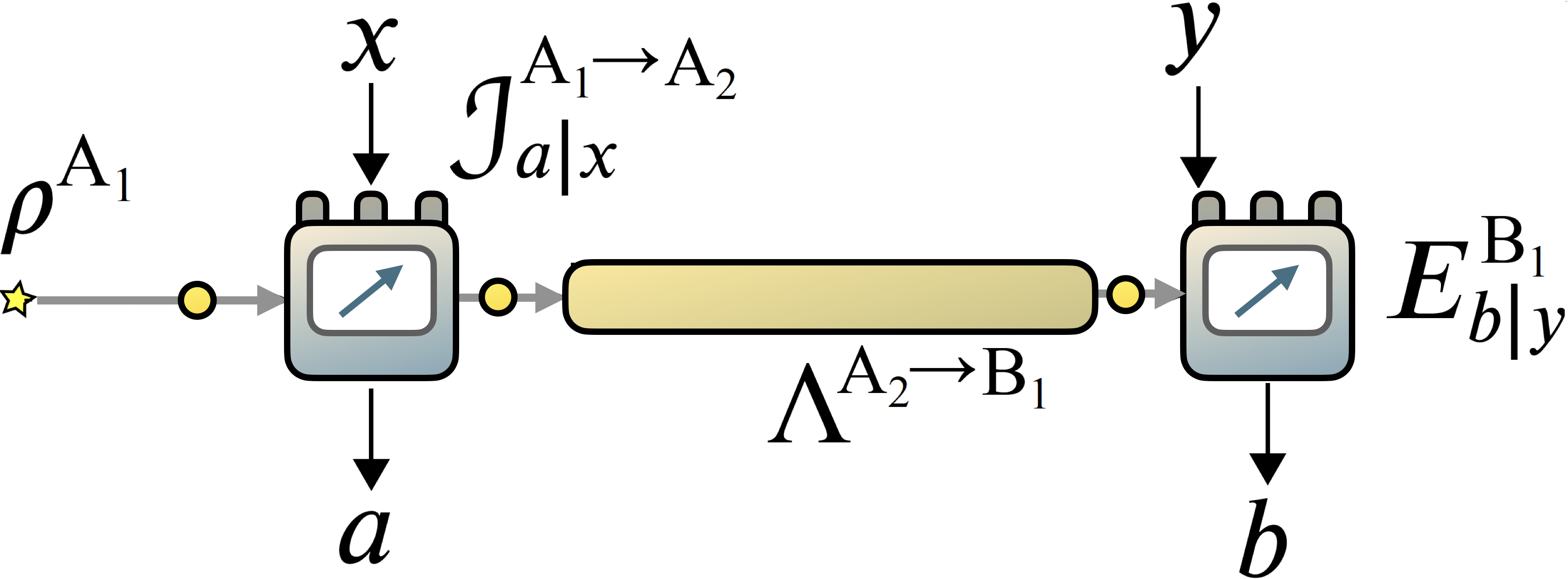
Figure 1: The scenario considered in this work.

The scenario. First, we introduce the notion of an instrument. An instrument $\{\mathcal{J}_{a}^{{\rm A}_{1}\rightarrow{\rm A}_{2}}\}$: $\mathcal{L}(\mathcal{H}_{{\rm A}_{1}})\rightarrow\mathcal{L}(\mathcal{H}_{{\rm A}_{2}})$ is a set of completely positive (CP) and trace non-increasing maps which maps a quantum state $\rho^{{\rm A}_{1}}$ to a post-measurement state $\mathcal{J}_{a}^{{\rm A}_{1}\rightarrow{\rm A}_{2}}(\rho^{{\rm A}_{1}})$ where $a\in\mathcal{A}=\{0,1,2,\dots\}$ can be treated as the assigned outcome associated with the state $\mathcal{J}_{a}^{{\rm A}_{1}\rightarrow{\rm A}_{2}}(\rho^{{\rm A}_{1}})$. The probability of obtaining the outcome $a$, denoted by $P(a)$, can be computed via $P(a)=\operatorname{tr}(\mathcal{J}_{a}^{{\rm A}_{1}\rightarrow{\rm A}_{2}}(\rho^{{\rm A}_{1}}))$, therefore one has $\operatorname{tr}\sum_{a}\mathcal{J}_{a}^{{\rm A}_{1}\rightarrow{\rm A}_{2}}(\rho^{{\rm A}_{1}})=\operatorname{tr}(\rho^{{\rm A}_{1}})$ due to the normalization.

In our scenario, we can choose different instruments to measure the state. We use the notation $\{\mathcal{J}_{a|x}^{{\rm A}_{1}\rightarrow{\rm A}_{2}}\}$ to denote the collection of instruments, where $x\in\mathcal{X}=\{0,1,2,\dots\}$ labels the choice of measurement settings (see Fig. 1). The post-measurement state $\mathcal{J}_{a|x}^{{\rm A}_{1}\rightarrow{\rm A}_{2}}(\rho^{{\rm A}_{1}})$ is then submitted into a quantum channel $\Lambda^{{\rm A}_{2}\rightarrow{\rm B}_{1}}$: $\mathcal{L}(\mathcal{H}_{{\rm A}_{2}})\rightarrow\mathcal{L}(\mathcal{H}_{{\rm B}_{1}})$. Finally, the evolved state is measured by another measurement. At this stage, we only care about the outcome, and hence the measurements can be described by positive operator-valued measures (POVMs) $\{E_{b|y}^{{\rm B}_{1}}\}$ that are positive semi-definite $E_{b|y}^{{\rm B}_{1}}\succeq 0$ and normalized as $\sum_{b}E_{b|y}^{{\rm B}_{1}}=\openone$, where $b\in\mathcal{B}$ and $y\in\mathcal{Y}$ denote the measurement outcome and setting, respectively. By repeating the above experiment many rounds, we will observe a set of probabilities $\{P(a,b|x,y):=P(b|a,x,y)P(a|x)\}$, termed temporal correlations. The temporal correlations can be obtained by applying the Born rule

$$P(a,b|x,y) = \operatorname{tr}\left\{E_{b|y}^{{\rm B}_{1}}\left[\Lambda^{{\rm A}_{2}\rightarrow{\rm B}_{1}}\left(\mathcal{J}_{a|x}^{{\rm A}_{1}\rightarrow{\rm A}_{2}}(\rho^{{\rm A}_{1}})\right)\right]\right\}$$ (1)

$$= \operatorname{tr}\bigl{[}E_{b|y}^{{\rm B}_{1}}\mathcal{I}_{a|x}^{{\rm A}_{1}\rightarrow{\rm B}_{1}}(\rho^{{\rm A}_{1}})\bigr{]}$$

where $\{\mathcal{I}_{a|x}^{{\rm A}_{1}\rightarrow{\rm B}_{1}}:=\Lambda^{{\rm A}_{2}\rightarrow{\rm B}_{1}}\circ\mathcal{J}_{a|x}^{{\rm A}_{1}\rightarrow{\rm A}_{2}}\}_{a}$ is a valid instrument for each $x$. In a temporal scenario, there exists an inherent constraint that a futural observer can not send any information to the past, i.e., the constraint of arrow of time, yielding $\sum_{b}P(a,b|x,y)=\sum_{b}P(a,b|x,y^{\prime})$ for all $y\neq y^{\prime}.$

The instrument moment matrices and their DI formulation. The instrument moment matrices (IMMs) are constructed by applying CP maps $\mathcal{E}$: $\mathcal{L}(\mathcal{H}_{{\rm B}_{1}})\rightarrow\mathcal{L}(\mathcal{H}_{\bar{{\rm B}}_{1}})$ on the post-measurement states $\mathcal{I}_{a|x}^{{\rm A}_{1}\rightarrow{\rm B}_{1}}(\rho^{{\rm A}_{1}})$, i.e., $\mathcal{E}(\mathcal{I}_{a|x}^{{\rm A}_{1}\rightarrow{\rm B}_{1}}(\rho^{{\rm A}_{1}}))=\sum_{n}K_{n}[\mathcal{I}_{a|x}^{{\rm A}_{1}\rightarrow{\rm B}_{1}}(\rho^{{\rm A}_{1}})]K_{n}^{\dagger}$ with $K_{n}:=\sum_{i}|i\rangle_{\bar{{\rm B}}_{1}{\rm B}_{1}}\langle n|S_{i}$ being the Kraus operators. Here, $\{|i\rangle_{\bar{{\rm B}}_{1}}\}$ and $\{|j\rangle_{{\rm B}_{1}}\}$ are orthonormal bases for the output space $\mathcal{H}_{\bar{{\rm B}}_{1}}$ and input space $\mathcal{H}_{{\rm B}_{1}}$, respectively. Following Ref. Moroder et al. (2013), given a level $\ell$ we choose $\{S_{i}\}$ as $\openone\cup\mathcal{S}^{(1)}\cup\mathcal{S}^{(2)}\cup\dots\cup\mathcal{S}^{(\ell)}$, where $\mathcal{S}^{(\ell)}$ is composed of the $\ell$th order products of the operators in the set $\{E_{b|y}^{{\rm B}_{1}}\}_{b=1,\dots,|\mathcal{B}|-1}^{y=1,\dots,|\mathcal{Y}|}$. The $\ell$th-level IMMs can be defined as

$$\chi_{a|x}^{(\ell)}:=\mathcal{E}[\mathcal{I}_{a|x}(\rho^{{\rm A}_{1}})]=\sum_{i,j}|i\rangle\langle j|\operatorname{tr}\left[\mathcal{I}_{a|x}(\rho^{{\rm A}_{1}})S_{j}^{\dagger}S_{i}\right].$$ (2)

Therefore, the entry of the $i$th row and $j$th column of $\chi_{a|x}^{(\ell)}$ can be treated as the “expectation value” of the product of $S_{j}^{\dagger}$ and $S_{i}$ given the state $\mathcal{I}_{a|x}^{{\rm A}_{1}\rightarrow{\rm B}_{1}}(\rho^{{\rm A}_{1}})$. In Appendix A, we explicitly provide an example of IMMs for dichotomic measurement settings and outcomes. Note that the IMMs are positive semi-definite whenever $\mathcal{I}_{a|x}$, $\rho$, $E_{b|y}^{{\rm B}_{1}}$ are quantum realizable: The set of constraints of positive semi-definiteness $\chi_{a|x}^{(\ell)}\succeq 0~{}\forall a,x$ serves as a natural characterization of the quantum set of temporal correlations $\{P(a,b|x,y)\}$. The characterization is improved when the level $\ell$ increases. Depending on the scenario under consideration, the improvement is hard to be observed from a level $\ell_{c}$ and we say $\chi_{a|x}^{(\ell_{c})}$ provides a proper approximation of the quantum set of temporal correlations. We will from now on use the notation $\chi_{a|x}$ to simply denote $\chi_{a|x}^{(\ell)}$.

When focusing on temporal correlations, quantum systems do not “outperform” classical systems in that a classical system with a sufficiently high dimension carries information which allows observers at later time to obtain. The simplest scheme is that an observer at earlier time can just send all the information about the measurement settings and outcomes to an observer at later time, then the correlation space will be filled by such a strategy. To let quantum systems demonstrate their superior performance, a constraint is to limit the dimension of the underlying system. By doing so, it has been shown that quantum systems outperform classical systems with the same dimension Gallego et al. (2010). If we require that the entire system is embedded in dimension at most $d$, we have $P(a,b|x,y)=\operatorname{tr}\{E_{b|y}^{{\rm B}_{1}}[\mathcal{I}_{a|x}^{{\rm A}_{1}\rightarrow{\rm B}_{1}}(\rho^{{\rm A}_{1}})]\},$ with $\rho^{{\rm A}_{1}}\in\mathcal{L}(\mathcal{H}_{d}^{{\rm A}_{1}})$, $\mathcal{I}_{a|x}^{{\rm A}_{1}\rightarrow{\rm B}_{1}}:\mathcal{L}(\mathcal{H}_{d}^{{\rm A}_{1}})\rightarrow\mathcal{L}(\mathcal{H}_{d}^{{\rm B}_{1}})$, and $E_{b|y}^{{\rm B}_{1}}\in\mathcal{D}(\mathcal{H}_{d}^{{\rm B}_{1}})$. Following the idea of Ref. Navascués and Vértesi (2015), the set of probabilities $P(a,b|x,y)$ generated by $d$-dimensional systems can be characterized by embedding IMMs into dimension-restricted IMMs, namely, $\{\chi_{a|x}\}_{a,x}\in\mathcal{G}_{d}$ where $\mathcal{G}_{d}$ is the set of IMMs composed of $d$-dimensional quantum systems.

The second kind of constraints we would like to impose is an upper bound on the rank of Bob’s measurements. To this end, when generating Bob’s $d$-dimensional POVMs $E_{b|y}^{{\rm B}_{1}}$, we generate $E_{b|y}^{{\rm B}_{1}}$ with rank $k$ only, namely, Rk$(E_{b|y}^{{\rm B}_{1}})=k~{}~{}\forall b,y,$ where Rk$(\cdot)$ denotes the rank. We denote with $\mathcal{G}_{d}^{k}$ the set of IMMs with such a construction, i.e., $\{\chi_{a|x}\}_{a,x}\in\mathcal{G}_{d}^{k}$. In our method, the rank constraint cannot be considered alone without the dimensional constraint. The reason is that when generating the POVM elements $E_{b|y}^{{\rm B}_{1}}$, the dimension of them is automatically defined. In the same sense, in the typical dimension-constraint scenario, one implicitly sets the upper bound on the rank of measurements to be full rank. The final constraint we would like to consider is the so-called no signaling in time (NSIT). Such a constraint states that the observer at earlier time cannot transmit information by changing the measurement settings, i.e., $\sum_{a}P(a,b|x,y)=\sum_{a}P(a,b|x^{\prime},y)$ for all $x\neq x^{\prime}$, yielding $\sum_{a}\chi_{a|x}=\sum_{a}\chi_{a|x^{\prime}}~{}\forall x\neq x^{\prime}.$ Since no information is transmitted between two observers at different points of time, the NSIT constraint in the temporal scenario is in general the same as the typical (i.e., spatial) Bell scenario.

Depending on different circumstances, we have four types of constraints used for characterizing quantum sets of temporal correlations: the device-independent (DI) constraint, DI $+$ dimensional constraint, DI $+$ rank constraint, and NSIT constraint. They are respectively denoted as

• DI: $\chi_{a|x}\succeq 0$ $\forall a,x$.

• DI$+$Dim.: $\chi_{a|x}\succeq 0$ $\forall a,x$, $\{\chi_{a|x}\}_{a,x}\in\mathcal{G}_{d}$.

• DI$+$Dim.$+$Rank: $\chi_{a|x}\succeq 0$ $\forall a,x$, $\{\chi_{a|x}\}_{a,x}\in\mathcal{G}_{d}^{k}$.

• NSIT: $\chi_{a|x}\succeq 0$ $\forall a,x$, $\sum_{a}\chi_{a|x}=\sum_{a}\chi_{a|x^{\prime}}$ $\forall x\neq x^{\prime}$.

When we mention semi-device-independent (semi-DI) scenarios, we include the second to fourth types of constraints.

Quantum upper bounds on temporal Bell inequalities. To demonstrate that the IMMs provide a proper characterization, we first show that the IMMs can be used to compute an upper bound on the maximal quantum violation of a temporal Bell inequality. To simplify the problem, we consider the temporal Clauser-Horne-Shimony-Holt (CHSH) scenario Clauser et al. (1969); Brukner et al. (2004); De Zela (2007); Fritz (2010), i.e., the scenario with binary settings and outcomes. The generalization to arbitrary scenarios can be straightforwardly obtained. The temporal CHSH inequality is written as

$$K_{\rm CHSH}:=\langle A_{0}B_{0}\rangle+\langle A_{0}B_{1}\rangle+\langle A_{1}B_{0}\rangle-\langle A_{1}B_{1}\rangle\leq 2,$$ (3)

where $\langle A_{x}B_{y}\rangle:=P(a=b|x,y)-P(a\neq b|x,y)$. The bound with the value of $2$ is obtained from the so-called macroscopic realistic model Emary et al. (2013); Vitagliano and Budroni (2022). As been known, the inequality can be violated since quantum physics does not admit a macroscopic realistic model. An quantum upper bound on the inequality can be computed via the semi-definite program (SDP) Boyd and Vandenberghe (2004) $\max\{K_{\rm CHSH}|\chi_{a|x}\succeq 0,~{}\forall a,x\}.$ The solution gives us the value of $4$, the maximal algebraic value. This coincides with one of results in Ref. Hoffmann et al. (2018), which states that any correlation admitting the arrow of time can always be realized by quantum theory FN (1). Even when we consider the dimensional constraint, the tight quantum upper bound on $K_{\rm CHSH}$ is still $4$ and can be computed by the SDP

$$\max\Big{\{}K_{\rm CHSH}\Big{|}\chi_{a|x}\succeq 0,\quad\{\chi_{a|x}\}_{a,x}\in\mathcal{G}_{d=2}\Big{\}}.$$ (4)

It is easy to find a quantum realization to achieve the bound, therefore the bound is tight. It is interesting to note that if we further restrict Bob’s POVMs to be rank $1$ and solve the SDP

$$\max\Big{\{}K_{\rm CHSH}\Big{|}\chi_{a|x}\succeq 0,\quad\{\chi_{a|x}\}_{a,x}\in\mathcal{G}_{d=2}^{k=1}\Big{\}},$$ (5)

the upper bound on $K_{\rm CHSH}$ will be around $2.8284$ (within the numerical precision with $2\sqrt{2}$), same with the Tsirelson bound Cirel’son (1980) in the spatial CHSH scenario. Finally, if we consider the NSIT constraint, the scenario will be the same as that of the spatial CHSH; that is, two-way communication is forbidden. The upper bound on $K_{\rm CHSH}$ we obtain is around $2.8284$, within the numerical precision with the Tsirelson bound Cirel’son (1980), $2\sqrt{2}$. It is computed by the SDP

$$\max\Big{\{}K_{\rm CHSH}\Big{|}\chi_{a|x}\succeq 0,\quad\sum_{a}\chi_{a|x}=\sum_{a}\chi_{a|x^{\prime}}\Big{\}}.$$ (6)

Bounding the degree of temporal steerability. The idea of temporal steerability has first been proposed in Ref. Chen et al. (2014). The authors have shown that, under the assumption of non-invasive measurement of the earlier point of time, there exists a temporal analogue of a steering inequality Cavalcanti et al. (2009), while quantum theory can violate such a temporal steering inequality. The works of Refs. Chen et al. (2016b, 2017); Li et al. (2015) have reformulated the classical model by introducing the hidden state model Wiseman et al. (2007). In our formulation, the hidden state model indicates that the post-measurement states obey the hidden-state model (see also Ref. Uola et al. (2018)): $\mathcal{I}_{a|x}(\rho)=\sum_{\lambda}P(\lambda)P(a|x,\lambda)\sigma_{\lambda}$, where $P(\lambda)$, $P(a|x,\lambda)$ are probabilities and $\sigma_{\lambda}$ are quantum states. The equation above tells us that the post-measurement states $\mathcal{I}_{a|x}(\rho)$ are simply a classical post-processing of the set of fixed states $\sigma_{\lambda}$. In quantum theory, there exist instruments $\mathcal{I}_{a|x}$ such that the post-measurement states $\mathcal{I}_{a|x}(\rho)$ do not admit a hidden-state model. The incompatibility with a hidden-state model is called temporal steering, and the degree of which is measured by the temporal steering robustness Ku et al. (2016) and the temporal steerable weight Chen et al. (2016b).

Here, we show that by observing the statistics $P(a,b|x,y)$, we are still capable of bounding the degree of temporal steerability in DI and semi-DI scenarios. For the DI result, the method is similar to the work of Ref. Chen et al. (2016a), where the authors have employed moment matrices induced by a bipartite system to quantify steerability. Here, we use the moment matrices induced by a single system to quantify temporal steerability. Consider the temporal steering robustness Ku et al. (2016), which is defined as the minimal ratio of the set of noisy post-measurement states $\mathcal{J}_{a|x}(\rho)$ one has to mix with $\mathcal{I}_{a|x}(\rho)$ before the mixture admits the hidden state model. That is, $R_{\rm ts}=\min\{t\Big{|}(\mathcal{I}_{a|x}(\rho)+t\mathcal{J}_{a|x}(\rho))/(1+t)=\sum_{\lambda}P(\lambda)P(a|x,\lambda)\sigma_{\lambda}\}$, with $\mathcal{J}_{a|x}(\rho)\succeq 0$ and $\operatorname{tr}\sum_{a}\mathcal{J}_{a|x}(\rho)=1$. This gives

$$\min_{\tilde{\sigma}_{\lambda}\succeq 0}~{}\Big{\{}\operatorname{tr}\sum_{\lambda}\tilde{\sigma}_{\lambda}-1\Big{|}\sum_{\lambda}\delta_{a,\lambda(x)}\tilde{\sigma}_{\lambda}-\mathcal{I}_{a|x}(\rho)\succeq 0\Big{\}},$$ (7)

where each $\lambda$ is a vector whose $x$th element assigns a measurement outcome $a$, describing a deterministic strategy of observing outcome $a$ with choice $x$. In a DI scenario, no assumption is made on $\mathcal{I}_{a|x}$ nor on $\rho$, therefore , the above SDP cannot be computed. However, by applying the IMMs on the above SDP, some elements such as temporal correlations in the IMMs can be characterized therefore the new SDP is solvable. The new constraints will be more relaxed (since we drop the characterization of $\mathcal{I}_{a|x}(\rho)$), therefore the solution of the relaxed SDP will be a lower bound on $R_{\rm ts}$. We present the relaxed SDP and the numerical results in Appendix B. For other semi-DI results, we add the associated constraints.

Characterization of quantum randomness access codes. In the $n\rightarrow 1$ random access code (RAC) scenario, an observer, called Alice, has $n$ bits of information, denoted by $\vec{x}=(x_{0},x_{1},\dots x_{y},\dots,x_{n-1})$ with $x_{i}\in\{0,1\}$. She then encodes them into a single bit and sends it to the other observer, called Bob, who is queried for guessing Alice’s $y$th bit. Their goal is to maximize Bob’s guessing probability, i.e., $P(b=x_{y}|\vec{x},y)$, where $b$ is Bob’s guess (see Fig. 2). We denote with $\mathcal{P}_{n\rightarrow 1}^{\rm C}$ the maximum average (over all $x_{y}$ and $y$) successful probability by a classical strategy. It has been shown that $\mathcal{P}_{2\rightarrow 1}^{\rm C}=\mathcal{P}_{3\rightarrow 1}^{\rm C}=3/4$. In quantum theory, Alice’s $n$ bits of information are encoded in the way of quantum state preparation, i.e., for each given $\vec{x}$, she sends the associated quantum state $\rho_{\vec{x}}$ to Bob. Bob then performs his $y$th quantum measurement, described by a POVM $\{E_{b|y}\}_{b}$, on the state. The quantum realization of the guessing probability will be $P(b=x_{y}|\vec{x},y)=\operatorname{tr}(E_{b|y}\rho_{\vec{x}})$. Denoting $\mathcal{P}_{n\rightarrow 1}^{\rm Q}$ as the maximum average successful probability by a quantum strategy, it has been shown that $\mathcal{P}_{2\rightarrow 1}^{\rm Q}=\frac{1}{2}(1+1/\sqrt{2})\approx 0.8536$ and $\mathcal{P}_{3\rightarrow 1}^{\rm Q}=\frac{1}{2}(1+1/\sqrt{3})\approx 0.7887$. We now show how to use the framework of IMMs to recover these quantum bounds.

First, note that the post-measurement states depicted in our scenario (i.e., Fig. 1) can be regarded as the set of states $\rho_{\vec{x}}$ prepared in QRAC scenario. As such, the formulation of moment matrices for $\rho_{\vec{x}}$ will be $\chi_{\vec{x}}=\sum_{i,j}|i\rangle\langle j|\operatorname{tr}(\rho_{\vec{x}}S_{j}^{\dagger}S_{i})$. The accessible data $P(a^{\prime},b^{\prime}|x^{\prime},y^{\prime})$ in a general temporal scenario is associated with the average successful probability $P(b|\vec{x},y)$. In fact, such a transformation can always be made by choosing $a^{\prime}=x_{0}$, $x^{\prime}=(x_{1},x_{2},\dots,x_{n-1})$, $b^{\prime}=b\in\{0,1\}$, and $y^{\prime}=y\in\{0,1,\dots,n-1\}$. Consequently, for unknown states and measurements, the constraint of $\chi_{\vec{x}}\succeq 0$ naturally provides a characterization of quantum set of $P(b|\vec{x},y)$. For instance, the four prepared states $\rho_{x_{0},x_{1}}$ in the $2\rightarrow 1$ scenario can be directly treated as the four post-measurement states $\{\mathcal{I}_{a^{\prime}|x^{\prime}}(\rho)\}_{a^{\prime},x^{\prime}}$ by choosing $a^{\prime}=x_{0}$ and $x^{\prime}=x_{1}$. The average successful probability for the $2\rightarrow 1$ scenario is given by $\mathcal{P}_{2\rightarrow 1}:=(1/8)\sum_{x_{0},x_{1},y}P(b=x_{y}|x_{0},x_{1},y)$ for $x_{i},b,y\in\{0,1\}$. An upper bound on the maximum value of $\mathcal{P}_{2\rightarrow 1}$ for quantum strategies can be computed via

$$\max\Big{\{}\mathcal{P}_{2\rightarrow 1}\Big{|}\chi_{x_{0},x_{1}}\succeq 0,\quad\{\chi_{x_{0},x_{1}}\}_{x_{0},x_{1}}\in\mathcal{G}_{d=2}^{k=1}\Big{\}}.$$ (8)

We assume the measurements in the qubit-QRAC scenario to be projective, which is equal to requiring the POVMs be rank-one. The result matches the quantum bound of $\mathcal{P}_{2\rightarrow 1}^{\rm Q}:=(1+1/\sqrt{2})/2$ within the numerical precision for the first level of hierarchy of the IMMs (i.e., $\mathcal{S}=\{\openone,E_{1|1},E_{1|2}\}$).

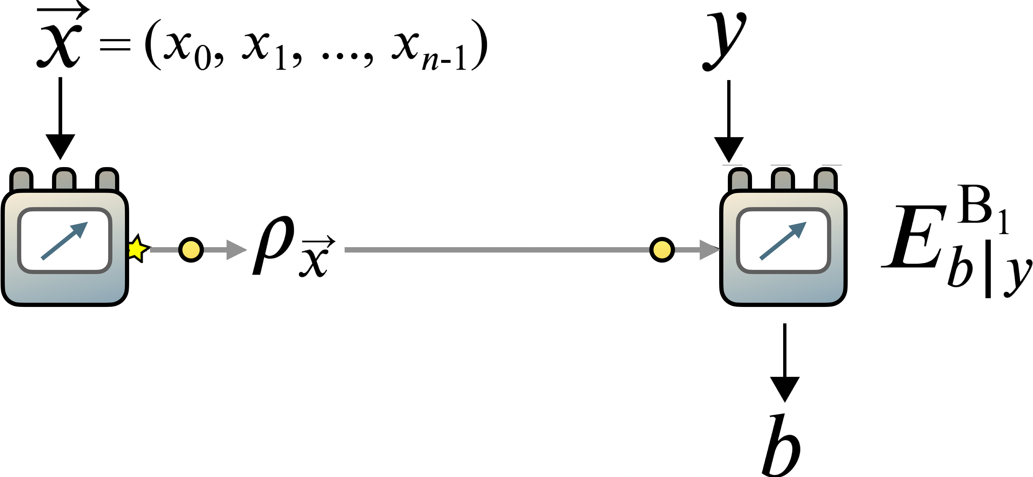
Figure 2: The $n\rightarrow 1$ quantum randomness access codes (QRACs).

For the $3\rightarrow 1$ scenario, there are eight prepared states $\rho_{x_{0},x_{1},x_{2}}$ with $x_{i}\in\{0,1\}$. The correspondence with general temporal scenario can be made by choosing $a^{\prime}=x_{0}$, $x^{\prime}=(x_{1},x_{2})$, $b^{\prime}=b\in\{0,1\}$, and $y^{\prime}=y\in\{0,1,2\}$. The average successful probability is defined as $\mathcal{P}_{3\rightarrow 1}:=\frac{1}{24}\sum_{x_{0},x_{1},x_{2},y}P(b=x_{y}|x_{0},x_{1},x_{2},y)$. Similarly with Eq. (8), an quantum upper bound on $\mathcal{P}_{3\rightarrow 1}$ can be computed. The result matches $\mathcal{P}_{3\rightarrow 1}^{\rm Q}:=\frac{1}{2}(1+1/\sqrt{3})$ for the first level of hierarchy, therefore the bound is tight as well.

Self-testing quantum states in a prepare-and-measure scenario. Finally, we show that the IMMs can be used for verifying set of quantum states in a semi-DI way. More explicitly, we consider the QRAC scenario in the last section and uniquely (up to some isometries) identify the underlying set of states $\rho_{\vec{x}}$ by the observed probabilities $P(b|\vec{x},y)$ only. Such identification, called self-testing in a prepare-and-measure scenario, has been proposed in Refs. Tavakoli et al. (2018); Wei et al. (2019); Miklin and Oszmaniec (2021). We here provide an alternative approach to achieve the task. A robust self-testing of quantum states can be defined as follows Tavakoli et al. (2018); Šupić and Bowles (2020)). Given an upper bound $d$ on the dimension of the systems involved, we say that the observed correlation $\vec{P}:=\{P(b|\vec{x},y)\}_{b,\vec{x},y}$ robustly self-tests, in a prepare-and-measure scenario, the reference set of states $\vec{\rho}_{\rm ref}:=\{\rho_{\vec{x}}^{\rm ref}\}_{\vec{x}}$ at least with a fidelity $f$ if for each set of states $\vec{\rho}:=\{\rho_{\vec{x}}\in\mathcal{H}_{d}\}_{\vec{x}}$ compatible with $\vec{P}$ there exists a completely positive and trace-preserving (CPTP) map $\Lambda$, such that $F(\vec{\rho}_{\rm ref},\Lambda(\vec{\rho}))\geq f$. Here, $\Lambda(\vec{\rho})$ represents for $\Lambda(\rho_{\vec{x}})$ for all $\vec{x}$ and $F(\vec{\rho},\vec{\sigma})$ is the fidelity between two sets of states $\vec{\rho}$ and $\vec{\sigma}$, namely Liang et al. (2019),

$$F(\vec{\rho},\vec{\sigma}):=\sum_{\vec{x}}F^{\rm UJ}(\rho_{\vec{x}},\sigma_{\vec{x}})=\frac{1}{2^{n}}\sum_{\vec{x}}\operatorname{tr}(\rho_{\vec{x}}\sigma_{\vec{x}}),$$ (9)

where $F^{\rm UJ}$ is the Uhlmann-Josza fidelity Uhlmann (1976); Jozsa (1994) and the second equality holds when $\rho_{\vec{x}}$ or $\sigma_{\vec{x}}$ are pure.

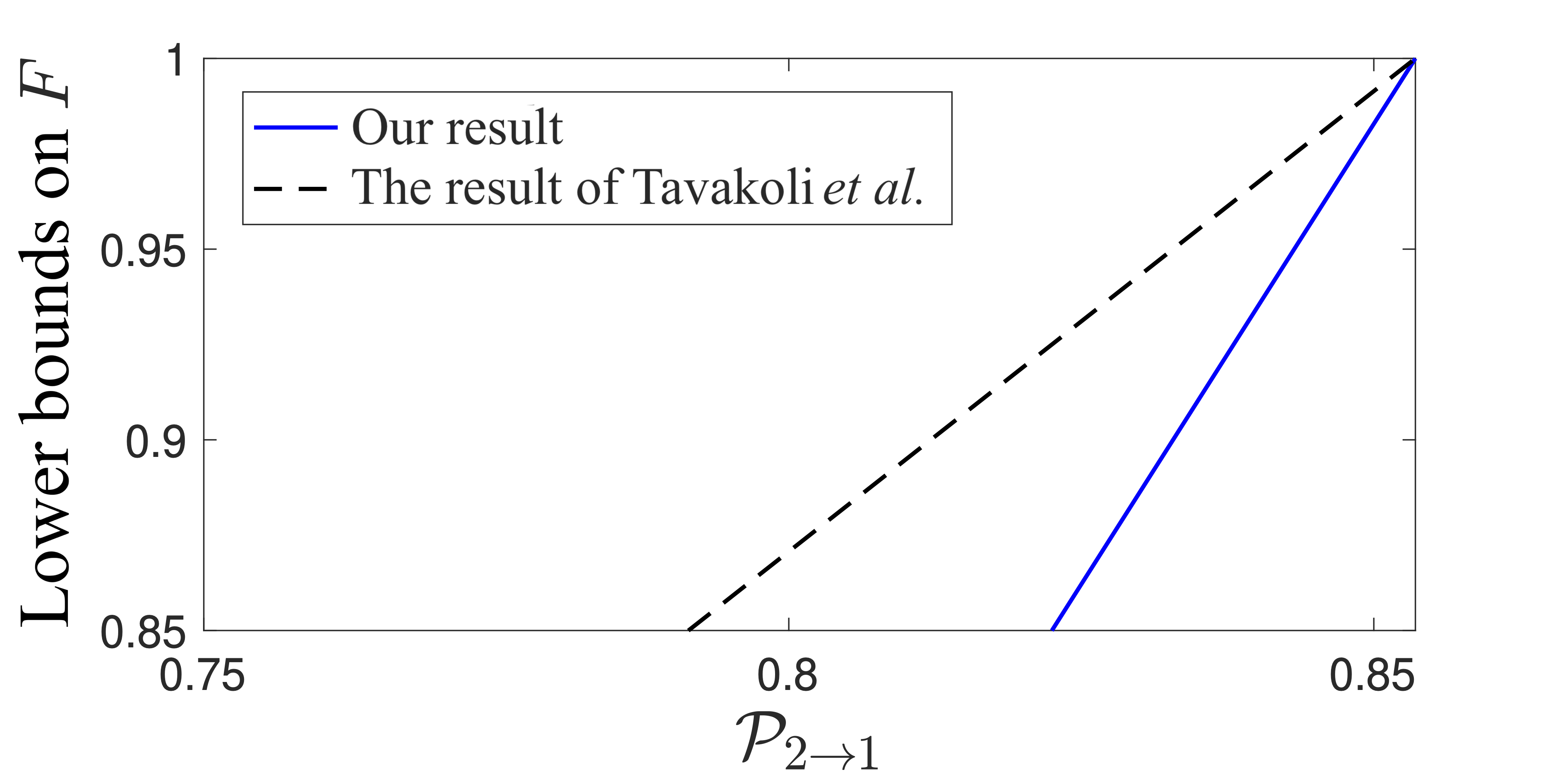
Figure 3: Robust self-testing the reference set of states in the prepare-and-measure scenario.

To compute $F(\vec{\rho}_{\rm ref},\Lambda(\vec{\rho}))$ in a DI way, we use a method similar to that of Ref. Chen et al. (2021b), where the authors self-test steering assemblages. Correcting a flaw in the method of Ref. Chen et al. (2021b) and building on insights of a corrected method Lien and Chen (2023), here, we compute bounds on the fidelity (see Appendix C). The idea is to express the Choi-Jamiołkowski (CJ) matrix reflecting the channel in terms of Bob’s observables. The fidelity can then be written as a polynomial where each monomial is of the form $\operatorname{tr}(\rho_{\vec{x}}S_{j}^{\dagger}S_{i})$ with $S_{i}$ being Bob’s observables or their products. Given the observed correlation $\vec{P}$, a DI bound on $F(\vec{\rho}_{\rm ref},\Lambda(\vec{\rho}))$, denoted as $F^{\rm DI}$, can be computed as

$$\min\bigl{\{}F^{\rm DI}(\vec{\rho}_{\rm ref},\Lambda(\vec{\rho}))\Big{|}\chi_{\vec{x}}\succeq 0,\quad\chi_{\vec{x}}\in\mathcal{G}_{d}^{k}\bigr{\}}.$$ (10)

We consider the example of a $2\to 1$ scenario, where the reference preparation is chosen as a unitary equivalent to $\{|0\rangle,|1\rangle,|+\rangle,|-\rangle\}$, implying $d=2$. We assume the measurement to be projective (as most works do), so that $k=1$. The result is presented by the blue-solid line in Fig. 3. The observed correlation $\vec{P}$ is represented by the average successful probability $\mathcal{P}_{2\rightarrow 1}:=\frac{1}{8}\sum_{x_{0},x_{1},y}P(b=x_{y}|x_{0},x_{1},y)$. Given the maximal quantum value of $\mathcal{P}_{2\rightarrow 1}=\mathcal{P}_{2\rightarrow 1}^{Q}$, we perfectly self-test the reference set of states with fidelity equal to $1$. When $\mathcal{P}_{2\rightarrow 1}$ is below around $0.8232$, we no longer have self-testing statement, since the fidelity is below the classical fidelity $0.8536$ (see Appendix D) The optimal bounds on the fidelity have been proposed in Ref. Tavakoli et al. (2018), i.e., the black-dashed line in Fig. 3. It is an open question how to find the best expression of the CJ matrix to make our bounds optimal.

Summary and discussion. In this work, we have established a general temporal scenario and develop a method, dubbed as instrument moment matrices (IMMs), to characterize quantum temporal correlations generated by such a scenario. The method of IMMs can be implemented in a fully DI scenario, but we can also include additional constraints (such as the dimension and rank of the system) when these information is accessible. Along the side, we contribute to advocating to explore the “room in the middle” between the (precise, but very restrictive) DI and device-specific scenarios: In contrast to Ref. Roth et al. (2023) which is close to device-dependence and is hence dubbed semi-device-dependent, we are here close to the DI regime, in the semi-device-independent setting. We explicitly provide several DI and semi-DI examples, including bounding the maximal value of temporal Bell inequalities and the minimum degree of temporal steerability. Moreover, its variant allows us to compute the maximal successful probability and certify the set of quantum states in a QRAC scenario.

Our work invites a number of questions for future research: First, the temporal scenario considered in this work is composed of two moments of time. There will be more significant applications in the field of quantum network if the framework can be generalized to multiple moments of time. Second, since the construction of the IMMs includes the measurements and channels, we expect that the method of IMMs can be used for certifying properties of quantum measurements and channels, e.g., incompatible measurements or non entanglement-breaking channels, or, even self-testing measurements and channels. Finally, it is interesting to see if the IMMs can also be used for self-testing a set of complex-valued states.

Acknowledgements. We thank Nikolai Miklin, Costantino Budroni, Yeong-Cherng Liang, and Armin Tavakoli for fruitful discussions. S.-L. C. acknowledges the support of the National Science and Technology Council (NSTC) Taiwan (Grant No. NSTC 111-2112-M-005-007-MY4) and National Center for Theoretical Sciences Taiwan (Grant No. NSTC 112-2124-M-002-003). J. E. acknowledges support by the BMBF (QR.X), the Munich Quantum Valley (K-8), and the Einstein Foundation.

Appendix A An example of the IMMs

In this section, we explicitly present an example of IMMs for dichotomic measurement settings and outcomes. For the $1$st level of semi-definite hierarchy, IMMs are $3\times 3$ matrices FN (2)

$$\chi_{a|x}=\begin{pmatrix}\operatorname{tr}[\mathcal{I}_{a|x}(\rho)]&\operatorname{tr}[\mathcal{I}_{a|x}(\rho)E_{0|0}^{\dagger}]&\operatorname{tr}[\mathcal{I}_{a|x}(\rho)E_{0|1}^{\dagger}]\\ \operatorname{tr}[\mathcal{I}_{a|x}(\rho)E_{0|0}]&\operatorname{tr}[\mathcal{I}_{a|x}(\rho)E_{0|0}^{\dagger}E_{0|0}]&\operatorname{tr}[\mathcal{I}_{a|x}(\rho)E_{0|1}^{\dagger}E_{0|0}]\\ \operatorname{tr}[\mathcal{I}_{a|x}(\rho)E_{0|1}]&\operatorname{tr}[\mathcal{I}_{a|x}(\rho)E_{0|0}^{\dagger}E_{0|1}]&\operatorname{tr}[\mathcal{I}_{a|x}(\rho)E_{0|1}^{\dagger}E_{0|1}]\end{pmatrix}.$$ (11)

In a DI setting, $\mathcal{I}_{a|x}^{{\rm A}_{1}\rightarrow{\rm B}_{1}}$, $\rho^{{\rm A}_{1}}$, and $E_{b|y}^{{\rm B}_{1}}$ are unknown. However, we are still able to access some information about $\chi_{a|x}$. For instance, entries corresponding to $\operatorname{tr}[\mathcal{I}_{a|x}(\rho)E_{b|y}]$ are $P(a,b|x,y)$, which are accessible in a DI scheme. Besides, since every POVM can be obtained from a projective measurement with a higher dimension Peres (1990), we can treat $\{E_{b|y}^{{\rm B}_{1}}\}$ as projective measurements, i.e., $E_{b|y}^{{\rm B}_{1}}E_{b^{\prime}|y}^{{\rm B}_{1}}=\delta_{b,b^{\prime}}E_{b|y}^{{\rm B}_{1}}$. Thus $\chi_{a|x}$, can be written as

$$\chi_{a|x}=\begin{pmatrix}P(a|x)&P(a,0|x,0)&P(a,0|x,1)\\ P(a,0|x,0)&P(a,0|x,0)&\operatorname{tr}[\mathcal{I}_{a|x}(\rho)E_{0|1}^{\dagger}E_{0|0}]\\ P(a,0|x,1)&\operatorname{tr}[\mathcal{I}_{a|x}(\rho)E_{0|0}^{\dagger}E_{0|1}]&P(a,0|x,1)\end{pmatrix}.$$ (12)

Entries such as $\operatorname{tr}[\mathcal{I}_{a|x}(\rho)E_{0|1}^{\dagger}E_{0|0}]$ are not accessible in a DI scenario, therefore, they are some unknown complex numbers, denoted by $u_{v}$.

Appendix B Results on the quantification of temporal steerability in DI, DI+Dim., DI+Dim.+Rank, and NSIT scenarios

In the main text, the temporal steering robustness has been computed from the SDP as specified in Eq. (7) as

$$R_{\rm ts}=\min_{\tilde{\sigma}_{\lambda}\succeq 0}~{}\operatorname{tr}\sum_{\lambda}\tilde{\sigma}_{\lambda}-1,$$ (13)

$$\quad{\rm subject~{}to}\quad\sum_{\lambda}\delta_{a,\lambda(x)}\tilde{\sigma}_{\lambda}-\mathcal{I}_{a|x}(\rho)\succeq 0.$$

A common tool to identify bounds is to make use of convex relaxations that give rise to convex outer approximations of the feasible set in optimization problems. Such ideas of semi-definite relaxations have first been used in the context of quantum information science in Refs. Doherty et al. (2004); Eisert et al. (2004). As stated in the main text, by applying the IMMs on the above SDP, the new SDP features relaxed constraints,

$$\min \sum_{\lambda}\mathcal{E}[\sigma_{\lambda}]_{\openone,\openone}-1,$$ (14)

$${\rm subject~{}to} \sum_{\lambda}\delta_{a,\lambda(x)}\mathcal{E}[\tilde{\sigma}_{\lambda}]-\mathcal{E}[\mathcal{I}_{a|x}(\rho)]\succeq 0,$$

$$\mathcal{E}[\tilde{\sigma}_{\lambda}]\succeq 0,\quad\mathcal{E}[\mathcal{I}_{a|x}(\rho)]\succeq 0,$$

$$P(a,b|x,y)=P_{\rm obs}(a,b|x,y),$$

where $\mathcal{E}[\sigma_{\lambda}]_{\openone,\openone}$ represents for $\operatorname{tr}(\sigma_{\lambda}S_{j}^{\dagger}S_{i})$ with $i,j$ being the indices for $S_{i}=S_{j}^{\dagger}=\openone$. The solution of the above SDP is a DI lower bound on $R_{\rm ts}$. For the DI+Dim. result, the dimensional constraint is included in the above SDP of the form

$$\{\mathcal{E}[\mathcal{I}_{a|x}(\rho)]\}_{a,x}\in\mathcal{G}_{d}.$$ (15)

For the DI+Dim.+Rank result, the additional rank constraint is included and the above equation is replaced by

$$\{\mathcal{E}[\mathcal{I}_{a|x}(\rho)]\}_{a,x}\in\mathcal{G}_{d}^{k}.$$ (16)

For the NSIT result, the above constraint is replaced by

$$\sum_{a}\mathcal{E}[\mathcal{I}_{a|x}(\rho)]=\sum_{a}\mathcal{E}[\mathcal{I}_{a|x^{\prime}}(\rho)]\quad\forall x\neq x^{\prime}.$$ (17)

The results are shown in Fig. 4.

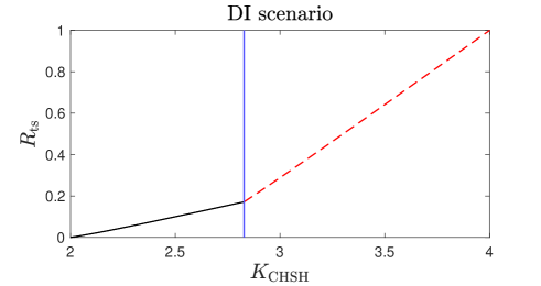
(a)

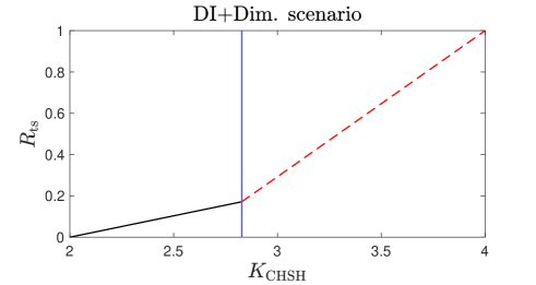
(b)

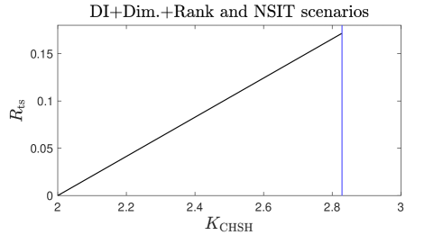
(c)

Figure 4: Given an observed quantum violation of the temporal CHSH value $K_{\rm CHSH}$, we estimate the minimal temporal steering robustness $R_{\rm ts}$ required to achieve the current value $K_{\rm CHSH}$. (a) As can be seen in the figure, in the DI scenario, the bounds can be divided into two ranges of parameters: $2\leq K_{\rm CHSH}\leq 2\sqrt{2}$ and $2\sqrt{2}\leq K_{\rm CHSH}\leq 4$. The former is depicted in the black-solid curve, signifying a noticeable gap (of the order of $10^{-3}$) with a straight line when the IMMs’ level of the hierarchy achieves $5$. The latter is depicted in the red-dashed curve, converging to the straight line described by $R_{\rm ts}=(K_{\rm CHSH}-2)(\sqrt{2}-1)/2$ when the IMMs’ level of the hierarchy achieves $5$. (b) The result of the DI+Dim. scenario is similar to the DI result. The difference is that the bounds converge to linearity, within the numerical precision, in both ranges of $2\leq K_{\rm CHSH}\leq 2\sqrt{2}$ ($1$st level of the IMMs) and $2\sqrt{2}\leq K_{\rm CHSH}\leq 4$ ($4$th level of the IMMs). (c) The lower bounds on $R_{\rm ts}$ computed in the DI+Dim.+Rank and NSIT scenarios both match the straight line $R_{\rm ts}=(K_{\rm CHSH}-2)(\sqrt{2}-1)/2$ within the numerical precision. The vertical blue lines in the three figures represent the value $2\sqrt{2}$, which is the maximal quantum violation in the DI+Dim.+Rank and NSIT scenarios.

Appendix C Detailed derivation of the DI expression of the fidelity

In Ref. Chen et al. (2021b), the method of self-testing steerable assemblages has been proposed. Here, we apply their method on notions of self-testing preparation. The first step is to represent the completely positive map $\Lambda$ with the Choi-Jamiołkowski (CJ) matrix $\Omega$. Namely, $\Lambda(\rho_{\vec{x}})=\operatorname{tr}_{\rm A}[\Omega(\rho_{\vec{x}}^{\mathsf{T}}\otimes\openone)]$ or $[\Lambda(\rho_{\vec{x}})]^{\mathsf{T}}=\operatorname{tr}_{\rm A}[(\rho_{\vec{x}}\otimes\openone)\Omega^{\mathsf{T}}]$ with $\Omega:=(\mathsf{id}\otimes\Lambda)|\phi^{+}\rangle\langle\phi^{+}|$, $|\phi^{+}\rangle:=\sum_{i}|i\rangle_{\rm A}\otimes|i\rangle_{{\rm A}^{\prime}}$, and $\mathsf{id}$ being the identity map. The second step is to choose an optimal quantum strategy which leads to the maximum of $P_{n\rightarrow 1}$. In the main text, we consider the $2\rightarrow 1$ scenario, where the reference set of state vectors is composed of

$$|\psi_{0,0}^{\rm ref}\rangle := c|0\rangle+s|1\rangle,$$ (18)

$$|\psi_{1,0}^{\rm ref}\rangle := s|0\rangle+c|1\rangle,$$ (19)

$$|\psi_{0,1}^{\rm ref}\rangle := -c|0\rangle+s|1\rangle,$$ (20)

$$|\psi_{1,1}^{\rm ref}\rangle := s|0\rangle-c|1\rangle,$$ (21)

with $c:=\cos(\pi/8)$ and $s:=\sin(\pi/8)$. This set is unitarily equivalent with the set $\{|0\rangle,|1\rangle,(|0\rangle+|1\rangle)/\sqrt{2},(|0\rangle-|1\rangle)/\sqrt{2}\}$. We choose the former since Bob’s optimal observables are exactly the two Pauli observables: $B_{0}^{\rm ref}=\hat{Z}$ and $B_{1}^{\rm ref}=\hat{X}$. Until this step, the procedures are the same as the method proposed in Ref. Chen et al. (2021b). As mentioned in the main text, there is a flaw during the construction of the CPTP map $\Lambda$ in Ref. Chen et al. (2021b) and we make the correction as follows. Instead of choosing the identity map (which has been used in Ref. Chen et al. (2021b)), here we choose a map $\Lambda$ caused by the swap operation (see Ref. Lien and Chen (2023) for details). Consequently, the associated CJ matrix $\Omega$ is

$$\Omega^{\mathsf{T}} =|0\rangle\langle 0|\otimes|0\rangle\langle 0|+|1\rangle\langle 0|\otimes|0\rangle\langle 1|+|0\rangle\langle 1|\otimes|1\rangle\langle 0|+|1\rangle\langle 1|\otimes|1\rangle\langle 1|$$

$$=\frac{\openone+B_{0}^{\rm ref}}{2}\otimes|0\rangle\langle 0|+\frac{\openone-B_{0}^{\rm ref}}{2}B_{1}\frac{\openone+B_{0}^{\rm ref}}{2}\otimes|0\rangle\langle 1|+\frac{\openone+B_{0}^{\rm ref}}{2}B_{1}\frac{\openone-B_{0}^{\rm ref}}{2}\otimes|1\rangle\langle 0|+\frac{\openone-B_{0}^{\rm ref}}{2}\otimes|1\rangle\langle 1|.$$

Apparently, there are many choices of the expression in the second line. Each choice can be regarded as an instance of CPTP map $\Lambda$. Plugging the above expression into $[\Lambda(\rho_{\vec{x}})]^{\mathsf{T}}=\operatorname{tr}_{\rm A}[(\rho_{\vec{x}}\otimes\openone)\Omega^{\mathsf{T}}]$, we have

$${}^{\mathsf{T}}= \operatorname{tr}\left(\rho_{x_{0},x_{1}}\frac{\openone+B_{0}^{\rm ref}}{2}\right)|0\rangle\langle 0|+\operatorname{tr}\left(\rho_{x_{0},x_{1}}\frac{\openone-B_{0}^{\rm ref}}{2}B_{1}^{\rm ref}\frac{\openone+B_{0}^{\rm ref}}{2}\right)|0\rangle\langle 1|$$ (22)

$$+ \operatorname{tr}\left(\rho_{x_{0},x_{1}}\frac{\openone+B_{0}^{\rm ref}}{2}B_{1}^{\rm ref}\frac{\openone-B_{0}^{\rm ref}}{2}\right)|1\rangle\langle 0|+\operatorname{tr}\left(\rho_{x_{0},x_{1}}\frac{\openone-B_{0}^{\rm ref}}{2}\right)|1\rangle\langle 1|.$$

Substituting the observables $B_{0}^{\rm ref}$ and $B_{1}^{\rm ref}$ with the POVMs elements $2E_{0|0}^{\rm ref}-\openone$ and $2E_{0|1}^{\rm ref}-\openone$, respectively, we have

$${}^{\mathsf{T}}= \operatorname{tr}\left(\rho_{x_{0},x_{1}}E_{0|0}^{\rm ref}\right)|0\rangle\langle 0|+\operatorname{tr}\left[\rho_{x_{0},x_{1}}(2E_{0|1}^{\rm ref}E_{0|0}^{\rm ref}-2E_{0|0}^{\rm ref}E_{0|1}^{\rm ref}E_{0|0}^{\rm ref})\right]|0\rangle\langle 1|$$ (23)

$$+ \operatorname{tr}\left[\rho_{x_{0},x_{1}}(2E_{0|0}^{\rm ref}E_{0|1}^{\rm ref}-2E_{0|0}^{\rm ref}E_{0|1}^{\rm ref}E_{0|0}^{\rm ref})\right]|1\rangle\langle 0|+\left[1-\operatorname{tr}(\rho_{x_{0},x_{1}}E_{0|0}^{\rm ref})\right]|1\rangle\langle 1|.$$

Using the definition of the fidelity, we find

$$F(\{\rho_{x_{0},x_{1}}^{\rm ref}\},\{\Lambda(\rho_{x_{0},x_{1}})\})$$ (24)

$$= F(\{[\rho_{x_{0},x_{1}}^{\rm ref}]^{\mathsf{T}}\},\{[\Lambda(\rho_{x_{0},x_{1}})]^{\mathsf{T}}\})$$

$$= \frac{1}{4}\sum_{x_{0},x_{1}}\operatorname{tr}\left(\rho_{x_{0},x_{1}}^{\rm ref}\cdot[\Lambda(\rho_{x_{0},x_{1}})]^{\mathsf{T}}\right)$$

$$= \frac{1}{4}\Big{[}2+(c^{2}-s^{2})\operatorname{tr}(\rho_{0,0}E_{0|0}^{\rm ref})-4cs\operatorname{tr}(\rho_{0,0}E_{0|0}^{\rm ref}E_{0|1}^{\rm ref}E_{0|0}^{\rm ref})+2cs\operatorname{tr}(\rho_{0,0}E_{0|1}^{\rm ref}E_{0|0}^{\rm ref})+2cs\operatorname{tr}(\rho_{0,0}E_{0|0}^{\rm ref}E_{0|1}^{\rm ref})+$$

$$\quad\quad\quad(s^{2}-c^{2})\operatorname{tr}(\rho_{1,0}E_{0|0}^{\rm ref})-4cs\operatorname{tr}(\rho_{1,0}E_{0|0}^{\rm ref}E_{0|1}^{\rm ref}E_{0|0}^{\rm ref})+2cs\operatorname{tr}(\rho_{1,0}E_{0|1}^{\rm ref}E_{0|0}^{\rm ref})+2cs\operatorname{tr}(\rho_{1,0}E_{0|0}^{\rm ref}E_{0|1}^{\rm ref})+$$

$$\quad\quad\quad(c^{2}-s^{2})\operatorname{tr}(\rho_{0,1}E_{0|0}^{\rm ref})+4cs\operatorname{tr}(\rho_{0,1}E_{0|0}^{\rm ref}E_{0|1}^{\rm ref}E_{0|0}^{\rm ref})-2cs\operatorname{tr}(\rho_{0,1}E_{0|1}^{\rm ref}E_{0|0}^{\rm ref})-2cs\operatorname{tr}(\rho_{0,1}E_{0|0}^{\rm ref}E_{0|1}^{\rm ref})+$$

$$\quad\quad\quad(s^{2}-c^{2})\operatorname{tr}(\rho_{1,1}E_{0|0}^{\rm ref})+4cs\operatorname{tr}(\rho_{1,1}E_{0|0}^{\rm ref}E_{0|1}^{\rm ref}E_{0|0}^{\rm ref})-2cs\operatorname{tr}(\rho_{1,1}E_{0|1}^{\rm ref}E_{0|0}^{\rm ref})-2cs\operatorname{tr}(\rho_{1,1}E_{0|0}^{\rm ref}E_{0|1}^{\rm ref})\Big{]}.$$

Finally, relaxing the characterized states $\rho_{x_{0},x_{1}}^{\rm ref}$ and POVMs $E_{b|y}^{\rm ref}$ to unknown ones $\rho_{x_{0},x_{1}}$ and $E_{b|y}$, we have a DI expression of fidelity

$$F^{\rm DI}(\{\rho_{x_{0},x_{1}}^{\rm ref}\},\{\Lambda(\rho_{x_{0},x_{1}})\})$$ (25)

$$= \frac{1}{4}\Big{[}2+(c^{2}-s^{2})P(0|0,0,0)-4cs\operatorname{tr}(\rho_{0,0}E_{0|0}E_{0|1}E_{0|0})+2cs\operatorname{tr}(\rho_{0,0}E_{0|1}E_{0|0})+2cs\operatorname{tr}(\rho_{0,0}E_{0|0}E_{0|1})+$$

$$\quad\quad\quad(s^{2}-c^{2})P(0|1,0,0)-4cs\operatorname{tr}(\rho_{1,0}E_{0|0}E_{0|1}E_{0|0})+2cs\operatorname{tr}(\rho_{1,0}E_{0|1}E_{0|0})+2cs\operatorname{tr}(\rho_{1,0}E_{0|0}E_{0|1})+$$

$$\quad\quad\quad(c^{2}-s^{2})P(0|0,1,0)+4cs\operatorname{tr}(\rho_{0,1}E_{0|0}E_{0|1}E_{0|0})-2cs\operatorname{tr}(\rho_{0,1}E_{0|1}E_{0|0})-2cs\operatorname{tr}(\rho_{0,1}E_{0|0}E_{0|1})+$$

$$\quad\quad\quad(s^{2}-c^{2})P(0|1,1,0)+4cs\operatorname{tr}(\rho_{1,1}E_{0|0}E_{0|1}E_{0|0})-2cs\operatorname{tr}(\rho_{1,1}E_{0|1}E_{0|0})-2cs\operatorname{tr}(\rho_{1,1}E_{0|0}E_{0|1})\Big{]},$$

where $P=P(b|x_{0},x_{1},y)$.

Appendix D Classical fidelity

In this section, we show how to compute the classical fidelity $f_{c}\approx 0.8536$ for the self-testing result plotted in Fig. 3. The idea behind the definition of classical fidelity is straightforward: Given a reference set of state, we search for the best classical set of states that gives the highest fidelity. That is,

$$f_{c}:=\max_{\vec{\rho}_{\rm c}}F(\vec{\rho}_{\rm ref},\vec{\rho}_{\rm c})=\max_{\rho_{\vec{x}}^{\rm c}}\frac{1}{4}\sum_{x_{0},x_{1}}\operatorname{tr}(\rho_{x_{0},x_{1}}^{\rm ref}\rho_{x_{0},x_{1}}^{\rm c}),$$ (26)

where $\vec{\rho}_{\rm c}$ denotes a set of classical set of states. In Ref. Tavakoli et al. (2018), the authors have fairly defined a classical set of states: This is the set of states whose elements are all diagonal states, i.e.,

$$\rho_{\vec{x}}^{\rm c}:=\sum_{i}\alpha_{\vec{x},i}|i\rangle\langle i|~{}~{}\forall\vec{x},\quad{\rm with}~{}~{}\sum_{i}\alpha_{\vec{x},i}=1~{}~{}\forall\vec{x}~{}~{}{\rm and}~{}~{}\alpha_{\vec{x},i}\geq 0~{}~{}\forall\vec{x},i,$$ (27)

where $\{|i\rangle\}$ is an orthonormal basis and $\alpha_{\vec{x},i}$ are some real numbers. With this, Eq. (26) can be computed via the linear program

$$\max_{\{\alpha_{x_{0},x_{1},i}\}}\Big{\{}\frac{1}{4}\sum_{x_{0},x_{1},i}\alpha_{x_{0},x_{1},i}\langle i|\rho_{x_{0},x_{1}}^{\rm ref}|i\rangle\Big{|}\sum_{i}\alpha_{x_{0},x_{1},i}=1~{}~{}\forall x_{0},x_{1}~{}~{}{\rm and}~{}~{}\alpha_{x_{0},x_{1},i}\geq 0~{}~{}\forall x_{0},x_{1},i\Big{\}},$$ (28)

and one can obtain $f_{c}\approx 0.8536$.