Low-rank extended Kalman filtering for online learning of neural networks from streaming data

Abstract

We propose an efficient online approximate Bayesian inference algorithm for estimating the parameters of a nonlinear function from a potentially non-stationary data stream. The method is based on the extended Kalman filter (EKF), but uses a novel low-rank plus diagonal decomposition of the posterior precision matrix, which gives a cost per step which is linear in the number of model parameters. In contrast to methods based on stochastic variational inference, our method is fully deterministic, and does not require step-size tuning. We show experimentally that this results in much faster (more sample efficient) learning, which results in more rapid adaptation to changing distributions, and faster accumulation of reward when used as part of a contextual bandit algorithm.

1 Introduction

Suppose we observe a stream of labeled observations, ${\mathcal{D}}_{t}=\{({\bm{x}}_{t}^{n},{\bm{y}}_{t}^{n})\sim p_{t}({\bm{x}},{\bm{y}}):n=1{:}N_{t}\}$, where ${\bm{x}}_{t}^{n}\in\mathcal{X}=^{D}$, ${\bm{y}}_{t}^{n}\in\mathcal{Y}=^{C}$, and $N_{t}$ is the number of examples at step $t$. (In this paper, we assume $N_{t}=1$, since we are interested in rapid learning from individual data samples.) Our goal is to fit a prediction model ${\bm{y}}_{t}=h({\bm{x}}_{t},{\bm{\theta}})$ in an online fashion, where ${\bm{\theta}}\in^{P}$ are the parameters of the model. (We focus on the case where $h$ is a deep neural network (DNN), although in principle our methods can also be applied to other (differentiable) parametric models.) In particular, we want to recursively estimate the posterior over the parameters

$$p({\bm{\theta}}|{\mathcal{D}}_{1:t})\propto p({\bm{y}}_{t}|{\bm{x}}_{t},{\bm{\theta}})p({\bm{\theta}}|{\mathcal{D}}_{1:t-1})$$ (1)

without having to store all the past data. Here $p({\bm{\theta}}|{\mathcal{D}}_{1:t-1})$ is the posterior belief state from the previous step, and $p({\bm{y}}_{t}|{\bm{x}}_{t},{\bm{\theta}})$ is the likelihood function given by

$$p({\bm{y}}_{t}|{\bm{x}}_{t},{\bm{\theta}}) =\begin{cases}\mathcal{N}({\bm{y}}_{t}|h({\bm{x}}_{t},{\bm{\theta}}),\mathbf{R}_{t})&\mbox{regression}\\ \mathrm{Cat}({\bm{y}}_{t}|h({\bm{x}}_{t},{\bm{\theta}}))&\mbox{classification}\end{cases}$$ (2)

For regression, we assume $h({\bm{x}}_{t},{\bm{\theta}})\in^{C}$ returns the mean of the output, and $\mathbf{R}_{t}=R\mathbf{I}_{C}$ is the observation covariance, which we view as a hyper-parameter. For classification, $h({\bm{x}}_{t},{\bm{\theta}})$ returns a $C$-dimensional vector of class probabilities, which is the mean parameter of the categorical distribution.

In many problem settings (e.g., recommender systems (Huang et al., 2015), robotics (Wołczyk et al., 2021; Lesort et al., 2020), and sensor networks (Ditzler et al., 2015)), the data distribution $p_{t}({\bm{x}},{\bm{y}})$ may change over time (Gomes et al., 2019). Hence we allow the model parameters ${\bm{\theta}}_{t}$ to change over time, according to a simple Gaussian dynamics model:

$$p_{t}({\bm{\theta}}_{t}|{\bm{\theta}}_{t-1}) =\mathcal{N}({\bm{\theta}}_{t}|\gamma_{t}{\bm{\theta}}_{t-1},\mathbf{Q}_{t}).$$ (3)

where we usually take $\mathbf{Q}_{t}=q\mathbf{I}$ and $\gamma_{t}=\gamma$, where $q\geq 0$ and $0\leq\gamma\leq 1$. Using $q>0$ injects some noise at each time step, and ensures that the model does not lose “plasticity”, so it can continue to adapt to changes (cf. Kurle et al., 2020; Ash & Adams, 2020; Dohare et al., 2021), and using $\gamma<1$ ensures the variance of the unconditional stochastic process does not blow up. If we set $q=0$ and $\gamma=1$, this corresponds to a deterministic model in which the parameters do not change, i.e.,

$$p_{t}({\bm{\theta}}_{t}|{\bm{\theta}}_{t-1}) =\delta({\bm{\theta}}_{t}-{\bm{\theta}}_{t-1})$$ (4)

This is a useful special case for when we want to estimate the parameters from a stream of data coming from a static distribution. (In practice we find this approach can also work well for the non-stationary setting.)

Recursively computing eq. 1 corresponds to Bayesian inference (filtering) in a state space model, where the dynamics model in eq. 3 is linear Gaussian, but the observation model in eq. 2 is non-linear and possibly non-Gaussian. Many approximate algorithms have been proposed for this task (see e.g. Sarkka, 2013; Murphy, 2023), but in this paper, we focus on Gaussian approximations to the posterior, $q({\bm{\theta}}_{t}|{\mathcal{D}}_{1:t})=\mathcal{N}({\bm{\theta}}_{t}|\bm{\mu}_{t},\bm{\Sigma}_{t})$, since they strike a good balance between efficiency and expressivity. In particular, we build on the extended Kalman filter (EKF), which linearizes the observation model at each step, and then computes a closed form Gaussian update. The EKF has been used for online training of neural networks in many papers (see e.g., Singhal & Wu, 1989; Watanabe & Tzafestas, 1990; Puskorius & Feldkamp, 1991; Iiguni et al., 1992; Ruck et al., 1992; Haykin, 2001). It can be thought of as an approximate Bayesian inference method, or as a natural gradient method for MAP parameter estimation (Ollivier, 2018), which leverages the posterior covariance as a preconditioning matrix for fast Newton-like updates (Alessandri et al., 2007). The EKF was extended to exponential family likelihoods in (Ollivier, 2018; Tronarp et al., 2018), which is necessary when fitting classification models.

The main drawback of the EKF is that it takes $O(P^{3})$ time per step, where $P=|{\bm{\theta}}_{t}|$ is the number of parameters in the hidden state vector, because we need to invert the posterior covariance matrix. It is possible to derive diagonal approximations to the posterior covariance or precision, by either minimizing $D_{\mathbb{KL}}\left({p({\bm{\theta}}_{t}|{\mathcal{D}}_{1:t})}\mathrel{\|}{q({\bm{\theta}}_{t})}\right)$ or $D_{\mathbb{KL}}\left({q({\bm{\theta}}_{t})}\mathrel{\|}{p({\bm{\theta}}_{t}|{\mathcal{D}}_{1:t})}\right)$, as discussed in (Puskorius & Feldkamp, 1991; Chang et al., 2022; Jones et al., 2023). These methods take $O(P)$ time per step, but can be much less statistically efficient than full-covariance methods, since they ignore joint uncertainty between the parameters. This makes the method slower to learn, and slower to adapt to changes in the data distribution, as we show in section 4.

In this paper, we propose an efficient and deterministic method to recursively minimize $D_{\mathbb{KL}}\left({\mathcal{N}({\bm{\theta}}_{t}|\bm{\mu}_{t},\bm{\Sigma}_{t})}\mathrel{\|}{p({\bm{\theta}}_{t}|{\mathcal{D}}_{1:t})}\right)$, where we assume that the precision matrix is diagonal plus low-rank, $\bm{\Sigma}_{t}^{-1}=\bm{\Upsilon}_{t}+\mathbf{W}_{t}\mathbf{W}_{t}^{\intercal}$, where $\bm{\Upsilon}_{t}$ is diagonal and $\mathbf{W}_{t}\in^{P\times L}$ for some memory limit $L$. The key insight is that, if we linearize the observation model at each step, as in the EKF, we can use the resulting gradient vector or Jacobian as “pseudo-observation(s)” that we append to $\mathbf{W}_{t-1}$, and then we can perform an efficient online SVD approximation to obtain $\mathbf{W}_{t}$. We therefore call our method LO-FI, which is short for low-rank extended Kalman filter. Our code is available at https://github.com/probml/rebayes.

We use the posterior approximation $p({\bm{\theta}}_{t}|{\mathcal{D}}_{1:t})$ in two ways. First, under Bayesian updating the covariance matrix $\bm{\Sigma}_{t}$ acts as a preconditioning matrix to yield a deterministic second-order Newton-like update for the posterior mean (MAP estimate). This update does not have any step-size hyperparameters, in contrast to SGD. Second, the posterior uncertainty in the parameters can be propagated into the uncertainty of the predictive distribution for observations, which is crucial for online decision-making tasks, such as active learning (Holzmüller et al., 2022), Bayesian optimization (Garnett, 2023), contextual bandits (Duran-Martin et al., 2022), and reinforcement learning (Khetarpal et al., 2022; Wang et al., 2021).

In summary, our main contribution is a novel algorithm for efficiently (and deterministically) recursively updating a diagonal plus low-rank (DLR) approximation to the precision matrix of a Gaussian posterior for a special kind of state space model, namely an SSM with an arbitrary non-linear (and possibly non-Gaussian) observation model, but with a simple linear Gaussian dynamics. This model family is ideally suited to online parameter learning for DNNs in potentially non-stationary environments (but the restricted form of the dynamics model excludes some other applications of SSMs). We show experimentally that our approach works better (in terms of accuracy for a given compute budget) than a variety of baseline algorithms — including online gradient descent, online Laplace, diagonal approximations to the EKF, and a stochastic DLR VI method called L-RVGA — on a variety of stationary and non-stationary classification and regression problems, as well as a simple contextual bandit problem.

2 Related work

Since exact Bayesian inference is intractable in our model family, it is natural to compute an approximate posterior at step $t$ using recursive variational inference (VI), in which the prior for step $t$ is the approximate posterior from step $t-1$ (Opper, 1998; Broderick et al., 2013). That is, at each step we minimize the ELBO (evidence lower bound), which is equal (up to a constant) to the reverse KL, given by

$$\mathcal{L}(\bm{\mu}_{t},\bm{\Sigma}_{t})=D_{\mathbb{KL}}\left({\mathcal{N}({\bm{\theta}}_{t}|\bm{\mu}_{t},\bm{\Sigma}_{t})}\mathrel{\|}{Z_{t}p({\bm{y}}_{t}|{\bm{x}}_{t},{\bm{\theta}}_{t})q_{t|t-1}({\bm{\theta}}_{t}|{\mathcal{D}}_{1:t-1})}\right)$$ (5)

where $Z_{t}$ is a normalization constant and $q_{t}=\mathcal{N}({\bm{\theta}}_{t}|\bm{\mu}_{t},\bm{\Sigma}_{t})$ is the variational posterior which results from minimizing this expression. The main challenge is how to efficiently optimize this objective.

One common approach is to assume the variational family consists of a diagonal Gaussian. By linearizing the likelihood, we can solve the VI objective in closed form, as shown in (Chang et al., 2022); this is called the “variational diagonal EKF” (VD-EKF). They also propose a diagonal approximation which minimizes the forwards KL, $D_{\mathbb{KL}}\left({p({\bm{\theta}}_{t}|{\mathcal{D}}_{1:t})}\mathrel{\|}{q({\bm{\theta}}_{t})}\right)$, and show that this is equivalent to the “fully decoupled EKF” (FD-EKF) method of (Puskorius & Feldkamp, 1991). Both of these methods are fully deterministic, which avoids the high variance that often plagues stochastic VI methods (Wu et al., 2019; Haußmann et al., 2020).

It is also possible to derive diagonal approximations without linearizing the observation model. In (Kurle et al., 2020; Zeno et al., 2018) they propose a diagonal approximation to minimize the reverse KL, $D_{\mathbb{KL}}\left({q({\bm{\theta}}_{t})}\mathrel{\|}{p({\bm{\theta}}_{t}|{\mathcal{D}}_{1:t})}\right)$; this requires a Monte Carlo approximation to the ELBO. In (Ghosh et al., 2016; Wagner et al., 2022), they propose a diagonal approximation to minimize the forwards KL, $D_{\mathbb{KL}}\left({p({\bm{\theta}}_{t}|{\mathcal{D}}_{1:t})}\mathrel{\|}{q({\bm{\theta}}_{t})}\right)$; this requires approximating the first and second moments of the hidden units at every layer of the model using numerical integration.

(Farquhar et al., 2020) claims that, if one makes the model deep enough, one can get good performance using a diagonal approximation; however, this has not been our experience. This motivates the need to go beyond a diagonal approximation.

One approach is to combine diagonal Gaussian approximations with memory buffers, such as the variational continual learning methd of (Nguyen et al., 2018) and other works (see e.g., (Kurle et al., 2020; Khan & Swaroop, 2021)). However, we seek to find a richer approximation to the posterior that does not rely on memory buffers, which can be problematic in the non-stationary setting.

(Zeno et al., 2021) proposes the FOO-VB method, which uses a Kronecker block structured approximation to the posterior covariance. However, this method requires 2 SVD decompositions of the Kronecker factors for every layer of the model, in addition to a large number of Monte Carlo samples, at each time step. In (Ong et al., 2018) they compute a diagonal plus low-rank (DLR) approximation to the posterior covariance matrix using stochastic gradient applied to the ELBO. In (Tomczak et al., 2020) they develop a version of the local reparameterization trick for the DLR posterior covariance, to reduce the variance of the stochastic gradient estimate.

In this paper we use a diagonal plus low-rank (DLR) approximation to the posterior precision. The same form of approximation has been used in several prior papers. In (Mishkin et al., 2018) they propose a technique called “SLANG” (stochastic low-rank approximate natural-gradient), which uses a stochastic estimate of the natural gradient of the ELBO to update the posterior precision, combined with a randomized eigenvalue solver to compute a DLR approximation. Their NGD approximation enables the variational updates to be calculated solely from the loss gradients, whereas our approach requires the network Jacobian. On the other hand, our EKF approach allows the posterior precision and the DLR approximation to be efficiently computed in closed form.

In (Lambert et al., 2021a), they propose a technique called “L-RVGA” (low-rank recursive variational Gaussian approximation), which uses stochastic EM to optimize the ELBO using a DLR approximation to the posterior precision. Their method is a one-pass online method, like ours, and also avoids the need to tune the learning rate. However, it is much slower, since it involves generating multiple samples from the posterior and multiple iterations of the EM algorithm (see fig. 7 for an experimental comparison of running time).

The GGT method of (Agarwal et al., 2019) also computes a DLR approximation to the posterior precision, which they use as a preconditioner for computing the MAP estimate. However, they bound the rank by simply using the most recent $L$ observations, whereas LO-FI uses SVD to combine the past data in a more efficient way.

The ORFit method of (Min et al., 2022) is also an online low-rank MAP estimation method. They use orthogonal projection to efficiently compute a low rank representation of the precision at each step. However, it is restricted to regression problems with 1d, noiseless outputs (i.e., they assume the likelihood has the degenerate form $p(y_{t}|{\bm{x}}_{t},{\bm{\theta}}_{t})=\mathcal{N}(h({\bm{x}}_{t},{\bm{\theta}}_{t}),0)$.)

The online Laplace method of (Ritter et al., 2018; Daxberger et al., 2021) also computes a Gaussian approximation to the posterior, but makes different approximations. In particular, for “task” $t$, it computes the MAP estimate ${\bm{\theta}}_{t}=\operatornamewithlimits{argmax}_{{\bm{\theta}}}\log p({\mathcal{D}}_{t}|{\bm{\theta}})+\log\mathcal{N}({\bm{\theta}}|\bm{\mu}_{t-1},\bm{\Sigma}_{t-1})$, where $\bm{\Sigma}_{t-1}=\bm{\Lambda}_{t-1}^{-1}$ is the approximate posterior covariance from the previous task. (This optimization problem is solved using SGD applied to a replay buffer.) This precision matrix is usually approximated as a block diagonal matrix, with one block per layer, and the terms within each block may be additionally approximated by a Kronecker product form, as in KFAC (Martens & Grosse, 2015). By contrast, LO-FI computes a posterior, not just a point estimate, and approximates the precision as diagonal plus low rank. In the appendix, we show experimentally that LO-FI outperforms online Laplace in terms of NLPD on various classification and regression tasks.

It is possible to go beyond Gaussian approximations by using particle filtering (see e.g., (Yang et al., 2023)). However, we focus on faster deterministic inference methods, since speed is important for many real time online decision making tasks (Ghunaim et al., 2023).

There are many papers on continual learning, which is related to online learning. However the CL literature usually assumes the task boundaries, corresponding to times when the distribution shifts, are given to the learner (see e.g., (Delange et al., 2021; De Lange & Tuytelaars, 2021; Wang et al., 2022; Mai et al., 2022; Mundt et al., 2023; Wang et al., 2023).) By contrast, we are interested in the continual learning setting where the distribution may change at unknown times, in a continuous or discontinuous manner (c.f., (Gama et al., 2013)); this is sometimes called the “task agnostic” or “streaming” setting. Furthermore, our goal is accurate forecasting of the future (which can be approximated by our estimate of the “current” distribution), so we are less concerned with performance on “past” distributions that the agent may not encounter again; thus “catastrophic forgetting” (see e.g., (Parisi et al., 2019)) is not a focus of this work (c.f., (Dohare et al., 2021)).

3 Methods

In LO-FI, we approximate the belief state by a Gaussian, $p({\bm{\theta}}_{t}|{\mathcal{D}}_{1:t})=\mathcal{N}(\bm{\mu}_{t},\bm{\Sigma}_{t})$, where the posterior precision is diagonal plus low rank, i.e., it has the form $\bm{\Sigma}_{t}^{-1}=\bm{\Upsilon}_{t}+\mathbf{W}_{t}\mathbf{W}_{t}^{\mkern-1.5mu\mathsf{T}}$, where $\bm{\Upsilon}_{t}$ is diagonal and $\mathbf{W}_{t}$ is a $P\times L$ matrix. We denote this class of models by $\text{DLR}(L)$, where $L$ is the rank. Below we show how to efficiently update this belief state in a recursive (online) fashion. This has two main steps — predict (see algorithm 2) and update (see algorithm 3) — which are called repeatedly, as shown in algorithm 1. The predict step takes $O(PL^{2}+L^{3})$ time, and the update step takes $O(P(L+C)^{2})$ time, where $C$ is the number of outputs.

1def $\text{lofi}(\bm{\mu}_{0},\bm{\Upsilon}_{0},{\bm{x}}_{1:T},{\bm{y}}_{1:T},\gamma_{1:T},q_{1:T},L,h)$

2 $\mathbf{W}_{0}=\bm{0}$

3 foreach $t=1:T$ do

4       $(\bm{\mu}_{t|t-1},\bm{\Upsilon}_{t|t-1},\mathbf{W}_{t|t-1},\hat{{\bm{y}}}_{t})=\text{predict}(\bm{\mu}_{t-1},\bm{\Upsilon}_{t-1},\mathbf{W}_{t-1},{\bm{x}}_{t},\gamma_{t},q_{t},h)$

5       $(\bm{\mu}_{t},\bm{\Upsilon}_{t},\mathbf{W}_{t})=\text{update}(\bm{\mu}_{t|t-1},\bm{\Upsilon}_{t|t-1},\mathbf{W}_{t|t-1},{\bm{x}}_{t},{\bm{y}}_{t},\hat{{\bm{y}}}_{t},h,L)$

6       $\text{callback}(\hat{{\bm{y}}}_{t},{\bm{y}}_{t})$

Algorithm 1 LOFI main loop.

3.1 Predict step

1def $\text{predict}(\bm{\mu}_{t-1},\bm{\Upsilon}_{t-1},\mathbf{W}_{t-1},{\bm{x}}_{t},\gamma_{t},q_{t},h)$:

2 $\bm{\mu}_{t|t-1}=\gamma_{t}\bm{\mu}_{t-1}$ // Predict the mean of the next state

3 $\bm{\Upsilon}_{t|t-1}=\left(\gamma_{t}^{2}\bm{\Upsilon}_{t-1}^{-1}+q_{t}\mathbf{I}_{P}\right)^{-1}$ // Predict the diagonal precision

4 $\mathbf{C}_{t}=\left(\mathbf{I}_{L}+q_{t}\mathbf{W}_{t-1}^{{\mkern-1.5mu\mathsf{T}}}\bm{\Upsilon}_{t|t-1}\bm{\Upsilon}_{t-1}^{-1}\mathbf{W}_{t-1}\right)^{-1}$

5 $\mathbf{W}_{t|t-1}=\gamma_{t}\bm{\Upsilon}_{t|t-1}\bm{\Upsilon}_{t-1}^{-1}\mathbf{W}_{t-1}{\rm chol}(\mathbf{C}_{t})$ // Predict the low-rank precision

6 $\hat{{\bm{y}}}_{t}=h\left({\bm{x}}_{t},\bm{\mu}_{t|t-1}\right)$ // Predict the mean of the output

Return $(\bm{\mu}_{t|t-1},\bm{\Upsilon}_{t|t-1},\mathbf{W}_{t|t-1},\hat{{\bm{y}}}_{t})$

Algorithm 2 LO-FI predict step.

In the predict step, we go from the previous posterior, $p({\bm{\theta}}_{t-1}|{\mathcal{D}}_{1:t-1})=\mathcal{N}({\bm{\theta}}_{t-1}|\bm{\mu}_{t-1},\bm{\Sigma}_{t-1})$, to the one-step-ahead predictive distribution, $p({\bm{\theta}}_{t}|{\mathcal{D}}_{1:t-1})=\mathcal{N}({\bm{\theta}}_{t}|\bm{\mu}_{t|t-1},\bm{\Sigma}_{t|t-1})$. To compute this predictive distribution, we apply the dynamics in eq. 3 with $\mathbf{Q}_{t}=q_{t}\mathbf{I}$ to get $\bm{\mu}_{t|t-1}=\gamma_{t}\bm{\mu}_{t-1}$ and $\bm{\Sigma}_{t|t-1}=\gamma_{t}^{2}\bm{\Sigma}_{t-1}+q_{t}\mathbf{I}_{P}$. However, this recursion is in terms of the covariance matrix, but we need the corresponding result for a DLR precision matrix in order to be computationally efficient. In section A.1 we show how to use the matrix inversion lemma to efficiently compute $\bm{\Sigma}^{-1}_{t|t-1}=\bm{\Upsilon}_{t|t-1}+\mathbf{W}_{t|t-1}\mathbf{W}_{t|t-1}^{\mkern-1.5mu\mathsf{T}}$. The result is shown in the pseudocode in algorithm 2, where $\mathbf{A}={\rm chol}(\mathbf{B})$ denotes Cholesky decomposition (i.e., $\mathbf{A}\mathbf{A}^{\mkern-1.5mu\mathsf{T}}=\mathbf{B}$). The cost of computing $\bm{\Upsilon}_{t|t-1}$ is $O(P)$ since it is diagonal. The cost of computing $\mathbf{W}_{t|t-1}$ is $O(PL^{2}+L^{3})$. If we use a full-rank approximation, $L=P$, we recover the standard EKF predict step.

3.2 Update step

1def $\text{update}(\bm{\mu}_{t|t-1},\bm{\Upsilon}_{t|t-1},\mathbf{W}_{t|t-1},{\bm{x}}_{t},{\bm{y}}_{t},\hat{{\bm{y}}}_{t},h,L)$:

2 $\mathbf{R}_{t}=h_{V}({\bm{x}}_{t},\bm{\mu}_{t|t-1})$ // Covariance of predicted output

3 $\mathbf{L}_{t}=\text{chol}(\mathbf{R}_{t})$

4 $\mathbf{A}_{t}=\mathbf{L}_{t}^{-1}$

5 $\mathbf{H}_{t}=\text{jac}(h({\bm{x}}_{t},\cdot))(\bm{\mu}_{t|t-1})$ // Jacobian of observation model

6 $\tilde{\mathbf{W}}_{t}=\left[\begin{array}[]{cc}\mathbf{W}_{t|t-1}&\mathbf{H}_{t}^{{\mkern-1.5mu\mathsf{T}}}\mathbf{A}_{t}^{\mkern-1.5mu\mathsf{T}}\end{array}\right]$ // Expand low-rank with new observation

7 $\mathbf{G}_{t}=\left(\mathbf{I}_{\tilde{L}}+\tilde{\mathbf{W}}_{t}^{{\mkern-1.5mu\mathsf{T}}}\bm{\Upsilon}_{t|t-1}^{-1}\tilde{\mathbf{W}}_{t}\right)^{-1}$

8 $\mathbf{C}_{t}=\mathbf{H}_{t}^{{\mkern-1.5mu\mathsf{T}}}\mathbf{A}_{t}^{\mkern-1.5mu\mathsf{T}}\mathbf{A}_{t}$

9 $\mathbf{K}_{t}=\bm{\Upsilon}_{t|t-1}^{-1}\mathbf{C}_{t}-\bm{\Upsilon}_{t|t-1}^{-1}\tilde{\mathbf{W}}_{t}\mathbf{G}_{t}\tilde{\mathbf{W}}_{t}^{{\mkern-1.5mu\mathsf{T}}}\bm{\Upsilon}_{t|t-1}^{-1}\mathbf{C}_{t}$ // Kalman gain matrix

10 $\bm{\mu}_{t}=\bm{\mu}_{t|t-1}+\mathbf{K}_{t}({\bm{y}}_{t}-\hat{{\bm{y}}}_{t})$ // Mean update

11 $(\tilde{\bm{\Lambda}}_{t},\tilde{\mathbf{U}}_{t})={\rm SVD}(\tilde{\mathbf{W}}_{t})$ // Take SVD of the expanded low-rank

12 $(\bm{\Lambda}_{t},\mathbf{U}_{t})=\left(\tilde{\bm{\Lambda}}_{t},\tilde{\mathbf{U}}_{t}\right)[:,1{:}L]$ // Keep top $L$ most important terms

13 $\mathbf{W}_{t}=\mathbf{U}_{t}\bm{\Lambda}_{t}$ // New low-rank approximation

14 $(\bm{\Lambda}_{t}^{\times},\mathbf{U}_{t}^{\times})=\left(\tilde{\bm{\Lambda}}_{t},\tilde{\mathbf{U}}_{t}\right)[:,(L+1){:}\tilde{L}]$ // Extract remaining least important terms

15 $\mathbf{W}_{t}^{\times}=\mathbf{U}_{t}^{\times}\bm{\Lambda}_{t}^{\times}$ // The low-rank part that is dropped

16 $\bm{\Upsilon}_{t}=\bm{\Upsilon}_{t|t-1}+\mathrm{diag}\left(\mathbf{W}_{t}^{\times}(\mathbf{W}_{t}^{\times})^{{\mkern-1.5mu\mathsf{T}}}\right)$ // Update diagonal to capture variance due to dropped terms

Return $(\bm{\mu}_{t},\bm{\Upsilon}_{t},\mathbf{W}_{t})$

Algorithm 3 LO-FI update step.

In the update step, we go from the prior predictive distribution, $p({\bm{\theta}}_{t}|{\mathcal{D}}_{1:t-1})=\mathcal{N}({\bm{\theta}}_{t}|\bm{\mu}_{t|t-1},\bm{\Sigma}_{t|t-1})$, to the posterior distribution, $p({\bm{\theta}}_{t}|{\mathcal{D}}_{1:t})=\mathcal{N}({\bm{\theta}}_{t}|\bm{\mu}_{t},\bm{\Sigma}_{t})$. Unlike the predict step, this cannot be computed exactly. Instead we will compute an approximate posterior $q_{t}$ by minimizing the KL objective in eq. 5. One can show (see e.g., Opper & Archambeau, 2009; Kurle et al., 2020; Lambert et al., 2021b) that the optimum must satisfy the following fixed-point equations:

$$\bm{\mu}_{t} =\bm{\mu}_{t|t-1}+\bm{\Sigma}_{t-1}\nabla_{\bm{\mu}_{t}}\mathbb{E}_{{q_{t}}}\left[{\log p({\bm{y}}_{t}|{\bm{\theta}}_{t})}\right]=\bm{\mu}_{t|t-1}+\bm{\Sigma}_{t-1}\mathbb{E}_{{q_{t}}}\left[{\nabla_{{\bm{\theta}}_{t}}\log p({\bm{y}}_{t}|{\bm{\theta}}_{t})}\right]$$ (6)

$$\bm{\Sigma}_{t}^{-1} =\bm{\Sigma}_{t|t-1}^{-1}-2\nabla_{\bm{\Sigma}_{t}}\mathbb{E}_{{q_{t}}}\left[{\log p({\bm{y}}_{t}|{\bm{\theta}}_{t})}\right]=\bm{\Sigma}_{t|t-1}^{-1}-\mathbb{E}_{{q_{t}}}\left[{\nabla_{{\bm{\theta}}_{t}}^{2}\log p({\bm{y}}_{t}|{\bm{\theta}}_{t})}\right]$$ (7)

Note that this is an implicit equation, since $q_{t}$ occurs on the left and right hand sides. A common approach to solving this optimization problem (e.g., used in (Mishkin et al., 2018; Kurle et al., 2020; Lambert et al., 2021b)) is to approximate the expectation with samples from the prior predictive, $q_{t|t-1}$. In addition, it is common to approximate the Hessian matrix with the generalized Gauss Newton (GGN) matrix, which is derived from the Jacobian, as we explain below. In this paper we replace the Monte Carlo expectations with analytic methods, by leveraging the same GGN approximation. We then generalize to the low-rank setting to make the method efficient.

In more detail, we compute a linear-Gaussian approximation to the likelihood function, after which the KL optimization problem can be solved exactly by performing conjugate Bayesian updating. To approximate the likelihood, we first linearize the observation model about the prior predictive mean:

$$\hat{h}_{t}({\bm{\theta}}_{t})=h({\bm{x}}_{t},\bm{\mu}_{t|t-1})+\mathbf{H}_{t}({\bm{\theta}}_{t}-\bm{\mu}_{t|t-1})$$ (8)

where $\mathbf{H}_{t}$ is the $C\times P$ Jacobian of $h({\bm{x}}_{t},\cdot)$ evaluated at $\bm{\mu}_{t|t-1}$. To handle non-Gaussian outputs, we follow Ollivier (2018) and Tronarp et al. (2018), and approximate the output distribution using a Gaussian, whose conditional moments are given by

$$\hat{{\bm{y}}}_{t} =\mathbb{E}\left[{{\bm{y}}_{t}|{\bm{x}}_{t},{\bm{\theta}}_{t}=\bm{\mu}_{t|t-1}}\right]=h({\bm{x}}_{t},\bm{\mu}_{t|t-1})$$ (9)

$$\mathbf{R}_{t} =\mathrm{Cov}\left[{{\bm{y}}_{t}|{\bm{x}}_{t},{\bm{\theta}}_{t}=\bm{\mu}_{t|t-1}}\right]=h_{V}({\bm{x}}_{t},\bm{\mu}_{t|t-1})=\begin{cases}R_{t}\,\mathbf{I}_{C}&\mbox{regression}\\ \mathrm{diag}(\hat{{\bm{y}}}_{t})-\hat{{\bm{y}}}_{t}\hat{{\bm{y}}}_{t}^{\mkern-1.5mu\mathsf{T}}&\mbox{classification}\end{cases}$$ (10)

where $\hat{{\bm{y}}}_{t}$ is a vector of $C$ probabilities in the case of classification.

Under the above assumptions, we can use the standard EKF update equations (see e.g., Sarkka, 2013). In section A.2 we extend these equations to the case where the precision matrix is DLR; this forms the core of our LO-FI method. The basic idea is to compute the exact update to get $\bm{\Sigma}_{t}^{*-1}=\bm{\Upsilon}_{t}+\tilde{\mathbf{W}}_{t}\tilde{\mathbf{W}}_{t}^{\mkern-1.5mu\mathsf{T}}$, where $\tilde{\mathbf{W}}_{t}$ extends $\mathbf{W}_{t|t-1}$ with $C$ additional columns coming from the Jacobian of the observation model, and then to project $\tilde{\mathbf{W}}_{t}$ back to rank $L$ using SVD to get $\bm{\Sigma}_{t}^{-1}=\bm{\Upsilon}_{t}+\mathbf{W}_{t}\mathbf{W}_{t}^{\mkern-1.5mu\mathsf{T}}$, where $\bm{\Upsilon}_{t}$ is chosen so as to satisfy $\mathrm{diag}(\bm{\Sigma}_{t}^{-1})=\mathrm{diag}(\bm{\Sigma}_{t}^{*-1})$. See algorithm 3 for the resulting pseudocode. The cost is dominated by the $O(P\tilde{L}^{2})$ time needed for the SVD, where $\tilde{L}=L+C$.

To gain some intuition for the method, suppose the output is scalar, with variance $R=1$. Then we have $A_{t}=1$ and $\mathbf{H}_{t}^{\mkern-1.5mu\mathsf{T}}=\nabla_{{\bm{\theta}}_{t}}h({\bm{x}}_{t},{\bm{\theta}}_{t})={\bm{g}}_{t}$ as the approximate linear observation matrix. (Note that, for a linear model, we have ${\bm{g}}_{t}={\bm{x}}_{t}$.) In this case, we have $\tilde{\mathbf{W}}_{t}=\left[\begin{array}[]{cc}\mathbf{W}_{t|t-1}&{\bm{g}}_{t}\end{array}\right]$. Thus $\tilde{\mathbf{W}}_{t}$ acts like a generalized memory buffer that stores data using a gradient embedding. This allows an interpretation of our method in terms of the neural tangent kernel (Jacot et al., 2018), although we leave the details to future work.

3.3 Predicting the observations

So far we have just described how to recursively update the belief state for the parameters. To predict the output ${\bm{y}}_{t}$ given a test input ${\bm{x}}_{t}$, we need to compute the one-step-ahead predictive distribution

$$p({\bm{y}}_{t}|{\bm{x}}_{t},{\mathcal{D}}_{1:t-1}) =\int p({\bm{y}}_{t}|{\bm{x}}_{t},{\bm{\theta}}_{t})p({\bm{\theta}}_{t}|{\mathcal{D}}_{1:t-1})d{\bm{\theta}}_{t}$$ (11)

The negative log of this, $-\log p({\bm{y}}_{t}|{\bm{x}}_{t},{\mathcal{D}}_{1:t-1})$, is called the negative log predictive density or NLPD. If we ignore the posterior uncertainty, this integral gives us the following plugin approximation, given by

$$p({\bm{y}}_{t}|{\bm{x}}_{t},{\mathcal{D}}_{1:t-1}) \approx\int p({\bm{y}}_{t}|{\bm{x}}_{t},{\bm{\theta}}_{t})\mathcal{N}({\bm{\theta}}_{t}|\bm{\mu}_{t|t-1},0\mathbf{I})d{\bm{\theta}}_{t}=p({\bm{y}}_{t}|{\bm{x}}_{t},\bm{\mu}_{t|t-1})$$ (12)

The negative log of this, $-\log p({\bm{y}}_{t}|{\bm{x}}_{t},\bm{\mu}_{t|t-1})$, is called the negative log likelihood or NLL. We report NLL results in the main paper, since they are easy to compute.

However, we can get better performance by using more accurate approximations to the integral. The simplest approach is to use Monte Carlo sampling; alternatively we can use deterministic approximations, as discussed in appendix B. We find that naively passing posterior samples through the model can result in worse performance than using the plugin approximation, which just uses the posterior mode. However, if we pass the samples through the linearized observation model, as proposed in (Immer et al., 2021), we find that the NLPD can outperform the NLL, as shown in section D.3 and section D.6 in the appendix.

3.4 Initialization and hyper-parameter tuning

The natural way to initialize the belief state is use a vague Gaussian prior of the form $p({\bm{\theta}}_{0})=\mathcal{N}(\bm{0},\bm{\Upsilon}_{0})$, where $\bm{\Upsilon}_{0}=\eta_{0}\mathbf{I}_{P}$ and $\eta_{0}$ is a hyper-parameter that controls the strength of the prior. However, plugging in all 0s for the weights will result in a prediction of 0, which will result in a zero gradient, and so no learning will take place. (With $\bm{\mu}_{0}=0$, no deterministic algorithm can ever break the network’s inherent symmetry under permutation of the hidden units.) So in practice we sample the initial mean weights using a standard neural network initialization procedure, such as “LeCun-Normal”, which has the form $\bm{\mu}_{0}\sim\mathcal{N}(\bm{0},\mathbf{S}_{0})$, where $\mathbf{S}_{0}$ is diagonal and $S_{0}[j,j]=1/F_{j}$ is the fan-in of weight $j$. (The bias terms are initialized to 0.) We then set $\bm{\Upsilon}_{0}=\eta_{0}\mathbf{I}_{P}$ and $\mathbf{W}_{0}=[0]^{P\times L}$.

The hyper-parameters of our method are the initial prior precision $\eta_{0}$, the dynamics noise $q$, the dynamics scaling factor $\gamma$, and (for regression problems), the observation variance $R$. These play a role similar to the hyper-parameters of a standard neural network, such as degree of regularization and the learning rate. We optimize these hyper-parameters using Bayesian optimization, where the objective is the validation set NLL for stationary problems, or the average one-step-ahead NLL (aka prequential loss) for non-stationary problems. For details, see appendix C.

4 Experiments

In this section, we report experimental results on various classification and regression datasets. using the following approximate inference techniques: LO-FI (this paper); FDEKF (fully decoupled diagonal EKF) (Puskorius & Feldkamp, 2003); VDEKF (variational diagonal EKF) (Chang et al., 2022); SGD-RB (stochastic gradient descent with FIFO replay buffer), with memory buffer of size $B$, using either sgd or adam as the optimizer; online gradient descent (OGD), which corresponds to SGD-RB with $B=1$; the LRVGA method of (Lambert et al., 2021a) (for the NLPD results in section D.1); and the online Laplace approximation of (Ritter et al., 2018) (for the NLPD results in section D.3 and section D.6). For additional results, see appendix D. For the source code to reproduce these results, see https://github.com/probml/rebayes.

4.1 Classification

In this section, we report results on various image classification datasets. We use a 2-layer MLP (with 500 hidden units each), which has $648,010$ parameters. (For results using a CNN, see section D.3 in the appendix.)

Stationary distribution

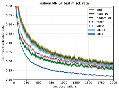
(a)

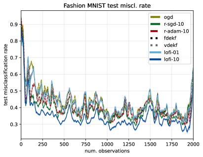
(b)

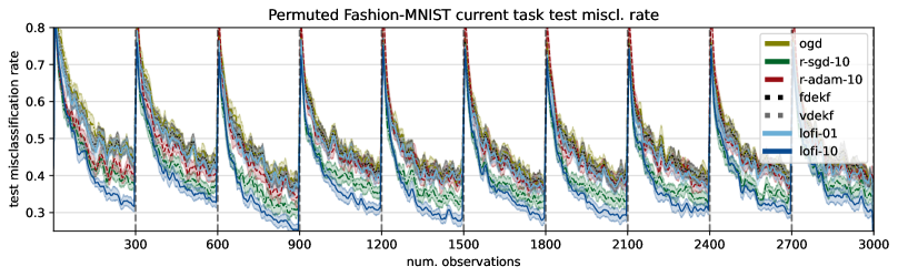
(c)

Figure 1: Test set misclassification rate vs number of observations on (a) the static fashion-MNIST dataset. Figure generated by generate_stationary_clf_plots.ipynb (b) Gradually rotating fashion-MNIST. Figure generated by generate_rotated_clf_plots.ipynb (c) Piecewise stationary permuted fashion-MNIST. The task boundaries are denoted by vertical lines. We show performance on the current task. Figure generated by generate_permuted_clf_plots.ipynb

We start by considering the fashion-MNIST image classification dataset (Xiao et al. (2017)). For replay-SGD, we use a replay buffer of size $10$ and tune the learning rate. In fig. 1(a) we plot the misclassification rate on the test set vs number of training samples using the MLP. (We show the mean and standard error over 100 random trials.) We see that LOFI (with $L=10$) is the most sample efficient learner, then replay SGD (with $B=10$), then replay Adam; the diagonal EKF versions and OGD are the least sample efficient learners.

In the appendix we show the following additional results. In fig. 10(a) we show the results using NLL as the evaluation metric; in this case, the gap between LOFI and the other methods is similarly noticeable. In fig. 10(b) we show the results using NLPD under the generalized probit approximation; the performance gap reduces but LO-FI is still the best method (see appendix B for discussion on analytical approximations to the NLPD). In fig. 11 we show results using a CNN (a LeNet-style architecture with 3 hidden layers and 421,641 parameters); trends are similar to the MLP case. In fig. 12 we show how changing the rank $L$ of LO-FI affects performance within the range 1 to 50. We see that for both NLL and misclassification rate, larger $L$ is better, with gains plateauing at around $L\approx 10$. We also show that a spherical approximation to LO-FI, discussed in appendix F in the appendix, gives worse results.

Piecewise stationary distribution

To evaluate model performance in the non-stationary classification setting, we perform inference under the incremental domain learning scenario using the permuted-fashion-MNIST dataset (Hsu et al., 2018). After every $300$ training examples, the images are permuted randomly and we compare performances across $10$ consecutive tasks.

In fig. 1(c) we plot the performance over the current test set for each task (each test size has size $500$) as a function of the number of training samples. (We show mean and standard error across $20$ random initializations of the dataset). The task boundaries are denoted by vertical dotted lines (this boundary information is not available to the learning agents, and is only used for evaluation). We see that LO-FI rapidly adapts to each new distribution and outperforms all other methods.

In the appendix we show the following additional results. In fig. 13 we show the results using NLL as the evaluation metric; in this case, the gap between LOFI and the other methods is even larger. In fig. 14, we show misclassification for the current task as a function of LO-FI rank; as before, performance increases with rank, and plateaus at $L=10$. In fig. 17, we show results on split fashion MNIST (Hsu et al., 2018), in which each task corresponds to a new pair of classes. However, since this is such an easy task that all methods are effectively indistinguishable.

Slowly changing distribution

The above experiments simulate an unusual form of non-stationarity, corresponding to a sudden change in the task. In this section, we consider a slowly changing distribution, where the task is to classify the images as they slowly rotate. The angle of rotation $\alpha_{t}$ gradually drifts according to an Ornstein-Uhlenbeck process, so $d\alpha_{t}=-\theta(\mu-\alpha_{t})dt+\sigma dW_{t}$, where $W_{t}$ is a white noise process, $\mu=45$, $\sigma=15$, $\theta=10$ and $dt=1/N$, where $N=2000$ is the number of examples. The test-set is modified using the same rotation at each step, perturbed by a Gaussian noise with standard deviation of $5$ degrees. To evaluate performance we use a sliding window of size $200$ around the current time point. The misclassification results are shown in fig. 1(b). LO-FI adapts to the continuously changing environment quickly and outperforms the other methods. In fig. 18 in the appendix we show the NLL and NLPD, which shows a similar trend.

4.2 Regression

In this section, we consider regression tasks using variants of the fashion-MNIST dataset (images from class 2), where we artificially rotate the images, and seek to predict the angle of rotation. As in the classification setting, we use a 2-hidden layer MLP with 500 units per layer.

Stationary distribution

We start by sampling an iid dataset of images, where the angle of rotation at time $t$ is sampled from a uniform ${\cal U}[0,180]$ distribution. In Figure fig. 2(a), we show the RMSE over the test set as a function of the number of trained examples; we see that LOFI outperforms the other methods by a healthy margin. (The NLL and NLPD results in fig. 19 show a similar trend.)

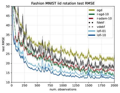
(a)

(b)

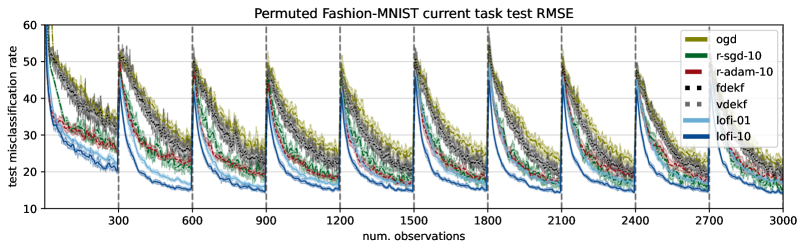
(c)

Figure 2: Test set regression error (measured using RMSE), computed using plugin approximation on various datasets. (a) Static iid distribution of rotated MNIST images. Figure generated by generate_iid_reg_plots.ipynb (b) Slowly changing version of rotated MNIST. Figure generated by generate_rw_reg_plots.ipynb (c) Piecewise stationary permuted roated MNIST. The task boundaries are denoted by vertical lines. We show performance on the current task. Figure generated by generate_permuted_reg_plots.ipynb

Piecewise stationary distribution

We introduce nonstationarity through discrete task changes: we randomly permute the fashion-MNIST dataset after every $300$ training examples, for a total of $10$ tasks. This is similar to the classification setting of section 4.2, except the prediction target is the angle, which is randomly sampled from $(0,180)$ degrees. The goal is to predict the rotation angle of test-set images with the same permutation as the current task. The results are shown in fig. 2(c). We see that LO-FI outperforms all other methods.

Slowly changing distribution

To simulate an arguably more realistic kind of change, we consider the case where the rotation angle slowly changes, generated via an Ornstein-Uhlenbeck process as in section 4.1, except with parameters $\mu=90,\sigma=30$. To evaluate performance we use a sliding window of size $200$, applied to the test set whose rotations are generated by the same rotations as the training set, except perturbed by a Gaussian noise with standard deviation of $5$ degrees. We show the results in fig. 2(b). We see that LO-FI outperforms the baseline methods.

Results on stationary UCI regression benchmark

(a)

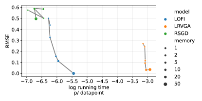
(b)

Figure 3: (a) RMSE vs number of examples on the UCI energy dataset. We show the mean and standard error across 20 partitions. Figure generated by plots-xval.ipynb (b) RMSE vs log running time per data point averaged over multiple UCI regression datasets. The speedup of LOFI compared to LRVGA is about $e^{3}\approx 20$. Figure generated by time-analysis.ipynb

In this section, we evaluate various methods on the UCI tabular regression benchmarks used in several other BNN papers (e.g., (Hernández-Lobato & Adams, 2015; Gal & Ghahramani, 2016; Mishkin et al., 2018)). We use the same splits as in (Gal & Ghahramani, 2016). As in these prior works, we consider an MLP with 1 hidden layer of $H=50$ units using RELU activation, so the number of parameters is $P=(D+2)H+1$, where $D$ is the number of input features. In Table 1 in the appendix, we show the number of features in each dataset, as well as the number of training and testing examples in each of the 20 partitions.

We use these small datasets to compare LO-FI with LRVGA, as well as the other baselines. We show the RMSE vs number of training examples for the Energy dataset in fig. 3(a). In this case, we see that LO-FI (rank 10) outperforms LRVGA (rank 10), and both outperform diagonal EKF and SGD-RB (buffer size 10). However, full covariance EKF is the most sample efficient learner. On other UCI datasets, LRVGA can slightly outperform LO-FI (see section D.1 for details). However, it is about 20 times slower than LOFI. This is visualized in fig. 3(b), which shows RMSE vs compute time, averaged over the 8 UCI datasets listed in table 1. This shows that, controlling for compute costs, LO-FI is a more efficient estimator, and both outperform replay SGD.

4.3 Contextual bandits

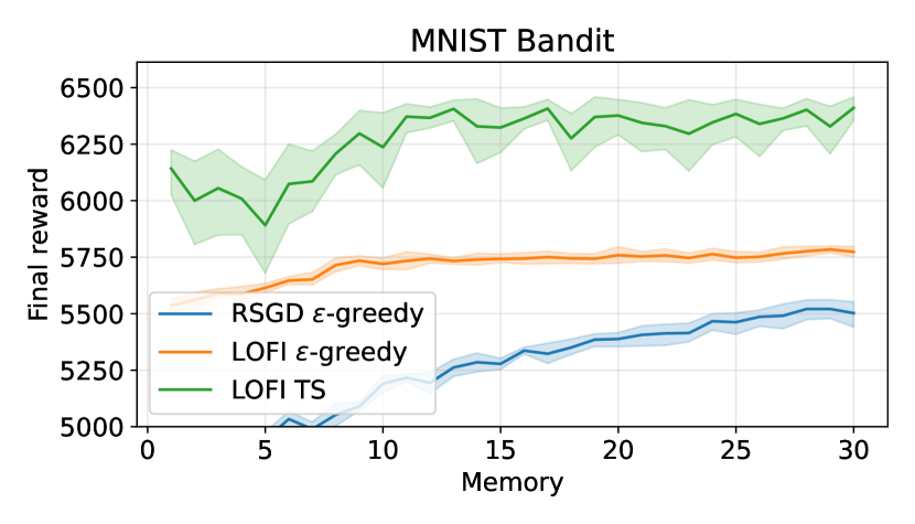
Figure 4: Total reward on MNIST bandit problem after 8000 steps vs memory of the posterior approximation. We show results (averaged over 5 trials) using Thompson sampling or $\epsilon$-greedy with $\epsilon=0.1$. See text for details. Figure generated by bandit-vs-memory.ipynb

In this section, we illustrate the utility of an online Bayesian inference method by applying it to a contextual bandit problem. Following prior work (e.g., (Duran-Martin et al., 2022)), we convert the MNIST classification problem into a bandit problem by defining the action space as a label from 0 to 9, and defining the reward to be 1 if the correct label is predicted, and 0 otherwise. For simplicity, we model this using a nonlinear Gaussian regression model, rather than a nonlinear Bernoulli classification model. To tackle the exploration-exploration tradeoff, we either use Thompson sampling (TS) or the simpler $\epsilon$-greedy baseline. In TS, we sample a parameter from the posterior, $\tilde{{\bm{\theta}}}_{t}\sim p({\bm{\theta}}_{t}|a_{1:t-1},{\bm{x}}_{1:t-1}),r_{1:t-1})$ and then take the greedy action with this value plugged in, $a_{t}=\operatornamewithlimits{argmax}_{a}E[r|{\bm{x}}_{t},\tilde{{\bm{\theta}}}_{t}]$. This method is known to obtain optimal regret (Russo et al., 2018), although the guarantees are weaker when using approximate inference (Phan et al., 2019). Of course, TS requires access to a posterior distribution to sample from. To compare to methods (such as SGD) that just compute a point estimate, we also use $\epsilon$-greedy; in this approach, with probability $\epsilon=0.1$ we try a random action (to encourage exploration), and with probability $1-\epsilon$ we pick the best action, as predicted by plugging in the MAP parameters into the reward model.

In fig. 4, we compare these algorithms on the MNIST bandit problem, where the regression model is a simple MLP with the same architecture as shown in Figure 1b of (Duran-Martin et al., 2022). For the $\epsilon$-greedy exploration policy we use $\epsilon=0.1$, where the MAP parameter estimate is either computed using LO-FI (where the rank is on the $x$-axis) or using SGD with replay buffer (where the buffer size is on the $x$-axis). We also show results of using TS with LO-FI. We see see that TS is much better than $\epsilon$-greedy with LOFI MAP estimate, which in turn is better than $\epsilon$-greedy with SGD MAP estimate. In fig. 22 in the appendix, we plot reward vs time for these methods.

5 Conclusion and future work

We have presented an efficient new method of fitting neural networks online to streaming datasets, using a diagonal plus low-rank Gaussian approximation. In the future, we are interested in developing online methods for estimating the hyper-parameters, perhaps by extending the variational Bayes approach of (Huang et al., 2020; de Vilmarest & Wintenberger, 2021), or the gradient based method of (Greenberg et al., 2021). We would also like to further explore the predictive uncertainty created by our posterior approximation, to see if it can be used for sequential decision making tasks, such as Bayesian optimization or active learning. This may require the use of (online) deep Bayesian ensembles, to capture functional as well as parametric uncertainty.

Appendix A Derivations

A.1 Predict step

We begin with the posterior from the previous time step

$$p({\bm{\theta}}_{t-1}|{\mathcal{D}}_{1:t-1})=\mathcal{N}\left({\bm{\theta}}_{t-1}|\bm{\mu}_{t-1},\left(\bm{\Upsilon}_{t-1}+\mathbf{W}_{t-1}\mathbf{W}_{t-1}^{\mkern-1.5mu\mathsf{T}}\right)^{-1}\right)$$ (13)

and the dynamic assumption

$$p({\bm{\theta}}_{t}|{\bm{\theta}}_{t-1})=\mathcal{N}({\bm{\theta}}_{t}|\gamma_{t}{\bm{\theta}}_{t-1},q_{t}\mathbf{I}_{P})$$ (14)

These imply the prior on the current time step is $p({\bm{\theta}}_{t}|{\mathcal{D}}_{1:t-1})=\mathcal{N}({\bm{\theta}}_{t}|\bm{\mu}_{t|t-1},\bm{\Sigma}_{t|t-1})$ with

$$\bm{\mu}_{t|t-1} =\gamma_{t}\bm{\mu}_{t-1}$$ (15)

$$\bm{\Sigma}_{t|t-1} =\gamma_{t}^{2}\left(\bm{\Upsilon}_{t-1}+\mathbf{W}_{t-1}\mathbf{W}_{t-1}^{\mkern-1.5mu\mathsf{T}}\right)^{-1}+q_{t}\mathbf{I}_{P}$$ (16)

Applying the Woodbury identity to eq. 16 gives this expression for the prior covariance:

$$\bm{\Sigma}_{t|t-1} =\gamma_{t}^{2}\left(\bm{\Upsilon}_{t-1}^{-1}-\bm{\Upsilon}_{t-1}^{-1}\mathbf{W}_{t-1}\left(\mathbf{I}_{L}+\mathbf{W}_{t-1}^{{\mkern-1.5mu\mathsf{T}}}\bm{\Upsilon}_{t-1}^{-1}\mathbf{W}_{t-1}\right)^{-1}\mathbf{W}_{t-1}^{{\mkern-1.5mu\mathsf{T}}}\bm{\Upsilon}_{t-1}^{-1}\right)+q_{t}\mathbf{I}_{P}$$ (17)

$$=\bm{\Upsilon}_{t|t-1}^{-1}-\bm{\Upsilon}_{t-1}^{-1}\mathbf{W}_{t-1}\mathbf{B}_{t|t-1}\mathbf{W}_{t-1}^{{\mkern-1.5mu\mathsf{T}}}\bm{\Upsilon}_{t-1}^{-1}$$ (18)

where

$$\bm{\Upsilon}_{t|t-1} =\left(\gamma_{t}^{2}\bm{\Upsilon}_{t-1}^{-1}+q_{t}\mathbf{I}_{P}\right)^{-1}$$ (19)

$$\mathbf{B}_{t|t-1} =\gamma_{t}^{2}\left(\mathbf{I}_{L}+\mathbf{W}_{t-1}^{{\mkern-1.5mu\mathsf{T}}}\bm{\Upsilon}_{t-1}^{-1}\mathbf{W}_{t-1}\right)^{-1}$$ (20)

Applying Woodbury again yields this expression for the prior precision:

$$\bm{\Sigma}_{t|t-1}^{-1} =\left(\bm{\Upsilon}_{t|t-1}^{-1}-\bm{\Upsilon}_{t-1}^{-1}\mathbf{W}_{t-1}\mathbf{B}_{t|t-1}\mathbf{W}_{t-1}^{{\mkern-1.5mu\mathsf{T}}}\bm{\Upsilon}_{t-1}^{-1}\right)^{-1}$$ (21)

$$=\bm{\Upsilon}_{t|t-1}+\bm{\Upsilon}_{t|t-1}\bm{\Upsilon}_{t-1}^{-1}\mathbf{W}_{t-1}\left(\mathbf{B}_{t|t-1}^{-1}-\mathbf{W}_{t-1}^{{\mkern-1.5mu\mathsf{T}}}\bm{\Upsilon}_{t-1}^{-1}\bm{\Upsilon}_{t|t-1}\bm{\Upsilon}_{t-1}^{-1}\mathbf{W}_{t-1}\right)^{-1}\mathbf{W}_{t-1}^{{\mkern-1.5mu\mathsf{T}}}\bm{\Upsilon}_{t-1}^{-1}\bm{\Upsilon}_{t|t-1}$$ (22)

$$=\bm{\Upsilon}_{t|t-1}+\mathbf{W}_{t|t-1}\mathbf{W}_{t|t-1}^{{\mkern-1.5mu\mathsf{T}}}$$ (23)

where

$$\mathbf{W}_{t|t-1} =\bm{\Upsilon}_{t|t-1}\bm{\Upsilon}_{t-1}^{-1}\mathbf{W}_{t-1}{\rm chol}\left(\left(\mathbf{B}_{t|t-1}^{-1}-\mathbf{W}_{t-1}^{{\mkern-1.5mu\mathsf{T}}}\bm{\Upsilon}_{t-1}^{-1}\bm{\Upsilon}_{t|t-1}\bm{\Upsilon}_{t-1}^{-1}\mathbf{W}_{t-1}\right)^{-1}\right)$$ (24)

$$=\gamma_{t}\bm{\Upsilon}_{t|t-1}\bm{\Upsilon}_{t-1}^{-1}\mathbf{W}_{t-1}\,{\rm chol}\left(\left(\mathbf{I}_{L}+q_{t}\mathbf{W}_{t-1}^{{\mkern-1.5mu\mathsf{T}}}\bm{\Upsilon}_{t|t-1}\bm{\Upsilon}_{t-1}^{-1}\mathbf{W}_{t-1}\right)^{-1}\right)$$ (25)

Calculating $\bm{\Upsilon}_{t|t-1}$ and $\mathbf{W}_{t|t-1}$ respectively take $O(P)$ and $O(PL^{2}+L^{3})$ time. See algorithm 4 for the pseudocode; this is the same as algorithm 2 except we replace $\mathbf{W}_{t}$ with $\mathbf{U}_{t}\bm{\Lambda}_{t}$, as a stepping stone to the spherical version in appendix F.

1def $\text{predict}(\bm{\mu}_{t-1},\bm{\Upsilon}_{t-1},\bm{\Lambda}_{t-1},\mathbf{U}_{t-1},{\bm{x}}_{t},\gamma_{t},q_{t})$:

2 $\mathbf{W}_{t-1}=\mathbf{U}_{t-1}\bm{\Lambda}_{t-1}$ // Recreate the low-rank precision

3 $\bm{\mu}_{t|t-1}=\gamma\bm{\mu}_{t-1}$ // Predict the mean of the next state

4 $\bm{\Upsilon}_{t|t-1}=\left(\gamma_{t}^{2}\bm{\Upsilon}_{t-1}^{-1}+q_{t}\mathbf{I}_{P}\right)^{-1}$ // Predict the diagonal precision

5 $\mathbf{C}_{t}=\left(\mathbf{I}_{L}+q_{t}\mathbf{W}_{t-1}^{{\mkern-1.5mu\mathsf{T}}}\bm{\Upsilon}_{t|t-1}\bm{\Upsilon}_{t-1}^{-1}\mathbf{W}_{t-1}\right)^{-1}$

6 $\mathbf{W}_{t|t-1}=\gamma_{t}\bm{\Upsilon}_{t|t-1}\bm{\Upsilon}_{t-1}^{-1}\mathbf{W}_{t-1}{\rm chol}(\mathbf{C}_{t})$ // Predict the low-rank precision

7 $\mathbf{U}_{t|t-1}=\mathbf{W}_{t|t-1}$ // For compatibility with spherical LO-FI

8 $\bm{\Lambda}_{t|t-1}=\bm{1}$ // Arbitrary scaling

9 $\hat{{\bm{y}}}_{t}=h\left({\bm{x}}_{t},\bm{\mu}_{t|t-1}\right)$ // Predict the mean of the output

Return $(\bm{\mu}_{t|t-1},\bm{\Upsilon}_{t|t-1},\bm{\Lambda}_{t|t-1},\mathbf{U}_{t|t-1},\hat{{\bm{y}}}_{t})$

Algorithm 4 LO-FI predict step.

A.2 Update step

After creating a linear-Gaussian approximation to the likelihood (as explained in the main text), standard results (see e.g., Sarkka & Svensson, 2023) imply the exact posterior can be written as $p({\bm{\theta}}_{t}|{\mathcal{D}}_{1:t})=\mathcal{N}({\bm{\theta}}_{t}|\bm{\mu}_{t},\bm{\Sigma}_{t}^{*})$, where

$$\bm{\Sigma}_{t}^{*-1} =\bm{\Sigma}_{t|t-1}^{-1}+\mathbf{H}_{t}^{\mkern-1.5mu\mathsf{T}}\mathbf{R}_{t}^{-1}\mathbf{H}_{t}$$ (26)

$$\mathbf{K}_{t} =\bm{\Sigma}_{t}^{*}\mathbf{H}_{t}^{\mkern-1.5mu\mathsf{T}}\mathbf{R}_{t}^{-1}$$ (27)

$${\bm{e}}_{t} ={\bm{y}}_{t}-\hat{{\bm{y}}}_{t}$$ (28)

$$\bm{\mu}_{t} =\bm{\mu}_{t|t-1}+\mathbf{K}_{t}{\bm{e}}_{t}$$ (29)

where $\mathbf{K}_{t}$ is known as the Kalman gain matrix, and ${\bm{e}}_{t}$ is the innovation vector (i.e., error in the prediction).

We now derive a low-rank version of the above update equations. Because $\mathbf{R}_{t}$ is positive-definite, we can write $\mathbf{R}_{t}^{-1}=\mathbf{A}_{t}^{\mkern-1.5mu\mathsf{T}}\mathbf{A}_{t}$. We then define the matrix

$$\tilde{\mathbf{W}}_{t}=\left[\begin{array}[]{cc}\mathbf{W}_{t|t-1}&\mathbf{H}_{t}^{{\mkern-1.5mu\mathsf{T}}}\mathbf{A}_{t}^{{\mkern-1.5mu\mathsf{T}}}\end{array}\right]$$ (31)

This has size $P\times\tilde{L}$, where $\tilde{L}=L+C$. Note that if the output is scalar, with variance $R=\sigma^{2}$, we have $\mathbf{H}_{t}=\nabla_{{\bm{\theta}}_{t}}h({\bm{x}}_{t},{\bm{\theta}}_{t})$. For a linear model, $h({\bm{x}}_{t},{\bm{\theta}}_{t})={\bm{\theta}}_{t}^{\mkern-1.5mu\mathsf{T}}{\bm{x}}_{t}$, the gradient equals the data vector ${\bm{x}}_{t}$. In this case, we have

$$\tilde{\mathbf{W}}_{t}=\left[\begin{array}[]{cc}\mathbf{W}_{t|t-1}&\frac{1}{\sigma}{\bm{x}}_{t}\end{array}\right]$$ (33)

Thus $\tilde{\mathbf{W}}_{t}$ acts like a generalized memory buffer that stores data using a gradient embedding.

From eq. 26, the exact Bayesian inference step for the precision is

$$\bm{\Sigma}_{t}^{*-1} =\bm{\Sigma}_{t|t-1}^{-1}+\mathbf{H}_{t}^{{\mkern-1.5mu\mathsf{T}}}\mathbf{A}_{t}^{{\mkern-1.5mu\mathsf{T}}}\mathbf{A}_{t}\mathbf{H}_{t}$$ (34)

$$=\bm{\Upsilon}_{t|t-1}+\mathbf{W}_{t|t-1}\mathbf{W}_{t|t-1}^{\mkern-1.5mu\mathsf{T}}+\mathbf{H}_{t}^{{\mkern-1.5mu\mathsf{T}}}\mathbf{A}_{t}^{{\mkern-1.5mu\mathsf{T}}}\mathbf{A}_{t}\mathbf{H}_{t}$$ (35)

$$=\bm{\Upsilon}_{t|t-1}+\tilde{\mathbf{W}}_{t}\tilde{\mathbf{W}}_{t}^{{\mkern-1.5mu\mathsf{T}}}$$ (36)

From eqs. 27, 28 and 29, the exact mean update is given by

$$\bm{\mu}_{t}=\bm{\mu}_{t|t-1}+\bm{\Sigma}_{t}^{*}\mathbf{H}_{t}^{{\mkern-1.5mu\mathsf{T}}}\mathbf{R}_{t}^{-1}{\bm{e}}_{t}$$ (37)

Applying the Woodbury identity to eq. 36 and substituting into eq. 37, we obtain an expression that can be computed in $O(P\tilde{L}^{2})$ time:

$$\bm{\mu}_{t}=\bm{\mu}_{t|t-1}+\left(\bm{\Upsilon}_{t|t-1}^{-1}-\bm{\Upsilon}_{t|t-1}^{-1}\tilde{\mathbf{W}}_{t}\left(\mathbf{I}_{\tilde{L}}+\tilde{\mathbf{W}}_{t}^{{\mkern-1.5mu\mathsf{T}}}\bm{\Upsilon}_{t|t-1}^{-1}\tilde{\mathbf{W}}_{t}\right)^{-1}\tilde{\mathbf{W}}_{t}^{{\mkern-1.5mu\mathsf{T}}}\bm{\Upsilon}_{t|t-1}^{-1}\right)\mathbf{H}_{t}^{{\mkern-1.5mu\mathsf{T}}}\mathbf{R}_{t}^{-1}{\bm{e}}_{t}$$ (38)

Equations 36 and 38 give the exact posterior, given the DLR($L$) prior. However, to propagate this posterior to the next step, we need to project $\bm{\Sigma}_{t}^{*-1}$ from $\text{DLR}(\tilde{L})$ back to $\text{DLR}(L)$. To do this, we first perform an SVD of $\tilde{\mathbf{W}}_{t}$ to get the new basis:

$$(\tilde{\bm{\Lambda}}_{t},\tilde{\mathbf{U}}_{t}) ={\rm SVD}(\tilde{\mathbf{W}}_{t})$$ (39)

$$\mathbf{W}_{t} =\left(\tilde{\mathbf{U}}_{t}\tilde{\bm{\Lambda}}_{t}\right)[:,1{:}L]$$ (40)

Here, $\tilde{\bm{\Lambda}}_{t}$ and $\tilde{\mathbf{U}}_{t}$ are respectively the singular values and left singular vectors of $\tilde{\mathbf{W}}_{t}$, assumed to be ordered in decreasing value of $\tilde{\bm{\Lambda}}_{t}$ (so $\tilde{\bm{\Lambda}}_{t}$ is diagonal of size $\tilde{L}\times\tilde{L}$, and $\tilde{\mathbf{U}}_{t}$ is of size $P\times\tilde{L}$). Finally, we update the diagonal term as follows:

$$\bm{\Upsilon}_{t} =\bm{\Upsilon}_{t|t-1}+\mathrm{diag}\left(\mathbf{W}_{t}^{\times}\mathbf{W}_{t}^{\times{\mkern-1.5mu\mathsf{T}}}\right)$$ (41)

$$\mathbf{W}_{t}^{\times} =\left(\tilde{\mathbf{U}}_{t}\tilde{\bm{\Lambda}}_{t}\right)[:,(L+1){:}\tilde{L}]$$ (42)

Adding the diagonal contribution from the remaining $C$ singular vectors to $\bm{\Upsilon}_{t}$ ensures the diagonal portion of the DLR approximation is exact, i.e.,

$$\mathrm{diag}(\bm{\Sigma}_{t}^{-1})=\mathrm{diag}(\bm{\Sigma}_{t}^{*-1}).$$ (43)

See algorithm 5 for the pseudocode. This is the same as algorithm 3 except we replace $\mathbf{W}_{t}$ with $\mathbf{U}_{t}\bm{\Lambda}_{t}$. This procedure takes $O(P\tilde{L}^{2})$ time for the SVD, and $O(PC)$ for calculating $\mathrm{diag}\left(\mathbf{W}_{t}^{\times}\mathbf{W}_{t}^{\times{\mkern-1.5mu\mathsf{T}}}\right)$.

1def $\text{update}(\bm{\mu}_{t|t-1},\bm{\Upsilon}_{t|t-1},\bm{\Lambda}_{t|t-1},\mathbf{U}_{t|t-1},{\bm{x}}_{t},{\bm{y}}_{t},\hat{{\bm{y}}}_{t},h,L)$:

2 $\mathbf{R}_{t}=h_{V}({\bm{x}}_{t},\bm{\mu}_{t|t-1})$ // Covariance of predicted output

3 $\mathbf{L}_{t}=\text{chol}(\mathbf{R}_{t})$

4 $\mathbf{A}_{t}=\mathbf{L}_{t}^{-1}$

5 $\mathbf{H}_{t}=\text{jac}(h({\bm{x}}_{t},\cdot))(\bm{\mu}_{t|t-1})$ // Jacobian of observation model

6 $\mathbf{W}_{t|t-1}=\mathbf{U}_{t|t-1}\bm{\Lambda}_{t|t-1}$ // Predicted low-rank precision

7 $\tilde{\mathbf{W}}_{t}=\left[\begin{array}[]{cc}\mathbf{W}_{t|t-1}&\mathbf{H}_{t}^{{\mkern-1.5mu\mathsf{T}}}\mathbf{A}_{t}^{{\mkern-1.5mu\mathsf{T}}}\end{array}\right]$ // Expand low-rank with new observation

8 $\mathbf{G}_{t}=\left(\mathbf{I}_{\tilde{L}}+\tilde{\mathbf{W}}_{t}^{{\mkern-1.5mu\mathsf{T}}}\bm{\Upsilon}_{t|t-1}^{-1}\tilde{\mathbf{W}}_{t}\right)^{-1}$

9 $\mathbf{C}_{t}=\mathbf{H}_{t}^{{\mkern-1.5mu\mathsf{T}}}\mathbf{A}_{t}^{\mkern-1.5mu\mathsf{T}}\mathbf{A}_{t}$

10 $\mathbf{K}_{t}=\bm{\Upsilon}_{t|t-1}^{-1}\mathbf{C}_{t}-\bm{\Upsilon}_{t|t-1}^{-1}\tilde{\mathbf{W}}_{t}\mathbf{G}_{t}\tilde{\mathbf{W}}_{t}^{{\mkern-1.5mu\mathsf{T}}}\bm{\Upsilon}_{t|t-1}^{-1}\mathbf{C}_{t}$ // Kalman gain matrix

11 $\bm{\mu}_{t}=\bm{\mu}_{t|t-1}+\mathbf{K}_{t}({\bm{y}}_{t}-\hat{{\bm{y}}}_{t})$ // Mean update

12 $(\tilde{\bm{\Lambda}}_{t},\tilde{\mathbf{U}}_{t})={\rm SVD}(\tilde{\mathbf{W}}_{t})$ // Take SVD of the expanded low-rank

13 $(\bm{\Lambda}_{t},\mathbf{U}_{t})=\left(\tilde{\bm{\Lambda}}_{t},\tilde{\mathbf{U}}_{t}\right)[:,1{:}L]$ // Keep top $L$ most important terms

14 $(\bm{\Lambda}_{t}^{\times},\mathbf{U}_{t}^{\times})=\left(\tilde{\bm{\Lambda}}_{t},\tilde{\mathbf{U}}_{t}\right)[:,(L+1){:}\tilde{L}]$ // Extra least important terms

15 $\mathbf{W}_{t}^{\times}=\mathbf{U}_{t}^{\times}\bm{\Lambda}_{t}^{\times}$ // The low-rank part that is dropped

16 $\bm{\Upsilon}_{t}=\bm{\Upsilon}_{t|t-1}+\mathrm{diag}\left(\mathbf{W}_{t}^{\times}(\mathbf{W}_{t}^{\times})^{{\mkern-1.5mu\mathsf{T}}}\right)$ // Update diagonal to capture variance due to dropped terms

Return $(\bm{\mu}_{t},\bm{\Upsilon}_{t},\bm{\Lambda}_{t},\mathbf{U}_{t})$

Algorithm 5 LO-FI update step.

A.3 Alternative diagonal update

Instead of updating $\bm{\Upsilon}_{t}$ to achieve $\mathrm{diag}(\bm{\Sigma}_{t}^{-1})=\mathrm{diag}(\bm{\Sigma}_{t}^{*-1})$, we can minimize the KL divergence. If we define

$$\bm{\Upsilon}_{t}=\operatornamewithlimits{argmin}_{\bm{\Upsilon}}D_{\mathbb{KL}}\left({\mathcal{N}\left(\bm{\mu}_{t},\left(\bm{\Upsilon}+\mathbf{W}_{t}\mathbf{W}_{t}^{\mkern-1.5mu\mathsf{T}}\right)^{-1}\right)}\mathrel{\|}{\mathcal{N}(\bm{\mu}_{t},\bm{\Sigma}_{t}^{*})}\right)$$ (44)

then we get the condition

$$\mathrm{diag}(\bm{\Sigma}_{t}-\bm{\Sigma}_{t}\bm{\Sigma}_{t}^{*-1}\bm{\Sigma}_{t})=0$$ (45)

If instead we use forward KL,

$$\bm{\Upsilon}_{t}=\operatornamewithlimits{argmin}_{\bm{\Upsilon}}D_{\mathbb{KL}}\left({\mathcal{N}(\bm{\mu}_{t},\bm{\Sigma}_{t}^{*})}\mathrel{\|}{\mathcal{N}\left(\bm{\mu}_{t},\left(\bm{\Upsilon}+\mathbf{W}_{t}\mathbf{W}_{t}^{\mkern-1.5mu\mathsf{T}}\right)^{-1}\right)}\right)$$ (46)

then we get the condition

$$\mathrm{diag}(\bm{\Sigma}_{t})=\mathrm{diag}(\bm{\Sigma}_{t}^{*})$$ (47)

We leave exploration of possible efficient implementations of these updates to future work.

A.4 Zero-rank LO-FI

When $L=0$, LO-FI approximates the covariance simply as

$$\bm{\Sigma}_{t}=\bm{\Upsilon}_{t}^{-1}$$ (48)

Consequently, the predict step comprises only eqs. 15 and 19, repeated here:

$$\bm{\mu}_{t|t-1} =\gamma_{t}{\bm{\mu}}_{t-1}$$ (49)

$$\bm{\Upsilon}_{t|t-1} =\left(\gamma_{t}^{2}{\bm{\Upsilon}}_{t-1}^{-1}+q_{t}\mathbf{I}_{P}\right)^{-1}$$ (50)

In the update step, $\mathbf{W}_{t|t-1}$ is empty, so $\mathbf{W}_{t}^{\times}=\tilde{\mathbf{W}}_{t}=\mathbf{H}_{t}^{\mkern-1.5mu\mathsf{T}}\mathbf{A}_{t}^{\mkern-1.5mu\mathsf{T}}$. Therefore eqs. 38 and 41 become

$$\bm{\mu}_{t} =\bm{\mu}_{t|t-1}+\bm{\Upsilon}_{t|t-1}^{-1}\mathbf{H}_{t}^{\mkern-1.5mu\mathsf{T}}\left(\mathbf{H}_{t}\bm{\Upsilon}_{t|t-1}^{-1}\mathbf{H}_{t}^{\mkern-1.5mu\mathsf{T}}+\mathbf{R}_{t}\right)^{-1}{\bm{e}}_{t}$$ (51)

$$\bm{\Upsilon}_{t} =\bm{\Upsilon}_{t|t-1}+\mathrm{diag}(\mathbf{H}_{t}^{\mkern-1.5mu\mathsf{T}}\mathbf{R}_{t}^{-1}\mathbf{H}_{t})$$ (52)

Finally, in the predictive distribution for the observation, the variance in eq. 63 simplifies:

$$\hat{{\bm{y}}}_{t} =h({\bm{x}}_{t},\bm{\mu}_{t|t-1})$$ (53)

$$\mathbf{V}_{t} =\mathbf{H}_{t}\bm{\Upsilon}_{t|t-1}^{-1}\mathbf{H}_{t}^{{\mkern-1.5mu\mathsf{T}}}+\mathbf{R}_{t}$$ (54)

These equations match those of the VD-EKF (Chang et al., 2022), confirming that LO-FI reduces to VD-EKF when $L=0$.

Appendix B Posterior predictive distribution for the observations

In this section, we discuss how to use the posterior over parameters to approximate the posterior predictive distribution for the observations:

$$p({\bm{y}}_{t}|{\bm{x}}_{t},{\mathcal{D}}_{1:t-1}) =\int p({\bm{y}}_{t}|{\bm{x}}_{t},{\bm{\theta}}_{t})p({\bm{\theta}}_{t}|{\mathcal{D}}_{1:t-1})d{\bm{\theta}}_{t}$$ (55)

A simple approach is to use a plugin approximation, which arises when we assume the posterior is a point estimate:

$$p({\bm{y}}_{t}|{\bm{x}}_{t},{\mathcal{D}}_{1:t-1}) \approx\int p({\bm{y}}_{t}|{\bm{x}}_{t},{\bm{\theta}}_{t})\delta({\bm{\theta}}_{t}-\hat{{\bm{\theta}}}_{t})d{\bm{\theta}}_{t}$$ (56)

$$=\begin{cases}\mathcal{N}({\bm{y}}_{t}|h({\bm{x}}_{t},\hat{{\bm{\theta}}}_{t}),\mathbf{R}_{t})&\mbox{regression}\\ \mathrm{Cat}({\bm{y}}_{t}|\mathrm{softmax}(h({\bm{x}}_{t},\hat{{\bm{\theta}}}_{t}))&\mbox{classification}\end{cases}$$ (57)

We can capture more uncertainty by sampling parameters from the (Gaussian) posterior, ${\bm{\theta}}_{t}^{s}\sim\mathcal{N}(\bm{\mu}_{t|t-1},\bm{\Sigma}_{t|t-1})$, which results in the following Monte Carlo approximation:

$$p({\bm{y}}_{t}|{\bm{x}}_{t},{\mathcal{D}}_{1:t-1}) \approx\begin{cases}\frac{1}{S}\sum_{s=1}^{S}\mathcal{N}({\bm{y}}_{t}|h({\bm{x}}_{t},{\bm{\theta}}_{t}^{s}),\mathbf{R}_{t})&\mbox{regression}\\ \frac{1}{S}\sum_{s=1}^{S}\mathrm{Cat}({\bm{y}}_{t}|\mathrm{softmax}(h({\bm{x}}_{t},{\bm{\theta}}_{t}^{s}))&\mbox{classification}\end{cases}$$ (58)

If we have a DLR approximation to the precision matrix, we can use the importance sampling method of Section 6.2 of (Lambert et al., 2021a) to draw samples in $O(PS)$ time, without needing to create or invert the full precision matrix.

However, as argued in (Immer et al., 2021), it can sometimes be better to approximate the predictive distribution by first linearizing the observation model, and then passing the samples through the linearized model, to avoid evaluating the nonlinear function with parameter values that are far from the posterior mode. Once we have linearized the model, we can further replace the Monte Carlo approximation with a deterministic integral, as we explain below.

B.1 Deterministic approximation for regression

If we linearize the observation model, and assume a Gaussian output, we can compute the posterior predictive distribution analytically, as follows:

$$p({\bm{y}}_{t}|{\bm{x}}_{t},{\mathcal{D}}_{1:t-1}) =\int p_{\text{lin}}({\bm{y}}_{t}|{\bm{x}}_{t},{\bm{\theta}}_{t})p({\bm{\theta}}_{t}|{\mathcal{D}}_{1:t-1})d{\bm{\theta}}_{t}$$ (59)

$$=\int\mathcal{N}({\bm{y}}_{t}|\hat{h}_{t}({\bm{\theta}}_{t}),\mathbf{R}_{t})\mathcal{N}({\bm{\theta}}_{t}|\bm{\mu}_{t|t-1},\bm{\Sigma}_{t|t-1})d{\bm{\theta}}_{t}$$ (60)

Hence

$$\hat{{\bm{y}}}_{t} =\mathbb{E}\left[{{\bm{y}}_{t}|{\bm{x}}_{t},{\mathcal{D}}_{1:t-1}}\right]=h({\bm{x}}_{t},\bm{\mu}_{t|t-1})$$ (61)

$$\mathbf{V}_{t} =\mathrm{Cov}\left[{{\bm{y}}_{t}|{\bm{x}}_{t},{\mathcal{D}}_{1:t-1}}\right]=\mathbf{H}_{t}\bm{\Sigma}_{t|t-1}\mathbf{H}_{t}^{{\mkern-1.5mu\mathsf{T}}}+\mathbf{R}_{t}$$ (62)

We can rewrite $\mathbf{V}_{t}$ using Woodbury in a form that can be computed in $O(PL^{2})$ time:

$$\mathbf{V}_{t}=\mathbf{H}_{t}\left(\bm{\Upsilon}_{t|t-1}^{-1}-\bm{\Upsilon}_{t|t-1}^{-1}\mathbf{W}_{t|t-1}\left(\mathbf{I}_{L}+\mathbf{W}_{t|t-1}^{\mkern-1.5mu\mathsf{T}}\bm{\Upsilon}_{t|t-1}^{-1}\mathbf{W}_{t|t-1}\right)^{-1}\mathbf{W}_{t|t-1}^{\mkern-1.5mu\mathsf{T}}\bm{\Upsilon}_{t|t-1}^{-1}\right)\mathbf{H}_{t}^{{\mkern-1.5mu\mathsf{T}}}+\mathbf{R}_{t}$$ (63)

B.2 Deterministic approximation for classification

In this section, we consider a classification model: $h({\bm{x}},{\bm{\theta}})=\mathrm{softmax}(f({\bm{x}},{\bm{\theta}}))$, where $f$ is a neural network that outputs a vector of $C$ logits. Following (Immer et al., 2021), suppose we linearize $f$:

$$\hat{f}_{t}({\bm{\theta}})=f({\bm{x}}_{t},\bm{\mu}_{t|t-1})+\mathbf{F}_{t}({\bm{\theta}}-\bm{\mu}_{t|t-1})$$ (64)

where $\mathbf{F}_{t}$ is the Jacobian of $f({\bm{x}}_{t},\cdot)$ at $\bm{\mu}_{t|t-1}$. (This is the analog of $\hat{h}_{t}$ and $\mathbf{H}_{t}$, except we omit the final softmax layer.) Let ${\bm{z}}_{t}=\hat{f}_{t}({\bm{\theta}})$ be the predicted logits. We can now deterministically approximate the predicted probabilities by using the generalized probit approximation (Gibbs, 1997; Daunizeau, 2017):

$${\bm{p}}_{t} =\int\mathrm{softmax}({\bm{z}}_{t})\mathcal{N}({\bm{z}}_{t}|\hat{{\bm{z}}}_{t},\mathbf{F}_{t}\bm{\Sigma}_{t|t-1}\mathbf{F}_{t}^{\mkern-1.5mu\mathsf{T}})d{\bm{z}}_{t}$$ (65)

$$\approx\mathrm{softmax}\left(\left\{\frac{\hat{z}_{t,c}}{\sqrt{1+\frac{\pi}{8}v_{c}}}\right\}\right)$$ (66)

where $v_{c}=[\mathbf{F}_{t}\bm{\Sigma}_{t|t-1}\mathbf{F}_{t}^{\mkern-1.5mu\mathsf{T}}]_{cc}$ is the marginal variance for class $c$. This makes the probabilities “less extreme” (closer to uniform) when the parameters are uncertain. Alternatively, we can use the “Laplace bridge” method of (Hobbhahn et al., 2022), which has been shown to be more accurate than the generalized probit approximation.

Appendix C Tuning the hyper-parameters

In this section, we discuss how to estimate the SSM hyper-parameters, namely the system noise $q$, the system dynamics $\gamma$, and (for regression) the observation noise $R$. We also need to specify the initial belief state $\bm{\mu}_{0}$ (which we sample from a zero-mean Gaussian prior) and $\bm{\Sigma}_{0}=(1/\eta_{0})\mathbf{I}$.

C.1 Bayesian optimization

We optimize the hyper-parameters using black-box Bayesian optimization, using performance on a validation set as the metric for static datasets, and the (averaged) one-step-ahead error as the metric for non-stationary datasets.

C.2 Online adaptation of the hyper-parameters

Offline hyper-parameter tuning using a validation set cannot be applied to non-stationary problems. To tackle this, we can estimate the SSM parameters online; this approach is called adaptive Kalman filtering. As a simple example, we implemented a recursive estimate for $\mathbf{R}_{t}$, based on a running average of the empirical prediction errors, as proposed in Ljung & Soderstrom (1983) and Iiguni et al. (1992):

$$\hat{\mathbf{R}}_{t} =(1-\varepsilon_{t})\hat{\mathbf{R}}_{t-1}+\varepsilon_{t}({\bm{y}}_{t}-\hat{{\bm{y}}}_{t})({\bm{y}}_{t}-\hat{{\bm{y}}}_{t})^{\mkern-1.5mu\mathsf{T}}$$ (67)

where $\varepsilon_{t}>0$ is a learning rate (e.g., $\varepsilon_{t}=\max(\varepsilon_{\min},1/t)$), and $\hat{{\bm{y}}}_{t}=h({\bm{x}}_{t},\bm{\mu}_{t|t-1})$. If $\mathbf{R}_{t}=r_{t}\mathbf{I}$, this becomes

$$\hat{r}_{t} =(1-\varepsilon_{t})\hat{r}_{t-1}+\varepsilon_{t}({\bm{y}}_{t}-\hat{{\bm{y}}}_{t})^{\mkern-1.5mu\mathsf{T}}({\bm{y}}_{t}-\hat{{\bm{y}}}_{t})$$ (68)

To estimate the other hyper-parameters, such as $Q$, in an online way, we may be able to extend the variational Bayes approach of (Huang et al., 2020; de Vilmarest & Wintenberger, 2021), or the gradient based method of (Greenberg et al., 2021). However we leave this to future work.

Appendix D Additional experimental results

D.1 UCI regression

	Num. features	Num. train	Num. test	Num. obs.	Num. parameters
Boston	13	455	51	506	751
Concrete	8	927	103	1030	501
Energy	8	691	77	768	501
Kin8nm	8	7373	819	8192	501
Naval	16	10741	1193	11934	901
Power	4	8611	957	9568	301
Wine	11	1439	160	1599	651
Yacht	6	277	31	308	401

Table 1: UCI regression dataset summary, and the corresponding number of parameters in a single-layered MLP with 50 hidden units.

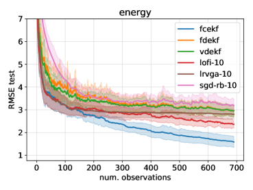
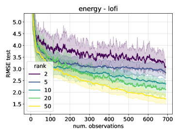
Figure 5: Error vs number of observations on the energy dataset. We show the mean and standard error across 20 partitions. (a) Curves correspind to the following methods: for FCEKF, FDEKF (similar to VDEKF), LO-FI-$10$, LRVGA-$10$, SGD-RB-$10$. (b) Curves correspond to LO-FI with different ranks. Figure generated by plots-xval.ipynb.

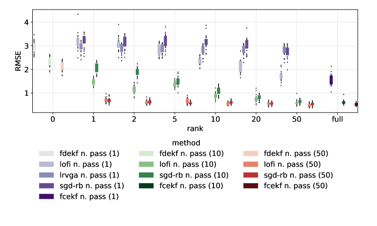
Figure 6: RMSE boxplot for the energy dataset. We compare the performance of different estimators as a function of rank and number of passes over the dataset. (Note that VDEKF is very similar to FDEKF so is not shown.) Figure generated by plots-xval-passes.ipynb

In this section, we evaluate various methods on the UCI tabular regression benchmarks used in several other BNN papers (e.g., (Hernández-Lobato & Adams, 2015; Gal & Ghahramani, 2016; Mishkin et al., 2018)). We use the same splits as in (Gal & Ghahramani, 2016). As in these prior works, we consider an MLP with 1 hidden layer of $H=50$ units using RELU activation, so the number of parameters is $P=(D+2)H+1$, where $D$ is the number of input features. In Table 1, we show the number of features in each dataset, as well as the number of training and testing examples in each of the 20 partitions.

In Figure 5(a) we show the test error vs number of training observations for different estimators on the energy dataset. We see that LO-FI (rank 10) outperforms LRVGA (rank 10), and both outperform diagonal EKF and SGD-RB (buffer size 10). However, full covariance EKF is the most sample efficient learner. In Figure 5(b), we show that increasing the rank of the LO-FI approximation improves performance; by $L=50$ it has essentially matched the full rank case, which uses $P=501$ parameters.

Another way to improve performance is to perform multiple passes over the data, by concatenating the data sequence into a single long stream (shuffling the order at the end of each epoch). The benefits of this approach are shown in fig. 6. The different colors correspond to 1, 10 and 50 passes over the data. (Note that we only performed one pass for LRVGA, since it is significantly slower than all other methods, as shown in fig. 7.) We see that multiple passes consistently improves performance. However this trick can only be used in the offline setting for static distributions. In fig. 6, we also see that the error vs rank decreases faster for LO-FI than for LRVGA and SGD-RB, meaning that it makes better use of its increased posterior accuracy to increase the sample efficiency of the learner.

Results for all the UCI regression datasets for different methods are shown in table 2. As in the energy dataset, we find that increasing the rank helps all low-rank (and memory-based) methods, and increasing the number of passes also helps. In general FECKF is the best, with LO-FI usually in second place. Interestingly we find that spherical LO-FI has comparable performance to diagonal LO-FI, but is faster (see table 6 and fig. 7 for a running time comparison). However, we caution against reading too many conclusions from these results, since the datasets are small, and the error bars overlap a lot between methods.

		dataset	Boston	Concrete	Energy	Kin8nm	Naval	Power	Wine	Yacht
# passes	Rank	Method
1	0	fdekf	$5.23\pm 2.19$	$8.60\pm 0.63$	$2.96\pm 0.25$	$0.12\pm 0.01$	$0.01\pm 0.00$	$4.24\pm 0.16$	$0.82\pm 0.05$	$5.13\pm 1.30$
		vdekf	$9.03\pm 1.18$	$16.35\pm 0.82$	$9.44\pm 0.47$	$0.14\pm 0.01$	$0.01\pm 0.00$	$4.25\pm 0.16$	$0.66\pm 0.05$	$5.60\pm 1.29$
	10	lofi-s	$5.12\pm 1.49$	$7.27\pm 0.89$	$2.36\pm 0.16$	$0.12\pm 0.00$	$0.00\pm 0.00$	$4.20\pm 0.15$	$0.65\pm 0.03$	$4.66\pm 0.83$
		lofi-d	$4.77\pm 1.20$	$7.33\pm 0.89$	$2.53\pm 0.26$	$0.14\pm 0.01$	$0.00\pm 0.00$	$4.37\pm 0.15$	$0.72\pm 0.06$	$4.66\pm 0.83$
		lrvga	$3.62\pm 1.02$	$7.28\pm 0.73$	$2.80\pm 0.22$	$0.12\pm 0.00$	$0.00\pm 0.00$	$4.22\pm 0.15$	$0.65\pm 0.04$	$3.39\pm 0.79$
		sgd-rb	$4.41\pm 1.23$	$8.46\pm 0.77$	$3.18\pm 0.30$	$0.13\pm 0.01$	$0.00\pm 0.00$	$4.81\pm 0.57$	$0.70\pm 0.06$	$7.92\pm 1.27$
	full	fcekf	$4.04\pm 1.07$	$6.45\pm 0.53$	$1.58\pm 0.25$	$0.10\pm 0.00$	$0.00\pm 0.00$	$4.13\pm 0.16$	$0.66\pm 0.04$	$3.14\pm 1.09$
10	0	fdekf	$3.20\pm 0.92$	$6.68\pm 0.51$	$2.32\pm 0.22$	$0.10\pm 0.00$	$0.01\pm 0.00$	$4.18\pm 0.15$	$0.82\pm 0.05$	$1.18\pm 0.36$
		vdekf	$9.03\pm 1.18$	$16.35\pm 0.82$	$10.10\pm 0.47$	$0.11\pm 0.00$	$0.01\pm 0.00$	$4.20\pm 0.16$	$0.64\pm 0.04$	$2.32\pm 0.54$
	10	lofi-s	$5.38\pm 1.36$	$5.63\pm 0.64$	$0.88\pm 0.14$	$0.10\pm 0.00$	$0.00\pm 0.00$	$4.14\pm 0.16$	$0.64\pm 0.04$	$1.51\pm 0.37$
		lofi-d	$5.08\pm 1.29$	$5.86\pm 0.50$	$1.36\pm 0.19$	$0.09\pm 0.00$	$0.00\pm 0.00$	$4.13\pm 0.16$	$0.64\pm 0.04$	$2.26\pm 0.52$
		sgd-rb	$3.63\pm 0.84$	$6.29\pm 0.68$	$1.08\pm 0.18$	$0.10\pm 0.01$	$0.00\pm 0.00$	$4.73\pm 0.38$	$0.71\pm 0.05$	$2.26\pm 0.56$
	full	fcekf	$3.13\pm 0.89$	$5.31\pm 0.48$	$0.62\pm 0.09$	$0.09\pm 0.00$	$0.00\pm 0.00$	$4.05\pm 0.17$	$0.64\pm 0.05$	$1.19\pm 0.27$
50	0	fdekf	$2.95\pm 0.71$	$6.37\pm 0.52$	$2.11\pm 0.21$	$0.09\pm 0.00$	$0.01\pm 0.00$	$4.14\pm 0.16$	$0.82\pm 0.05$	$0.80\pm 0.26$
		vdekf	$9.03\pm 1.18$	$16.35\pm 0.82$	$10.10\pm 0.47$	$0.10\pm 0.00$	$0.01\pm 0.00$	$4.17\pm 0.16$	$0.63\pm 0.04$	$1.62\pm 0.37$
	10	lofi-s	$5.29\pm 1.12$	$5.41\pm 0.64$	$0.56\pm 0.07$	$0.09\pm 0.00$	$0.00\pm 0.00$	$4.06\pm 0.17$	$0.66\pm 0.05$	$0.92\pm 0.27$
		lofi-d	$4.99\pm 1.10$	$5.53\pm 0.50$	$0.86\pm 0.14$	$0.09\pm 0.00$	$0.00\pm 0.00$	$4.10\pm 0.16$	$0.63\pm 0.04$	$1.36\pm 0.33$
		sgd-rb	$3.52\pm 0.68$	$5.78\pm 0.87$	$0.60\pm 0.07$	$0.10\pm 0.01$	$0.00\pm 0.00$	$4.74\pm 0.38$	$0.79\pm 0.08$	$0.81\pm 0.25$
	full	fcekf	$3.62\pm 1.28$	$5.12\pm 0.59$	$0.52\pm 0.06$	$0.09\pm 0.00$	$0.00\pm 0.00$	$4.00\pm 0.17$	$0.68\pm 0.06$	$1.12\pm 0.29$

Table 2: RMSE on UCI regression datasets. We report mean and standard error of the mean across 20 splits of the data. lofi-s is LO-FI spherical, and lofi-d is LO-FI diagonal; LO-FI and LRVGA use a rank 10 approximation to the posterior precision matrix, whereas SGD-RB uses a replay buffer with 10 examples.

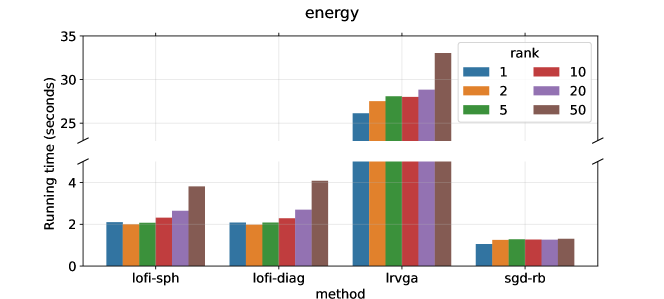
Figure 7: Running time (in seconds) of a single pass over the Energy dataset for various low-rank methods. Figure generated by plots-xval-passes.ipynb

	dataset	Boston	Concrete	Energy	Kin8nm	Naval	Power	Wine	Yacht
rank	variable
0	fdekf	$5.23\pm 2.19$	$8.60\pm 0.63$	$2.96\pm 0.25$	$0.12\pm 0.01$	$0.01\pm 0.00$	$4.24\pm 0.16$	$0.82\pm 0.05$	$5.13\pm 1.30$
1	lofi-sph	$5.08\pm 1.27$	$8.84\pm 1.23$	$3.21\pm 0.36$	$0.14\pm 0.01$	$0.01\pm 0.00$	$4.36\pm 0.15$	$0.67\pm 0.05$	$5.76\pm 1.52$
	lofi-diag	$5.08\pm 1.27$	$9.12\pm 1.35$	$3.50\pm 0.48$	$0.14\pm 0.01$	$0.01\pm 0.00$	$5.01\pm 0.47$	$0.69\pm 0.06$	$5.91\pm 1.52$
	lrvga	$4.14\pm 1.03$	$7.45\pm 0.75$	$2.92\pm 0.22$	$0.14\pm 0.01$	-	$4.25\pm 0.15$	$0.65\pm 0.04$	$5.06\pm 1.06$
	sgd-rb	$4.44\pm 1.20$	$9.62\pm 0.63$	$3.19\pm 0.30$	$0.16\pm 0.01$	$0.01\pm 0.00$	$4.41\pm 0.18$	$0.66\pm 0.04$	$9.84\pm 1.94$
2	lofi-sph	$4.38\pm 1.10$	$8.17\pm 0.90$	$3.07\pm 0.30$	$0.26\pm 0.02$	$0.00\pm 0.00$	$4.33\pm 0.16$	$0.66\pm 0.04$	$5.98\pm 1.45$
	lofi-diag	$5.00\pm 1.71$	$8.54\pm 1.15$	$3.34\pm 0.45$	$0.15\pm 0.01$	$0.00\pm 0.00$	$4.59\pm 0.28$	$0.73\pm 0.07$	$5.65\pm 1.30$
	lrvga	$3.88\pm 1.03$	$7.41\pm 0.90$	$2.87\pm 0.22$	$0.14\pm 0.01$	$0.00\pm 0.00$	$4.24\pm 0.14$	$0.65\pm 0.04$	$4.23\pm 0.91$
	sgd-rb	$4.31\pm 1.20$	$9.13\pm 0.63$	$3.16\pm 0.30$	$0.15\pm 0.01$	$0.01\pm 0.00$	$4.50\pm 0.24$	$0.67\pm 0.05$	$9.03\pm 1.64$
5	lofi-sph	$4.10\pm 1.13$	$7.77\pm 1.02$	$2.83\pm 0.26$	$0.15\pm 0.01$	$0.00\pm 0.00$	$4.24\pm 0.15$	$0.65\pm 0.04$	$5.51\pm 1.22$
	lofi-diag	$4.75\pm 1.30$	$8.46\pm 1.37$	$2.87\pm 0.34$	$0.13\pm 0.01$	$0.00\pm 0.00$	$4.56\pm 0.20$	$0.74\pm 0.07$	$4.30\pm 0.88$
	lrvga	$3.71\pm 1.08$	$6.98\pm 0.57$	$2.86\pm 0.21$	$0.13\pm 0.00$	$0.00\pm 0.00$	$4.23\pm 0.15$	$0.65\pm 0.04$	$3.67\pm 0.84$
	sgd-rb	$4.29\pm 1.20$	$8.72\pm 0.72$	$3.18\pm 0.30$	$0.14\pm 0.01$	$0.01\pm 0.00$	$4.72\pm 0.56$	$0.68\pm 0.05$	$8.36\pm 1.36$
10	lofi-sph	$5.12\pm 1.49$	$7.27\pm 0.89$	$2.36\pm 0.16$	$0.12\pm 0.00$	$0.00\pm 0.00$	$4.20\pm 0.15$	$0.65\pm 0.03$	$4.66\pm 0.83$
	lofi-diag	$4.77\pm 1.20$	$7.33\pm 0.89$	$2.53\pm 0.26$	$0.14\pm 0.01$	$0.00\pm 0.00$	$4.37\pm 0.15$	$0.72\pm 0.06$	$4.66\pm 0.83$
	lrvga	$3.62\pm 1.02$	$7.28\pm 0.73$	$2.80\pm 0.22$	$0.12\pm 0.00$	$0.00\pm 0.00$	$4.22\pm 0.15$	$0.65\pm 0.04$	$3.39\pm 0.79$
	sgd-rb	$4.41\pm 1.23$	$8.46\pm 0.77$	$3.18\pm 0.30$	$0.13\pm 0.01$	$0.00\pm 0.00$	$4.81\pm 0.57$	$0.70\pm 0.06$	$7.92\pm 1.27$
20	lofi-sph	$4.88\pm 1.49$	$6.92\pm 0.60$	$2.11\pm 0.28$	$0.11\pm 0.01$	$0.00\pm 0.00$	$4.23\pm 0.15$	$0.65\pm 0.03$	$4.73\pm 0.99$
	lofi-diag	$4.88\pm 1.49$	$8.03\pm 1.25$	$2.16\pm 0.27$	$0.14\pm 0.01$	$0.00\pm 0.00$	$4.41\pm 0.18$	$0.66\pm 0.04$	$2.37\pm 0.63$
	lrvga	$3.57\pm 1.07$	$6.73\pm 0.60$	$2.80\pm 0.22$	$0.11\pm 0.00$	$0.00\pm 0.00$	$4.24\pm 0.16$	$0.64\pm 0.04$	$2.76\pm 1.08$
	sgd-rb	$4.39\pm 1.18$	$8.26\pm 0.95$	$3.04\pm 0.31$	$0.12\pm 0.01$	$0.00\pm 0.00$	$4.77\pm 0.32$	$0.72\pm 0.06$	$7.42\pm 1.24$
50	lofi-sph	$4.84\pm 1.39$	$6.65\pm 0.54$	$1.72\pm 0.20$	$0.10\pm 0.00$	$0.02\pm 0.00$	$4.20\pm 0.14$	$0.69\pm 0.05$	$2.31\pm 0.54$
	lofi-diag	$4.84\pm 1.39$	$6.70\pm 0.50$	$1.84\pm 0.29$	$0.11\pm 0.00$	$0.00\pm 0.00$	$4.30\pm 0.15$	$0.64\pm 0.04$	$4.85\pm 0.98$
	lrvga	$3.52\pm 1.05$	$6.70\pm 0.58$	$2.79\pm 0.22$	$0.11\pm 0.00$	$0.00\pm 0.00$	$4.21\pm 0.15$	$0.64\pm 0.04$	$3.33\pm 0.81$
	sgd-rb	$4.19\pm 1.18$	$7.71\pm 0.88$	$2.73\pm 0.28$	$0.12\pm 0.01$	$0.00\pm 0.00$	$4.81\pm 0.24$	$0.76\pm 0.05$	$6.62\pm 1.19$
full	fcekf	$4.04\pm 1.07$	$6.45\pm 0.53$	$1.58\pm 0.25$	$0.10\pm 0.00$	$0.00\pm 0.00$	$4.13\pm 0.16$	$0.66\pm 0.04$	$3.14\pm 1.09$

Table 3: RMSE for datasets as a function of method, rank after a single pass over the dataset.

	dataset	Boston	Concrete	Energy	Kin8nm	Naval	Power	Wine	Yacht
rank	variable
0	fdekf	$3.20\pm 0.92$	$6.68\pm 0.51$	$2.32\pm 0.22$	$0.10\pm 0.00$	$0.01\pm 0.00$	$4.18\pm 0.15$	$0.82\pm 0.05$	$1.18\pm 0.36$
1	lofi-sph	$5.60\pm 1.43$	$6.35\pm 0.71$	$1.47\pm 0.15$	$0.10\pm 0.01$	$0.00\pm 0.00$	$4.27\pm 0.17$	$0.66\pm 0.04$	$2.12\pm 0.52$
	lofi-diag	$5.21\pm 1.44$	$6.24\pm 0.53$	$2.22\pm 0.21$	$0.11\pm 0.00$	$0.01\pm 0.00$	$4.17\pm 0.15$	$0.64\pm 0.04$	$1.76\pm 0.43$
	sgd-rb	$3.47\pm 0.98$	$6.57\pm 0.47$	$2.04\pm 0.22$	$0.09\pm 0.00$	$0.00\pm 0.00$	$4.23\pm 0.20$	$0.65\pm 0.04$	$4.82\pm 0.81$
2	lofi-sph	$3.51\pm 0.94$	$6.23\pm 0.64$	$1.16\pm 0.18$	$0.31\pm 0.05$	$0.00\pm 0.00$	$4.20\pm 0.15$	$0.65\pm 0.04$	$2.49\pm 0.51$
	lofi-diag	$5.08\pm 1.43$	$6.19\pm 0.50$	$1.97\pm 0.22$	$0.10\pm 0.00$	$0.00\pm 0.00$	$4.17\pm 0.15$	$0.63\pm 0.04$	$1.75\pm 0.49$
	sgd-rb	$3.50\pm 0.97$	$6.41\pm 0.53$	$1.86\pm 0.19$	$0.09\pm 0.00$	$0.00\pm 0.00$	$4.27\pm 0.22$	$0.65\pm 0.04$	$4.31\pm 0.70$
5	lofi-sph	$3.47\pm 1.00$	$6.02\pm 0.50$	$1.36\pm 0.13$	$0.14\pm 0.02$	$0.00\pm 0.00$	$4.17\pm 0.14$	$0.65\pm 0.04$	$2.44\pm 0.53$
	lofi-diag	$4.95\pm 1.31$	$5.74\pm 0.48$	$1.57\pm 0.19$	$0.10\pm 0.00$	$0.00\pm 0.00$	$4.14\pm 0.15$	$0.63\pm 0.04$	$1.40\pm 0.39$
	sgd-rb	$3.60\pm 0.87$	$6.28\pm 0.61$	$1.51\pm 0.20$	$0.10\pm 0.01$	$0.00\pm 0.00$	$4.45\pm 0.34$	$0.68\pm 0.05$	$3.40\pm 0.61$
10	lofi-sph	$5.38\pm 1.36$	$5.63\pm 0.64$	$0.88\pm 0.14$	$0.10\pm 0.00$	$0.00\pm 0.00$	$4.14\pm 0.16$	$0.64\pm 0.04$	$1.51\pm 0.37$
	lofi-diag	$5.08\pm 1.29$	$5.86\pm 0.50$	$1.36\pm 0.19$	$0.09\pm 0.00$	$0.00\pm 0.00$	$4.13\pm 0.16$	$0.64\pm 0.04$	$2.26\pm 0.52$
	sgd-rb	$3.63\pm 0.84$	$6.29\pm 0.68$	$1.08\pm 0.18$	$0.10\pm 0.01$	$0.00\pm 0.00$	$4.73\pm 0.38$	$0.71\pm 0.05$	$2.26\pm 0.56$
20	lofi-sph	$5.14\pm 1.35$	$5.47\pm 0.67$	$0.75\pm 0.17$	$0.09\pm 0.00$	$0.00\pm 0.00$	$4.18\pm 0.17$	$0.64\pm 0.04$	$1.75\pm 0.42$
	lofi-diag	$5.17\pm 1.34$	$5.54\pm 0.49$	$0.92\pm 0.19$	$0.09\pm 0.00$	$0.00\pm 0.00$	$4.10\pm 0.16$	$0.63\pm 0.04$	$1.23\pm 0.28$
	sgd-rb	$3.60\pm 0.98$	$6.08\pm 0.73$	$0.83\pm 0.12$	$0.10\pm 0.01$	$0.00\pm 0.00$	$4.80\pm 0.33$	$0.77\pm 0.07$	$1.32\pm 0.40$
50	lofi-sph	$5.18\pm 1.39$	$5.35\pm 0.52$	$0.59\pm 0.12$	$0.09\pm 0.00$	$0.02\pm 0.00$	$4.12\pm 0.17$	$0.66\pm 0.05$	$1.03\pm 0.32$
	lofi-diag	$5.20\pm 1.37$	$5.54\pm 0.52$	$0.70\pm 0.12$	$0.09\pm 0.00$	$0.00\pm 0.00$	$4.08\pm 0.17$	$0.64\pm 0.04$	$2.30\pm 0.46$
	sgd-rb	$3.70\pm 1.05$	$5.76\pm 0.85$	$0.64\pm 0.08$	$0.11\pm 0.01$	$0.00\pm 0.00$	$4.96\pm 0.26$	$0.83\pm 0.09$	$0.88\pm 0.29$
full	fcekf	$3.13\pm 0.89$	$5.31\pm 0.48$	$0.62\pm 0.09$	$0.09\pm 0.00$	$0.00\pm 0.00$	$4.05\pm 0.17$	$0.64\pm 0.05$	$1.19\pm 0.27$

Table 4: RMSE for datasets as a function of method, rank after 10 passes over the dataset.

	dataset	Boston	Concrete	Energy	Kin8nm	Naval	Power	Wine	Yacht
rank	variable
0	fdekf	$2.95\pm 0.71$	$6.37\pm 0.52$	$2.11\pm 0.21$	$0.09\pm 0.00$	$0.01\pm 0.00$	$4.14\pm 0.16$	$0.82\pm 0.05$	$0.80\pm 0.26$
1	lofi-sph	$5.70\pm 1.28$	$5.89\pm 0.90$	$0.71\pm 0.11$	$0.09\pm 0.00$	$0.00\pm 0.00$	$4.15\pm 0.16$	$0.66\pm 0.05$	$0.96\pm 0.28$
	lofi-diag	$5.48\pm 1.17$	$5.88\pm 0.47$	$1.96\pm 0.20$	$0.10\pm 0.00$	$0.00\pm 0.00$	$4.15\pm 0.16$	$0.63\pm 0.04$	$1.19\pm 0.28$
	sgd-rb	$3.28\pm 0.85$	$5.70\pm 0.76$	$0.69\pm 0.11$	$0.08\pm 0.00$	$0.00\pm 0.00$	$4.13\pm 0.20$	$0.66\pm 0.05$	$1.33\pm 0.35$
2	lofi-sph	$3.26\pm 0.85$	$5.75\pm 0.74$	$0.61\pm 0.09$	$0.29\pm 0.05$	$0.00\pm 0.00$	$4.13\pm 0.15$	$0.66\pm 0.05$	$1.06\pm 0.28$
	lofi-diag	$5.13\pm 1.10$	$5.81\pm 0.47$	$1.68\pm 0.19$	$0.09\pm 0.00$	$0.00\pm 0.00$	$4.15\pm 0.16$	$0.63\pm 0.04$	$1.30\pm 0.38$
	sgd-rb	$3.27\pm 0.83$	$5.74\pm 0.81$	$0.64\pm 0.08$	$0.09\pm 0.00$	$0.00\pm 0.00$	$4.20\pm 0.24$	$0.69\pm 0.06$	$1.13\pm 0.37$
5	lofi-sph	$3.10\pm 0.84$	$5.82\pm 0.75$	$0.67\pm 0.12$	$0.19\pm 0.09$	$0.00\pm 0.00$	$4.13\pm 0.15$	$0.65\pm 0.05$	$1.05\pm 0.23$
	lofi-diag	$4.92\pm 1.13$	$5.44\pm 0.46$	$1.17\pm 0.17$	$0.10\pm 0.00$	$0.00\pm 0.00$	$4.10\pm 0.17$	$0.63\pm 0.04$	$1.08\pm 0.29$
	sgd-rb	$3.38\pm 0.77$	$6.04\pm 0.87$	$0.58\pm 0.06$	$0.09\pm 0.01$	$0.00\pm 0.00$	$4.36\pm 0.30$	$0.73\pm 0.07$	$0.95\pm 0.32$
10	lofi-sph	$5.29\pm 1.12$	$5.41\pm 0.64$	$0.56\pm 0.07$	$0.09\pm 0.00$	$0.00\pm 0.00$	$4.06\pm 0.17$	$0.66\pm 0.05$	$0.92\pm 0.27$
	lofi-diag	$4.99\pm 1.10$	$5.53\pm 0.50$	$0.86\pm 0.14$	$0.09\pm 0.00$	$0.00\pm 0.00$	$4.10\pm 0.16$	$0.63\pm 0.04$	$1.36\pm 0.33$
	sgd-rb	$3.52\pm 0.68$	$5.78\pm 0.87$	$0.60\pm 0.07$	$0.10\pm 0.01$	$0.00\pm 0.00$	$4.74\pm 0.38$	$0.79\pm 0.08$	$0.81\pm 0.25$
20	lofi-sph	$5.01\pm 1.09$	$5.14\pm 0.69$	$0.56\pm 0.07$	$0.09\pm 0.00$	$0.00\pm 0.00$	$4.12\pm 0.19$	$0.67\pm 0.04$	$1.17\pm 0.23$
	lofi-diag	$5.01\pm 1.10$	$5.35\pm 0.45$	$0.67\pm 0.15$	$0.09\pm 0.00$	$0.00\pm 0.00$	$4.06\pm 0.16$	$0.63\pm 0.04$	$1.03\pm 0.28$
	sgd-rb	$3.76\pm 0.74$	$5.86\pm 0.83$	$0.56\pm 0.06$	$0.10\pm 0.01$	$0.00\pm 0.00$	$4.89\pm 0.54$	$0.85\pm 0.08$	$0.78\pm 0.26$
50	lofi-sph	$5.00\pm 1.12$	$5.09\pm 0.66$	$0.48\pm 0.08$	$0.08\pm 0.00$	$0.02\pm 0.00$	$4.05\pm 0.17$	$0.68\pm 0.06$	$0.93\pm 0.20$
	lofi-diag	$5.01\pm 1.11$	$5.27\pm 0.58$	$0.57\pm 0.08$	$0.09\pm 0.00$	$0.00\pm 0.00$	$4.05\pm 0.17$	$0.65\pm 0.04$	$1.38\pm 0.25$
	sgd-rb	$4.05\pm 1.02$	$5.81\pm 0.65$	$0.53\pm 0.08$	$0.10\pm 0.00$	$0.00\pm 0.00$	$4.73\pm 0.35$	$0.94\pm 0.11$	$0.71\pm 0.38$
full	fcekf	$3.62\pm 1.28$	$5.12\pm 0.59$	$0.52\pm 0.06$	$0.09\pm 0.00$	$0.00\pm 0.00$	$4.00\pm 0.17$	$0.68\pm 0.06$	$1.12\pm 0.29$

Table 5: RMSE for datasets as a function of method, rank after 50 passes over the dataset.

		boston	concrete	energy	kin8nm	naval	power	wine	yacht
rank
1	lofi-sph	$1.93$	$2.17$	$2.10$	$4.31$	$5.39$	$4.60$	$2.40$	$1.96$
	lofi-diag	$2.12$	$2.15$	$2.08$	$4.31$	$6.38$	$4.61$	$2.40$	$1.97$
	lrvga	$31.31$	$31.44$	$26.14$	$194.52$	$819.99$	$125.78$	$69.74$	$13.88$
	sgd-rb	$1.40$	$1.04$	$1.05$	$1.58$	$1.86$	$1.58$	$1.15$	$1.02$
2	lofi-sph	$1.88$	$2.07$	$2.00$	$4.38$	$5.47$	$4.70$	$2.28$	$1.84$
	lofi-diag	$1.91$	$2.04$	$1.98$	$4.34$	$5.43$	$4.68$	$2.27$	$1.85$
	lrvga	$32.83$	$33.90$	$27.53$	$215.47$	$884.71$	$145.94$	$75.78$	$14.30$
	sgd-rb	$1.26$	$1.31$	$1.25$	$2.30$	$2.77$	$2.44$	$2.92$	$1.19$
5	lofi-sph	$1.92$	$2.16$	$2.07$	$4.95$	$6.26$	$5.34$	$2.41$	$3.44$
	lofi-diag	$1.91$	$2.66$	$2.08$	$4.95$	$6.28$	$5.34$	$2.43$	$1.92$
	lrvga	$33.06$	$34.19$	$28.09$	$219.50$	$892.29$	$149.50$	$76.85$	$14.43$
	sgd-rb	$1.26$	$1.28$	$1.28$	$2.27$	$2.81$	$2.39$	$1.42$	$1.20$
10	lofi-sph	$2.13$	$2.89$	$2.31$	$6.17$	$8.51$	$6.65$	$2.66$	$2.00$
	lofi-diag	$2.13$	$2.40$	$2.28$	$6.40$	$8.56$	$7.95$	$2.67$	$1.99$
	lrvga	$32.99$	$33.91$	$28.01$	$218.10$	$888.80$	$151.09$	$75.00$	$14.37$
	sgd-rb	$1.25$	$1.26$	$1.27$	$2.32$	$2.93$	$2.41$	$2.95$	$1.19$
20	lofi-sph	$2.31$	$2.74$	$2.64$	$8.68$	$12.36$	$10.29$	$3.28$	$2.19$
	lofi-diag	$2.31$	$2.74$	$2.70$	$9.34$	$12.30$	$10.30$	$3.25$	$3.89$
	lrvga	$34.19$	$35.90$	$28.84$	$234.75$	$910.09$	$169.94$	$77.88$	$14.92$
	sgd-rb	$1.25$	$1.27$	$1.26$	$2.38$	$2.89$	$2.49$	$1.46$	$1.22$
50	lofi-sph	$3.24$	$4.42$	$3.81$	$19.59$	$39.47$	$21.43$	$5.58$	$2.75$
	lofi-diag	$3.44$	$4.64$	$4.08$	$19.56$	$26.90$	$21.50$	$6.03$	$2.80$
	lrvga	$36.65$	$41.84$	$33.04$	$280.21$	$988.45$	$222.46$	$88.81$	$16.80$
	sgd-rb	$1.25$	$1.35$	$1.31$	$2.77$	$3.52$	$2.97$	$1.52$	$1.24$
full	fcekf	$1.34$	$1.69$	$1.24$	$2.56$	$5.98$	$2.34$	$1.61$	$1.15$

Table 6: Running time (in seconds) for benchmarked methods after a single pass over the UCI datasets.

D.2 Piecewise stationary 1d regression

Figure 8: Results for piecewise stationary 1d regression. Red dots are from the true function for each task, and the blue dots are the predictions of the model at the end of each task (after training on 200 examples). Figure generated by nonstat-1d-regression.ipynb

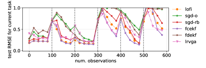
Figure 9: RMSE (rolling average) on test data from the current task for the 1d regression benchmark for different estimators. Vertical lines denote change in the distribution (unknown to the algorithm). Figure generated by nonstat-1d-regression.ipynb

In this section, we consider a synthetic 1d nonstationary regression problem which exhibits “concept drift” (Gama et al., 2014). Specifically we define the data generating process at time $t$ to be $p_{t}(x,y)=p(x)p_{d(t)}(y|x)$, where $p(x)=\mathrm{Unif}(-2,2)$ is the input distribution, $d(t)\in\{1,\ldots,K\}$ specifies which distribution to use at time $t$, and $p_{k}(y|x)=\mathcal{N}(y|f_{k}(x),\sigma^{2})$ is the $k$’th such distribution, for $k=1:K$. We define $f_{k}(x)=x+0.3\sin(w_{k}^{0}+w_{k}^{1}\pi x)$, where ${\bm{w}}_{k}$ are randomly sampled coefficients corresponding to the phase and frequency of the sine wave. We assume $d(t)$ is a staircase function, so $d(t)=k$ for $T_{k-1}\leq t\leq T_{k}$, where $T_{k}-T_{k-1}=250$ is the number of steps before the distribution changes. We visualize these random functions in fig. 8.

Next we fit a one-layer MLP (with 50 hidden units) on this data stream. (The algorithms are unaware of the task boundaries, corresponding to the change in distribution.) The test error (for the current distribution) vs time is shown in fig. 9. The “spikes” in the error rate correspond to times when the distribution changes. In some cases the change in distribution is small (when $f_{t}$ is similar to $f_{t-1}$), but in other cases there is a large shift. The speed with which an estimator can adapt to such changes is a critical performance metric in many domains. We see that FCEKF adapts the fastest, followed by LO-FI and then LRVGA. SGD and the diagonal methods are less sample efficient. However, after a sufficient number of training examples, most methods converge to a good fit, as shown in fig. 8.

D.3 Stationary image classification

In this section we report more results on stationary classification experiments.

In fig. 10(a) we plot the plugin NLL on static fasion MNIST using an MLP with 2 layers with 500 hidden units each, with $648,010$ parameters. The trends are similar to the misclassification rate in fig. 1(a).

In fig. 10(b) we plot the NLPD results using the linearized likelihood and deterministic probit trick discussed in appendix B. We see that in general NLPD outperforms the plugin NLL. Furthermore, the posterior from LOFI outperforms the posterior from the (diagonal) Laplace approximation.

Next we use a CNN, specifically a LeNet-style architecture with 3 hidden layers and 421,641 parameters. The results are shown in fig. 11. The trends are similar to the MLP case, except the gaps in performance among the methods are narrower.

In table 7 we summarize the effects of changing the rank of LO-FI, and of different kinds of inflation (discussed in appendix E), and of switching from diagonal to spherical covariance (discussed in appendix F) on the static fashion-MNIST dataset (using the CNN model) after 500 training examples. Not surprisingly, higher rank improves the results, as does using a diagonal approximation. However, inflation seems to have a negligible effect. In fig. 12, we visualize these differences as a function of sample size.

	spherical				diagonal
	none	bayesian	hybrid	simple	none	bayesian	hybrid	simple
rank
$1$	$42.6$ $\pm$ $0.9$	$42.6$ $\pm$ $0.9$	$42.6$ $\pm$ $0.9$	$41.5$ $\pm$ $1.2$	$41.3$ $\pm$ $1.1$	$40.1$ $\pm$ $1.1$	$40.6$ $\pm$ $1.2$	$40.6$ $\pm$ $1.2$
$5$	$37.5$ $\pm$ $1.1$	$37.8$ $\pm$ $1.1$	$37.6$ $\pm$ $1.1$	$38.0$ $\pm$ $1.1$	$36.6$ $\pm$ $1.3$	$37.0$ $\pm$ $2.0$	$37.0$ $\pm$ $2.0$	$37.0$ $\pm$ $2.0$
$10$	$31.8$ $\pm$ $1.0$	$32.4$ $\pm$ $1.1$	$30.8$ $\pm$ $0.8$	$31.2$ $\pm$ $0.8$	$30.8$ $\pm$ $1.0$	$32.5$ $\pm$ $1.5$	$31.7$ $\pm$ $1.1$	$30.6$ $\pm$ $0.8$
$20$	$31.5$ $\pm$ $1.0$	$35.9$ $\pm$ $1.6$	$30.1$ $\pm$ $0.9$	$30.1$ $\pm$ $0.8$	$28.7$ $\pm$ $0.6$	$31.1$ $\pm$ $1.2$	$32.7$ $\pm$ $0.9$	$32.3$ $\pm$ $1.1$
$50$	$28.0$ $\pm$ $0.7$	$31.7$ $\pm$ $1.3$	$31.7$ $\pm$ $1.3$	$31.7$ $\pm$ $1.3$	$28.6$ $\pm$ $0.8$	$28.4$ $\pm$ $0.7$	$29.1$ $\pm$ $0.6$	$28.4$ $\pm$ $0.7$

Table 7: Stationary fashion-MNIST test set misclassification rates using LO-FI of various ranks after $500$ training examples. We show results for diagonal vs spherical covariance and different forms of inflation (described in appendix E). Means and standard errors computed over $10$ trials.

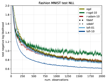
(a)

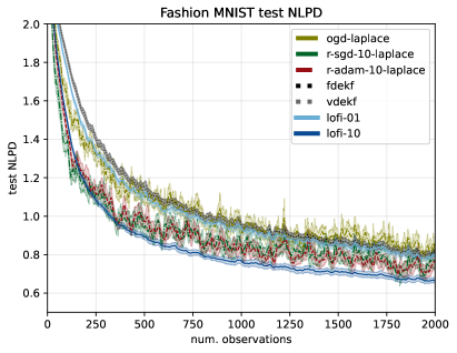
(b)

Figure 10: Test set performance vs number of observations on the fashion-MNIST dataset using MLP. We show the mean and standard errors across random trials. (a) Negative log likelihood ($100$ random trials). (b) NLPD under linearized observation model with probit approximation ($20$ random trials). Figure generated by generate_stationary_clf_plots.ipynb

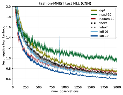
(a)

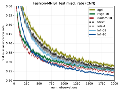
(b)

Figure 11: Test set performance vs number of observations on the fashion-MNIST dataset using a CNN. We show the mean and standard errors across $100$ random trials. (a) Negative log-likelihood. (b) Misclassification rate. Figure generated by generate_stationary_clf_plots.ipynb

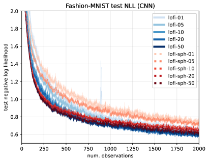
(a)

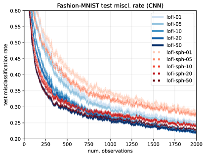
(b)

Figure 12: Results on fashion-MNIST classification dataset using a CNN. We visualize the effect of changing rank, and using diagonal vs spherical LOFI (see appendix F). ”lofi-sph-xx” refers to spherical LO-FI of rank xx (a) negative log-likelihood; (b) misclassification rate. Figure generated by generate_stationary_clf_plots.py

D.4 Piecewise stationary image classification

In this section we report more results on piecewise stationary classification experiments.

Permuted Fashion-MNIST

In fig. 13, we plot the NLL on permuted fashion MNIST. The results are similar to the misclassification rates in fig. 1(c), except now the gap between LOFI and the other methods is even larger. In fig. 14 we compare the test-set misclassification rates of LO-FI of various ranks. We see that performance improves with rank and plateaus at about rank 10.

In fig. 15, we show the test-set predictions (plugin approxmation) from a LO-FI-10 estimator on a sample image from each of the first five tasks at various points during training. Before the model has seen data from a given distribution (yellow panels), its predictions are mostly uniform; once it encounters data from the distribution, it learns rapidly, as can be seen by the red NLL bar going down (the model is less surprised when it sees the true label); after the distribution shifts, we can still assess its performance on past tasks (gray panels), and we see that the model is fairly good at remembering the past. At the bottom of the plot, we show predictions on an OOD dataset that the model is never trained on; we see that predictions remain close to uniform, indicating high uncertainty. In fig. 16, we show the same results using RSGD estimator; we see that it is much less entropic, even when it should be uncertain (e.g. for OOD).

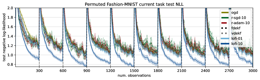
Figure 13: Non-stationary permuted fashion-MNIST classification. The task boundaries are denoted by vertical lines. We report NLL performance on the current task’s test set. Figure generated by generate_permuted_clf_plots.ipynb

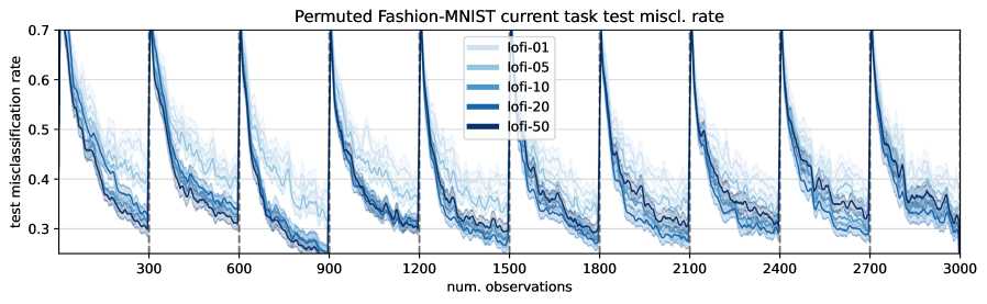
Figure 14: Test set misclassification rates vs number of observations on the permuted fashion-MNIST dataset. We compare the performance as a function of the rank of LO-FI. Figure generated by generate_permuted_clf_plots.ipynb.

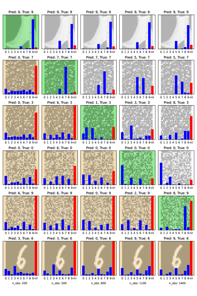
Figure 15: Test set predictions for non-stationary permuted fashion-MNIST classification problem using LO-FI rank 10. Rows correspond to different distributions / tasks (i.e., different permutations of the data), and columns represent snapshots of the posterior predictive after every 50 steps of online learning. Thus we can assess the performance of the model after seeing tasks $1:t$ by looking at the $t$’th column, and reading down across the rows. The first task uses the identity permutation. The last row corresponds to an out-of-distribution example taken from the MNIST dataset. The current task is shown in green; previously seen tasks are shown in gray, and future tasks are shown in yellow. The blue bars are the predicted class probabilities (using plugin estimate), and the red bar is the NLL of the true label. in red. Figure generated by probe.ipynb

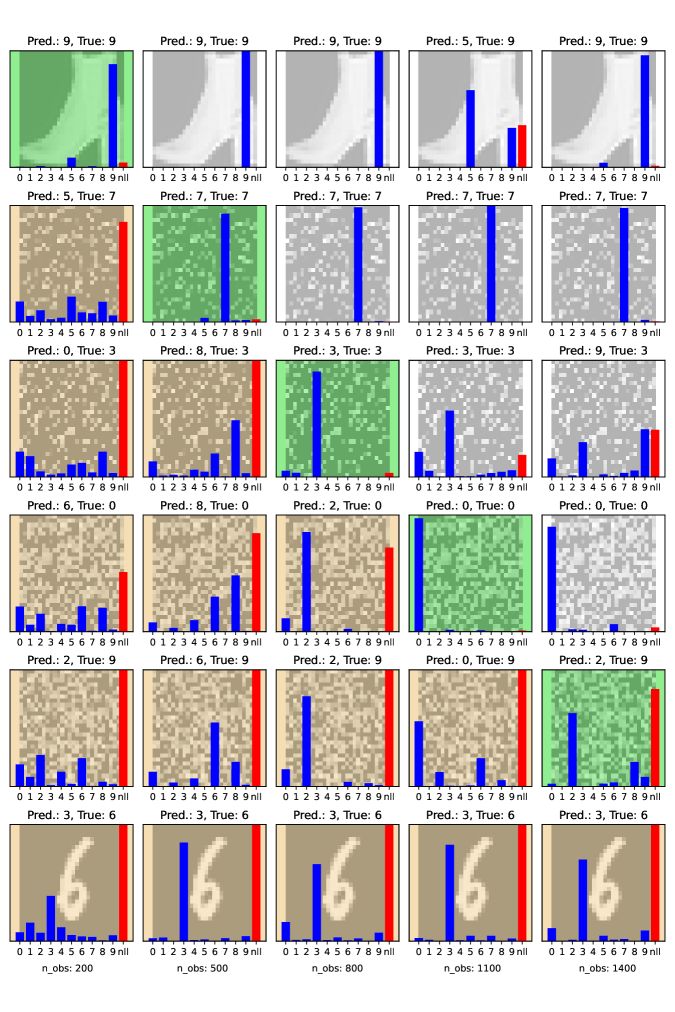
Figure 16: Same as fig. 15 except using replay-SGD estimator.

Split Fashion-MNIST

In fig. 17, we evaluate the methods using the split fashion-MNIST dataset. This task seems so easy that we cannot detect any substantial difference in test-set performance among the different methods.

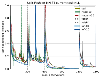
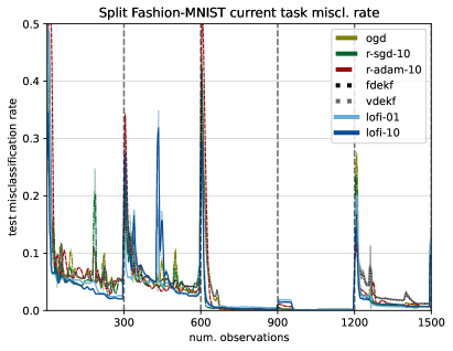
Figure 17: Test set performance vs number of observations on the split fashion-MNIST dataset. (a) negative log-likelihood; (b) misclassification rate. Figure generated by generate_split_clf_plots.ipynb.

D.5 Slowly changing image classification

In fig. 18 we plot NLL and NLPD for the gradually rotating fashion-MNIST experiment. The difference between the methods is more visible when judged by NLL compared to the misclassification error in fig. 1(b). We see that LO-FI outperforms other methods.

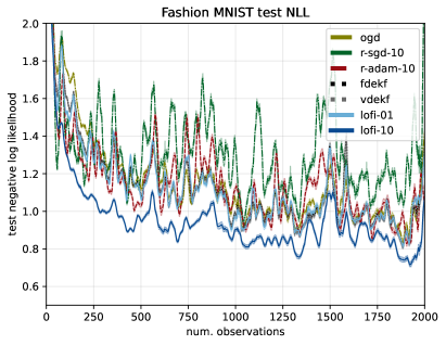
(a)

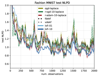
(b)

Figure 18: Gradually rotating fashion-MNIST classification. We evaluate the performance on a test set from the current distribution (within a window). (a) NLL. (b) NLPD under probit approximation. Figure generated by generate_rotated_clf_plots.ipynb.

D.6 Stationary image regression

In fig. 19(a) we show the NLL (per example) for the static fashion-MNIST regression problem. This has the same shape as the RMSE results in fig. 2(a), since NLL = RMSE + constant, since we assume the observation noise is fixed.

In fig. 19(b) we show the NLPD for the same problem, which is approximated using the posterior predictive distribution under the linearized observation model (see appendix B). We see that the NLPD metric of each method outperforms its respective NLL metric, and the variance is much lower. We also see that the posterior from LOFI outperforms the posterior from (diagonal) Laplace.

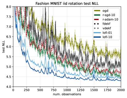
(a)

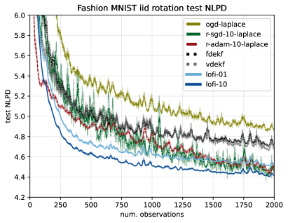
(b)

Figure 19: IID rotated fashion-MNIST regression problem. (a) NLL using MAP plug-in estimate. (b) NLPD under linearized observation model. Figure generated by generate_iid_reg_plots.ipynb

D.7 Piecewise stationary image regression

In fig. 20 we show results for a piecewise stationary distribution created by using permuted fashion MNIST with $300$ samples per task to create $10$ tasks. We see that LO-FI outperforms RSGD by a large margin.

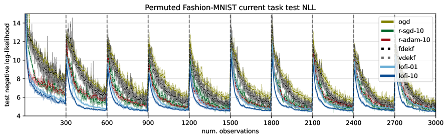
(a)

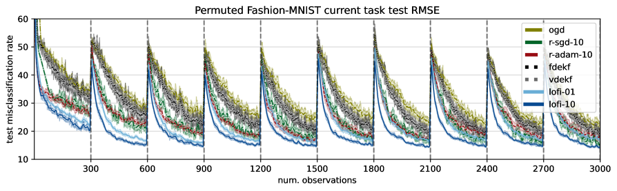
(b)

Figure 20: Permuted rotating Fashion MNIST regression problem using MAP plugin prediction. (a) Negative log-likelihood; (b) RMSE. Figure generated by generate_permuted_reg_plots.ipynb

D.8 Slowly changing image regression

In fig. 21(b) we show the linearized approximation to the NLPD on the drifting MNIST rotation regression problem. Note that under the nonstationary setting, the GD-based methods are extremely noisy, whereas LO-FI is much more stable.

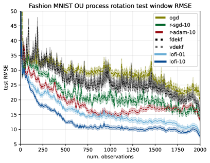
(a)

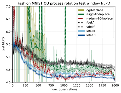
(b)

Figure 21: Slowly drifting MNIST regression problem. (a) RMSE using MAP estimate. (b) NLPD using linearized likelihood. Figure generated by generate_rw_reg_plots.ipynb

D.9 Bandits

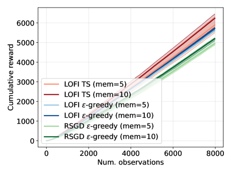
Figure 22: Reward vs time on MNIST bandit problem. We show results (averaged over 5 trials) using Thompson sampling or $\epsilon$-greedy with $\epsilon=0.1$. Figure generated by bandit-vs-memory.ipynb

In fig. 22 we show reward vs time for different methods on the MNIST bandit problem. We see that LOFI with Thompson sampling beats LOFI with $\epsilon$-greedy, which beats replay SGD with $\epsilon$-greedy.

D.10 LRVGA implementation

The orignal numpy code for LRVGA code is at https://github.com/marc-h-lambert/L-RVGA. We reimeplemented it in JAX and verified that it gives the same results when applied to their linear regression examples. Specifically we used their source code with initial hyperparameters $\sigma^{2}_{0}=1$ and $\epsilon=10^{-3}$. In fig. 23, we visually compare the KL between our posterior and theirs, verifying that our implementation is correct. By using JAX, we gain speed. More importantly we can extend the method to the nonlinear case by using JAX’s autodiff framework to compute the relevant gradients.

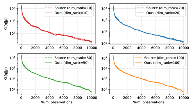
Figure 23: KL divergence comparison between the original LRVGA implementation (source) and our implementation. Figure generated by xp-lrvga-linear-regression.ipynb

Appendix E Covariance inflation

In this section we derive a modified version of LO-FI where we use a Bayesian version of the covariance inflation trick of (Ollivier, 2018; Alessandri et al., 2007; Kurle et al., 2020) to account for errors introduced by approximate inference, such as linearizing the observation model (see (Kulhavý & Zarrop, 1993; Kárný, 2014) for analysis). In practice this just requires a rescaling of the terms in the posterior precision matrix at the end of each update step (or equivalently, just before doing a predict step). This rescaling only takes $O(P)$ time, so is negligible extra cost. However, we have found it does not seem to improve results (see table 7 for results on UCI regression); thus this section is just for “historical interest”.

Section E.1 derives our Bayesian inflation method, in which discounting is applied only to the likelihood and not to the prior. This amounts to deflating the entire log posterior and then adding back in the appropriate fraction of the log prior. Section E.2 derives a simpler version of inflation that discounts the entire posterior (i.e., likelihood and prior), matching past work (Alessandri et al., 2007; Ollivier, 2018). Section E.3 derives a hybrid inflation method that uses the covariance update from Bayesian inflation but, like simple inflation, does not change the mean. This turns out to be a special case of the regularized forgetting mechanism of Kulhavý & Zarrop (1993), which they derive based on uncertainty about the system dynamics rather than drift in the observation model.

We derive all three variations for a general state-space model and then show how they specialize to LO-FI. The results are formulas for going from the parameters of the posterior after step $t-1$ ($\bm{\mu}_{t-1},\bm{\Upsilon}_{t-1},\mathbf{W}_{t-1}$) to parameters of an “inflated” posterior ($\acute{\bm{\mu}}_{t-1},\acute{\bm{\Upsilon}}_{t-1},\acute{\mathbf{W}}_{t-1}$). Applying inflation then amounts to substituting $\acute{\bm{\mu}}_{t-1},\acute{\bm{\Upsilon}}_{t-1},\acute{\mathbf{W}}_{t-1}$ for ${\bm{\mu}}_{t-1},{\bm{\Upsilon}}_{t-1},{\mathbf{W}}_{t-1}$ in eqs. 15, 19 and 25 in section A.1.

E.1 Bayesian inflation

Consider first the special case of a static parameter ($\forall_{t}:{\bm{\theta}}_{t}={\bm{\theta}}_{0}$). The log posterior after step $t-1$ is

$$\log p({\bm{\theta}}|{\mathcal{D}}_{1:t-1})=\log p({\bm{\theta}})+\sum_{i=1}^{t-1}\log p({\bm{y}}_{i}|{\bm{x}}_{i},{\bm{\theta}})+const$$ (69)

We modify this expression by discounting the likelihood of each past observation by $(1+\alpha)^{-k}$, where $k=t-1-i$ is the lag. For Gaussian observations, this is equivalent to scaling up the observation covariance $\mathbf{R}_{i}$ by $(1+\alpha)^{-k}$. We indicate this discounting by the subscripted probability $p_{t-1}$, where time $t-1$ is the reference point from which discounting is applied.

$$\log p_{t-1}({\bm{\theta}}|{\mathcal{D}}_{1:t-1})=\log p({\bm{\theta}})+\sum_{i=1}^{t-1}(1+\alpha)^{-(t-1-i)}\log p({\bm{y}}_{i}|{\bm{x}}_{i},{\bm{\theta}})+const$$ (70)

Passing from $p_{t-1}$ to $p_{t}$ amounts to applying an additional discount factor to the likelihoods, which is equivalent to discounting the entire log posterior and adding back a fraction of the log prior so that it is not discounted:

$$\log p_{t}({\bm{\theta}}|{\mathcal{D}}_{1:t-1}) =\log p({\bm{\theta}})+\sum_{i=1}^{t-1}(1+\alpha)^{-(t-i)}\log p({\bm{y}}_{i}|{\bm{x}}_{i},{\bm{\theta}})+const$$ (71)

$$=\log p({\bm{\theta}})+\frac{1}{1+\alpha}\sum_{i=1}^{t-1}(1+\alpha)^{-(t-1-i)}\log p({\bm{y}}_{i}|{\bm{x}}_{i},{\bm{\theta}})+const$$ (72)

$$=\frac{1}{1+\alpha}\log p_{t-1}({\bm{\theta}}|{\mathcal{D}}_{1:t-1})+\frac{\alpha}{1+\alpha}\log p({\bm{\theta}})$$ (73)

The same reasoning applies in the general case with state dynamics. We expand the log posterior after step $t-1$ as

$$\log p_{t-1}({\bm{\theta}}_{t-1}|{\mathcal{D}}_{1:t-1})=\log p({\bm{\theta}}_{t-1})+\log p_{t-1}({\mathcal{D}}_{1:t-1}|{\bm{\theta}}_{t-1})+const$$ (74)

Passing from $p_{t-1}$ to $p_{t}$ amounts to discounting the data contribution while preserving the latent predictive prior:

$$\log p_{t}({\bm{\theta}}_{t-1}|{\mathcal{D}}_{1:t-1}) =\log p({\bm{\theta}}_{t-1})+\frac{1}{1+\alpha}\log p_{t-1}({\mathcal{D}}_{1:t-1}|{\bm{\theta}}_{t-1})+const$$ (75)

$$=\frac{1}{1+\alpha}\log p_{t-1}({\bm{\theta}}_{t-1}|{\mathcal{D}}_{1:t-1})+\frac{\alpha}{1+\alpha}\log p({\bm{\theta}}_{t-1})+const$$ (76)

A similar result was derived in (Kurle et al., 2020).

We now specialize eq. 76 to LO-FI. Given our initial prior $p({\bm{\theta}}_{0})=\mathcal{N}({\bm{\theta}}_{0}|\bm{\mu}_{0},\eta_{0}^{-1}\mathbf{I}_{P})$ and dynamics $p({\bm{\theta}}_{t}|{\bm{\theta}}_{t-1})=\mathcal{N}({\bm{\theta}}_{t}|\gamma_{t}{\bm{\theta}}_{t-1},q_{t}\mathbf{I}_{P})$, the latent unconditional predictive prior of the dynamical system at time $t-1$ is

$$p({\bm{\theta}}_{t-1}) =\mathcal{N}({\bm{\theta}}_{t-1}|\Gamma_{t-1}\bm{\mu}_{0},\eta_{t-1}^{-1}\mathbf{I}_{P})$$ (77)

$$\eta_{t}^{-1} =\gamma_{t}^{2}\eta_{t-1}^{-1}+q_{t}$$ (78)

$$\Gamma_{t-1} =\prod_{i=1}^{t-1}\gamma_{i}$$ (79)

Substituting this and our posterior $p_{t-1}({\bm{\theta}}_{t-1}|{\mathcal{D}}_{1:t-1})=\mathcal{N}({\bm{\theta}}_{t-1}|\bm{\mu}_{t-1},(\bm{\Upsilon}_{t-1}+\mathbf{W}_{t-1}\mathbf{W}_{t-1}^{\mkern-1.5mu\mathsf{T}})^{-1})$ into eq. 76 yields

$$p_{t}({\bm{\theta}}_{t-1}|{\mathcal{D}}_{1:t-1})=\mathcal{N}\left({\bm{\theta}}_{t-1}\middle|\acute{\bm{\mu}}_{t-1},\left(\acute{\bm{\Upsilon}}_{t-1}+\acute{\mathbf{W}}_{t-1}\acute{\mathbf{W}}_{t-1}^{\mkern-1.5mu\mathsf{T}}\right)^{-1}\right)$$ (80)

with

$$\acute{\bm{\mu}}_{t-1} =\bm{\mu}_{t-1}+\frac{\alpha\eta_{t-1}}{1+\alpha}\left(\acute{\bm{\Upsilon}}_{t-1}+\acute{\mathbf{W}}_{t-1}\acute{\mathbf{W}}_{t-1}^{\mkern-1.5mu\mathsf{T}}\right)^{-1}(\Gamma_{t-1}\bm{\mu}_{0}-\bm{\mu}_{t-1})$$ (81)

$$\acute{\bm{\Upsilon}}_{t-1} =\frac{1}{1+\alpha}\bm{\Upsilon}_{t-1}+\frac{\alpha\eta_{t-1}}{1+\alpha}\mathbf{I}_{P}$$ (82)

$$\acute{\mathbf{W}}_{t-1} =\frac{1}{\sqrt{1+\alpha}}\mathbf{W}_{t-1}$$ (83)

Equation 81 implements a form of regularization toward the prior predictive mean $\Gamma_{t-1}\bm{\mu}_{0}$, which originates in the log-prior term in eq. 76. Equations 82 and 83 implement inflation of the covariance by a factor of $1+\alpha$, together with the log-prior correction being added to $\acute{\bm{\Upsilon}}_{t-1}$. Together these expressions show how the parameters of the distribution change as we pass from $p_{t-1}({\bm{\theta}}_{t-1}|{\mathcal{D}}_{1:t-1})$ to $p_{t}({\bm{\theta}}_{t-1}|{\mathcal{D}}_{1:t-1})$. Notice that we have incremented the subscript in $p_{t}$ but the random variable is still ${\bm{\theta}}_{t-1}$. Thus $\acute{\bm{\mu}}_{t-1},\acute{\bm{\Upsilon}}_{t-1},\acute{\mathbf{W}}_{t-1}$ define the “post-inflation” posterior that is passed to the predict step in section A.1 to obtain the iterative prior, given by $\bm{\mu}_{t|t-1},\bm{\Upsilon}_{t|t-1},\mathbf{W}_{t|t-1}$.

E.2 Simple inflation

A simpler version of inflation can be obtained by discounting the prior as well as the likelihood. In that case, passing from $p_{t-1}$ to $p_{t}$ amounts to discounting the entire log posterior. Thus instead of eq. 76 we have

$$\log p_{t}({\bm{\theta}}_{t-1}|{\mathcal{D}}_{1:t-1}) =\frac{1}{1+\alpha}\log p_{t-1}({\bm{\theta}}_{t-1}|{\mathcal{D}}_{1:t-1})$$ (84)

Substituting $p_{t-1}({\bm{\theta}}_{t-1}|{\mathcal{D}}_{1:t-1})=\mathcal{N}({\bm{\theta}}_{t-1}|\bm{\mu}_{t-1},(\bm{\Upsilon}_{t-1}+\mathbf{W}_{t-1}\mathbf{W}_{t-1}^{\mkern-1.5mu\mathsf{T}})^{-1})$ yields

$$p_{t}({\bm{\theta}}_{t-1}|{\mathcal{D}}_{1:t-1}) =\mathcal{N}\left({\bm{\theta}}_{t-1}\middle|\bm{\mu}_{t-1},(1+\alpha)\left(\bm{\Upsilon}_{t-1}+\mathbf{W}_{t-1}\mathbf{W}_{t-1}^{\mkern-1.5mu\mathsf{T}}\right)^{-1}\right)$$ (85)

Thus we merely inflate the covariance by $1+\alpha$, as in Alessandri et al. (2007) and Ollivier (2018). This implies the simple inflation equations

$$\acute{\bm{\mu}}_{t-1} =\bm{\mu}_{t-1}$$ (86)

$$\acute{\bm{\Upsilon}}_{t-1} =\frac{1}{1+\alpha}\bm{\Upsilon}_{t-1}$$ (87)

$$\acute{\mathbf{W}}_{t-1} =\frac{1}{\sqrt{1+\alpha}}\mathbf{W}_{t-1}$$ (88)

E.3 Hybrid inflation

Rather than mixing in the latent predictive prior, as in eq. 76, we can mix in a distribution that uses the prior predictive variance but the posterior mean:

$$\log p_{t}({\bm{\theta}}_{t-1}|{\mathcal{D}}_{1:t-1}) =\frac{1}{1+\alpha}\log p_{t-1}({\bm{\theta}}_{t-1}|{\mathcal{D}}_{1:t-1})+\frac{\alpha}{1+\alpha}\log\mathcal{N}({\bm{\theta}}_{t-1}|\bm{\mu}_{t-1},\eta_{t-1}^{-1}\mathbf{I}_{P})+const$$ (89)

This approach fits into the more general regularized forgetting framework of Kulhavý & Zarrop (1993) and can be interpreted heuristically as regularizing the covariance but not the mean, which may be preferable since $\bm{\mu}_{0}$ is sampled randomly rather than being an informed prior. In this case, substituting LO-FI’s posterior $p_{t-1}({\bm{\theta}}_{t-1}|{\mathcal{D}}_{1:t-1})=\mathcal{N}({\bm{\theta}}_{t-1}|\bm{\mu}_{t-1},(\bm{\Upsilon}_{t-1}+\mathbf{W}_{t-1}\mathbf{W}_{t-1}^{\mkern-1.5mu\mathsf{T}})^{-1})$ yields

$$p_{t}({\bm{\theta}}_{t-1}|{\mathcal{D}}_{1:t-1})=\mathcal{N}\left({\bm{\theta}}_{t-1}\middle|\bm{\mu}_{t-1},(1+\alpha)\left(\bm{\Upsilon}_{t-1}+\alpha\eta_{t-1}\mathbf{I}_{P}+\mathbf{W}_{t-1}\mathbf{W}_{t-1}^{\mkern-1.5mu\mathsf{T}}\right)^{-1}\right)$$ (90)

implying

$$\acute{\bm{\mu}}_{t-1} =\bm{\mu}_{t-1}$$ (91)

$$\acute{\bm{\Upsilon}}_{t-1} =\frac{1}{1+\alpha}\bm{\Upsilon}_{t-1}+\frac{\alpha\eta_{t-1}}{1+\alpha}\mathbf{I}_{P}$$ (92)

$$\acute{\mathbf{W}}_{t-1} =\frac{1}{\sqrt{1+\alpha}}\mathbf{W}_{t-1}$$ (93)

Appendix F Spherical LO-FI

Here we describe a restricted version of LO-FI in which the diagonal part of the precision is isotropic, $\bm{\Upsilon}_{t}=\eta_{t}\mathbf{I}_{P}$. We denote this class of spherical plus low-rank models by SPL($L$), and refer to this algorithm as spherical LO-FI, in contrast to the diagonal LO-FI presented in the main text. Perhaps surprisingly, we find that the spherical restriction can slightly help predictive performance (see UCI regression results in table 3), which is consistent with the claims in (Tomczak et al., 2020). However, the gains are not consistent across datasets.

The spherical restriction also allows a more efficient predict step, taking $O(P)$ instead of $O(PL^{2})$ as in diagonal LO-FI, although in practice the running times are indistinguishable (see fig. 7). The update step takes $O(P\tilde{L}^{2})$, matching diagonal LO-FI, although we present an alternative approximate method in section F.5.2 that takes only $O(PLC)$.

F.1 Warmup

To motivate our approach, consider the case of stationary parameters, where $p({\bm{\theta}}_{t}|{\bm{\theta}}_{t-1})=\delta({\bm{\theta}}_{t}-{\bm{\theta}}_{t-1})$. Then $\bm{\Sigma}_{t|t-1}=\bm{\Sigma}_{t-1}$ and hence eq. 26 becomes $\bm{\Sigma}_{t}^{-1}=\bm{\Sigma}_{t-1}^{-1}+\mathbf{H}_{t}^{\mkern-1.5mu\mathsf{T}}\mathbf{R}_{t}^{-1}\mathbf{H}_{t}$. Hence we can unwind eq. 26 to get

$$\bm{\Sigma}_{t}^{-1}=\eta_{0}\mathbf{I}_{P}+\sum_{i=1}^{t}\mathbf{G}_{i}\mathbf{G}_{i}^{\mkern-1.5mu\mathsf{T}}$$ (94)

where $\mathbf{G}_{t}=\mathbf{H}_{t}^{\mkern-1.5mu\mathsf{T}}\mathbf{A}_{t}^{\mkern-1.5mu\mathsf{T}}\in^{P\times C}$ is the transposed Jacobian of the standardized observation vector $\mathbf{A}_{t}{\bm{y}}_{t}$. The data-driven part of eq. 94 is a sum of outer products of gradients, taken over all time steps and (standardized) outcome dimensions. We seek a low-rank approximation of this sum,

$$\mathbf{W}_{t}\mathbf{W}_{t}^{\mkern-1.5mu\mathsf{T}}\approx\sum_{i=1}^{t}\mathbf{G}_{i}\mathbf{G}_{i}^{\mkern-1.5mu\mathsf{T}}$$ (95)

with $\mathbf{W}_{t}\in^{P\times L}$. LO-FI’s update step uses incremental SVD after each observation to maintain $\mathbf{W}_{t}$ as an approximation of the top $L$ non-normalized singular vectors of $[\mathbf{G}_{1},\dots,\mathbf{G}_{t}]$. Section F.5 describes two alternative versions of incremental SVD, one matching that of diagonal LO-FI (section F.5.1) and the other using a more efficient projection approximation (section F.5.2). In both cases we will have $\mathbf{W}_{t}=\mathbf{U}_{t}\bm{\Lambda}_{t}$, where $\bm{\Lambda}_{t}=\mathrm{diag}(\bm{\lambda}_{t})$ is a diagonal $L\times L$ matrix, and $\mathbf{U}_{t}^{\mkern-1.5mu\mathsf{T}}\mathbf{U}_{t}=\mathbf{I}_{L}$. Therefore the approximate posterior is written as

$$p({\bm{\theta}}_{t}|{\mathcal{D}}_{1:t})=\mathcal{N}\left({\bm{\theta}}_{t}\middle|\bm{\mu}_{t},\left(\eta_{t}\mathbf{I}_{P}+\mathbf{U}_{t}\bm{\Lambda}_{t}^{2}\mathbf{U}_{t}^{\mkern-1.5mu\mathsf{T}}\right)^{-1}\right)$$ (96)

Unlike in diagonal LO-FI, the spherical part of the precision is data-independent. This is because any data-driven update, like eq. 41, would make it nonspherical. Therefore $\eta$ evolves only due to the dynamics in our generative model, eq. 14.

F.2 Steady-state assumption

We find it helpful to make the steady-state assumption that $\mathbb{V}\left[{{\bm{\theta}}_{t}}\right]=\mathbb{V}\left[{{\bm{\theta}}_{0}}\right]$ for all $t$, which is the same as the “variance preserving” OU process used in diffusion probabilistic models (Song et al., 2021; Ho et al., 2020). Because $\mathbb{V}\left[{{\bm{\theta}}_{0}}\right]=\eta_{0}^{-1}\mathbf{I}_{P}$, and because $\mathbb{V}\left[{{\bm{\theta}}_{t}}\right]$ and $\eta_{t}^{-1}$ both evolve according to eq. 14, $\eta_{t}^{-1}=\gamma_{t}^{2}\eta_{t-1}^{-1}+q_{t}$, we have by induction that $\mathbb{V}\left[{{\bm{\theta}}_{t}}\right]=\eta_{t}^{-1}\mathbf{I}_{P}$ for all $t$. Therefore the steady-state assumption is equivalent to $\eta_{t}=\eta_{0}$ and implies the following constraint for all $t$:

$$\gamma_{t}^{2}+q_{t}\eta_{t-1}=1$$ (97)

F.3 Notation

We use $\overline{\square}$ and $\tilde{\square}$ to denote objects whose “focal” dimension is grown from $L$ to $P$ and $\tilde{L}$, respectively. For example, $\mathbf{U}_{t}$ has size $P\times L$ while $\overline{\mathbf{U}}_{t}$ has size $P\times P$ (see eqs. 100 and 101), and $\bm{\Lambda}_{t}$ has size $L\times L$ while $\tilde{\bm{\Lambda}}_{t}$ has size $P\times\tilde{L}$ (with $\tilde{L}$ nonzero entries; see eqs. 39 and 117).

F.4 Predict step for the parameters

The predict step for the parameters, $p({\bm{\theta}}_{t}|{\mathcal{D}}_{1:t-1})=\mathcal{N}({\bm{\theta}}_{t-1}|\bm{\mu}_{t|t-1},\bm{\Sigma}_{t|t-1})$, just requires pushing the previous posterior through the linear-Gaussian dynamics model in eq. 14:

$$\bm{\mu}_{t|t-1} =\gamma_{t}\bm{\mu}_{t-1}$$ (98)

$$\bm{\Sigma}_{t|t-1} =\gamma_{t}^{2}\bm{\Sigma}_{t-1}+q_{t}\mathbf{I}_{P}$$ (99)

To efficiently compute $\bm{\Sigma}_{t-1}$, let $\overline{\mathbf{U}}_{t-1}$ be an orthonormal matrix extending $\mathbf{U}_{t-1}$ from $P\times L$ to $P\times P$, and let $\overline{\bm{\lambda}}_{t-1}\in^{P}$ be a vector extending $\bm{\lambda}_{t-1}$ with zeros:

$$\overline{\mathbf{U}}_{t-1}\overline{\mathbf{U}}_{t-1}^{\mkern-1.5mu\mathsf{T}} =\mathbf{I}_{P}$$ (100)

$$\overline{\mathbf{U}}_{t-1}[:,1{:}L] =\mathbf{U}_{t-1}$$ (101)

$$\overline{\bm{\lambda}}_{t-1}[1{:}L] =\bm{\lambda}_{t-1}$$ (102)

$$\overline{\bm{\lambda}}_{t-1}[(L+1){:}P] =\bm{0}$$ (103)

Then we can diagonalize using $\overline{\mathbf{U}}_{t-1}$:

$$\bm{\Sigma}_{t-1} =\left(\eta_{t-1}\mathbf{I}_{P}+\mathbf{U}_{t-1}\bm{\Lambda}_{t-1}^{2}\mathbf{U}_{t-1}^{{\mkern-1.5mu\mathsf{T}}}\right)^{-1}$$ (104)

$$=\left(\overline{\mathbf{U}}_{t-1}\mathrm{diag}\left(\eta_{t-1}+\overline{\bm{\lambda}}_{t-1}^{2}\right)\overline{\mathbf{U}}_{t-1}^{{\mkern-1.5mu\mathsf{T}}}\right)^{-1}$$ (105)

$$=\overline{\mathbf{U}}_{t-1}\mathrm{diag}\left(\eta_{t-1}+\overline{\bm{\lambda}}_{t-1}^{2}\right)^{-1}\overline{\mathbf{U}}_{t-1}^{{\mkern-1.5mu\mathsf{T}}}$$ (106)

Substituting into eq. 99 gives an efficient expression for the precision:

$$\bm{\Sigma}_{t|t-1}^{-1} =\left(\gamma_{t}^{2}\overline{\mathbf{U}}_{t-1}\mathrm{diag}\left(\eta_{t-1}+\overline{\bm{\lambda}}_{t-1}^{2}\right)^{-1}\overline{\mathbf{U}}_{t-1}^{{\mkern-1.5mu\mathsf{T}}}+q_{t}\mathbf{I}_{P}\right)^{-1}$$ (107)

$$=\overline{\mathbf{U}}_{t-1}\mathrm{diag}\left(\frac{\eta_{t-1}+\overline{\bm{\lambda}}_{t-1}^{2}}{\gamma_{t}^{2}+q_{t}\eta_{t-1}+q_{t}\overline{\bm{\lambda}}_{t-1}^{2}}\right)\overline{\mathbf{U}}_{t-1}^{{\mkern-1.5mu\mathsf{T}}}$$ (108)

$$=\frac{\eta_{t-1}}{\gamma_{t}^{2}+q_{t}\eta_{t-1}}\mathbf{I}_{P}+\mathbf{U}_{t-1}\mathrm{diag}\left(\frac{\gamma_{t}^{2}\bm{\lambda}_{t-1}^{2}}{(\gamma_{t}^{2}+q_{t}\eta_{t-1})(\gamma_{t}^{2}+q_{t}\eta_{t-1}+q_{t}\bm{\lambda}_{t-1}^{2})}\right)\mathbf{U}_{t-1}^{{\mkern-1.5mu\mathsf{T}}}$$ (109)

This implies the updates

$$\eta_{t} =\frac{\eta_{t-1}}{\gamma_{t}^{2}+q_{t}\eta_{t-1}}$$ (110)

$$\bm{\lambda}_{t|t-1}^{2} =\frac{\gamma_{t}^{2}\bm{\lambda}_{t-1}^{2}}{(\gamma_{t}^{2}+q_{t}\eta_{t-1})(\gamma_{t}^{2}+q_{t}\eta_{t-1}+q_{t}\bm{\lambda}_{t-1}^{2})}$$ (111)

$$\mathbf{U}_{t|t-1} =\mathbf{U}_{t-1}$$ (112)

Under the steady-state assumption, eq. 97, these reduce to

$$\eta_{t} =\eta_{t-1}$$ (113)

$$\bm{\lambda}_{t|t-1}^{2} =\frac{\gamma_{t}^{2}\bm{\lambda}_{t-1}^{2}}{1+q_{t}\bm{\lambda}_{t-1}^{2}}$$ (114)

$$\mathbf{U}_{t|t-1} =\mathbf{U}_{t-1}$$ (115)

See algorithm 6 for the pseudocode.

1def $\text{predict}(\bm{\mu}_{t-1},\bm{\lambda}_{t-1},\mathbf{U}_{t-1},\eta_{t-1},{\bm{x}}_{t},\gamma_{t},q_{t})$:

2 $\bm{\mu}_{t|t-1}=\gamma\bm{\mu}_{t-1}$

3 $\bm{\lambda}_{t|t-1}=\sqrt{\frac{\gamma_{t}^{2}\bm{\lambda}_{t-1}^{2}}{(\gamma_{t}^{2}+q_{t}\eta_{t-1})(\gamma_{t}^{2}+q_{t}\eta_{t-1}+q_{t}\bm{\lambda}_{t-1}^{2})}}$ // componentwise

4 $\mathbf{U}_{t|t-1}=\mathbf{U}_{t-1}$

5 $\eta_{t}=\frac{\eta_{t-1}}{\gamma_{t}^{2}+q_{t}\eta_{t-1}}$

6 $\hat{{\bm{y}}}_{t}=h({\bm{x}}_{t},\bm{\mu}_{t|t-1})$

Return $(\hat{{\bm{y}}}_{t},\bm{\mu}_{t|t-1},\bm{\lambda}_{t|t-1},\mathbf{U}_{t|t-1},\eta_{t})$

Algorithm 6 LO-FI predict step (spherical).

F.5 Update step

Algorithm 7 shows the pseudocode for spherical LO-FI’s update step. The mean update is the same as for diagonal LO-FI, eq. 38. Substituting the spherical part of the precision, $\bm{\Upsilon}_{t|t-1}=\eta_{t}\mathbf{I}_{P}$, yields

$$\bm{\mu}_{t}=\bm{\mu}_{t|t-1}+\eta_{t}^{-1}\left(\mathbf{I}_{P}-\tilde{\mathbf{W}}_{t}\left(\eta_{t}\mathbf{I}_{\tilde{L}}+\tilde{\mathbf{W}}_{t}^{{\mkern-1.5mu\mathsf{T}}}\tilde{\mathbf{W}}_{t}\right)^{-1}\tilde{\mathbf{W}}_{t}^{{\mkern-1.5mu\mathsf{T}}}\right)\mathbf{H}_{t}^{{\mkern-1.5mu\mathsf{T}}}\mathbf{R}_{t}^{-1}{\bm{e}}_{t}$$ (116)

F.5.1 Precision update: SVD version

Our primary proposed update step for spherical LO-FI is essentially the same as that for diagonal LO-FI. We define $\tilde{\mathbf{W}}_{t}$ as in eq. 31, calculate its SVD as in eq. 39, and keep the top $L$ singular values and vectors (mirroring eq. 40):

$$\bm{\lambda}_{t|t-1} =\tilde{\bm{\lambda}}_{t|t-1}[1{:}L]$$ (117)

$$\mathbf{U}_{t|t-1} =\tilde{\mathbf{U}}_{t|t-1}[:,1{:}L]$$ (118)

To keep the diagonal part of the precision spherical, we do not update it in response to data (cf. eq. 41).

1def $\text{update}(\bm{\mu}_{t|t-1},\bm{\lambda}_{t|t-1},\mathbf{U}_{t|t-1},\eta_{t},{\bm{x}}_{t},{\bm{y}}_{t},\hat{{\bm{y}}}_{t},\mathbb{V}[{\bm{y}}|\cdot],L)$:

2 ${\bm{e}}_{t}={\bm{y}}_{t}-\hat{{\bm{y}}}_{t}$

3 $\mathbf{R}_{t}=\mathbb{V}[{\bm{y}}|\hat{{\bm{y}}_{t}}]$

4 $\mathbf{A}_{t}^{\mkern-1.5mu\mathsf{T}}=\mathrm{chol}(\mathbf{R}_{t}^{-1})$

5 $\tilde{\mathbf{W}}_{t}=\left[\begin{array}[]{cc}\mathbf{U}_{t|t-1}\mathrm{diag}(\bm{\lambda}_{t|t-1})&\mathbf{H}_{t}^{{\mkern-1.5mu\mathsf{T}}}\mathbf{A}_{t}^{{\mkern-1.5mu\mathsf{T}}}\end{array}\right]$

6 $\bm{\mu}_{t}=\bm{\mu}_{t|t-1}+\eta_{t}^{-1}\left(\mathbf{I}_{P}-\tilde{\mathbf{W}}_{t}\left(\eta_{t}\mathbf{I}_{\tilde{L}}+\tilde{\mathbf{W}}_{t}^{\mkern-1.5mu\mathsf{T}}\tilde{\mathbf{W}}_{t}\right)^{-1}\tilde{\mathbf{W}}_{t}^{\mkern-1.5mu\mathsf{T}}\right)\mathbf{H}_{t}^{\mkern-1.5mu\mathsf{T}}\mathbf{R}_{t}^{-1}{\bm{e}}_{t}$

7 if Full-SVD then

8       $(\tilde{\bm{\lambda}}_{t},\tilde{\mathbf{U}}_{t})=\text{SVD}(\tilde{\mathbf{W}}_{t})$

9       $(\bm{\lambda}_{t},\mathbf{U}_{t})=\text{top-L}(\tilde{\mathbf{U}}_{t},\tilde{\bm{\lambda}}_{t})$

10else

11       $(\bm{\lambda}_{t},\mathbf{U}_{t})=\text{SVD-orth}(\bm{\lambda}_{t|t-1},\mathbf{U}_{t|t-1},\mathbf{H}_{t},\mathbf{A}_{t})$

12      

Return $(\bm{\mu}_{t},\bm{\lambda}_{t},\mathbf{U}_{t})$

Algorithm 7 LO-FI update step (spherical).

F.5.2 Precision update: Orthogonal projection version

Computing the SVD takes $O(P\tilde{L}^{2})$ time, which may be expensive. We now present an alternative that takes $O(PLC)$ time, but which is less accurate. The approach is based on the ORFit method (Min et al., 2022), which uses orthogonal projections to make the SVD fast to compute.

To explain the method, we start by considering the special case of a linearized scalar output model of the form

$$\mathcal{N}(y_{t}|h({\bm{x}}_{t},\bm{\mu}_{t|t-1})+{\bm{g}}_{t}^{\mkern-1.5mu\mathsf{T}}({\bm{\theta}}_{t}-\bm{\mu}_{t|t-1}),R)$$ (119)

where ${\bm{g}}_{t}=\nabla_{{\bm{\theta}}}h({\bm{x}}_{t},{\bm{\theta}})_{\bm{\mu}_{t|t-1}}=\mathbf{H}_{t}^{\mkern-1.5mu\mathsf{T}}$ is the gradient. So $\tilde{\mathbf{W}}_{t}$ becomes a $P\times(L+1)$ matrix, given by $\tilde{\mathbf{W}}_{t}=\left[\begin{array}[]{cc}\mathbf{U}_{t-1}\bm{\Lambda}_{t-1}&{\bm{g}}_{t}\end{array}\right]$. There is no closed-form method for computing the SVD of this new matrix, because the new gradient will generally be oblique to the existing vectors. The ORFit method (Min et al., 2022) makes the problem tractable by replacing the gradient ${\bm{g}}_{t}$ by its projection onto the subspace orthogonal to the current basis set. That is, it replaces ${\bm{g}}_{t}$ with

$${\bm{v}}_{t} =\left(\mathbf{I}_{P}-\mathbf{U}_{t|t-1}\mathbf{U}_{t|t-1}^{{\mkern-1.5mu\mathsf{T}}}\right){\bm{g}}_{t}$$ (120)

Computing the SVD of $\ring{\mathbf{W}}_{t}=\left[\begin{array}[]{cc}\mathbf{U}_{t|t-1}\bm{\Lambda}_{t|t-1}&{\bm{v}}_{t}\end{array}\right]$ is trivial because its columns are orthogonal. First let $\bm{\lambda}_{t}=\bm{\lambda}_{t|t-1}$ and $\mathbf{U}_{t}=\mathbf{U}_{t|t-1}$. Now compute $v=||{\bm{v}}_{t}||$ and let $k=\operatornamewithlimits{argmin}_{j^{\prime}}\lambda_{t-1}[j^{\prime}]$. If $v>\lambda_{t}[k]$, then we replace $\lambda_{t}[k]$ with $v$, and $\mathbf{U}_{t}[:,k]$ with ${\bm{v}}_{t}/v$. That is, we discard an old basis vector if the new observation is more informative, in the sense of Fisher information with respect to the linearized observation model.

We can generalize to handle $C$-dimensional outputs, to efficiently compute a truncated rank-$L$ SVD of $\tilde{\mathbf{W}}_{t}$ in eq. 31, by incrementally applying the above procedure to each column of the generalized matrix of gradients, $\mathbf{H}_{t}^{{\mkern-1.5mu\mathsf{T}}}\mathbf{A}_{t}^{{\mkern-1.5mu\mathsf{T}}}$. To reduce the dependence on the order of projection, we visit the columns in a random order. We denote this operation by

$$(\mathbf{U}_{t},\bm{\Lambda}_{t})=\text{SVD-orth}(\mathbf{U}_{t|t-1},\bm{\Lambda}_{t|t-1},\mathbf{H}_{t},\mathbf{A}_{t},L).$$ (121)

See algorithm 8 for the pseudocode. This takes $O(PLC)$ time.

1def $\text{SVD-orth}(\bm{\lambda},\mathbf{U},\mathbf{H},\mathbf{A})$:

2 Sample $\bm{\pi}\in\text{perm}(C)$

3 for $j\in\bm{\pi}$ do

4       ${\bm{v}}_{j}=\left(\mathbf{I}_{P}-\mathbf{U}\mathbf{U}^{{\mkern-1.5mu\mathsf{T}}}\right)\mathbf{H}^{{\mkern-1.5mu\mathsf{T}}}\left[\mathbf{A}^{{\mkern-1.5mu\mathsf{T}}}\right]_{\cdot j}$

5       $v_{j}=\|{\bm{v}}_{j}\|$

6       $k=\operatornamewithlimits{argmin}\bm{\lambda}$

7       if $v_{j}>\lambda_{k}$ then

8             $\mathbf{U}[:,k]=\frac{{\bm{v}}_{j}}{v_{j}}$

9             $\lambda_{k}=v_{j}$

10      

Return $(\bm{\lambda},\mathbf{U})$

Algorithm 8 Incremental SVD using orthogonal projection.

F.6 Inflation

Inflation operates identically in spherical and diagonal LO-FI, up to a change in notation. Because spherical LO-FI represents the low-rank part of the precision as $\mathbf{U}_{t}\bm{\Lambda}_{t}$ instead of $\mathbf{W}_{t}$, the update to $\mathbf{W}_{t-1}$ (rescaling by $1/\sqrt{1+\alpha}$ as in eqs. 83, 88 and 93) becomes a rescaling of $\bm{\Lambda}_{t-1}$, with $\mathbf{U}_{t-1}$ unchanged. Likewise, because spherical LO-FI represents the diagonal part of the precision as $\eta_{t}\mathbf{I}_{P}$ instead of $\bm{\Upsilon}_{t}$, the update to $\bm{\Upsilon}_{t-1}$ becomes an update to $\eta_{t-1}$. This update simplifies to $\acute{\eta}_{t-1}=\eta_{t-1}$ for Bayesian and hybrid inflation (see eqs. 82 and 92 with $\bm{\Upsilon}_{t-1}=\eta_{t-1}\mathbf{I}_{P}$). This simplification arises because, in spherical LO-FI, the latent predictive prior exactly coincides with the spherical part of the precision; therefore discounting the likelihood and not the prior amounts to deflating $\bm{\Lambda}_{t-1}$ and leaving $\eta_{t-1}$ unchanged. Under simple inflation, $\bm{\Lambda}_{t-1}$ and $\eta_{t-1}$ are both deflated. To implement inflation, the parameters computed here ($\acute{\bm{\mu}}_{t-1},\acute{\eta}_{t-1},\acute{\bm{\Lambda}}_{t-1}$) are substituted for the posterior parameters (${\bm{\mu}}_{t-1},{\eta}_{t-1},{\bm{\Lambda}}_{t-1}$) in the predict step (section F.4).

Bayesian inflation:

$$\acute{\bm{\mu}}_{t-1} =\bm{\mu}_{t-1}+\frac{\alpha\eta_{t-1}}{1+\alpha}\left(\acute{\eta}_{t-1}\mathbf{I}_{P}+\acute{\mathbf{U}}_{t-1}\acute{\bm{\Lambda}}_{t-1}^{2}\acute{\mathbf{U}}_{t-1}^{\mkern-1.5mu\mathsf{T}}\right)^{-1}(\Gamma_{t-1}\bm{\mu}_{0}-\bm{\mu}_{t-1})$$ (122)

$$\acute{\eta}_{t-1} =\eta_{t-1}$$ (123)

$$\acute{\bm{\Lambda}}_{t-1} =\frac{1}{\sqrt{1+\alpha}}\bm{\Lambda}_{t-1}$$ (124)

Simple inflation:

$$\acute{\bm{\mu}}_{t-1} =\bm{\mu}_{t-1}$$ (125)

$$\acute{\eta}_{t-1} =\frac{1}{1+\alpha}\bm{\eta}_{t-1}$$ (126)

$$\acute{\bm{\Lambda}}_{t-1} =\frac{1}{\sqrt{1+\alpha}}\bm{\Lambda}_{t-1}$$ (127)

Hybrid inflation:

$$\acute{\bm{\mu}}_{t-1} =\bm{\mu}_{t-1}$$ (128)

$$\acute{\eta}_{t-1} =\eta_{t-1}$$ (129)

$$\acute{\bm{\Lambda}}_{t-1} =\frac{1}{\sqrt{1+\alpha}}\bm{\Lambda}_{t-1}$$ (130)

In all three cases, $\acute{\mathbf{U}}_{t-1}=\mathbf{U}_{t-1}$.

References

- Agarwal et al. (2019) Naman Agarwal, Brian Bullins, Xinyi Chen, Elad Hazan, Karan Singh, Cyril Zhang, and Yi Zhang. The case for Full-Matrix adaptive regularization. In ICML, 2019. URL http://arxiv.org/abs/1806.02958.
- Alessandri et al. (2007) A Alessandri, M Cuneo, S Pagnan, and M Sanguineti. A recursive algorithm for nonlinear least-squares problems. Comput. Optim. Appl., 38(2):195–216, November 2007. URL https://www.researchgate.net/profile/Marcello-Sanguineti/publication/225701362_A_recursive_algorithm_for_nonlinear_least-squares_problems/links/02e7e5192991d0e032000000/A-recursive-algorithm-for-nonlinear-least-squares-problems.pdf.
- Ash & Adams (2020) Jordan T Ash and Ryan P Adams. On Warm-Starting neural network training. In NIPS, 2020. URL https://proceedings.neurips.cc/paper/2020/hash/288cd2567953f06e460a33951f55daaf-Abstract.html.
- Broderick et al. (2013) Tamara Broderick, Nicholas Boyd, Andre Wibisono, Ashia C Wilson, and Michael I Jordan. Streaming variational bayes. In NIPS, 2013. URL http://arxiv.org/abs/1307.6769.
- Chang et al. (2022) Peter G Chang, Kevin Patrick Murphy, and Matt Jones. On diagonal approximations to the extended kalman filter for online training of bayesian neural networks. In Continual Lifelong Learning Workshop at ACML 2022, December 2022. URL https://openreview.net/forum?id=asgeEt25kk.
- Daunizeau (2017) Jean Daunizeau. Semi-analytical approximations to statistical moments of sigmoid and softmax mappings of normal variables. 2017. URL http://arxiv.org/abs/1703.00091.
- Daxberger et al. (2021) Erik Daxberger, Agustinus Kristiadi, Alexander Immer, Runa Eschenhagen, Matthias Bauer, and Philipp Hennig. Laplace redux–effortless bayesian deep learning. In NIPS, 2021. URL https://openreview.net/forum?id=gDcaUj4Myhn.
- De Lange & Tuytelaars (2021) Matthias De Lange and Tinne Tuytelaars. Continual prototype evolution: Learning online from non-stationary data streams. In ICCV. IEEE, October 2021. URL https://openaccess.thecvf.com/content/ICCV2021/papers/De_Lange_Continual_Prototype_Evolution_Learning_Online_From_Non-Stationary_Data_Streams_ICCV_2021_paper.pdf.
- de Vilmarest & Wintenberger (2021) Joseph de Vilmarest and Olivier Wintenberger. Viking: Variational bayesian variance tracking. April 2021. URL http://arxiv.org/abs/2104.10777.
- Delange et al. (2021) Matthias Delange, Rahaf Aljundi, Marc Masana, Sarah Parisot, Xu Jia, Ales Leonardis, Greg Slabaugh, and Tinne Tuytelaars. A continual learning survey: Defying forgetting in classification tasks. IEEE Trans. Pattern Anal. Mach. Intell., PP, February 2021. URL https://arxiv.org/abs/1909.08383.
- Ditzler et al. (2015) Gregory Ditzler, Manuel Roveri, Cesare Alippi, and Robi Polikar. Learning in nonstationary environments: A survey. IEEE Comput. Intell. Mag., 10(4):12–25, November 2015. URL http://dx.doi.org/10.1109/MCI.2015.2471196.
- Dohare et al. (2021) Shibhansh Dohare, Richard S Sutton, and A Rupam Mahmood. Continual backprop: Stochastic gradient descent with persistent randomness. August 2021. URL http://arxiv.org/abs/2108.06325.
- Duran-Martin et al. (2022) Gerardo Duran-Martin, Aleyna Kara, and Kevin Murphy. Efficient online bayesian inference for neural bandits. In AISTATS, 2022. URL http://arxiv.org/abs/2112.00195.
- Farquhar et al. (2020) Sebastian Farquhar, Lewis Smith, and Yarin Gal. Liberty or depth: Deep bayesian neural nets do not need complex weight posterior approximations. In NIPS, February 2020. URL http://arxiv.org/abs/2002.03704.
- Gal & Ghahramani (2016) Yarin Gal and Zoubin Ghahramani. Dropout as a bayesian approximation: Representing model uncertainty in deep learning. In ICML, 2016. URL https://proceedings.mlr.press/v48/gal16.pdf.
- Gama et al. (2013) João Gama, Raquel Sebastião, and Pedro Pereira Rodrigues. On evaluating stream learning algorithms. MLJ, 90(3):317–346, March 2013. URL https://tinyurl.com/mrxfk4ww.
- Gama et al. (2014) João Gama, Indrė Žliobaitė, Albert Bifet, Mykola Pechenizkiy, and Abdelhamid Bouchachia. A survey on concept drift adaptation. ACM Comput. Surv., 46(4):1–37, March 2014. URL https://doi.org/10.1145/2523813.
- Garnett (2023) Roman Garnett. Bayesian Optimization. Cambridge University Press, 2023. URL https://bayesoptbook.com/.
- Ghosh et al. (2016) Soumya Ghosh, Francesco Maria Delle Fave, and Jonathan Yedidia. Assumed density filtering methods for learning bayesian neural networks. In AAAI, 2016. URL https://jonathanyedidia.files.wordpress.com/2012/01/assumeddensityfilteringaaai2016final.pdf.
- Ghunaim et al. (2023) Yasir Ghunaim, Adel Bibi, Kumail Alhamoud, Motasem Alfarra, Hasan Abed Al Kader Hammoud, Ameya Prabhu, Philip H S Torr, and Bernard Ghanem. Real-Time evaluation in online continual learning: A new paradigm. February 2023. URL http://arxiv.org/abs/2302.01047.
- Gibbs (1997) Mark Gibbs. Bayesian Gaussian Processes for Regression and Classification. PhD thesis, U. Cambridge, 1997. URL https://citeseerx.ist.psu.edu/viewdoc/download?doi=10.1.1.147.1130&rep=rep1&type=pdf.
- Gomes et al. (2019) Heitor Murilo Gomes, Jesse Read, Albert Bifet, Jean Paul Barddal, and João Gama. Machine learning for streaming data: state of the art, challenges, and opportunities. SIGKDD Explor. Newsl., 21(2):6–22, November 2019. URL https://doi.org/10.1145/3373464.3373470.
- Greenberg et al. (2021) Ido Greenberg, Shie Mannor, and Netanel Yannay. The fragility of noise estimation in kalman filter: Optimization can handle Model-Misspecification. April 2021. URL http://arxiv.org/abs/2104.02372.
- Haußmann et al. (2020) Manuel Haußmann, Fred A Hamprecht, and Melih Kandemir. Sampling-Free variational inference of bayesian neural networks by variance backpropagation. In Ryan P Adams and Vibhav Gogate (eds.), Proceedings of The 35th Uncertainty in Artificial Intelligence Conference, volume 115 of Proceedings of Machine Learning Research, pp. 563–573. PMLR, 2020. URL https://proceedings.mlr.press/v115/haussmann20a.html.
- Haykin (2001) Simon Haykin (ed.). Kalman Filtering and Neural Networks. Wiley, 2001.
- Hernández-Lobato & Adams (2015) José Miguel Hernández-Lobato and Ryan P Adams. Probabilistic backpropagation for scalable learning of bayesian neural networks. In ICML, 2015. URL http://arxiv.org/abs/1502.05336.
- Ho et al. (2020) Jonathan Ho, Ajay Jain, and Pieter Abbeel. Denoising diffusion probabilistic models. In NIPS, 2020.
- Hobbhahn et al. (2022) Marius Hobbhahn, Agustinus Kristiadi, and Philipp Hennig. Fast predictive uncertainty for classification with bayesian deep networks. In UAI, 2022. URL http://arxiv.org/abs/2003.01227.
- Holzmüller et al. (2022) David Holzmüller, Viktor Zaverkin, Johannes Kästner, and Ingo Steinwart. A framework and benchmark for deep batch active learning for regression. March 2022. URL http://arxiv.org/abs/2203.09410.
- Hsu et al. (2018) Yen-Chang Hsu, Yen-Cheng Liu, Anita Ramasamy, and Zsolt Kira. Re-evaluating continual learning scenarios: A categorization and case for strong baselines. In NIPS Continual Learning Workshop, October 2018. URL http://arxiv.org/abs/1810.12488.
- Huang et al. (2015) Yanxiang Huang, Bin Cui, Wenyu Zhang, Jie Jiang, and Ying Xu. TencentRec: Real-time stream recommendation in practice. In Proceedings of the 2015 ACM SIGMOD International Conference on Management of Data, SIGMOD ’15, pp. 227–238, New York, NY, USA, May 2015. Association for Computing Machinery. URL https://doi.org/10.1145/2723372.2742785.
- Huang et al. (2020) Yulong Huang, Fengchi Zhu, Guangle Jia, and Yonggang Zhang. A slide window variational adaptive kalman filter. IEEE Trans. Circuits Syst. Express Briefs, 67(12):3552–3556, December 2020. URL http://dx.doi.org/10.1109/TCSII.2020.2995714.
- Iiguni et al. (1992) Y Iiguni, H Sakai, and H Tokumaru. A real-time learning algorithm for a multilayered neural network based on the extended kalman filter. IEEE Trans. Signal Process., 40(4):959–966, April 1992. URL http://dx.doi.org/10.1109/78.127966.
- Immer et al. (2021) Alexander Immer, Maciej Korzepa, and Matthias Bauer. Improving predictions of bayesian neural nets via local linearization. In Arindam Banerjee and Kenji Fukumizu (eds.), AISTATS, volume 130 of Proceedings of Machine Learning Research, pp. 703–711. PMLR, 2021. URL https://proceedings.mlr.press/v130/immer21a.html.
- Jacot et al. (2018) Arthur Jacot, Franck Gabriel, and Clément Hongler. Neural tangent kernel: Convergence and generalization in neural networks. Advances in neural information processing systems, 31, 2018.
- Jones et al. (2023) Matt Jones, Tyler R. Scott, Mengye Ren, Gamaleldin Fathy Elsayed, Katherine Hermann, David Mayo, and Michael Curtis Mozer. Learning in temporally structured environments. In ICLR, 2023. URL https://openreview.net/forum?id=z0_V5O9cmNw.
- Kárný (2014) Miroslav Kárný. Approximate bayesian recursive estimation. Inf. Sci., 285:100–111, November 2014. URL http://library.utia.cas.cz/separaty/2014/AS/karny-0425539.pdf.
- Khan & Swaroop (2021) Mohammad Emtiyaz Khan and Siddharth Swaroop. Knowledge-Adaptation priors. In NIPS Workshop on Continual Learning, June 2021. URL http://arxiv.org/abs/2106.08769.
- Khetarpal et al. (2022) Khimya Khetarpal, Matthew Riemer, Irina Rish, and Doina Precup. Towards continual reinforcement learning: A review and perspectives. JAIR, 2022. URL http://arxiv.org/abs/2012.13490.
- Kulhavý & Zarrop (1993) R Kulhavý and M B Zarrop. On a general concept of forgetting. Int. J. Control, 58(4):905–924, October 1993. URL https://doi.org/10.1080/00207179308923034.
- Kurle et al. (2020) Richard Kurle, Botond Cseke, Alexej Klushyn, Patrick van der Smagt, and Stephan Günnemann. Continual learning with bayesian neural networks for Non-Stationary data. In ICLR, 2020. URL https://openreview.net/forum?id=SJlsFpVtDB.
- Lambert et al. (2021a) Marc Lambert, Silvère Bonnabel, and Francis Bach. The limited-memory recursive variational gaussian approximation (L-RVGA). December 2021a. URL https://hal.inria.fr/hal-03501920.
- Lambert et al. (2021b) Marc Lambert, Silvère Bonnabel, and Francis Bach. The recursive variational gaussian approximation (R-VGA). Stat. Comput., 32(1):10, December 2021b. URL https://hal.inria.fr/hal-03086627/document.
- Lesort et al. (2020) Timothée Lesort, Vincenzo Lomonaco, Andrei Stoian, Davide Maltoni, David Filliat, and Natalia Díaz-Rodríguez. Continual learning for robotics: Definition, framework, learning strategies, opportunities and challenges. Inf. Fusion, 58:52–68, June 2020. URL https://arxiv.org/abs/1907.00182.
- Ljung & Soderstrom (1983) Lennart Ljung and Torsten Soderstrom. Theory and Practice of Recursive Identification. The MIT Press, October 1983. URL https://www.amazon.com/Practice-Recursive-Identification-Processing-Optimization/dp/026212095X.
- Mai et al. (2022) Zheda Mai, Ruiwen Li, Jihwan Jeong, David Quispe, Hyunwoo Kim, and Scott Sanner. Online continual learning in image classification: An empirical survey. Neurocomputing, 469:28–51, January 2022. URL https://www.sciencedirect.com/science/article/pii/S0925231221014995.
- Martens & Grosse (2015) James Martens and Roger Grosse. Optimizing neural networks with kronecker-factored approximate curvature. In ICML, 2015. URL http://arxiv.org/abs/1503.05671.
- Min et al. (2022) Youngjae Min, Kwangjun Ahn, and Navid Azizan. One-Pass learning via bridging orthogonal gradient descent and recursive Least-Squares. In 2022 IEEE 61st Conference on Decision and Control (CDC), pp. 4720–4725, December 2022. URL http://arxiv.org/abs/2207.13853.
- Mishkin et al. (2018) Aaron Mishkin, Frederik Kunstner, Didrik Nielsen, Mark Schmidt, and Mohammad Emtiyaz Khan. SLANG: Fast structured covariance approximations for bayesian deep learning with natural gradient. In NIPS, pp. 6245–6255. Curran Associates, Inc., 2018.
- Mundt et al. (2023) Martin Mundt, Yong Won Hong, Iuliia Pliushch, and Visvanathan Ramesh. A wholistic view of continual learning with deep neural networks: Forgotten lessons and the bridge to active and open world learning. Neural Netw., 2023. URL http://arxiv.org/abs/2009.01797.
- Murphy (2023) Kevin P. Murphy. Probabilistic Machine Learning: Advanced Topics. MIT Press, 2023. URL probml.ai.
- Nguyen et al. (2018) Cuong V Nguyen, Yingzhen Li, Thang D Bui, and Richard E Turner. Variational continual learning. In ICLR, 2018. URL https://openreview.net/forum?id=BkQqq0gRb.
- Ollivier (2018) Yann Ollivier. Online natural gradient as a kalman filter. Electron. J. Stat., 12(2):2930–2961, 2018. URL https://projecteuclid.org/euclid.ejs/1537257630.
- Ong et al. (2018) Victor M-H Ong, David J Nott, and Michael S Smith. Gaussian variational approximation with a factor covariance structure. J. Comput. Graph. Stat., 27(3):465–478, 2018. URL https://doi.org/10.1080/10618600.2017.1390472.
- Opper (1998) M. Opper. A Bayesian approach to online learning. In David Saad (ed.), On-line learning in neural networks. Cambridge, 1998.
- Opper & Archambeau (2009) M. Opper and C. Archambeau. The variational Gaussian approximation revisited. Neural Computation, 21(3):786–792, 2009.
- Parisi et al. (2019) German I Parisi, Ronald Kemker, Jose L Part, Christopher Kanan, and Stefan Wermter. Continual lifelong learning with neural networks: A review. Neural Netw., 2019. URL http://arxiv.org/abs/1802.07569.
- Phan et al. (2019) My Phan, Yasin Abbasi-Yadkori, and Justin Domke. Thompson sampling with approximate inference. In NIPS, August 2019. URL https://proceedings.neurips.cc/paper_files/paper/2019/file/f3507289cfdc8c9ae93f4098111a13f9-Paper.pdf.
- Puskorius & Feldkamp (1991) G V Puskorius and L A Feldkamp. Decoupled extended kalman filter training of feedforward layered networks. In International Joint Conference on Neural Networks, volume i, pp. 771–777 vol.1, 1991. URL http://dx.doi.org/10.1109/IJCNN.1991.155276.
- Puskorius & Feldkamp (2003) Gintaras V Puskorius and Lee A Feldkamp. Parameter-based kalman filter training: Theory and implementation. In Simon Haykin (ed.), Kalman Filtering and Neural Networks, pp. 23–67. John Wiley & Sons, Inc., 2003. URL https://onlinelibrary.wiley.com/doi/10.1002/0471221546.ch2.
- Ritter et al. (2018) Hippolyt Ritter, Aleksandar Botev, and David Barber. Online structured laplace approximations for overcoming catastrophic forgetting. In NIPS, pp. 3738–3748, 2018.
- Ruck et al. (1992) D W Ruck, S K Rogers, M Kabrisky, P S Maybeck, and M E Oxley. Comparative analysis of backpropagation and the extended kalman filter for training multilayer perceptrons. IEEE Trans. Pattern Anal. Mach. Intell., 14(6):686–691, June 1992. URL http://dx.doi.org/10.1109/34.141559.
- Russo et al. (2018) Daniel J Russo, Benjamin Van Roy, Abbas Kazerouni, Ian Osband, and Zheng Wen. A tutorial on thompson sampling. Foundations and Trends® in Machine Learning, 11(1):1–96, 2018. URL http://dx.doi.org/10.1561/2200000070.
- Sarkka (2013) Simo Sarkka. Bayesian Filtering and Smoothing. Cambridge University Press, 2013. URL https://users.aalto.fi/~ssarkka/pub/cup_book_online_20131111.pdf.
- Sarkka & Svensson (2023) Simo Sarkka and Lennart Svensson. Bayesian Filtering and Smoothing (2nd edition). Cambridge University Press, 2023.
- Singhal & Wu (1989) Sharad Singhal and Lance Wu. Training multilayer perceptrons with the extended kalman algorithm. In NIPS, volume 1, 1989.
- Song et al. (2021) Yang Song, Jascha Sohl-Dickstein, Diederik P Kingma, Abhishek Kumar, Stefano Ermon, and Ben Poole. Score-based generative modeling through stochastic differential equations. In ICLR, 2021.
- Tomczak et al. (2020) Marcin B Tomczak, Siddharth Swaroop, and Richard E Turner. Efficient low rank gaussian variational inference for neural networks. In NIPS, 2020. URL https://proceedings.neurips.cc/paper/2020/file/310cc7ca5a76a446f85c1a0d641ba96d-Paper.pdf.
- Tronarp et al. (2018) Filip Tronarp, Ángel F García-Fernández, and Simo Särkkä. Iterative filtering and smoothing in nonlinear and Non-Gaussian systems using conditional moments. IEEE Signal Process. Lett., 25(3):408–412, 2018. URL https://acris.aalto.fi/ws/portalfiles/portal/17669270/cm_parapub.pdf.
- Wagner et al. (2022) Philipp Wagner, Xinyang Wu, and Marco F Huber. Kalman bayesian neural networks for closed-form online learning. In AAAI, 2022. URL http://arxiv.org/abs/2110.00944.
- Wang et al. (2023) Liyuan Wang, Xingxing Zhang, Hang Su, and Jun Zhu. A comprehensive survey of continual learning: Theory, method and application. January 2023. URL http://arxiv.org/abs/2302.00487.
- Wang et al. (2022) Qin Wang, Olga Fink, Luc Van Gool, and Dengxin Dai. Continual Test-Time domain adaptation. In CVPR, pp. 7201–7211, 2022. URL https://openaccess.thecvf.com/content/CVPR2022/papers/Wang_Continual_Test-Time_Domain_Adaptation_CVPR_2022_paper.pdf.
- Wang et al. (2021) Zhi Wang, Chunlin Chen, and Daoyi Dong. Lifelong incremental reinforcement learning with online bayesian inference. IEEE Transactions on Neural Networks and Learning Systems, 2021. URL http://arxiv.org/abs/2007.14196.
- Watanabe & Tzafestas (1990) Keigo Watanabe and Spyros G Tzafestas. Learning algorithms for neural networks with the kalman filters. J. Intell. Rob. Syst., 3(4):305–319, December 1990. URL https://doi.org/10.1007/BF00439421.
- Wołczyk et al. (2021) Maciej Wołczyk, Michal Zajkac, Razvan Pascanu, Łukasz Kuciński, and Piotr Miłoś. Continual world: A robotic benchmark for continual reinforcement learning. In NIPS, 2021. URL http://arxiv.org/abs/2105.10919.
- Wu et al. (2019) Anqi Wu, Sebastian Nowozin, Edward Meeds, Richard E Turner, José Miguel Hernández-Lobato, and Alexander L Gaunt. Fixing variational bayes: Deterministic variational inference for bayesian neural networks. In ICLR, 2019. URL http://arxiv.org/abs/1810.03958.
- Xiao et al. (2017) Han Xiao, Kashif Rasul, and Roland Vollgraf. Fashion-mnist: a novel image dataset for benchmarking machine learning algorithms, 2017. URL https://arxiv.org/abs/1708.07747.
- Yang et al. (2023) Yifan Yang, Chang Liu, and Zheng Zhang. Particle-based online bayesian sampling. February 2023. URL http://arxiv.org/abs/2302.14796.
- Zeno et al. (2018) Chen Zeno, Itay Golan, Elad Hoffer, and Daniel Soudry. Task agnostic continual learning using online variational bayes. 2018. URL http://arxiv.org/abs/1803.10123.
- Zeno et al. (2021) Chen Zeno, Itay Golan, Elad Hoffer, and Daniel Soudry. Task-Agnostic continual learning using online variational bayes with Fixed-Point updates. Neural Comput., 33(11):3139–3177, 2021. URL https://arxiv.org/abs/2010.00373.