Axisymmetric pseudoplastic thin films in planar and spherical geometries

Abstract

A simplified, pseudoplastic rheology characterized by constant viscosity plateaus above and below a transition strain rate is applied to axisymmetric, gravitationally driven spreading of a thin fluid film with constant volume flux source in planar and spherical geometries. The model admits analytical solutions for flow velocity and volume flux. Shear thinning influence on layer evolution is investigated via numerical simulation. Isoviscous, asymptotic behaviors are recovered in small and large transition stress limits. The effect of viscosity ratio on layer extent agrees with scaling arguments. For intermediate transition stress, a flow behavior adjustment is observed consistent with heuristic arguments. Planar and spherical geometry solutions are in agreement for sufficiently small polar angle.

1 Introduction

Gravitational spreading of one fluid into another of differing density, where flow is predominantly unidirectional (e.g., horizontal or down-slope) constitutes a gravity current. Thin film, viscous gravity currents have been a subject of interest since the seminal work of Huppert [1982a, b] resulting in a significant analytical, numerical, and experimental literature addressing many aspects of layer dynamics, see e.g., [Simpson, 1999; Huppert, 2006; Ancey, 2007; Ungarish, 2009].

While first developed for isoviscous fluids, thin film theory has been extended to include many rheological behaviors. For example, temperature dependent viscosity is of particular importance in geophysical contexts [Stasuik et al., 1993; Bercovici, 1994; Balmforth et al., 2004; Algwauish, 2019]. Also, strain rate dependent viscosities (i.e., generalized newtonian fluids) are ubiquitous in natural and engineering applications. Viscoplastic rheologies such as Bingham and Herschel-Bulkley models find application to lava dome evolution [Blake, 1990; Balmforth and Craster, 1999; Balmforth et al., 2000, 2006]. Another behavior of practical interest is pseudoplasticity. A pseudoplastic, or shear thinning, fluid is characterized by an effective viscosity which decreases with increasing strain rate. This behavior is observed in polymeric [Bird et al., 1987] and geophysical [Lavallée et al., 2007; Vasseur et al., 2023] fluids. Shear thinning, power law constitutive models admit various analytical approaches in the thin layer limit [Gratton et al., 1999; Perazzo and Gratton, 2003; Myers, 2005; Neossi Nguetchue and Momoniat, 2007]. Other shear thinning rheologies include Sisko, Cross, and Carreau models. Often, approximations to these models are adopted (e.g., [Wrobel, 2020; James et al., 2021]) in the interest of analytical simplicity (however, cf. Pritchard et al. [2015]).

Geometries addressed in the literature are primarily two-dimensional and axisymmetric flows on a plane. However, thin film theory has also been extended to curved substrates [Oron et al., 1997; Roy et al., 2002; Kang et al., 2016, 2017; Taranets, 2019]. Takagi and Huppert [2010] considered flow and fingering instability of thin films on a cylinder and sphere with vertical gravitational acceleration. Fluid spreading on a sphere with radial gravitational acceleration was considered in a geodynamical context [Reese et al., 2010, 2011]. This geometry may find application to planetary scale (i.e., low spherical harmonic degree) superplume head evolution (e.g., Bercovici and Lin [1996]; Kerr and Mériaux [2004]) and/or global scale thermochemical diapir dynamics [Watters et al., 2009] on terrestrial planets and icy satellites.

In this work, a simplified pseudoplastic rheology [James et al., 2021] is adopted to investigate axisymmetric gravity currents in planar and spherical geometries. The generalized newtonian viscosity (Sec 3.1) is a three parameter, piecewise linear function characterized by small and large strain rate viscosity plateaus and a rheological transition stress. Section 2 is a heuristic, analysis of flow dynamics. The model is reviewed in section 3. Section 4 presents numerical results addressing effects of pseudoplastic transition stress and viscosity ratio variation. A summary and concluding comments are provided in section 5. The appendix (section 6) outlines benchmarks of the numerical methods employed in the study.

2 Scaling analysis

Vertical and horizontal length scalings can be derived from dimensional analysis (e.g., Griffiths and Fink [1993]) based on the fundamental, thin film caveat that layer thickness $H$ is small with respect to lateral extent $L$. To first order in the aspect ratio $H/L$, scaling analysis implies: flow is primarily tangential to the surface, normal stress is negligible resulting in a hydrostatic pressure distribution, and the tangential pressure gradient is balanced by the shear stress gradient perpendicular to the surface.

2.1 Small strain rate

In the isoviscous, small strain rate limit, $\dot{\varepsilon}\ll\dot{\varepsilon_{c}}$, spreading is controlled by viscosity $\eta$ (see Sec. 3.1). For lateral velocity scale $V$, continuity implies that the vertical velocity is first order small in the aspect ratio $\dfrac{H}{L}\,V$. The pressure scale $p\sim\rho gH$. The pressure gradient is balanced by vertical shear stress gradient,

$$\frac{\rho gH}{L}\sim\frac{\tau}{H}\;,$$ (2.1)

where the shear stress scale $\tau\sim\eta\dfrac{V}{H}$ implying

$$\frac{\rho gH}{L}\sim\eta\frac{V}{H^{2}}\;.$$ (2.2)

Kinematics require that the lateral velocity scale

$$V\sim L/t\;,$$ (2.3)

where $t$ is time. For a constant volume flux $Q$, mass conservation requires

$$Qt\sim L^{2}H\;.$$ (2.4)

Eliminating $H$ and $V$ between Eqs. (2.2,2.3,2.4) yields the lateral length scaling as a function of time

$$L\sim\left(\frac{Q^{3}\rho g}{\eta}\right)^{1/8}\;t^{1/2}\,.$$ (2.5)

It follows that the layer height scales as

$$H\sim\left(\frac{\eta\,Q}{\rho g}\right)^{1/4}\;.$$ (2.6)

2.2 Large strain rate

For large strain rate, $\varepsilon\gg\varepsilon_{c}$, spreading is controlled by the high strain rate viscosity $\mu$ (see Sec. 3.1). In this limit, the lateral and height scales are expected to be

$$L_{\mu}\sim\chi^{1/8}\;L\,,\qquad\qquad H_{\mu}\sim\chi^{-1/4}\;H\,,$$ (2.7)

where the viscosity ratio $\chi=\eta/\mu$. For intermediate strain rate, i.e. $\tau\sim\tau_{c}$, there is no asymptotic scaling for $L$ and $H$ throughout layer evolution as illustrated by numerical results described below.

3 Model

Consider a fluid of density $\rho$ and strain rate dependent generalized newtonian viscosity $\eta_{\rm eff}(\dot{\varepsilon})$ spreading on a rigid surface. For characteristic velocity and length scales $V$ and $L$ respectively, a Reynolds number can be defined as the ratio of the momentum diffusion time to advection time,

$${\rm Re}=\frac{L^{2}/\nu}{L/V}=\frac{\rho VL}{\eta_{\rm eff}}\;,$$ (3.1)

where $\nu=\eta_{\rm eff}/\rho$ is the kinematic viscosity. Sufficiently small Re guarantees non-inertial flow reducing the Cauchy momentum equation

$$-\nabla p+\nabla\cdot\boldsymbol{\tau}+\rho\,\boldsymbol{g}=0\;,$$ (3.2)

where $p$ is pressure and $\boldsymbol{g}$ is gravitational acceleration.

For an incompressible fluid, the continuity equation

$$\nabla\cdot\boldsymbol{u}=0\;.$$ (3.3)

Free surface boundary conditions are zero pressure $p=0$, zero traction $\boldsymbol{\tau}\cdot\hat{\boldsymbol{n}}=0$, and the kinematic condition specifying that a fluid parcel on the boundary remain on the boundary. Basal boundary conditions are no-slip (i.e., zero velocity component tangential to the basal surface), and matching of fluid velocity perpendicular to the layer base with source velocity $w_{s}$.

3.1 Pseudoplastic constitutive relation

For a generalized newtonian rheology, the effective viscosity is a function of strain rate. The deviatoric stress tensor

$$\boldsymbol{\tau}=2\,\eta_{\rm eff}(\dot{\varepsilon})\,\boldsymbol{\dot{\varepsilon}}\;,$$ (3.4)

where

$$\boldsymbol{\dot{\varepsilon}}=\frac{1}{2}\left[\nabla\boldsymbol{u}+\nabla\boldsymbol{u}^{\rm T}\right]\;,$$ (3.5)

is the strain rate tensor and

$$\dot{\varepsilon}=\left[\frac{1}{2}\;\operatorname{Tr}\left(\boldsymbol{\dot{\varepsilon}}\boldsymbol{\dot{\varepsilon}}^{\rm T}\right)\right]^{1/2}\,,\qquad\tau=\left[\frac{1}{2}\;\operatorname{Tr}\left(\boldsymbol{\tau}\boldsymbol{\tau}^{\rm T}\right)\right]^{1/2}\;,$$ (3.6)

are the strain rate and stress invariants, respectively.

The piecewise linear approximation to a pseudoplastic rheology adopted in this study is

$$\eta_{\rm eff}(\dot{\varepsilon})=\begin{cases}\eta&\dot{\varepsilon}\leq\dot{\varepsilon}_{\rm c}\\ \dfrac{\tau_{c}}{2\dot{\varepsilon}}\left(1-\dfrac{\mu}{\eta}\right)+\mu&\dot{\varepsilon}>\dot{\varepsilon}_{\rm c}\\ \end{cases}$$ (3.7)

where $\dot{\varepsilon}_{\rm c}$ is the critical strain rate for onset of shear thinning, $\tau_{c}=2\,\eta\,\dot{\varepsilon}_{\rm c}$ is the critical stress invariant, $\eta$ is the low strain rate viscosity, and $\mu$ is the high strain rate viscosity. This rheological model is compared to the isoviscous case and a Cross fluid in Fig. 1.

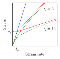
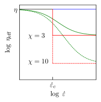
Figure 1: A qualitative comparison of various rheologies. (left) The stress invariant versus strain invariant for isoviscous (blue), simplified pseudoplastic (red), and Cross fluids (green). All fluids have the same small strain rate viscosity. The simplified pseduoplastic and Cross fluids approach the same asymptotic large strain rate viscosity. The parameter $\chi$ is the ratio of small strain rate to large strain rate viscosities, $\chi=\eta/\mu$. Solid and dashed curves correspond to $\xi$ = 3 and 10, respectively. (right) Effective viscosities of the rheological models.

3.2 Planar geometry

In this section, the governing equations are non-dimensionalized and expanded, to leading order, in the thin layer limit for the rheological model described above. This constitutive relation admits determination of the radial velocity profile and radial volume flux. Vertical integration of the continuity equation yields the layer height evolution equation. For cylindrical coordinates ($r$, $z$, $\phi$), the axisymmetric velocity

$$\boldsymbol{u}=u(r,z,t)\,\hat{\mathbf{r}}+w(r,z,t)\,\hat{\mathbf{z}}\;.$$ (3.8)

The vertical locations of the flow base and free surface are $z=0$ and $z=h(r,t)$, respectively. The gravitational acceleration $\boldsymbol{g}=-\,g\hat{\boldsymbol{z}}$.

3.2.1 Non-dimensionalization

Motivated by heuristic arguments (Sec. 2), the governing equations are non-dimensionalized and expanded in the small layer aspect ratio limit. For a rigorous formulation of the expansion in planar axisymmertry the reader is referred to Balmforth et al. [2000]. As in Section 2, let $H$ be the characteristic layer thickness and $L$ be the radial length scale. The vertical coordinate $z$ and layer thickness $h$ are scaled by $H$ while pressure is scaled by $\rho gH$. The radial coordinate $r$ is scaled by $L$. Continuity implies that the vertical velocity scale is first order small with respect to radial velocity. To leading order, the radial velocity scale $V=\rho gH^{3}/\eta L$ representing a balance between lateral pressure gradient and vertical shear stress gradient. Time is scaled by $L/V$. In the thin layer limit, the aspect ratio $H/L$ is the small parameter in which the governing equations are expanded.

3.2.2 Pseudoplastic transition height

To leading order, normal stress is negligible and gravitational body force is balanced by hydrostatic pressure subject to the free surface boundary condition, $\left.p\right|_{z=h}=0$,

$$p=h\,\left(1-\frac{z}{h}\right)\;.$$ (3.9)

The radial pressure gradient due to layer height variation is balanced by vertical shear of the radial flow

$$\frac{\partial p}{\partial r}=\frac{\partial\tau_{rz}}{\partial z}\;.$$ (3.10)

Substituting for $p$, integrating, and applying the boundary condition $\left.\tau_{rz}\right|_{z=h}=0$ yields

$$\tau_{rz}=-hh^{\prime}\,\left(1-\frac{z}{h}\right)\;,$$ (3.11)

where $h^{\prime}=\dfrac{\partial h}{\partial r}$. The stress invariant $\tau=h|h^{\prime}|\,\left(1-\dfrac{z}{h}\right)$ increases as $z$ decreases from $z=h$ and there is a vertical level $Y$ where $\tau=\tau_{c}$,

$$Y=h\left[1-\frac{\tau_{c}}{h|h^{\prime}|}\right]=h\left[1-\frac{2\,\dot{\varepsilon}_{c}}{h|h^{\prime}|}\right]\;.$$ (3.12)

3.2.3 Radial velocity

The constitutive equation implies

$$\tau_{rz}=2\,\eta_{\rm eff}(\dot{\varepsilon})\,\dot{\varepsilon}_{rz}=\eta_{\rm eff}\,(\dot{\varepsilon})\dfrac{\partial u}{\partial z}\;,$$ (3.13)

where the strain rate invariant $\dot{\varepsilon}=\dfrac{1}{2}\,\left|\dfrac{\partial u}{\partial z}\right|$. Let $u_{-}(z)$ be the radial velocity for $z<Y$. Substituting for $\eta_{\rm eff}$, with radial velocity increasing monotically with height $\left(\dfrac{\partial u_{-}}{\partial z}>0\right)$ yields

$$\frac{\partial u_{-}}{\partial z}=-\chi hh^{\prime}\left(1-\frac{z}{h}\right)-2\,(\chi-1)\,\dot{\varepsilon}_{c}\;,$$ (3.14)

where $\chi=\dfrac{\eta}{\mu}$ is the low strain rate to high strain rate viscosity ratio. Integrating with respect to $z$, and applying the no slip boundary condition $\left.u_{-}\right|_{z=0}=0$,

$$u_{-}(z)=-\chi h^{2}h^{\prime}f\left(\frac{z}{h}\right)-2\,(\chi-1)\,h\,\dot{\varepsilon}_{c}\frac{z}{h}\;,\qquad 0\leq z\leq Y\;,$$ (3.15)

with $f(x)=x-x^{2}/2$.

Above $z=Y$, $\eta_{\rm eff}=\eta$, and the momentum balance reduces to the isoviscous case. Letting $u_{+}(z)$ be the velocity for $z>Y$,

$$\frac{\partial u_{+}}{\partial z}=-hh^{\prime}\left(1-\frac{z}{h}\right)\;.$$ (3.16)

Integrating and matching velocities $u_{-}(Y)=u_{+}(Y)$ gives,

$$u_{+}(z)=-h^{2}h^{\prime}f\left(\frac{z}{h}\right)-(\chi-1)\,h^{2}h^{\prime}f\left(\frac{Y}{h}\right)-2\,(\chi-1)\,h\,\dot{\varepsilon}_{c}\frac{Y}{h}\;,\qquad Y\leq z\leq h\;.$$ (3.17)

Eliminating the transition strain rate using Eq. (3.12),

$$u(z)=\begin{cases}-h^{2}h^{\prime}\left[\chi f\left(\dfrac{z}{h}\right)-(\chi-1)\left(1-\dfrac{Y}{h}\right)\dfrac{z}{h}\right]&0\leq z\leq Y\\[10.00002pt] -h^{2}h^{\prime}\left[f\left(\dfrac{z}{h}\right)+(\chi-1)\dfrac{Y^{2}}{2h^{2}}\right]&Y\leq z\leq h\end{cases}$$ (3.18)

This velocity distribution is shown in Fig. 2. In the limit $Y\rightarrow 0$, the velocity $u(z)=-h^{2}h^{\prime}f(z/h)$ which corresponds to the $\eta_{\rm eff}\rightarrow\eta$ isoviscous limit. Likewise, when $Y\rightarrow h$, $u(z)=-\chi h^{2}h^{\prime}f(z/h)$ which is the $\eta_{\rm eff}\rightarrow\mu$ isoviscous limit.

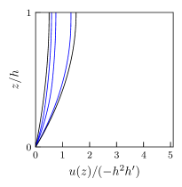
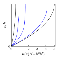
Figure 2: Radial velocity profiles for the cases $\chi=3$ (left), $\chi=10$ (right), and different pseduoplastic transition levels (left to right) $Y/h$ = (0, 0.3, 0.5, 0.9, 1). The black curves correspond to the low strain rate and high strain rate isoviscous limits (see discussion in text).

The height evolution equation (see next section) depends on the vertically integrated radial velocity, i.e., the radial volume flux per unit azimuthal length

$$U=\int_{0}^{Y}u_{-}(z)\,dz+\int_{Y}^{h}u_{+}(z)\,dz\;.$$ (3.19)

Evaluating,

$$U=-h^{3}h^{\prime}\left[\frac{1}{3}+\frac{1}{2}\,(\chi-1)\left(\frac{Y}{h}\right)^{2}\left(1-\frac{Y}{3h}\right)\right]\;.$$ (3.20)

In the low strain rate $Y\rightarrow 0$ limit, $U$ reduces to the isoviscous $\eta_{\rm eff}\rightarrow\eta$ case, i.e., $U=-h^{3}h^{\prime}/3$. Likewise for $Y\rightarrow h$, $U=-\chi h^{3}h^{\prime}/3$ which is the $\eta_{\rm eff}\rightarrow\mu$ isoviscous limit.

3.2.4 Evolution equation

The free surface kinematic condition

$$\frac{\partial h}{\partial t}+u(r,h,t)\frac{\partial h}{\partial r}-w(r,h,t)=0\;.$$ (3.21)

Vertically integrating the continuity equation over the layer height subject to basal and free surface boundary conditions and identifying $w(r,0,t)=w_{s}(r,t)$ yields the layer height evolution equation representing mass conservation,

$$\frac{\partial h}{\partial t}+\frac{1}{r}\frac{\partial}{\partial r}\left(rU\right)=w_{s}(r,t)\;,$$ (3.22)

where $U$ is given by Eq. (3.20).

3.3 Spherical geometry

The following section is a brief outline the thin layer expansion in spherical geometry. It is shown that, to leading order, local flow on a sufficiently large sphere is insensitive to substrate curvature resulting in polar velocity and volume flux identical to the planar case. In spherical coordinates ($\theta$, $r$, $\phi$), the axisymmetric velocity field

$$\boldsymbol{u}=u(\theta,r,t)\,\hat{\boldsymbol{\theta}}+w(\theta,r,t)\,\hat{\boldsymbol{r}}\;.$$ (3.23)

The radial locations of the flow base and free surface are $r=R$ and $r=R+h(\theta,t)$, respectively. The gravitational acceleration $\boldsymbol{g}=-\,g\,\hat{\boldsymbol{r}}$. The layer is considered to extend laterally along an arclength $R\,\theta_{f}(t)$. The thin layer approximation $h\ll R\,\theta_{f}$ is assumed to hold throughout spreading given sufficiently large substrate curvature $R$. Because $\theta_{f}\sim 1$, it follows that $h\ll R$.

The radius of curvature $R$ provides an intrinsic lengthscale for non-dimensionlization. Lengths are scaled by $R$ and pressure by $\rho gR$. The polar velocity scale $V=\rho gR^{2}/\eta$ and timescale is $R/V$. Upon non-dimensionalizing, the quantity in which the governing equations are expanded is $h\ll 1$. A change of variables is introduced

$$r=1+\xi\;,$$ (3.24)

where $0\leq\xi\leq h$ is the non-dimensional radial coordinate measured from the spherical surface.

The radial pressure gradient balances the gravitational body force subject to the free surface boundary condition $\left.p\right|_{\xi=h}=0$,

$$p=h\,\left(1-\frac{\xi}{h}\right)\;.$$ (3.25)

The polar pressure gradient due to layer height variation is balanced by radial shear of the polar flow. In terms of $\xi$,

$$\frac{1}{(1+\xi)}\frac{\partial p}{\partial\theta}=\frac{1}{(1+\xi)^{2}}\frac{\partial}{\partial\xi}\left((1+\xi)^{2}\tau_{\xi\theta}\right))\;.$$ (3.26)

Substituting for $p$, applying the boundary condition $\left.\tau_{\xi\theta}\right|_{\xi=0}=0$, and dropping terms ${\cal{O}}(h^{2})$ and higher,

$$\tau_{\xi\theta}=-hh^{\prime}\left(1-\frac{\xi}{h}\right)\;,$$ (3.27)

where $h^{\prime}=\dfrac{\partial h}{\partial\theta}$. This linear stress distribution is identical to the planar case Eq. (3.11). Thus, the radial level $\xi=Y$ below which the stress invariant exceeds $\tau_{c}$ is given by Eq. (3.12).

To leading order, the constitutive equation

$$\tau_{\xi\theta}=2\,\eta_{\rm eff}(\dot{\varepsilon})\,\dot{\varepsilon}_{\xi\theta}=\eta_{\rm eff}\,(\dot{\varepsilon})\dfrac{\partial u}{\partial\theta}\;,$$ (3.28)

where the strain rate invariant $\dot{\varepsilon}=\dfrac{1}{2}\,\left|\dfrac{\partial u}{\partial\theta}\right|$. Analysis proceeds as in the planar case. The polar velocities $u_{\pm}(\xi)$ above and below $Y$ satisfy Eqs. (3.16) and (3.14), respectively. The polar velocity profile $u(\xi)$ and polar volume flux per unit azimuthal length $U$ are given by Eqs. (3.18) and (3.20), respectively, with $h^{\prime}\rightarrow\dfrac{\partial h}{\partial\theta}$ and $z\rightarrow\xi$.

To leading order, in terms of $(\theta,\xi,t)$, the free surface kinematic condition,

$$\frac{\partial h}{\partial t}+u(\theta,h,t)\frac{\partial h}{\partial\theta}-w(\theta,h,t)=0\;.$$ (3.29)

Radially integrating the continuity equation subject to basal and free surface boundary conditions, identifying $w(\theta,0,t)=w_{s}(\theta,t)$ and dropping terms $\mathcal{O}(h^{2})$ and higher yields

$$\frac{\partial h}{\partial t}+\left[\frac{1}{\sin\theta}\frac{\partial}{\partial\theta}\left(\sin\theta\,U\right)\right]=w_{s}(\theta,t)\;,$$ (3.30)

where $U$ is given by Eq. (3.20)

4 Numerical results

4.1 Planar geometry

Variation of rheological transition stress and viscosity ratio are investigated numerically. The transition stress range is chosen to include anticipated end-member behaviors. The non-dimensional source function

$$w_{s}(r)=w_{0}\,(r_{0}^{2}-r^{2})\,H(r_{0}-r)\;,$$ (4.1)

where $r_{0}$ = 0.15, $w_{0}$ = 0.1, and $H$ is the unit step function.

4.1.1 Height field

The effect of varying the pseudoplastic transition stress is considered for viscosity ratio $\chi$ = 10. For large transition stress ($\tau_{c}=300\times 10^{-4}$), the location of the rheological transition surface $Y$ is indistinguishable from zero except for small regions near the flow front (Fig. 3). Also, the solution converges to the similarity solution in the similarity variable $\zeta=r/t^{1/2}$. away from the source. Thus, the fluid behaves isoviscously with $\eta_{\rm eff}\approx\eta$.

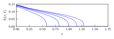
Figure 3: Evolution for $\tau_{c}=300\times 10^{-4}$ and $\chi=10$. (top) Layer height field $h(r,t)$ (blue) together with the transition surface $Y(r,t)$ (red, dashed) for non-dimensional times (1, 2, 3, 4, 5) $\times$ 10³. The transition surface location $Y=0$ except for small regions around the flow front. (bottom) Layer height field versus the similarity variable $\zeta=r/t^{1/2}$. Away from the source, solution convergence onto the similarity form indicates that the fluid behaves isoviscously with $\eta_{\rm eff}\approx\eta$.

For intermediate transition stress ($\tau_{c}=30\times 10^{-4}$), the location of the transition surface is initially approximately half of the layer height but decreases as evolution proceeds (Fig. 4). In this case, it is not possible to collapse the solution onto a similarity form.

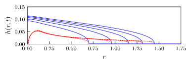
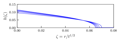
Figure 4: As Fig. 3 with $\tau_{c}=30\times 10^{-4}$. (top) Height field and pseudoplastic transition surface located at approximately half the layer height. (bottom) Height field as a function of the similarity variable $\zeta$. For intermediate transition stress, a similarity solution of the isoviscous form is not admitted.

For small transition stress ($\tau_{c}=3\times 10^{-4}$), the transition surface location is approximately equal to layer height (Fig. 5). Scaling layer height and radius by the appropriate viscosity ratio factors (Sec. 2) indicates that the solution is converging to an isoviscous similarity solution with high strain rate viscosity $\eta_{\rm eff}\approx\mu$.

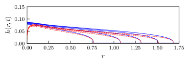
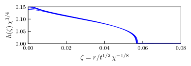
Figure 5: As Fig. 3 with $\tau_{c}=3\times 10^{-4}$. (top) Height field and pseudoplastic transition surface with location approximately equal to the layer height. (bottom) Height field scaled by the viscosity ratio factor $\chi^{1/4}$ as a function of the similarity variable $\zeta$ scaled by the viscosity ratio factor $\chi^{-1/8}$. The approximate convergence of the solution onto the similarity form suggests the flow is effectively isoviscous with $\eta_{\rm eff}\rightarrow\mu$.

4.1.2 Flow front

In Fig. 6, flow front location as a function of time is shown for viscosity ratio $\chi$ = 10 and three values of transition stress. The flow front is defined by $h(r_{f},t)$ = 0.01. For sufficiently large $\tau_{c}$, flow is controlled by the low strain rate viscosity, i.e., $\eta_{\rm eff}\approx\eta$ and flow radius exhibits the asymptotic, isoviscous, time scaling. Also, for small transition stress, the flow behaves isoviscously with $\eta_{\rm eff}\approx\mu$ throughout the evolution time considered. In the case of intermediate $\tau_{c}$, flow radius behavior exhibits a transition. Initially, layer evolution is consistent with the $\eta_{\rm eff}\approx\mu$ regime. As the layer spreads, the stress invariant decreases, and the behavior approaches that for the small strain rate limit.

Scaling analysis (Sec. 2) suggests that, for spreading initially controlled by $\mu$, shear stress decreases with time like $t^{-1/2}$. That is, the dimensional stress invariant,

$$\tau\sim\left(\rho^{3}g^{3}\mu^{5}Q\right)^{1/8}\;t^{-1/2}\;.$$ (4.2)

A flow transition time scale $t_{c}$ can be defined as the time when $\tau\sim\tau_{c}$

$$t_{c}\sim\frac{\left(\rho^{3}g^{3}\mu^{5}Q\right)^{1/4}}{\tau_{c}^{2}}\;.$$ (4.3)

Non-dimensionalizing (Sec. 3.2.1),

$$t_{c}\sim\frac{Q^{1/4}}{\chi^{5/4}\tau_{c}^{2}}\;.$$ (4.4)

For non-dimensional source function Eq. (4.1), $Q=\dfrac{\pi}{2}w_{0}r_{0}^{4}$

$$t_{c}\sim 10^{3}\,\left(\frac{10}{\chi}\right)^{5/4}\,\left(\frac{30\times 10^{-4}}{\tau_{c}}\right)^{2}\;.$$ (4.5)

Thus, the intermediate transition stress case is expected to undergo this flow transition during the non-dimensional evolution time of the calculation $T=5\times 10^{3}$. The low transition stress case considered would not exhibit such behavior until a non-dimensional time $t\sim 10^{2}\,T$.

For fixed transition stress and evolution time, increasing viscosity ratio $\chi$ implies increasing flow radius (Eq. 2.7). For $\tau_{c}=3\times 10^{-4}$ and $T=5\times 10^{3}$, flow radius was calculated as a function of $\chi$. Results agree with the scaling analysis (Fig. 6).

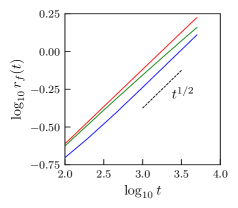
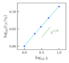
Figure 6: (left) Variation in flow front radius with time for $\chi$=10 and pseudoplastic transition stress $\tau_{c}=(300,30,3)\times 10^{-4}$ (blue, greed, red). The black dashed line shows the characteristic, isoviscous scaling. (right) Flow front location after fixed evolution time $T=5\times 10^{3}$ for $\tau_{c}=3\times 10^{-4}$ as a function of viscosity ratio $\chi$. Results are in good agreement with the expected asympotic scaling (green dashed line).

4.2 Spherical geometry

In spherical geometry, the non-dimensional source function

$$w_{s}(\theta)=w_{0}\,(\theta_{0}^{2}-\theta^{2})\,H(\theta_{0}-\theta)$$ (4.6)

with $\theta_{0}$ = 0.15 and $w_{0}$ = 0.1. This source corresponds to non-dimensional volume flux $Q$ identical to the planar geometry volume flux to $\mathcal{O}(\theta_{0}^{5})$. In the following sections, the effects of varying rheological transition stress and viscosity ratio are investigated numerically.

4.2.1 Height field

The range of rheological transition stresses investigated in spherical geometry is the same as that for the planar geometry case. Likewise, the viscosity ratio $\chi$ = 10. Results are summarized in Fig. (7). For large transition stress ($\tau_{c}=300\times 10^{-4}$), the location of the rheological transition surface $Y\sim 0$. In this limit, the fluid behaves isoviscously with $\eta_{\rm eff}\approx\eta$. For intermediate transition stress ($\tau_{c}=30\times 10^{-4}$), the low viscosity part of the flow is initially approximately half of the layer height. The low viscosity layer height fraction decreases as evolution proceeds. For small transition stress ($\tau_{c}=3\times 10^{-4}$), $Y\sim h$.

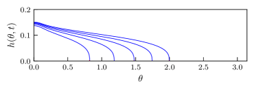
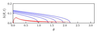
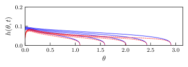
Figure 7: Evolution in spherical geometry for $\chi=10$ and, from top to bottom, $\tau_{c}=(300,30,3)\times 10^{-4}$, respectively. Layer height fields $h(\theta,t)$ (blue) together with the transition surface $Y(\theta,t)$ (red, dashed) for non-dimensional times (2, 4, 6, 8, 10) $\times$ 10³. (top) The transition surface location is indistinguishable from $Y=0$. (middle) The low viscosity region constitutes a decreasing fraction of the layer height throughout evolution. (bottom) The high viscosity part of the flow is only a small fraction near the free surface.

4.2.2 Flow front

The flow front location is defined by $h(\theta_{f},t)$ = 0.01. As in the planar case, the flow front location is controlled by high (low) viscosities for large (small) rheological transition stress (Fig. LABEL:eq:sphr_front). In the intermediate $\tau_{c}$ case, flow dynamics transition during evolution due to decreasing low viscosity layer fraction. In spherical geometry, isolation of the viscosity ratio effect is complicated by transition to a converging flow front when spreading proceeds past the equatorial polar angle. To isolate rheological influence on layer dynamics, the time for spreading to $\theta_{f}\sim\pi/2$ is calculated as a function of viscosity ratio $\chi$. Scaling analysis (Sec. 2) suggests that the time for spreading to polar angle $\theta_{f}$ for $\eta_{\rm eff}\sim\eta$,

$$t^{\ast}\sim\left(\frac{Q^{3}\rho g}{\eta}\right)\theta_{f}^{2}\;.$$ (4.7)

In the asymptotic limit, $\eta_{\rm eff}\sim\mu$,

$$t_{\mu}^{\ast}\sim\chi^{-1/4}\;t^{\ast}\;.$$ (4.8)

Numerical results (Fig. 8) are in good agreement with the anticipated scaling.

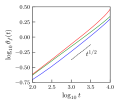
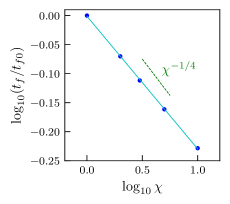
Figure 8: (left) Variation in flow front polar angle with time for $\chi$=10 and pseudoplastic transition stress $\tau_{c}=(300,30,3)\times 10^{-4}$ (blue, greed, red). The black dashed line shows the characteristic, isoviscous scaling. (right) Time for spreading to equatorial polar angle as a function of viscosity ratio $\chi$. Flow behavior is in agreement with asymptotic scaling analysis (green dashed line).

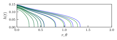
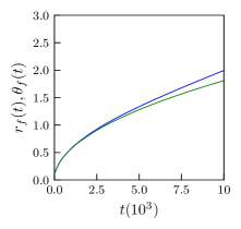
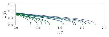
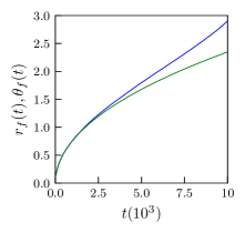
Figure 9: (top,left) Height fields $h(\theta,t)$ and $h(r,t)$ in spherical (blue) and planar (green) geometries for the isoviscous (or large transition stress) and non-dimensional times (0.2, 0.4, 0.6, 0.8, 1, 2, 3, 4, 5) $\times$ 10³. (top,right) Flow front location as a function of time. For polar angle $\theta\lesssim 0.5$, the solutions are in good agreement. (bottom) As for the top figures for the case $\tau_{c}=3\times 10^{-4}$ and $\chi$ = 10.

4.3 Small polar angle approximation

In the small polar angle limit $\theta\ll 1$, the non-dimensional evolution equation for layer height in spherical geometry reduces to that for planar geometry. Planar and spherical solutions for identical source functions should be equal in the small polar angle approximation. Layer height fields and flow front location for the two geometries are compared in Fig. (9) for the isoviscous and small transition stress cases. Solutions are in agreement for polar angle $\theta\lesssim 0.5$. For example, the relative difference in flow front location at this angle is $\sim$ 0.3 %

5 Conclusions

A pseudoplastic rheology was applied to axisymmetric thin film evolution in planar and spherical geometries with constant volume flux source. Closed form expressions for velocity profile and volume flux were derived. The numerical approach utilized in the study was benchmarked against previous analytical and numerical solutions. Influence of rheological transition strain rate and viscosity ratio on layer evolution was explored numerically. In the limits of large and small transition strain rate, approximately isoviscous evolution was observed. For intermediate transition strain rate, control of layer spreading can undergo an adjustment from high to low strain rate viscosity. Planar and spherical geometry solutions agree for sufficiently small polar angle (see e.g., Takagi and Huppert [2010]).

While admittedly simplified, the rheological model captures bulk features of shear thinning and allows for efficient exploration of parameter space. It may find applicability in geodynamical contexts including, but not limited to, plume head evolution Bercovici and Lin [1996], isostatic adjustment to thermochemical diapirs [Watters et al., 2009], and glacial dynamics [Schoof et al., 2010]. The rheology is also adaptable to channelized flow [Sochi, 2015] and, as silicic magmas exhibit shear thinning behavior [Jones et al.,, 2020; Vasseur et al., 2023], could be implemented in models of dike emplacement and/or magma flow in volcanic conduits [Gonnermann and Manga, 2007]. The pseudoplastic model is readily extendable to spreading on substrates with constant radius of curvature and vertical gravitational acceleration [Takagi and Huppert, 2010] relevant to industrial coating applications. Finally, modification of the model to more complex, non-planar surfaces [Lin et al., 2012, 2021] is also a possibility.

6 Appendix: Numerical method

In this appendix, the numerical method is benchmarked against analytical solutions and other numerical approaches. Layer height evolution equations (Eqs. 3.22,3.30) are of the form

$$\frac{\partial h(r,t)}{\partial t}=\mathcal{D}\left[h(r,t)\right]$$ (6.1)

where $\mathcal{D}$ is a non-linear differential operator. The Python package py-pde [Zwicker, 2020] provides methods for solving partial differential equations of this form. The py-pde, method-of-lines scheme utilizes implicit, Adams backward differentiation [Hindmarsh, 1983; Petzold, 1983]. To benchmark the numerical approaches, the isoviscous, constant volume flux source case is considered and compared to analytical and numerical solutions.

6.1 Planar geometry

The source function used for pseudoplasticity (Eq. 4.1) is adopted for the isoviscous benchmark. Likewise, the initial and boundary conditions for $h(r,t)$ are the same as those for the pseudoplastic rheology. In the limit of a constant, point source flux $w_{s}$, the isoviscous case admits an analytical, similarity solution [Huppert, 1982a] in the similarity variable $\zeta=r/t^{1/2}$. Sufficiently far from the source, numerical solutions converge to the similarity form (Fig. 10). The flow front location scales with $t^{1/2}$ as expected from the similarity solution and asymptotic scaling analysis [Griffiths and Fink, 1993].

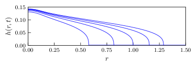
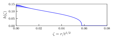
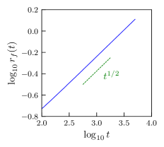
Figure 10: (left,top) Isoviscous height field evolution in planar geometry. Snapshots of the flow height profile every 10³ non-dimensional times units are shown. (left,bottom) Height field evolution scaled by $t^{1/2}$ as a function of the similarity variable $\zeta=r/t^{1/2}$. Away from the source, solutions converge to the similarity form. (right) Flow front location $r_{f}$ defined as the non-dimensional height where $h(r_{f},t)=0.01$. After initial transient behavior [Ball and Huppert, 2019], numerical results agree with the expected asymptotic scaling.

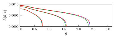
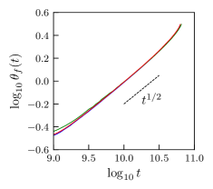
Figure 11: Comparison of the numerical method for spherical geometry with previous results. (left) Isoviscous height field evolution. Results are shown for a case with $\theta_{w}=0.3$ and non-dimensional source amplitude $w_{0}^{\prime}=7.9\times 10^{-13}$. Snapshots of the flow height profile for non-dimensional times (0.614, 2.46, 4.77) $\times$ 10¹⁰. (green) yin-yang grid, (red) adaptive grid, (blue) Python py-pde. (right) Flow front location $\theta_{f}(t)$ defined as the angular location where non-dimensional height $h(r_{f},t)=0.01\;h(0,t)$. Results are in good agreement throughout spreading. Line colors correspond to the top figure.

6.2 Spherical geometry

In the absence of a similarity solution in spherical geometry, the numerical method adopted in this work is benchmarked against previous numerical results [Reese et al., 2010, 2011]. One previous approach uses an adaptive grid scheme designed for nonlinear parabolic equations [Blom and Zegeling, 1994] adopted for axisymmetric spreading on a spherical surface. Another method utilizes a composite, overlapping [Chesshire and Henshaw, 1990] “yin-yang” grid [Kageyama and Sato, 2004; Kageyama, 2005]. This method decomposes the sphere into two component grids, one being a low to mid-latitude portion of a standard spherical-polar grid and the other a rotation of the first and is explicitly two-dimensional in ($\theta$, $\phi$). That is, in the axisymmetric, isoviscous case (or small strain rate limit for pseudoplastic rheology), the layer height evolution equation Eq. (3.30) reduces to

$$\frac{\partial h}{\partial t}=\frac{1}{12}\nabla^{2}_{\theta}h^{4}+w_{s}(\theta,t)\;,$$ (6.2)

where $\nabla_{\theta}$ is the polar angle part of the Laplacian on the unit sphere. The “yin-yang” grid method integrates the evolution equation for flow thickness in time using an explicit Euler scheme and standard, centered, second-order approximations for the full tangential Laplacian operator $\nabla^{2}_{\theta}+\nabla^{2}_{\phi}$. The solution at the component grid boundaries are determined by bilinear interpolation from neighboring points. Source axisymmetry results in axisymmetric layer spreading.

To accommodate the benchmark, the constant volume flux source function is modified to that used in Reese et al. [2010]. In that study, the source function is a truncated gaussian,

$$w_{s}(\theta)=w_{0}\;\exp(-\theta^{2}/\theta_{w}^{2})\;H(\theta_{0}-\theta)\;.$$

As for the pseudoplastic cases, the initial condition $h(\theta,t=0)$ is a small, finite, smoothly varying function. The gradient of $h$ at the edges of the domain is set to zero.

Good agreement between methods is found for both flow front location as a function of time and flow profile as a function of $\theta$. Also shown is the characteristic scaling (dashed line) for the planar geometry, constant volume flux case [Huppert, 1982a]. The flow front eventually converges on the source antipode, $\log\theta_{f}\approx$ 0.5. For sufficiently small distance from the anitpodal axis of symmetry, a regime transition occurs [Gratton and Minotti, 1990; Diez et al., 1992] which appears to be resolved in the solutions (Fig. 11).

References

- Algwauish [2019] Algwauish, G.M.S.A. (2019), The non-Newtonian and non-isothermal spreading of liquid domes using mathematical and numerical methods, Doctoral dissertation, Keele University.
- Ancey [2007] Ancey, C. (2007), Plasticity and geophysical flows: A review, JṄon-Newton. Fluid Mech., 142, 4-35.
- Ball and Huppert [2019] Ball, T.V. and Huppert, H.E. (2019), Similarity solutions and viscous gravity current adjustment times, J. Fluid Mech., 874, 285-298.
- Balmforth and Craster [1999] Balmforth, N.J. and Craster, R.V. (1999), A consistent thin-layer theory for Bingham plastics, J. Non-Newton. Fluid Mech., 84, 65-81.
- Balmforth et al. [2000] Balmforth, N.J., Burbridge, A.S., Craster, R.V., Salzig, J. and Shen, A. (2000), Visco-plastic models of isothermal lava domes, J. Fluid Mech., 403, 37-65.
- Balmforth et al. [2004] Balmforth, N.J., Craster, R.V., and Sassi, R. (2004), Dynamics of cooling viscoplastic domes, J. Fluid Mech., 499, 149-182.
- Balmforth et al. [2006] Balmforth, N.J., Craster, R.V., Rust, A.C. and Sassi, R. (2006), Viscoplastic flow over an inclined surface, J. Non-Newton. Fluid Mech., 139, 103-127.
- Bercovici [1994] Bercovici, D. (1994), A theoretical model of cooling viscous gravity currents with temperature-dependent viscosity, Geophys. Res. Lett., 21, 1177-1180.
- Bercovici and Lin [1996] Bercovici, D. and Lin, J. (1996), A gravity current model of cooling mantle plume heads with temperature dependent buoyancy and viscosity, J. Geophys. Res., 101, 3291-3309.
- Bird et al. [1987] Bird, R., Armstrong, R., and Hassager, O. (1987), Dynamics of Polymeric Liquids. Wiley.
- Blake [1990] Blake, S. (1990), Viscoplastic models of lava domes, Lava Flows and Domes: Emplacement Mechanisms and Hazard Implications (ed. J.H. Fink), IAVCEI Proceedings in Volcanology, 2, 88-128.
- Blom and Zegeling [1994] Blom, J.G., and Zegeling, P.A. (1994), Algorithm 731: A moving grid interface for systems of one dimensional time dependent partial differential equations, ACM Trans. Math. Software, 20, 194-214.
- Chesshire and Henshaw [1990] Chesshire, G., and Henshaw, W. (1990), Composite overlapping meshes for the solution of partial differential equations, J. Comp. Phys., 90, 1-64.
- Diez et al. [1992] Diez, J.A., Gratton, G., and Gratton, J. (1992), Self-similar solution of the second kind for a convergent viscous gravity current, Phys. Fluids A, 4, 1148-1155.
- Gonnermann and Manga [2007] Gonnermann, H.M. and Manga, M. (2007), The fluid mechanics inside a volcano, Ann. Rev. Fluid Mech., 39, 321-356.
- Gratton and Minotti [1990] Gratton, J., and Minotti, F. (1990), Self-similar viscous gravity currents: Phase plane formalism, J. Fluid Mech., 210, 155-182.
- Gratton et al. [1999] Gratton, J., Minotti, F., and Mahajan, S.M. (1999), Theory of creeping gravity currents of a non-Newtonian liquid, Phys. Rev. E, 60, 6960-6967.
- Griffiths and Fink [1993] Griffiths, R.W. and Fink J.H. (1993), Effects of surface cooling on the spreading of lava flows and domes, J. Fluid Mech., 252, 667-702.
- Hindmarsh [1983] Hindmarsh, A.C. (1983), ODEPACK, A systemized collection of ODE solvers, Scientific Computing (ed. R.S. Stepleman et al.), IMACS Trans. Sci. Comp. 1, 55-64.
- Huppert [1982a] Huppert, H.E. (1982a), The propagation of two-dimensional and axisymmetric viscous gravity currents over a rigid horizontal surface, J. Fluid Mech., 121, 43-58.
- Huppert [1982b] Huppert, H.E. (1982b), Flow and instability of a viscous current down a slope, Nature, 300, 427-229.
- Huppert [2006] Huppert, H.E. (2006), Gravity currents: a personal perspective, J. Fluid Mech., 554, 299-322.
- James et al. [2021] James, F., M’ Baye, M., Msheik, K. and Nguyen, D. (2021), A lubrication equation for a simplified model of shear thinning fluid, ESAIM: Proceedings and Surveys, 70, pp.147-165.
- Jones et al., [2020] Jones, T.J., Llewellini, E.W., and Mader, H.M., (2020), The use of a shear-thinning polymer as a bubbly magma analogue for scaled laboratory experiments, J. Volcanol. Geotherm. Res., 392, 106768.
- Kageyama and Sato [2004] Kageyama, A. and Sato, T. (2004), “Yin-Yang grid”: An overset grid in spherical geometry, Geochem. Geophys. Geosyst., 5, Q09005.
- Kageyama [2005] Kageyama, A. (2005), Dissection of a sphere and yin-yang grids, J. of the Earth Sim., 3, 20-28.
- Kang et al. [2016] Kang, D., Nadim, A., and Chugnova, M. (2016), Dynamics and equilibria of thin viscous coating films on a rotating sphere, J. Fluid Mech., 791, 495-518.
- Kang et al. [2017] Kang, D., Nadim, A., and Chugnova, M. (2017), Marangoni effects on a thin liquid film coating a sphere with axial or radial thermal gradients, Phys. Fluids, 29, 1-15.
- Kerr and Mériaux [2004] Kerr, R.C. and Mériaux, C. (2004), Structure and dynamics of sheared mantle plumes, Geochem. Geophys. Geosyst., 5, Q12009.
- Lavallée et al. [2007] Lavallée, Y., Hess, K.U., Cordonnier, B., and Dingwill, D.B. (2007), Non-Newtonian rheological law for highly crystalline dome lavas, Geology, 35, 843-846.
- Lin et al. [2012] Lin, T-S, Kondic, L., and Filipov, A. (2012), Thin films flowing down inverted substrates: Three dimensional flow, Phys. Fluids, 24, 022105.
- Lin et al. [2021] LIn, T-S, Dijksman, J.A., and Kondic, L. (2021), Thin liquid films in a funnel, J. Fluid Mech., 924, A26.
- Myers [2005] Myers, T.G., (2005), Application of non-Newtonian models to thin film flow, Phys. Rev. E, 72, 066302.
- Neossi Nguetchue and Momoniat [2007] Neossi Nguetchue, S.N. and Momoniat, E. (2007), Axisymmetric spreading of a thin power law fluid under gravity on a horizontal plane, Nonlinear Dyn., 52, 361-366.
- Oron et al. [1997] Oron, A., Davis, S.H., and Bankoff, G. (1997), Long-scale evolution of thin liquid films, Rev. Modern Phys., 69, 931-980.
- Perazzo and Gratton [2003] Perazzo, C.A. and Gratton, J. (2003), Thin film of non-Newtonian fluid on an incline, Phys. Rev. E, 67, 016307.
- Petzold [1983] Petzold, L. (1983), Automatic selection of methods for solving stiff and nonstiff systems of ordinary differential equations, SIAM J. Sci. Stat. Comput., 4, 136-148.
- Pritchard et al. [2015] Pritchard, D., Duffy, B.R., and Wilson, S.K. (2015), Shallow flows of generalised Newtonian fluids on an inclined plane, J. Eng. Math., 94, 115-133.
- Reese et al. [2010] Reese, C.C., Orth, C.P., and Solomatov, V.S. (2010), Impact origin for the Martian crustal dichotomy: Half emptied or half filled?, J. Geophys. Res., 115.
- Reese et al. [2011] Reese, C.C., Orth, C.P., and Solomatov, V.S. (2011), Impact megadomes and the origin of the martian crustal dichotomy, Icarus, 213, 433-442.
- Roy et al. [2002] Roy, R.V., Roberts, A.J., and Simpson, M.E. (2002), A lubrication model of coating flows over a curved substrate in space, J. Fluid Mech., 454, 235-261.
- Schoof et al. [2010] Schoof, C., and Hindmarsh, C.A. (2010), Thin-film flows with wall slip: An asymptotic analysis of higher order glacier flow models, Q. J. Mech. Appl. Math., 63, 73-114.
- Simpson [1999] Simpson, J.E. (1999), Gravity Currents: In the Environment and the Laboratory, 2nd ed. Cambridge University Press.
- Sochi [2015] Sochi, T. (2015), Analytical solutions for the flow of Carreau and Cross fluids in circular pipes and thin slits, Rheol. Acta, 54, 745-756.
- Stasuik et al. [1993] Stasuik, M.V., Jaupart, C., and Sparks, R.S.J. (1993), Influence of cooling on lava flow dynamics, Geology, 21, 335-338.
- Takagi and Huppert [2010] Takagi, D. and Huppert, H.E. (2010), Flow and instability of thin films on a cylinder and sphere, J. Fluid Mech., 647, 221-238.
- Taranets [2019] Taranets, R.M. (2019), Thin-film flows on a solid sphere, J. Math. Sci, 243, 493-504.
- Ungarish [2009] Ungarish, M. (2009), An introduction to Gravity Currents and Intrusions. CRC Press.
- Vasseur et al. [2023] Vasseur, J., Wadsworth, F.B., and Dingwell, D.B. (2023), Shear thinning and brittle failure in crystal-bearing magmas arise from local non-Newtonian effects in the melt, Earth Planet. Sci., 603, 117988.
- Watters et al. [2009] Watters, W.A., Zuber, M.T., and Hager, B.H. (2009), Thermal perturbations caused by large impacts and consequences for mantle convection, J. Geophys. Res., 114, E02001.
- Wrobel [2020] Wrobel, M. (2020), An efficient algorithm of solution for the flow of generalized Newtonian fluid in channels of simple geometries, Rheol. Acta, 59, 651-663.
- Zwicker [2020] Zwicker, D. (2020), py-pde: A Python package for solving partial differential equations, J. Open Source Softw., 5(48), 2158.