The competent Computational Thinking test (cCTt): a valid, reliable and gender-fair test for longitudinal CT studies in grades 3-6

Abstract

The introduction of computing education into curricula worldwide requires multi-year assessments to evaluate the long-term impact on learning. However, no single Computational Thinking (CT) assessment spans primary school, and no group of CT assessments provides a means of transitioning between instruments. This study therefore investigated whether the competent CT test (cCTt) could evaluate learning reliably from grades 3 to 6 (ages 7-11) using data from 2709 students. The psychometric analysis employed Classical Test Theory, normalised z-scoring, Item Response Theory, including Differential Item Functioning and PISA’s methodology to establish proficiency levels. The findings indicate that the cCTt is valid, reliable and gender-fair for grades 3-6, although more complex items would be beneficial for grades 5-6. Grade-specific proficiency levels are provided to help tailor interventions, with a normalised scoring system to compare students across and between grades, and help establish transitions between instruments. To improve the utility of CT assessments among researchers, educators and practitioners, the findings emphasise the importance of i) developing and validating gender-fair, grade-specific, instruments aligned with students’ cognitive maturation, and providing ii) proficiency levels, and iii) equivalency scales to transition between assessments. To conclude, the study provides insight into the design of longitudinal developmentally appropriate assessments and interventions.

1 Introduction and related work

1.1 The relevance of research on Computational Thinking assessments

Research around Computational Thinking has been increasing significantly over the past two decades with studies touching “different countries, subjects, research issues, and teaching tools hav[ing] also become more diverse in recent years” (Hsu et al., 2018). While there is no universally accepted definition of CT, Brennan and Resnick (2012)’s operational definition helps decompose CT into three dimensions: i) the concepts that designers engage with as they program, ii) the practices that they develop as they engage with these concepts, and finally iii) the perspectives that they form regarding the world and themselves. Many researchers have advocated that CT is a competence that is not specific to CS, that all should acquire (Wing, 2006), and that has potential for learning and meta-cognition (Yadav et al., 2022), with recent studies having demonstrated the link between CT and other abilities (Xu et al., 2021, 2022; Li et al., 2021; Tsarava et al., 2022). Therefore, it is not surprising to see an increasing number of countries looking to or presently introducing Computational Thinking (or the closely related Computer Science, or even more broadly Digital Education) in their curricula throughout K-12 (Weintrop et al., 2021; Commission et al., 2022). However, to be able to teach CT, guide students and provide feedback from the teachers’ perspective (Hsu et al., 2018), or design and validate CT-interventions from the researchers’ perspective, it is essential to have reliable and validated CT assessments spanning K-12 (Commission et al., 2022). Unfortunately, the use of validated CT assessments is something that Tang et al. (2020) noted was lacking in approximately 50% of CT-related studies. From the practitioners’ perspective, assessment issues need to be resolved for successful integration of CT in K-12 curricula (Cutumisu et al., 2019). This is because the “purpose of an assessment is to facilitate student learning” (Guggemos et al., 2022) and “validated assessments […] measure students’ progress in meeting the learning outcomes prescribed by the programs of study” (Cutumisu et al., 2019). It thus becomes paramount to develop and guide “researchers and practitioners in choosing developmentally appropriate CT assessments” (Cutumisu et al., 2019). It is therefore not surprising to see that CT assessment “is at the forefront of CT research [and] gathering the greatest interest of researchers” (Tikva and Tambouris, 2021).

1.2 The lack of validated and reliable assessments at all levels of schooling, namely primary school

According to Tang et al. (2020)’s meta review, CT assessments are provided in four formats. The first are portfolios, which are the most common assessment format, but are likely to conflate with programming abilities, cannot be used in pre-post assessments and are difficult to scale up, in addition to being difficult to standardise and thus provide evidence of validity and reliability. The second are interviews, which suffer from the same limitations as Portfolio assessments. The third are surveys, which assess dispositions and attitudes towards CT (e.g. the Computational Thinking Scale, Korkmaz et al., 2017), but do not provide insight into competencies. Finally, we find traditional tests that should be used in combination with other assessment methods (Grover et al., 2015; Román-González et al., 2019) as they lack insight into the students’ thought processes and, when too closely tied to a specific environment, may conflate with programming abilities. Tests however have the advantage of being psychometrically validated, and being usable in pre-post test designs and in large scale studies which is why we focus on this assessment format. Unfortunately, few CT tests have undergone extensive validation procedures  (Tang et al., 2020; Cutumisu et al., 2019) (e.g. through psychometric analyses). For instance, while Bebras tasks are often employed in CT-related research as they provide a large pool of items spanning K-12 with varying difficulty, they have undergone limited psychometric validation (Hubwieser and Mühling, 2014; Bellettini et al., 2015). Some researchers have even created their own ad-hoc Bebras-based assessments (Rojas-López and García-Peñalvo, 2018; del Olmo-Muñoz et al., 2020) without providing evidence of reliability and validity. Even more preoccupying is that “the performance on Bebras is only moderately correlated to the student grades [… and it is thus] not very likely that CT measures can be derived from the Bebras test as it is currently designed” (Araujo et al., 2017) . In the past few years, several CT test-based assessments have been developed to be agnostic from specific programming environments and evaluated for validity and reliability. Considering the increase of CT-studies and CT-curricula throughout K-12 worldwide (Weintrop et al., 2021), it is important that validated assessments span the full range of formal education. As i) a single validated assessment, the CTt (Román-González et al., 2017, 2019) covers most of secondary school (grades 5-10, ages 10-15), and ii) as most efforts to develop and validate assessments for CT have focused on secondary and tertiary education (Zapata-Cáceres et al., 2020; Román-González et al., 2019; Tsarava et al., 2022), we choose to focus here on CT-assessments for primary school.

1.3 An increasing number of primary school Computational Thinking assessments but without the means to do longitudinal assessments

Considering instruments for primary school that provide evidence of reliability and validity, and excluding those that are i) dependent on specific programming environments (Marinus et al., 2018; Kong and Lai, 2022), ii) were administered to small samples (Marinus et al., 2018; Parker et al., 2021; Chen et al., 2017), or iii) require manual annotations (Chen et al., 2017; Gane et al., 2021), we have identified the following psychometrically validated CT assessments. Firstly, the TechCheck (Relkin et al., 2020) and its variants (Relkin and Bers, 2021; Relkin, 2022) are validated instruments with good pyschometric properties and are developmentally appropriate for K-2 students (ages 5-7). Secondly, the Computational Thinking Assessment for Chinese Elementary Students (CTA-CES, Li et al., 2021) was designed and validated for Chinese students in grades 3-6 (ages 9-12). Unfortunately, the authors did not do a grade-specific analysis to see how the instrument performed for each grade, despite observing significant differences between students in grades 3-4 and 5-6. Provided cultural differences which may also exist between Chinese students and students in other regions of the world, it would be interesting to have other instruments covering such a wide range of grades in primary school. Finally, the Beginners’ CT test (BCTt, Zapata-Cáceres et al., 2020) was developed for students in grades 1-6 on the basis of the CT test (CTt) for secondary school (grades 5-10, Román-González et al., 2017). The BCTt uses a similar approach as the CTt to assess CT, with a focus on CT-concepts (Brennan and Resnick, 2012), but employing “simplified and friendlier” tasks (Tsarava et al., 2022). During the validation of the BCTt (Zapata-Cáceres et al., 2020) a ceiling effect was observed for upper grades. The competent CT test (cCTt) was thus developed and demonstrated good reliability and validity for students in grades 3-4 through Classical Test Theory and Item Response Theory  (El-Hamamsy et al., 2022b), and was shown to be better suited for grades 3-4 than its counterpart (El-Hamamsy et al., 2022d). One important element to note is that while the existing instruments increasingly cover the full range of primary school education, there is a lack of continuity or links between them which would permit having multi-year longitudinal assessments. This is despite the interest that researchers and practitioners involved in the evaluation of CT-related curricular reforms may have for such CT assessments (Tsarava et al., 2022,e.g. in the context of analysing the impact and sustainability of CT-related curricular reforms). Indeed, to the best of our knowledge:

1. No single validated CT assessment currently spans primary school like the CT test (CTt, Román-González et al., 2017, 2019) does in secondary school for grades 5-10 (ages 10-16). This is not surprising given the significant differences often found even between 2 consecutive grades which require adapting the instruments to improve their validity. This was in particular the case of the TechCheck (Relkin et al., 2020) (for which the researchers created two new versions (Relkin and Bers, 2021; Relkin, 2022) to improve the validity for students throughout K-2), and the competent CT test (cCTt, El-Hamamsy et al., 2022b) which adapted the Beginners’ CT test (BCTt, Zapata-Cáceres et al., 2020) to improve validity and reliability of the instrument for students in grades 3-4.

2. No group of validated CT assessments provide a means of easily passing from one assessment to another when following students over multiple years, e.g. by providing equivalency scales allowing to switch between one and the next. This is neither the case of the TechCheck and its variants in K-2, nor the CT test (CTt, Román-González et al., 2017, 2019) and its variants the Beginners’ CT test (BCTt, Zapata-Cáceres et al., 2020) and the competent CT test (cCTt, El-Hamamsy et al., 2022b).

1.4 Problem statement and research question

As the cCTt proved valid and reliable in grades 3-4, we were interested in evaluating the psychometric properties of the cCTt further by analysing the results of a large cohort of grade 3-6 students. As such, in the present article, we are interested in the following research question:

• RQ: Is the cCTt valid, reliable and fair with respect to gender for students in grades 3-6 (ages 7-11)? And how do the psychometric properties compare across these grades?

The investigation builds on the methodology of the original cCTt validation for 2 additional grades (5-6) by introducing additional analyses to validate the instrument. These additional analyses serve three main objectives and contribute to the literature on CT assessments through the following points.

(1) Determining whether the cCTt can be used to cover 4 years of primary school with a single instrument for longitudinal assessments, and including student profiles to help researchers, practitioners and educators understand the impact of their interventions and adapt accordingly. Indeed, for researchers, it would be possible to determine how an intervention affects individuals or groups of individuals over extended periods of time, therefore providing more reliable insight into the relevance of an intervention beyond short term interventions which are presently the most common in the field. For educators on the other hand, such assessments may help establish student profiles and help target their classroom interventions and offer tailored support that is adapted to students’ needs (Guggemos et al., 2022). Finally, for practitioners, to evaluate the longitudinal impact of widespread computing-related curricular reforms, it is essential to have validated assessments throughout K-12 to follow students’ progress over time. This not only helps establish the impact of such reforms, but also helps determine how to adjust the learning objectives per grade and the pedagogical content developed by curriculum designers. In all cases, we argue that i) these three types of stakeholders and their needs should be accounted for when developing and validating CT assessments, and that ii) it is essential to have families of assessments that cover K-12, with the possibility of carrying over information from past years and from other instruments to have access to baseline performance assessments.

(2) Providing a first step towards establishing equivalency scales, whether intra- or inter-assessments through normalised z-scoring to establish percentiles (see section 2.3.1). Equivalencies intra-assessments help compare performance across grades. Inter-assessments equivalencies on the other hand may serve two purposes. One is to compare performance between different families of assessments which may be relevant when comparing the outcomes of studies having used different types of assessments. The other, is to be able to link performance between consecutive assessments that are part of a same family. This is particularly relevant for example to link the performance of the cCTt and CTt in longitudinal studies, notably considering that certain percentiles have already been published for students in grades 5-6 and 7-8 (see Table 4 in Román-González et al., 2017 for the aggregate grade 5-6 and 7-8 percentiles and Table 6.22 in Román González, 2016 for the grade specific percentiles). The present study therefore provides a first step towards conducting a comparative study between the cCTt and the CTt and establishing an equivalency scale between them. The latter is indeed only possible once we have identified whether a comparison would be beneficial in grades 5-6, and at which point an equivalency scale is necessary to switch between the cCTt and CTt.

(3) Establishing the fairness of the instrument with respect to gender through Differential Item Functioning (see section 2.3.3). This is particularly important when considering that significant differences have been found between boys’ and girls’ scores when validating CT assessments (El-Hamamsy et al., 2022b; Román-González et al., 2017; Kong and Lai, 2022) and during interventions (Mouza et al., 2020). However, without conducting gender-related Differential Item Functioning it is not possible to establish whether the differences found are due to the instrument being biased, or true differences between boys’ and girls’ abilities. Given that gender gaps are often related to stereotypes and stereotype threat, these may start as early as 2-3 years old (Bers et al., 2022), with several studies having found evidence of computer science related gender gaps starting in kindergarten (Sullivan and Bers, 2016; Master et al., 2021), it is critical to have validated assessments that have proven their gender-fairness in order to be sure that targeted interventions help address the gender divide in computing.

2 Methodology

2.1 The competent CT test (cCTt)

The cCTt is a psychometrically validated 25-item multiple choice CT assessment for upper primary school (originally validated for grades 3-4, El-Hamamsy et al., 2022b). The cCTt is derived from the BCTt (Zapata-Cáceres et al., 2020), itself an adaptation of the CT test for primary school (Román-González et al., 2017, 2019), which is considered to be agnostic from existing programming languages and adapted to students without prior experience in CS or CT. The cCTt proposes items of progressive difficulty targeting the CT-concepts defined by Brennan and Resnick (2012) by employing grid-type and canvas-type questions (see Fig. 1) to evaluate notions of sequences, simple loops (only one instruction is repeated), complex loops (two or more instructions are repeated), conditional statements, while statements and combinations of these concepts (see Table 1). The instrument was validated in two stages (El-Hamamsy et al., 2022b).

Figure 1: Two main question formats of cCTt: grid (left) and canvas (right) (Figure taken from El-Hamamsy et al. 2022b).

Table 1: cCTt number of questions per block and question types (Table adapted from El-Hamamsy et al. 2022b)

		cCTt
Blocks	Grid (3x3)	Grid (4x4)	Canvas	Total
Sequences	1	1	2	4
Simple loops	0	4	0	4
Complex loops	0	5	2	7
Conditional statements	1	3	0	4
While statements	1	3	0	4
Combinations	0	2	0	2
Total	3	18	4	25

In the first stage, experts evaluated the face, construct and content validity of the instrument through a survey and focus group. In the second stage, the test was administered to students and analysed through Classical Test Theory and Item Response Theory. The psychometric analysis of the students’ data showed that the test has adequate reliability (Cronbach’s $\alpha=0.85$), a wide range of item difficulties, and adequate discriminability for students in grades 3-4 (El-Hamamsy et al., 2022b). The objective of the present study is to extend this validation procedure to students in grades 5-6.

2.2 Participants and data collection

To validate the cCTt in grades 5-6 we used data collected from a Computer Science curricular reform project in the Canton Vaud in Switzerland. Within this project, all in-service grade 1-6 teachers were trained to introduce CS into their practices prior to the data collection, but do so with varying degrees. There is no imposed amount of activities to teach. Therefore, some teachers choose to teach no activities, while others teach the activities of their choosing, with most just teaching one or two activities per year (El-Hamamsy et al., 2021; El-Hamamsy et al., 2022a). The teachers in grades 5-6 are from 7 schools in urban and rural areas and they are therefore considered to be representative of the region and were therefore asked to participate in the assessment of their students’ CT competencies. The objective was to conduct a pre- post-test experimental design to evaluate the impact of CS activities taught in between in the context of a novel CS curricular reform. While the study itself is not the focus of the present article, the data from the pre-test acquired between November 2021 and January 2022 is of interest as the cCTt was administered to 1209 grade 5-6 students (585 in grade 5, 624 in grade 6, see Table 2) . The administration of the instrument followed the protocol established by the parent-BCTt (Zapata-Cáceres et al., 2020) and its adaptation for the cCTt. The cCTt administration was done by accompaniers who were hired and trained to go into the schools and administer the test to all the students.

In order to provide a full picture of the psychometric properties of the cCTt for grades 5-6, a detailed comparison is made with data collected from grade 3-4 students in the same region which was used for the initial cCTt validation in El-Hamamsy et al. (2022b) and is publicly available on Zenodo (El-Hamamsy et al., 2022c). Please note that i) no student took the test twice, they are all unique and ii) the students are considered to be comparable as they are from the same administrative region and therefore follow the same curriculum. This implies that the cohorts are equivalent an their performances in the cCTt can be compared.

Table 2: Number of Participants According to Age and Gender

Gender	Grade				Total
	3P	4P	5P	6P
Boys	376	379	289	317	1361
Girls	333	369	296	307	1305
Total	709	748	585	624	2666

2.3 Psychometric analysis

The objective of the study is to establish the psychometric validity (i.e. does the instrument measure exactly what it aims to measure? Souza et al., 2017) and reliability (i.e. does the instrument reproduce a result consistently in time and space? Souza et al., 2017) of the cCTt for students in grades 5-6, and to compare these results to those obtained with data from students in grades 3-4 for whom the instrument has already been validated. Two complementary approaches  (O. A. and E. R. I., 2016; De Champlain, 2010) to analyse the validity and reliability are leveraged with the rationale and methodologies being detailed in the following sections:

1. Classical Test Theory (see section 2.3.1), to provide the instruments’ difficulty, reliability and discrimination ability. However, Classical Test Theory often suffers from test-dependency and sample dependency (Hambleton and Jones, 1993; DeVellis, 2006), in addition to not being able to separate the test and person characteristics.

2. Item Response Theory (IRT, see section 2.3.2), to provide item difficulty and discriminability in a more test- and sample- independent way through the latent ability scale (Hambleton and Jones, 1993; Dai et al., 2020; Jabrayilov et al., 2016; Xie et al., 2019). More specifically, IRT looks to estimate the probability of a student getting a given item correct and intends to be generalisable beyond the sample of students being measured. This thus makes it possible to conduct the inter-grade comparisons from the perspective of the latent ability scale (see section 2.3.2)

The Classical Test Theory and IRT analyses are conducted in R (version 4.2.1, R Core Team, 2019) using the following packages: lavaan (version 0.6-11, Rosseel, 2012), CTT (version 2.3.3, Willse, 2018), psych (version 2.1.3, Revelle, 2021), ltm (version 1.1.1, Rizopoulos, 2006), subscore (version 3.3, Dai et al., 2022), difR (version 5.1, Magis et al., 2010), WrightMap (version 1.3, Irribarra and Freund, 2014) and TAM (version 4.1-4, Robitzsch et al., 2022) . Statistical analyses are conducted with one-way and two-way ANOVA, with Benjamini-Hochberg p-value correction to reduce the Type I error rate. When reporting the statistics, the minimum effect size required to achieve a power of 0.8 (considering the significance level - 0.05, sample size - dependent on the test, number of groups - dependent on the test) is taken into account.

2.3.1 Classical Test Theory

Classical Test Theory focuses on test scores to evaluate the reliability of the considered instrument  (Hambleton and Jones, 1993) through 3 main metrics.

The first metric is the item difficulty index which is defined as the proportion of correct responses obtained per item. Please beware that according to this definition, which is commonly employed in the literature, items with low difficulty indices are hard questions while items with high difficulty indices are easy questions. Numerous thresholds have been employed in the literature to the purpose of identifying which items are too easy and which are too hard, but these are often arbitrary. As items with difficulties between 0.4 and 0.6 are considered to have maximum discrimination indices (Vincent and Shanmugam, 2020), the thresholds often vary around these values. To be consistent with the thresholds employed in the validation of the cCTt for grades 3-4 (El-Hamamsy et al., 2022b), we consider an item with a difficulty index that exceeds $0.85$ as too easy, while items with a difficulty index below $0.25$ are too hard and could be considered for revision.

The second metric is the point biserial correlation which measures the discrimination between high ability examinees and low ability examinees. A point biserial correlation above $0.15$ is recommended, with good items generally having point biserial correlations above $0.25$ (Varma, 2006). In this article, we consider a threshold of $0.2$, which is commonly employed in the field (El-Hamamsy et al., 2022b; Chae et al., 2019).

The third and final metric is the reliability of the scale which is often computed using Cronbach’s $\alpha$, a measure of internal consistency of scales (Bland and Altman, 1997). Scales which are consistent will have high Cronbach’s $\alpha$ while scales which are inconsistent, and thus less reliable, have low Cronbach’s $\alpha$. In the context of assessments when Cronbach’s $\alpha$ is between $0.7<\alpha<0.9$ reliability is considered high, and between $0.5<\alpha<0.7$ it is considered moderate (Hinton et al., 2014; Taherdoost, 2016). The drop alpha which provides an estimate of the reliability of the scale should a given item be removed may also be computed. As such, we gain insight into whether removing a specific question would help improve the internal consistency of the test.

To these, we further introduce percentiles computed through z-scoring as done by Relkin (2022) for the TechCheck and its variants. This approach allows us to compare the CT skills if students within and across grades and may therefore serve as a first step towards establishing equivalency scales between instruments.

Unfortunately, as mentioned previously, Classical Test Theory tends to be sample-dependent (Hambleton and Jones, 1993; El-Hamamsy et al., 2022b), meaning that comparing the results from two different populations may lead to inconsistent results. That is why Classical Test Theory should be complemented by other validation procedures which are considered sample-independent, such as IRT which is described below (Bean and Bowen, 2021).

2.3.2 Item Response Theory (IRT)

Item Response Theory is a sample-independent validation procedure which considers that students have a given ability which is supposed to lead to consistent performance, independently of the test (Hambleton and Jones, 1993). By computing the probability of a person with a given ability to answer each question correctly (measured in standard deviations from the mean), IRT is more likely to generalise beyond a specific sample of learners (Xie et al., 2019) and provide consistency between two different populations (Dai et al., 2020; Jabrayilov et al., 2016).

IRT pre-requisits.

Prior to applying IRT, one must verify whether we meet the unidimensionality criteria, and if not, to what degree this is misspecified, as the larger the misspecification, the bigger the impact on the estimated parameters. One approach that can be employed to verify unidimensionality is Confirmatory Factor Analysis (Kong and Lai, 2022). As the data is binary, we employ an estimator which is adapted to this data type (Diagonally Weighted Least Squares). The goodness of fit of CFA models can be estimated using multiple metrics (see Table 3) which can be either global (i.e. “how far a hypothesized model is from a perfect model” (Xia and Yang, 2019)) or local (i.e. how far the hypothesised model compares to the baseline model which has the worst fit? (Xia and Yang, 2019)). Then, when analysing the results of IRT (as provided by the lavaan package), ANOVA may be employed to determine which model fits best (1PL, 2PL, 3PL or 4PL) by comparing the difference in log likelihood and degrees of freedom, and determining whether the difference is significant. Once the best model type has been selected, one should verify the local independence between pairs of item residuals for the selected model type with Yen’s Q3 statistic (Yen, 1984) and make adjustments to ensure the independence between them. The resulting IRT model should then be evaluated using multiple fit indices (Alavi et al., 2020). See Table 3 for the metrics and thresholds used to evaluate the fit of the CFA and IRT models.

Table 3: Fit indices for IRT and CFA

Metric	Recommendations	IRT	CFA
$\chi^{2}/df$ (Alavi et al., 2020; Prudon, 2015; El-Hamamsy et al., 2022b)	$<3$ for good fit, $<5$ for acceptable fit (Kyriazos, 2018)		x
root mean square error of approximation or RMSEA	$<0.06$ for good fit, $<0.08$ for acceptable fit  (Xia and Yang, 2019; Hu and Bentler, 1999; Chen et al., 2017)		x
standardised root mean square residual or SRMR	$<0.08$ (Xia and Yang, 2019; Hu and Bentler, 1999)		x
comparative fit index (CFI) and Tucker Lewis index (TLI)	$>0.95$ for good fit, $>0.90$ for acceptable fit  (Kong and Lai, 2022)		x
Cronbach’s $\alpha$ for reliability of the scale for each factor	$>0.7$		x
Factor loadings for each item	$>0.3$		x
Yen’s Q3 statistic (Yen, 1984)	$<0.2$ for good fit, $<0.3$ for acceptable fit (Christensen et al., 2017)	x
Item discrimination	very low if in [0.01, 0.34], low if in [0.35;0.64], moderate if in [0.65;1.34], high if in [1.35;1.69]; very high if $>1.70$ (Baker, 2001)	x
Item difficulty	very easy if $<-2$, easy if in [-2;-0.5], medium if in [-0.5;0.5], hard if in [0.5,2], very hard if $>2$ (Hambleton et al., 1991)	x

IRT Models.

Several IRT models exist for binary response data: 1-Parameter Logistic (1-PL) where only difficulty varies across items, 2-Parameter Logistic (2-PL) where both difficulty and discrimination vary across items, 3-Parameter Logistic (3-PL) which considers that students may be able to guess the right answer, and the 4-Parameter Logistic (4-PL) which considers that even students with high ability may not respond correctly to a question. While we tested all four models, only the 1-PL and 2-PL models converged to stable solutions (see section 3.4.2). As such, we only detail the characteristics of 1-PL and 2-PL models for the reader. Instruments are expected to have questions of varying difficulty, to be able to provide information over the spectrum of latent abilities. Instruments evaluated using 2-PL, 3-PL and 4-PL models should have good discriminability so that the items are better able to detect differences between the abilities of the respondents.

The results of IRT are typically presented using three characteristic plots.

The first are Item Characteristic Curves (ICCs, see Fig. 2 A and B) which are logistic (i.e. S-shaped) curves that indicate the probability of a student to answer an item correctly (y-axis, $P(\theta)$) according to their latent ability (x-axis, $\theta$). For all types of models (1-PL, 2-PL, 3-PL and 4-PL), each item is considered to have a given difficulty (varying latent ability, i.e. the x-value, starting which students of higher ability have a 50% probability, y-value, of answering correctly). When considering 2 parameter logistic (2-PL) models, the items also have varying discriminability as can be seen through varying ICC slopes (see Fig. 2 B): items with high discriminability will have a steep ICC slope, while items with low discriminability will have a gentle slope.

The second plot consists of bell shaped Item Information Curves, or IICs (see Fig. 2 C) which indicate the amount of information provided by each item for a given latent ability. The maximum of each IIC is reached for the item’s difficulty, i.e. the ability starting which students have at least a 50% probability of answering correctly. Generally, items with high discriminability (steep ICC slopes) provide a lot of information at the item’s difficulty.

The last plot is the Test Information Function (TIF) with Standard Error of the Measurement (SEM). The TIF is the sum of the Item Information Curves of the items in the test (see Fig. 2 D). That is to say the TIF is the sum of the information provided over the latent ability scale by all the items of the test. The maximum of the TIF indicates where the instrument is better able to discriminate. The range of abilities where the test provides the least information also have the highest standard error of the measurement, meaning that the test is also less reliable for these ability estimates. Instruments may thus easily be compared according to the TIF scale to determine where they are able to provide more information about the students’ ability. The reliability of the test at a given ability level may also be computed using the following formula $r=1-SEM(\theta)^{2}$ where $\theta$ is the ability.

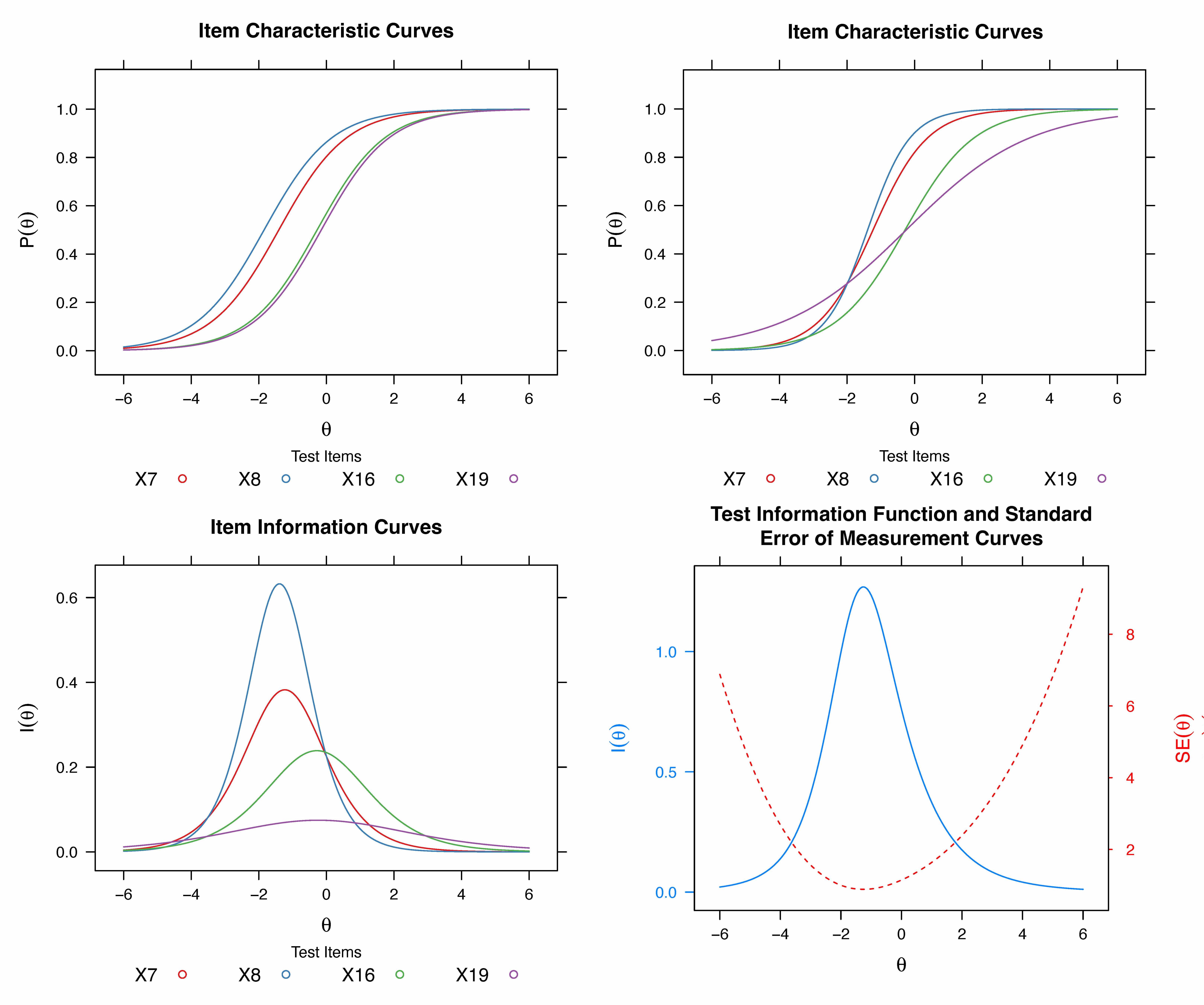
Figure 2: IRT Theory plots, taken from El-Hamamsy et al. (2022d)
(A - top left) Item Characteristic Curves for four items of equal discrimination (slope) and varying difficulty (using a 1-PL model on the cCTt test data). The item’s difficulty ($b_{i}$) is the x-value ($\theta$) where the ICC reaches a $y=0.5$ probability of answering correctly, and represents the number of standard deviations from the mean the question difficulty is. Items to the left of the graph are considered easier while items on the right are considered harder. According to De Ayala and Little (2022), “typical item and person locations fall within -3 to +3”, with easy items having scores below -2, average items having scores between -2 and +2 and hard items having scores above +2.
(B - top right) Item Characteristic Curves (ICC) for four items (blue, red, green, purple) of varying difficulty and discrimination (using a 2-PL model on cCTt test data). In this example, blue and red items are of equal difficulty $b_{i}$ ($y=0.5$ crossing) and relatively similar discrimination $a_{i}$, while items green and purple are of equal difficulty and varying discrimination. As the blue item is steeper, it has a higher discrimination than the red, green and purple items. According to De Ayala and Little (2022), reasonably good discrimination values range from approximately 0.8 to 2.5.
(C - bottom left) Item Information Curves (IICs) for the items in (B). The bell shaped curves represent the amount of information $I_{i}$ provided for each of the test’s items according to the student’s ability $\theta$. These IICs vary in both maximum value (dependent on the item’s discriminability, i.e. the ICC slope), and the x-value at which they reach it (the item’s difficulty). Here, the blue and red curves, as well as the green and purple curves, have the same difficulty (they both reach their maximum around x=-2 and x=0 respectively), but are of different discriminability: the blue item discriminates more than the red, the red more than the green and the green more than the purple (steeper ICC slope, and higher maximum IIC value).
(D - bottom right) Test Information Function (TIF, in blue) for the four items from Fig. 2 (B) and (C), and the standard error of measurement (SEM, in red). The TIF (blue) is the sum of the instrument’s IICs from Fig. 2 (B) and (C), while the SEM is the square root of the variance. The TIF shows that the instrument displays maximum information around -2 and provides more information in the low-medium ability range than in the high ability range. The SEM (red) is at its lowest where the test provides the most information (maximum of the TIF) and at its highest where the test provides the least information (minimum of the TIF).

Establishing student proficiency profiles.

As “an assessment is not an end in itself” and given that “it should contribute to promoting student learning (Pellegrino et al., 2016)” (Guggemos et al., 2022), proficiency profiles are established through IRT in order to improve the utility of the cCTt for researchers, educators and practitioners. The objective is to provide profiles “ranging from very low levels of proficiency to very high levels of proficiency”, which each “describ[ing] what students typically know and can do at [said]] level of proficiency” (OECD, 2017). These profiles are established as was done by Guggemos et al. (2022) for the CTt, by drawing inspiration from the approach employed by the OECD for the PISA assessments (OECD, 2014, 2017) and the fact that a student of a given ability “are increasingly more likely to complete tasks located at progressively lower points on the scale, and increasingly less likely to complete tasks located at progressively higher points on the scale” (OECD, 2017). Therefore, based on the outputs of IRT models, multiple proficiency levels are constructed with respect to the test’s item difficulties on the logit scale. To define the levels, the OECD proposed to consider proficiency levels of a width of 0.8 with the following criteria:

• Students of a given ability have a 62% chance of answering an item of said difficulty correctly

• Students at the bottom of a proficiency level (which is bounded by two difficulties on the logit scale) should have a 62% chance of answering the questions at the bottom of the level correctly, a 42% chance of answering the questions at the top of the level correctly, and an average 52% correct response rate for all the items in that level

• Students at the top of a proficiency level (which is bounded by two difficulties on the logit scale) should have a 62% chance of answering the questions at the top of the level correctly, a 78% chance of answering the questions at the bottom of the level correctly, and an average 70% correct response rate for all the items in that level

To achieve this therefore requires computing an adjusted difficulty per item, which for a 2PL model can be done using equation 1 , where $P_{i}$ represents the probability of answering an item correctly (and here should be equal to 0.62), $\theta$ represents the ability of the student to reach a probability $P_{i}$ of answering the item correctly, $b$ represents an item’s difficulty, $a$ represents the item’s discrimination.

$$\begin{split}P(\theta,a,b)=\frac{e^{a(\theta-b)}}{1+e^{a(\theta-b)}}\\ \Leftrightarrow 0.62(1+e^{a(\theta-b)})=e^{a(\theta-b)}\\ \Leftrightarrow\log{\frac{0.62}{0.38}}=a(\theta-b))\\ \Leftrightarrow\theta=\frac{1}{a}\log{\frac{0.62}{0.38}}+b\\ \end{split}$$ (1)

2.3.3 Differential Item Functioning

Differential Item Functioning (DIF) is statistical approach that is usually employed to determine whether there are biases in response patterns between groups for certain items (e.g. according to gender as done by Rachmatullah et al., 2022; Sovey et al., 2022 or countries as done by Rachmatullah et al., 2022). Similarly to IRT, DIF attempts to determine whether members of different groups who have the same underlying ability have a different probability of answering a question correctly. DIF therefore indicates whether an instruments’ items are “consistent and fair for all participants” and is an indicator of the validity of the instrument. More specifically, provided responses of students from different groups (e.g. gender or demographics), an item that is identified as being DIF should be reformulated in order for students of a given ability in both groups have the same probability of answering the questions correctly.

In the present context we employ DIF to determine whether i) there are differences in the response patterns between students in grades 3-4 and grades 5-6, and whether grade-specific IRT models should be employed instead of a single model, and ii) the instrument is fair with respect to gender as instruments such as these are often employed to determine whether gender gaps exist and whether interventions help address them given the lack of diversity in computing-related fields (Rachmatullah et al., 2022). While it would have been interesting to establish fairness in terms of socio-economic status, this type of information is considered sensitive in the region.

The DIF analysis was conducted with the following parameters:

• the IRT model (1-PL, 2-PL, 3-PL or 4-PL) that is most appropriate for the four grades

• purification, an iterative approach that removes items flagged as DIF before repeating the search to ensure that all DIF items are identified (Magis et al., 2011)

• Benjamini-Hochberg p-value correction to reduce the false discovery rate due to multiple comparisons

• multiple DIF detection methods: the Generalised Mantel-Haenszel $\chi^{2}$ statistic, the generalised logistic regression Likelihood-ratio test (LRT), and the generalised Lord’s $\chi^{2}$ statistic (Magis et al., 2020).

3 Results

3.1 Score distribution and score normalisation for equivalency scales

3.1.1 Differences according to grade

The distribution of scores obtained per student and grade can be seen in Fig. 3 with the descriptive statistics being provided in Table 4. The skew and kurtosis values are within the acceptable range for normal univariate distribution according to (Gravetter et al., 2020) although the skew to the left increases between grades 3, 4 and 5-6. A one-way ANOVA reveals significant differences according to students’ grades ($F(3)=95$, $p<0.0001$). Dunn’s test for multiple comparisons in Table 5 indicates that there are significant differences between all grades, except between grades 5 and 6 where a plateau appears to have been reached.

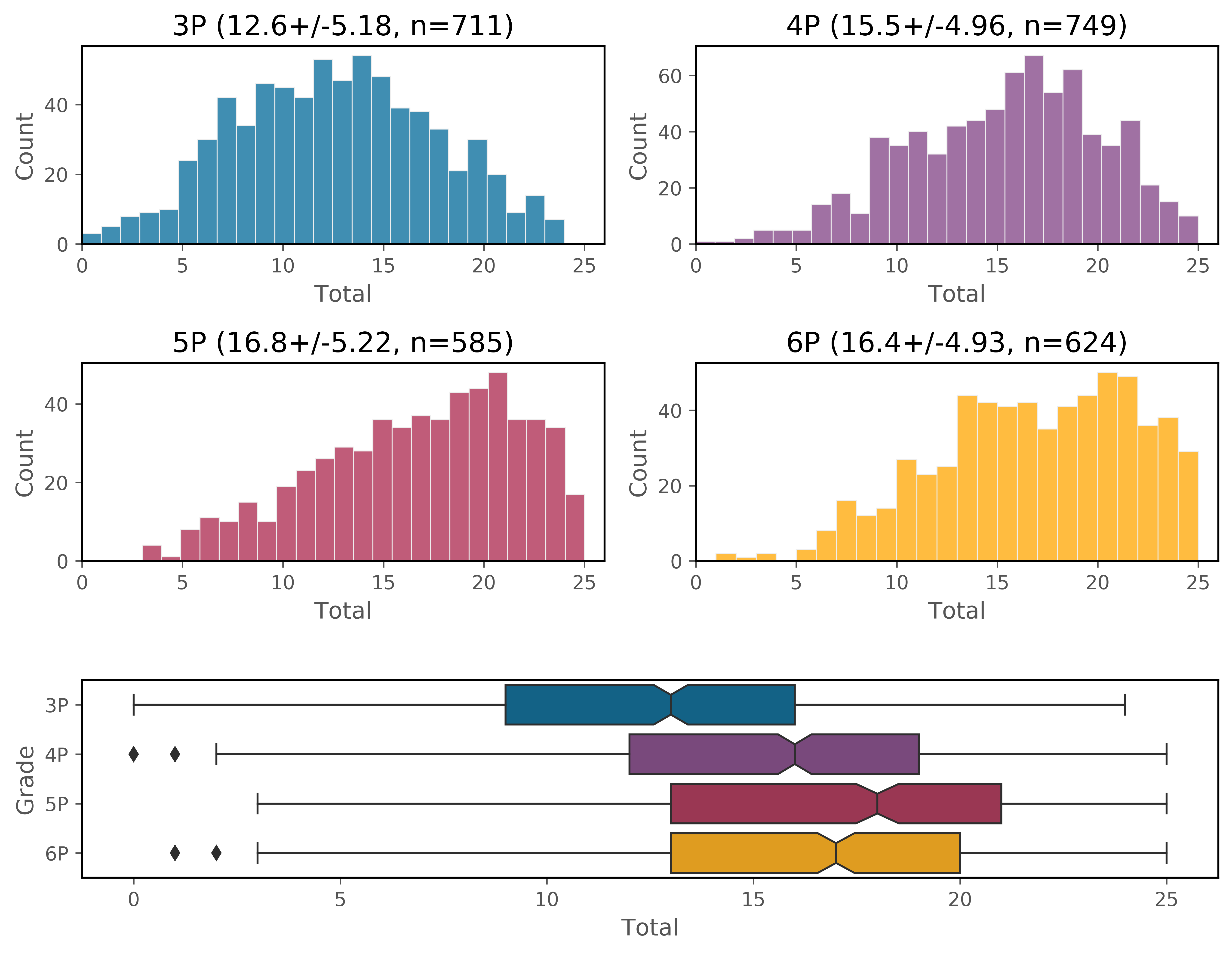
Figure 3: Distribution of scores across grades

Table 4: Descriptive statistics of the cCTt per grade. Please note that acceptable limits to prove normal univariate distribution are $[-2;+2]$ for Skew and $[-7;+7]$ for Kurtosis (Gravetter et al., 2020), with values close to 0 being desirable.

	N	Mean	Std. error of the mean	Std. deviation	Skew	Kurtosis	Min	Max
3P	711	12.6	0.194	5.18	0.0206	-0.593	0	24
4P	749	15.5	0.181	4.96	-0.354	-0.408	0	25
5P	585	16.8	0.216	5.22	-0.489	-0.548	3	25
6P	624	16.4	0.197	4.93	-0.416	-0.461	1	25

Table 5: Dunn’s test for multiple comparisons between grades with Benjamini-Hochberg p-value correction (minimum Cohen’s $D=0.128$ to achieve a statistical power of 0.8).

	3P	4P	5P
4P	$\Delta=2.87$pts, $p=0.0$, $D=0.566$
5P	$\Delta=4.22$pts, $p=0.0$, $D=0.812$	$\Delta=1.35$pts, $p=0.0$, $D=0.266$
6P	$\Delta=3.80$pts, $p=0.0$, $D=0.751$	$\Delta=0.93$pts, $p=0.0013$, $D=0.188$	$\Delta=0.423$pts, $p=0.1345$, $D=0.083$ (n.s.)

Using a normalised scoring approach (Relkin, 2022), Table 6 provides the percentile to which each student belongs according to the score obtained (after z-scoring) and their grade.

Table 6: Normalised z-scoring and percentiles according to the score obtained on the cCTt and grade. Z-scores are provided with 3 significant digits.

cCTt Score	3P		4P		5P		6P
	Z-Score	Percentile	Z-Score	Percentile	Z-Score	Percentile	Z-Score	Percentile
0	-2.440	0.0	-3.1300	0.0	-3.2300	0.0	-3.3300	0.0
1	-2.240	0.0	-2.9200	0.0	-3.0400	0.0	-3.1300	0.0
2	-2.050	1.0	-2.7200	0.0	-2.8400	0.0	-2.9300	0.0
3	-1.860	2.0	-2.5200	0.0	-2.6500	0.0	-2.7200	0.0
4	-1.660	4.0	-2.3200	1.0	-2.4600	0.0	-2.5200	0.0
5	-1.470	6.0	-2.1200	2.0	-2.2700	1.0	-2.3200	1.0
6	-1.280	10.0	-1.9200	3.0	-2.0800	3.0	-2.1100	2.0
7	-1.090	15.0	-1.7100	5.0	-1.8900	5.0	-1.9100	3.0
8	-0.892	20.0	-1.5100	7.0	-1.6900	7.0	-1.7100	6.0
9	-0.699	26.0	-1.3100	10.0	-1.5000	9.0	-1.5100	8.0
10	-0.506	32.0	-1.1100	15.0	-1.3100	11.0	-1.3000	11.0
11	-0.313	39.0	-0.9060	20.0	-1.1200	15.0	-1.1000	15.0
12	-0.120	45.0	-0.7040	25.0	-0.9280	19.0	-0.8970	19.0
13	0.073	52.0	-0.5020	30.0	-0.7360	24.0	-0.6940	24.0
14	0.266	59.0	-0.3010	36.0	-0.5450	29.0	-0.4910	31.0
15	0.459	67.0	-0.0989	42.0	-0.3530	34.0	-0.2880	38.0
16	0.652	73.0	0.1030	49.0	-0.1620	40.0	-0.0852	45.0
17	0.845	78.0	0.3050	58.0	0.0301	46.0	0.1180	51.0
18	1.040	83.0	0.5070	66.0	0.2220	52.0	0.3210	57.0
19	1.230	87.0	0.7080	74.0	0.4130	59.0	0.5240	64.0
20	1.420	90.0	0.9100	80.0	0.6050	67.0	0.7270	71.0
21	1.620	94.0	1.1100	85.0	0.7970	74.0	0.9300	79.0
22	1.810	96.0	1.3100	90.0	0.9880	82.0	1.1300	86.0
23	2.000	98.0	1.5200	95.0	1.1800	88.0	1.3400	92.0
24	2.200	99.0	1.7200	97.0	1.3700	94.0	1.5400	97.0
25	2.390	100.0	1.9200	99.0	1.5600	98.0	1.7400	99.0

3.1.2 Differences according to gender

Given that the cCTt’s items are not biased with respect to gender (see section 3.3) we check whether there are significant differences in terms of performance between boys and girls. Therefore, considering the data for grades 3-6, a one-way ANOVA indicates that there are significant differences according to gender ($F(1)=5.45$, $p=0.0197$), although the effect size for the latter is too low to conclude with the given sample size (Cohen’s $D=0.09$, with $D_{min}=0.108$ for the sample). However a two-way ANOVA indicates an interaction effect between the gender and grade ($F(7)=42$, $p<0.0001$) with the differences between genders being significant in grade 3, but not in grades 4, 5 and 6 (see Table 7).

Table 7: Dunn’s test for multiple comparisons between genders according to grade (minimum Cohen’s $D=0.147$ to achieve a statistical power of 0.8). $\Delta$ here is the difference between the mean score obtained by boys and mean score obtained by girls

3P	4P	5P	6P
(Boys $>$ Girls) $\Delta=0.829pts$ , $p=0.0317$, $D=0.161$	(n.s.) $\Delta=0.728pts$ , $p=0.1053$, $D=0.147$	(n.s.) $\Delta=0.147pts$, $p=0.8272$, $D=0.028$	(n.s.) $\Delta=0.461pts$, $p=0.4592$, $D=0.094$

3.2 Classical Test Theory for cCTt sample dependent reliability

Fig. 4 reports the Classical Test Theory analysis results (difficulty indices and point biserial correlations) for all questions according to the students’ grade. Starting with item difficulty indices, the trends observed for students in grades 3 and 4 appear consistent with those observed in grades 5 and 6. The students also appear to perform better in grades 5 and 6 on the individual items, to the point where there are no items which are too difficult, but a larger number which are too easy compared to grades 3-4 (see Fig. 4). When considering the point biserial correlation, items where students score nearly perfectly also have low point biserial correlations, with errors on these items not being representative of the students’ overall performance on the test, and likely due to oversights on their part. Finally, when considering the reliability provided by Cronbach’s $\alpha$, the cCTt exhibits good reliability for each grade ($\alpha_{3P}=0.84$, $\alpha_{4P}=0.84$, $\alpha_{5P}=0.83$, $\alpha_{6P}=0.82$). Additionally, when computing the drop $\alpha$ per question, i.e. the reliability of the instrument should an item be removed, the value is always lower than the overall reliability for that grade, indicating that removing an item will not improve the reliability of the instrument.

Taking all of these elements into account, it would appear that the following number of questions could be revised to improve the validity of the instrument:

• 5 in grade 3: Q1 and Q2 which are too easy, Q17, Q24 and Q25 which are too hard

• 5 in grade 4: Q1, Q2, and Q6 which are too easy, Q17 and Q24 which are too hard

• 7 in grade 5: Q1-Q4, Q6, Q8, Q9 which are too easy, notably considering that Q1, Q2 and Q4 have low point-biserial correlations

• 6 in grade 6: Q1-Q2, Q4, and Q6, Q8, Q9 which are too easy, notably considering that Q1, Q2 and Q4 have low point-biserial correlations

While the two first items of the instrument would be the most important to revise, these could be considered as a means for the students to familiarise with the test and could simply be removed from the final score. This is particularly relevant for students in grades 5-6 as the point-biserial correlation is below the acceptable limit for these grades. Furthermore, given the mastery that students appear to have on sequences in grades 5-6, and the scores obtained on more advanced CT-concepts, it may be relevant to introduce more questions on advanced CT-concepts in their stead.

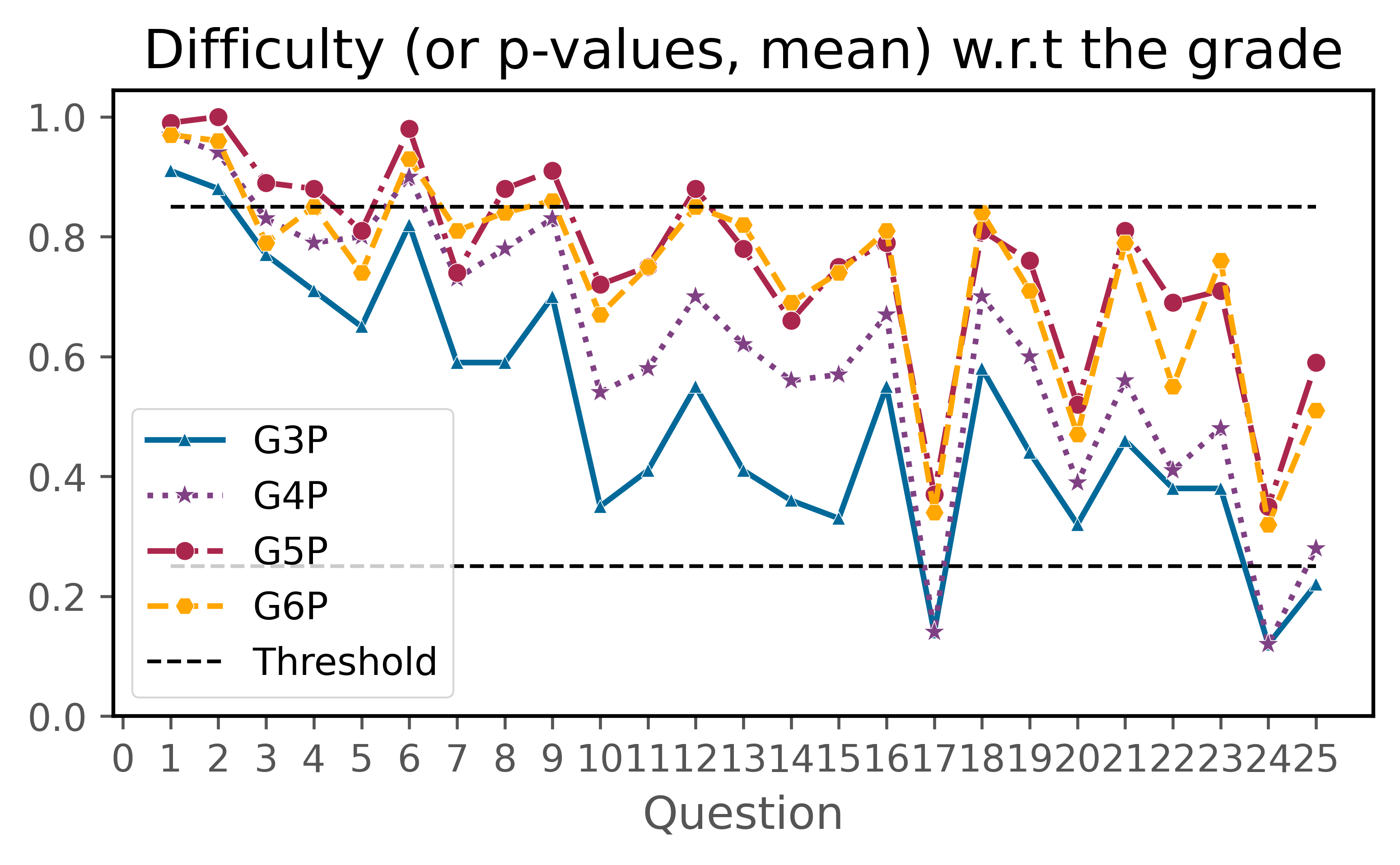
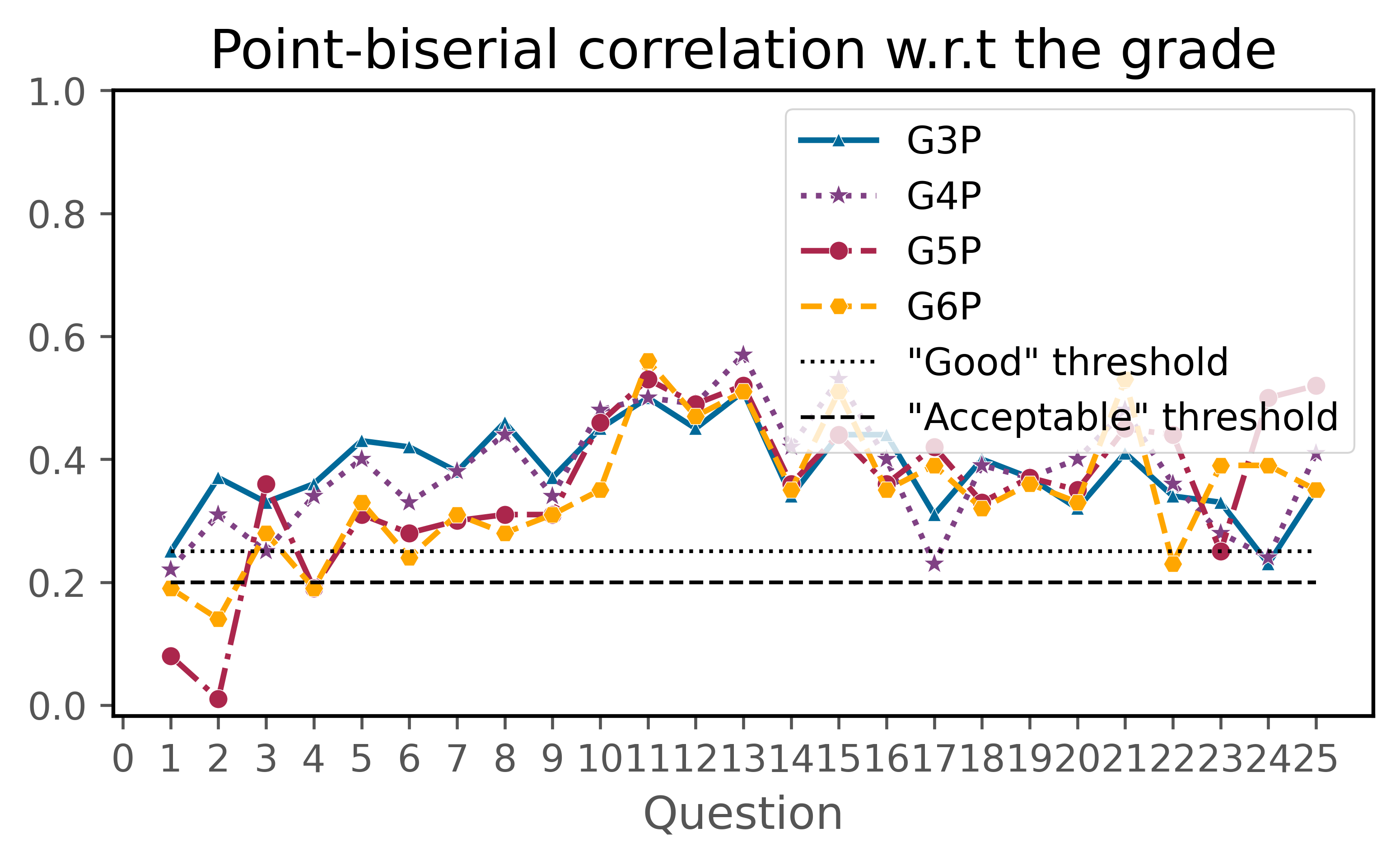
Figure 4: Classical Test Theory - Item Difficulty Index (left) and Point-biserial correlation (right). Please note that items with a difficulty index above the 0.85 threshold are considered too easy while items below the 0.25 threshold are considered too difficult. Similarly, items with a point-biserial correlation above the 0.2 threshold are considered acceptable while those above 0.25 are considered good.

3.3 Differential Item Function for cCTt gender-fairness

Given the importance of having generalisable instruments that are fair towards all groups of participants, we employ Differential Item Functioning (DIF) to investigate whether there the cCTt’s items are biased with respect to gender. The results in Table 8 indicate that all items are not flagged DIF at least two out of three time, with only 3/25 items (Q8, Q14, Q19) being flagged by one of the three methods as DIF with a negligeable effect. As such, we can conclude that there are no significantly DIF items in the cCTt and that the cCTt can be considered fair with respect to gender.

Table 8: Differential Item Functioning between genders (girls = focal). Abbreviations: Stat. = statistic, Adj. P. = adjusted p-value using Benjamini-Hochberg p-value correction).

	Mantel-Haenszel (M.-H.) $\chi^{2}$			Logistic Regression Likelihood Ratio Test (LRT)				Generalized Lord’s $\chi^{2}$		Synthesis
	Stat.	Adj. P	Effect size (ETS Delta scale)	Stat.	Adj. P	$R^{2}$ (Nagelkerke’s $R^{2}$)	Effect size (Jodoin & Gierl)	Stat	Adj. P	M.-H.	LRT	Lord	#DIF
Q1	1.02	0.3131	Negligeable	2.32	0.7873	0.0027	Negligeable	1.44	0.757	NoDIF	NoDIF	NoDIF	0/3
Q2	0.13	0.722	Negligeable	0.92	0.9237	0.0008	Negligeable	1.51	0.757	NoDIF	NoDIF	NoDIF	0/3
Q3	0.74	0.389	Negligeable	1.77	0.7873	0.0006	Negligeable	2.05	0.757	NoDIF	NoDIF	NoDIF	0/3
Q4	0.00	0.9714	Negligeable	0.30	0.9893	0.0001	Negligeable	0.81	0.7944	NoDIF	NoDIF	NoDIF	0/3
Q5	0.42	0.5166	Negligeable	1.22	0.9069	0.0004	Negligeable	1.46	0.757	NoDIF	NoDIF	NoDIF	0/3
Q6	0.18	0.6721	Negligeable	2.21	0.7873	0.0007	Negligeable	3.11	0.757	NoDIF	NoDIF	NoDIF	0/3
Q7	0.02	0.8977	Negligeable	0.34	0.9893	0.0001	Negligeable	1.68	0.757	NoDIF	NoDIF	NoDIF	0/3
Q8	5.18	0.0228*	Negligeable	6.24	0.4432	0.0018	Negligeable	4.65	0.6103	DIF	NoDIF	NoDIF	1/3
Q9	0.00	0.9773	Negligeable	0.16	0.9893	0.0001	Negligeable	1.08	0.7666	NoDIF	NoDIF	NoDIF	0/3
Q10	0.38	0.5365	Negligeable	0.09	0.9893	0	Negligeable	1.83	0.757	NoDIF	NoDIF	NoDIF	0/3
Q11	2.49	0.1147	Negligeable	1.65	0.7873	0.0004	Negligeable	1.93	0.757	NoDIF	NoDIF	NoDIF	0/3
Q12	1.14	0.2852	Negligeable	3.55	0.7154	0.0009	Negligeable	0.33	0.8661	NoDIF	NoDIF	NoDIF	0/3
Q13	0.60	0.4394	Negligeable	2.17	0.7873	0.0005	Negligeable	6.21	0.3735	NoDIF	NoDIF	NoDIF	0/3
Q14	6.14	0.0132*	Negligeable	5.81	0.4432	0.0017	Negligeable	2.12	0.757	DIF	NoDIF	NoDIF	1/3
Q15	2.27	0.1322	Negligeable	1.64	0.7873	0.0004	Negligeable	0.30	0.8661	NoDIF	NoDIF	NoDIF	0/3
Q16	0.00	0.9787	Negligeable	0.14	0.9893	0	Negligeable	1.26	0.757	NoDIF	NoDIF	NoDIF	0/3
Q17	1.86	0.1721	Negligeable	2.14	0.7873	0.0007	Negligeable	1.46	0.757	NoDIF	NoDIF	NoDIF	0/3
Q18	0.23	0.6282	Negligeable	0.82	0.9237	0.0002	Negligeable	3.04	0.757	NoDIF	NoDIF	NoDIF	0/3
Q19	6.21	0.0127*	Negligeable	6.51	0.4432	0.0019	Negligeable	8.95	0.1426	DIF	NoDIF	NoDIF	1/3
Q20	2.65	0.1037	Negligeable	2.07	0.7873	0.0006	Negligeable	0.29	0.8661	NoDIF	NoDIF	NoDIF	0/3
Q21	3.10	0.0781	Negligeable	3.52	0.7154	0.001	Negligeable	3.60	0.757	NoDIF	NoDIF	NoDIF	0/3
Q22	1.04	0.3082	Negligeable	1.06	0.9207	0.0003	Negligeable	1.21	0.757	NoDIF	NoDIF	NoDIF	0/3
Q23	0.04	0.838	Negligeable	0.02	0.9893	0	Negligeable	0.97	0.7707	NoDIF	NoDIF	NoDIF	0/3
Q24	1.82	0.1769	Negligeable	0.48	0.9893	0.0001	Negligeable	0.64	0.8232	NoDIF	NoDIF	NoDIF	0/3
Q25	2.06	0.151	Negligeable	5.29	0.4432	0.0015	Negligeable	9.76	0.1426	NoDIF	NoDIF	NoDIF	0/3

Please note that the DifR package does not provide the effect size for Lord’s $\chi^{2}$ statistic.

3.4 Item Response Theory (IRT) for cCTt sample-agnostic reliability

3.4.1 Applicability of IRT

We employed Confirmatory Factor Analysis using the weighted diagonally least squares estimator to determine whether the instrument could be considered as unidimensional (Kong and Lai, 2022). We did not meet the goodness of fit requirements for all grades on all criteria with the robust estimator, in particular for grade 5. This is unsurprising as “violations of unidimensionality and local independence are always present in the real measures” (Rajlic, 2019). Research has found that with violations of unidimensionality, i) there may be an overestimation of the discrimination parameter, ii) with little impact on the difficulty estimation, and iii) that the impact on the estimated parameters is smaller the closer we are to the unidimensionality criteria (Kahraman, 2013; Rajlic, 2019). As the level of mis-specification is low, notably when removing Q2 from the model (which was the item that the Classical Test Theory most often indicated as needing revision), and all factor loadings exceed 0.3 and are significant, we can proceed with the IRT analysis which we conduct without the first block of questions (see Table 9).

Table 9: cCTt Unidimensional CFA Robust Fit Indices

	Q1-Q25				Q1 + Q3-Q25
	3P	4P	5P	6P	3P	4P	5P	6P
df	275	275	275	275	735.526	939.859	368.787	399.773
$\chi^{2}$	805	992	667	420	252	252	252	252
p-$\chi^{2}$	0	0	0	0	0	0	0	0
$\chi^{2}$/df	2.93	3.61	2.43	1.53	2.92	3.73	1.46	1.59
CFI	0.897	0.874	0.819	0.924	0.9	0.877	0.939	0.926
TLI	0.888	0.863	0.803	0.917	0.891	0.866	0.933	0.918
RMSEA	0.052	0.059	0.064	0.038	0.052	0.06	0.036	0.04
RMSEA upper 90% ci	0.048	0.055	0.064	0.031	0.048	0.056	0.028	0.033
RMSEA lower 90% ci	0.056	0.063	0.070	0.046	0.056	0.065	0.044	0.048
SRMR	0.09	0.107	0.126	0.112	0.088	0.106	0.113	0.107
Factor Loading	$\beta>0.399$	$\beta>0.392$	$\beta>0.309$	$\beta>0.303$	$\beta>0.4$	$\beta>0.394$	$\beta>0.340$	$\beta>0.424$
estimates				except $\beta_{Q4}=0.292$			except $\beta_{Q1}=0.248$	except $\beta_{Q4}=0.292$
Factor Loading	$p<0.001$	$p<0.001$	$p<0.001$	$p<0.001$	$p<0.001$	$p<0.001$	$p<0.001$	$p<0.001$
p-values				except $p_{Q2}=0.015$

3.4.2 Identifying the most appropriate model

The 3-PL model did not converge to a stable solution for students in grades 3, 4 and 6, and the 4-PL model did not converge at all for any of the grades. As the objective is to compare the instruments, and use a single model type for the analysis, we fit the 1PL and 2PL models for each grade. Using ANOVA to compare the 1PL and 2PL models indicates that the 2PL model significantly improves the fit in all cases (see Table 10). Yen’s Q3 statistic (Yen, 1984) to measure local independence indicates that none of the pairs of item residuals have a high correlation (all values $<0.2$) for grades 3, 5 and 6, and that just 2 items have a statistic between 0.2 and 0.3 (acceptable) for students in grade 4. We can thus consider that local independence is not violated.

Table 10: cCTt (excluding item Q2) IRT Model comparison using ANOVA for each grade

Grade	Model	AIC	BIC	Log Likelihood	LRT	df	p-value
3P	1PL	18636.07	18750.24	-9293.03
	2PL	18592.46	18811.66	-9248.23	89.61	23	$<0.001$
4P	1PL	18081.03	18196.50	-9015.52
	2PL	17969.57	18191.27	-8936.79	157.46	23	$<0.001$
5P	1PL	11708.63	11817.92	-5829.31
	2PL	11624.36	11834.20	-5764.18	130.26	23	$<0.001$
6P	1PL	12967.41	13078.31	-6458.70
	2PL	12865.30	13078.23	-6384.65	148.11	23	$<0.001$

3.4.3 Identifying differences between students in grades 3-4 versus 5-6 with Differential Item Functioning

To determine whether there are differences in response patterns between grades 3-4 and 5-6 we employ Differential Item Functioning (DIF) for a 2-PL model. The results in Table 11 and Fig. 5 indicate that all the items were flagged at least two our of three times as DIF, with 16/25 being flagged by all three detection methods as DIF. This would indicate that there are differences in difficulty or discriminability among the questions depending on the grades the students are in. As such, we are interested in comparing how the IRT parameters vary across grades.

Table 11: Differential Item Functioning between grades 3-4 (reference) and grades 5-6 (focal). Abbreviations: Stat. = statistic, Adj. P. = adjusted p-value using Benjamini-Hochberg p-value correction).

Mantel-Haenszel (M.-H.) $\chi^{2}$

Logistic Regression Likelihood Ratio Test (LRT)

Generalized Lord’s $\chi^{2}$

Synthesis

Stat.

Adj. P

Effect size (ETS Delta scale)

Stat.

Adj. P

$R^{2}$ (Nagelkerke’s $R^{2}$)

Effect size (Jodoin & Gierl)

Stat

Adj. P

M.-H.

LRT

Lord

#DIF

Q1

61.4

0***

Large

9.1

0.0113*

0.0096

Negligible

8.3

0.0217*

DIF

DIF

DIF

3/3

Q2

101.7

0***

Large

0.1

0.9651

0.0001

Negligible

25.8

0***

DIF

No DIF

DIF

2/3

Q3

95.1

0***

Large

49.3

0***

0.0118

Negligible

30.4

0***

DIF

DIF

DIF

3/3

Q4

134

0***

Large

0.2

0.9506

0

Negligible

29.0

0***

DIF

No DIF

DIF

2/3

Q5

118.1

0***

Large

37.2

0***

0.008

Negligible

73.1

0***

DIF

DIF

DIF

3/3

Q6

130.3

0***

Large

9.7

0.009**

0.0027

Negligible

15.7

0.0008***

DIF

DIF

DIF

3/3

Q7

137.9

0***

Large

21.7

0***

0

Negligible

38.0

0***

DIF

DIF

DIF

3/3

Q8

186.9

0***

Large

15.1

0.0006***

0.0033

Negligible

28.9

0***

DIF

DIF

DIF

3/3

Q9

113

0***

Large

81.5

0***

0.0214

Negligible

10.3

0.009**

DIF

DIF

DIF

3/3

Q10

117.6

0***

Large

181.6

0***

0

Negligible

31.3

0***

DIF

DIF

DIF

3/3

Q11

133

0***

Large

148.6

0***

0

Negligible

19.0

0.0002***

DIF

DIF

DIF

3/3

Q12

157.8

0***

Large

175.7

0***

0.0398

Moderate

1.7

0.4754

DIF

DIF

No DIF

2/3

Q13

149.9

0***

Large

244.8

0***

0

Negligible

13.7

0.0019**

DIF

DIF

DIF

3/3

Q14

115.8

0***

Large

117.6

0***

0

Negligible

18.5

0.0002***

DIF

DIF

DIF

3/3

Q15

162.4

0***

Large

174.7

0***

0

Negligible

16.7

0.0005***

DIF

DIF

DIF

3/3

Q16

237.2

0***

Large

77.0

0***

0.0169

Negligible

11.6

0.0052**

DIF

DIF

DIF

3/3

Q17

251.1

0***

Large

55.0

0***

0

Negligible

0.7

0.7053

DIF

DIF

No DIF

2/3

Q18

245.9

0***

Large

104.1

0***

0.0238

Negligible

5.0

0.1082

DIF

DIF

No DIF

2/3

Q19

271.2

0***

Large

86.3

0***

0.577

Large

4.9

0.1082

DIF

DIF

No DIF

2/3

Q20

162.9

0***

Large

44.1

0***

0

Negligible

34.7

0***

DIF

DIF

DIF

3/3

Q21

253

0***

Large

247.7

0***

0.5883

Large

3.9

0.1663

DIF

DIF

No DIF

2/3

Q22

193.9

0***

Large

88.8

0***

0

Negligible

3.1

0.2435

DIF

DIF

No DIF

2/3

Q23

271.3

0***

Large

226.4

0***

0

Negligible

14.8

0.0012**

DIF

DIF

DIF

3/3

Q24

225.4

0***

Large

45.9

0***

0.5763

Large

9.6

0.0121*

DIF

DIF

DIF

3/3

Q25

277

0***

Large

104.9

0***

0

Negligible

1.4

0.5176

DIF

DIF

No DIF

2/3

Please note that the DifR package does not provide the effect size for Lord’s $\chi^{2}$ statistic.

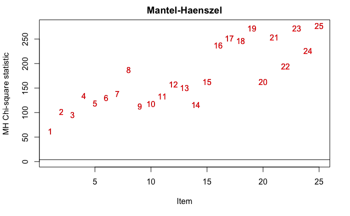
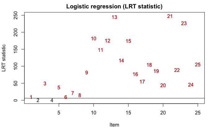
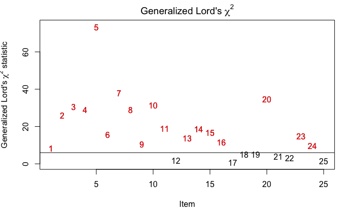
Figure 5: Results of the DIF according to the detection method employed. The higher the statistic for a given item, the more the item is DIF between grades 3-4 and 5-6.

3.4.4 Comparing the instruments’ grade-specific IRT models’ properties

To gain better insight into how the properties of the test differ according to grade, we compare the IRT models for each of the grades in terms of difficulty and discrimination indices. The grade specific Item Response Theory models parameters are provided in Table 12. Fig. 6 shows the Item Characteristic Curves (ICCs), Fig. 7 the Item Information Curves (IICs) and Fig. 8 the Test Information Functions and Standard Error of Measurements (TIFs). The average item discrimination for all tests is in the upper-moderate range with the minimum value in the upper-low range, and the maximum value in the very high range. While the distribution in item discrimination does not differ significantly according to grade (one-way ANOVA $F(3)=0.77$, $p=0.51$), the distribution of item difficulties does ($F(3)=7.52$, $p=0.00015$). Indeed, on average, the results would appear to indicate that the cCTt is easier the older the students are, and can be considered as medium-high for grade 3 students, medium-low for grade 4 students, and easy for students in grades 5-6. Dunn’s test for multiple comparisons with Benjamini-Hochberg p-value corrections is used to determine between which groups these differences are significant, all the while accounting for the minimum effect size required to meet a statistical power of 0.8. The test indicates that the differences are significant between grades 3 and 5 ($\Delta=1.35$, $p=0.0007$, $D=1.22$), and 3 and 6 ($\Delta=1.33$, $p=0.0007$, $D=1.15$). This is confirmed by the Test Information Function, which indicates that the cCTt provides the most information for medium ability students in grades 3, while it provides more information for medium-low ability students in grades 4-6.

Table 12: 2-PL IRT Difficulty (Dffclt) and Discrimination (Dscrmn) Parameters per grade. Please note that we also provide the equivalent difficulty for a 62% of correct response probability for the student proficiency levels construction.

	3P			4P			5P			6P
	Dffclt	Dscrmn	Dffclt 62%	Dffclt	Dscrmn	Dffclt 62%	Dffclt	Dscrmn	Dffclt 62%	Dffclt	Dscrmn	Dffclt 62%
Q1	-2.550	1.085	-2.099	-2.950	1.538	-2.632	-3.570	1.158	-3.147	-3.570	1.158	-3.236
Q3	-1.440	1.006	-0.954	-2.175	0.806	-1.568	-2.366	0.944	-1.848	-2.366	0.944	-1.240
Q4	-1.055	0.997	-0.564	-1.606	0.969	-1.101	-3.048	0.652	-2.297	-3.048	0.652	-2.410
Q5	-0.618	1.304	-0.242	-1.329	1.414	-0.983	-1.462	1.135	-1.031	-1.462	1.135	-0.770
Q6	-1.278	1.753	-0.998	-2.030	1.434	-1.689	-2.754	1.715	-2.468	-2.754	1.715	-2.500
Q7	-0.430	1.033	0.044	-1.073	1.161	-0.651	-1.191	0.825	-0.598	-1.191	0.825	-1.268
Q8	-0.367	1.414	-0.021	-1.148	1.596	-0.841	-1.793	1.255	-1.403	-1.793	1.255	-1.639
Q9	-0.924	1.119	-0.487	-1.650	1.206	-1.244	-2.498	1.049	-2.031	-2.498	1.049	-1.649
Q10	0.572	1.416	0.917	-0.174	1.511	0.150	-0.779	1.348	-0.415	-0.779	1.348	-0.221
Q11	0.304	1.691	0.593	-0.285	1.833	-0.018	-0.773	1.941	-0.521	-0.773	1.941	-0.578
Q12	-0.186	1.480	0.145	-0.723	1.933	-0.470	-1.315	2.649	-1.130	-1.315	2.649	-1.031
Q13	0.316	1.776	0.592	-0.375	2.432	-0.174	-0.883	2.059	-0.645	-0.883	2.059	-0.825
Q14	0.697	0.940	1.218	-0.241	1.253	0.150	-0.630	1.048	-0.163	-0.630	1.048	-0.470
Q15	0.669	1.432	1.011	-0.242	1.966	0.007	-0.783	1.673	-0.491	-0.783	1.673	-0.494
Q16	-0.233	1.192	0.178	-0.801	1.065	-0.341	-1.150	1.233	-0.753	-1.150	1.233	-1.046
Q17	2.075	1.076	2.530	2.367	0.854	2.940	0.634	1.387	0.987	0.634	1.387	1.191
Q18	-0.364	1.026	0.113	-1.004	1.042	-0.534	-1.510	1.018	-1.029	-1.510	1.018	-1.287
Q19	0.289	0.950	0.804	-0.510	0.914	0.025	-1.094	1.065	-0.634	-1.094	1.065	-0.524
Q20	1.027	0.817	1.626	0.492	1.075	0.948	0.028	1.173	0.446	0.028	1.173	0.789
Q21	0.163	1.048	0.630	-0.236	1.305	0.140	-1.327	1.415	-0.981	-1.327	1.415	-0.850
Q22	0.664	0.835	1.250	0.467	0.939	0.988	-0.698	1.276	-0.314	-0.698	1.276	0.727
Q23	0.648	0.834	1.235	0.130	0.679	0.851	-1.708	0.565	-0.842	-1.708	0.565	-0.762
Q24	2.801	0.787	3.423	2.462	0.926	2.991	0.658	1.775	0.934	0.658	1.775	1.144
Q25	1.467	1.061	1.928	0.955	1.245	1.349	-0.180	1.517	0.142	-0.180	1.517	0.514
M	0.094	1.170	0.536	-0.487	1.296	-0.071	-1.258	1.328	-0.843	-1.258	1.328	-0.768
SD	1.155	0.296	1.193	1.274	0.427	1.314	1.059	0.468	1.009	1.059	0.468	1.115
Min	-2.550	0.787	-2.099	-2.950	0.679	-2.632	-3.570	0.565	-3.147	-3.570	0.565	-3.236
25%	-0.477	0.986	-0.076	-1.193	0.962	-0.876	-1.730	1.049	-1.199	-1.730	1.049	-1.273
50%	0.226	1.069	0.593	-0.443	1.225	-0.096	-1.170	1.244	-0.699	-1.170	1.244	-0.798
75%	0.665	1.415	1.222	-0.098	1.518	0.325	-0.755	1.556	-0.390	-0.755	1.556	-0.408
MAX	2.801	1.776	3.423	2.462	2.432	2.991	0.658	2.649	0.987	0.658	2.649	1.191

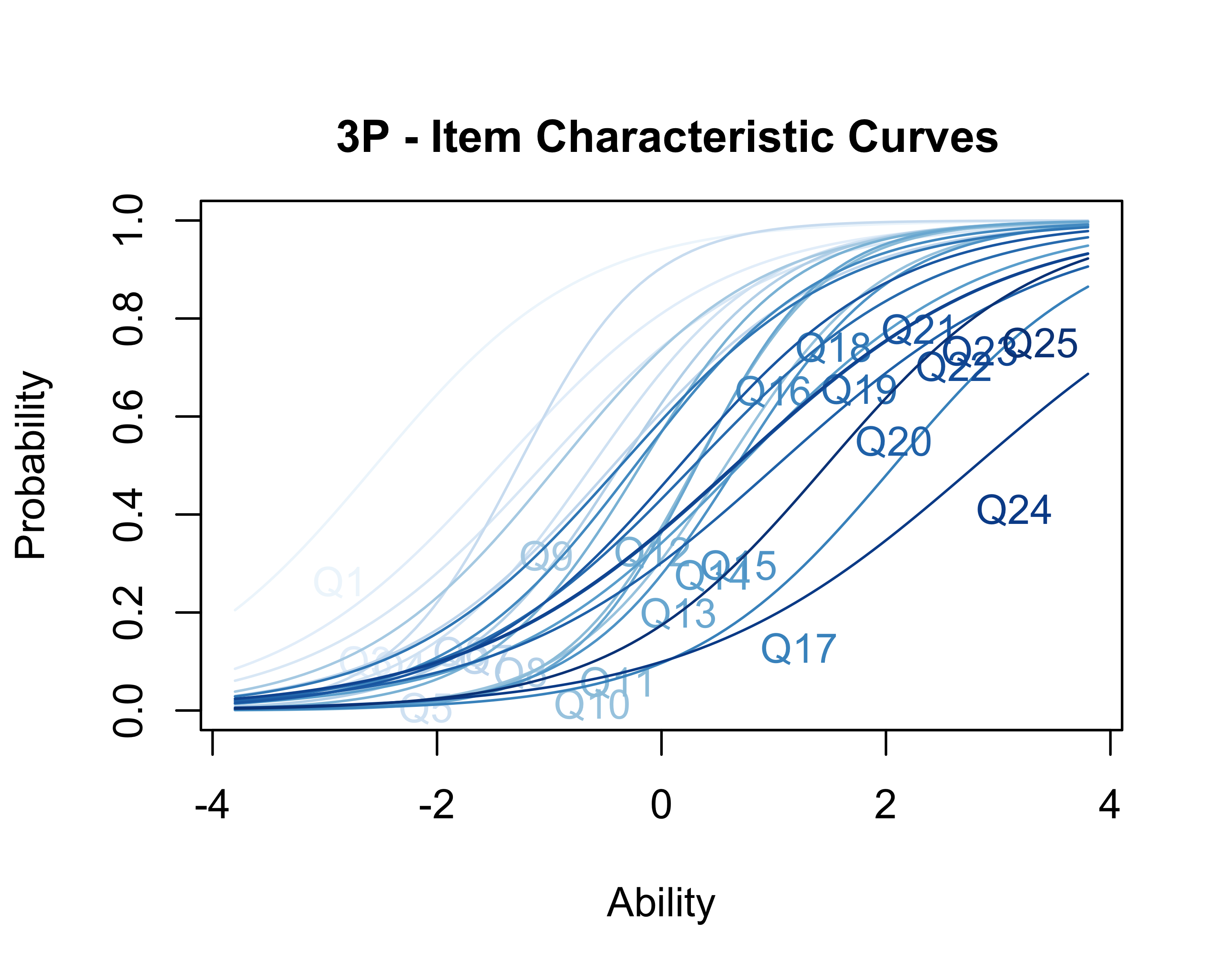
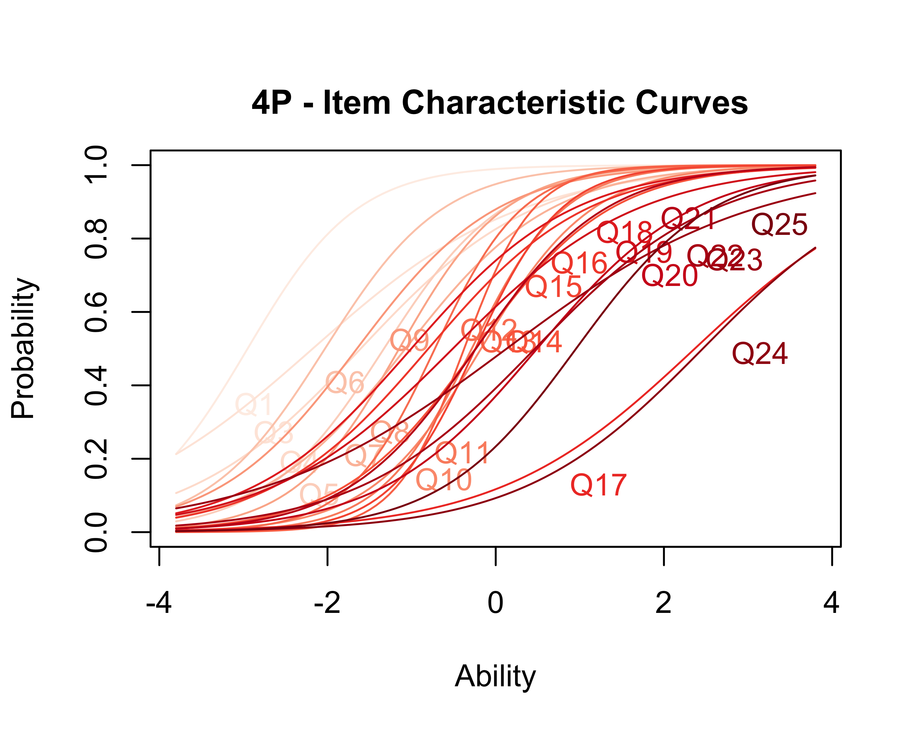
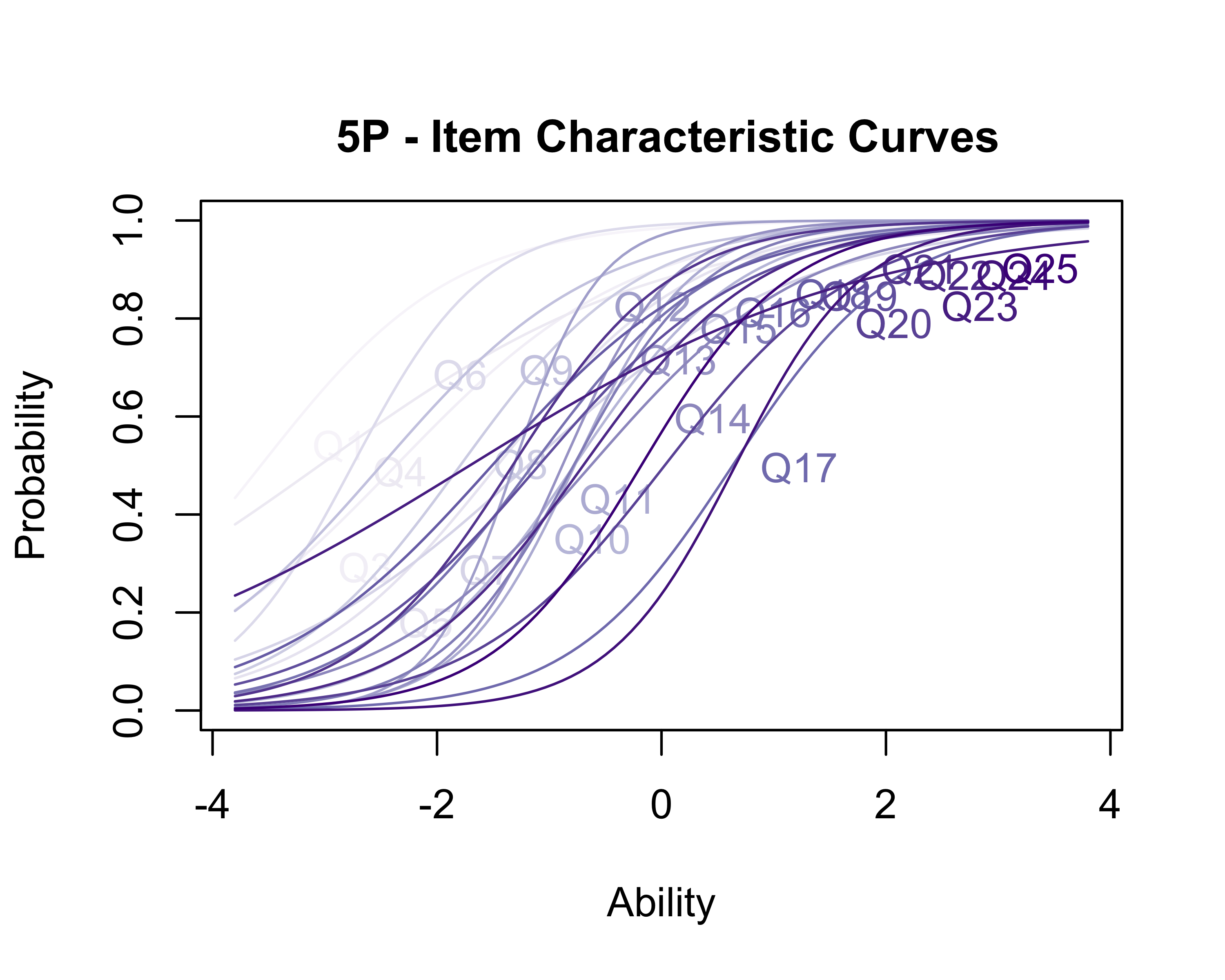
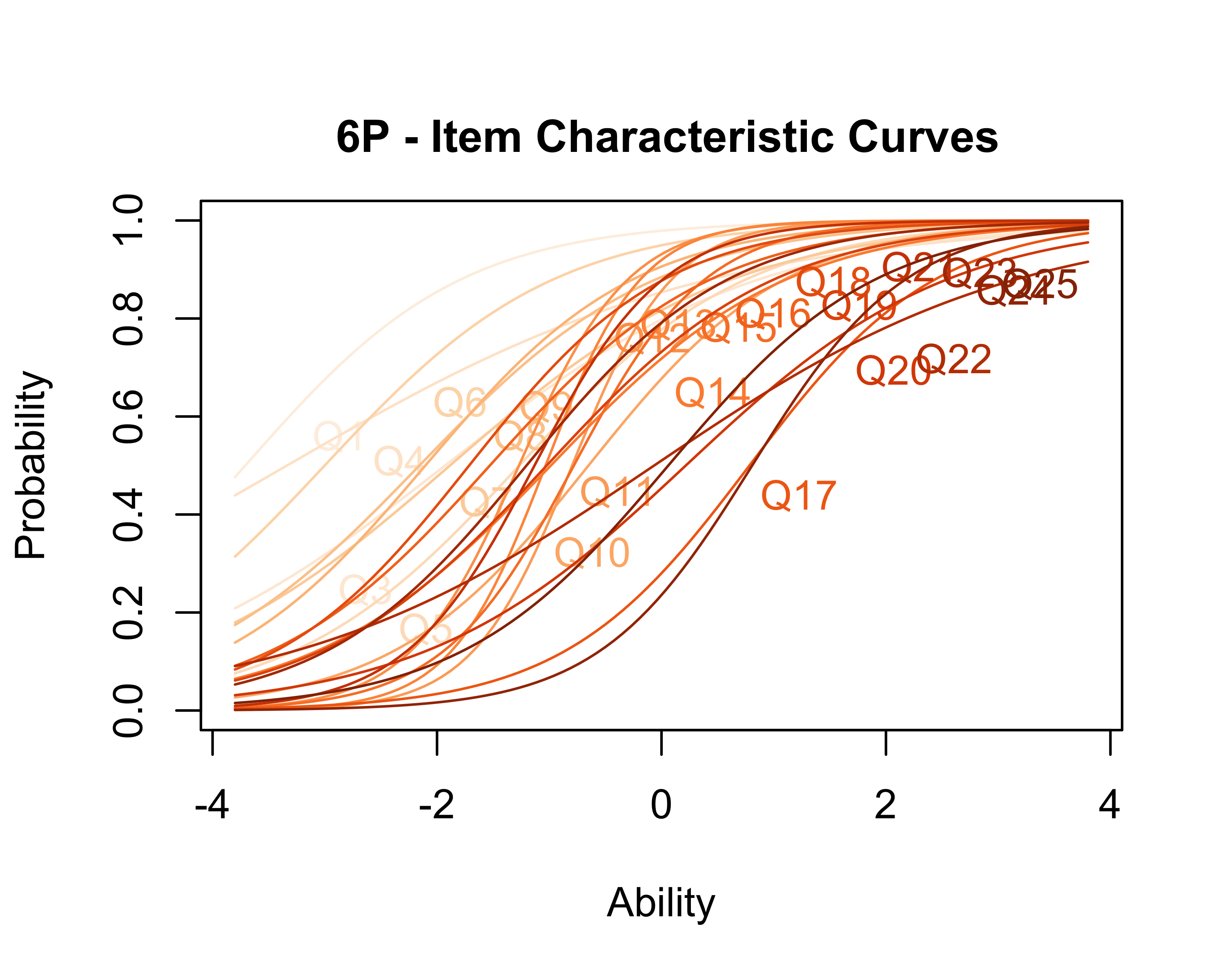
Figure 6: 2-PL IRT Item Characteristic Curves per grade.

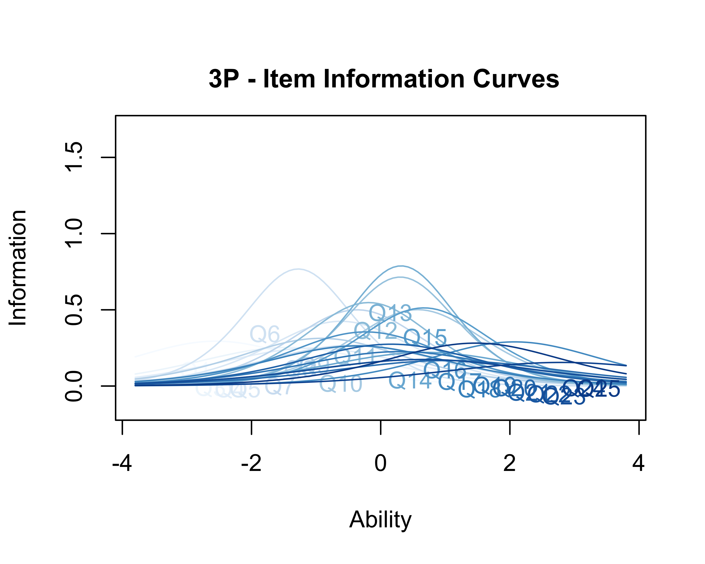
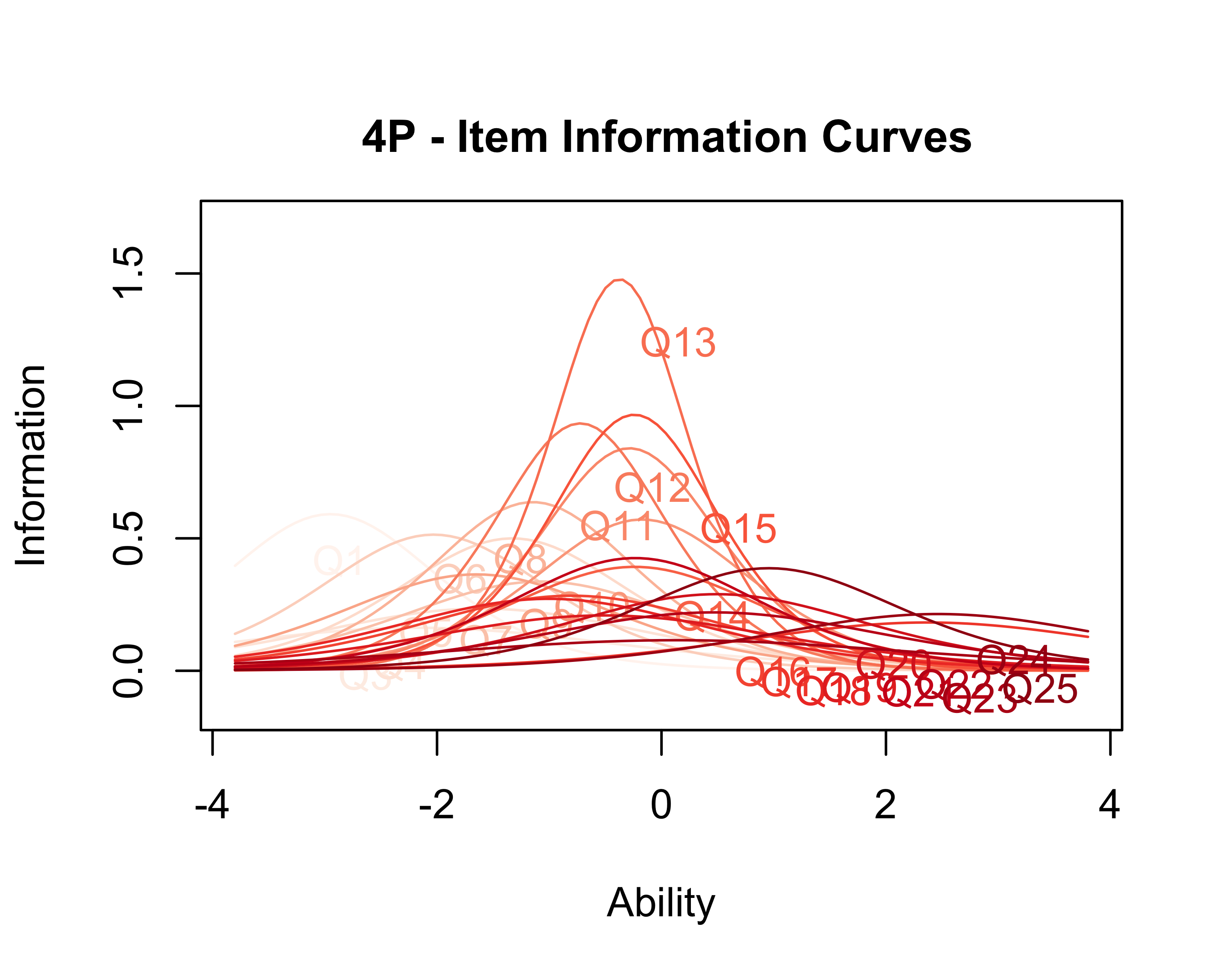
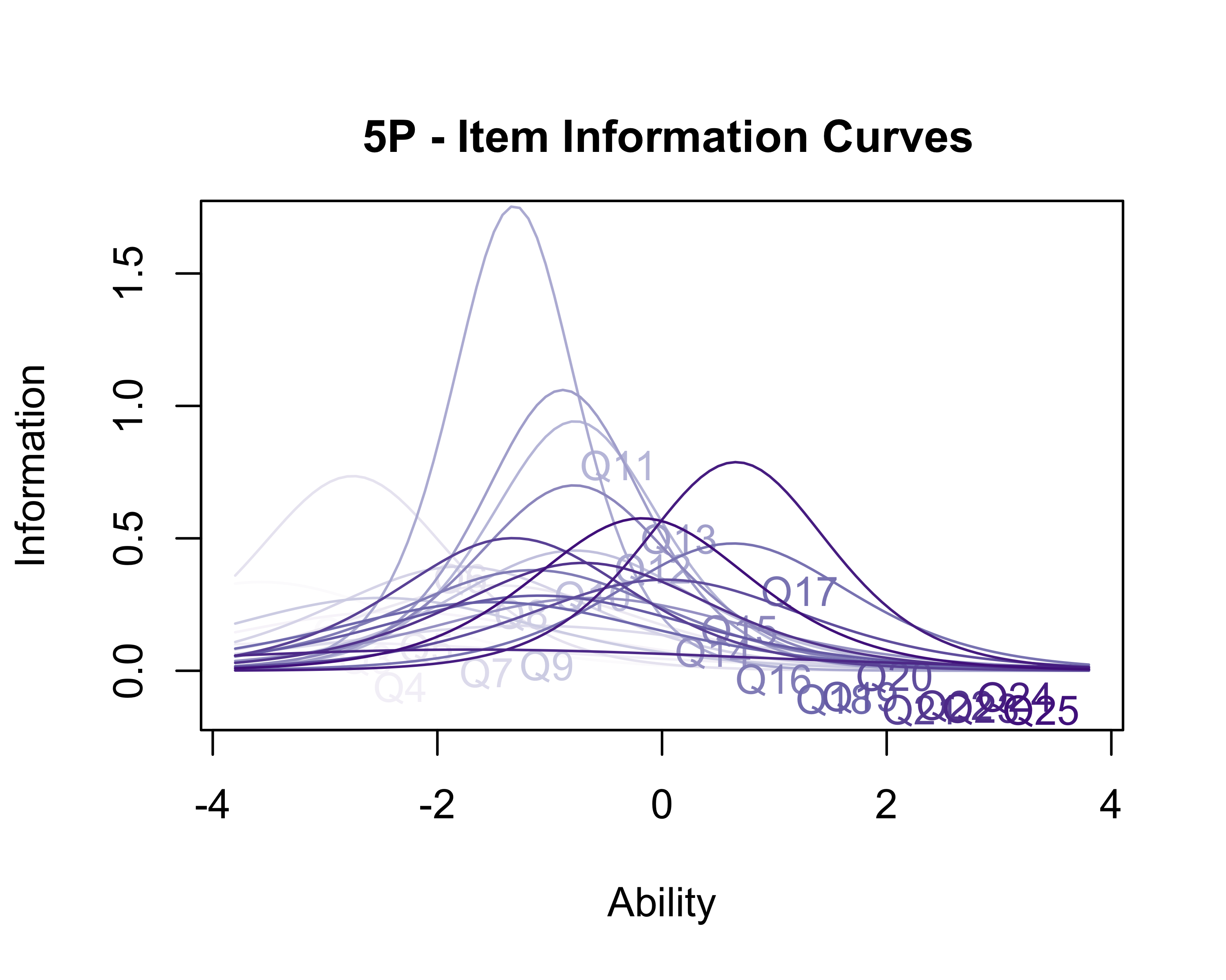
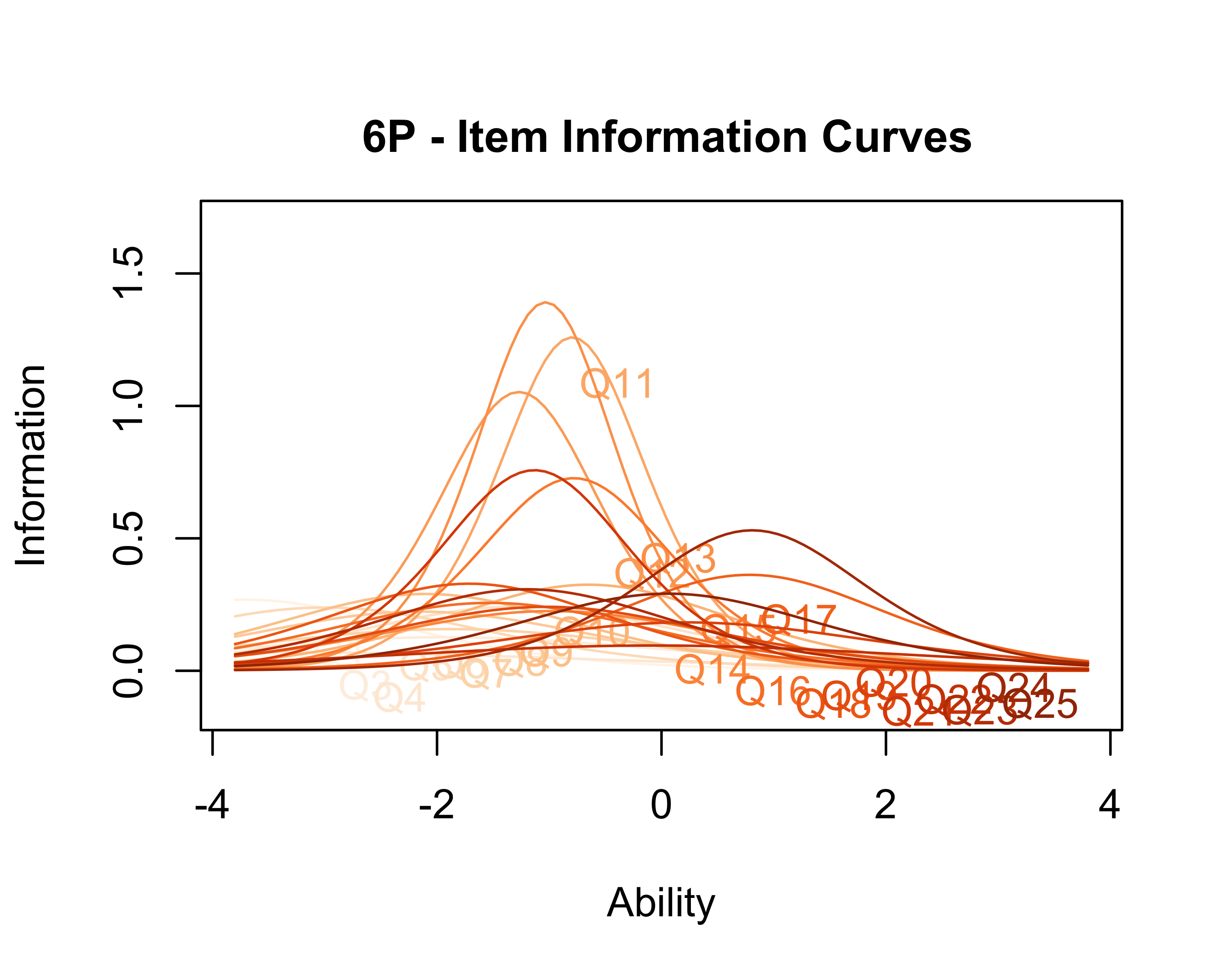
Figure 7: 2-PL IRT Item Information Curves per grade.

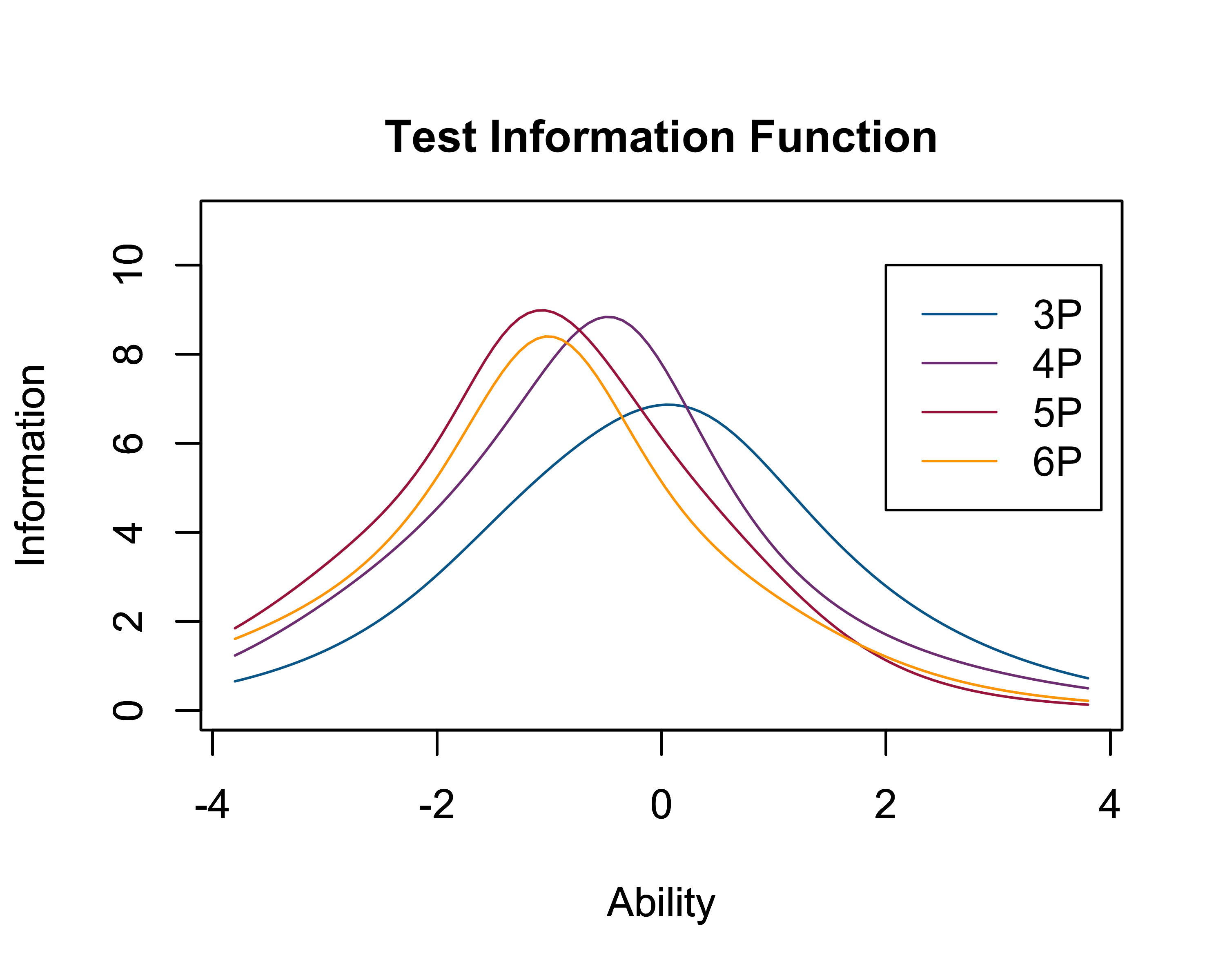
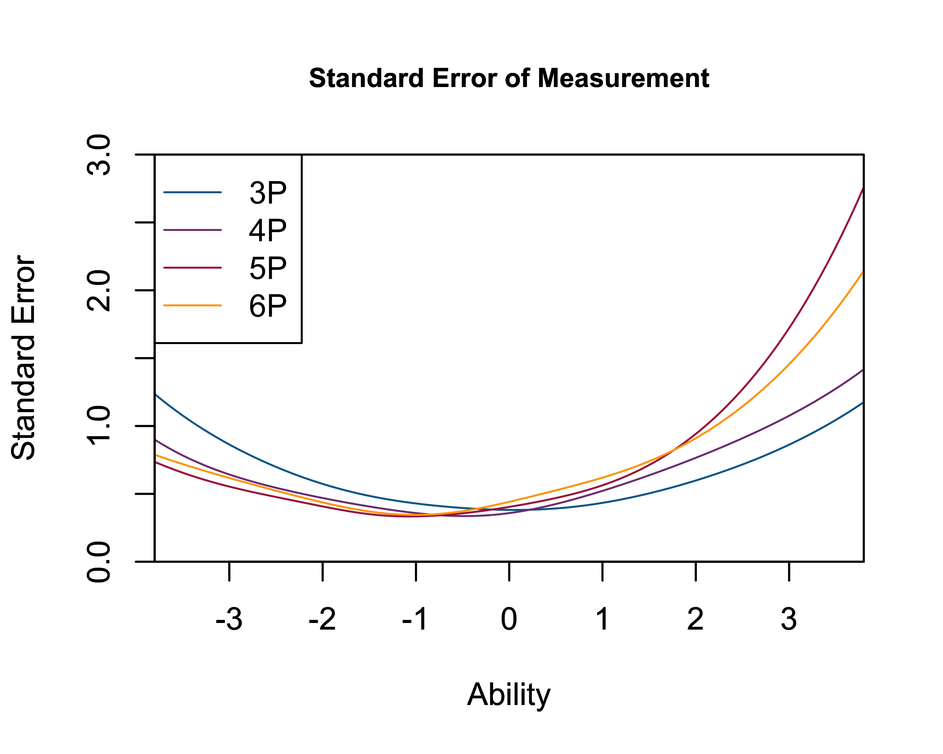
Figure 8: 2-PL IRT Test Information Function (left) and Standard Error of Measurement (right) according to the students’ grade.

A more in depth look into the grade-specific Wright Maps on the 2PL models (see Fig. 9) indicates that for grades 3-4 the items are aligned with the ability of the majority of the candidates, while in grades 5-6 the items are aligned with the ability of a smaller proportion of students, an in particular those who are at the lower end of the logit scale.

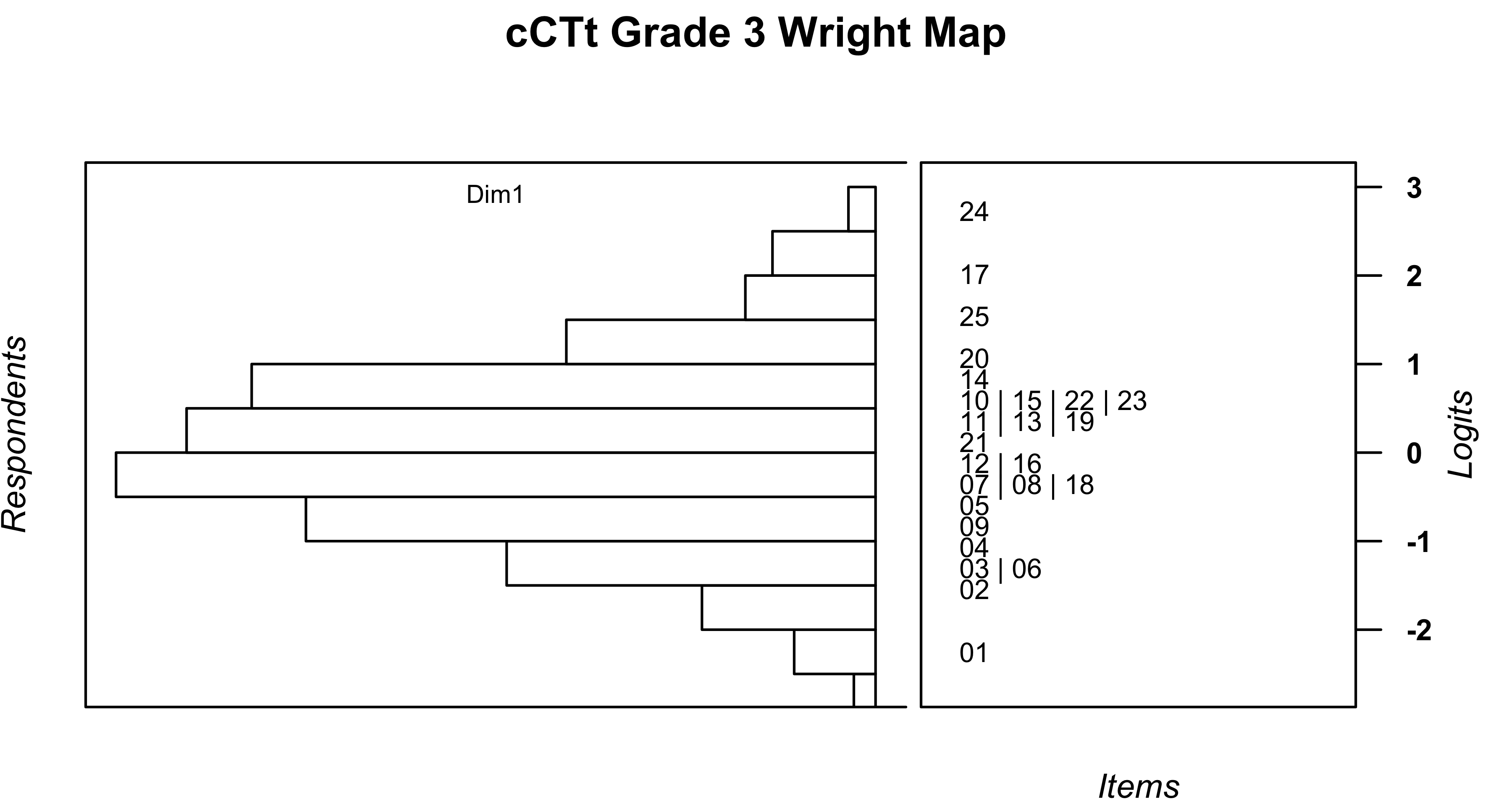
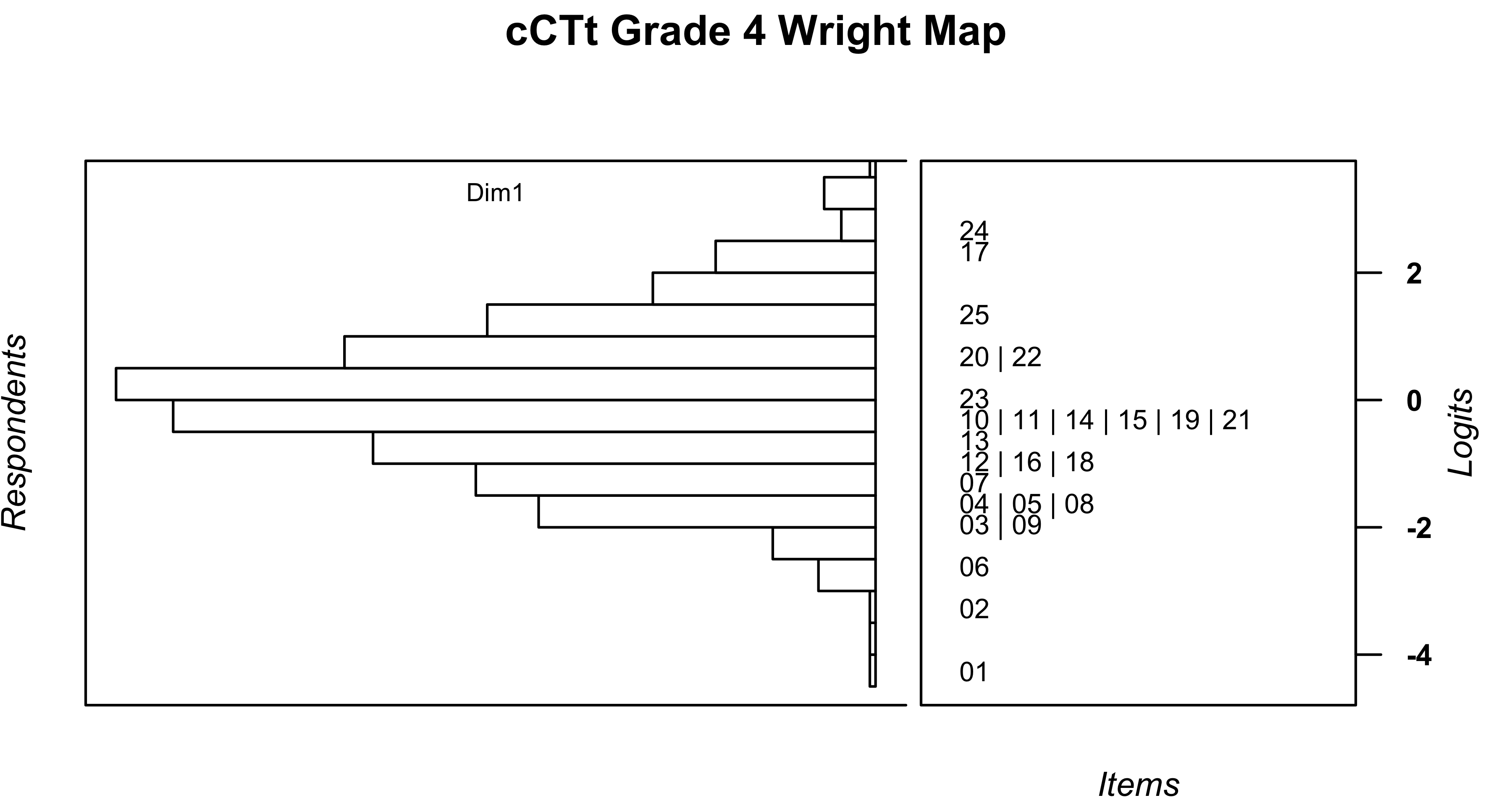
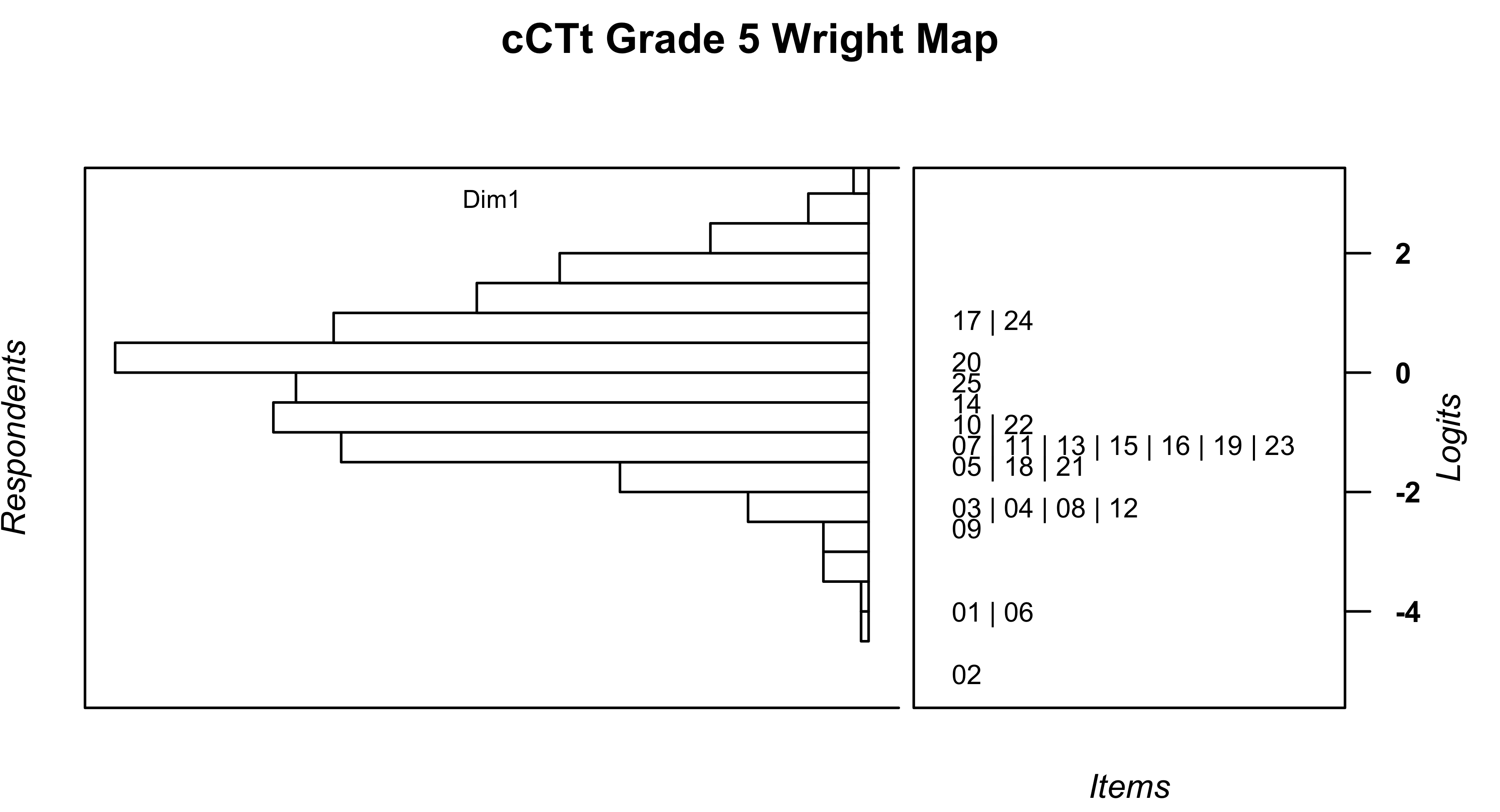
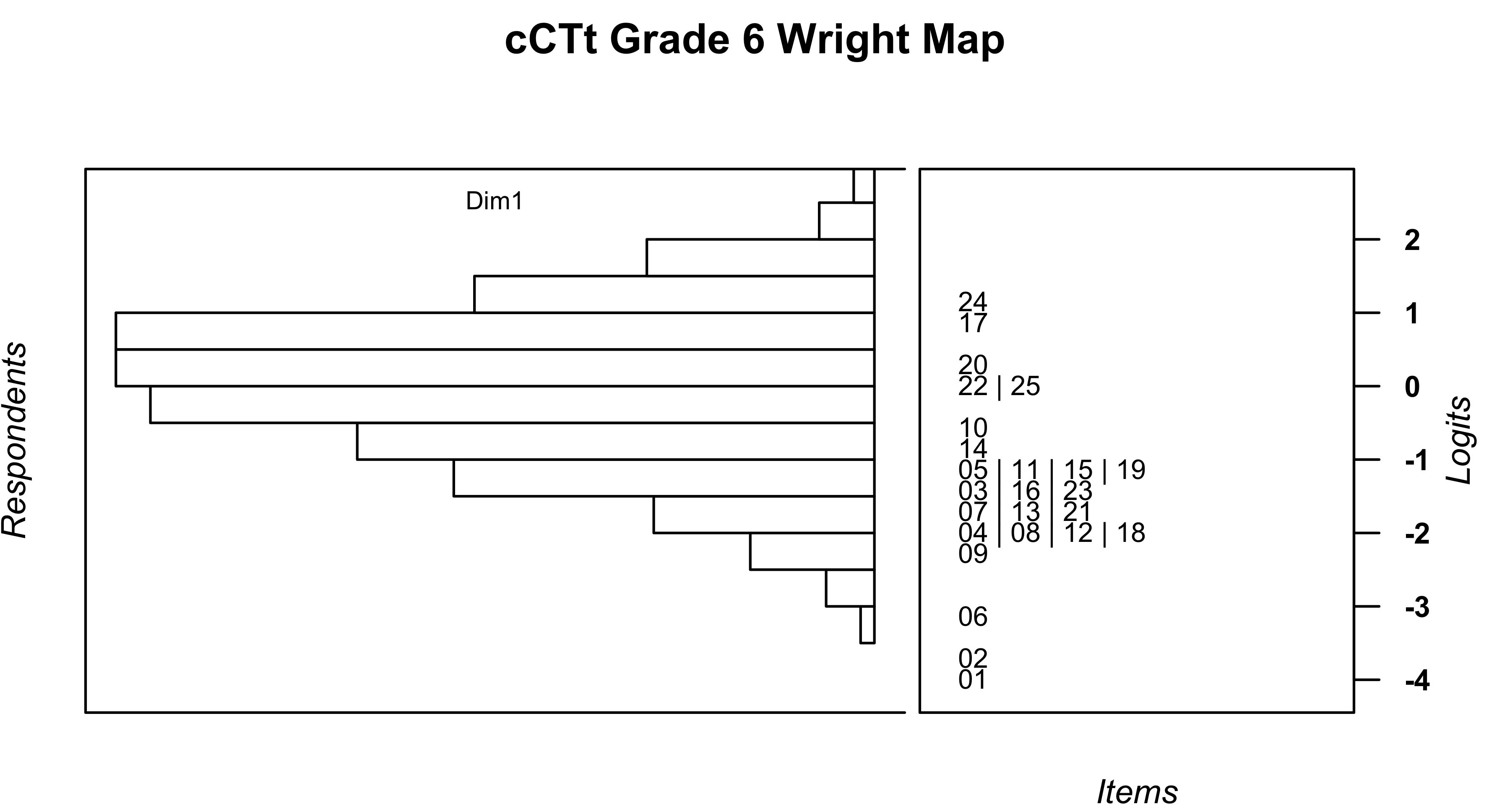
Figure 9: Grade-specific Wright Maps with EAP reliabilities of $0.849$ for grade 3, $0.842$ for grade 4, $0.798$ for grade 5, and $0.78$ for grade 6 and therefore sufficiently high for research purposes.

3.4.5 Proposing Grade-Specific Student Proficiency Profiles

Based on the procedure described by PISA (OECD, 2014, 2017), and the corrected item difficulties provided in Table 12, we establish grade-specific student proficiency profiles with anchor items that are located at the middle of each proficiency level as done by Guggemos et al. (2022). These proficiency profiles with their representative items are described in Table 13.

Table 13: Grade specific proficiency profiles with anchor items (i.e. an item located approximately at the middle of the proficiency level on the logit scale)

	Proficiency level	Logit bounds for the 62% Difficulty values	Items	Types of tasks the students are able to solve for that proficiency level							Percentage of Students
				Sequences	Simple loops	Complex loops	If-else statements	While statements	Combinations of concepts	Not enough items per 0.8 logit to provide a reliable estimate
Grade 3	Level 0	<-1.0	Q1							x	13.1%
	Level 1	[-1.0, -0.2]	Q6, Q3, Q4, Q9, Q5	x	(x)						28.4%
	Level 2	[-0.2, 0.6]	Q8, Q7, Q18, Q12, Q16, Q13, Q11	x	x	x	(x)				33.3%
	Level 3	[0.6, 1.4]	Q21, Q19, Q10, Q15, Q14, Q23, Q22	x	x	x	x	x			18.0%
	Level 4	>1.4	Q20, Q25, Q17, Q24	x	x	x	x	x	x	x	7.2%
Grade 4	Level 0	<-1.7	Q1							x	3.1%
	Level 1	[-1.7, -0.9]	Q6, Q3, Q9, Q4, Q5	x	(x)						14.0%
	Level 2	[-0.9, -0.1]	Q8, Q7, Q18, Q12, Q16, Q13	x	x	x	(x)				26.7%
	Level 3	[-0.1, 0.7]	Q11, Q15, Q19, Q21, Q10, Q14	x	x	x	x				34.8%
	Level 4	[0.7, 1.5]	Q23, Q20, Q22, Q25	x	x	x	x	x	(x)		15.6%
	Level 5	>1.5	Q17, Q24	x	x	x	x	x	x	x	5.7%
Grade 5	Level 0	<-2.5	Q1							x	0.3%
	Level 1	[-2.5, -1.7]	Q6, Q4, Q9, Q3	x							2.6%
	Level 2	[-1.7, -0.9]	Q8, Q12, Q5, Q18, Q21	x	(x)						14.4%
	Level 3	[-0.9, -0.1]	Q23, Q16, Q13, Q19, Q7, Q11, Q15, Q10, Q22, Q14	x	x	x	x	x			26.0%
	Level 4	>-0.1	Q25, Q20, Q24, Q17	x	x	x	x	x	x	x	56.8%
Grade 6	Level 0	<-1.7	Q1, Q6, Q4							x	3.7%
	Level 1	[-1.7, -0.9]	Q9, Q8, Q18, Q7, Q3, Q16, Q12	x	x						13.3%
	Level 2	[-0.9, -0.1]	Q21, Q13, Q5, Q23, Q11, Q19, Q15, Q14, Q10	x	x	x	x	(x)			24.7%
	Level 3	>-0.1	Q25, Q22, Q20, Q24, Q17	x	x	x	x	x	x	x	58.3%

3.4.6 Providing Grade-Agnostic Wright Map and student profiles for longitudinal studies and to establish students’ cognitive maturation according to age

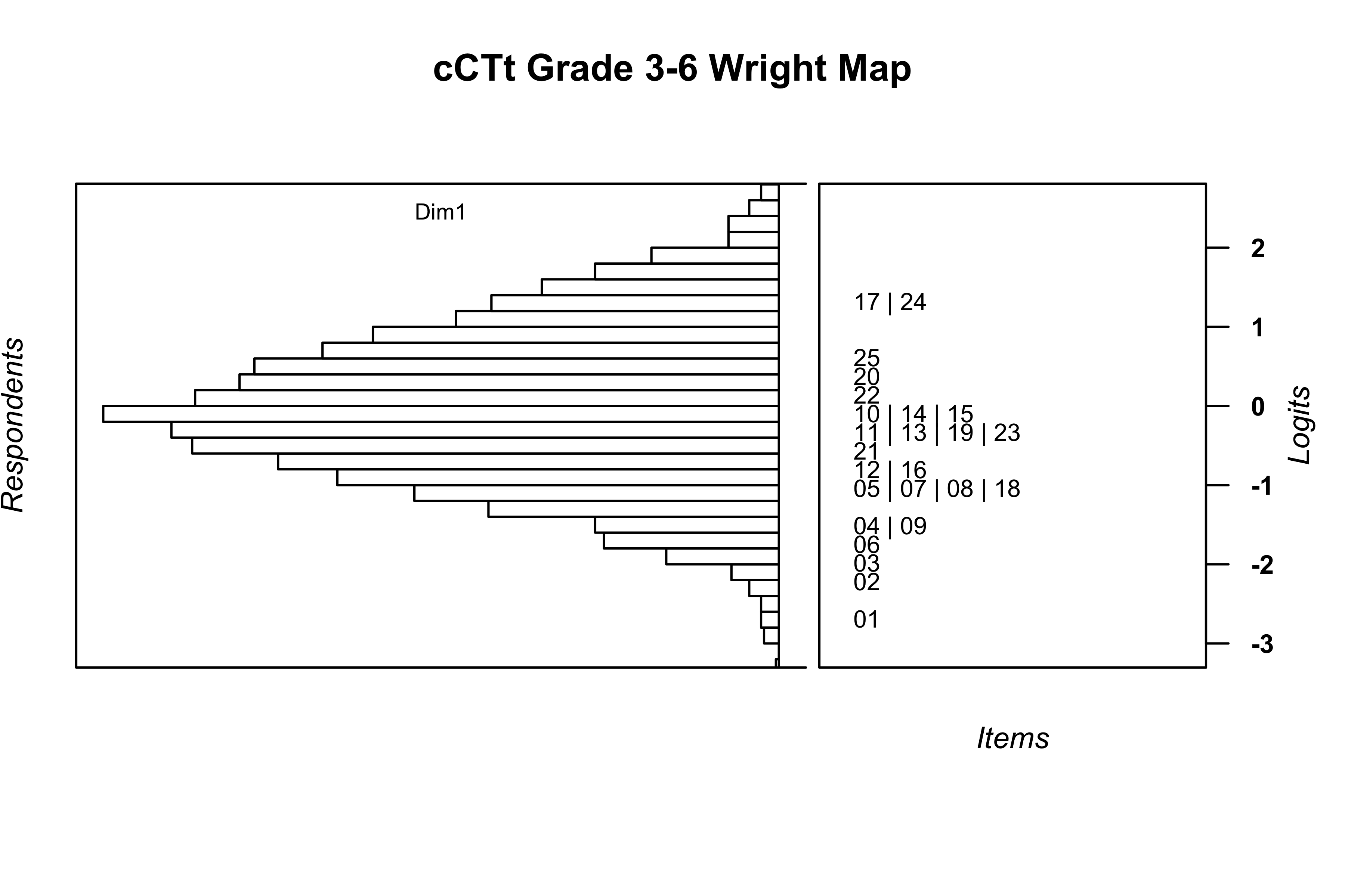
Figure 10: Grade-agnostic cCTt (excluding item Q2) IRT 2PL model Wright Map for all grade 3-6 students

While the grade-specific Wright Maps and student profiles provided are interesting to establish students’ proficiency at a given level, grade-agnostic profiles provide more direct insight into the cognitive maturation of students as they age. To that effect we construct a grade-agnostic 2PL IRT model (see model fit in Table 15, and parameters in Table 16 in appendix A), compute the Wright Map (see Fig. 10 in appendix A), and establish grade-agnostic student proficiency profiles for all students in grades 3-6 (see Table 14). These grade-agnostic profiles can therefore be of use for those interested in evaluating the longitudinal development of students’ CT-concepts. We also indicate in Table 14 the percentage of students per grade at each proficiency level which can provide a baseline for future studies interested in conducting international comparisons (as done by PISA with OECD countries).

Table 14: Grade-agnostic proficiency profiles with anchor items (i.e. an item located approximately at the middle of the proficiency level on the logit scale)

		Level 0	Level 1	Level 2	Level 3	Level 4
Logit bounds for the 62% Difficulty values		<-1.6	[-1.6, -0.8]	[-0.8, 0.0]	[0.0, 0.8]	>0.8
Items		Q1	Q6, Q3, Q4, Q9	Q8, Q5, Q18, Q12, Q7, Q16, Q13, Q21, Q11, Q19	Q15, Q10, Q14, Q23, Q22	Q25, Q20, Q17, Q24
Types of tasks the students are able to solve for that proficiency level	Sequences		x	x	x	x
	Simple loops		(x)	x	x	x
	Complex loops			x	x	x
	If-else statements			x	x	x
	While statements				x	x
	Combinations of concepts					x
	Not enough items per 0.8 logit to provide a reliable estimate	x				x
Percentage of students per proficiency level and grade	Grade 3	8.7%	30.2%	37.4%	17.7%	5.9%
	Grade 4	4.2%	16.7%	32.6%	31.2%	15.5%
	Grade 5	1.0%	6.7%	22.4%	34.0%	35.6%
	Grade 6	1.0%	7.20%	23.4%	36.2%	32.1%

4 Limitations

A number of limitations can be raised concerning this study.

Firstly, the validity of the cCTt for grades 5-6 was compared with data acquired a year prior for a different group of students in grades 3-4. While the measurements took place at the same point of the academic year, there might be certain contextual elements which may impact the students’ results and thus the suitability of the comparison. In particular, the grade 5 students appear to be performing better than the grade 6 students, which is somewhat unexpected (although it may be related to the ceiling effect that we begin to observe in grades 5-6). Indeed other studies have found that students tend to progress on CT-abilities as they get older, without having received any CT-specific instruction (Román-González et al., 2017; Relkin et al., 2020; Relkin and Bers, 2021; Piatti et al., 2022), in alignment with the consideration that Computational Thinking can be considered as a universal skill (Moreno-León et al., 2018). It would thus be interesting to collect data from another subset of students from grades 3-6 at the same point in time and replicate the study.

Secondly, as all the data was collected in a single region, the performance of the students in the sample may differ from that of students in other regions and countries, due to inherent differences in the curricula. It would thus be interesting to expand the validation to students in other countries to determine to what extent the results generalise or are influenced by local curricula. This would also provide the opportunity to conduct Differential Item Functioning across different countries to establish to what extent the cCTt is generalisable (Rachmatullah et al., 2022).

Finally, the IRT analysis employed the same model for all grades (2-PL) in order to facilitate their comparison, although the 3-PL model may have been better suited for certain grades. Furthermore, there was a small mis-specification of the unidimensionality criteria. It thus remains likely that the discrimination parameters were slightly overestimated.

More generally, paper-based assessments, such as the cCTt and those presented in the literature review, should be considered within a systems of assessments (Grover et al., 2015; Román-González et al., 2019; Guggemos et al., 2022) to gain a more comprehensive picture of students’ CT competence. This is because paper-based assessments tend to lack insight into CT-processes (generally acquired through educational data mining) and CT-perspectives (generally acquired through self-assessment scales such as the Computational Thinking Scale by Korkmaz et al. (2017) as was done by Guggemos et al. 2022), with few studies having also looked into the link between CT and other abilities (such as numerical, verbal reasoning, and non verbal visuo-spatial abilities as was done by  Tsai et al. (2022) or spatial, reasoning, and problem solving abilities as was done by Román-González et al. 2017).

5 Conclusion

Assessments that are useful to researchers, educators and practitioners, may be used in longitudinal studies, and provide the means of transitioning between assessments (e.g. through equivalency scales), are particularly relevant in K-12 to understand the impact of the ever increasing Computer Science and Computational Thinking initiatives in formal education.

In the present context we were interested in addressing this issue in the case of primary school with the competent CT test, a derivative of the Beginners’ CT test by Zapata-Cáceres et al. (2020) and the parent CT test by Román-González et al. (2017). This study therefore looked to expand on the validation of the cCTt to determine whether it could be employed in multi-year longitudinal studies between grades 3 and 6 (ages 7-11), provide student proficiency profiles, and determine at which point a transition to the CT test should be envisioned and how. While the parent CTt, which was validated for students in grades 5-10, may have been envisioned to continue to monitor students’ progress, no equivalency scale exists yet between these two instruments, nor, to the best of our knowledge, between any other CT instruments. Therefore, using i) data from the administration of the cCTt between November 2021 and January 2022 to 1209 grade 5-6 students (585 in grade 5, 624 in grade 6) and ii) and data acquired from the administration of the cCTt in January 2021 (El-Hamamsy et al., 2022c) to 1457 grade 3-4 students (709 in grade 3, 748 in grade 4), the present study assessed the psychometric properties of the cCTt in grades 5-6 and compared them with grades 3-4 to establish the limits of validity of the cCTt for these age groups. The psychometric analysis considered conjointly the results of Classical Test Theory, Item Response Theory, and Differential Item Functioning to evaluate the properties of the cCTt for students in grades 3-6.

Validity and reliability of the cCTt in grades 3-6 and the link with cognitive and developmental maturation.

The results from the psychometric analysis confirm that the cCTt is valid and reliable for students in grades 3-6 and provides distinct proficiency profiles that describe the “computational thinking tasks that students on a specific level are systematically able to master but which cannot be mastered by students on a lower level” (Guggemos et al., 2022). Nonetheless, a ceiling effect starts to appear in grades 5-6 as the students perform well on the easier CT-concepts pertaining to sequences and loops. It would therefore be interesting to propose items pertaining to more advanced concepts to improve the reliability of the instrument for grades 5-6. Furthermore, the significant difference in scores across grades further stresses the importance of having targeted grade specific instruments to improve the validity and reliability of proposed assessments. As the BCTt validation (Zapata-Cáceres et al., 2020), the BCTt - cCTt comparison (El-Hamamsy et al., 2022d), and development of the TechCheck and its variants (Relkin et al., 2020; Relkin and Bers, 2021; Relkin, 2022) showed, it is difficult to have a single assessment which is valid and reliable for a broad age range in primary school. This is unsurprising given the rapid cognitive development students undergo at this time of their lives. Indeed, as stated by El-Hamamsy et al. (2022d), CT is correlated with other cognitive abilities (e.g. numerical, verbal, non-verbal) (Tsarava et al., 2022) that are related to students’ maturation, increase in working memory Gathercole et al., 2004; Cowan, 2016, and executive functions (Arfé et al., 2019; Robertson et al., 2020; Robledo-Castro et al., 2023), thus improving their capacity to solve complex computational problems. As such, it is both unsurprising to see significant improvements over time, and difficult to have a single instrument that can be reliably employed in multi-year longitudinal studies. Indeed, a corollary finding from the present analysis is that students, as they get older, have a good mastery of easier CT-concepts, but appear to still have a possible margin of progression for more advanced concepts such as conditional statements, while statements and in particular their combination. Indeed, it would appear that grade 5-6 students require targeted instruction to progress on these more advanced CT-concepts, thus providing insight for interventions in this age group. From a cognitive development perspective, it therefore appears that certain CT-concepts are easier than others, which helps derive a developmental progression from sequences, to loops, to conditionals and while statements. The findings from the study, and in particular the student profiles established, can therefore contribute to further tailoring CT assessments for the successive stages of their cognitive development.

The importance of providing means of transitioning between instruments across grades, including between the cCTt and CTt in grades 5-6.

Given that the findings established the relevance of developing more grade specific instruments across primary school, it is all the more critical for researchers and practitioners to have means of seamlessly transitioning between instruments of a given assessment family. Therefore, provided the validity of both instruments in grades 5-6, the findings confirm that grades 5-6 is an interesting point to transition between the cCTt and the CTt. Therefore, future work should consider comparing the cCTt and the CTt in grades 5-6, as was done for BCTt and cCTt for grades 3-4 in El-Hamamsy et al. (2022d). Such a comparison should be performed with a comparable group of students in order to establish equivalency scales which would help assess students’ CT development in the long run. These equivalency scales can be achieved using Z-scoring (and percentiles) as was done here and in other studies (Román-González et al., 2017; Relkin, 2022), as it provides normalised cCTt scores across grades which makes it possible to compare between grades. We argue that such percentiles should be grade-specific (without aggregating students in several grades), and established using comparable populations (i.e. from similar educational systems) both intra- and inter-assessments in order to provide a reliable means of comparing results across grades and passing from one instrument to another.

The importance of gender-fairness analyses in the CT literature.

Finally, the present study contributes to the literature by guaranteeing that the cCTt is a fair assessment with respect to gender through gender Differential Item Functioning. Given the present scarcity of such types of analyses in the CT assessment literature, we propose that gender Differential Item Functioning should become more standard practice in CT assessment validations to ensure that the proposed instruments are of relevance to the educator and research communities, particularly for those looking to address gender gaps in computing.

To conclude, in addition to validating and providing recommendations for the use of the cCTt in grades 3-6 (ages 7-11), the findings contribute to improving the design of longitudinal research on the acquisition of CT-concepts. In combination with insight into cognitive process at play (e.g. CT-practices such as abstraction, algorithmic thinking, decomposition, evaluation and generalisation, Selby and Woollard, 2013) and in accordance with the theory of constructive alignment (Biggs, 1996), it should be possible to provide guidelines for the design of developmentally appropriate learning objectives, assessments, and interventions for each level of primary school that account for both the type of cognitive processes and concepts that students are able to engage with at a given age.

Data availability

The data will be publicly available on Zenodo upon publication (doi: 10.5281/zenodo.7983525, El-Hamamsy et al., 2023).

Ethics

The researchers were granted ethical approval to conduct the study by the head of the Department of Education and by the Human Research Ethics Committee of EPFL (project HREC 033-2019). Teachers were provided an explanation of the research objectives during the first training session. They were then informed of their rights and in particular that they could i) opt out of the research and any data collection at any point in time and ii) could request that any data collected be deleted.

Conflicts of Interest

The authors declare that there were no conflicts of interest involved with the realisation of the present study.

Appendix A Grade-agnostic IRT Model and Wright map

Table 15: Grade-agnostic cCTt (excluding item Q2) IRT Model comparison using ANOVA

Grade	Model	AIC	BIC	Log Likelihood	LRT	df	p-value
All	1PL	62377.34	62524.58	-31163.67
	2PL	61891.00	62173.69	-30897.50	532.34	23	$<0.001$

Table 16: Grade-agnostic cCTt (excluding item Q2) IRT 2PL Model Parameters

	Dffclt	Dscrmn	Dffclt 62%
Q1	-2.913	1.279	-2.530
Q3	-2.036	0.808	-1.430
Q4	-1.707	0.926	-1.178
Q5	-1.175	1.154	-0.750
Q6	-1.896	1.607	-1.592
Q7	-1.033	0.994	-0.540
Q8	-1.079	1.521	-0.758
Q9	-1.514	1.284	-1.132
Q10	-0.182	1.529	0.138
Q11	-0.339	2.078	-0.104
Q12	-0.779	2.139	-0.550
Q13	-0.420	2.400	-0.216
Q14	-0.223	1.220	0.178
Q15	-0.232	1.960	0.017
Q16	-0.801	1.236	-0.405
Q17	1.263	1.267	1.650
Q18	-0.980	1.201	-0.572
Q19	-0.477	1.127	-0.043
Q20	0.422	1.007	0.908
Q21	-0.524	1.538	-0.205
Q22	0.097	0.978	0.597
Q23	-0.303	1.001	0.186
Q24	1.357	1.317	1.728
Q25	0.520	1.429	0.862
M	-0.623	1.375	-0.239
SD	0.997	0.413	0.985
Min	-2.913	0.808	-2.530
25%	-1.103	1.097	-0.752
50%	-0.500	1.273	-0.211
75%	-0.213	1.531	0.180
MAX	1.357	2.400	1.728

References

- Alavi et al. (2020) Alavi, M., Visentin, D. C., Thapa, D. K., Hunt, G. E., Watson, R., and Cleary, M. (2020). Chi-square for model fit in confirmatory factor analysis. Journal of Advanced Nursing, 76(9):2209–2211.
- Araujo et al. (2017) Araujo, A. L. S. O., Santos, J. S., Andrade, W. L., Guerrero, D. D. S., and Dagienė, V. (2017). Exploring computational thinking assessment in introductory programming courses. In 2017 IEEE Frontiers in Education Conference (FIE), pages 1–9.
- Arfé et al. (2019) Arfé, B., Vardanega, T., Montuori, C., and Lavanga, M. (2019). Coding in Primary Grades Boosts Children’s Executive Functions. Frontiers in Psychology, 10.
- Baker (2001) Baker, F. B. (2001). The basics of item response theory. ERIC Clearinghouse on Assessment and Evaluation, College Park, Md., 2nd ed edition.
- Bean and Bowen (2021) Bean, G. J. and Bowen, N. K. (2021). Item Response Theory and Confirmatory Factor Analysis: Complementary Approaches for Scale Development. Journal of Evidence-Based Social Work, 18(6):597–618.
- Bellettini et al. (2015) Bellettini, C., Lonati, V., Malchiodi, D., Monga, M., Morpurgo, A., and Torelli, M. (2015). How Challenging are Bebras Tasks? An IRT Analysis Based on the Performance of Italian Students. In Proceedings of the 2015 ACM Conference on Innovation and Technology in Computer Science Education, ITiCSE ’15, pages 27–32, New York, NY, USA. Association for Computing Machinery.
- Bers et al. (2022) Bers, M. U., Strawhacker, A., and Sullivan, A. (2022). The state of the field of computational thinking in early childhood education. OECD Education Working Papers 274.
- Biggs (1996) Biggs, J. (1996). Enhancing teaching through constructive alignment. Higher education, 32(3):347–364.
- Bland and Altman (1997) Bland, J. M. and Altman, D. G. (1997). Statistics notes: Cronbach’s alpha. Bmj, 314(7080):572.
- Brennan and Resnick (2012) Brennan, K. and Resnick, M. (2012). New frameworks for studying and assessing the development of computational thinking. page 25.
- Chae et al. (2019) Chae, Y.-m., Park, S. G., and Park, I. (2019). The relationship between classical item characteristics and item response time on computer-based testing. Korean J Med Educ, 31(1):1–9.
- Chen et al. (2017) Chen, G., Shen, J., Barth-Cohen, L., Jiang, S., Huang, X., and Eltoukhy, M. (2017). Assessing elementary students’ computational thinking in everyday reasoning and robotics programming. Comput Educ, 109:162–175.
- Christensen et al. (2017) Christensen, K. B., Makransky, G., and Horton, M. (2017). Critical Values for Yen’s Q : Identification of Local Dependence in the Rasch Model Using Residual Correlations. Applied Psychological Measurement, 41(3):178–194.
- Commission et al. (2022) Commission, E., Centre, J. R., Bocconi, S., Chioccariello, A., Kampylis, P., Dagienė, V., Wastiau, P., Engelhardt, K., Earp, K., Horvath, M., Jasutė, M., Malagoli, C., Masiulionytė-Dagienė, V., Stupurienė, G., and Giannoutsou, N. (2022). Reviewing computational thinking in compulsory education : state of play and practices from computing education.
- Cowan (2016) Cowan, N. (2016). Working Memory Maturation: Can We Get at the Essence of Cognitive Growth? Perspect Psychol Sci, 11(2):239–264. Publisher: SAGE Publications Inc.
- Cutumisu et al. (2019) Cutumisu, M., Adams, C., and Lu, C. (2019). A Scoping Review of Empirical Research on Recent Computational Thinking Assessments. J Sci Educ Technol, 28(6):651–676.
- Dai et al. (2020) Dai, B., Zhang, W., Wang, Y., and Jian, X. (2020). Comparison of Trust Assessment Scales Based on Item Response Theory. Frontiers in Psychology, 11:10.
- Dai et al. (2022) Dai, S., Wang, X., and Svetina, D. (2022). subscore: Computing Subscores in Classical Test Theory and Item Response Theory. R package version 3.3.
- De Ayala and Little (2022) De Ayala, R. J. and Little, T. D. (2022). The theory and practice of item response theory. Methodology in the social sciences. The Guilford Press, New York, second edition.
- De Champlain (2010) De Champlain, A. F. (2010). A primer on classical test theory and item response theory for assessments in medical education. Medical Education, 44(1):109–117. _eprint: https://onlinelibrary.wiley.com/doi/pdf/10.1111/j.1365-2923.2009.03425.x.
- del Olmo-Muñoz et al. (2020) del Olmo-Muñoz, J., Cózar-Gutiérrez, R., and González-Calero, J. A. (2020). Computational thinking through unplugged activities in early years of Primary Education. Comput Educ, 150:103832.
- DeVellis (2006) DeVellis, R. F. (2006). Classical Test Theory. Medical Care, 44(11):S50–S59.
- El-Hamamsy et al. (2023) El-Hamamsy, L., , Zufferey, B. B. J. D., and Mondada, F. (2023). Extended dataset for the validation the competent Computational Thinking test in grades 3-6.
- El-Hamamsy et al. (2022a) El-Hamamsy, L., Bruno, B., Avry, S., Chessel-Lazzarotto, F., Zufferey, J. D., and Mondada, F. (2022a). The tacs model: Understanding primary school teachers’ adoption of computer science pedagogical content. ACM Trans. Comput. Educ.
- El-Hamamsy et al. (2021) El-Hamamsy, L., Chessel-Lazzarotto, F., Bruno, B., Roy, D., Cahlikova, T., Chevalier, M., Parriaux, G., Pellet, J.-P., Lanarès, J., Zufferey, J. D., and Mondada, F. (2021). A computer science and robotics integration model for primary school: evaluation of a large-scale in-service K-4 teacher-training program. Education and Information Technologies, 26(3):2445–2475.
- El-Hamamsy et al. (2022b) El-Hamamsy, L., Zapata-Cáceres, M., Barroso, E. M., Mondada, F., Zufferey, J. D., and Bruno, B. (2022b). The competent computational thinking test: Development and validation of an unplugged computational thinking test for upper primary school. Journal of Educational Computing Research, page 07356331221081753.
- El-Hamamsy et al. (2022c) El-Hamamsy, L., Zapata-Cáceres, M., Barroso, E. M., Mondada, F., Zufferey, J. D., and Bruno, B. (2022c). Dataset for the validation of a Computational Thinking test for upper primary school (grades 3-4).
- El-Hamamsy et al. (2022d) El-Hamamsy, L., Zapata-Cáceres, M., Marcelino, P., Dehler Zufferey, J., Bruno, B., Martín-Barroso, E., and Román-González, M. (2022d). Comparing the psychometric properties of two primary school computational thinking (ct) assessments for grades 3 and 4: the beginners’ ct test (bctt) and the competent ct test (cctt). Frontiers in Psychology.
- Gane et al. (2021) Gane, B. D., Israel, M., Elagha, N., Yan, W., Luo, F., and Pellegrino, J. W. (2021). Design and validation of learning trajectory-based assessments for computational thinking in upper elementary grades. Computer Science Education, 31(2):141–168.
- Gathercole et al. (2004) Gathercole, S. E., Pickering, S. J., Ambridge, B., and Wearing, H. (2004). The Structure of Working Memory From 4 to 15 Years of Age. Developmental Psychology, 40:177–190. Place: US Publisher: American Psychological Association.
- Gravetter et al. (2020) Gravetter, F. J., Wallnau, L. B., Forzano, L.-A. B., and Witnauer, J. E. (2020). Essentials of statistics for the behavioral sciences. Cengage Learning.
- Grover et al. (2015) Grover, S., Pea, R., and Cooper, S. (2015). Systems of assessments” for deeper learning of computational thinking in k-12. In Proceedings of the 2015 annual meeting of the American educational research association, pages 15–20.
- Guggemos et al. (2022) Guggemos, J., Seufert, S., and Román-González, M. (2022). Computational Thinking Assessment – Towards More Vivid Interpretations. Tech Know Learn.
- Hambleton and Jones (1993) Hambleton, R. K. and Jones, R. W. (1993). Comparison of classical test theory and item response theory and their applications to test development. Educational measurement: issues and practice, 12(3):38–47.
- Hambleton et al. (1991) Hambleton, R. K., Swaminathan, H., and Rogers, H. J. (1991). Fundamentals of Item Response Theory. SAGE. Google-Books-ID: gW05DQAAQBAJ.
- Hinton et al. (2014) Hinton, P., McMurray, I., and Brownlow, C. (2014). SPSS explained. Routledge.
- Hsu et al. (2018) Hsu, T.-C., Chang, S.-C., and Hung, Y.-T. (2018). How to learn and how to teach computational thinking: Suggestions based on a review of the literature. Comput Educ, 126:296–310.
- Hu and Bentler (1999) Hu, L.-t. and Bentler, P. M. (1999). Cutoff criteria for fit indexes in covariance structure analysis: Conventional criteria versus new alternatives. Structural Equation Modeling: A Multidisciplinary Journal, 6(1):1–55.
- Hubwieser and Mühling (2014) Hubwieser, P. and Mühling, A. (2014). Playing PISA with bebras. In Proceedings of the 9th Workshop in Primary and Secondary Computing Education, WiPSCE ’14, pages 128–129, New York, NY, USA. Association for Computing Machinery.
- Irribarra and Freund (2014) Irribarra, D. T. and Freund, R. (2014). Wright Map: IRT item-person map with ConQuest integration.
- Jabrayilov et al. (2016) Jabrayilov, R., Emons, W. H. M., and Sijtsma, K. (2016). Comparison of Classical Test Theory and Item Response Theory in Individual Change Assessment. Appl Psychol Meas, 40(8):559–572.
- Kahraman (2013) Kahraman, N. (2013). Unidimensional Interpretations for Multidimensional Test Items. Journal of Educational Measurement, 50(2):227–246.
- Kong and Lai (2022) Kong, S.-C. and Lai, M. (2022). Validating a computational thinking concepts test for primary education using item response theory: An analysis of students’ responses. Computers & Education, 187:104562.
- Korkmaz et al. (2017) Korkmaz, O., Cakir, R., and Ozden, M. Y. (2017). A validity and reliability study of the computational thinking scales (CTS). Computers in Human Behavior, 72:558–569.
- Kyriazos (2018) Kyriazos, T. A. (2018). Applied Psychometrics: Writing-Up a Factor Analysis Construct Validation Study with Examples. Psychology, 9(11):2503–2530.
- Li et al. (2021) Li, Y., Xu, S., and Liu, J. (2021). Development and Validation of Computational Thinking Assessment of Chinese Elementary School Students. Journal of Pacific Rim Psychology, 15.
- Magis et al. (2020) Magis, D., Beland, S., Raiche, G., and Magis, M. D. (2020). Package ‘difr’.
- Magis et al. (2010) Magis, D., Beland, S., Tuerlinckx, F., and De Boeck, P. (2010). A general framework and an r package for the detection of dichotomous differential item functioning. Behavior Research Methods, 42:847–862.
- Magis et al. (2011) Magis, D., Raîche, G., Béland, S., and Gérard, P. (2011). A Generalized Logistic Regression Procedure to Detect Differential Item Functioning Among Multiple Groups. International Journal of Testing, 11(4):365–386.
- Marinus et al. (2018) Marinus, E., Powell, Z., Thornton, R., McArthur, G., and Crain, S. (2018). Unravelling the Cognition of Coding in 3-to-6-year Olds: The development of an assessment tool and the relation between coding ability and cognitive compiling of syntax in natural language. In Proceedings of the 2018 ACM Conference on International Computing Education Research, pages 133–141, Espoo Finland. ACM.
- Master et al. (2021) Master, A., Meltzoff, A. N., and Cheryan, S. (2021). Gender stereotypes about interests start early and cause gender disparities in computer science and engineering. PNAS, 118(48).
- Moreno-León et al. (2018) Moreno-León, J., Román-González, M., and Robles, G. (2018). On computational thinking as a universal skill: A review of the latest research on this ability. In 2018 IEEE Global Engineering Education Conference (EDUCON), pages 1684–1689.
- Mouza et al. (2020) Mouza, C., Pan, Y.-C., Yang, H., and Pollock, L. (2020). A Multiyear Investigation of Student Computational Thinking Concepts, Practices, and Perspectives in an After-School Computing Program. Journal of Educational Computing Research, 58(5):1029–1056. Publisher: SAGE Publications Inc.
- O. A. and E. R. I. (2016) O. A., A. and E. R. I., A. (2016). Comparative Analysis of Classical Test Theory and Item Response Theory Based Item Parameter Estimates of Senior School Certificate Mathematics Examination. ESJ, 12(28):263.
- OECD (2014) OECD (2014). PISA 2012 Technical Report. Technical report, OECD Publishing.
- OECD (2017) OECD (2017). PISA 2015 Technical Report. Technical report, OECD Publishing.
- Parker et al. (2021) Parker, M. C., Kao, Y. S., Saito-Stehberger, D., Franklin, D., Krause, S., Richardson, D., and Warschauer, M. (2021). Development and preliminary validation of the assessment of computing for elementary students (aces). In Proc. 52nd ACM Tech. Symp. Comput. Sci. Educ., SIGCSE ’21, page 10–16, New York, NY, USA. Association for Computing Machinery.
- Pellegrino et al. (2016) Pellegrino, J. W., DiBello, L. V., and Goldman, S. R. (2016). A Framework for Conceptualizing and Evaluating the Validity of Instructionally Relevant Assessments. Educational Psychologist, 51(1):59–81. Publisher: Routledge _eprint: https://doi.org/10.1080/00461520.2016.1145550.
- Piatti et al. (2022) Piatti, A., Adorni, G., El-Hamamsy, L., Negrini, L., Assaf, D., Gambardella, L., and Mondada, F. (2022). The CT-cube: A framework for the design and the assessment of computational thinking activities. Computers in Human Behavior Reports, page 100166.
- Prudon (2015) Prudon, P. (2015). Confirmatory Factor Analysis as a Tool in Research Using Questionnaires: A Critique,. Comprehensive Psychology, 4:03.CP.4.10.
- R Core Team (2019) R Core Team (2019). R: A Language and Environment for Statistical Computing. R Foundation for Statistical Computing, Vienna, Austria.
- Rachmatullah et al. (2022) Rachmatullah, A., Vandenberg, J., and Wiebe, E. (2022). Toward More Generalizable CS and CT Instruments: Examining the Interaction of Country and Gender at the Middle Grades Level. In Proceedings of the 27th ACM Conference on on Innovation and Technology in Computer Science Education Vol. 1, ITiCSE ’22, pages 179–185, New York, NY, USA. Association for Computing Machinery.
- Rajlic (2019) Rajlic, G. (2019). Violations of unidimensionality and local independence in measures intended as unidimensional : assessing levels of violations and the accuracy in unidimensional IRT model estimates. PhD thesis, University of British Columbia.
- Relkin (2022) Relkin, E. (2022). Cross-grade Comparison of Computational Thinking in Young Children Using Normalized Unplugged Assessment Scores. In Proceedings of the 53rd ACM Technical Symposium on Computer Science Education V. 2, SIGCSE 2022, page 1175, New York, NY, USA. Association for Computing Machinery.
- Relkin and Bers (2021) Relkin, E. and Bers, M. (2021). Techcheck-k: A measure of computational thinking for kindergarten children. In 2021 IEEE Global Engineering Education Conference (EDUCON), pages 1696–1702.
- Relkin et al. (2020) Relkin, E., de Ruiter, L., and Bers, M. U. (2020). TechCheck: Development and Validation of an Unplugged Assessment of Computational Thinking in Early Childhood Education. J Sci Educ Technol, 29(4):482–498.
- Revelle (2021) Revelle, W. (2021). psych: Procedures for Psychological, Psychometric, and Personality Research. Northwestern University, Evanston, Illinois.
- Rizopoulos (2006) Rizopoulos, D. (2006). ltm: An R package for Latent Variable Modelling and Item Response Theory Analyses. Journal of Statistical Software, 17(5):1–25.
- Robertson et al. (2020) Robertson, J., Gray, S., Toye, M., and Booth, J. (2020). The relationship between Executive Functions and Computational Thinking. International Journal of Computer Science Education in Schools, 3(4):35–49. Number: 4.
- Robitzsch et al. (2022) Robitzsch, A., Kiefer, T., and Wu, M. (2022). TAM: Test Analysis Modules. R package version 4.1-4.
- Robledo-Castro et al. (2023) Robledo-Castro, C., Castillo-Ossa, L. F., and Hederich-Martínez, C. (2023). Effects of a computational thinking intervention program on executive functions in children aged 10 to 11. International Journal of Child-Computer Interaction, 35:100563.
- Rojas-López and García-Peñalvo (2018) Rojas-López, A. and García-Peñalvo, F. J. (2018). Learning Scenarios for the Subject Methodology of Programming From Evaluating the Computational Thinking of New Students. IEEE Rev. Iberoam. de Tecnol. del Aprendiz., 13(1):30–36.
- Román-González et al. (2019) Román-González, M., Moreno-León, J., and Robles, G. (2019). Combining Assessment Tools for a Comprehensive Evaluation of Computational Thinking Interventions. In Kong, S.-C. and Abelson, H., editors, Computational Thinking Education, pages 79–98. Springer, Singapore.
- Román-González et al. (2017) Román-González, M., Pérez-González, J.-C., and Jiménez-Fernández, C. (2017). Which cognitive abilities underlie computational thinking? Criterion validity of the Computational Thinking Test. Comput. Hum. Behav, 72:678–691.
- Román González (2016) Román González, M. (2016). Code literacy and computational thinking in Primary and Secondary Education: validation of an instrument and evaluation of programs. PhD thesis, National University of Distance Education, Spain. Publisher: Universidad Nacional de Educación a Distancia (España). Escuela Internacional de Doctorado. Programa de Doctorado en Educación.
- Rosseel (2012) Rosseel, Y. (2012). lavaan: An R Package for Structural Equation Modeling. J. Stat. Softw., 48(2):1–36.
- Selby and Woollard (2013) Selby, C. and Woollard, J. (2013). Computational thinking: the developing definition.
- Souza et al. (2017) Souza, A. C. d., Alexandre, N. M. C., and Guirardello, E. d. B. (2017). Psychometric properties in instruments evaluation of reliability and validity. Epidemiologia e Serviços de Saúde, 26(3):649–659.
- Sovey et al. (2022) Sovey, S., Osman, K., and Matore, M. E. E. M. (2022). Gender differential item functioning analysis in measuring computational thinking disposition among secondary school students. Frontiers in Psychiatry, 13.
- Sullivan and Bers (2016) Sullivan, A. and Bers, M. U. (2016). Girls, Boys, and Bots: Gender Differences in Young Children’s Performance on Robotics and Programming Tasks. JITE:IIP, 15:145–165.
- Taherdoost (2016) Taherdoost, H. (2016). Validity and Reliability of the Research Instrument; How to Test the Validation of a Questionnaire/Survey in a Research. SSRN Journal.
- Tang et al. (2020) Tang, X., Yin, Y., Lin, Q., Hadad, R., and Zhai, X. (2020). Assessing computational thinking: A systematic review of empirical studies. Comput Educ, 148.
- Tikva and Tambouris (2021) Tikva, C. and Tambouris, E. (2021). Mapping computational thinking through programming in K-12 education: A conceptual model based on a systematic literature Review. Comput Educ, 162.
- Tsai et al. (2022) Tsai, M.-J., Chien, F., Lee, S. W.-Y., Hsu, C.-Y., and Liang, J.-C. (2022). Development and Validation of the Computational Thinking Test for Elementary School Students (CTT-ES): Correlate CT Competency With CT Disposition. J. Educ. Comput. Res.
- Tsarava et al. (2022) Tsarava, K., Moeller, K., Román-González, M., Golle, J., Leifheit, L., Butz, M. V., and Ninaus, M. (2022). A cognitive definition of computational thinking in primary education. Comput Educ, 179:104425.
- Varma (2006) Varma, S. (2006). Preliminary item statistics using point-biserial correlation and p-values. Educational Data Systems Inc.: Morgan Hill CA. Retrieved, 16(07).
- Vincent and Shanmugam (2020) Vincent, W. and Shanmugam, S. K. S. (2020). The Role of Classical Test Theory to Determine the Quality of Classroom Teaching Test Items:. Pedagogia : Jurnal Pendidikan, 9(1):5–34.
- Weintrop et al. (2021) Weintrop, D., Wise Rutstein, D., Bienkowski, M., and McGee, S. (2021). Assessing computational thinking: an overview of the field. Comput. Sci. Educ., 31(2):113–116.
- Willse (2018) Willse, J. T. (2018). CTT: Classical Test Theory Functions. R package version 2.3.3.
- Wing (2006) Wing, J. M. (2006). Computational Thinking. Commun. ACM, 49(3):33–35.
- Xia and Yang (2019) Xia, Y. and Yang, Y. (2019). RMSEA, CFI, and TLI in structural equation modeling with ordered categorical data: The story they tell depends on the estimation methods. Behav Res, 51(1):409–428.
- Xie et al. (2019) Xie, B., Davidson, M. J., Li, M., and Ko, A. J. (2019). An Item Response Theory Evaluation of a Language-Independent CS1 Knowledge Assessment. In Proceedings of the 50th ACM Technical Symposium on Computer Science Education, pages 699–705, Minneapolis MN USA. ACM.
- Xu et al. (2021) Xu, S., Li, Y., and Liu, J. (2021). The Neural Correlates of Computational Thinking: Collaboration of Distinct Cognitive Components Revealed by fMRI. Cerebral Cortex, (bhab182).
- Xu et al. (2022) Xu, W., Geng, F., Wang, L., and Li, Y. (2022). Relations of computational thinking to reasoning thinking and creative thinking in young children: mediating role of arithmetic fluency. Thinking Skills and Creativity, page 101041.
- Yadav et al. (2022) Yadav, A., Ocak, C., and Oliver, A. (2022). Computational Thinking and Metacognition. TechTrends.
- Yen (1984) Yen, W. M. (1984). Effects of Local Item Dependence on the Fit and Equating Performance of the Three-Parameter Logistic Model. Applied Psychological Measurement, 8(2):125–145.
- Zapata-Cáceres et al. (2020) Zapata-Cáceres, M., Martín-Barroso, E., and Román-González, M. (2020). Computational Thinking Test for Beginners: Design and Content Validation. In IEEE Glob. Eng. Educ. Conf. EDUCON, pages 1905–1914.