Incremental Randomized Smoothing Certification

Abstract

Randomized smoothing-based certification is an effective approach for obtaining robustness certificates of deep neural networks (DNNs) against adversarial attacks. This method constructs a smoothed DNN model and certifies its robustness through statistical sampling, but it is computationally expensive, especially when certifying with a large number of samples. Furthermore, when the smoothed model is modified (e.g., quantized or pruned), certification guarantees may not hold for the modified DNN, and recertifying from scratch can be prohibitively expensive.

We present the first approach for incremental robustness certification for randomized smoothing, IRS. We show how to reuse the certification guarantees for the original smoothed model to certify an approximated model with very few samples. IRS significantly reduces the computational cost of certifying modified DNNs while maintaining strong robustness guarantees. We experimentally demonstrate the effectiveness of our approach, showing up to 3x certification speedup over the certification that applies randomized smoothing of approximate model from scratch.

1 Introduction

Deploying and optimizing Deep Neural Networks (DNNs) on real-world systems with bounded computing resources (e.g., edge devices), have led to various techniques for approximating DNNs while maintaining high accuracy and robustness. Common approximation techniques are quantization – reducing the numerical precision of weights (Zhou et al., 2017), and pruning – removing weights that have minimal impact on accuracy (Frankle and Carbin, 2019).

For trustworthy deployment of DNNs, randomized smoothing (RS) is a promising approach for obtaining robustness certificates by constructing a smoothed model $g$ from a base network $f$ under noise Cohen et al. (2019). To certify the model $g$ on an input, RS certification checks if the estimated lower bound on the probability of the top class is greater than the upper bound on the probability of the runner-up class (with high confidence). Previous research leveraged RS to certify the robustness of approximate models, e.g. (Voracek and Hein, 2023; Lin et al., 2021) for quantization and (Sehwag et al., 2020) for pruning. Despite its effectiveness, RS-based certification can be computationally expensive as it requires DNN inference on a large number of input corruptions. In particular, when the base classifier $f$ is approximated to $f^{p}$, the certification guarantees do not hold for the new smoothed classifier $g^{p}$, and certifying $g^{p}$ from scratch can be expensive.

To improve the efficiency of the certification of $g^{p}$ one can incrementally certify it by reusing the parts of certification of $g$. Indeed, recent works have developed incremental certification techniques based on formal logic reasoning (Ugare et al., 2022; Wei and Liu, 2021; Ugare et al., 2023) for improving the certification efficiency of $f^{p}$ by reusing the certification of $f$. However, these techniques perform incremental deterministic certification that cannot scale to high-dimensional inputs e.g., ImageNet, or state-of-the-art models, e.g. ResNet (their evaluation demonstrated effectiveness only for small CNNs, up to 8-layer, on CIFAR10). To support state-of-the-art models and datasets, we instead need to think of a new scalable framework that can incrementally speed up probabilistic methods like RS.

This Work.

We present the first incremental RS-based certification framework called Incremental Randomized Smoothing (IRS) to address these challenges. Given an original network $f$ and its smoothed version $g$, and a modified network $f^{p}$ with its smoothed version $g^{p}$, IRS incrementally certifies the robustness of $g^{p}$ by reusing the information from the execution of RS certification on $g$.

IRS optimizes the process of certifying the robustness of smoothed classifier $g^{p}$ on an input $x$, by estimating the disparity $\zeta_{x}$ – the upper bound on the probability that outputs of $f$ and $f^{p}$ are distinct. Our new algorithm is based on three key insights about disparity:

1. Common approximations yield small $\zeta_{x}$ values – for instance, it is below 0.01 for int8 quantization for multiple large networks in our experiments.

2. Estimating $\zeta_{x}$ through binomial confidence interval requires fewer samples as it is close to 0 – it is, therefore, less expensive to certify with this probability than directly working with lower and upper probability bounds in the original RS algorithm.

3. We can leverage $\zeta_{x}$ alongside the bounds in the certified radius of $g$ around $x$ to compute the certified radius for $g^{p}$ – thus soundly reusing the samples from certifying the original model.

We extensively evaluate the performance of IRS on state-of-the-art models on CIFAR10 (ResNet-20, ResNet-110) and ImageNet (ResNet-50) datasets, considering several common approximations such as pruning and quantization. Our results demonstrate speedups of up to 3x over the standard non-incremental RS baseline, highlighting the effectiveness of IRS in improving certification efficiency.

Contributions.

The main contributions of this paper are:

• We propose a novel concept of incremental RS certification of the robustness of the updated smoothed classifier by reusing the certification guarantees for the original smoothed classifier.

• We design the first algorithm IRS for incremental RS that efficiently computes the certified radius of the updated smoothed classifier.

• We present an extensive evaluation of the performance of IRS speedups of up to 3x over the standard non-incremental RS baseline on state-of-the-art classification models.

IRS code is available at https://github.com/uiuc-arc/Incremental-DNN-Verification.

2 Background

Randomized Smoothing.

Let $f:\mathbb{R}^{m}\to\mathcal{Y}$ be an ordinary classifier. A smoothed classifier $g:\mathbb{R}^{m}\to\mathcal{Y}$ can be obtained from calculating the most likely result of $f(x+\epsilon)$ where $\epsilon\sim\mathcal{N}(0,\sigma^{2}I)$.

$$g(x):=\operatorname*{arg\,max}_{c\in\mathcal{Y}}\mathbb{P}_{\epsilon}(f(x+\epsilon)=c)$$

The smoothed network $g$ satisfies following guarantee: [From Cohen et al. (2019)] Suppose $c_{A}\in\mathcal{Y}$, $\underline{p_{A}},\overline{p_{B}}\in[0,1]$. if

$$\mathbb{P}_{\epsilon}(f(x+\epsilon)=c_{A})\geq\underline{p_{A}}\geq\overline{p_{B}}\geq\max_{c\neq c_{A}}\mathbb{P}_{\epsilon}(f(x+\epsilon)=c),$$

then $g(x+\delta)=c_{A}$ for all $\delta$ satisying $\|\delta\|_{2}\leq\frac{\sigma}{2}(\Phi^{-1}(\underline{p_{A}})-\Phi^{-1}(\overline{p_{B}}))$, where $\Phi^{-1}$ denotes the inverse of the standard Gaussian CDF.

Algorithm 1 Randomized smoothing certification algorithm Cohen et al. (2019)

Inputs: f: DNN, $\sigma$: standard deviation, $x$: input to the DNN, $n_{0}$: number of samples to predict the top class, $n$: number of samples for computing $\underline{p_{A}}$, $\alpha$: confidence parameter

1:function Certify($f,\sigma,x,n_{0},n,\alpha$)

2:  $counts_{0}\leftarrow\text{SampleUnderNoise}(f,x,n_{0},\sigma)$

3:  $\hat{c}_{A}\leftarrow\text{top index in }counts_{0}$

4:  $counts\leftarrow\text{SampleUnderNoise}(f,x,n,\sigma)$

5:  $\underline{p_{A}}\leftarrow\text{LowerConfidenceBound}(counts[\hat{c}_{A}],n,1-\alpha)$

6:  if $\underline{p_{A}}>\frac{1}{2}$ then

7:    return prediction $\hat{c}_{A}$ and radius $\sigma\cdot\Phi^{-1}(\underline{p_{A}})$

8:  else

9:    return ABSTAIN   

Computing the exact probabilities $P_{\epsilon}(f(x+\epsilon)=c)$ is generally intractable. Thus, for practical applications, CERTIFY Cohen et al. (2019) (Algorithm 1) utilizes sampling: First, it takes $n_{0}$ samples to determine the majority class, then $n$ samples to compute a lower bound $\underline{p_{A}}$ to the success probability with confidence $1-\alpha$ via the Clopper-Pearson lemma Clopper and Pearson (1934). If $\underline{p_{A}}>0.5$, we set $\overline{p_{B}}=1-\underline{p_{A}}$ and obtain radius $R=\sigma\cdot\epsilon\cdot\Phi^{-1}(\underline{p_{A}})$ via Theorem 2, else we abstain (return ABSTAIN).

DNN approximation.

DNN weights need to be quantized to the appropriate datatype for deploying them on various edge devices. DNN approximations are used to compress the model size at the time of deployment, to allow inference speedup and energy savings without significant accuracy loss. While IRS can work with most of these approximations, for the evaluation, we focus on quantization and pruning as these are the most common ones (Zhou et al., 2017; Frankle and Carbin, 2019; Laurel et al., 2021).

3 Incremental Randomized Smoothing

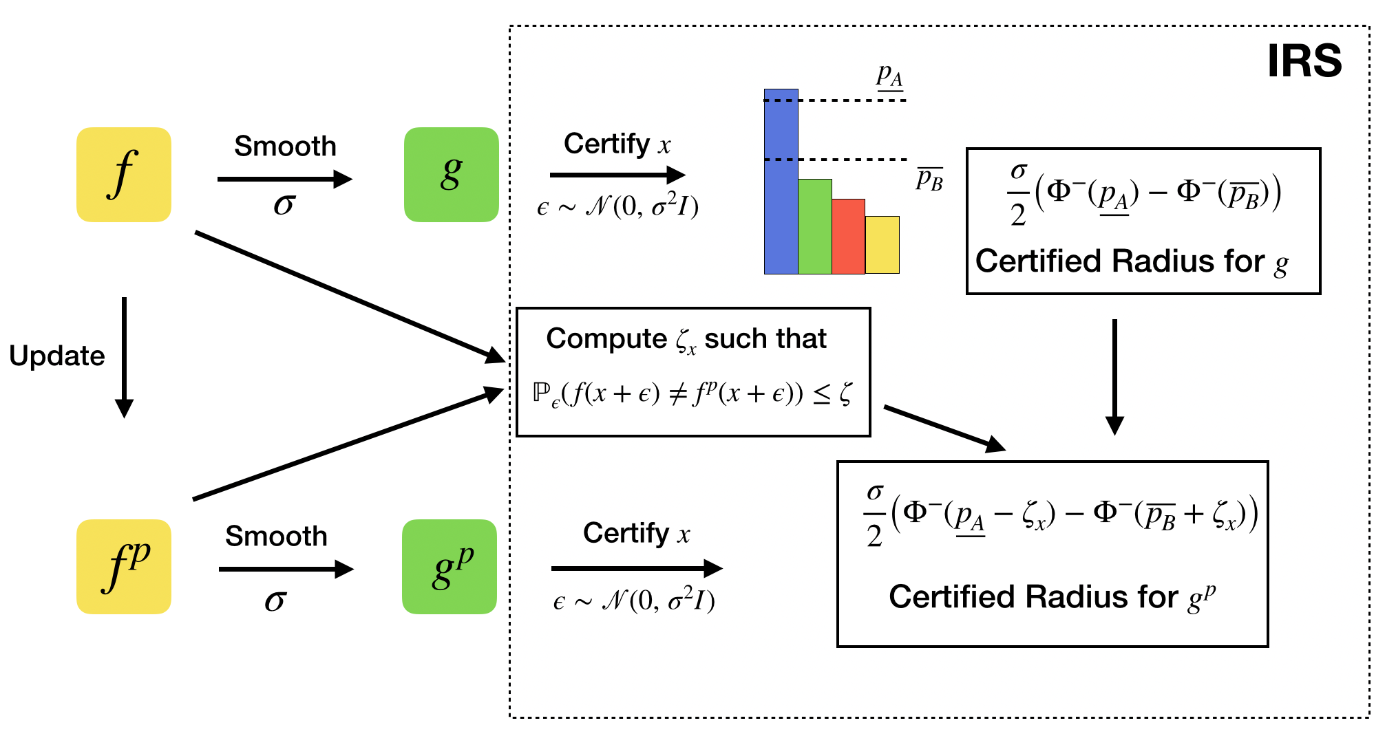
Figure 1: Workflow of IRS from left to right. IRS takes the original classifier $f$ and input $x$. It is built on top of the standard randomized smoothing (RS) framework. IRS reuses the $\underline{p_{A}}$ and $\overline{p_{B}}$ estimates computed for $f$ on $x$ by RS. IRS estimate $\zeta_{x}$ from $f$ and $f^{p}$. For the smoothed classifier $g^{p}$ obtained from the updated classifier $f^{p}$ it computes the certified radius by combining $\underline{p_{A}}$ and $\overline{p_{B}}$ with $\zeta_{x}$.

Figure 1 illustrates the high-level idea behind the workings of IRS. It takes as input the original classifier $f$, the updated classifier $f^{p}$, and an input $x$. Let $g$ and $g^{p}$ denote the smoothed network obtained from $f$ and $f^{p}$ using RS respectively. IRS reuses the $\underline{p_{A}}$ and $\overline{p_{B}}$ estimates computed for $g$ to compute the certified radius for $g^{p}$.

3.1 Motivation

Insight 1: Similarity in approximate networks We observe that for many practical approximations,

Table 1: Average $\zeta_{x}$ with $n=1000$ samples for various approximations.

	CIFAR10	ImageNet
	ResNet-110	ResNet-50
int8	0.009	0.006
prune10	0.01	0.008

$f$ and $f^{p}$ produce the same result on most inputs. In this experiment, we estimate the disparity between $f$ and $f^{p}$ on Gaussian corruptions of the input $x$. We compute a lower confidence bound $\zeta_{x}$ such that $\mathbb{P}_{\epsilon}(f(x+\epsilon)\neq f^{p}(x+\epsilon))\leq\zeta_{x}$ for $\epsilon\sim\mathcal{N}(0,\sigma^{2}I)$.

Table 1 presents empirical average $\zeta_{x}$ for int8 quantization and pruning $10\%$ lowest magnitude weights for some of the networks in our experiments computed over $500$ inputs. We compute $\zeta_{x}$ value as the binomial confidence upper limit using Clopper and Pearson (1934) method with $n=1000$ samples with $\sigma=1$. The results show that the $\zeta_{x}$ value is quite small in all the cases. We present the setup details and results on more networks and approximations Appendix A.4.

Insight 2: Sample reduction through $\zeta_{x}$ estimation We demonstrate that $\zeta_{x}$ estimation for approximate networks is more efficient than running certification from scratch. Fig. 2 shows that for the fixed target error $\chi$, confidence $(1-\alpha)$ and estimation technique, the number of samples required for estimation peaks, when the actual parameter value is around $0.5$ and is smallest around the boundaries. For example, when $\chi=0.5\%$ and $\alpha=0.01$ estimating the unknown binomial proportion will take $41,500$ samples if the actual parameter value is $0.05$ while achieving the same target error and confidence takes $216,900$ samples ($5.22$x higher) if the actual parameter value is $0.5$. As observed in the previous section, $\zeta_{x}$’s value for many practical approximations is close to 0.

Figure 2: The number of samples for the Clopper-Pearson method to achieve a target error $\chi$ with confidence $(1-\alpha)$.

Leveraging the observation shown in Fig. 2 and given actual value $\zeta_{x}$ is close to 0, estimating $\zeta_{x}$ with existing binomial proportion estimation techniques is efficient and requires a smaller number of samples. But this observation does not apply for estimating $\underline{p_{A}}$ and $\overline{p_{B}}$ of smoothed approximate classifier $g^{p}$ where $p_{A}$ and $p_{B}$ may be far from 0 or 1. We show in Appendix A.2 that this observation is not contingent on a specific estimation method and holds for other popular estimation techniques, e.g., (Wilson, 1927), (Agresti and Coull, 1998).

Insight 3: Computing the approximate network’s certified radius using $\zeta_{x}$ For certification of the approximate network $g^{p}$, our main insight is that estimating $\zeta_{x}$ and using that value to compute the certified radius is more efficient than computing RS certified radius from scratch. The next theorem shows how to use estimated value of $\zeta_{x}$ to certify $g^{p}$ (the proof is in Appendix A.1):

[] If a classifier $f^{p}$ is such that for all $x\in\mathbb{R}^{m},\mathbb{P}_{\epsilon}(f(x+\epsilon)\neq f^{p}(x+\epsilon))\leq\zeta_{x}$, and classifier $f$ satisfies $\mathbb{P}_{\epsilon}(f(x+\epsilon)=c_{A})\geq\underline{p_{A}}\geq\overline{p_{B}}\geq\max_{c\neq c_{A}}\mathbb{P}_{\epsilon}(f(x+\epsilon)=c)$ and $\underline{p_{A}}-\zeta_{x}\geq\overline{p_{B}}+\zeta_{x}$ then $g^{p}$ satisfies $g^{p}(x+\delta)=c_{A}$ for all $\delta$ satisying $\|\delta\|_{2}\leq\frac{\sigma}{2}(\Phi^{-1}(\underline{p_{A}}-\zeta_{x})-\Phi^{-1}(\overline{p_{B}}+\zeta_{x}))$

3.2 IRS Certification Algorithm

Algorithm 2 IRS algorithm: Certification with cache

Inputs: $f^{p}$: DNN obtained from approximating $f$, $\sigma$: standard deviation, $x$: input to the DNN, $n_{p}$: number of Gaussian samples used for certification, $\mathcal{C}_{f}$: stores the information to be reused from certification of $f$, $\alpha$ and $\alpha_{\zeta}$: confidence parameters, $\gamma$: threshold hyperparameter to switch between estimation methods

1:function CertifyIRS($f^{p},\sigma,x,n_{p},\mathcal{C}_{f},\alpha,\alpha_{\zeta},\gamma$)

2:  $\hat{c}_{A}\leftarrow\text{top index in }\mathcal{C}_{f}[x]$

3:  $\underline{p_{A}}\leftarrow\text{lower confidence of $f$ from }\mathcal{C}_{f}[x]$

4:  if $\underline{p_{A}}<\gamma$ then

5:    $\zeta_{x}\leftarrow\text{EstimateZeta}(f^{p},\sigma,x,n_{p},\mathcal{C}_{f},\alpha_{\zeta})$

6:    if $\underline{p_{A}}-\zeta_{x}>\frac{1}{2}$ then

7:      return prediction $\hat{c}_{A}$ and radius $\sigma\Phi^{-1}(\underline{p_{A}}-\zeta_{x})$     

8:  else

9:    $counts\leftarrow\text{SampleUnderNoise}(f^{p},x,n_{p},\sigma)$

10:    $p^{\prime}_{A}\leftarrow\text{LowerConfidenceBound}(counts[\hat{c}_{A}],n_{p},1-(\alpha+\alpha_{\zeta}))$

11:    if $p^{\prime}_{A}>\frac{1}{2}$ then

12:      return prediction $\hat{c}_{A}$ and radius $\sigma\Phi^{-1}(p^{\prime}_{A})$       

13:  return ABSTAIN

The Algorithm 2 presents the pseudocode for the IRS algorithm, which extends RS certification from Algorithm 1. The algorithm takes the modified classifier $f^{p}$ and certifies the robustness of $g^{p}$ around $x$. The input $n_{p}$ denotes the number of Gaussian corruptions used by the algorithm.

The IRS algorithm utilizes a cache $\mathcal{C}_{f}$, which stores information obtained from the RS execution of the original classifier $f$ for each input $x$. The cached information is crucial for the operation of IRS. $\mathcal{C}_{f}$ stores the top predicted class index $\hat{c}_{A}$ and its lower confidence bound $\underline{p_{A}}$ for $f$ on input $x$.

The standard RS algorithm takes a conservative value of $\overline{p_{B}}$ by letting $\overline{p_{B}}=1-\underline{p_{A}}$. This works reasonably well in practice and simplifies the computation of certified radius $\frac{\sigma}{2}(\Phi^{-1}(\underline{p_{A}})-\Phi^{-1}(\overline{p_{B}}))$ to $\sigma\Phi^{-1}(\underline{p_{A}})$. We make a similar choice in IRS, which simplifies the certified radius calculation from $\frac{\sigma}{2}(\Phi^{-1}(\underline{p_{A}}-\zeta_{x})-\Phi^{-1}(\overline{p_{B}}+\zeta_{x}))$ of Theorem 2 to $\sigma\Phi^{-1}(\underline{p_{A}}-\zeta_{x})$ as we state in the next theorem (the proof is in Appendix A.1):

[] If $\underline{p_{A}}-\zeta_{x}\geq\frac{1}{2},$ then $\sigma\Phi^{-1}(\underline{p_{A}}-\zeta_{x})\leq\frac{\sigma}{2}(\Phi^{-1}(\underline{p_{A}}-\zeta_{x})-\Phi^{-1}(\overline{p_{B}}+\zeta_{x}))$

As per our insight 2 (Section 3.1), binomial confidence interval estimation requires fewer samples for binomial with actual probability close to $0$ or $1$. IRS can take advtange of this when $\underline{p_{A}}$ is not close to $1$. However, when $\underline{p_{A}}$ is close to $1$ then there is no benefit of using $\zeta_{x}$-based certified radius for $g^{p}$. Therefore, the algorithm uses a threshold hyperparameter $\gamma$ close to $1$ that is used to switch between certified radius from Theorem 2 and standard RS from Theorem 2.

If the $\underline{p_{A}}$ is less than the threshold $\gamma$, then an estimate of $\zeta_{x}$ for approximate classifier $f^{p}$ and the original classifier $f$ is computed using the EstimateZeta function. We disucss EstimateZeta procedure in the next section. If the $\underline{p_{A}}-\zeta_{x}$ is greater than $\frac{1}{2}$, then the top predicted class in the cache is returned as the prediction with the radius $\sigma\Phi^{-1}(\underline{p_{A}}-\zeta_{x})$ as computed in Theorem 3.2.

In case, if $\underline{p_{A}}$ is greater than the threshold $\gamma$, similar to standard RS, the IRS algorithm draws $n^{p}$ samples of $f^{p}(x+\epsilon)$ by running $n^{p}$ noise-corrupted copies of $x$ through the classifier $f^{p}$. The function $\text{SampleUnderNoise}(f^{p},x,n_{p},\sigma)$ in the pseudocode draws $n_{p}$ samples of noise, $\epsilon_{1}\dots\epsilon_{n_{p}}\sim\mathcal{N}(0,\sigma^{2}I)$, runs each $x+\epsilon_{i}$ through the classifier $f^{p}$, and returns a vector of class counts. Again, if the lower confidence bound is greater than $\frac{1}{2}$, the top predicted class is returned as the prediction with a radius based on the lower confidence bound $\underline{p_{A}}$.

If the function does certify the input in both of the above cases, it returns ABSTAIN.

The hyperparameters $\alpha$ and $\alpha_{\zeta}$ denote confidence of IRS results. The IRS algorithm results are correct with confidence at least $1-(\alpha+\alpha_{\zeta})$. For the case $\underline{p_{A}}\geq\gamma$, this holds since we follow the same steps as standard RS. The function $\text{LowerConfidenceBound}(counts[\hat{c}_{A}],n_{p},1-(\alpha+\alpha_{\zeta}))$ in the pseudocode returns a one-sided $1-(\alpha+\alpha_{\zeta})$ lower confidence interval for the Binomial parameter $p$ given a sample $counts[\hat{c}_{A}]\sim Binomial(n_{p},p)$. We next state the theorem that shows the confidence of IRS results in the other case when $\underline{p_{A}}<\gamma$ (the proof is in Appendix A.1):

[] If $\mathbb{P}_{\epsilon}(f(x+\epsilon)=f^{p}(x+\epsilon))>1-\zeta_{x}$ with confidence at least $1-\alpha_{\zeta}$. If classifier $f$ satisfies $\mathbb{P}_{\epsilon}(f(x+\epsilon)=c_{A})\geq\underline{p_{A}}$ with confidence at least $1-\alpha$. Then for classifier $f^{p}$, $\mathbb{P}_{\epsilon}(f^{p}(x+\epsilon)=c_{A})\geq\underline{p_{A}}-\zeta_{x}$ with confidence at least $1-(\alpha+\alpha_{\zeta})$

3.3 Estimating the Upper Confidence Bound $\zeta_{x}$

In this section, we present our method for estimating $\zeta_{x}$ such that $\mathbb{P}_{\epsilon}(f(x+\epsilon)\neq f^{p}(x+\epsilon))\leq\zeta_{x}$ with high confidence (Algorithm 3). We use the Clopper-Pearson Clopper and Pearson (1934) method to estimate the upper confidence bound $\zeta_{x}$.

Algorithm 3 Estimate $\zeta_{x}$

Inputs: $f^{p}$: DNN obtained from approximating $f$, $\sigma$: standard deviation, $x$: input to the DNN, $n_{p}$: number of Gaussian samples used for estimating $\zeta_{x}$, $\mathcal{C}_{f}$: stores the information to be reused from certification of $f$, $\alpha_{\zeta}$: confidence parameter
Output: Estimated value of $\zeta_{x}$

1:function EstimateZeta($f^{p},\sigma,x,n_{p},\mathcal{C}_{f},\alpha_{\zeta}$)

2:  $n_{\Delta}\leftarrow 0$

3:  $\textit{seeds}\leftarrow$ seeds for original samples from $\mathcal{C}_{f}[x]$

4:  $\textit{predictions}\leftarrow f$’s predictions on samples from $\mathcal{C}_{f}[x]$

5:  for i $\in\{1,\dots n_{p}\}$ do

6:    $\epsilon\sim\mathcal{N}(0,\sigma^{2}I)$ using $\textit{seeds}[i]$

7:    $c_{f}\leftarrow\textit{predictions}[i]$

8:    $c_{f^{p}}\leftarrow f^{p}(x+\epsilon)$

9:    $n_{\Delta}\leftarrow n_{\Delta}+I(c_{f}\neq c_{f^{p}})$   

10:  return UpperConfidenceBound($n_{\Delta}$, $n_{p}$, $1-\alpha_{\zeta}$)

We store the seeds used for randomly generating Gaussian samples while certifying the function $f$ in the cache, and we reuse these seeds to generate the same Gaussian samples. $\textit{seeds}[i]$ stores the seed used for generating $i$-th sample in the RS execution of $f$, and $\textit{predictions}[i]$ stores the prediction of $f$ on the corrsponding $x+\epsilon$. We evaluate $f^{p}$ on each corruption $\epsilon$ generated from seeds and match them to predictions by $f$. $c_{f}$ and $c_{f^{p}}$ represent the top class prediction by $f$ and $f^{p}$ respectively. $n_{\Delta}$ is the count of the number of corruptions $\epsilon$ such that $f$ and $f^{p}$ do not match on $x+\epsilon$.

The function UpperConfidenceBound($n_{\Delta}$, $n_{p}$, $1-\alpha_{\zeta}$) in the pseudocode returns a one-sided $1-\alpha_{\zeta}$ upper confidence interval for the Binomial parameter $p$ given a sample $n_{\Delta}\sim Binomial(n_{p},p)$. Storing the seeds used for generating noisy samples in the cache results in negligible memory overhead. Theorem 3.2 does not make any assumptions about the independence of the estimation of $\underline{p_{A}}$ and $\zeta_{x}$, thus we can reuse the same Gaussian samples for both estimations.

4 Experimental Methodology

Networks and Datasets. We evaluate IRS on CIFAR-10 (Krizhevsky et al., ) and ImageNet (Deng et al., 2009). On each dataset, we use several classifiers, each with a different $\sigma$’s. For an experiment that adds Gaussian corruptions with $\sigma$ to the input, we use the network that is trained with Gaussian augmentation with variance $\sigma^{2}$. On CIFAR-10 we use the base classifier a 20-layer and 110-layer residual network. On ImageNet our base classifier is a ResNet-50.

Network Approximations. We evaluate IRS on multiple approximations. We consider float16 (fp16), bfloat16 (bf16), and int8 quantizations (Section 5.1). We show the effectiveness of IRS on pruning approximation in Section 5.2. For int8 quantization, we use dynamic per-channel quantization mode. from (Paszke et al., 2019) library. For float16 and bfloat16 quantization, we change the data type of the DNN weights from float32 to the respective types. For the pruning experiment, we perform the lowest weight magnitude (LWM) pruning. The top-1 accuracy of the networks used in the evaluation and the approximate networks is discussed in Appendix A.3.

Experimental Setup. We ran experiments on a 48-core Intel Xeon Silver 4214R CPU with 4 NVidia A100 GPUs. IRS is implemented in Python and uses PyTorch (Paszke et al., 2019) library.

Hyperparameters. We use confidence parameters $\alpha=0.001$ for the original certification, and $\alpha_{\zeta}=0.001$ for the estimation of $\zeta_{x}$. To establish a fair comparison, we set the baseline confidence with $\alpha_{b}=\alpha+\alpha_{\zeta}=0.002$. This choice ensures that both the baseline and IRS, provide certified radii with equal confidence. We use grid search to choose an effective value for $\gamma$. A detailed description of our hyperparameter search and its results are described in Section 5.3.

Average Certified Radius. We compute the certified radius $r$ when the certification algorithm did not abstain and returned the correct class with radius $r$, for both IRS (Algorithm 2) and the baseline (Algorithm 1). In other cases, we say that the certified radius $r=0$. We compute the average certified radius (ACR) by taking the mean of certified radii computed for inputs in the test set. Higher ACR indicates stronger robustness certification guarantees.

5 Experimental Results

We now present our main evaluation results. In all of our experiments, we follow a specific procedure:

1. We certify the original smoothed classifier $g$ using standard RS with a sample size of $n$.

2. We approximate the base classifier $f$ with $f^{p}$.

3. Using the IRS, we certify smoothed classifier $g^{p}$ by employing Algorithm 2 and utilizing the cached information $\mathcal{C}_{f}$ obtained from the certification of $g$.

We compare IRS to the baseline approach, which uses standard non-incremental RS (Algorithm 1), to certify $g^{p}$. Our results compare the ACR and the average certification time between IRS and the baseline for various values of $n_{p}$.

5.1 IRS speedups on quantization

We compare the ACR of the baseline and IRS for different DNN quantizations. We use $n=10^{4}$ for samples for certification of $g$. For certifying $g^{p}$, we consider $n^{p}$ values from $\{1\%,\dots 10\%\}$ of $n$. For CIFAR10, we consider $\sigma\in\{0.25,0.5,1.0$}, similar to previous work Cohen et al. (2019). For ImageNet, we consider $\sigma\in\{0.5,1.0,2.0\}$. We perform experiments on $500$ images and compute the average certification time.

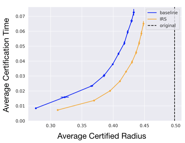
(a) ResNet-20, CIFAR10, $\sigma=0.5$

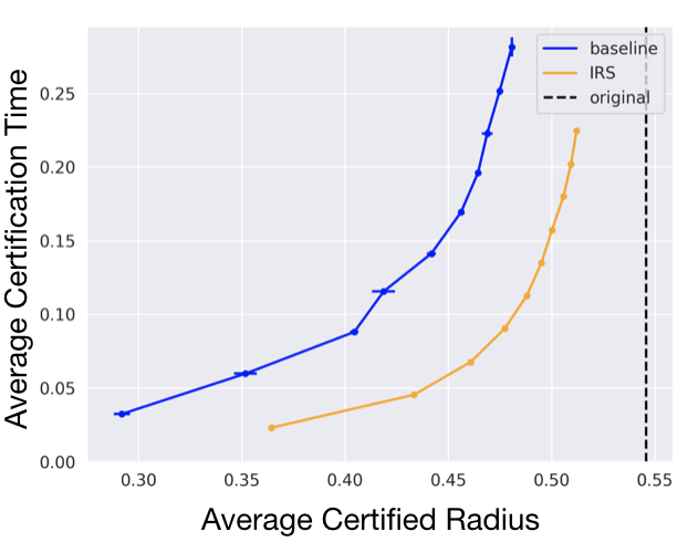
(b) ResNet-110, CIFAR10, $\sigma=1.0$

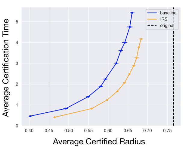
(c) ResNet-50, ImageNet, $\sigma=2.0$

Figure 3: Average certified radius (ACR) vs average certification time for the network with int8 quantization. x-axis and y-axis error bars are based on standard deviation.

Figure 3 presents the comparison between IRS and RS. The x-axis displays the ACR and the y-axis displays the average certification time. The plot consists of 10 markers each for the IRS and the baseline representing a specific value of $n_{p}$. Expectedly, the higher the value of $n_{p}$, the higher the average time and ACR. The marker coordinate denotes the ACR and the average time for an experiment. In all the cases, IRS consistently takes less certification time to obtain the same ACR.

Figure 3(a), for ResNet-20 on CIFAR10, shows that IRS gives 1.66x to 1.87x speedup for a given ACR. Figure 3(b), for ResNet-110 on CIFAR10, shows that IRS gives 2.44x to 2.86x speedup. Moreover, we see that IRS achieves an ACR of more than 0.5 in 0.15s on average, whereas the baseline does not reach above 0.5 ACR for any of the $n_{p}$ values in our experiments.

Figure 3(c), for ResNet-50 on ImageNet, shows that IRS gives 1.6x to 2.05x speedup for a given ACR. For most inputs, we observe that IRS certifies a higher radius than the baseline. For CIFAR10 with ResNet-110 with $\sigma=1$, for 41% of the inputs IRS certifies a larger radius, for 52% of inputs it certifies an equal radius, and for only 6% inputs it certifies a smaller radius than the baseline.

Table 2: Average IRS speedup for combinations of quantizations and $\sigma$’s.

Dataset	Architecture	$\sigma$	Quantization
			fp16	bf16	int8
		0.25	1.37x	1.29x	1.3x
CIFAR10	ResNet-20	0.5	1.79x	1.7x	1.77x
		1.0	2.85x	2.41x	2.65x
		0.25	1.42x	1.35x	1.29x
CIFAR10	ResNet-110	0.5	1.97x	1.74x	1.77x
		1.0	3.02x	2.6x	2.6x
		0.5	1.2x	1.14x	1.19x
ImageNet	ResNet-50	1.0	1.43x	1.31x	1.43x
		2.0	2.04x	1.69x	1.80x

To quantify the speedup achieved by IRS over the baseline, we employ an approximate area under the curve (AOC) analysis. Specifically, we plot the average certification time against the ACR. In most cases, IRS certifies a larger ACR compared to the baseline, resulting in regions on the x-axis where IRS exists but the baseline does not. To ensure a conservative estimation, we calculate the speedup only within the range where both IRS and the baseline exist. We determine the speedup by computing the ratio of the AOC for IRS to the AOC for the baseline within this common range. Table 2 summarizes the average speedups. Plots for other experiments with all combinations of networks, $\sigma$, and quantizations are in Appendix A.7.

Effect of standard deviation $\sigma$ on IRS speedup. We observe that IRS gets a larger speedup for smoothing with larger $\sigma$. Figure 4, presents the $\underline{p_{A}}$ distribution between $0.5$ to $1$, for ResNet-110 on CIFAR-10. The x-axis represents the range of $\underline{p_{A}}$ values and the y-axis represents their respective proportion. The results show that while certifying larger $\sigma$, on average the $\underline{p_{A}}$ values are smaller. As shown in Figure 4(a), for $\sigma=0.25$, less than $35\%$ of $\underline{p_{A}}$ values are smaller than $0.95$. On the other hand, in Figure 4(b), when $\sigma=1.0$, the distribution is less left-skewed as nearly $75\%$ of $\underline{p_{A}}$ values are less than $0.95$. When the $\sigma$ is larger, the values of $\underline{p_{A}}$ tend to be farther away from 1. Therefore, the estimation of $\underline{p_{A}}$ is less precise in such cases, as observed in insight 2. As a result, non-incremental RS performs poorly compared to IRS in these situations, leading to a greater speedup with IRS.

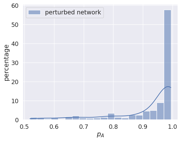
(a) ResNet-110 on CIFAR-10 ($\sigma=0.25$)

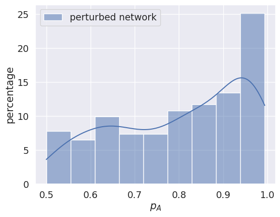
(b) ResNet-110 on CIFAR-10 ($\sigma=1.0$)

Figure 4: Distribution of $\underline{p_{A}}$ values greater than 0.5 with different $\sigma$ for ResNet-110 on CIFAR-10.

5.2 IRS speedups on Pruned Models

In this experiment, we show IRS’s ability to certify pruned networks. We employ $l_{1}$ unstructured pruning, which prunes the fraction of the lowest $l_{1}$ magnitude weights from the network. Table 4 presents the average IRS speedup for networks obtained by pruning $5\%,10\%$ and $20\%$ weights. The speedups range from 0.99x to 2.7x. As the network is pruned more aggressively, it is expected that the speedup achieved by IRS will be lower. This is due to higher values of $\zeta_{x}$ associated with aggressive pruning. In Appendix A.4, we provide average $\zeta_{x}$ values for all approximations. In comparison to pruning, quantization typically yields smaller $\zeta_{x}$ values, making IRS more effective for quantization.

Table 3: Average IRS speedup for combinations of pruning ratio and $\sigma$’s.

Dataset	Architecture	$\sigma$	Prune
			5%	10%	20%
		0.25	1.3x	1.25x	0.99x
CIFAR10	ResNet-20	0.5	1.63x	1.39x	1.13x
		1.0	2.5x	2.09x	1.39x
		0.25	1.35x	1.24x	1.04x
CIFAR10	ResNet-110	0.5	1.83x	1.6x	1.23x
		1.0	2.7x	2.25x	1.63x
		0.5	1.19x	1.04x	0.87x
ImageNet	ResNet-50	1.0	1.36x	1.15x	0.87x
		2.0	1.87x	1.54x	1.01x

Table 4: Average IRS speedup for combinations of $n$, $\sigma$’s, and quantizations for ResNet-20 on CIFAR10.

$n$	$\sigma$	Quantization
		fp16	bf16	int8
	0.25	1.37x	1.29x	1.3x
$10^{4}$	0.5	1.79x	1.7x	1.77x
	1.0	2.85x	2.41x	2.65x
	0.25	1.22x	1.11x	1.27x
$10^{5}$	0.5	1.73x	1.4x	1.86x
	1.0	3.88x	2.40x	4.31x
	0.25	1.12x	0.93x	1.15x
$10^{6}$	0.5	1.97x	1.04x	2.25x
	1.0	4.58x	1.25x	5.85x

5.3 Ablation Studies

Sensitivity to changing $n$. In Section 5, to save time due to a large number of approximations and networks tested, we used $n=10^{4}$ samples for the certification of $g$. Here, we present the effect of certifying with a larger $n$ by comparing the ACR vs average certification time on the IRS and baseline approaches for a ResNet-20 base classifier on CIFAR10. On average, for larger $n$, we demonstrate greater speedup for larger $\sigma$. For instance, for int8 quantization with $\sigma=1.0$, the speedup for certifying with $n=10^{6}$ samples was $5.85$x as compared to certification with $n=10^{4}$ which yielded at $2.65$x speedup. However, for smaller $\sigma$, certification with a larger n results in less speedup. For $\sigma=0.25$, we observe speedups ranging from $1.29$x to $1.37$x for $n=10^{4}$ whereas from $0.93$x to $1.15$x for $n=10^{6}$.

Table 5: ACR for each $\gamma$.

$\gamma$	CIFAR10	CIFAR10	ImageNet
	ResNet-20	ResNet-110	ResNet-50
0.9	0.438	0.436	0.458
0.95	0.442	0.439	0.464
0.975	0.445	0.441	0.465
0.99	0.446	0.443	0.466
0.995	0.445	0.442	0.467
0.999	0.444	0.442	0.464

Sensitivity to threshold $\gamma$. For each network architecture, we chose the hyperparameter $\gamma$ by running IRS to certify a small subset of the validation set images for certifying the int8 quantized network. We use the same $\gamma$ for each network irrespective of the approximation and $\sigma$. We use the grid search to choose the best value of gamma from the set $\{0.9,0.95,0.975,0.99,0.999\}$. Table 5 presents the ACR obtained for each $\gamma$. For CIFAR10 networks we chose $\gamma$ as $0.99$ and for the ImageNet networks, we chose $0.995$ since they result in the highest ACR.

6 Related Work

Incremental Program Verification. The scalability of traditional program verification has been significantly improved by incremental verification, which has been applied on an industrial scale (Johnson et al., 2013; Lakhnech et al., 2001; O’Hearn, 2018; Stein et al., 2021). Incremental program analysis tasks achieve faster analysis of individual commits by reusing partial results (Yang et al., 2009), constraints (Visser et al., 2012), and precision information (Beyer et al., 2013) from previous runs.

Incremental DNN Certification. Several methods have been introduced in recent years to certify the properties of DNNs deterministically (Tjeng et al., 2017; Bunel et al., 2020; Katz et al., 2017; Wang et al., 2021b; Laurel et al., 2022) and probabilisticly (Cohen et al., 2019). More recently, researchers used incremental certification to improve the scalability of DNN certification (Fischer et al., 2022b; Ugare et al., 2022; Wei and Liu, 2021; Ugare et al., 2023) – these works apply complete and incomplete deterministic certification using formal logic cannot scale to e.g., ImageNet. In contrast, we propose incremental probabilistic certification with Randomized Smoothing, which enables much greater scalability.

Randomized Smoothing. Cohen et al. (2019) introduced the addition of Gaussian noise to achieve $l_{2}$-robustness results. Several extensions to this technique utilize different types of noise distributions and radius calculations to determine certificates for general $l_{p}$-balls. Yang et al. (2020) and Zhang et al. (2020) derived recipes for determining certificates for $p=1,2$, and $\infty$. Lee et al. (2019), Wang et al. (2021a), and Schuchardt et al. (2021) presented extensions to discrete perturbations such as $l_{0}$-perturbations, while Bojchevski et al. (2023), Gao et al. (2020), Levine and Feizi (2020), and Liu et al. (2021) explored extensions to graphs, patches, and point cloud manipulations. Dvijotham et al. (2020) presented theoretical derivations for the application of both continuous and discrete smoothing measures, while Mohapatra et al. (2020) improved certificates by using gradient information. Horváth et al. (2022) used ensembles to improve the certificate.

Beyond norm-balls certificates, Fischer et al. (2020) and Li et al. (2021) presented how geometric operations such as rotation or translation can be certified via Randomized Smoothing. yeh Chiang et al. (2022) and Fischer et al. (2022a) demonstrated how the certificates can be extended from the setting of classification to regression (and object detection) and segmentation, respectively. For classification, Jia et al. (2020) extended certificates from just the top-1 class to the top-k classes, while Kumar et al. (2020) certified the confidence of the classifier, not just the top-class prediction. Rosenfeld et al. (2020) used Randomized Smoothing to defend against data poisoning attacks. These RS extensions (using different noise distributions, perturbations, and geometric operations) are orthogonal to the standard RS approach from Cohen et al. (2019). While these extensions have been shown to improve the overall bredth of RS, IRS is complementary to these extensions. We believe that IRS has the potential to accelerate the incremental certification process in settings where these extensions are employed, but leave investigating these extensions for future work.

7 Limitations

We showed that IRS is effective at certifying smoothed version of approximated DNN. However, there are certain limitations to the effectiveness of IRS.

As the level of approximation increases, the ability of IRS to provide efficient recertification decreases. As observed in Section 5.1 and Section 5.2, IRS is more effective on quantization compared to pruning since it results in smaller $\zeta_{x}$ values. We apply IRS on the common pruning and quantization approximations. However, we do not theoretically characterize the set of all approximations where IRS is applicable. We leave it to future work.

The smoothing parameter $\sigma$ used in IRS affects its efficiency, with larger values of $\sigma$ generally leading to better results. As a consequence, we observed a smaller speedup when using a smaller value of $\sigma$ (e.g., 0.25 on CIFAR10) compared to a larger value (e.g., 1 on CIFAR10). The value of $\sigma$ offers a trade-off between robustness and accuracy. By choosing a larger $\sigma$, one can improve robustness but it may lead to a loss of accuracy in the model.

IRS targets fast certification while maintaining a sufficiently large radius. Therefore, we considered $n_{p}$ in the range $\{1\%\dots 10\%\}$ of $n$ for our evaluation. However, IRS certified radius can be smaller than the non-incremental RS, provided the user has a larger sample budget. In our experiment in Appendix A.5 we test IRS on larger $n_{p}$ and observe that IRS is better than baseline for $n_{p}$ less than $70\%$ of $n$. This is particularly advantageous when computational resources are limited, allowing for more efficient certification.

Limitations of RS, such as (1) the statistical nature of the method, introduces the possibility that the certification may not always hold. (2) the limitations of training for RS (3) impact on class-wise accuracy Mohapatra et al. (2021), are applicable to IRS as well.

8 Conclusion

We propose IRS, the first incremental approach for probabilistic DNN certification. IRS leverages the certification guarantees obtained from the original smoothed model to certify a smoothed approximated model with very few samples. Reusing the computation of original guarantees significantly reduces the computational cost of certification while maintaining strong robustness guarantees. IRS speeds up certification up to 3x over the standard non-incremental RS baseline on state-of-the-art classification models. We believe that our approach will pave the way for more efficient and effective certification of DNNs in real-world applications.

Appendix A Appendix

A.1 Theorems

See 2

Proof.

If $f(x+\epsilon)=c_{A}$ and $f^{p}(x+\epsilon)=f(x+\epsilon)$ then $f^{p}(x+\epsilon)=c_{A}$.
Thus, if $f^{p}(x+\epsilon)\neq c_{A}$ then $f(x+\epsilon)\neq c_{A}$ or $f^{p}(x+\epsilon)\neq f(x+\epsilon)$.
Using union bound,

$$\mathbb{P}_{\epsilon}(f^{p}(x+\epsilon)\neq c_{A})\leq\mathbb{P}_{\epsilon}(f(x+\epsilon)\neq c_{A})+\mathbb{P}_{\epsilon}(f(x+\epsilon)\neq f^{p}(x+\epsilon))$$

$$(1-\mathbb{P}_{\epsilon}(f^{p}(x+\epsilon)=c_{A}))\leq(1-\mathbb{P}_{\epsilon}(f(x+\epsilon)=c_{A}))+\mathbb{P}_{\epsilon}(f(x+\epsilon)\neq f^{p}(x+\epsilon))$$

$$\mathbb{P}_{\epsilon}(f(x+\epsilon)=c_{A})\leq\mathbb{P}_{\epsilon}(f^{p}(x+\epsilon)=c_{A})+\mathbb{P}_{\epsilon}(f(x+\epsilon)\neq f^{p}(x+\epsilon))$$

$$\underline{p_{A}}-\zeta_{x}\leq\mathbb{P}_{\epsilon}(f^{p}(x+\epsilon)=c_{A})$$

Similarly, if $f(x+\epsilon)\neq c$ then $f^{p}(x+\epsilon)\neq c$ or $f^{p}(x+\epsilon)\neq f(x+\epsilon)$.
Hence, using union bound,

$$\mathbb{P}_{\epsilon}(f(x+\epsilon)\neq c)\leq\mathbb{P}_{\epsilon}(f^{p}(x+\epsilon)\neq c)+\mathbb{P}_{\epsilon}(f(x+\epsilon)\neq f^{p}(x+\epsilon))$$

$$(1-\mathbb{P}_{\epsilon}(f(x+\epsilon)=c))\leq(1-\mathbb{P}_{\epsilon}(f^{p}(x+\epsilon)=c))+\mathbb{P}_{\epsilon}(f(x+\epsilon)\neq f^{p}(x+\epsilon))$$

$$\mathbb{P}_{\epsilon}(f^{p}(x+\epsilon)=c)\leq\mathbb{P}_{\epsilon}(f(x+\epsilon)=c)+\mathbb{P}_{\epsilon}(f(x+\epsilon)\neq f^{p}(x+\epsilon))$$

$$\max_{c\neq c_{A}}\mathbb{P}_{\epsilon}(f^{p}(x+\epsilon)=c)\leq\max_{c\neq c_{A}}\mathbb{P}_{\epsilon}(f(x+\epsilon)=c)+\zeta_{x}$$

$$\max_{c\neq c_{A}}\mathbb{P}_{\epsilon}(f^{p}(x+\epsilon)=c)\leq\overline{p_{B}}+\zeta_{x}$$

Hence, using Theorem 2, $g^{p}$ satisfies $g^{p}(x+\delta)=c_{A}$ for all $\delta$ satisying $\|\delta\|_{2}\leq\frac{\sigma}{2}(\Phi^{-1}(\underline{p_{A}}-\zeta_{x})-\Phi^{-1}(\overline{p_{B}}+\zeta_{x}))$

∎

See 3.2

Proof.

Since $\underline{p_{A}}-\zeta_{x}\geq\frac{1}{2}$, $0\leq\underline{p_{A}}\leq 1$ and $\zeta_{x}\geq 0$, we get $0\leq\underline{p_{A}}-\zeta_{x}\leq 1$

And since $1-\underline{p_{A}}\geq\overline{p_{B}}$, we get $\overline{p_{B}}+\zeta_{x}\leq\frac{1}{2}$, and thus, $0\leq\overline{p_{B}}+\zeta_{x}\leq 1$

Since $\Phi^{-1}(1-t)=-\Phi^{-1}(t)$

$$\Phi^{-1}(\overline{p_{B}}+\zeta_{x})=-\Phi^{-1}(1-(\overline{p_{B}}+\zeta_{x}))$$

$$=-\Phi^{-1}((1-\overline{p_{B}})-\zeta_{x})$$

Since $1-\underline{p_{A}}\geq\overline{p_{B}}$

$$\leq-\Phi^{-1}(\underline{p_{A}}-\zeta_{x})$$

Hence,

$$\Phi^{-1}(\underline{p_{A}}-\zeta_{x})\leq-\Phi^{-1}(\overline{p_{B}}+\zeta_{x})$$

$$\frac{\sigma}{2}\Phi^{-1}(\underline{p_{A}}-\zeta_{x})\leq-\frac{\sigma}{2}\Phi^{-1}(\overline{p_{B}}+\zeta_{x})$$

Adding $\frac{\sigma}{2}\Phi^{-1}(\underline{p_{A}}-\zeta_{x})$ on both sides,

$$\sigma\Phi^{-1}(\underline{p_{A}}-\zeta_{x})\leq\frac{\sigma}{2}(\Phi^{-1}(\underline{p_{A}}-\zeta_{x})-\Phi^{-1}(\overline{p_{B}}+\zeta_{x}))$$

∎

See 3.2

Proof.

Suppose $f$ and $f^{p}$ are classifiers such that for all $x\in\mathbb{R}^{m},\mathbb{P}_{\epsilon}(f(x+\epsilon)=c_{A})\geq\underline{p_{A}}$ and $\mathbb{P}_{\epsilon}(f(x+\epsilon)=f^{p}(x+\epsilon))>1-\zeta_{x}$.
Let $E_{1}$ denote the event that $\mathbb{P}_{\epsilon}(f(x+\epsilon)=c_{A})\geq\underline{p_{A}}$.
Let $E_{2}$ denote the event that $\mathbb{P}_{\epsilon}(f(x+\epsilon)=f^{p}(x+\epsilon))>1-\zeta_{x}$.
By Theorem 2,

$$\mathbb{P}_{\epsilon}(f(x+\epsilon)=c_{A})\leq\mathbb{P}_{\epsilon}(f^{p}(x+\epsilon)=c_{A})+\mathbb{P}_{\epsilon}(f(x+\epsilon)\neq f^{p}(x+\epsilon))$$

$$\underline{p_{A}}-\zeta_{x}\leq\mathbb{P}_{\epsilon}(f^{p}(x+\epsilon)=c_{A})$$

Let $E_{3}$ denote the event that $\underline{p_{A}}-\zeta_{x}\leq\mathbb{P}_{\epsilon}(f^{p}(x+\epsilon)=c_{A})$
Since, $E_{1}$ and $E_{2}$ imply $E_{3}$ i.e. $E_{1}\cap E_{2}\subseteq E_{3}$,

$$\mathbb{P}(E_{3})\geq\mathbb{P}(E_{1}\cap E_{2})$$

By the additive rule of probability,

$$\mathbb{P}(E_{1}\cap E_{2})=\mathbb{P}(E_{1})+\mathbb{P}(E_{2})-\mathbb{P}(E_{1}\cup E_{2})$$

$$\mathbb{P}(E_{3})\geq(1-\alpha)+(1-\alpha_{\zeta})-1$$

$$\mathbb{P}(E_{3})\geq 1-(\alpha+\alpha_{\zeta})$$

Hence, for classifier $f^{p}$, $\mathbb{P}_{\epsilon}(f^{p}(x+\epsilon)=c_{A})\geq\underline{p_{A}}-\zeta_{x}$ has confidence at least $1-(\alpha+\alpha_{\zeta})$ ∎

A.2 Observation for Binomial Confidence Interval Methods

In this section, we show the plots for the number of samples required to estimate an unknown binomial proportion parameter through two popular estimation techniques - the Wilson  [Wilson, 1927] and Agresti-Coull method  [Agresti and Coull, 1998]. For this experiment, we use three different values of the target error $\chi$ = 0.5 %, 0.75 %, and 1.0 % and a fixed confidence value $(1-\alpha)=0.99$ for both estimation methods. As shown in Fig 5, for a fixed target error $\chi$, confidence $(1-\alpha)$, and estimation technique, the number of samples required for estimation peaks, when the actual parameter value is around $0.5$ and is the smallest around the boundaries. This is consistent with the observation described in Section 3.1.

(a) Agresti-Coull method

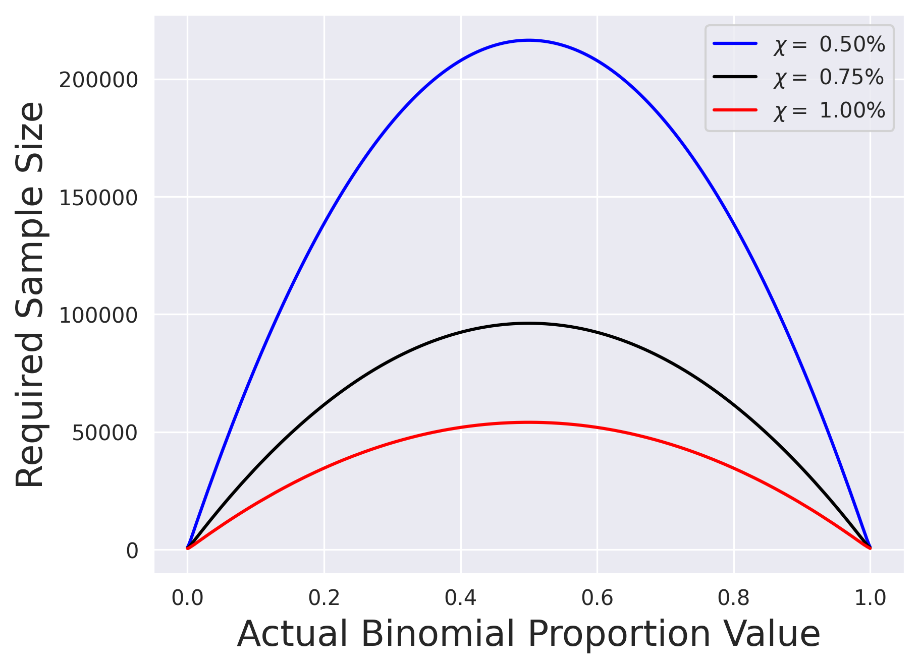
(b) Wilson method

Figure 5: The number of samples for the Agresti-Coull and Wilson method to achieve a target error $\chi$ with confidence $(1-\alpha)$ where $\alpha=0.01$. The plots show that the number of required samples for different methods peaks at 0.5 and decreases towards the boundaries.

A.3 Evaluation Networks

Table 6 and Table 7 respectively present the standard top-1 accuracy of the original and approximated base classifiers and smoothed classifiers respectively.

Table 6: Standard top-1 accuracy for (non-smoothed) networks for combinations of approximations and $\sigma$’s.

Dataset	Architecture	$\sigma$	original	Quantization			Prune
				fp16	bf16	int8	5%	10%	20%
		0.25	67.2	67.2	66.8	67.2	67.4	66.6	66.6
CIFAR10	ResNet-20	0.5	56.8	56.8	57.2	56.8	57	57.4	58
		1.0	47.2	47.2	47.0	47.2	47	46.2	45.2
		0.25	69.0	69.0	69.4	69.0	69.2	68.8	68.2
CIFAR10	ResNet-110	0.5	59.4	59.4	59.4	59.4	59.6	59	58.8
		1.0	47.0	47.0	46.8	46.8	46.8	47.2	47
		0.5	24.2	24.2	24.4	24.2	24.2	24.4	24.2
ImageNet	ResNet-50	1.0	9.6	9.6	9.6	9.6	9.6	9.6	9.6
		2.0	6.4	6.4	6.4	6.4	6.4	6.4	6.4

Table 7: standard top-1 accuracy for smoothed networks for combinations of approximations and $\sigma$’s.

Dataset	Architecture	$\sigma$	original	Quantization			Prune
				fp16	bf16	int8	5%	10%	20%
		0.25	77.2	77	77.2	77.2	77.6	77.2	77.6
CIFAR10	ResNet-20	0.5	67.8	67.4	67.8	67.8	67.8	67.4	67.8
		1.0	55.6	55.6	55.6	55.8	54.8	55.2	55.6
		0.25	76.6	76.4	76.2	76.4	76.2	76.2	76.4
CIFAR10	ResNet-110	0.5	66.2	67	68	66.4	67	66.8	66.6
		1.0	55.6	55.4	56.2	56.2	55	55	54.8
		0.5	63.8	63.4	63.2	63.4	63.6	64	63
ImageNet	ResNet-50	1.0	48.8	48.6	48.8	48.6	48.8	48.6	47.8
		2.0	34.4	34.2	33.8	34.2	34.2	34.4	33.4

A.4 $\zeta_{x}$ evaluation

We compute $\zeta_{x}$ value as the binomial confidence upper limit using Clopper and Pearson [1934] method with $n=1000$ samples. For experiement that adds Gaussian corruptions with $\sigma$ to the input, we use the network that is trained with Gaussian data augmentation with variance $\sigma^{2}$.

Table 8: $\zeta_{x}$ for approximate networks trained on different Gaussian augmentation $\sigma$’s.

Dataset	Architecture	$\sigma$	Quantization			Prune
			fp16	bf16	int8	5%	10%	20%
		0.25	0.01	0.01	0.006	0.01	0.02	0.04
CIFAR10	ResNet-20	0.5	0.006	0.008	0.01	0.01	0.02	0.03
		1.0	0.006	0.007	0.006	0.007	0.02	0.02
		0.25	0.006	0.01	0.006	0.009	0.02	0.04
CIFAR10	ResNet-110	0.5	0.006	0.006	0.006	0.008	0.02	0.03
		1.0	0.006	0.008	0.009	0.007	0.01	0.02
		0.5	$0.006$	0.009	$0.006$	0.01	0.02	0.09
ImageNet	ResNet-50	1.0	$0.007$	0.01	$0.006$	0.01	0.02	0.08
		2.0	$0.006$	0.01	$0.006$	0.007	0.02	0.07

A.5 Evaluation with larger $n_{p}$

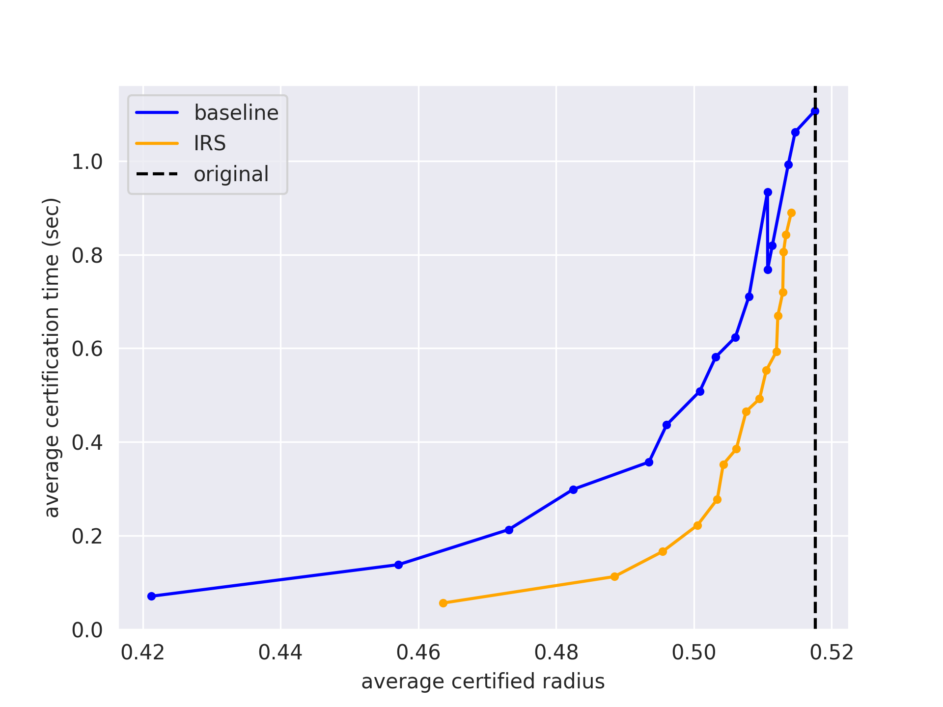
Figure 6: CIFAR10 ResNet-20 with $\sigma=1$, for $n_{p}\in\{5\%,10\%\dots 80\%\}$ of $n$

The objective of IRS is to certify the approximated DNN with few samples. Thus, we consider $n_{p}$ ranging from $1\%$ to $10\%$. Nevertheless, we check IRS effectiveness for larger $n_{p}$ values in this ablation study.

Since, IRS certifies radius $\sigma\Phi^{-1}(\underline{p_{A}}-\zeta_{x})$ that is always smaller than original certified radius. When $n_{p}=n$, the baseline running from scratch should perform better than IRS, as it will reach a certification radius close to $\sigma\Phi^{-1}(\underline{p_{A}})$.

In this experiment, on CIFAR10 ResNet-20 with $\sigma=1$, we let $n_{p}\in\{5\%,10\%\dots 80\%\}$ of $n$. Figure 6 shows the ACR vs mean time plot for the baseline and IRS. We see that IRS gives speedup for $n_{p}=70\%$. For $n_{p}=75\%$ and $n_{p}=80\%$, we see that baseline ACR is higher and IRS cannot achieve that ACR.

A.6 Threshold Parameter $\gamma$

Table 9 presents the proportion of cases for which $\underline{p_{A}}>\gamma$ for the $\gamma$ chosen through hyperparameter search in Section 5.3 for different $\sigma$ and networks.

Table 9: Proportion of $\underline{p_{A}}$ > $\gamma$ for different $\sigma$ and networks.

Dataset	Architecture	$\gamma$	$\sigma$	$\underline{p_{A}}>\gamma$
			0.25	0.346
CIFAR10	ResNet-20	0.99	0.5	0.162
			1.0	0.034
			0.25	0.362
CIFAR10	ResNet-110	0.99	0.5	0.146
			1.0	0.034
			0.5	0.292
ImageNet	ResNet-50	0.995	1.0	0.14
			2.0	0.04

For CIFAR10 ResNet-20, we observe that $\underline{p_{A}}>\gamma=0.346$ when $\sigma=0.25$ and $\underline{p_{A}}>\gamma=0.034$ when $\sigma=1.0$. Additionally, for ImageNet ResNet-50, the results show $\underline{p_{A}}>\gamma=0.292$ when $\sigma=0.50$ and $\underline{p_{A}}>\gamma=0.04$ when $\sigma=2.0$. As shown in Section 5, certifying larger $\sigma$ yields on average smaller $\underline{p_{A}}$. Expectedly, we see a smaller proportion of $\underline{p_{A}}>\gamma$ for larger $\sigma$ and vice versa.

A.7 Quantization Plots

In this section, we present the ACR vs time plots for all the quantization experiments.

(a) fp16

(b) bf16

(c) int8

Figure 7: ResNet-20 on CIFAR10 with $\sigma=0.25$.

(d) fp16

(e) bf16

(f) int8

Figure 8: ResNet-20 on CIFAR10 with $\sigma=0.5$.

(a) fp16

(b) bf16

(c) int8

Figure 9: ResNet-20 on CIFAR10 with $\sigma=1.0$.

(a) fp16

(b) bf16

(c) int8

Figure 10: ResNet-110 on CIFAR10 with $\sigma=0.25$.

(d) fp16

(e) bf16

(f) int8

Figure 11: ResNet-110 on CIFAR10 with $\sigma=0.5$.

(a) fp16

(b) bf16

(c) int8

Figure 12: ResNet-110 on CIFAR10 with $\sigma=1.0$.

(a) fp16

(b) bf16

(c) int8

Figure 13: ResNet-50 on ImageNet with $\sigma=0.5$.

(d) fp16

(e) bf16

(f) int8

Figure 14: ResNet-50 on ImageNet with $\sigma=1.0$.

(a) fp16

(b) bf16

(c) int8

Figure 15: ResNet-50 on ImageNet with $\sigma=2.0$.

References

- Agresti and Coull [1998] Alan Agresti and Brent A. Coull. Approximate is better than “exact” for interval estimation of binomial proportions. The American Statistician, 52(2):119–126, 1998. doi: 10.1080/00031305.1998.10480550. URL https://doi.org/10.1080/00031305.1998.10480550.
- Beyer et al. [2013] Dirk Beyer, Stefan Löwe, Evgeny Novikov, Andreas Stahlbauer, and Philipp Wendler. Precision reuse for efficient regression verification. In Proceedings of the 2013 9th Joint Meeting on Foundations of Software Engineering, ESEC/FSE 2013, page 389–399, New York, NY, USA, 2013. Association for Computing Machinery. ISBN 9781450322379. doi: 10.1145/2491411.2491429. URL https://doi.org/10.1145/2491411.2491429.
- Bojchevski et al. [2023] Aleksandar Bojchevski, Johannes Gasteiger, and Stephan Günnemann. Efficient robustness certificates for discrete data: Sparsity-aware randomized smoothing for graphs, images and more, 2023.
- Bunel et al. [2020] Rudy Bunel, Jingyue Lu, Ilker Turkaslan, Pushmeet Kohli, P Torr, and P Mudigonda. Branch and bound for piecewise linear neural network verification. Journal of Machine Learning Research, 21(2020), 2020.
- Clopper and Pearson [1934] C. J. Clopper and E. S. Pearson. The use of confidence or fiducial limits illustrated in the case of the binomial. Biometrika, 26(4):404–413, 1934. ISSN 00063444. URL http://www.jstor.org/stable/2331986.
- Cohen et al. [2019] Jeremy M. Cohen, Elan Rosenfeld, and J. Zico Kolter. Certified adversarial robustness via randomized smoothing. In Kamalika Chaudhuri and Ruslan Salakhutdinov, editors, Proceedings of the 36th International Conference on Machine Learning, ICML 2019, 9-15 June 2019, Long Beach, California, USA, volume 97 of Proceedings of Machine Learning Research, pages 1310–1320. PMLR, 2019. URL http://proceedings.mlr.press/v97/cohen19c.html.
- Deng et al. [2009] Jia Deng, Wei Dong, Richard Socher, Li-Jia Li, Kai Li, and Li Fei-Fei. Imagenet: A large-scale hierarchical image database. In 2009 IEEE conference on computer vision and pattern recognition, pages 248–255. Ieee, 2009.
- Dvijotham et al. [2020] Krishnamurthy (Dj) Dvijotham, Jamie Hayes, Borja Balle, Zico Kolter, Chongli Qin, Andras Gyorgy, Kai Xiao, Sven Gowal, and Pushmeet Kohli. A framework for robustness certification of smoothed classifiers using f-divergences. In International Conference on Learning Representations, 2020. URL https://openreview.net/forum?id=SJlKrkSFPH.
- Fischer et al. [2020] Marc Fischer, Maximilian Baader, and Martin Vechev. Certified defense to image transformations via randomized smoothing. In H. Larochelle, M. Ranzato, R. Hadsell, M.F. Balcan, and H. Lin, editors, Advances in Neural Information Processing Systems, volume 33, pages 8404–8417. Curran Associates, Inc., 2020. URL https://proceedings.neurips.cc/paper_files/paper/2020/file/5fb37d5bbdbbae16dea2f3104d7f9439-Paper.pdf.
- Fischer et al. [2022a] Marc Fischer, Maximilian Baader, and Martin Vechev. Scalable certified segmentation via randomized smoothing, 2022a.
- Fischer et al. [2022b] Marc Fischer, Christian Sprecher, Dimitar I. Dimitrov, Gagandeep Singh, and Martin T. Vechev. Shared certificates for neural network verification. In Sharon Shoham and Yakir Vizel, editors, Computer Aided Verification - 34th International Conference, CAV 2022, Haifa, Israel, August 7-10, 2022, Proceedings, Part I, volume 13371 of Lecture Notes in Computer Science, pages 127–148. Springer, 2022b. doi: 10.1007/978-3-031-13185-1\_7. URL https://doi.org/10.1007/978-3-031-13185-1_7.
- Frankle and Carbin [2019] Jonathan Frankle and Michael Carbin. The lottery ticket hypothesis: Finding sparse, trainable neural networks. In Proc. International Conference on Learning Representations (ICLR), 2019.
- Gao et al. [2020] Zhidong Gao, Rui Hu, and Yanmin Gong. Certified robustness of graph classification against topology attack with randomized smoothing. In GLOBECOM 2020 - 2020 IEEE Global Communications Conference, pages 1–6, 2020. doi: 10.1109/GLOBECOM42002.2020.9322576.
- Horváth et al. [2022] Miklós Z. Horváth, Mark Niklas Mueller, Marc Fischer, and Martin Vechev. Boosting randomized smoothing with variance reduced classifiers. In International Conference on Learning Representations, 2022. URL https://openreview.net/forum?id=mHu2vIds_-b.
- Jia et al. [2020] Jinyuan Jia, Xiaoyu Cao, Binghui Wang, and Neil Zhenqiang Gong. Certified robustness for top-k predictions against adversarial perturbations via randomized smoothing. In International Conference on Learning Representations, 2020. URL https://openreview.net/forum?id=BkeWw6VFwr.
- Johnson et al. [2013] Kenneth Johnson, Radu Calinescu, and Shinji Kikuchi. An incremental verification framework for component-based software systems. In Proceedings of the 16th International ACM Sigsoft Symposium on Component-Based Software Engineering, CBSE ’13, page 33–42, New York, NY, USA, 2013. Association for Computing Machinery. ISBN 9781450321228. doi: 10.1145/2465449.2465456. URL https://doi.org/10.1145/2465449.2465456.
- Katz et al. [2017] Guy Katz, Clark W. Barrett, David L. Dill, Kyle Julian, and Mykel J. Kochenderfer. Reluplex: An efficient SMT solver for verifying deep neural networks. In Computer Aided Verification - 29th International Conference, CAV 2017, Heidelberg, Germany, July 24-28, 2017, Proceedings, Part I, volume 10426 of Lecture Notes in Computer Science, 2017. doi: 10.1007/978-3-319-63387-9\_5.
- [18] Alex Krizhevsky, Vinod Nair, and Geoffrey Hinton. Cifar-10 (canadian institute for advanced research). URL http://www.cs.toronto.edu/~kriz/cifar.html.
- Kumar et al. [2020] Aounon Kumar, Alexander Levine, Soheil Feizi, and Tom Goldstein. Certifying confidence via randomized smoothing. In H. Larochelle, M. Ranzato, R. Hadsell, M.F. Balcan, and H. Lin, editors, Advances in Neural Information Processing Systems, volume 33, pages 5165–5177. Curran Associates, Inc., 2020. URL https://proceedings.neurips.cc/paper_files/paper/2020/file/37aa5dfc44dddd0d19d4311e2c7a0240-Paper.pdf.
- Lakhnech et al. [2001] Yassine Lakhnech, Saddek Bensalem, Sergey Berezin, and Sam Owre. Incremental verification by abstraction. In T. Margaria and W. Yi, editors, Tools and Algorithms for the Construction and Analysis of Systems: 7th International Conference, TACAS 2001, volume 2031, pages 98–112, Genova, Italy, April 2001. Springer-Verlag.
- Laurel et al. [2021] Jacob Laurel, Rem Yang, Atharva Sehgal, Shubham Ugare, and Sasa Misailovic. Statheros: Compiler for efficient low-precision probabilistic programming. In 2021 58th ACM/IEEE Design Automation Conference (DAC), pages 787–792, 2021. doi: 10.1109/DAC18074.2021.9586276.
- Laurel et al. [2022] Jacob Laurel, Rem Yang, Shubham Ugare, Robert Nagel, Gagandeep Singh, and Sasa Misailovic. A general construction for abstract interpretation of higher-order automatic differentiation. Proc. ACM Program. Lang., 6(OOPSLA2), oct 2022. doi: 10.1145/3563324. URL https://doi.org/10.1145/3563324.
- Lee et al. [2019] Guang-He Lee, Yang Yuan, Shiyu Chang, and Tommi Jaakkola. Tight certificates of adversarial robustness for randomly smoothed classifiers. In H. Wallach, H. Larochelle, A. Beygelzimer, F. d'Alché-Buc, E. Fox, and R. Garnett, editors, Advances in Neural Information Processing Systems, volume 32. Curran Associates, Inc., 2019. URL https://proceedings.neurips.cc/paper_files/paper/2019/file/fa2e8c4385712f9a1d24c363a2cbe5b8-Paper.pdf.
- Levine and Feizi [2020] Alexander Levine and Soheil Feizi. (de)randomized smoothing for certifiable defense against patch attacks. In Hugo Larochelle, Marc’Aurelio Ranzato, Raia Hadsell, Maria-Florina Balcan, and Hsuan-Tien Lin, editors, Advances in Neural Information Processing Systems 33: Annual Conference on Neural Information Processing Systems 2020, NeurIPS 2020, December 6-12, 2020, virtual, 2020. URL https://proceedings.neurips.cc/paper/2020/hash/47ce0875420b2dbacfc5535f94e68433-Abstract.html.
- Li et al. [2021] Linyi Li, Maurice Weber, Xiaojun Xu, Luka Rimanic, Bhavya Kailkhura, Tao Xie, Ce Zhang, and Bo Li. Tss: Transformation-specific smoothing for robustness certification. In Proceedings of the 2021 ACM SIGSAC Conference on Computer and Communications Security, CCS ’21, page 535–557, New York, NY, USA, 2021. Association for Computing Machinery. ISBN 9781450384544. doi: 10.1145/3460120.3485258. URL https://doi.org/10.1145/3460120.3485258.
- Lin et al. [2021] Haowen Lin, Jian Lou, Li Xiong, and Cyrus Shahabi. Integer-arithmetic-only certified robustness for quantized neural networks. In 2021 IEEE/CVF International Conference on Computer Vision, ICCV 2021, Montreal, QC, Canada, October 10-17, 2021, pages 7808–7817. IEEE, 2021. doi: 10.1109/ICCV48922.2021.00773. URL https://doi.org/10.1109/ICCV48922.2021.00773.
- Liu et al. [2021] Hongbin Liu, Jinyuan Jia, and Neil Zhenqiang Gong. Pointguard: Provably robust 3d point cloud classification, 2021.
- Mohapatra et al. [2020] Jeet Mohapatra, Ching-Yun Ko, Tsui-Wei Weng, Pin-Yu Chen, Sijia Liu, and Luca Daniel. Higher-order certification for randomized smoothing, 2020.
- Mohapatra et al. [2021] Jeet Mohapatra, Ching-Yun Ko, Lily Weng, Pin-Yu Chen, Sijia Liu, and Luca Daniel. Hidden cost of randomized smoothing. In Arindam Banerjee and Kenji Fukumizu, editors, Proceedings of The 24th International Conference on Artificial Intelligence and Statistics, volume 130 of Proceedings of Machine Learning Research, pages 4033–4041. PMLR, 13–15 Apr 2021. URL https://proceedings.mlr.press/v130/mohapatra21a.html.
- O’Hearn [2018] Peter W. O’Hearn. Continuous reasoning: Scaling the impact of formal methods. In Anuj Dawar and Erich Grädel, editors, Proceedings of the 33rd Annual ACM/IEEE Symposium on Logic in Computer Science, LICS 2018, Oxford, UK, July 09-12, 2018, pages 13–25. ACM, 2018. doi: 10.1145/3209108.3209109. URL https://doi.org/10.1145/3209108.3209109.
- Paszke et al. [2019] Adam Paszke, Sam Gross, Francisco Massa, Adam Lerer, James Bradbury, Gregory Chanan, Trevor Killeen, Zeming Lin, Natalia Gimelshein, Luca Antiga, Alban Desmaison, Andreas Kopf, Edward Yang, Zachary DeVito, Martin Raison, Alykhan Tejani, Sasank Chilamkurthy, Benoit Steiner, Lu Fang, Junjie Bai, and Soumith Chintala. Pytorch: An imperative style, high-performance deep learning library. In Advances in Neural Information Processing Systems 32, pages 8024–8035. Curran Associates, Inc., 2019. URL http://papers.neurips.cc/paper/9015-pytorch-an-imperative-style-high-performance-deep-learning-library.pdf.
- Rosenfeld et al. [2020] Elan Rosenfeld, Ezra Winston, Pradeep Ravikumar, and J. Zico Kolter. Certified robustness to label-flipping attacks via randomized smoothing, 2020.
- Schuchardt et al. [2021] Jan Schuchardt, Aleksandar Bojchevski, Johannes Gasteiger, and Stephan Günnemann. Collective robustness certificates: Exploiting interdependence in graph neural networks. In International Conference on Learning Representations, 2021. URL https://openreview.net/forum?id=ULQdiUTHe3y.
- Sehwag et al. [2020] Vikash Sehwag, Shiqi Wang, Prateek Mittal, and Suman Jana. Hydra: Pruning adversarially robust neural networks, 2020.
- Stein et al. [2021] Benno Stein, Bor-Yuh Evan Chang, and Manu Sridharan. Demanded abstract interpretation. In Stephen N. Freund and Eran Yahav, editors, PLDI ’21: 42nd ACM SIGPLAN International Conference on Programming Language Design and Implementation, Virtual Event, Canada, June 20-25, 2021, pages 282–295. ACM, 2021. doi: 10.1145/3453483.3454044. URL https://doi.org/10.1145/3453483.3454044.
- Tjeng et al. [2017] Vincent Tjeng, Kai Xiao, and Russ Tedrake. Evaluating robustness of neural networks with mixed integer programming. arXiv preprint arXiv:1711.07356, 2017.
- Ugare et al. [2022] Shubham Ugare, Gagandeep Singh, and Sasa Misailovic. Proof transfer for fast certification of multiple approximate neural networks. Proc. ACM Program. Lang., 6(OOPSLA):1–29, 2022. doi: 10.1145/3527319. URL https://doi.org/10.1145/3527319.
- Ugare et al. [2023] Shubham Ugare, Debangshu Banerjee, Sasa Misailovic, and Gagandeep Singh. Incremental verification of neural networks, 2023.
- Visser et al. [2012] Willem Visser, Jaco Geldenhuys, and Matthew B. Dwyer. Green: Reducing, reusing and recycling constraints in program analysis. In Proceedings of the ACM SIGSOFT 20th International Symposium on the Foundations of Software Engineering, FSE ’12, New York, NY, USA, 2012. Association for Computing Machinery. ISBN 9781450316149. doi: 10.1145/2393596.2393665. URL https://doi.org/10.1145/2393596.2393665.
- Voracek and Hein [2023] Vaclav Voracek and Matthias Hein. Sound randomized smoothing in floating-point arithmetic. In The Eleventh International Conference on Learning Representations, 2023. URL https://openreview.net/forum?id=HaHCoGcpV9.
- Wang et al. [2021a] Binghui Wang, Jinyuan Jia, Xiaoyu Cao, and Neil Zhenqiang Gong. Certified robustness of graph neural networks against adversarial structural perturbation. In Proceedings of the 27th ACM SIGKDD Conference on Knowledge Discovery & Data Mining, KDD ’21, page 1645–1653, New York, NY, USA, 2021a. Association for Computing Machinery. ISBN 9781450383325. doi: 10.1145/3447548.3467295. URL https://doi.org/10.1145/3447548.3467295.
- Wang et al. [2021b] Shiqi Wang, Huan Zhang, Kaidi Xu, Xue Lin, Suman Jana, Cho-Jui Hsieh, and J Zico Kolter. Beta-crown: Efficient bound propagation with per-neuron split constraints for complete and incomplete neural network verification. arXiv preprint arXiv:2103.06624, 2021b.
- Wei and Liu [2021] Tianhao Wei and Changliu Liu. Online verification of deep neural networks under domain or weight shift. CoRR, abs/2106.12732, 2021. URL https://arxiv.org/abs/2106.12732.
- Wilson [1927] Edwin B. Wilson. Probable inference, the law of succession, and statistical inference. Journal of the American Statistical Association, 22(158):209–212, 1927. ISSN 01621459. URL http://www.jstor.org/stable/2276774.
- Yang et al. [2020] Greg Yang, Tony Duan, J. Edward Hu, Hadi Salman, Ilya Razenshteyn, and Jerry Li. Randomized smoothing of all shapes and sizes, 2020.
- Yang et al. [2009] Guowei Yang, Matthew B. Dwyer, and Gregg Rothermel. Regression model checking. In 2009 IEEE International Conference on Software Maintenance, pages 115–124, 2009. doi: 10.1109/ICSM.2009.5306334.
- yeh Chiang et al. [2022] Ping yeh Chiang, Michael J. Curry, Ahmed Abdelkader, Aounon Kumar, John Dickerson, and Tom Goldstein. Detection as regression: Certified object detection by median smoothing, 2022.
- Zhang et al. [2020] Dinghuai Zhang, Mao Ye, Chengyue Gong, Zhanxing Zhu, and Qiang Liu. Black-box certification with randomized smoothing: A functional optimization based framework. In H. Larochelle, M. Ranzato, R. Hadsell, M.F. Balcan, and H. Lin, editors, Advances in Neural Information Processing Systems, volume 33, pages 2316–2326. Curran Associates, Inc., 2020. URL https://proceedings.neurips.cc/paper_files/paper/2020/file/1896a3bf730516dd643ba67b4c447d36-Paper.pdf.
- Zhou et al. [2017] Aojun Zhou, Anbang Yao, Yiwen Guo, Lin Xu, and Yurong Chen. Incremental network quantization: Towards lossless CNNs with low-precision weights. In International Conference on Learning Representations, 2017. URL https://openreview.net/forum?id=HyQJ-mclg.