Stabilization of stochastic nonlinear systems via double-event-triggering mechanisms and switching controls

Abstract

In this paper, we concentrate on the exponential stabilization of stochastic nonlinear systems. Different from the single event-triggering mechanism in traditional deterministic/stochastic control systems, based on two stopping time sequences, we put forward a double-event-triggering mechanism (DETM) to update control signals and make two different controls switch in order. Also, this novel DETM allows aperiodic time updating and guarantees a positive lower bound on the inter-event times. Together with this DETM, we introduce a switching control law, including a primary control and a secondary control for a non-switched stochastic system to obtain the exponential stabilization and boundedness results. Finally, an illustrative example with simulation figures is given to demonstrate the obtained results.

1 Introduction

In the passing decades, stability and control problems of stochastic nonlinear systems have attracted widespread attention in engineering, neural networks, physics and so on. Nowadays, a large number of control functions are available for stochastic and deterministic systems, like continuous controls, sampled-data controls, intermittent controls, switching controls and so on (see, e.g., [1, 2, 3, 4, 5, 6, 7, 8, 9, 10, 11, 12]). In consideration of control cost, sampled-data controls and intermittent controls are great options. For example, in [10], the authors put forward a periodically intermittent control

$$u(t)=\left\{\begin{array}[]{l}Kx(t),~{}nT\leq t<nT+\tau,\\ 0,~{}~{}~{}~{}~{}nT+\tau\leq t<(n+1)T,\end{array}\right.$$

where $K$ is the control gain matrix, $T$ is the control period and $\tau$ is the control width. With the development of intermittent controls (see, e.g., [11, 12]), periodically intermittent controls are gradually being replaced by aperiodic intermittent controls, such as

$$u(t)=\left\{\begin{array}[]{l}Kx(t),~{}t_{i}\leq t<t_{i}+\tau,\\ 0,~{}~{}~{}~{}~{}~{}~{}t_{i}+\tau\leq t<t_{i+1},\end{array}\right.$$

where $t_{i+1}-t_{i}\not\equiv T$. Recently, Liu et al. in [13] have applied an important sampling technique called event-triggering mechanism (ETM) to intermittent controls and proposed an aperiodic event-triggered intermittent control as follows:

$$u(t)=\left\{\begin{array}[]{l}Kx(t),~{}t_{i}\leq t<t_{i}+\tau_{i},\\ 0,~{}~{}~{}~{}~{}~{}~{}t_{i}+\tau_{i}\leq t<t_{i+1},\end{array}\right.$$ (3)

where $t_{i}$ is updated by ETM. Compared to the traditional time-triggering mechanism, ETM provides aperiodic implementations according to the triggering conditions. The time will be updated only when triggering conditions are met. Hence, ETM can reduce redundant data transmission and efficiently save the network communication resources. However, in (3), $\tau_{i}$ is not updated by ETM. Although $\tau_{i}$ may not be a constant, the choice of $\tau_{i}$ is difficult under some restrictive conditions like (41) and (42) in [13], such that in the numerical example, the authors in [13] took $\tau_{i}\equiv\tau=1.5$. Then it is natural to ask whether $\tau_{i}$ can be updated by ETM? In real life, for example, the light sensing lamps will turn off when they sense strong sunlight and turn on when the sunlight is weak. Hence, it is more interesting and challenging to investigate a novel ETM which can generate two time sequences for control updating and switching.

Motivated by the above discussion, we put forward the following double-ETM (DETM):

$$s_{i}=\inf\{t>t_{i}\big{|}~{}\Psi_{1}(t,t_{i})\geq 0\},$$

$$t_{i+1}=\inf\{t>s_{i}\big{|}~{}\Psi_{2}(t,s_{i})\geq 0\},$$ (4)

where $\Psi_{1}(t,t_{i})$ and $\Psi_{2}(t,s_{i})$ are two events based on the system state $x(\cdot)$. DETM (4) can determine two execution time sequences $\{t_{i}\}$, $\{s_{i}\}$ and they alternate in all stages, i.e., $[0,+\infty)=[t_{0},s_{0})\cup[s_{0},t_{1})\cup[t_{1},s_{1})\ldots$ with $t_{0}=0$. As a simple example, we consider the state function $x=\frac{e\sin 3t}{t}+2,~{}t>0$ and use the following DETM:

$$s_{i}=\inf\{t>t_{i}~{}\big{|}~{}x\leq M_{2}\},$$

$$t_{i+1}=\inf\{t>s_{i}~{}\big{|}~{}x\geq M_{1}\},$$ (5)

where $i=0,1,\ldots$ and $t_{0}=0$ (see Fig 1).

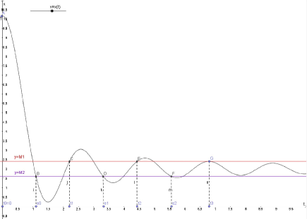
Figure 1: Configuration of DETM.

As we know, the classical switching controls are proposed for switched systems (see, e.g., [14, 15, 16, 17, 18, 19]). For instance, a switched system $\dot{x}(t)=f_{\sigma(t)}(x_{t},u(t))$ is considered in [19] and the control $u(t)$ switches according to the switching signal $\sigma(t)$. But in this paper, based on DETM (4), we construct a novel switching control $u(t)$, including a primary control $u_{1}(t)$ and a secondary control $u_{2}(t)$ for a non-switched system as follows:

$$u(t)=\left\{\begin{array}[]{l}u_{1}(t),~{}~{}t\in[t_{i},s_{i}),\\ u_{2}(t),~{}~{}t\in[s_{i},t_{i+1}),\end{array}\right.$$ (8)

where the switching time sequences $\{t_{i}\}$ and $\{s_{i}\}$ are both induced by DETM. Two controls $u_{1}$ and $u_{2}$ switch in order according to $\{t_{i}\}$ and $\{s_{i}\}$. Especially, if $u_{1}\neq 0$ and $u_{2}=0$, then the switching control $u(t)$ degenerates into the intermittent control. Since most existing results on ETMs are available for deterministic control systems (see, e.g., [20, 21, 22, 23, 24]), we will face many challenges and obstacles when applying this switching control and DETM to stochastic systems. This is because for stochastic systems, triggering conditions $\Psi_{1}(t,t_{i})$ and $\Psi_{2}(t,s_{i})$ rely on the stochastic process $x(t)$ such that $\{t_{i}\}$ and $\{s_{i}\}$ are two sequences of stopping times, which will cause a lot of difficulties when considering the stabilization problem and the Zeno phenomenon. Moreover, although there are a few results on stochastic control systems (see, e.g., [25, 26, 27, 28, 29, 30, 31]), event-triggered controls (ETCs) presented above are all based on a single ETM and some restrictions are given to avoid the Zeno phenomenon. Hence, to realize the stabilization of stochastic systems and reduce the restrictive conditions for time regularization at the same time, the design of switching control and DETM requires many stochastic analysis techniques and the consideration of some new difficulties.

Consequently, in this paper, we present a switching control law based on a novel DETM to ensure a desirable stabilization of stochastic nonlinear systems. To the best of our knowledge, our paper is the first to put forward this DETM for stochastic control systems and it is novel even in the deterministic control systems. Compared to the traditional works, the main contributions of the proposed methods are summarized as follows:

(1) For a non-switched stochastic system, a novel switching control is established, which admits two different controls $u_{1}$ and $u_{2}$. It is more flexible for stabilization of stochastic systems because we can construct $u_{1}$ and $u_{2}$, respectively. Namely, we can choose continuous/discrete controllers to stabilize systems or choose two controls with opposite effects, like countermeasure controls. Especially, if $u_{1}\neq 0$ and $u_{2}=0$, then this switching control degenerates into an intermittent control, generalizing those periodic and aperiodic intermittent controls in [10, 11, 12, 13].

(2) Different from the traditional sampled-data controls based on time-triggering mechanisms (see, e.g., [3, 4, 7, 8]), in this paper, the switching signal and control updating time are induced by DETM, which can reduce redundant data transmission and efficiently save the network communication resources. Also, compared to those event-triggered controls dependent on one single ETM (see, e.g., [25, 30, 31]), DETM can not only solve the Zeno phenomenon more effectively, but also reduce the restrictive conditions for time regularization.

The rest of this paper is organized as follows. In Section 2, we present the notations and introduce the model with an Itô operator. In Section 3, we propose a detailed design of DETM with execution rules and a novel switching control law based on DETM. Then, the switching control with different execution rules is applied to guarantee the mean square exponential stabilization and boundedness of stochastic nonlinear systems in Section 4 and Section 5, respectively. For illustration of the obtained results, an example on the pitch motion of a symmetric satellite is provided with simulation figures in Section 6. Finally, the conclusion and future research prospects are given in the last section.

2 Preliminaries

2.1 Notations

In this paper, we use the following notations. $\mathbf{N}=\{0,1,2,\ldots\}$, $\mathbf{R}=(-\infty,\infty)$ and $\mathbf{R}^{+}=[0,\infty)$. For two positive integers $n$ and $m$, $\mathbf{R}^{n}$ denotes the set of real vectors with the Euclidean norm $|\cdot|$ and $\mathbf{R}^{n\times m}$ denotes the set of real matrices with the induced Euclidean norm $\|\cdot\|$. Let $\mathbf{C}^{i}(\mathbf{R}^{n};\mathbf{R}^{+})$, $i=0,1,2$ stand for the space of the continuous functions from $\mathbf{R}^{n}$ to $\mathbf{R}^{+}$ with $i$-th order continuous (partial) derivatives. Moreover, $\alpha\wedge\beta=\min\{\alpha,\beta\}$ and $\alpha\vee\beta=\max\{\alpha,\beta\}$.

Let $(\Omega,{\mathcal{F}},\{{\mathcal{F}}_{t}\}_{t\geq 0},P)$ be a complete probability space with a natural filtration $\{{\mathcal{F}}_{t}\}_{t\geq 0}$ satisfying the usual conditions, i.e., $\{{\mathcal{F}}_{t}\}_{t\geq 0}$ is right continuous and ${\mathcal{F}}_{0}$ contains all $P$-null sets. $W(t)=(W_{1}(t),W_{2}(t),\ldots,W_{m}(t))^{T},~{}t\geq 0$ is an $m$-dimensional standard Wiener process adapted to the filtration $\{{\mathcal{F}}_{t}\}_{t\geq 0}$ on $(\Omega,{\mathcal{F}},\{{\mathcal{F}}_{t}\}_{t\geq 0},P)$.

2.2 Model description

Consider the following stochastic nonlinear system:

$$\left\{\begin{array}[]{l}dx(t)=f(x(t),u(t))dt+g(x(t))dW(t),~{}~{}t>0,\\ x(0)=\phi,\end{array}\right.$$ (9)

where $x\in\mathbf{R}^{n}$, $u\in\mathbf{U}\subset\mathbf{R}^{l}$ is a control input and $\mathbf{U}$ is a compact set with $0\in\mathbf{U}$. $f(\cdot,\cdot):\mathbf{R}^{n}\times\mathbf{R}^{l}\rightarrow\mathbf{R}^{n}$ and $g(\cdot):\mathbf{R}^{n}\rightarrow\mathbf{R}^{n\times m}$ are both continuous functions satisfying the local Lipschitz condition with $f(0,0)=0$ and $g(0)=0$. Then it follows from [25] that system $(\ref{301})$ admits a unique global solution.

For a function $V\in\mathbf{C}^{2}(\mathbf{R}^{n};\mathbf{R}^{+})$, we present the Itô operator for system (9):

$$\mathcal{L}V(x,u)=\frac{\partial V}{\partial x}f(x,u)+\frac{1}{2}trace(g^{T}(x)\frac{\partial^{2}V}{\partial x^{2}}g(x)),$$

where $\frac{\partial V}{\partial x}=\Big{(}\frac{\partial V(x)}{\partial x_{1}},\frac{\partial V(x)}{\partial x_{2}},\ldots,\frac{\partial V(x)}{\partial x_{n}}\Big{)}$ and $\frac{\partial^{2}V}{\partial x^{2}}=\Big{(}\frac{\partial^{2}V(x)}{\partial x_{i}\partial x_{j}}\Big{)}_{n\times n}$.

3 Switching control based on DETM

In this section, we introduce a detailed design of DETM with execution rules and present a switching control law based on DETM.

DETM: the execution rule. Let $h_{1}(t),~{}h_{2}(t):\mathbf{R}^{+}\rightarrow\mathbf{R}^{+}$ be two adjustable functions. Given a positive constant $\tau$, if the initial value ${|x(0)|^{2}\leq h_{2}(0)}$, then we use the following rules:

$$t_{i}=\inf\{t>s_{i}~{}\big{|}~{}{|x(t)|^{2}}\geq h_{1}(t)\},$$

$$s_{i+1}=\inf\{t>t_{i}+\tau~{}\big{|}~{}{|x(t)|^{2}}\leq h_{2}(t)\},$$ (10)

$i=0,1,\ldots$ with $s_{0}=0$.

If the initial value ${|x(0)|^{2}>h_{2}(0)}$, then we use the following rules:

$$s_{i}=\inf\{t>t_{i}+\tau~{}\big{|}~{}{|x(t)|^{2}}\leq h_{2}(t)\},$$ (11)

$$t_{i+1}=\inf\{t>s_{i}~{}\big{|}~{}{|x(t)|^{2}}\geq h_{1}(t)\},$$ (12)

$i=0,1,\ldots$ with $t_{0}=0$.

Without loss of generality, we consider ${|x(0)|^{2}>h_{2}(0)}$ in this paper.

Switching control. Based on the time sequences $\{t_{i}\}_{i\in\mathbf{N}}$ and $\{s_{i}\}_{i\in\mathbf{N}}$ induced by execution rules (11)-(12), the switching control is designed as:

$$u(t)=\left\{\begin{array}[]{l}u_{1}(t)=k_{1}(x(t)),~{}~{}t\in[t_{i},s_{i}),\\ u_{2}(t)=k_{2}(x(t)),~{}~{}t\in[s_{i},t_{i+1}),\end{array}\right.$$ (15)

where $k_{i}:\mathbf{R}^{n}\rightarrow\mathbf{R}^{l}$, $i=1,2$ satisfy $k_{i}(0)=0$ and the local Lipschitz condition. At each time instant $t_{i}$ or $s_{i}$, the primary control $u_{1}(t)$ and the secondary control $u_{2}(t)$ exchange with each other. While between consecutive control updates, the control $u(t)$ stays unchanged.

Remark 1.

Similar to [25, 32, 33], we use a time regularization $\tau$ to avoid the Zeno phenomenon. But there is no need to add $\tau$ in both ETM (11) and ETM (12). Only one triggering condition needs a positive constant $\tau$. Namely, under ETM (11), if execution occurs and the triggering time $t$ is less than $t_{i}+\tau$, then the primary control $u_{1}(t)$ will remain working for a fixed period of time (i.e., $s_{i}=t_{i}+\tau$). Otherwise, the triggering time $s_{i}=t$. Hence, the length of each interval $t_{i+1}-t_{i}=(t_{i+1}-s_{i})+(s_{i}-t_{i})$ is clearly not less than $\tau$, which means that the Zeno phenomenon or even, infinitely fast execution/sampling cannot occur. Then it is natural to ask which condition to add this time regularization $\tau$, ETM (11) or ETM (12)? A prominent advantage of our DETM is that the time regularization $\tau$ is added in ETM (11) rather than ETM (12), which can avoid the Zeno phenomenon and at the same time, reduce the restrictive conditions on $\tau$ in [25, 32, 33]. The specific reason will be discussed later in Remark 4.

Remark 2.

Compared to the traditional single ETM in [25, 28, 30, 31], the switching control law (15) based on DETM admits two different controls $u_{1}$ and $u_{2}$ such that it has more flexibility for control design of stochastic systems. If one of the controls equals 0, then the switching control degenerates into the aperiodic intermittent control. Also, switching signals $\{t_{i}\}$ and $\{s_{i}\}$ in (15) are both induced by ETMs and they are in nature stochastic (i.e., stopping times), which generate those intermittent controls in [10, 12, 13].

The configuration of DETM and switching control is given by the following procedure (see Fig 2):

Step 1: When $t$ starts from $t_{i}$, we apply the primary control $u(t)=u_{1}(t)$;

Step 2: According to DETM (11), we obtain the triggering time $t=s_{i}$ and change the control input, i.e., use the secondary control $u(t)=u_{2}(t)$ from $t=s_{i}$ until the next triggering time;

Step 3: Update $t_{i}$. Based on DETM (12), we obtain $t_{i+1}$ and go into step 1 for $t=t_{i+1}$.

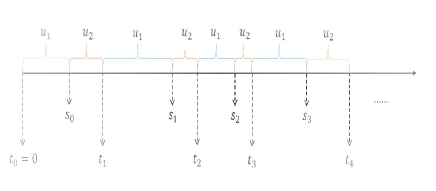
Figure 2: Configuration of switching control based on DETM.

4 Exponential stabilization of stochastic systems

In this section, we present the specific expressions for functions $h_{1}(t)$ and $h_{2}(t)$ in the execution rule. Also, under three key assumptions, the exponential stabilization is considered for system $(\ref{301})$.

In DETM (11)-(12), take $h_{1}(t)=M_{1}e^{-\lambda t}$ and $h_{2}(t)=M_{2}e^{-\lambda t}$, i.e.,

$$s_{i}=\inf\{t>t_{i}+\tau~{}\big{|}~{}|x(t)|^{2}\leq M_{2}e^{-\lambda t}\},$$ (16)

$$t_{i+1}=\inf\{t>s_{i}~{}\big{|}~{}|x(t)|^{2}\geq M_{1}e^{-\lambda t}\},$$ (17)

where constants $\lambda>0$, $0<M_{2}\leq M_{1}$ and $M_{2}<|x(0)|^{2}$.

Remark 3.

There are some different constructions of DETM (16)-(17). For example, $\lambda$ in ETM (16) and ETM (17) can be different, i.e.,

$$s_{i}=\inf\{t>t_{i}+\tau~{}\big{|}~{}|x(t)|^{2}\leq M_{1}e^{-\lambda_{2}t}\},$$

$$t_{i+1}=\inf\{t>s_{i}~{}\big{|}~{}|x(t)|^{2}\geq M_{2}e^{-\lambda_{1}t}\},$$

with $\lambda_{1}>\lambda_{2}$. Also, DETM can be designed as

$$s_{i}=\inf\{t>t_{i}+\tau~{}\big{|}~{}|x(t)|^{2}\leq M_{2}e^{-\lambda_{1}t}\},$$

$$t_{i+1}=\inf\{t>s_{i}~{}\big{|}~{}|x(t)|^{2}\geq M_{1}e^{-\lambda_{2}t}+\delta(t)\},$$

where $\delta(t)$ is an adjustable function satisfying $\lim\limits_{t\rightarrow+\infty}\delta(t)=0$. Then $\delta(t)$ can be chosen very large in the initial period to reduce the working time of the primary control and increase economic efficiency.

${\bf Assumption\ 1}$. There exists a function $V\in\mathbf{C}^{2}(\mathbf{R}^{n};\mathbf{R}^{+})$ satisfying $c_{1}|x|^{2}\leq V(x)\leq c_{2}|x|^{2}$, where constants $c_{1},c_{2}>0$.

${\bf Assumption\ 2}$. There exist two local Lipschitz mappings $k_{1}:\mathbf{R}^{n}\rightarrow\mathbf{U}$ with $k_{1}(0)=0$ and $k_{2}:\mathbf{R}^{n}\rightarrow\mathbf{U}$ with $k_{2}(0)=0$. Moreover, the following inequalities hold:

$$\mathcal{L}V(x,k_{1}(x))\leq-\mu|x|^{2}+\bar{M}e^{-\bar{\lambda}t},$$ (18)

$$\mathcal{L}V(x,k_{2}(x))\leq c_{3}|x|^{2},$$ (19)

where constants $\mu>0$, $\bar{M}\geq 0$, $\bar{\lambda}<\frac{\mu}{c_{2}}$ and $c_{3}\in\mathbf{R}$.

Remark 4.

Inequality (18) is a classical stable condition while inequality (19) is weaker since $c_{3}$ can be nonnegative. Also, it is worth mentioning that, based on inequality (18), the system will become more stable if time regularization $\tau$ in ETM (16) becomes larger. This is because the primary control $k_{1}$ holds on $[t_{i},s_{i})$ and $s_{i}-t_{i}\geq\tau$. Hence, there is no restrictive condition on the upper bound of $\tau$ and it is the biggest difference from those traditional ETMs in [25, 32, 33]. If $\tau$ is added in ETM (17), then we need similar restrictive conditions on $\tau$ in [25, 32, 33] because the secondary control $k_{2}$ may play a negative role in the stabilization. By the way, from the cost of controls, the less time $k_{1}$ works, the better. Then, one can choose a sufficiently small $\tau$ as long as it can avoid the Zeno phenomenon.

Remark 5.

Under the conditions (18)-(19) in Assumption 2, it can be seen that in DETM (16)-(17), if $M_{2}$ is chosen smaller, then the primary control $k_{1}$ works longer and if $M_{1}$ is chosen larger, then the secondary control $k_{2}$ works longer.

${\bf Assumption\ 3}$. $\lambda$ in DETM (16)-(17) satisfies $\lambda<\bar{\lambda}<\frac{\mu}{c_{2}}$ for $\bar{M}>0$ and $\lambda<\frac{\mu}{c_{2}}$ for $\bar{M}=0$.

Remark 6.

Assumption 3 is given to guarantee the existence of $s_{i}$ in ETM (16). Under Assumption 3, if $\bar{M}>0$, choose a positive constant $\gamma$ such that $\bar{\lambda}<\gamma<\frac{\mu}{c_{2}}$. Then for $t_{i}\leq t<s_{i}$, we have

$$\mathbf{E}[e^{\gamma t}V(x(t))-e^{\gamma t_{i}}V(x(t_{i}))|{\mathcal{F}}_{t_{i}}]$$

$$\leq\int_{t_{i}}^{t}\mathbf{E}[\gamma e^{\gamma s}V(x(s))+e^{\gamma s}\mathcal{L}V(x(s),k_{1}(x(s)))|{\mathcal{F}}_{t_{i}}]ds$$

$$\leq c_{2}\gamma\int_{t_{i}}^{t}e^{\gamma s}\mathbf{E}[|x(s)|^{2}|{\mathcal{F}}_{t_{i}}]ds+\int_{t_{i}}^{t}e^{\gamma s}(-\mu\mathbf{E}[|x(s)|^{2}|{\mathcal{F}}_{t_{i}}]+\bar{M}e^{-\bar{\lambda}s})ds$$ (20)

$$\leq\frac{\bar{M}}{\gamma-\bar{\lambda}}e^{(\gamma-\bar{\lambda})t}.$$ (21)

Taking mathematical expectation on both sides of (21) to obtain

$$e^{\gamma t}\mathbf{E}V(x(t))-e^{\gamma t_{i}}\mathbf{E}V(x(t_{i}))\leq\frac{\bar{M}}{\gamma-\bar{\lambda}}e^{(\gamma-\bar{\lambda})t},$$

which implies

$$\mathbf{E}|x(t)|^{2} \leq \frac{c_{2}e^{\gamma t_{i}}}{c_{1}}\mathbf{E}|x(t_{i})|^{2}e^{-\gamma t}+\frac{\bar{M}}{c_{1}(\gamma-\bar{\lambda})}e^{-\bar{\lambda}t}$$

$$\leq \frac{c_{2}e^{\gamma t_{i}}}{c_{1}}\mathbf{E}|x(t_{i})|^{2}e^{-\bar{\lambda}t}+\frac{\bar{M}}{c_{1}(\gamma-\bar{\lambda})}e^{-\bar{\lambda}t}$$

$$\leq Le^{-\bar{\lambda}t},$$

where $L=\max\{\frac{c_{2}e^{\gamma t_{i}}}{c_{1}}\mathbf{E}|x(t_{i})|^{2},\frac{\bar{M}}{c_{1}(\gamma-\bar{\lambda})}\}$. Then, due to $\lambda<\bar{\lambda}$, one can always find some $t>t_{i}$ such that $\mathbf{E}|x(t)|^{2}\leq M_{2}e^{-\lambda t}$, which shows the existence of $s_{i}$. If $\bar{\lambda}\leq\lambda$, one may not find $s_{0}$, let alone $s_{i},~{}i=1,2\ldots$, i.e., the primary control $k_{1}$ is applied for $[0,+\infty)$. From the cost of controls, the less time $k_{1}$ takes, the better. By the way, if $\bar{M}=0$, then $\lambda<\frac{\mu}{c_{2}}$ and choose $\lambda<\gamma<\frac{\mu}{c_{2}}$. According to the inequality (20), we can obtain a similar result.

Now, we are ready to present the main result on stabilization of system $(\ref{301})$.

Theorem 1.

Under Assumptions 1-3, the solution $x(t)$ to system $(\ref{301})$ is mean square exponentially stabilized by the switching control (15).

Proof. Based on Remark 6, $s_{i}$ will definitely be updated after $t_{i}$. Hence, there exists some sufficiently large integer $N$ such that $[0,+\infty)=[t_{0},s_{0})\cup[s_{0},t_{1})\ldots\cup[s_{N},+\infty)$. According to DETM (16) and (17), we know that $\mathbf{E}|x(t)|^{2}\leq M_{1}e^{-\lambda t}$, for $t\in[s_{N},+\infty)$. But whether $\mathbf{E}|x(t)|^{2}\leq M_{2}e^{-\lambda t}$ for $t\in[s_{N},+\infty)$ should be discussed further. We consider the following two cases.
Case 1: $\mathbf{E}|x(t)|^{2}>M_{2}e^{-\lambda t},~{}t\in[s_{N},+\infty)$;
Case 2: $\mathbf{E}|x(t)|^{2}\leq M_{2}e^{-\lambda t},~{}t\in[s_{N},+\infty)$.

For case 1, choose a proper $\gamma$ such that $\lambda<\gamma<\frac{\mu}{c_{2}}$. Under the Dynkin formula and Assumptions 1-2, we have

$$\mathbf{E}e^{\gamma t}V(x(t))-\mathbf{E}e^{\gamma t_{0}}V(x(t_{0}))$$

$$\leq\mathbf{E}\int_{t_{0}}^{t}\gamma e^{\gamma s}V(x(s))+e^{\gamma s}\mathcal{L}V(x(s),u(s))ds$$

$$\leq c_{2}\gamma\mathbf{E}\int_{t_{0}}^{t}e^{\gamma s}|x(s)|^{2}ds+\mathbf{E}\sum_{i=0}^{N}\int_{t_{i}}^{s_{i}}e^{\gamma s}\mathcal{L}V(x(s),k_{1}(x))ds$$

$$\quad+\mathbf{E}\sum_{i=0}^{N-1}\int_{s_{i}}^{t_{i+1}}e^{\gamma s}\mathcal{L}V(x(s),k_{2}(x))ds+\mathbf{E}\int_{s_{N}}^{t}e^{\gamma s}\mathcal{L}V(x(s),k_{2}(x))ds$$

$$\leq c_{2}\gamma\mathbf{E}\int_{t_{0}}^{t}e^{\gamma s}|x(s)|^{2}ds+\sum_{i=0}^{N-1}\mathbf{E}\int_{s_{i}}^{t_{i+1}}e^{\gamma s}c_{3}|x(s)|^{2}ds$$

$$\quad+\sum_{i=0}^{N}\mathbf{E}\int_{t_{i}}^{s_{i}}e^{\gamma s}(-\mu|x(s)|^{2}+\bar{M}e^{-\bar{\lambda}s})ds+\mathbf{E}\int_{s_{N}}^{t}e^{\gamma s}c_{3}|x(s)|^{2}ds.$$ (22)

Based on DETM (16)-(17) and Assumption 3, take apart the integral interval of $c_{2}\gamma\mathbf{E}\int_{t_{0}}^{t}e^{\gamma s}|x(s)|^{2}ds$ and it follows from (22) that

$$\mathbf{E}e^{\gamma t}V(x(t))-\mathbf{E}e^{\gamma t_{0}}V(x(t_{0}))$$

$$\leq(c_{2}\gamma+c_{3})\sum_{i=0}^{N-1}\mathbf{E}\int_{s_{i}}^{t_{i+1}}e^{\gamma s}|x(s)|^{2}ds+(c_{2}\gamma-\mu)\sum_{i=0}^{N}\mathbf{E}\int_{t_{i}}^{s_{i}}e^{\gamma s}|x(s)|^{2}ds$$

$$\quad+(c_{2}\gamma+c_{3})\mathbf{E}\int_{s_{N}}^{t}e^{\gamma s}|x(s)|^{2}ds+\sum_{i=0}^{N}\int_{t_{i}}^{s_{i}}e^{\gamma s}\bar{M}e^{-\bar{\lambda}s}ds$$ (23)

$$\leq(c_{2}\gamma+c_{3})M_{1}\sum_{i=0}^{N-1}\mathbf{E}\int_{s_{i}}^{t_{i+1}}e^{(\gamma-\lambda)s}ds+(c_{2}\gamma+c_{3})M_{1}\mathbf{E}\int_{s_{N}}^{t}e^{(\gamma-\lambda)s}ds$$

$$\quad+\bar{M}\sum_{i=0}^{N}\mathbf{E}\int_{t_{i}}^{s_{i}}e^{(\gamma-\bar{\lambda})s}ds$$

$$\leq[(c_{2}\gamma+c_{3})M_{1}\vee\bar{M}]\int_{t_{0}}^{t}e^{(\gamma-\lambda)s}ds$$

$$\leq\frac{(c_{2}\gamma+c_{3})M_{1}\vee\bar{M}}{\gamma-\lambda}e^{(\gamma-\lambda)t},$$ (24)

which implies

$$\mathbf{E}|x(t)|^{2}\leq\frac{c_{2}}{c_{1}}\mathbf{E}|x(0)|^{2}e^{-\gamma t}+\frac{(c_{2}\gamma+c_{3})M_{1}\vee\bar{M}}{c_{1}(\gamma-\lambda)}e^{-\lambda t}\leq Ke^{-\lambda t},$$ (25)

where $K=\max\{\frac{c_{2}}{c_{1}}\mathbf{E}|x(0)|^{2},\frac{(c_{2}\gamma+c_{3})M_{1}\vee\bar{M}}{c_{1}(\gamma-\lambda)}\}$.

For case 2, it follows from (23) that

$$\mathbf{E}e^{\gamma t}V(x(t))-\mathbf{E}e^{\gamma t_{0}}V(x(t_{0}))$$

$$\leq(c_{2}\gamma+c_{3})M_{1}\sum_{i=0}^{N-1}\mathbf{E}\int_{s_{i}}^{t_{i+1}}e^{(\gamma-\lambda)s}ds+(c_{2}\gamma+c_{3})M_{2}\mathbf{E}\int_{s_{N}}^{t}e^{(\gamma-\lambda)s}ds$$

$$\quad+\bar{M}\sum_{i=0}^{N}\mathbf{E}\int_{t_{i}}^{s_{i}}e^{(\gamma-\bar{\lambda})s}ds$$

$$\leq[(c_{2}\gamma+c_{3})M_{1}\vee\bar{M}]\int_{t_{0}}^{t}e^{(\gamma-\lambda)s}ds.$$

Then, it is the same as (24) and we can obtain (25) as well.

This completes the proof of Theorem 1. $\Box$

5 Boundedness of stochastic systems

In Section 4, we require that $s_{i}-t_{i}\geq\tau$, i.e., the primary control $u_{1}$ is active for at least $\tau$-time in the interval $[t_{i},t_{i+1})$. If the minimum inter-event time $\tau$ is not given in advance, then the following DETM

$$s_{i}=\inf\{t>t_{i}~{}\big{|}~{}|x(t)|^{2}\leq M_{2}e^{-\lambda t}\},$$

$$t_{i+1}=\inf\{t>s_{i}~{}\big{|}~{}|x(t)|^{2}\geq M_{1}e^{-\lambda t}\}$$

is hard to avoid the Zeno phenomenon especially for $t\rightarrow+\infty$ even if $M_{1}>M_{2}$.

Hence, we put forward an adjustable function $\delta(t)>0$ ($\lim\limits_{t\rightarrow+\infty}\delta(t)\neq 0$) in DETM which can be a constant function, a piecewise function and so on to avoid the Zeno phenomenon. Namely,

$$s_{i}=\inf\{t>t_{i}~{}\big{|}~{}|x(t)|^{2}\leq M_{2}e^{-\lambda t}\},$$

$$t_{i+1}=\inf\{t>s_{i}~{}\big{|}~{}|x(t)|^{2}\geq M_{1}e^{-\lambda t}+\delta(t)\},$$ (26)

where $\lambda>0$, $0<M_{2}\leq M_{1}+\delta(0)$ and $M_{2}<|x(0)|^{2}$.

Theorem 2.

Under Assumptions 1-3 and DETM (26), the solution $x(t)$ to system $(\ref{301})$ satisfies:
(i) $\mathbf{E}|x(t)|^{2}\leq L_{1}$ if $\int_{0}^{t}e^{\lambda(s-t)}\delta(s)ds$ is bounded for $t\geq 0$, where $L_{1}$ is a positive constant. Especially, if $\varlimsup\limits_{t\rightarrow+\infty}\delta(t)=\delta$, then $\varlimsup\limits_{t\rightarrow+\infty}\mathbf{E}|x(t)|^{2}\leq(\frac{c_{2}}{c_{1}}+\frac{c_{3}}{c_{1}\lambda})\delta$, where $\varlimsup$ denotes the upper limit.
(ii) $\mathbf{E}|x(t)|^{2}\leq L_{2}e^{-\lambda t}$ if $\int_{0}^{t}e^{\frac{\mu}{c_{2}}s}\delta(s)ds$ is bounded for $t\geq 0$, where $L_{2}$ is a positive constant.

Proof. As the same in Theorem 1, we consider two cases. Case 1: $\mathbf{E}|x(t)|^{2}>M_{2}e^{-\lambda t},~{}t\in[s_{N},+\infty)$; Case 2: $\mathbf{E}|x(t)|^{2}\leq M_{2}e^{-\lambda t},~{}t\in[s_{N},+\infty)$.

For case 1, let $\lambda<\gamma<\frac{\mu}{c_{2}}$ and it follows from (23) that

$$\mathbf{E}e^{\gamma t}V(x(t))-\mathbf{E}e^{\gamma t_{0}}V(x(t_{0}))$$

$$\leq(c_{2}\gamma+c_{3})M_{1}\sum_{i=0}^{N-1}\mathbf{E}\int_{s_{i}}^{t_{i+1}}e^{(\gamma-\lambda)s}ds+(c_{2}\gamma+c_{3})M_{1}\mathbf{E}\int_{s_{N}}^{t}e^{(\gamma-\lambda)s}ds$$

$$\quad+\bar{M}\sum_{i=0}^{N}\mathbf{E}\int_{t_{i}}^{s_{i}}e^{(\gamma-\bar{\lambda})s}ds+(c_{2}\gamma+c_{3})\mathbf{E}[\sum_{i=0}^{N-1}\int_{s_{i}}^{t_{i+1}}e^{\gamma s}\delta(s)ds+\int_{s_{N}}^{t}e^{\gamma s}\delta(s)ds]$$

$$\leq[(c_{2}\gamma+c_{3})M_{1}\vee\bar{M}]\int_{t_{0}}^{t}e^{(\gamma-\lambda)s}ds+(c_{2}\gamma+c_{3})\int_{t_{0}}^{t}e^{\gamma s}\delta(s)ds.$$

From a similar calculation in the proof of Theorem 1, we have

$$\mathbf{E}|x(t)|^{2} \leq Ke^{-\lambda t}+\frac{c_{2}\gamma+c_{3}}{c_{1}}e^{-\gamma t}\int_{t_{0}}^{t}e^{\gamma s}\delta(s)ds$$

$$\leq Ke^{-\lambda t}+\frac{c_{2}\gamma+c_{3}}{c_{1}}\int_{t_{0}}^{t}e^{-\lambda(t-s)}\delta(s)ds,$$

where $K=\max\{\frac{c_{2}}{c_{1}}\mathbf{E}|x(0)|^{2},\frac{(c_{2}\gamma+c_{3})M_{1}\vee\bar{M}}{c_{1}(\gamma-\lambda)}\}$.

For case 2, it follows from (23) again that

$$\mathbf{E}e^{\gamma t}V(x(t))-\mathbf{E}e^{\gamma t_{0}}V(x(t_{0}))$$

$$\leq(c_{2}\gamma+c_{3})M_{1}\sum_{i=0}^{N-1}\mathbf{E}\int_{s_{i}}^{t_{i+1}}e^{(\gamma-\lambda)s}ds+(c_{2}\gamma+c_{3})M_{2}\mathbf{E}\int_{s_{N}}^{t}e^{(\gamma-\lambda)s}ds$$

$$\quad+\bar{M}\sum_{i=0}^{N}\mathbf{E}\int_{t_{i}}^{s_{i}}e^{(\gamma-\bar{\lambda})s}ds+(c_{2}\gamma+c_{3})\mathbf{E}\sum_{i=0}^{N-1}\int_{s_{i}}^{t_{i+1}}e^{\gamma s}\delta(s)ds$$

$$\leq[(c_{2}\gamma+c_{3})M_{1}\vee\bar{M}]\int_{t_{0}}^{t}e^{(\gamma-\lambda)s}ds+(c_{2}\gamma+c_{3})\mathbf{E}\int_{t_{0}}^{t_{N}}e^{\gamma s}\delta(s)ds.$$ (27)

Since the existence of $s_{N}$, there exists a positive constant $A$ such that $\mathbf{E}\int_{t_{0}}^{t_{N}}e^{\gamma s}\delta(s)ds\leq A$. Then, according to (27) and case 1, we obtain

$$\mathbf{E}|x(t)|^{2}\leq Ke^{-\lambda t}+\frac{A(c_{2}\gamma+c_{3})}{c_{1}}e^{-\gamma t}\leq(K\vee\frac{A(c_{2}\gamma+c_{3})}{c_{1}})e^{-\lambda t}.$$

This completes the proof of Theorem 2. $\Box$

Remark 7.

In fact, it is hard to find such a function $\delta(t)$ that satisfies two conditions: $\int_{0}^{t}e^{\frac{\mu}{c_{2}}s}\delta(s)ds\leq$ a positive constant for all $t\geq 0$ (see (ii) in Theorem 2) and $\lim\limits_{t\rightarrow+\infty}\delta(t)\neq 0$ (see DETM (26)) at the same time. Hence, it is difficult to realize the exponential stabilization result of system $(\ref{301})$ . That’s why we need Theorem 1 and DETM (16)-(17).

6 A numerical example with simulations

In this section, we provide a numerical example to illustrate Theorem 1.
${\bf Example}$. Consider the following equation which describes the pitch motion of a symmetric satellite under the influence of aerodynamic torques and gravity gradient in [25]:

$$\ddot{y}+q_{0}\dot{y}-l\sin(2y)+q_{1}(y+q_{0}\dot{y})\zeta=u,$$

where $y$ is the pitch angle, $u$ is the control input, $\zeta$ is Gaussian white noise satisfying $\int_{0}^{t}\zeta(s)ds=W(t),~{}t\geq 0$, $q_{1}$ is the intensity of the noise, and $q_{0},l$ are positive constants. Define $x_{1}=y$, $x_{2}=\dot{y}$ and the above system can be expressed as:

$$\left(\begin{array}[]{l}dx_{1}(t)\\ dx_{2}(t)\end{array}\right)=\left(\begin{array}[]{c}x_{2}(t)\\ -q_{0}x_{2}(t)+l\sin(2x_{1}(t))+u(t)\end{array}\right)dt$$ (32)

$$+\left(\begin{array}[]{c}0\\ -q_{1}(x_{1}(t)+q_{0}x_{2}(t))\end{array}\right)dW(t).$$ (35)

For the comparison with [25], we choose the same parameters: $q_{0}=1,q_{1}=0.5$ and $l=0.1$. The switching control is given by

$$u(t)=\left\{\begin{array}[]{l}k_{1}(x)=-x_{1}(t),~{}t\in[t_{i},s_{i}),\\ k_{2}(x)=0,~{}~{}~{}~{}~{}~{}~{}~{}~{}~{}t\in[s_{i},t_{i+1}).\end{array}\right.$$

The switching times $\{t_{i}\}$ and $\{s_{i}\}$ based on DETM will be defined later. Choose the Lyapunov function $V(x)=\frac{47}{36}x_{1}^{2}+\frac{10}{9}x_{1}x_{2}+x_{2}^{2}-\frac{1}{5}\sin^{2}(x_{1})$ for the system. From a simple calculation, we obtain $c_{1}=0.47,~{}c_{2}=1.73$ in Assumption 1. Also,

$${\mathcal{L}V(x,k_{1}(x))}=-\frac{31}{36}x_{1}^{2}+\frac{1}{9}x_{1}\sin(2x_{1})-\frac{23}{36}x_{2}^{2}\leq-\frac{23}{36}(x_{1}^{2}+x_{2}^{2})\leq-\frac{1}{3}|x|^{2},$$

and

$${\mathcal{L}V(x,k_{2}(x))}=\frac{1}{4}x_{1}^{2}+\frac{1}{9}x_{1}\sin(2x_{1})-\frac{23}{36}x_{2}^{2}+2x_{1}x_{2}\leq\frac{53}{36}x_{1}^{2}+\frac{13}{36}x_{2}^{2}\leq 2|x|^{2}.$$

Then, it is easy to see that $\mu=\frac{1}{3}$, $\bar{M}=0$ and $c_{3}=2$ in Assumption 2.

Let the initial value $x(0)=[-2,3]^{T}$. In DETM (16)-(17), choose $M_{1}=0.8,M_{2}=0.5,\lambda=0.1<\frac{\mu}{c_{2}},~{}\tau=0.5$. Then, Assumption 3 holds. By Theorem 1, we conclude that system $(\ref{11})$ is exponentially stable in mean square.

The simulations are given as follows. Using Matlab with step=0.1 and $[0,T]=[0,50]$, 100 sample path trajectories are simulated. We draw the following four figures. Fig 3 and Fig 5 show the time evolutions of mean square of the solutions to system $(\ref{11})$ and the corresponding uncontrolled system, respectively. It is obvious that system $(\ref{11})$ is mean square exponentially stable and the corresponding uncontrolled system is unstable. Fig 4 draws the behaviour of the switching control $u(t)$. It can be seen that the switching signals $\{t_{i}\}$ and $\{s_{i}\}$ are stochastic and both induced by ETMs. Hence, this switching control $u(t)$ generalizes those periodic and aperiodic intermittent controls in [10, 11, 12, 13]. Fig 6 plots the inter-event times $s_{i}-t_{i}$ and $t_{i+1}-s_{i}$, which shows both triggering times and duration of the primary control are very small. Compared to ETCs given in the example in [25], whatever the static ETC or dynamic ETC, the number of triggering times is much more than that induced by DETM (see Fig. (c) and Table I in [25]). Hence, the switching control dependent on DETM can reduce the communication times greatly.

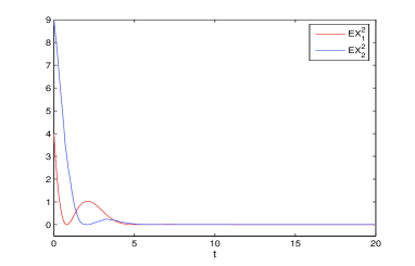
Figure 3: Second moment of the solution to Eq.(35) under DETM.

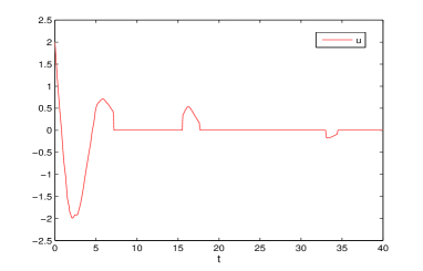
Figure 4: Response of switching control $u(t)$.

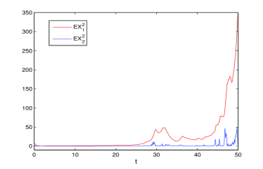
Figure 5: Second moment of the solution to Eq.(35) without control.

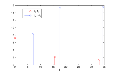
Figure 6: Inter-event times $s_{i}-t_{i}$ and $t_{i+1}-s_{i}$.

7 Conclusions and future research prospects

To obtain the stabilization and boundedness of stochastic nonlinear systems, we propose a switching control law based on a novel DETM. The advantage of DETM is that it can generate two stopping time series to realize the control updating and switching. Also, in DETM, the minimum inter-event time is guaranteed to be bounded by a positive constant to avoid the Zeno phenomenon. The switching control law based on DETM admits two different controls and extends the traditional aperiodic intermittent control. However, in this paper, the secondary control has little effect on stabilization because we choose a continuous primary control. In the future work, we will consider the primary control to be zero-order-hold. Then, the effectiveness of the secondary control will be highlighted.

References

- [1] C. Fei, W. Fei, X. Mao, D. Xia and L. Yan. Stabilization of highly nonlinear hybrid systems by feedback control based on discrete-time state observations. IEEE Trans. Automat. Control, 2020, 65: 2899-2912.
- [2] A. Cetinkaya and T. Hayakawa. A sampled-data approach to pyragas-type delayed feedback stabilization of periodic orbits. IEEE Trans. Automat. Control, 2019, 64: 3748-3755.
- [3] X. Mao. Stabilization of continuous-time hybrid stochastic differential equations by discrete-time feedback control. Automatica, 2013, 49: 3677-3681.
- [4] Y. Gao, X. Sun, C. Wen and W. Wang. Estimation of sampling period for stochastic nonlinear sampled-data systems with emulated controllers. IEEE Trans. Automat. Control, 2017, 62: 4713-4718.
- [5] X. Guo, D. Zhang, J. Wang, J. Park and L. Guo. Observer-based event-triggered composite anti-disturbance control for multi-agent systems under multiple disturbances and stochastic FDIAs. IEEE Trans. Autom. Sci. Eng., 2023, 20: 528-540.
- [6] X. Li, W. Liu, Q. Luo and X. Mao. Stabilisation in distribution of hybrid stochastic differential equations by feedback control based on discrete-time state observations. Automatica, 2022, 140, 110210.
- [7] X. Yang and Q. Zhu. Stabilization of stochastic retarded systems based on sampled-data feedback control. IEEE Trans. Syst., Man, Cybern., Syst., 2021, 51: 5895-5904.
- [8] S. Li, J. Guo and Z. Xiang. Global stabilization of a class of switched nonlinear systems under sampled-data control. IEEE Trans. Syst., Man, Cybern., Syst., 2019, 49: 1912-1919.
- [9] J. Sun, J. Yang, S. Li and Z. Zeng. Predictor-based periodic event-triggered control for dual-rate networked control systems with disturbances. IEEE Trans. Cybern., 2022, 52: 8179-8190.
- [10] C. Li, G. Feng and X. Liao. Stabilization of nonlinear systems via periodically intermittent control. IEEE Trans. Circuits Syst. II, Exp. Briefs, 2007, 54: 1019-1023.
- [11] Y. Li and C. Li. Complete synchronization of delayed chaotic neural networks by intermittent control with two switches in a control period. Neurocomputing, 2016, 173: 1341-1347.
- [12] X. Liu and T. Chen. Synchronization of complex networks via aperiodically intermittent pinning control. IEEE Trans. Automat. Control, 2015, 60: 3316-3321.
- [13] B. Liu, M. Yang, T. Liu and D. Hill. Stabilization to exponential input-to-state stability via aperiodic intermittent control. IEEE Trans. Automat. Control, 2021, 66: 2913-2919.
- [14] Y. Zhao and J. Fu. composite anti-bump switching control for switched systems. IEEE Trans. Syst., Man, Cybern., Syst., Early Access, 2021, 1-9.
- [15] B. Niu, D. Wang, H. Li, X. Xie, N. Alotaibi and F. Alsaadi. A novel neural-network-based adaptive control scheme for outputconstrained stochastic switched nonlinear systems. IEEE Trans. Syst., Man, Cybern., Syst., 2019, 49: 418-432.
- [16] X. Xiao, J. Park, L. Zhou and G. Lu. Event-triggered control of discrete-time switched linear systems with network transmission delays. Automatica, 2020, 111, 108585.
- [17] J. Wen, S. Nguang, P. Shi and L. Peng. Finite-time stabilization of Markovian jump delay systems-a switching control approach. Int. J. Robust Nonlinear Control, 2017, 27: 298-318.
- [18] Y. Chen and W. Zheng. Stability analysis and control for switched stochastic delayed systems. Int. J. Robust Nonlinear Control, 2016, 26: 303-328.
- [19] I. Haidar and P. Pepe. Lyapunov-Krasovskii charaterization of the input-to-state stability for switching retarded systems. SIAM J. Control Optim., 2021, 59: 2997-3016.
- [20] C. Viel, M. Kieffer, H. Piet-Lahanier and S. Bertrand. Distributed event-triggered formation control for multi-agent systems in presence of packet losses. Automatica, 2022, 141, 110215.
- [21] X. Li and P. Li. Input-to-state stability of nonlinear systems: event-triggered impulsive control. IEEE Trans. Automat. Control, 2022, 67: 1460-1465.
- [22] K. Zhang, B. Gharesifard and E. Braverman. Event-triggered control for nonlinear time-delay systems. IEEE Trans. Automat. Control, 2022, 67: 1031-1037.
- [23] X. Xu, A. Tahir and B. Açıkmeşe. Periodic event-triggered control for incrementally quadratic nonlinear systems. Int. J. Robust Nonlinear Control, 2021, 31: 5261-5280.
- [24] H. Zhao, W. Li, Z. Li and Y. Ren. Dynamic event-triggered control for Markovian jump linear systems with time-varying delay. Int. J. Robust Nonlinear Control, 2022, 32: 2359-2379.
- [25] S. Luo and F. Deng. On event-triggered control of nonlinear stochastic systems. IEEE Trans. Automat. Control, 2020, 65: 369-375.
- [26] Q. Zhu and T. Huang. control of stochastic networked control systems with time-varying delays: The event-triggered sampling case. Int. J. Robust Nonlinear Control, 2021, 31: 9767-9781.
- [27] W. Su, B. Niu, Y. Zhang, J. Zhang and Y. Li. Event-triggered adaptive decentralized control of stochastic nonlinear systems with strong interconnections and time-varying full-state constraints. Int. J. Robust Nonlinear Control, 2022, 32: 5200-5225.
- [28] D. Quevedo, V. Gupta, W. Ma and S. Yuksel. Stochastic stability of event-triggered anytime control. IEEE Trans. Automat. Control, 2014, 59: 3373-3379.
- [29] S. Luo. Stability and -gain analysis of linear periodic event-triggered systems with large delays. IEEE Trans. Circuits Syst. II, Exp. Briefs, Early Access, 2022, 1-5.
- [30] Y. Wang, W. Zheng and H. Zhang. Dynamic event-based control of nonlinear stochastic systems. IEEE Trans. Automat. Control, 2017, 62: 6544-6551.
- [31] Q. Zhu. Stabilization of stochastic nonlinear delay systems with exogenous disturbances and the event-triggered feedback control. IEEE Trans. Automat. Control, 2019, 64: 3764-3771.
- [32] F. Forni, S. Galeani, D. Nešić and L. Zaccarian. Event-triggered transmission for linear control over communication channels. Automatica, 2014, 50: 490-498.
- [33] A. Selivanov and E. Fridman. Event-triggered control: A switching approach. IEEE Trans. Automat. Control, 2016, 61: 3221-3226.