A Simple Method for
Predicting Covariance Matrices
of Financial Returns

Abstract

We consider the well-studied problem of predicting the time-varying covariance matrix of a vector of financial returns. Popular methods range from simple predictors like rolling window or exponentially weighted moving average (EWMA) to more sophisticated predictors such as generalized autoregressive conditional heteroscedastic (GARCH) type methods. Building on a specific covariance estimator suggested by Engle in 2002, we propose a relatively simple extension that requires little or no tuning or fitting, is interpretable, and produces results at least as good as MGARCH, a popular extension of GARCH that handles multiple assets. To evaluate predictors we introduce a novel approach, evaluating the regret of the log-likelihood over a time period such as a quarter. This metric allows us to see not only how well a covariance predictor does over all, but also how quickly it reacts to changes in market conditions. Our simple predictor outperforms MGARCH in terms of regret. We also test covariance predictors on downstream applications such as portfolio optimization methods that depend on the covariance matrix. For these applications our simple covariance predictor and MGARCH perform similarly.

Kasper Johansson
Stanford University
kasperjo@stanford.edu and Mehmet G. Ogut
Stanford University
giray98@stanford.edu and Markus Pelger
Stanford University
mpelger@stanford.edu and Thomas Schmelzer
Stanford University
Abu Dhabi Investment Authority
thomas.schmelzer@adia.ae and Stephen Boyd
Stanford University
boyd@stanford.edu copyrightowner=A. Heezemans and M. Casey, volume = xx, issue = xx, pubyear = 2023, isbn = xxx-x-xxxxx-xxx-x, eisbn = xxx-x-xxxxx-xxx-x, doi = 10.1561/XXXXXXXXX, firstpage = 1, lastpage = 87 cov_pred_finance.bib 1]Department of Electrical Engineering, Stanford University; kasperjo@stanford.edu 2]Department of Electrical Engineering, Stanford University; giray98@stanford.edu 3]Department of Management Science and Engineering, Stanford University; mpelger@stanford.edu 4]Department of Electrical Engineering, Stanford University, and Abu Dhabi Investment Authority; thomas.schmelzer@adia.ae 5]Department of Electrical Engineering, Stanford University; boyd@stanford.edu

Chapter 1 Introduction

1.1 Covariance prediction

We consider cross-sections, e.g., a vector time series of $n$ financial returns, denoted $r_{t}\in{\mbox{\bf R}}^{n}$, $t=1,2,\ldots$, where $(r_{t})_{i}$ is the return of asset $i$ from $t-1$ to $t$. We focus on the case where the mean $\mathop{\bf E{}}r_{t}$ is small enough that the second moment $\mathop{\bf E{}}r_{t}r_{t}^{T}\in{\mbox{\bf R}}^{n\times n}$ is a good approximation of the covariance matrix $\mathop{\bf cov{}}(r_{t})=\mathop{\bf E{}}r_{t}r_{t}^{T}-(\mathop{\bf E{}}r_{t})(\mathop{\bf E{}}r_{t})^{T}$, where $\mathop{\bf E{}}$ denotes expectation. This is the case for most daily, weekly, or monthly stock, bond, and futures returns, factor returns, and index returns. We start by focussing on the case where the number of assets $n$ is modest, say, on the order 10–100 or so; in chapter 8 we explain how to extend the method to much larger universes using ideas such as factor models.

We model the returns $r_{t}$ as independent random variables with zero mean and covariance $\Sigma_{t}\in{\mbox{\bf S}}_{++}^{n}$ (the set of symmetric positive definite matrices). We focus on the problem of predicting or estimating $\Sigma_{t}$, based on knowledge of $r_{1},\ldots,r_{t-1}$. The prediction is denoted as $\hat{\Sigma}_{t}\in{\mbox{\bf S}}_{++}^{n}$. The predicted volatilities of assets are given by

$$\hat{\sigma}_{t}=\mathop{\bf diag}(\hat{\Sigma}_{t})^{1/2}\in{\mbox{\bf R}}^{n},$$

where $\mathop{\bf diag}$ with a matrix argument is the vector of diagonal entries of the matrix, and the squareroot of a vector above is elementwise. We denote the predicted correlations as

$$\hat{R}_{t}=\mathop{\bf diag}(\hat{\sigma}_{t})^{-1}\hat{\Sigma}_{t}\mathop{\bf diag}(\hat{\sigma}_{t})^{-1},$$

where $\mathop{\bf diag}$ with a vector argument is the diagonal matrix with entries from the vector argument.

Covariance estimation comes up in several areas of finance, including Markowitz portfolio construction [markowitz_1952, grinold2000_portfolio], risk management [mcneil2015quantitative], and asset pricing [sharpe_1964]. Much attention has been devoted to this problem, and a Nobel Memorial Prize in Economic Sciences was awarded for work directly related to volatility estimation [engle_1982].

While it is well known that the tails of financial returns are poorly modeled by a Gaussian distribution, our focus here is on the bulk of the distribution, where the Gaussian assumption is reasonable. For future use, we note that the log-likelihood of an observed return $r_{t}$, under the Gaussian distribution $r_{t}\sim\mathcal{N}(0,\hat{\Sigma}_{t})$, is

$$l_{t}(\hat{\Sigma}_{t})=\frac{1}{2}\left(-n\log(2\pi)-\log\det\hat{\Sigma}_{t}-r_{t}^{T}\hat{\Sigma}_{t}^{-1}r_{t}\right).$$ (1.1)

The Gaussian log-likelihood is closely related to a popular metric for evaluating covariance predictors in econometrics, called the (Gaussian) quasi-likelihood (QLIKE) [patton2011volatility, patton2009evaluating, laurent2013loss]. QLIKE is the negative log-likelihood, under the Gaussian assumption, up to an additive constant and a positive scale factor. Roughly speaking, we seek covariance predictors that achieve large values of log-likelihood, or small values of QLIKE, on realized returns. We will describe evaluation of covariance predictors in detail in chapter 4.

1.2 Contributions

This monograph makes three contributions. First, we propose a new method for predicting the time-varying covariance matrix of a vector of financial returns, building on a specific covariance estimator suggested by Engle in 2002. Our method is a relatively simple extension that requires very little tuning and is readily interpretable. It relies on solving a small convex optimization problem, which can be carried out very quickly and reliably [boyd2004convex]. Our method performs as well as much more complex methods, as measured by several metrics.

Our second contribution is to propose a new method for evaluating a covariance predictor, by considering the regret of the log-likelihood over some time period such as a quarter. This approach allows us to evaluate how quickly a covariance estimator reacts to changes in market conditions.

Our third contribution is an extensive empirical study of covariance predictors. We compare our new method to other popular predictors, including rolling window, exponentially weighted moving average (EWMA), and generalized autoregressive conditional heteroscedastic (GARCH) type methods. We find that our method performs slightly better than other predictors. However, even the simplest predictors perform well for practical problems like portfolio optimization.

Everything needed to reproduce our results, together with an open source implementation of our proposed covariance predictor, is available online at

https://github.com/cvxgrp/cov_pred_finance.

1.3 Outline

In chapter 2 we describe some common predictors, including the one that our method builds on. We introduce our proposed covariance predictor in chapter 3. In chapter 4 we discuss methods for validating covariance predictors that measure both overall performance and reactivity to market changes. We describe the data we use in our first empirical studies in chapter 5, and give the results in chapter 6.

In the next chapters we discuss some extensions of and variations on our method, including realized covariance prediction (chapter 7), handling large universes via factor models (chapter 8), obtaining smooth covariance estimates (chapter 9), and using our covariance model to generate simulated returns (chapter 10).

Chapter 2 Some common covariance predictors

In this chapter we review some common covariance predictors, ranging from simple to complex, with the goal of giving context and fixing our notation. To simplify some formulas, we take $r_{\tau}=0$ for $\tau\leq 0$.

2.1 Rolling window

The rolling window predictor with window length or memory $M$ is the average of the last $M\geq n$ outer products,

$$\hat{\Sigma}_{t}=\alpha_{t}\sum_{\tau=t-M}^{t-1}r_{\tau}r_{\tau}^{T},\quad t=2,3,\ldots,$$

where $\alpha_{t}=1/\min\{t-1,M\}$ is the normalization constant. The rolling window predictor can be evaluated via the recursion

$$\hat{\Sigma}_{t+1}=\frac{\alpha_{t+1}}{\alpha_{t}}\hat{\Sigma}_{t}+\alpha_{t+1}(r_{t}r_{t}^{T}-r_{t-M}r_{t-M}^{T}),\quad t=1,2,\ldots,$$

with initialization $\hat{\Sigma}_{1}=0$.

For $t<n$, the rolling window covariance estimate is not full rank. To handle this, as well as to improve the quality of the prediction, we can add regularization or shrinkage, for example by adding a positive multiple of $\mathop{\bf diag}(\hat{\Sigma}_{t})$ to our estimate [ledoit110_honey_cov, ledoit2003improved], or approximating the predicted covariance matrix by a diagonal plus low rank matrix, as described in chapter 8.

2.2 EWMA

The exponentially weighted moving average (EWMA) estimator, with forgetting factor $\beta\in(0,1)$, is

$$\hat{\Sigma}_{t}=\alpha_{t}\sum_{\tau=1}^{t-1}\beta^{t-1-\tau}r_{\tau}r_{\tau}^{T},\quad t=2,3,\ldots,$$ (2.1)

where

$$\alpha_{t}=\left(\sum_{\tau=1}^{t-1}\beta^{t-1-\tau}\right)^{-1}=\frac{1-\beta}{1-\beta^{t-1}}$$

is the normalization constant. The forgetting factor $\beta$ is usually expressed in terms of the half-life $H=-\log 2/\log\beta$, for which $\beta^{H}=1/2$. The half-life $H$ is the number of periods when the exponential weight has decreased by a factor of two. For example, for a half-life of one year, the current observed return has twice the impact on our covariance prediction as the return observed one year ago. The EWMA predictor is widely used in practice; for example RiskMetrics suggests the forgetting factor $\beta=0.94$, which corresponds to a half-life of around 11 days [menchero2011barra, longerstaey1996riskmetrics].

The EWMA covariance predictor can be computed recursively as

$$\hat{\Sigma}_{t+1}=\frac{\beta-\beta^{t}}{1-\beta^{t}}\hat{\Sigma}_{t}+\frac{1-\beta}{1-\beta^{t}}r_{t}r_{t}^{T},\quad t=1,2,\ldots,$$

with initialization $\hat{\Sigma}_{1}=0$. Like the rolling window predictor, the EWMA predictor is singular for $t<n$, which can be handled using the same regularization methods described above.

2.3 GARCH and MGARCH

GARCH.

The generalized autoregressive conditional heteroscedastic (GARCH) predictor decomposes the return of a single asset as

$$r_{t}=\mu+\epsilon_{t},$$

where $\mu$ is the mean return and $\epsilon_{t}$ is the innovation, and models the innovation as

$$\epsilon_{t}=\sigma_{t}z_{t},\qquad\sigma_{t}^{2}=\omega+\sum_{\tau=1}^{q}a_{\tau}\epsilon_{t-\tau}^{2}+\sum_{\tau=1}^{p}b_{\tau}\sigma_{t-\tau}^{2},$$

where $\sigma_{t}$ is the asset volatility, $z_{t}$ are independent $\mathcal{N}(0,1)$, and $q$ and $p$ (often both set to one in practice) determine the GARCH order [bollerslev_1986]. (Recall that we assume zero mean.) The model parameters are $\omega$, $a_{1},\ldots,a_{q}$, and $b_{1},\ldots,b_{p}$. Estimating the model parameters requires solving a nonconvex optimization problem [cov_barrat_2022].

With $p=0$ we recover the autoregressive conditional heteroscedastic (ARCH) predictor, introduced in the seminal paper by engle_1982. This paper set the foundation for a wide variety of popular volatility and correlation predictors and earned him the 2003 Nobel Memorial Prize in Economic Sciences.

MGARCH.

There are several ways of extending the GARCH predictor to a multivariate or vector setting. The most popular is the dynamic conditional correlation (DCC) predictor [DCC], which is a two-step approach described below.

Many other MGARCH predictors have been proposed. The most straightforward generalization from the univariate to multivariate predictors is the VEC predictor, where the covariance matrix is vectorized and each element is modeled as a GARCH process with dependencies on all other elements [bollerslev_engle_1988]. However, this extension requires estimating $n(n+1)(n(n+1)+1)/2\approx n^{4}/2$ parameters, which can be impractical even for modest values of $n$.

Following the VEC extension of GARCH, multivariate GARCH (MGARCH) predictors have been proposed in two lines of development [silvennoinen2009multivariate]. The first line involves models that impose restrictions on the parameters of the VEC predictor, including DVEC [bollerslev_1986], BEKK [engle_kroner_1995], FF-MGARCH [FF_MGARCH], O-GARCH [OGARCH], and GO-GARCH [GOGARCH], to name some. However, these predictors have been shown to be hard to fit and can yield inconsistent estimates [brooks_2003]. (These inconsistencies may not have much practical impact.) For detailed reviews of MGARCH predictors we refer the reader to [silvennoinen2009multivariate, garch_survey]

2.4 DCC GARCH

The second line of extensions of GARCH to vector time series models conditional covariances through separate estimates of conditional variances and correlations [DCC, engle2001theoretical]. In [CCC] Bollerslev introduced the constant conditional correlation predictor (CCC) where the individual asset volatilities are modeled as separate GARCH processes, while the correlation matrix is assumed constant and equal to the unconditional correlation matrix. This predictor was later extended to the dynamic conditional correlation (DCC) predictor where the correlation matrix is allowed to change over time [DCC]. The DCC model has the form

$$\Sigma_{t}=D_{t}R_{t}D_{t},$$

where $D_{t}$ is the diagonal matrix of standard deviations, i.e., $(D_{t})_{ii}=(\Sigma_{t})_{ii}^{1/2}$, and $R_{t}$ is the correlation matrix associated with $\Sigma_{t}$.

DCC GARCH models the diagonal elements of $D_{t}$ as separate univariate GARCH processes as described above. The correlation matrix $R_{t}$ is then modeled as a constrained multivariate GARCH (MGARCH) process, e.g., as

$$R_{t} = \mathop{\bf diag}(\mathop{\bf diag}(Q_{t}))^{-1/2}Q_{t}\mathop{\bf diag}(\mathop{\bf diag}(Q_{t}))^{-1/2},$$

$$Q_{t} = \bar{Q}(1-a-b)+a\tilde{r}_{t}\tilde{r}_{t}^{T}+bQ_{t-1},$$

where $\bar{Q}$ is the unconditional correlation matrix, $a$ and $b$ are the MGARCH parameters, and $\tilde{r}_{t}$ are the volatility adjusted returns defined as

$$\tilde{r}_{t}=D_{t}^{-1}r_{t}.$$

The parameters can be estimated in two steps via (quasi) maximum likelihood, but requires solving non-convex optimization problems [DCC]. This predictor has become a popular choice amongst MGARCH predictors due to its interpretability. Variants of the DCC predictor are widely used in finance, where it is also often used in combination with EWMA estimates. Conditional correlation predictors are easier to estimate than other multivariate GARCH predictors, and their parameters are more interpretable.

Iterated covariance estimation.

DCC, which separately estimates the volatilities and correlations, is closely related to the idea of iterated covariance predictors [cov_barrat_2022]. Iterated covariance predictors estimate the covariance matrix in multiple iterations. In a two-step iteration we first form a first covariance estimate $\hat{\Sigma}_{t}^{(1)}$ of the returns $r_{t}$, at each time $t$, and form the whitened returns

$$\tilde{r}_{t}=\left(\hat{\Sigma}_{t}^{(1)}\right)^{-1/2}r_{t}.$$

In the second iteration we form the covariance estimate $\hat{\Sigma}_{t}^{(2)}$ of the whitened returns $\tilde{r}_{t}$. The final covariance estimate (of the returns $r_{t}$) is then formed as

$$\hat{\Sigma}_{t}=\left(\hat{\Sigma}_{t}^{(1)}\right)^{1/2}\hat{\Sigma}_{t}^{(2)}\left(\hat{\Sigma}_{t}^{(1)}\right)^{1/2}.$$

This procedure can be iterated further, and has been shown empirically to improve the quality of the covariance estimate; see [cov_barrat_2022] for details. In DCC, $\hat{\Sigma}^{(1)}$ is diagonal and models the volatilities; $\hat{\Sigma}^{(2)}$ is a correlation matrix.

2.5 Iterated EWMA

Iterated EWMA (IEWMA) was proposed by [DCC] and is analogous to DCC GARCH but with EWMA estimates of the volatilities and correlations instead of GARCH. Engle proposed IEWMA as an efficient alternative to the DCC GARCH predictor, although he did not refer to it as IEWMA; we use this term to emphasize its connection to iterated whitening, as proposed in [cov_barrat_2022]. Specifically, IEWMA can be viewed as an iterated whitener, where we first use a diagonal whitener (which estimates the volatilities) and then a full matrix whitener (which estimates the correlations). This is analogous to the two-step iterated covariance predictor where $\hat{\Sigma}_{t}^{(1)}$ is the diagonal matrix of squared volatility estimates and $\hat{\Sigma}_{t}^{(2)}$ estimates the correlation matrix of the volatility adjusted returns.

First we form an estimate of the volatilities $\hat{\sigma}_{t}=\mathop{\bf diag}(\hat{\Sigma}_{t})^{1/2}$ using EWMA predictors for each asset. We denote the half-life of these volatility estimates as $H^{\text{vol}}$. We then form the marginally standardized returns as

$$\tilde{r}_{t}=\hat{D}_{t}^{-1}r_{t},$$ (2.2)

where $\hat{D}_{t}=\mathop{\bf diag}(\hat{\sigma}_{t})$. These vectors should have entries with standard deviation near one. It is common practice to winsorize the standardized returns; a good rule of thumb is to clip $\tilde{r}_{t}$ at $\pm 4.2$, which corresponds to clipping $r_{t}$ at $\pm 4.2\hat{\sigma}_{t}$.

Then we form a EWMA estimate of the covariance of $\tilde{r}_{t}$, which we denote as $\tilde{R}_{t}$, using half-life $H^{\text{cor}}$ for this EWMA estimate. (We use the superscript ‘cor’ since the diagonal entries of $\tilde{R}_{t}$ should be near one, so $\tilde{R}_{t}$ is close to a correlation matrix.) From $\tilde{R}_{t}$ we form its associated correlation matrix $\hat{R}_{t}$, i.e., we scale $\tilde{R}_{t}$ on the left and right by a diagonal matrix with entries $(\tilde{R}_{t})_{ii}^{-1/2}$. Since the diagonal entries of $\tilde{R}_{t}$ should be near one, $\tilde{R}_{t}$ and $\hat{R}_{t}$ are not too different.

Our IEWMA covariance predictor is

$$\hat{\Sigma}_{t}=\hat{D}_{t}\hat{R}_{t}\hat{D}_{t},\quad t=2,3,\ldots.$$

This is the covariance predictor proposed in [DCC]; replacing $\hat{R}_{t}$ with $\tilde{R}_{t}$ we obtain the iterated whitener proposed by Barratt and Boyd in [cov_barrat_2022]. As mentioned above, they are typically quite close.

It is common to choose the volatility half-life $H^{\text{vol}}$ to be smaller than the correlation half-life $H^{\text{cor}}$. The intuition here is that we can average over fewer past samples when we predict the $n$ volatilities $\hat{\sigma}_{t}$, but need more past samples to reliably estimate the $n(n-1)/2$ off-diagonal entries of $\hat{R}_{t}$. Empirical studies on real return data confirm that choosing a faster volatility half-life than correlation half-life yields better estimates.

Chapter 3 Combined multiple iterated EWMAs

In this chapter we introduce a novel covariance predictor, which we call combined multiple iterated EWMAs, for which we use the acronym CM-IEWMA. The CM-IEWMA predictor is constructed from a modest number of IEWMA predictors, with different pairs of half-lives, which are combined using dynamically varying weights that are based on recent performance.

The CM-IEWMA predictor is motivated by the idea that different pairs of half-lives may work better for different market conditions. For example, short half-lives perform better in volatile markets, while long half-lives perform better for calm markets where conditions are changing slowly.

3.1 Dynamically weighted prediction combiner

We first describe the idea in a general setting. We start with $K$ different covariance predictors, denoted $\hat{\Sigma}^{(k)}_{t}$, $k=1,\ldots,K$. These could be any of the predictors described above, or predictors of the same type with different parameter values, e.g., half-lives (for EWMA) or pairs of half-lives (for IEWMA). In some contexts these different predictors are referred to as a set of $K$ experts [hastie2009elements, jordan1994hierarchical].

We denote the Cholesky factorizations of the associated precision matrices $(\hat{\Sigma}_{t}^{(k)})^{-1}$ as $\hat{L}_{t}^{(k)}$, i.e.,

$$\left(\hat{\Sigma}_{t}^{(k)}\right)^{-1}=\hat{L}_{t}^{(k)}(\hat{L}_{t}^{(k)})^{T},\quad k=1,\ldots,K,$$

where $\hat{L}_{t}^{(k)}$ are lower triangular with positive diagonal entries. We will combine these Cholesky factors with nonnegative weights $\pi_{1},\ldots,\pi_{K}$ that sum to one, to obtain

$$\hat{L}_{t}=\sum_{k=1}^{K}\pi_{k}\hat{L}_{t}^{(k)}.$$ (3.1)

From this we recover the weighted combined predictor

$$\hat{\Sigma}_{t}=\left(\hat{L}_{t}\hat{L}_{t}^{T}\right)^{-1}.$$ (3.2)

We will see below why we combine the Cholesky factors of the precision matrices, and not the covariance or precision matrices themselves.

3.2 Choosing the weights via convex optimization

The log-likelihood (1.1) can be expressed in terms of the Cholesky factor of the precision matrix $\hat{L}_{t}$ as

$$l_{t}(\hat{\Sigma}_{t})=-(n/2)\log(2\pi)+\sum_{i=1}^{n}\log\hat{L}_{t,ii}-(1/2)\|\hat{L}^{T}_{t}r_{t}\|^{2}_{2},$$

where $\|\cdot\|_{2}$ denotes the Euclidean norm. This is a concave function of the weights $\pi\in{\mbox{\bf R}}_{+}^{K}$ [boyd2004convex].

We choose the weights at time $t$ as the solution of the convex optimization problem

$$\begin{array}[]{ll}\mbox{maximize}&\sum_{j=1}^{N}\bigg{(}\sum_{i=1}^{n}\log\hat{L}_{t-j,ii}-(1/2)\|\hat{L}^{T}_{t-j}r_{t-j}\|^{2}_{2}\bigg{)}\\ \mbox{subject to}&\hat{L}_{\tau}=\sum_{j=1}^{K}\pi_{j}\hat{L}_{\tau}^{(j)},\quad\tau=t-1,\dots,t-N\\ &\pi\geq 0,\quad\mathbf{1}^{T}\pi=1,\end{array}$$ (3.3)

with variables $\pi_{1},\ldots,\pi_{K}$, where $N$ is the look-back, $\mathbf{1}$ denotes the vector with entries one, and $\geq$ between vectors means entrywise. In words: we choose the (mixture) weights in each period so as to maximize the average log-likelihood of the combined prediction over the trailing $N$ periods. The problem (3.3) is convex, and can be solved very quickly and reliably by many methods [boyd2004convex]. The covariance predictor is then recovered using (3.1) and (3.2).

The look-back $N$ is a parameter that can be adjusted to give good performance. Numerical experiments suggest that the predictor is not very sensitive to the choice of $N$, and that a choice $N=10$ seems to work well for asset universes up to a few hundred assets.

We mention several extensions of the weight problem (3.3). First, we can add one prediction which is diagonal, using any estimates of the volatilities (including constant). This gives us shrinkage, automatically chosen. We can also add a constraint or objective term that encourages the weights to vary smoothly over time, as discussed more in chapter 9.

The CM-IEWMA predictor is a special case of the dynamically weighted prediction combiner described above, where the $K$ predictions are each IEWMA, with different pairs of half-lives $H^{\text{vol}}$ and $H^{\text{cor}}$.

Chapter 4 Evaluating covariance predictors

There are several ways of evaluating a covariance predictor, often divided into two categories, direct and indirect [patton2009evaluating], [ANDERSEN2006777, §7]. Direct methods use a proxy for the true covariance matrix to evaluate the predictor, while indirect methods use the covariance predictor on tasks of interest, such as portfolio construction or portfolio tracking.

Popular direct methods are the Mincer-Zarnowitz (MZ) regression and its variants, based on statistical tests of the regression coefficients of a predicted variable on an observed variable (or in the case of variance and covariance, a proxy for the observed variable) [mincer1969evaluation, theil1961economic]. Direct methods also include the comparison between different predictors in terms of some loss function. Common loss functions are the mean squared error (MSE) and quasi-likelihood (QLIKE) [patton2011volatility, patton2009evaluating]. To select good models, the model confidence set (MCS) is usually used [hansen2011model], or the Ledoit–Wolf test [ledoit2008robust] to compare Sharpe ratios.

Indirect methods use applications to rank covariance predictors, and include the minimum variance and mean-variance portfolios, as well as portfolio tracking tasks.

The difference in performance between various predictors can also be evaluated using statistical tests. For a more detailed discussion of both direct and indirect methods, we refer the reader to [patton2009evaluating].

In this chapter we discuss several evaluation metrics for covariance predictors. The first three metrics are direct, and include the mean squared error and two metrics based on a statistical measure, the log-likelihood under a Gaussian distribution. The remaining metrics judge a covariance predictor by the performance of a portfolio using a method that depends on a covariance matrix. We are mainly interested in illustrating how simple methods can perform just as well as or better than more complex ones, rather than finding optimal predictors in a statistical sense. Therefore we look at the absolute performance of covariance predictors on these metrics.

4.1 Mean squared error

The mean squared error (MSE) is a common metric for evaluating a covariance predictor $\hat{\Sigma}_{t}$, defined as

$$\frac{1}{T}\sum_{t=1}^{T}\|r_{t}r_{t}^{T}-\hat{\Sigma}_{t}\|_{F}^{2},$$

i.e., the average squared Frobenius norm of the difference between the realized (rank one) covariance matrix $r_{t}r_{t}^{T}$ and the covariance predictor $\hat{\Sigma}_{t}$. Lower values of MSE are better. One variation on the MSE error assumes that $\hat{\Sigma}_{t}$ is constant over some number of time periods and replaces the rank one realized covariance $r_{t}r_{t}^{T}$ with an average of the rank one terms over the periods, i.e., the realized empirical covariance.

4.2 Log-likelihood

A natural way of judging a covariance predictor is via its average log-likelihood on realized returns,

$$\frac{1}{2T}\sum_{t=1}^{T}\Big{(}-n\log(2\pi)-\log\det\hat{\Sigma}_{t}-r_{t}^{T}\hat{\Sigma}_{t}^{-1}r_{t}\Big{)},$$

with larger values being better. This metric can be used to compare different predictors.

To understand the performance of a covariance predictor over time and changing market conditions, we can examine the average log-likelihood over periods such as quarters, and look at the distribution of quarterly average log-likelihood values. We are particularly interested in poor, i.e., low values.

4.3 Log-likelihood regret

Recall that the best constant predictor, in terms of the log-likelihood, is the empirical sample covariance

$$\Sigma^{\text{emp}}=\frac{1}{T}\sum_{t=1}^{T}r_{t}r_{t}^{T},$$

with value

$$\frac{1}{2}\big{(}-n(\log(2\pi)+1)-\log\det\Sigma^{\text{emp}}\big{)}.$$

For any other constant $\Sigma\in{\mbox{\bf S}}_{++}^{n}$, the log-likelihood is lower than the log-likelihood of $\Sigma^{\text{emp}}$. We define the average log-likelihood regret as the average log-likelihood of the (constant) empirical covariance, minus the average log-likelihood of the covariance predictor. The regret is a measure of how much the covariance predictor $\hat{\Sigma}_{t}$, $t=1,\ldots,T$, underperforms the best possible constant covariance predictor (i.e., the sample covariance matrix). The term regret comes from the field of online optimization; see, e.g., [zinkevich2003_regret, Mokhtari2016_regret, hazan2007_regret, hazan2016introduction].

We want our covariance predictor to have small regret. The regret is typically positive, but it can be negative, i.e., our time-varying covariance can have higher log-likelihood than the best constant one. The regret is not any more useful than the log-likelihood when comparing predictors over one time interval, since it simply adds a constant and switches the sign. But it is interesting when we compute the regret over multiple periods, like months or quarters. The regret over multiple quarters removes the effect of the log-likelihood of the empirical covariance varying due to changing market conditions, and allows us to assess how well the covariance predictor adapts.

4.4 Portfolio performance

We can also judge the performance of a covariance predictor by the investment performance of portfolio construction methods that depend on the estimated covariance matrix. As with log-likelihood or log-likelihood regret, we can examine the portfolio performance in periods such as quarters, to see how evenly the performance is spread over time.

One obvious metric of interest is how close the ex-ante and realized portfolio volatilities are. The metrics described above, MSE, log-likelihood, and log-likelihood regret, are agnostic to the portfolio; with specific real portfolios we can see how well our covariance predictors predict portfolio volatility.

We will assess a covariance predictor using five simple portfolio construction methods. The first is an equally weighted (or $1/n$) portfolio, which does not by itself depend on the covariance, but does when we adjust it with cash to achieve a given ex-ante risk. The second, third, and fourth portfolios depend only on the covariance matrix. They are minimum variance, risk parity, and maximum diversification portfolios. For an in depth discussion of these portfolios, see [braga2015risk]. The last portfolio we consider is a mean-variance portfolio, using a very simple mean estimator.

For each portfolio we look at four metrics: realized return, volatility, Sharpe ratio, and maximum drawdown. The returns, volatilities, and Sharpe ratios are reported in annualized values. The Sharpe ratio is defined as the ratio of the excess return (over the risk-free rate), divided by the volatility of the excess return,

$$\frac{\frac{1}{T}\sum_{\tau=1}^{T}(r^{p}_{t}-r^{\text{rf}}_{t})}{\Big{(}\frac{1}{T}\sum_{\tau=1}^{T}\big{(}r^{p}_{t}-\frac{1}{T}\sum_{\tau=1}^{T}r^{p}_{t}\big{)}^{2}\Big{)}^{1/2}},$$

where $r^{p}_{t}$ and $r^{\text{rf}}_{t}$ are the portfolio and risk-free returns at time $t$. The maximum drawdown is defined as

$$\max_{1\leq t_{1}<t_{2}\leq T}\frac{V^{p}_{t_{1}}}{V^{p}_{t_{2}}}-1,$$

where

$$V^{p}_{t}=V_{0}(1+r^{p}_{1})(1+r^{p}_{2})\cdots(1+r^{p}_{t})$$

is the portfolio value at time $t$ (with returns re-invested), starting with value $V_{0}>0$.

In addition to portfolio performance, we can also examine how well the covariance prediction predicts the portfolio volatility. We compare the realized or ex-post portfolio volatility

$$\left(\frac{1}{T}\sum_{t=1}^{T}(r_{t}^{T}w_{t})^{2}\right)^{1/2},$$

to the predicted or ex-ante portfolio volatility

$$\left(\frac{1}{T}\sum_{t=1}^{T}w_{t}^{T}\hat{\Sigma}_{t}w_{t}\right)^{1/2},$$

where $w_{t}\in{\mbox{\bf R}}^{n}$ are the portfolio weights. This directly measures the ability of the estimated covariance matrix to predict portfolio risk.

Equal weight portfolio.

We take the equal weight or $1/n$ portfolio with $w=(1/n)\mathbf{1}$. This portfolio does not depend on the covariance $\hat{\Sigma}_{t}$, but when we mix it with cash, as described below, it will.

Minimum variance portfolio.

The (constrained) minimum variance portfolio is the solution of the convex optimization problem

$$\begin{array}[]{ll}\mbox{minimize}&\quad w^{T}\hat{\Sigma}_{t}w\\ \mbox{subject to}&\quad w^{T}\mathbf{1}=1,\quad\|w\|_{1}\leq L_{\max},\quad w_{\min}\leq w\leq w_{\max}\end{array}$$

with variable $w\in{\mbox{\bf R}}^{n}$, where $L_{\max}\geq 1$ is a leverage limit, and $w_{\min}$ and $w_{\max}$ are lower and upper bounds on the weights, respectively.

Risk-parity portfolio.

The portfolio return volatility $\sigma(w)=(w^{T}\hat{\Sigma}_{t}w)^{1/2}$ can be broken down into a sum of volatilities (risks) associated with each asset as

$$\frac{\partial\log\sigma(w)}{\partial w_{i}}=\frac{\partial\sigma(w)}{\sigma(w)}\frac{w_{i}}{\partial w_{i}}=\frac{w_{i}(\hat{\Sigma}_{t}w)_{i}}{w^{T}\hat{\Sigma}_{t}w},\quad i=1,\dots,n.$$

The risk parity portfolio is the one for which these volatility attributions are equal [Qian119]. This portfolio can be found by solving the convex optimization problem [cvx_book_additional],

$$\mbox{minimize}\quad(1/2)x^{T}\hat{\Sigma}_{t}x-\sum_{i=1}^{n}(1/n)\log x_{i},$$

with variable $x$, and then taking $w=x^{\star}/(\mathbf{1}^{T}x^{\star})$.

Maximum diversification portfolio.

The diversification ratio of a long-only portfolio (i.e., one with $w\geq 0$) is defined as

$$D(w)=\frac{\hat{\sigma}_{t}^{T}w}{(w^{T}\hat{\Sigma}_{t}w)^{1/2}}.$$

The diversification ratio tells us how much higher the portfolio volatility would be if all assets were perfectly correlated. The maximum diversification portfolio is the portfolio $w$ that maximizes $D(w)$, possibly subject to constraints [choueifaty2008toward]. Like the risk-parity portfolio, the maximum diversification portfolio can be found via convex optimization. We let $x^{\star}$ denote the solution of the convex optimization problem [cvx_book_additional]

$$\begin{array}[]{ll}\mbox{minimize}&x^{T}\hat{\Sigma}_{t}x\\ \mbox{subject to}&\hat{\sigma}_{t}^{T}x=1,\quad x\geq 0,\end{array}$$

with variable $x$. The maximum diversification portfolio is $w=x^{\star}/\mathbf{1}^{T}x^{\star}$.

Volatility control with cash.

We mix each of the four portfolios described above with cash to achieve a target value of ex-ante volatility $\sigma^{\mathrm{tar}}$. To do this we start with the portfolio weight vector $w_{t}$, and compute its ex-ante volatility $\sigma_{t}=(w_{t}^{T}\hat{\Sigma}_{t}w_{t})^{1/2}$. Then we add a cash component so that the overall ex-ante volatility equals our target, i.e., we use the $(n+1)$ weights (with the last component denoting cash)

$$\left[\begin{array}[]{c}\theta w_{t}\\ (1-\theta)\end{array}\right],\qquad\theta=\frac{\sigma^{\text{tar}}}{\sigma_{t}}.$$

This portfolio will have ex-ante volatility $\sigma^{\mathrm{tar}}$. Note that the cash weight can be either positive (when it dilutes the portfolio volatility) or negative (when it leverages the portfolio volatility to the desired level). The target volatility $\sigma^{\text{tar}}$ should be chosen so as to avoid portfolios that are either too diluted or too leveraged.

Mean variance portfolio.

The last portfolio we consider is a basic mean-variance portfolio, defined as the solution of the convex optimization problem

$$\begin{array}[]{ll}\mbox{maximize}&\quad\hat{r}_{t}^{T}w\\ \mbox{subject to}&\quad\|\hat{\Sigma}_{t}^{1/2}w\|_{2}\leq\sigma^{\text{tar}}\\ &\quad\mathbf{1}^{T}w+c=1,\quad\|w\|_{1}\leq L_{\max},\\ &\quad w_{\min}\leq w\leq w_{\max},\quad c_{\min}\leq c\leq c_{\max}\end{array}$$

with variable $w$, where $\hat{r}_{t}$ is the predicted mean return vector at time $t$. The vector $w$ gives the weights of the non-cash assets and $c$ denotes the cash weight. The non-cash and cash weights are limited by $w_{\min},w_{\max}$ and $c_{\min},c_{\max}$, respectively. This portfolio does not need cash dilution, since it includes cash in its construction. (If $\sigma^{\text{tar}}$ is chosen appropriately, it will have ex-ante risk $\sigma^{\text{tar}}$.) The mean-variance portfolio depends not only on a covariance estimate, but also a return estimate. For this we use one of the simplest possible return estimates, a EWMA of the realized returns.

Chapter 5 Data sets and experimental setup

We illustrate our method on three different data sets: a set of $49$ industry portfolios, a set of $25$ stocks, and a set of $5$ factor returns, each augmented with cash (with the historical risk-free interest rate). For each data set we show results for six covariance predictors. Everything needed to reproduce the results is available online at

https://github.com/cvxgrp/cov_pred_finance.

5.1 Data sets

Industry portfolios.

The first data set consists of the daily returns of a universe of $n=49$ daily traded industry portfolios, shown in table 5.1, along with cash. The data set spans July 1st 1969 to December 30th, 2022, for a total of 13496 (trading) days. The data was obtained from the Kenneth French Data Library [french_data_lib].

Table 5.1: Industry portfolios.

Agriculture Food products Candy & soda Beer & liquor Tobacco products Recreation Entertainment Printing and publishing Consumer goods Apparel Healthcare Medical equipment Pharmaceutical products Chemicals Rubber and plastic products Textiles Construction materials Construction Steel works etc. Fabricated products Machinery Electrical equipment Automobiles and trucks Aircraft Shipbuilding, railroad equipment Defense Precious metals Non-metallic and industrial metal mining Coal Petroleum and natural gas Utilities Communication Personal services Business services Computers Computer software Electronic equipment Measuring and control equipment Business supplies Shipping containers Transportation Wholesale Retail Restaurants, hotels, motels Banking Insurance Real estate Trading Other

Stocks.

The second data set consists of the daily returns of $n=25$ stocks and cash. The stocks were chosen to be the 25 largest stocks in the S&P 500 at the beginning of 2010, listed in table 5.2. This data set spans January 4th 2010 to December 30th, 2022, for a total of 3272 (trading) days. The stock data was attained through the Wharton Research Data Services (WRDS) portal [WRDS].

Table 5.2: List of companies and their tickers.

Ticker	Company Name
XOM	Exxon Mobil
WMT	Walmart
AAPL	Apple Inc.
PG	Procter & Gamble
JNJ	Johnson & Johnson
CHL	China Mobile
IBM	IBM
SBC	AT&T
GE	General Electric
CHV	Chevron
PFE	Pfizer
NOB	Noble
NCB	NCR
KO	Coca-Cola
ORCL	Oracle Corporation
HWP	Hewlett-Packard
INTC	Intel Corporation
MRK	Merck & Co.
PEP	PepsiCo
BEL	Becton, Dickinson and Company
ABT	Abbott Laboratories
SLB	Schlumberger
P	Pandora Media
PA	Pan American Silver
MCD	McDonald’s

Factor returns.

The third data set consists of daily returns of the five Fama-French factors taken from the Kenneth French Data Library [french_data_lib], shown in table 5.3. The data set spans July 1st 1963 to December 30th, 2022, for a total of 14979 (trading) days.

Table 5.3: The five Fama-French factors.

Factor Description MKT-Rf market excess return over risk-free rate SMB small stocks minus big stocks HML high book-to-market stocks minus low book-to-market stocks RMW stocks with high operating profitability minus stocks with low operating profitability CMA stocks with conservative investment policies minus stocks with aggressive investment policies

Cumulative returns.

In figure 5.1 we show the cumulative returns of the five factors, and the cumulative returns of five assets chosen from each of the industry and stock data sets.

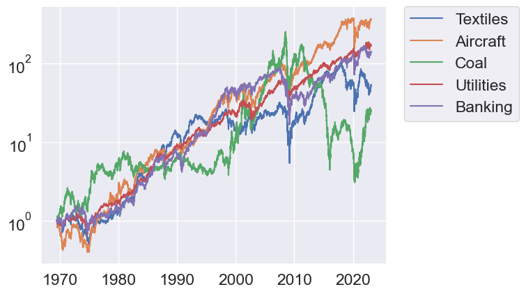
(a) Industry data set.

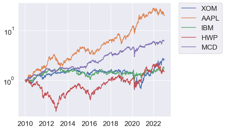
(b) Stock data set.

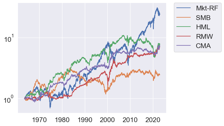
(c) Factor data set.

Figure 5.1: Cumulative returns of five assets from each data set.

5.2 Six covariance predictors

For each data set we evaluate six covariance predictors, described below.

• Rolling window estimates with 500-, 250-, and, 125-day windows for the industry, stock, and factor data sets, respectively, denoted RW in plots and tables.

• EWMA predictors with 250-, 125-, and, 63-day half-lives, for the industry, stock, and factor data sets, respectively, denoted EWMA.

• IEWMA predictors with half-lives (in days) $H^{\text{vol}}/H^{\text{cor}}$ of 125/250, 63/125, and 21/63 for the three data sets, respectively, denoted IEWMA.

• DCC GARCH predictor, denoted MGARCH, with parameters re-estimated annually using the rmgarch package in R [ghalanos2019rmgarch].

• CM-IEWMA predictor with $K=5$ IEWMA predictors and a lookback of $N=10$ days, with half-lives shown in table 5.4. For each of the fastest IEWMA predictors we regularize the covariance estimate by increasing the diagonal entries by 5%.

• Prescient predictor, i.e., the empirical covariance for the quarter the day is in. This predictor maximizes log-likelihood for each quarter, and achieves zero regret. It is of course not implementable, and meant only to show a bound on performance with which to compare our implementable predictors.

Table 5.4: Half-lives for CM-IEWMA predictors, given as $H^{\text{vol}}/H^{\text{cor}}$, in days.

Data set	Half-lives
Industries	21/63	63/125	125/250	250/500	500/1000
Stocks	10/21	21/63	63/125	125/250	250/500
Factors	5/10	10/21	21/63	63/125	125/250

All the parameters above (e.g., half-lives) are chosen as reasonable values that give good overall performance for each predictor. The results are not sensitive to these choices.

For our experiments we use the first two years (500 data points) of each data set to fit the MGARCH predictor and initialize the other predictors. (After this initial MGARCH fit, we re-estimate its parameters annually.) Hence, the evaluation period for our experiments below ranges from June 24th 1971 to December 30th, 2022, for the industry portfolios, from December 28th, 2011, to December 30th, 2022, for the stock portfolios, and from June 28th 1965 to December 30, 2022, for the factor portfolios.

Chapter 6 Results

6.1 CM-IEWMA component weights

Figure 6.1 shows the weights for each of the five components of the CM-IEWMA predictors, averaged yearly, for the three data sets.

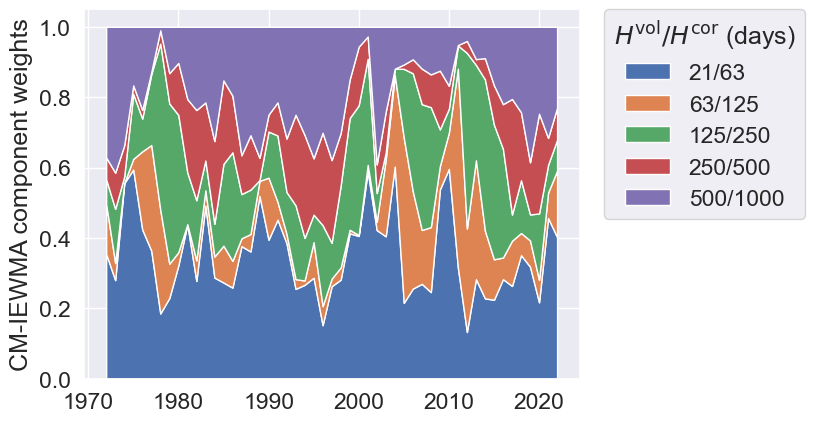
(a) Industry data set.

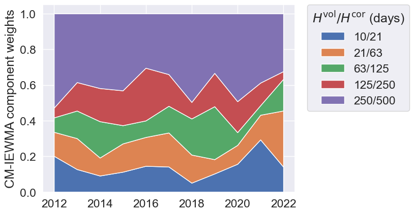
(b) Stock data set.

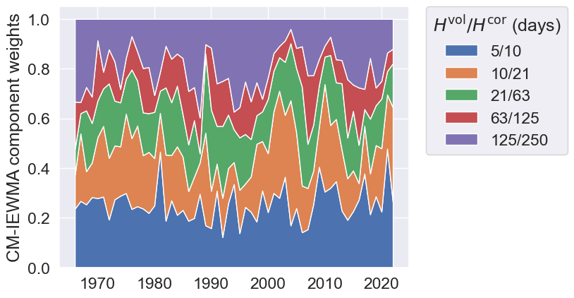
(c) Factor data set.

Figure 6.1: Weights of the various IEWMA components in the CM-IEWMA predictors on three data sets. The IEWMA components are represented as $H^{\text{vol}}/H^{\text{cor}}$ for the volatility and correlation half-lives, respectively.

We can see how the predictor adapts the weights depending on market conditions. Substantial weight is put on the slower (longer half-life) IEWMAs most years. During and following volatile periods like the 2000 dot.com bubble or 2008 market crash, we see a big increase in weight on the faster IEWMAs. We can illustrate these changes in weights in response to market conditions via the effective half-life of the CM-IEWMA, defined as the weighted average of the five (longer) half-lives, shown in figure 6.2, averaged yearly.

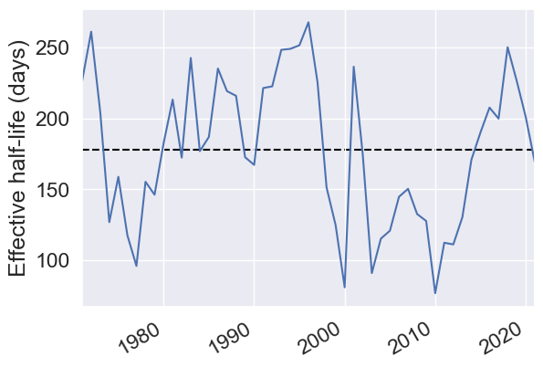
(a) Industry data set.

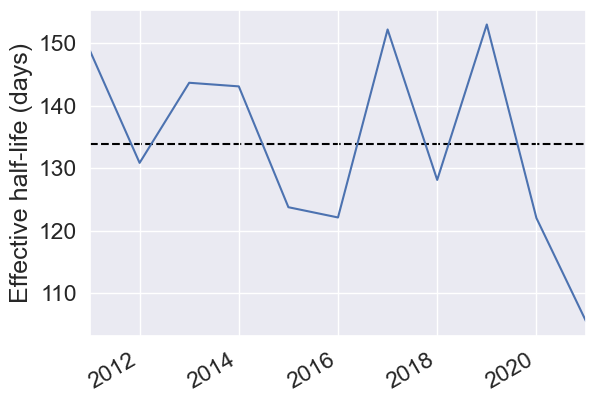
(b) Stock data set.

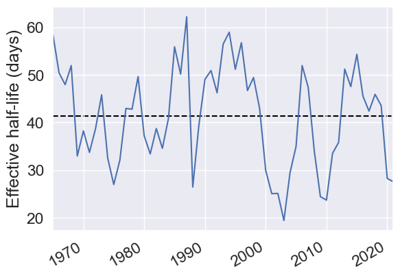
(c) Factor data set.

Figure 6.2: Effective half-lives of the CM-IEWMA predictor on three data sets.

6.2 Mean squared error

Table 6.1 shows the average, standard deviation, and maximum of the MSE computed over distinct quarters for the six covariance predictors on the three data sets (with lower being better for all three metrics).

Table 6.1: Metrics on the MSE, computed over distinct quarters, for six covariance predictors on three data sets.

Predictor	Average/$10^{-4}$	Std. Dev./$10^{-3}$	Max/$10^{-2}$
RW	$7.6$	$4.0$	$3.9$
EWMA	$7.5$	$4.0$	$3.9$
IEWMA	$7.4$	$3.9$	$3.9$
MGARCH	$\mathbf{6.8}$	$\mathbf{3.6}$	$\mathbf{3.8}$
CM-IEWMA	$6.9$	$\mathbf{3.6}$	$\mathbf{3.8}$
Prescient	$6.6$	$3.5$	$3.7$

Industry data set.

Predictor	Average/$10^{-7}$	Std. Dev./$10^{-6}$	Max/$10^{-5}$
RW	$3.4$	$1.9$	$2.4$
EWMA	$3.4$	$1.9$	$2.4$
IEWMA	$3.3$	$1.8$	$2.4$
MGARCH	$\mathbf{3.2}$	$\mathbf{1.8}$	$2.4$
CM-IEWMA	$\mathbf{3.2}$	$\mathbf{1.8}$	$2.4$
Prescient	$3.1$	$1.8$	$2.3$

Stock data set.

Predictor	Average/$10^{-4}$	Std. Dev./$10^{-3}$	Max/$10^{-2}$
RW	$3.4$	$1.6$	$1.1$
EWMA	$3.3$	$1.6$	$1.1$
IEWMA	$3.2$	$1.6$	$1.1$
MGARCH	$3.0$	$\mathbf{1.4}$	$1.0$
CM-IEWMA	$\mathbf{2.9}$	$\mathbf{1.4}$	$\mathbf{0.9}$
Prescient	$3.0$	$1.5$	$1.0$

Factor data set.

CM-IEWMA and MGARCH do better than the other predictors on all metrics over all data sets, with MGARCH doing slightly better on the industry data and CM-IEWMA slightly better on the stock data. Interestingly, on the factor data set, the CM-IEWMA predictor does better than the prescient predictor.

6.3 Log-likelihood and log-likelihood regret

Figure 6.3 shows the average quarterly log-likelihood for the different covariance predictors over the evaluation period. Not surprisingly, the prescient predictor does substantially better than the others. The different predictors follow similar trends, with even the prescient predictor experiencing a drop in log-likelihood during market turbulence. Close inspection shows that the CM-IEWMA and MGARCH predictors almost always have the highest log-likelihood in each quarter.

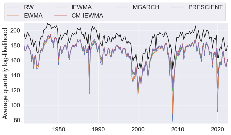
(a) Industry data set.

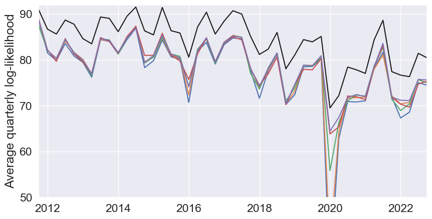
(b) Stock data set.

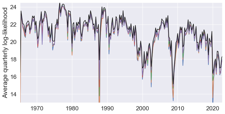
(c) Factor data set.

Figure 6.3: The log-likelihood, averaged quarterly, for six covariance predictors and three data sets.

Figure 6.4 shows the average quarterly log-likelihood regret for the different covariance predictors over the evaluation period. Clearly, CM-IEWMA and MGARCH perform best in volatile markets. Figure 6.5 illustrates the difference between CM-IEWMA and MGARCH. As seen, CM-IEWMA consistently has lower regret on the industry and stock data sets, while they perform similar on the factor data. More precisely, CM-IEWMA has lower regret than MGARCH in 87% of the quarters for the industry data, 71% for the stock data, and 51% for the factor data.

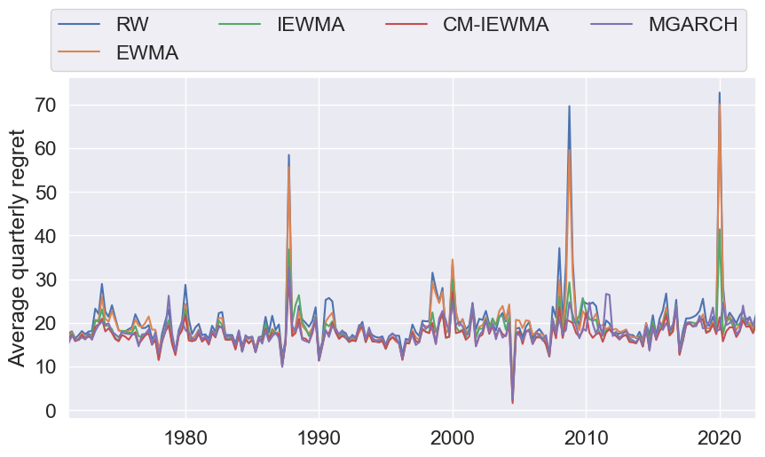
(a) Industry data set.

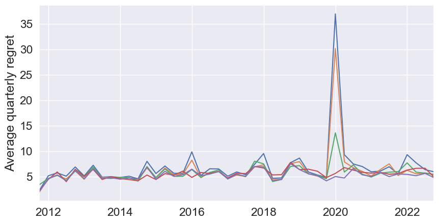
(b) Stock data set.

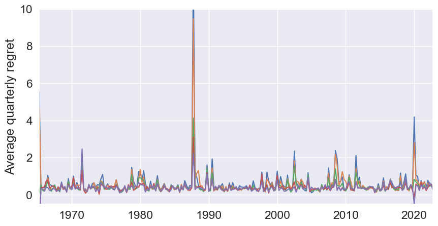
(c) Factor data set.

Figure 6.4: The regret, averaged quarterly, for five covariance predictors over the evaluation periods for three data sets.

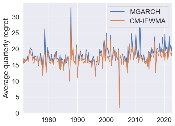
(a) Industry data set.

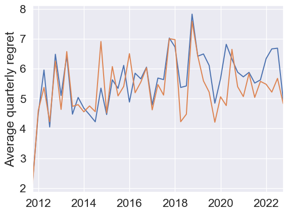
(b) Stock data set.

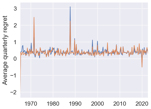
(c) Factor data set.

Figure 6.5: The regret for MGARCH and CM-IEWMA, averaged quarterly over the evaluation periods for three data sets.

Table 6.2: Metrics on the average quarterly regret for six covariance predictors on three data sets.

Predictor	Average	Std. dev.	Max
RW	20.4	6.9	72.8
EWMA	19.4	6.2	70.1
IEWMA	18.2	3.6	41.4
MGARCH	17.9	3.0	32.8
CM-IEWMA	16.9	2.4	28.4
PRESCIENT	0.0	0.0	0.0

Industry data set.

Predictor	Average	Std. dev.	Max
RW	7.0	4.8	37.0
EWMA	6.2	3.8	30.2
IEWMA	5.8	1.6	13.6
MGARCH	5.6	1.0	7.8
CM-IEWMA	5.3	1.0	7.6
PRESCIENT	0.0	0.0	0.0

Stock data set.

Predictor	Average	Std. dev.	Max
RW	0.6	0.9	12.2
EWMA	0.6	0.7	9.5
IEWMA	0.4	0.3	4.1
MGARCH	0.4	0.3	3.1
CM-IEWMA	0.4	0.3	2.9
PRESCIENT	0.0	0.0	0.0

Factor data set.

Table 6.2 illustrates the differences in regret further, by showing the average, standard deviation, and the maximum of the average quarterly regret. As we can see, the average quarterly regret is lower for CM-IEWMA than for the other predictors. The regret is also more stable for CM-IEWMA, as the standard deviation is lower. Finally, the maximum average quarterly regret is also lower for CM-IEWMA than for the other predictors. These results are most prominent on the industry and stock data, while MGARCH does similar on the factor data.

Figure 6.6 gives a final illustration of these results, by showing the cumulative distribution functions of the average quarterly regret for the different covariance predictors.

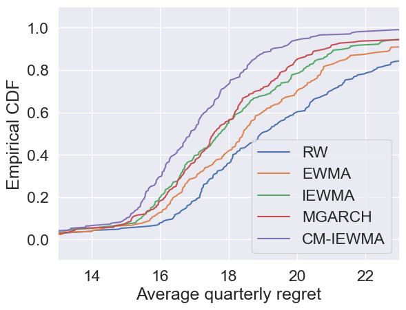
(a) Industry data set.

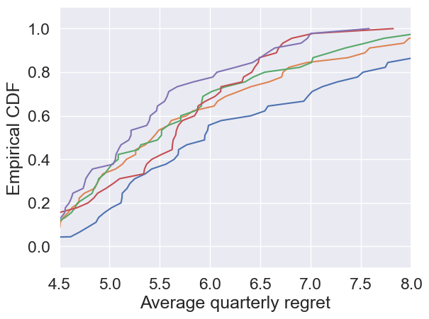
(b) Stock data set.

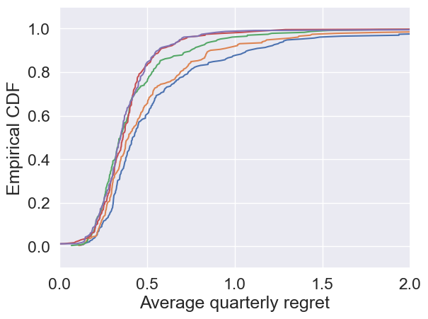
(c) Factor data set.

Figure 6.6: Cumulative distribution functions of average quarterly regret for five covariance predictors on three data sets.

Clearly, CM-IEWMA has the lowest regret on the industry and stock data set, and MGARCH does similar on the factor data.

6.4 Portfolio performance

In this section we evaluate the covariance predictors on the portfolios described in §4.4. In the minimum variance and mean-variance portfolios, we use $L_{\text{max}}=1.6$ (which corresponds to 130:30 long:short), $w_{\text{min}}=-0.1$ and $w_{\text{max}}=0.15$ for the industry and stock return portfolios, and $w_{\text{min}}=-0.3$ and $w_{\text{max}}=0.4$ for the factor return portfolio. We use target (annualized) volatilities of 5%, 10%, and 2% for the industry, stock, and factor return portfolios, respectively.

For the mean-variance portfolio, our estimated returns are EWMAs of the trailing realized returns. For the industry and stock data we use 250-day half-life EWMAs, winsorized at the 40th and 60th percentiles (cross-sectionally), and for the factor data a 63-day half-life EWMA (not winsorized).

Equal weight portfolio.

Table 6.3 shows the metrics for the equal weight portfolio. All predictors track the volatility targets well. MGARCH attains the highest Sharpe ratios, although the results are very close. The drawdowns are also very similar for all predictors, but MGARCH and CM-IEWMA seem slightly better than the rest.

Table 6.3: Metrics for the equal weight portfolio performance for six covariance predictors over the evaluation periods on three data sets.

Predictor	Return/%	Risk/%	Sharpe	Drawdown/%
RW	2.2	5.4	0.4	16
EWMA	2.2	5.1	0.4	15
IEWMA	2.2	5.1	0.4	15
MGARCH	2.4	5.1	0.5	14
CM-IEWMA	2.3	5.0	0.5	13
PRESCIENT	4.3	4.9	0.9	8

Industry data set.

Predictor	Return/%	Risk/%	Sharpe	Drawdown/%
RW	6.8	10.6	0.6	23
EWMA	6.4	10.0	0.6	21
IEWMA	6.7	10.1	0.7	20
MGARCH	7.2	9.4	0.8	15
CM-IEWMA	6.8	9.6	0.7	17
PRESCIENT	12.8	9.9	1.3	10

Stock data set.

Predictor	Return/%	Risk/%	Sharpe	Drawdown/%
RW	2.9	2.1	1.4	15
EWMA	2.9	2.0	1.4	15
IEWMA	3.0	2.0	1.5	14
MGARCH	3.2	2.0	1.6	12
CM-IEWMA	2.9	2.1	1.4	15
PRESCIENT	3.3	2.0	1.7	12

Factor data set.

Minimum variance portfolio.

Table 6.4 shows the metrics for the minimum variance portfolio. For the factor data set, MGARCH does best. On the industry and stock data sets, the three EWMA-based predictors track the volatility target fairly well, while RW and MGARCH underestimate volatility. CM-IEWMA and MGARCH both attain a high Sharpe ratio. However, we note that the high Sharpe ratio for MGARCH, as compared to the other predictors, is a consequence of the high volatility. Finally, CM-IEWMA seems to consistently attain a lower drawdown than the other predictors, although the other EWMA-based approaches also do well.

Table 6.4: Metrics for the minimum variance portfolio performance for six covariance predictors over the evaluation periods on three data sets.

Predictor	Return/%	Risk/%	Sharpe	Drawdown/%
RW	3.1	5.8	0.5	23
EWMA	3.1	5.4	0.6	19
IEWMA	3.3	5.5	0.6	19
MGARCH	4.3	6.1	0.7	20
CM-IEWMA	3.5	5.3	0.7	20
PRESCIENT	3.8	5.0	0.8	13

Industry data set.

Predictor	Return/%	Risk/%	Sharpe	Drawdown/%
RW	9.7	12.0	0.8	23
EWMA	8.9	11.1	0.8	20
IEWMA	9.7	11.3	0.9	19
MGARCH	11.3	12.3	0.9	18
CM-IEWMA	9.1	11.0	0.8	15
PRESCIENT	15.6	10.0	1.6	10

Stock data set.

Predictor	Return/%	Risk/%	Sharpe	Drawdown/%
RW	1.3	2.2	0.6	20
EWMA	1.4	2.1	0.7	18
IEWMA	1.2	2.1	0.6	17
MGARCH	1.8	2.1	0.9	15
CM-IEWMA	1.2	2.1	0.5	21
PRESCIENT	1.0	2.0	0.5	22

Factor data set.

To illustrate how the minimum variance trading strategy has evolved over time, we show the yearly annualized Sharpe ratios for the CM-IEWMA predictor in figure 6.7. We can see that the Sharpe ratio achieved by the minimum variance portfolio decreases over time for the industry and stock data sets, with a small upward trend for the factor data set.

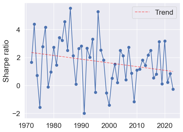
(a) Industry data.

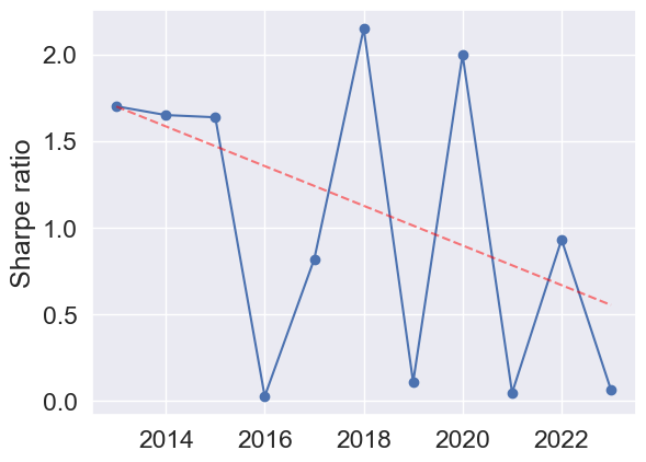
(b) Stock data set.

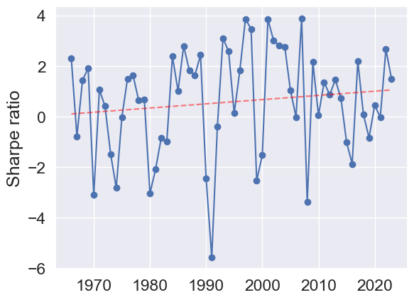
(c) Factor data set.

Figure 6.7: Yearly annualized Sharpe ratios together with the linear trend for minimum variance portfolios on three data sets.

Risk parity portfolio.

The results for the risk-parity portfolio are shown in table 6.5. Overall the results are similar for the various predictors. There is very little that separates the predictors on the industry data set. On the stock data, CM-IEWMA and MGARCH attain the highest Sharpe ratios and lowest drawdowns. On the factor data set, MGARCH has the best overall performance.

Table 6.5: Metrics for the risk parity portfolio performance for six covariance predictors over the evaluation periods on three data sets.

Predictor	Return/%	Risk/%	Sharpe	Drawdown/%
RW	2.4	5.4	0.5	16
EWMA	2.4	5.1	0.5	15
IEWMA	2.5	5.1	0.5	14
MGARCH	2.7	5.1	0.5	14
CM-IEWMA	2.5	5.0	0.5	13
PRESCIENT	4.7	4.9	1.0	8

Industry data set.

Predictor	Return/%	Risk/%	Sharpe	Drawdown/%
RW	7.4	10.8	0.7	22
EWMA	6.8	10.1	0.7	21
IEWMA	7.2	10.2	0.7	20
MGARCH	7.9	9.7	0.8	15
CM-IEWMA	7.4	9.7	0.8	16
PRESCIENT	14.3	9.9	1.5	9

Stock data set.

Predictor	Return/%	Risk/%	Sharpe	Drawdown/%
RW	1.6	2.1	0.7	19
EWMA	1.7	2.1	0.8	18
IEWMA	1.6	2.1	0.8	18
MGARCH	2.0	2.1	1.0	16
CM-IEWMA	1.5	2.1	0.7	17
PRESCIENT	1.4	2.0	0.7	17

Factor data set.

Maximum diversification portfolio.

The maximum diversification portfolio results are illustrated in table 6.6. On the industry and stock data sets, CM-IEWMA and MGARCH do best in terms of Sharpe ratio, drawdown, and tracking the volatility target. On the factor data set, MGARCH does best overall.

Table 6.6: Metrics for the maximum diversification portfolio performance for six covariance predictors over the evaluation periods on three data sets.

Predictor	Return/%	Risk/%	Sharpe	Drawdown/%
RW	2.1	5.5	0.4	16
EWMA	2.1	5.1	0.4	16
IEWMA	2.2	5.2	0.4	14
MGARCH	2.5	5.1	0.5	12
CM-IEWMA	2.3	5.0	0.5	12
PRESCIENT	3.8	5.0	0.8	10

Industry data set.

Predictor	Return/%	Risk/%	Sharpe	Drawdown/%
RW	8.4	11.2	0.8	22
EWMA	7.9	10.4	0.8	21
IEWMA	8.2	10.4	0.8	20
MGARCH	10.0	9.8	1.0	15
CM-IEWMA	8.8	10.0	0.9	16
PRESCIENT	13.5	9.9	1.4	11

Stock data set.

Predictor	Return/%	Risk/%	Sharpe	Drawdown/%
RW	1.4	2.2	0.7	19
EWMA	1.5	2.1	0.7	19
IEWMA	1.4	2.1	0.7	19
MGARCH	2.0	2.1	1.0	16
CM-IEWMA	1.4	2.1	0.7	18
PRESCIENT	1.3	2.0	0.7	18

Factor data set.

Mean variance portfolio.

The results for the mean-variance portfolio are given in table 6.7. On the industry data set all predictors underestimate volatility. The results are similar across predictors, with CM-IEWMA and MGARCH performing slightly better than the rest in terms of Sharpe ratio and drawdown. On the stock data set, CM-IEWMA seems to do best overall. On the factor data set, the results are almost identical between predictors.

Table 6.7: Metrics for the mean variance portfolio performance for six covariance predictors over the evaluation periods on three data sets.

Predictor	Return/%	Risk/%	Sharpe	Drawdown/%
RW	5.6	6.2	0.9	16
EWMA	5.6	5.8	1.0	15
IEWMA	5.9	5.7	1.0	14
MGARCH	6.7	6.4	1.0	14
CM-IEWMA	6.1	5.6	1.1	13
PRESCIENT	4.6	5.0	0.9	10

Industry data set.

Predictor	Return/%	Risk/%	Sharpe	Drawdown/%
RW	6.1	11.9	0.5	26
EWMA	5.9	11.0	0.5	20
IEWMA	7.9	11.1	0.7	15
MGARCH	8.3	11.9	0.7	18
CM-IEWMA	7.3	10.9	0.7	13
PRESCIENT	14.3	9.9	1.4	9

Stock data set.

Predictor	Return/%	Risk/%	Sharpe	Drawdown/%
RW	7.5	2.2	3.3	4
EWMA	7.2	2.1	3.4	4
IEWMA	7.1	2.1	3.3	4
MGARCH	7.3	2.2	3.3	3
CM-IEWMA	6.9	2.2	3.2	4
PRESCIENT	6.5	1.9	3.3	4

Factor data set.

Since we use simple EWMA return predictors, we can expect the mean variance portfolio performance to vary over time. Intuitively it should be better on historical data than more recent data. To illustrate this, figure 6.8 shows the yearly annualized Sharpe ratios for the three portfolios.

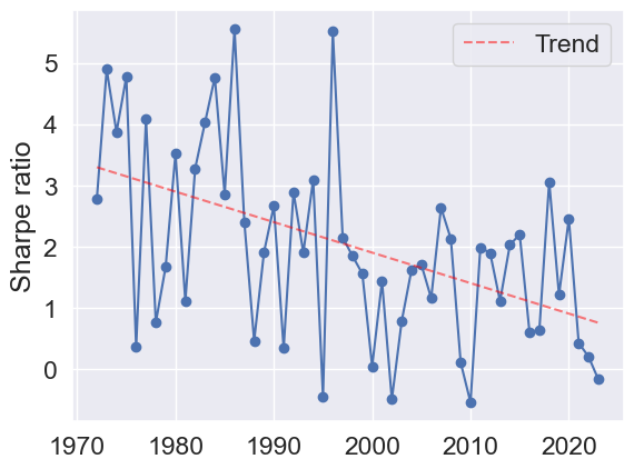
(a) Industry data.

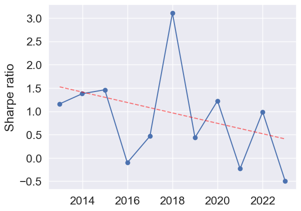
(b) Stock data set.

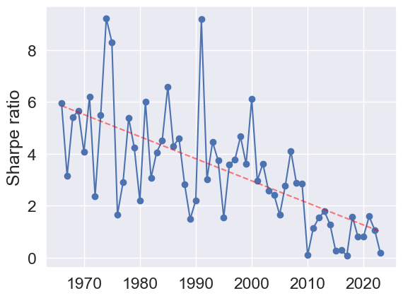
(c) Factor data set.

Figure 6.8: Yearly annualized Sharpe ratios together with the linear trend for mean variance portfolios on three data sets.

There is a clear downward trend in the Sharpe ratios for the industry and factor data sets, illustrating the difficulty of predicting returns in recent years. This can be compared to the minimum variance portfolios (figure 6.7) that have a more stable performance over time, and notably do not depend on a mean estimate.

6.5 Summary

In terms of log-likelihood and regret, CM-IEWMA performs best, followed by MGARCH, which performs better than the simpler covariance predictors. In downstream portfolio optimization experiments, CM-IEWMA and MGARCH again perform better than the other predictors, although in many cases not by much. In these experiments there is more variation in the results, partly explained by the difference between our prediction (of a covariance matrix) and our metrics (such as return, risk, drawdown). Even the simplest covariance predictors do a reasonable job of predicting the portfolio risk.

Chapter 7 Realized covariance

We have so far focused on predicting the covariance matrix of asset returns using historical return data, i.e., we predict $\hat{\Sigma}_{t}$ from $r_{1},\ldots,r_{t-1}$. In this chapter we consider the use of additional data, specifically, intraperiod returns. As an example, suppose the period is (trading) days. The methods described in previous chapters predict the covariance of the daily return from previous daily returns. In so-called realized covariance, we predict the daily return covariance using intraday returns. Instead of single period returns $r_{t}$, we have multiple returns associated with period $t$. It is not surprising that using multiple realized returns for each period, instead of just one, can improve our covariance estimates.

Recent literature has shown that realized volatility and correlation measurements (based on high-frequency intraperiod data) can improve performance over traditional predictors that rely on a single realization per period. hansen2012realized extend the univariate GARCH model to the joint modeling of returns and realized measures of volatility, and show empirically that this improves performance over the standard GARCH model. In [bauwens2012dynamic] a multivariate realized GARCH model is proposed. More recently, [bollerslev2020multivariate] propose a realized semicovariance GARCH model to allow for nuanced responses to positive and negative return shocks.

In this chapter we show that the dynamically weighted prediction combiner of §3.1 readily handles multiple realized returns per period. For simplicity we will assume each period has the same number of intraperiod returns, equally spaced in time. We redefine the return vector to be a return matrix $r_{t}\in{\mbox{\bf R}}^{n\times m}$ with columns that are the $m$ intraperiod return vectors, for times $t=1,\ldots,T$. The realized covariance at time $t$ is defined as

$$C_{t}=r_{t}r_{t}^{T},$$

the same formula for the realized return when $r_{t}$ is a single (vector) return. The realized covariance matrix $C_{t}$ has rank $m$ when the $m$ return vectors are linearly independent and $m\leq n$; this can be compared to the realized covariance when we do not have intraperiod returns, which is rank one.

7.1 Combined multiple realized EWMAs

The dynamically weighted prediction combiner of §3.1 readily handles multiple realized covariance predictors.

Realized EWMA.

We define the realized EWMA (REWMA) predictor as

$$\hat{\Sigma}_{t}=\alpha_{t}\sum_{\tau=1}^{t-1}\beta^{t-1-\tau}C_{\tau},\quad t=2,3,\ldots,$$

where $C_{\tau}$ is the realized covariance at time $\tau$, $\beta\in(0,1)$ is the forgetting factor, and $\alpha_{t}$ is the normalizing constant; see §2.2 for details. This is the same formula as the usual EWMA covariance, with one return per period, given in (2.1), with $r_{t}$ extended to be a matrix of multiple returns.

Combined multiple realized EWMAs.

The combined multiple realized EWMA (CM-REWMA) predictor starts with a set of $K$ REWMA predictors $\hat{\Sigma}_{t}^{(k)}$ with half-lives $H^{(k)}$, $k=1,\ldots,K$, and combines them using the dynamically weighted prediction combiner of §3.1.

7.2 Data and experimental setup

Data set.

We consider a universe of $n=39$ assets with five-minute intraday returns corresponding to $m=77$. The assets were taken as a subset of those used by pelger2020understanding, and are available at [pelger-website]. The data set spans January 2nd 2004 to December 30th 2016, for a total of 252021 data points over 3273 trading days. We list the assets in table 7.1.

Ticker	Company Name
JPM	JPMorgan Chase
GS	Goldman Sachs
KO	The Coca-Cola Company
IBM	International Business Machines Corporation
CAT	Caterpillar Inc.
CVX	Chevron Corporation
XOM	Exxon Mobil Corporation
GE	General Electric Company
MRK	Merck & Co., Inc.
VZ	Verizon Communications Inc.
PFE	Pfizer Inc.
WMT	Walmart Inc.
C	Citigroup Inc.
HD	The Home Depot, Inc.
BA	The Boeing Company
MMM	3M Company
MCD	McDonald’s Corporation
NKE	NIKE, Inc.
JNJ	Johnson & Johnson
INTC	Intel Corporation
MSFT	Microsoft Corporation
AAPL	Apple Inc.
AMZN	Amazon.com Inc.
CSCO	Cisco Systems, Inc.
PG	Procter & Gamble Co.
ABT	Abbott Laboratories
VLO	Valero Energy Corporation
HON	Honeywell International Inc.
LMT	Lockheed Martin Corporation
TXN	Texas Instruments Inc.
COST	Costco Wholesale Corporation
PEP	PepsiCo, Inc.
UNP	Union Pacific Corporation
WFC	Wells Fargo & Co.
CVS	CVS Health Corporation
ORCL	Oracle Corporation
XRX	Xerox Corporation
TMO	Thermo Fisher Scientific Inc.
NSC	Norfolk Southern Corporation

Table 7.1: Assets used in realized covariance study.

Four covariance predictors.

We evaluate four covariance predictors, described below.

• The CM-IEWMA predictor used for the stock data from §5.2. This predictor only uses daily returns, and is not a realized covariance predictor.

• An REWMA predictor with a half-life of $H=10$ days, denoted REWMA-10.

• A CM-REMWA predictor with five components with half-lives of $1,5,10,21$, and $63$ days, respectively.

• Prescient predictor, i.e., the empirical covariance for the quarter the day is in. As with the CM-IEWMA predictor, this predictor uses daily return data. It is of course not implementable, and meant only to show a bound on performance with which to compare our implementable predictors.

7.3 Empirical results

CM-REWMA component weights.

Figure 7.1 shows the component weights for the CM-REWMA predictor, averaged annually.

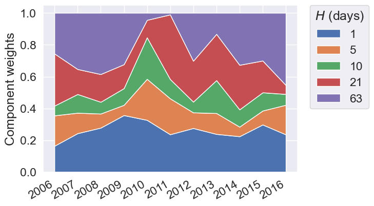
Figure 7.1: CM-REWMA component weights, averaged annually.

The weights are fairly stable over time but a weight shift toward faster changing EWMAs is seen in 2008, during the financial crisis.

MSE.

The average, standard deviation, and maximum MSEs, computed over distinct quarters for the four covariance predictors, are given in table 7.2.

Predictor	Average/$10^{-4}$	Std. Dev./$10^{-3}$	Max/$10^{-3}$
CM-IEWMA	$3.1$	$1.2$	$7.6$
REWMA	$\mathbf{3.0}$	$\mathbf{1.1}$	$7.3$
CM-REWMA	$\mathbf{3.0}$	$\mathbf{1.1}$	$\mathbf{7.2}$
PRESCIENT	$3.0$	$1.1$	$7.1$

Table 7.2: Metrics on the MSE, computed over distinct quarters.

The REWMA and CM-REWMA do slightly better than the CM-IEWMA predictor, but overall there is not a big difference between the predictors.

Regret.

Figure 7.2 shows the average regret over distinct quarters for the CM-IEWMA, REWMA, and CM-REWMA predictors.

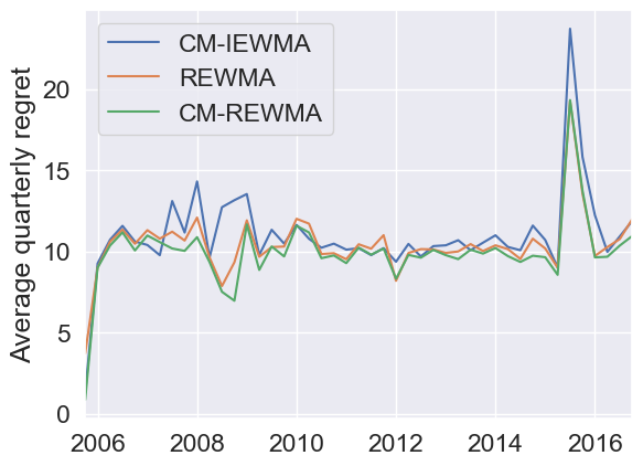
Figure 7.2: Average regret over distinct quarters for three covariance predictors.

The CM-REWMA predictor has the lowest regret in almost all quarters. It has lower regret than the REWMA predictor in 41 out of the 50 quarters, and lower regret than the CM-IEWMA predictor in 39 out of the 50 quarters.

Finally, figure 7.3 shows the cumulative distribution functions of the average quarterly regret for the different covariance predictors.

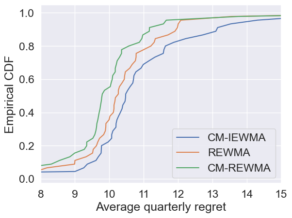
Figure 7.3: Cumulative distribution functions of the average quarterly regret for three covariance predictors.

CM-REWMA has lower regret than both the CM-IEWMA and REWMA predictors, while REWMA has lower regret than CM-IEWMA.

Portfolio performance.

Table 7.3 shows the portfolio metrics for five different portfolio construction methods.

Predictor	Return/%	Risk/%	Sharpe	Drawdown/%
Equal weight
CM-IEWMA	3.2	9.9	0.3	18
REWMA	3.7	10.3	0.4	16
CM-REWMA	4.4	10.6	0.4	16
PRESCIENT	6.7	9.9	0.7	13
Minimum variance
CM-IEWMA	10.7	11.0	1.0	25
REWMA	10.7	10.5	1.0	21
CM-REWMA	12.0	10.7	1.1	21
PRESCIENT	11.7	10.0	1.2	12
Risk parity
CM-IEWMA	4.1	10.0	0.4	18
REWMA	4.7	10.3	0.5	17
CM-REWMA	5.5	10.6	0.5	17
PRESCIENT	8.0	9.9	0.8	12
Maximum diversification
CM-IEWMA	3.6	10.2	0.4	25
REWMA	4.3	10.5	0.4	21
CM-REWMA	5.1	10.8	0.5	19
PRESCIENT	7.8	9.9	0.8	16
Mean variance
CM-IEWMA	8.6	10.5	0.8	22
REWMA	8.5	10.3	0.8	16
CM-REWMA	9.3	10.5	0.9	19
PRESCIENT	10.9	9.8	1.1	21

Table 7.3: Metrics for five different portfolio construction methods, using four covariance predictors.

CM-REWMA does better than, or as well as, REWMA on almost all metrics, and better than CM-IEWMA for all portfolios. However, the difference on portfolio tasks is not large.

Summary.

The results above show that using realized covariance, i.e., intraperiod returns instead of just one return per period, gives covariance estimates that are a bit better than those obtained using only one return per period.

Chapter 8 Large universes

In a practical setting we often encounter a larger number of assets than considered in the previous chapters, which has led to extensive research in high-dimensional covariance estimation. One challenge in large dimensions is ensuring positive definiteness of the covariance matrix, in particular with model-based approaches such as MGARCH [garch_survey]. Several techniques have been proposed for estimating MGARCH models in large dimensions; see, e.g., [engle2019large, de2021factor, de2022large]. Others have focused on estimating realized covariance matrices in high dimensions; see, e.g., [oh2016high, vassallo2021dcc, hautsch2015high, debrito2018forecasting, fan2016incorporating, ait2017using]. For a detailed review of recent developments in high-dimensional covariance estimation, we recommend [bauwens2023modeling, §6].

The methods described in previous chapters can be adapted to handle large universes of assets, say $n$ larger than $100$ or so. In this chapter we describe two closely related methods for improving the performance with large $n$. Both methods end up modeling $\hat{\Sigma}_{t}$ as a low rank plus diagonal matrix, in so-called factor form. Before describing these methods, we mention that evaluating log-likelihood regret is complicated with large $n$. For the empirical covariance to be nonsingular (which is needed to evaluate the regret), we need at least $n$ periods; for daily returns with $n=1000$, this amounts to four years. Even if we have $n$ periods of data, we would only be able to evaluate the regret a few times. For example, with $n=1000$ (four years) we need at least 40 years of data to compute the average regret over 10 distinct periods. The log-likelihood, however, can still be evaluated over fewer than $n$ periods.

8.1 Traditional factor model

In practice most return covariance matrices for large universes are constructed from factors, with the model

$$r_{t}=F_{t}f_{t}+z_{t},\quad t=1,2,\ldots,$$

where $F_{t}\in{\mbox{\bf R}}^{n\times k}$ is the factor exposure matrix, $f_{t}\in{\mbox{\bf R}}^{k}$ is the factor return vector, $z_{t}\in{\mbox{\bf R}}^{n}$ is the idiosyncratic return, and $k$ is the number of factors, typically much smaller than $n$. The factor returns are constructed or found by several methods, such as principal component analysis (PCA), or by hand; see, e.g., [bai2008large, bai2003inferential, lettau2020estimating, lettau2020factors, pelger2022factor, pelger2022interpretable, fama1993common, fama1992cross]. Thus we assume that the factor returns are known. Given the factor returns, the rows of the factor exposure matrix are typically found by least squares regression over a rolling or exponentially weighted window [cochrane2009asset]. The idiosyncratic returns $z_{t}$ are then found as the residuals in this least squares fit. The factor returns $f_{t}$ are modeled as $\mathcal{N}(0,\Sigma_{t}^{\mathrm{f}})$, and the idiosyncratic returns $z_{t}$ are modeled as $\mathcal{N}(0,E_{t})$, where $E_{t}$ is diagonal. It is also assumed that the factor returns and idiosyncratic returns are independent across time and of each other.

We end up with a covariance matrix in factor form, i.e., rank $k$ plus diagonal,

$$\Sigma_{t}=F_{t}\Sigma^{\text{f}}_{t}F_{t}^{T}+{E}_{t}.$$ (8.1)

We can easily use the methods described above with a factor model. Simply predict the factor return covariance $\hat{\Sigma}^{\text{f}}_{t}$ (using the factor returns $f_{t}$) and the idiosyncratic variances $\hat{E}_{t}$ (using the entries of $z_{t}$), using the methods described in this monograph, and then form the covariance estimate

$$\hat{\Sigma}_{t}=F_{t}\hat{\Sigma}^{\text{f}}_{t}F_{t}^{T}+\hat{E}_{t}.$$

The factor model (8.1) can be written in a simpler form as

$$\Sigma_{t}=\tilde{F}_{t}\tilde{F}_{t}^{T}+E_{t},$$ (8.2)

with $\tilde{F}_{t}=F_{t}(\Sigma_{t}^{\text{f}})^{1/2}$. This form does not include a factor covariance $\Sigma^{\text{f}}$, or equivalently, assumes $\Sigma^{\text{f}}_{t}=I$, i.e., the factors are independent with standard deviation one. (The associated factors are called whitened factors.) We will use the factor model form (8.2) in the sequel.

The factor model (8.2) has parameters $\tilde{F}_{t}$ and $E_{t}$, which all together include $nk+n$ scalar parameters. (Some of these are redundant; for example we can insist without loss of generality that $F$ is lower triangular.) The factor model contains substantially fewer scalar parameters than a generic $n\times n$ covariance matrix, which contains $n(n+1)/2$ scalar parameters.

The smaller number of parameters is not the only reason for using a factor model. Another is that it often gives better covariance estimates. We can think of the low rank plus diagonal structure as regularization, which can improve out-of-sample performance. In addition, the low rank plus diagonal structure can be exploited in portfolio construction, bringing the computational complexity down from $O(n^{3})$ to $O(nk^{2})$ operations [boyd2004convex]. This makes portfolio optimization with $n=1000$ assets and $k=50$ factors extremely fast, and makes possible optimization of portfolios with much larger values of $n$.

8.2 Fitting a factor model to a covariance matrix

In this section we consider the problem of fitting a given covariance matrix $\Sigma$ by one in factor form, $\hat{\Sigma}=FF^{T}+E$, where $F\in{\mbox{\bf R}}^{n\times k}$. This corresponds to the model $r=Ff+z$, with (factor return) $f\sim\mathcal{N}(0,I)$, and (idiosyncratic return) $r\sim\mathcal{(}0,E)$, with $E$ diagonal. We let $\theta=(F,E)$ denote the parameters of our factor form model.

We seek $F\in{\mbox{\bf R}}^{n\times k}$ and diagonal $E\in{\mbox{\bf R}}^{n\times n}$ (with positive diagonal entries) that minimize the Kullback-Liebler (KL) divergence between $\mathcal{N}(0,\Sigma)$ and $\mathcal{N}(0,\hat{\Sigma})$,

$$\mathcal{K}(\Sigma,\hat{\Sigma})=\frac{1}{2}\left(\log\frac{\det\hat{\Sigma}}{\det\Sigma}-n+\mathop{\bf Tr}\hat{\Sigma}^{-1}\Sigma\right).$$ (8.3)

The KL divergence can be expressed in terms of the average log-likelihood of $\mathcal{N}(0,\hat{\Sigma})$ under $\mathcal{N}(0,\Sigma)$ as

$$\mathop{\bf E{}}_{r\sim\mathcal{N}(0,\Sigma)}\ell_{\hat{\Sigma}}(r)=-\mathcal{K}(\Sigma,\hat{\Sigma})-(1/2)(n\log 2\pi+n+\log\det\Sigma),$$ (8.4)

where $\ell_{\hat{\Sigma}}(r)$ is the log-likelihood of $r$ under $\mathcal{N}(0,\hat{\Sigma})$. Hence minimizing the KL-divergence (8.3) is equivalent to maximizing the expected log-likelihood (8.4) of $r$ under the model $\mathcal{N}(0,\hat{\Sigma})$.

Solution via EM.

We can use the expectation-maximization (EM) algorithm to approximately minimize $\mathcal{K}(\Sigma,FF^{T}+E)$ over $F$ and $E$ [dempster1977maximum, rubin1982algorithms]. Usually EM is used to fit a factor model to data, i.e., samples; here we use it to fit a given Gaussian distribution $\mathcal{N}(0,\Sigma)$. The method described below was suggested and derived by Emmanuel Cand‘es. We are not aware of its appearance in prior literature. A forthcoming paper on this method will include more detail and applications.

The EM algorithm is an iterative method for maximizing (8.4). Each iteration consists of two steps: the expectation or E-step, and the maximization or M-step. We use the conventional symbols used to describe EM, and use subscript $j=1,2,\ldots$ to denote iteration number. (A good method for initializing the EM algorithm is provided below.)

E-step.

In the E-step, we find the expected log-likelihood under the current estimate of the parameters $\theta_{j}=(F_{j},E_{j})$, over the true distribution of $r$:

$$Q(\theta\,||\,\theta_{j})=\mathop{\bf E{}}_{r\sim\mathcal{N}(0,\Sigma)}\mathop{\bf E{}}_{p_{\theta_{j}}(f\mid r)}\ell_{\theta}(r,f)$$ (8.5)

where $p_{\theta_{j}}(f\mid r)$ is the density of the conditional distribution of $f$ under the parameter estimates at iteration $j$, and $\ell_{\theta}(r,f)$ is the log likelihood of the joint distribution with variable $\theta=(F,E)$.

With our factor model the complete log-likelihood of $(r,f)$ is

$$\ell_{\theta}(r,f) = -\frac{1}{2}\left((r-Ff)^{T}E^{-1}(r-Ff)+f^{T}f+\log\det E\right)$$

$$+\frac{1}{(2\pi)^{n/2}}+\frac{1}{(2\pi)^{k/2}}-k/2.$$

The conditional distribution of $f\mid r$ under $\theta_{j}$ is [bishop2006pattern]

$$f\mid r\leavevmode\nobreak\ \sim\leavevmode\nobreak\ \mathcal{N}(B_{j}r,G_{j}),$$

where

$$B_{j}=G_{j}F_{j}^{T}E_{j}^{-1},\quad G_{j}^{-1}=F_{j}^{T}E_{j}^{-1}F_{j}+I.$$ (8.6)

Hence, (8.5) becomes, up to an additive constant,

$$-\frac{1}{2}\mathop{\bf Tr}(E^{-1}\,(C_{rr}-2C_{rf}F^{T}+FC_{ss}F^{T}))-\frac{1}{2}\log\det E,$$ (8.7)

where

$$C_{rr}=\Sigma,\quad C_{rf}=\Sigma B_{j}^{T},\quad C_{ff}=B_{j}\Sigma B_{j}^{T}+G_{j}.$$ (8.8)

M-step.

In the M-step (8.5) is maximized with respect to $\theta$ to obtain the updated parameters:

$$\theta_{j+1}=\mathop{\rm argmax}_{\theta}\,\,Q(\theta\,||\,\theta_{j}).$$

The maximizer of (8.7) is [rubin1982algorithms]

$${F}_{j+1} = C_{rf}C_{ff}^{-1},$$

$${E}_{j+1} = \mathop{\bf diag}(\mathop{\bf diag}(C_{rr}-2C_{rf}F_{j+1}^{T}+{F}_{j+1}C_{ff}F_{j+1}^{T})),$$

where the inner $\mathop{\bf diag}$ extracts the diagonal of its (matrix) argument, and the outer $\mathop{\bf diag}$ creates a diagonal matrix from its (vector) argument.

EM iteration.

The EM iteration has the form

$${F}_{j+1} = C_{rf}C_{ff}^{-1},$$

$${E}_{j+1} = \mathop{\bf diag}(\mathop{\bf diag}(C_{rr}-2C_{rf}F_{j+1}^{T}+{F}_{j+1}C_{ff}F_{j+1}^{T})),$$

where $C_{rr}$, $C_{rf}$, and $C_{ff}$ come from (8.6) and (8.8).

Initialization.

To initialize the EM algorithm we use the following method, based on low rank approximation via eigendecomposition. We work with the correlation matrix of $\Sigma$, denoted

$$R=\mathop{\bf diag}(\sigma)^{-1}\Sigma\mathop{\bf diag}(\sigma)^{-1},$$

where $\sigma=\mathop{\bf diag}(\Sigma)^{1/2}$ (entrywise). First we express $R$ in its eigendecomposition $R=\sum_{i=1}^{n}\lambda_{i}q_{i}q_{i}^{T}$, with $\lambda_{1}\geq\lambda_{2}\geq\cdots\geq\lambda_{n}$. We then form the rank $k$ approximation

$$\widehat{R}=\sum_{i=1}^{k}\lambda_{i}q_{i}q_{i}^{T}.$$

We only need to compute the $k$ dominant eigenvectors and eigenvalues, which can be done efficiently using for example the Lanczos algorithm [golub2013matrix]. Let

$$\widehat{E}=\mathop{\bf diag}\left(\mathop{\bf diag}(R-\widehat{R})\right),$$

which can be shown to have positive diagonal entries. Our low-rank plus diagonal approximation of $R$ is then $\widehat{R}+\widehat{E}$. It is also a correlation matrix, i.e., has diagonal entries one. Our final factor approximation of $\Sigma$ is given by

$$\mathop{\bf diag}(\sigma)(\widehat{R}+\widehat{E})\mathop{\bf diag}(\sigma)=FF^{T}+E,$$

with

$$F=\mathop{\bf diag}(\sigma)[\sqrt{\lambda_{1}}q_{1}\cdots\sqrt{\lambda_{k}}q_{k}],\qquad E=\mathop{\bf diag}(e\circ\sigma^{2}),$$

where $\circ$ denotes the elementwise (Hadamard) product, and $\sigma^{2}$ means elementwise.

This initialization alone can serve as a basic method to fit a factor model to a given covariance matrix. We will see below that in terms of portfolio optimization, it serves just as well as a factor model fit using the EM method.

8.3 Data and experimental setup

Data set.

We gather the 500 largest NASDAQ stocks (by market capitalization) at the beginning of 2000 from the WRDS portal [WRDS], compute the daily returns of these stocks from January 3rd 2000 to December 30th 2022, and remove any stocks with missing return values during this period. This gives us 238 stocks over 5787 (trading) days. We acknowledge that we induce a survivor bias, but the purpose of this empirical study is solely to demonstrate the benefit of regularization in large universes, and not to backtest a trading strategy.

Traditional factor model.

We create a factor model using PCA as follows. Every year, the $k$ principal components of largest explanatory power are computed, using the past two years of returns. These define the columns of the factor exposure matrix $F_{t}$ for the following year, and the factor returns $f_{t}$ are the projections of the returns onto these principal components. The idiosyncratic returns $z_{t}$ are the residuals. We leverage the CM-IEWMA predictor to compute the factor covariance, using three IEWMA components with half-lives (in days) $H^{\text{vol}}/H^{\text{cor}}$ of $\lceil k/2\rceil/k,k/3k$, and $3k/6k$, where $k$ denotes the number of factors. To estimate the idiosyncratic variances a 21-day EWMA is used. We evaluate the factor models on the average log-likelihood over the evaluation period.

Fitting a factor model to the covariance matrix.

We use a CM-IEWMA covariance predictor with four IEWMA components with half-lives $63/125,125/250,250/500$, and $500/1000$ days, respectively, given as $H^{\text{vol}}/H^{\text{cor}}$. Given the CM-IEWMA estimate $\hat{\Sigma}_{t}$ at time $t$, we approximate it using a factor model as described in §8.2.

To evaluate the factor models, we look at the average log-likelihood over the evaluation period and several performance metrics for a minimum variance portfolio with $L_{\text{max}}=1.6$, $w_{\text{min}}=-0.1$, and $w_{\text{max}}=0.15$, diluted to a target risk of 10%.

8.4 Empirical results

Traditional factor model.

Figure 8.1 shows the log-likelihood versus the number of factors $k$ for $k$ between 2 and 75.

Figure 8.1: Log-likelihood versus the number of factors, using a conventional factor model.

A large increase in log-likelihood is attained with around 20 factors, as compared to using the full covariance matrix. Thus using a traditional factor model and applying our covariance estimation method to the factor returns improves our overall covariance prediction.

Fitting a factor model to the covariance matrix.

Figure 8.2 shows the log-likelihood versus the number of factors (i.e., the rank of the low-rank component) $k$ for various $k$ between 2 and 75, using the eigendecomposition initialization and the EM algorithm.

Figure 8.2: Log-likelihood versus the number of factors, obtained by fitting our covariance estimate with a factor model.

We see that a rank of about $r=20$ seems optimal for this data set, and achieves a noticeably higher log-likelihood than using the full-rank covariance. Moreover, the EM algorithm does better than just computing the eigendecomposition.

Figure 8.3 shows the portfolio metrics for the minimum variance portfolios. We can see that with roughly 10 factors or more, the performance is essentially identical to that obtained using the full covariance matrix. For these experiments we observed no notable difference between the two factor model fitting methods, i.e., the simple eigendecomposition based initialization and the more sophisticated EM method. While using the factor model does not improve portfolio performance, it greatly speeds up the computation of the portfolio optimization problems.

(a) Risk.

(b) Sharpe ratio.

(c) Drawdown.

Figure 8.3: Portfolio metrics for minimum variance portfolios constructed via factor models with various number of factors.

Chapter 9 Smooth covariance predictions

We address here a secondary objective for a covariance prediction $\hat{\Sigma}_{t}$, which is that it vary smoothly across time. Perhaps the main reason for desiring smoothness of the covariance estimate is that it can lead to reduced trading in portfolio construction methods; it can also lead to improved portfolio performance, even without taking into account transaction costs.

To some extent smoothness happens naturally, since whatever method is used to form $\hat{\Sigma}_{t}$ from $r_{1},\ldots,r_{t-1}$ is likely to yield a similar prediction $\hat{\Sigma}_{t+1}$ from $r_{1},\ldots,r_{t}$. It is also possible to further smooth the predictions over time, perhaps trading off some performance, e.g., in log-likelihood regret.

We have already mentioned that the weight optimization problem (3.3) can be modified to encourage smoothness of the weights over time. We can also directly smooth the prediction $\hat{\Sigma}_{t}$, to get a smooth version $\hat{\Sigma}_{t}^{\text{sm}}$. A very simple approach is to let $\hat{\Sigma}_{t}^{\text{sm}}$ be a EWMA of $\hat{\Sigma}_{t}$, with a half-life chosen as a trade-off between smoother predictions and performance. This EWMA post-processing is equivalent to choosing $\hat{\Sigma}_{t}^{\text{sm}}$ to minimize

$$\left\|\hat{\Sigma}_{t}^{\text{sm}}-\hat{\Sigma}_{t}\right\|_{F}^{2}+\lambda\left\|\hat{\Sigma}_{t}^{\text{sm}}-\hat{\Sigma}_{t-1}^{\text{sm}}\right\|_{F}^{2},$$

where $\lambda$ is a positive regularization parameter used to control the trade-off between smoothness and performance, or equivalently, the half-life of the EWMA post-processing. Here the first term is a loss, and the second is a regularizer that encourages smoothly varying covariance predictions.

We can create more sophisticated smoothing methods by changing the loss or the regularizer in this optimization formulation of smoothing. For example we can use the Kullback-Liebler (KL) divergence as a loss. With regularizer $\lambda\|\hat{\Sigma}_{t}^{\text{sm}}-\hat{\Sigma}_{t-1}^{\text{sm}}\|_{F}$ (no square in this case), we obtain a piecewise constant prediction, which roughly speaking only updates the prediction when needed. This is a convex optimization problem which can be solved quickly and reliably [boyd2004convex].

9.1 Data and experimental setup

We consider again the Fama-French factor returns from §5.1, over the same time horizon. We use the CM-IEWMA covariance predictor with the same parameters as in §5.2.

Smoothly varying covariance.

In the first experiment we smooth the CM-IEWMA covariance estimates by applying a EWMA, which corresponds to the $\lambda\left\|\hat{\Sigma}_{t}^{\text{sm}}-\hat{\Sigma}_{t-1}^{\text{sm}}\right\|_{F}^{2}$ regularizer. For different EWMA half-lives we attain different levels of smoothness.

Piecewise constant covariance.

In the second experiment we smooth the CM-IEWMA covariance estimates by applying the $\lambda\left\|\hat{\Sigma}_{t}^{\text{sm}}-\hat{\Sigma}_{t-1}^{\text{sm}}\right\|_{F}$ regularizer. For different values of $\lambda$ we attain piecewise constant covariance predictors with different update frequencies.

9.2 Empirical results

Smoothly varying covariance.

Figure 9.1 shows the regret versus smoothness for various levels of smoothness.

Figure 9.1: Average regret versus smoothness when using EWMA smoothing of the covariance predictor.

As seen, we can reduce the smoothness by a factor of (roughly) four without losing much performance in terms of regret. This can obviously be useful in practice since a smoother covariance estimate would, for example, reduce trading.

Table 9.1 shows the portfolio metrics for various values of $\lambda$ for the minimum variance portfolio with the same parameters as in §6.4; here the turnover is defined as the average of $252\times\|w_{t+1}-w_{t}\|_{1}/\|w_{t}\|_{1}$ over all times $t$ in the evaluation period.

Table 9.1: Portfolio metrics for various EWMA half-lives used for smoothing the covariance. Half-life $0$ means no smoothing.

Half-life/days	Return/%	Risk/%	Sharpe	Drawdown/%	Turnover/%
0	1.2	2.1	0.5	21	$1855$
10	1.4	2.1	0.7	16	$310$
100	1.8	2.1	0.9	15	$56$
250	2.1	2.1	1.0	13	$30$
5000	2.9	2.6	1.1	21	$9$

Interestingly, the right amount of smoothing not only reduces turnover, but also improves portfolio performance in terms of Sharpe ratio and drawdown, while keeping the desired volatility level. Too much smoothing, however, leads to reduced portfolio performance. Figure 9.2 shows the yearly annualized Sharpe ratios for $\lambda=10^{-4}$, indicating a stable performance over time.

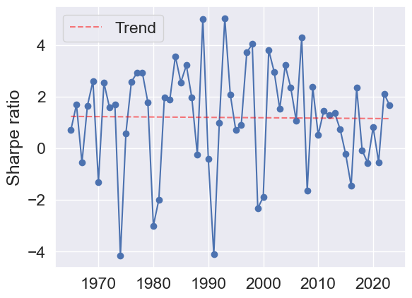
Figure 9.2: Yearly annualized Sharpe ratios for the minimum variance portfolio when smoothing the CM-IEMA covariance predictor with a 250-day half-life EWMA.

Figure 9.3 shows the portfolio weights for three different EWMA half-lives.

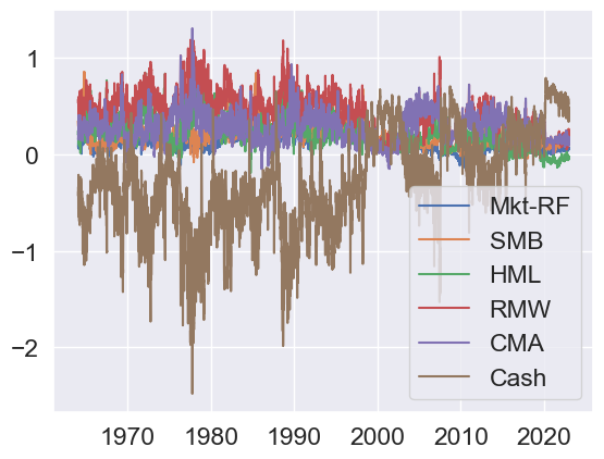
(a) No smoothing.

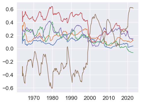
(b) Half-life of 250 days.

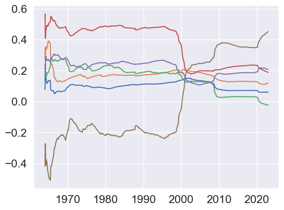
(c) Half-life of 5000 days.

Figure 9.3: Portfolio weights for three different regularization parameters $\lambda$.

As seen, EWMA smoothing leads to smoothly varying portfolio weights, while the weights vary significantly when no smoothing is applied.

Piecewise constant covariance.

Figure 9.4 shows the regret versus the update frequency of the covariance estimate.

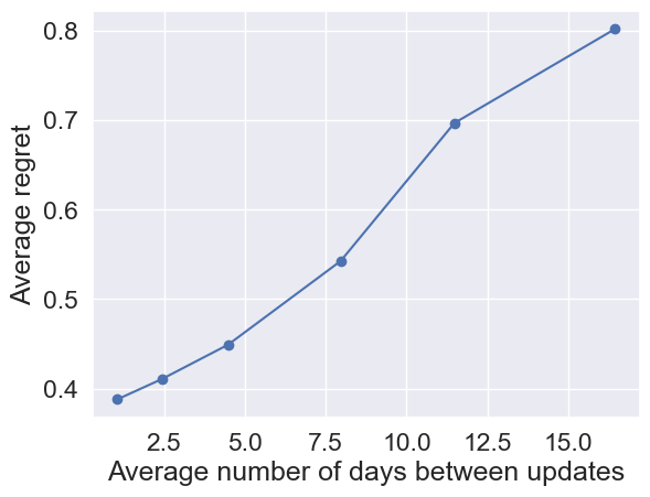
Figure 9.4: Average regret versus time between covariance updates.

There is a clear trade-off between the regret and update frequency. Roughly speaking, we could update the covariance matrix weekly without losing much in terms of regret.

As mentioned, a piecewise constant predictor can be desirable in practice, since it encourages us not updating the portfolio weights, which in turn reduces trading costs. Table 9.2 shows the portfolio metrics for various values of $\lambda$ for the minimum variance portfolio from §6.4.

Table 9.2: Portfolio metrics for various regularization parameters $\lambda$. $\lambda=0$ means no smoothing.

$\lambda$	Return/%	Risk/%	Sharpe	Drawdown/%	Turnover/%
0	1.2	2.1	0.5	21	$1855$
$5\times 10^{-5}$	1.9	2.0	1.0	14	$1190$
$10^{-4}$	2.4	1.9	1.3	9	$112$
$10^{-3}$	2.6	2.1	1.2	17	$7$
$7.5\times 10^{-3}$	3.0	4.8	0.6	31	$0$

As seen, smoothing can significantly reduce turnover, and interestingly improve the Sharpe ratio and drawdown noticeably while maintaining the correct risk level. Figure 9.5 shows the yearly annualized Sharpe ratios for $\lambda=10^{-4}$. The performance is relatively stable over time, with a small downward trend.

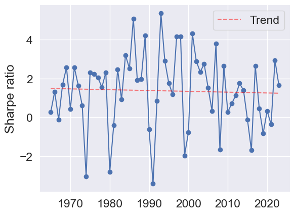
Figure 9.5: Yearly annualized Sharpe ratios for the minimum variance portfolio with a piecewise constant CM-IEMA covariance predictor using $\lambda=10^{-4}$.

To illustrate the impact of smoothing we show the portfolio weights for three different values of $\lambda$ in figure 9.6.

(a) $\lambda=0$.

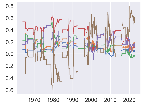
(b) $\lambda=10^{-3}$.

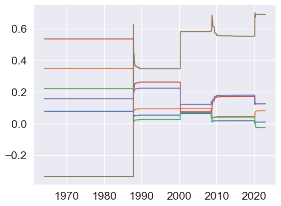
(c) $\lambda=10^{-4}$.

Figure 9.6: Portfolio weights for three different regularization parameters $\lambda$.

Without smoothing the portfolio weights are updated significantly every day. For $\lambda=10^{-4}$ the weights are updated around once or twice a month. Finally, for $\lambda=10^{-5}$ the weights are updated on average every half a year, with only four big weight updates over the whole trading period. Interestingly, the weight updates for $\lambda=10^{-5}$ correspond precisely in time to the volatile regime around 1980, the 2000 dot-com bubble, the 2008 financial crisis, and the 2020 pandemic. In short, we can conclude from table 9.2 and figure 9.6 that smoothing can lead to less trading and improve the portfolio performance.

Finally, we note that there is some deviation between the regret metric and portfolio performance. As seen from figure 9.4 regret increases as we update the covariance matrix less than every other week. However, as seen from table 9.2 and figure 9.6, portfolio performance can improve notably when updating the covariance matrix only every few months, or even years.

Chapter 10 Simulating returns

Our model can be used to simulate future returns, when seeded by past realized ones. To do this, we start with realized returns for periods $1,\ldots,t-1$, and compute $\hat{\Sigma}_{t}$ using our method. Then we generate or sample $r_{t}^{\text{sim}}$ from $\mathcal{N}(0,\hat{\Sigma}_{t})$. We then find $\hat{\Sigma}_{t+1}$ using the returns $r_{1},\ldots,r_{t-1},r^{\text{sim}}_{t}$. We generate $r_{t+1}^{\text{sim}}$ by sampling from $\mathcal{N}(0,\hat{\Sigma}_{t+1})$. This continues.

This simple method generates realistic return data in the short term. Of course, it does not include shocks or rapid changes in the return statistics that we would see in real data, but the generative return method has several practical applications. To mention just one, we can simulate 100 (say) different realizations over the next quarter (say), and use these to compute 100 performance metrics for our portfolio. This gives us a distribution of the performance metric that we might see over the next quarter.

10.1 Data and experimental setup

To illustrate the generative return method, we consider the five Fama-French factor returns from §5.1. Using the same setup as in §5.2 we compute CM-IEMWA covariance estimates, using data from January 1st 2011 to December 31 2013, i.e., over a three-year period. Returns are then generated for 100 days, using the generative mode described above.

10.2 Empirical results

We illustrate the results by looking at the SMB factor, i.e., we look at the marginal distribution of this factor. Figure 10.1 shows the true SMB factor returns and the simulated returns for two different random number generator seeds.

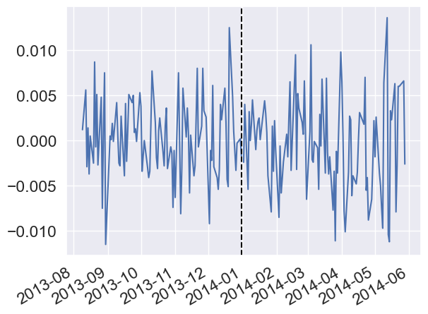
(a) Observed returns.

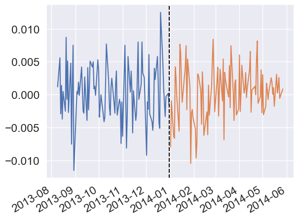
(b) Obeserved returns (left) and simulated returns (right).

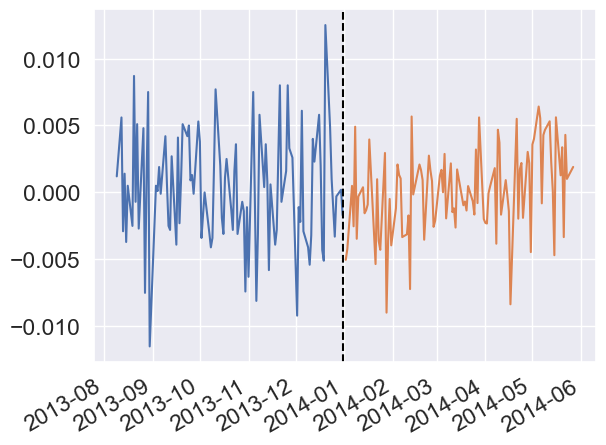
(c) Observed returns (left) and simulated returns (right).

Figure 10.1: Observed and simulated SMB factor returns for two different seeds. The vertical line separates the in-sample (observed returns) and out-of-sample (simulated returns) periods.

As seen, we attain realistic returns that could be used to generate scenarios for downstream portfolio optimization tasks, for example.

Chapter 11 Conclusions

We have introduced a simple method for predicting covariance matrices of financial returns. Our method combines well known ideas such as EWMA, first estimating volatilities and then correlations, and dynamically combining multiple predictions. The method relies on solving a small convex optimization problem (to find the weights used in the combining), which is extremely fast and reliable. The proposed predictor requires little or no tuning or fitting, is interpretable, and produces results better than the popular EWMA estimate, and comparable to MGARCH. Given its interpretability, light weight, and good practical performance, we see it as a practical choice for many applications that require predictions of the covariance of financial returns.