Chain of Log-Concave Markov Chains

Saeed Saremi1, Ji Won Park1, Francis Bach2
1Frontier Research, Prescient Design, Genentech, South San Francisco, CA
2Inria, Ecole Normale Supérieure, Université PSL, Paris, France
Abstract

We introduce a theoretical framework for sampling from unnormalized densities based on a smoothing scheme that uses an isotropic Gaussian kernel with a single fixed noise scale. We prove one can decompose sampling from a density (minimal assumptions made on the density) into a sequence of sampling from log-concave conditional densities via accumulation of noisy measurements with equal noise levels. Our construction is unique in that it keeps track of a history of samples, making it non-Markovian as a whole, but it is lightweight algorithmically as the history only shows up in the form of a running empirical mean of samples. Our sampling algorithm generalizes walk-jump sampling (Saremi & Hyvärinen, 2019). The “walk” phase becomes a (non-Markovian) chain of (log-concave) Markov chains. The “jump” from the accumulated measurements is obtained by empirical Bayes. We study our sampling algorithm quantitatively using the 2-Wasserstein metric and compare it with various Langevin MCMC algorithms. We also report a remarkable capacity of our algorithm to “tunnel” between modes of a distribution.

1 Introduction

Markov chain Monte Carlo (MCMC) is an important class of general-purpose algorithms for sampling from an unnormalized probability density of the form p(x)=ef(x)/Z𝑝𝑥superscript𝑒𝑓𝑥𝑍p(x)=e^{-f(x)}/Z in dsuperscript𝑑\mathbb{R}^{d}. This is a fundamental problem and appears in a variety of fields, e.g., statistical physics going back to 1953 (Metropolis et al., 1953), Bayesian inference (Neal, 1995), and molecular dynamics simulations (Leimkuhler & Matthews, 2015). The biggest challenge facing MCMC is that the distributions of interest lie in very high dimensions and are far from being log-concave, therefore the probability mass is concentrated in small pockets separated by vast empty spaces. These large regions with small probability mass make navigating the space using Markov chains very slow. The second important challenge facing MCMC is that the log-concave pockets themselves are typically ill-conditioned—highly elongated, spanning different directions for different pockets—which only adds to the complexity of sampling.

The framework we develop in this paper aims at addressing these problems. The general philosophy here is that of smoothing, by which we expand the space from dsuperscript𝑑\mathbb{R}^{d} to mdsuperscript𝑚𝑑\mathbb{R}^{md} for some integer m𝑚m and “fill up” the empty space iteratively with probability mass in an approximately isotropic manner, the degree of which we can control using a single smoothing (noise) hyperparameter σ𝜎\sigma. The map from (noisy samples in) mdsuperscript𝑚𝑑\mathbb{R}^{md} back to (clean samples in) dsuperscript𝑑\mathbb{R}^{d} is based on the empirical Bayes formalism (Robbins, 1956; Miyasawa, 1961; Saremi & Hyvärinen, 2019; Saremi & Srivastava, 2022). In essence, a single “jump” using the empirical Bayes estimator removes the masses that were created during sampling. We prove a general result that, for any large m𝑚m, the problem of sampling in dsuperscript𝑑\mathbb{R}^{d} can be reduced to sampling from a sequence of log-concave densities: once log-concave, always log-concave. The trade-off here is the linear time cost of accumulating noisy measurements over m𝑚m iterations.

More formally, instead of sampling from p(x)𝑝𝑥p(x), we sample from the density p(y1:m)𝑝subscript𝑦:1𝑚p(y_{1:m}) that is associated with Y1:m(Y1,,Ym)subscript𝑌:1𝑚subscript𝑌1subscript𝑌𝑚Y_{1:m}\coloneqq(Y_{1},\dots,Y_{m}), where Yt=X+Ntsubscript𝑌𝑡𝑋subscript𝑁𝑡Y_{t}=X+N_{t}, Nt𝒩(0,σ2I)similar-tosubscript𝑁𝑡𝒩0superscript𝜎2𝐼N_{t}\sim\mathcal{N}(0,\sigma^{2}I), all independent for t𝑡t in [m]delimited-[]𝑚[m]. As we show in the paper, there is a duality between sampling from p(x)𝑝𝑥p(x) and sampling from p(y1:m)𝑝subscript𝑦:1𝑚p(y_{1:m}) in the regime where m1/2σsuperscript𝑚12𝜎m^{-1/2}\sigma is small, irrespective of how large σ𝜎\sigma is. This is related to the notion of universality class underlying the smoothed densities. Crucial to our formalism is keeping track of the history of all the noisy samples generated along the way using the factorization

p(y1:m)=p(y1)t=2mp(yt|y1:t1).𝑝subscript𝑦:1𝑚𝑝subscript𝑦1superscriptsubscriptproduct𝑡2𝑚𝑝conditionalsubscript𝑦𝑡subscript𝑦:1𝑡1p(y_{1:m})=p(y_{1})\prod_{t=2}^{m}p(y_{t}|y_{1:t-1}). (1.1)

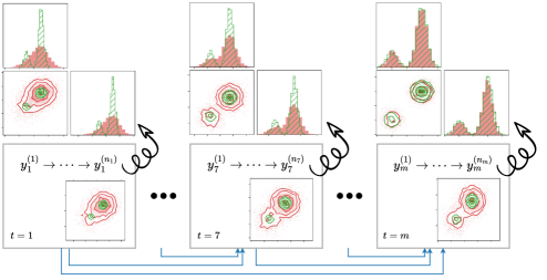
An important element of this sampling scheme is therefore non-Markovian. However, related to our universality results, this history only needs to be tracked in the form of an empirical mean, so the memory footprint is minimal from an algorithmic perspective. See Fig. 1 for a schematic.
Refer to caption
Figure 1: Chain of log-concave Markov chains. Here, (yt(i))i[nt]subscriptsuperscriptsubscript𝑦𝑡𝑖𝑖delimited-[]subscript𝑛𝑡(y_{t}^{(i)})_{i\in[n_{t}]} are samples from a Markov chain, which is used to generate independent draws from p(yt|y1:t1)𝑝conditionalsubscript𝑦𝑡subscript𝑦:1𝑡1p(y_{t}|y_{1:t-1}) for t[m]𝑡delimited-[]𝑚t\in[m]. The blue arrows indicate the non-Markov aspect of our sampling scheme: the accumulation of noisy measurements. The wiggly arrows indicate the denoising “jumps”. In this example, p(yt|y1:t1)𝑝conditionalsubscript𝑦𝑡subscript𝑦:1𝑡1p(y_{t}|y_{1:t-1}) is log-concave for all t𝑡t, but the jumps asymptotically sample the target density (a mixture of two Gaussians) as t𝑡t increases.

A more technical summary of our contributions and the outline of the paper are as follows:

  • In Sec. 2, we prove universality results underlying the smoothed densities p(y1:m)𝑝subscript𝑦:1𝑚p(y_{1:m}).

  • We study anisotropic Gaussians in Sec. 3, proving a negative result regarding the condition number of p(y1:m)𝑝subscript𝑦:1𝑚p(y_{1:m}) in comparison to p(y1)𝑝subscript𝑦1p(y_{1}) in the same universality class. This analysis becomes a segue to our factorization (1.1), where in remarkable contrast we show that the condition number monotonically improves upon accumulation of measurements.

  • Sec. 4 is at the heart of the paper, where we prove several results culminating in Theorem 1, which shows that a broad class of sampling problems can be transformed into a sequence of sampling from strongly log-concave distributions using our measurement accumulation scheme. (This is a feasibility result; in particular, we do not prove here that the log-concave sampling strategy is optimal.) We examine the theorem by algebraically studying an example of a mixture of Gaussians in detail. In Sec. 4, we also outline our general sampling algorithm.

  • We validate our algorithm on carefully designed test densities in Sec. 5. In particular, our algorithm results in lower 2-Wasserstein metric compared to sampling from p(x)𝑝𝑥p(x) using Langevin MCMC (without any smoothing). We also qualitatively report the capacity of our log-concave sampling scheme to tunnel to a mode of a distribution with a small probability mass in a small number of steps when it is initialized at a mode with much higher mass.

1.1 Related Work

Our solution, sketched above, has its roots in walk-jump sampling (Saremi & Hyvärinen, 2019) and its recent generalization (Saremi & Srivastava, 2022). Both papers were framed within the context of generative modeling, i.e., sampling from an unknown distribution from which one has access to independent samples. In contrast, this work lays the theoretical foundation for the fundamental problem of sampling from an unnormalized density when there are no samples available. In addition, regarding the recent development, we show analytically that the intuition expressed by Saremi & Srivastava (2022) regarding the distribution p(y1:m)𝑝subscript𝑦:1𝑚p(y_{1:m}) being well-conditioned is not correct. This nontrivial negative result motivates our analysis of the non-Markovian scheme for sampling p(y1:m)𝑝subscript𝑦:1𝑚p(y_{1:m}).

Our methodology is agnostic to the algorithm used for sampling from p(yt|y1:t1)𝑝conditionalsubscript𝑦𝑡subscript𝑦:1𝑡1p(y_{t}|y_{1:t-1}) in (1.1). However, we have been particularly motivated by the research on Langevin MCMC which is a class of gradient-based sampling algorithms obtained by discretizing the Langevin diffusion (Parisi, 1981). There is a growing body of work on the analysis of Langevin MCMC algorithms of various complexity (overdampled, Metropolis-adjusted, underdamped, higher-order) for sampling from log-concave distributions (Dalalyan, 2017; Durmus & Moulines, 2017; Cheng et al., 2018; Dwivedi et al., 2018; Shen & Lee, 2019; Cao et al., 2020; Mou et al., 2021; Li et al., 2022). In our experiments, we compare several recent Langevin MCMC methods, which may be of independent interest.

There is a significant body of work on sequential methods for sampling, rooted in annealing methods in optimization (Kirkpatrick et al., 1983), which became popular in the MCMC literature due to Neal’s seminal paper on annealed importance sampling (Neal, 2001). Diffusion models (Sohl-Dickstein et al., 2015; Ho et al., 2020) are a related class of sequential methods for generative modeling. Our sequential scheme is distinguished from earlier methods from separate angles: (I) Although we sample the conditional densities with Markov chains, we condition on all the previous samples that were generated. As a whole, our scheme is strictly non-Markovian. (II) In our sequential scheme, we are able to guarantee that we sample from (progressively more) log-concave densities. To our knowledge, no other sampling frameworks can make such guarantees. (III) Compared to diffusion models, the noise level in our framework is held fixed. This is an important feature of our sampling algorithm and it underlies many of its theoretical properties. (IV) All prior sequential schemes rely on a noising/annealing schedule which is hard to tune, and their performance is sensitive to the choice of the schedule (Karras et al., 2022; Syed et al., 2022). In contrast, our sequential scheme is free of scheduling and relies on only two parameters: the noise level σ𝜎\sigma and the number of measurements m𝑚m.

Notation.

We use p𝑝p to denote probability density functions and adopt the convention where we drop the random variable subscript to p𝑝p when the arguments are present, e.g., p(x)pX(x)𝑝𝑥subscript𝑝𝑋𝑥p(x)\coloneqq p_{X}(x), p(y2|y1)pY2|Y1=y1(y2)𝑝conditionalsubscript𝑦2subscript𝑦1subscript𝑝conditionalsubscript𝑌2subscript𝑌1subscript𝑦1subscript𝑦2p(y_{2}|y_{1})\coloneqq p_{Y_{2}|Y_{1}=y_{1}}(y_{2}). We reserve f𝑓f to be the energy function associated with p(x)ef(x)proportional-to𝑝𝑥superscript𝑒𝑓𝑥p(x)\propto e^{-f(x)}. We use λ𝜆\lambda to denote the spectrum of a matrix, e.g., λmax(C)subscript𝜆𝐶\lambda_{\max}(C) is the largest eigenvalue of C𝐶C. We use the shorthand notations [m]={1,,m}delimited-[]𝑚1𝑚[m]=\{1,\dots,m\}, y1:m=(y1,,ym)subscript𝑦:1𝑚subscript𝑦1subscript𝑦𝑚y_{1:m}=(y_{1},\dots,y_{m}), and y¯1:m=1mt=1mytsubscript¯𝑦:1𝑚1𝑚superscriptsubscript𝑡1𝑚subscript𝑦𝑡\overline{y}_{1:m}=\frac{1}{m}\sum_{t=1}^{m}y_{t}.

2 Universal (σ,m)𝜎𝑚(\sigma,m)-densities

Consider the multimeasurement (factorial kernel) generalization of the kernel density by Saremi & Srivastava (2022) for m𝑚m isotropic Gaussian kernels with equal noise level (kernel bandwidth) σ𝜎\sigma:

p(y1:m)def(x)exp(12σ2t=1mxyt2)𝑑x.proportional-to𝑝subscript𝑦:1𝑚subscriptsuperscript𝑑superscript𝑒𝑓𝑥12superscript𝜎2superscriptsubscript𝑡1𝑚superscriptnorm𝑥subscript𝑦𝑡2differential-d𝑥p(y_{1:m})\propto\int_{\mathbb{R}^{d}}e^{-f(x)}\exp\Bigl{(}-\frac{1}{2\sigma^{2}}\sum_{t=1}^{m}{\big{\|}}x-y_{t}{\big{\|}}^{2}\Bigr{)}dx. (2.1)

We refer to p(y1:m)𝑝subscript𝑦:1𝑚p(y_{1:m}) as the (σ,m)𝜎𝑚(\sigma,m)-density. Equivalently, Yt|x𝒩(x,σ2I)similar-toconditionalsubscript𝑌𝑡𝑥𝒩𝑥superscript𝜎2𝐼Y_{t}|x\sim\mathcal{N}(x,\sigma^{2}I), t[m]𝑡delimited-[]𝑚t\in[m] all independent. Clearly, p(y1:m)𝑝subscript𝑦:1𝑚p(y_{1:m}) is permutation invariant p(y1,,ym)=p(yπ(1),,yπ(m)),𝑝subscript𝑦1subscript𝑦𝑚𝑝subscript𝑦𝜋1subscript𝑦𝜋𝑚p(y_{1},\dots,y_{m})=p(y_{\pi(1)},\dots,y_{\pi(m)}), where π:[m][m]:𝜋delimited-[]𝑚delimited-[]𝑚\pi:[m]\rightarrow[m] is a permutation of the m𝑚m measurements. We set the stage for the remainder of the paper with a calculation that shows the permutation invariance takes the following form (see Appendix A):

logp(y1:m)=φ(y¯1:m;m1/2σ)+m2σ2(y¯1:m21mt=1myt2)+cst,𝑝subscript𝑦:1𝑚𝜑subscript¯𝑦:1𝑚superscript𝑚12𝜎𝑚2superscript𝜎2superscriptnormsubscript¯𝑦:1𝑚21𝑚superscriptsubscript𝑡1𝑚superscriptnormsubscript𝑦𝑡2cst\log p(y_{1:m})=\varphi(\overline{y}_{1:m};m^{-1/2}\sigma)+\frac{m}{2\sigma^{2}}\Bigl{(}\|\overline{y}_{1:m}\|^{2}-\frac{1}{m}\sum_{t=1}^{m}\|y_{t}\|^{2}\Bigr{)}+{{\rm cst}}, (2.2)

where

φ(y;σ)log𝔼x𝒩(y,σ2I)[ef(x)].𝜑𝑦𝜎subscript𝔼similar-to𝑥𝒩𝑦superscript𝜎2𝐼delimited-[]superscript𝑒𝑓𝑥\varphi(y;\sigma)\coloneqq\log\mathbb{E}_{x\sim\mathcal{N}(y,\sigma^{2}I)}[e^{-f(x)}].

The calculation is straightforward by grouping the sums of squares in (2.1):

t=1mxyt2=m(xy¯1:m2+y¯1:m21mt=1myt2)+cst.superscriptsubscript𝑡1𝑚superscriptnorm𝑥subscript𝑦𝑡2𝑚superscriptnorm𝑥subscript¯𝑦:1𝑚2superscriptnormsubscript¯𝑦:1𝑚21𝑚superscriptsubscript𝑡1𝑚superscriptnormsubscript𝑦𝑡2cst-\sum_{t=1}^{m}\|x-y_{t}\|^{2}=m\Bigl{(}-\|x-\overline{y}_{1:m}\|^{2}+\|\overline{y}_{1:m}\|^{2}-\frac{1}{m}\sum_{t=1}^{m}\|y_{t}\|^{2}\Bigr{)}+{{\rm cst}}.

In addition, the Bayes estimator of X𝑋X given Y1:m=y1:msubscript𝑌:1𝑚subscript𝑦:1𝑚Y_{1:m}=y_{1:m} simplifies as follows (see Appendix A):

𝔼[X|y1:m]=y¯1:m+m1σ2φ(y¯1:m;m1/2σ).𝔼delimited-[]conditional𝑋subscript𝑦:1𝑚subscript¯𝑦:1𝑚superscript𝑚1superscript𝜎2𝜑subscript¯𝑦:1𝑚superscript𝑚12𝜎\mathbb{E}[X|y_{1:m}]=\overline{y}_{1:m}+m^{-1}\sigma^{2}\nabla\varphi(\overline{y}_{1:m};m^{-1/2}\sigma). (2.3)

These calculations bring out a notion of universality class that is associated with p(y1:m)𝑝subscript𝑦:1𝑚p(y_{1:m}) formalized by the following definition and proposition.

Definition 1 (Universality Class).

We define the universality class [σ~]delimited-[]~𝜎[\tilde{\sigma}] as the set of densities p(y1:m)𝑝subscript𝑦:1𝑚p(y_{1:m}), in the family of (σ,m)𝜎𝑚(\sigma,m)-densities, such that for all (σ,m)[σ~]𝜎𝑚delimited-[]~𝜎(\sigma,m)\in[\tilde{\sigma}] the following holds: m1/2σ=σ~.superscript𝑚12𝜎~𝜎m^{-1/2}\sigma=\tilde{\sigma}.

Proposition 1.

If Y1:mp(y1:m)similar-tosubscript𝑌:1𝑚𝑝subscript𝑦:1𝑚Y_{1:m}\sim p(y_{1:m}), let p^σ,msubscript^𝑝𝜎𝑚\hat{p}_{\sigma,m} be the distribution of 𝔼[X|Y1:m]𝔼delimited-[]conditional𝑋subscript𝑌:1𝑚\mathbb{E}[X|Y_{1:m}], and define p^σ=p^σ,1subscript^𝑝𝜎subscript^𝑝𝜎1\hat{p}_{\sigma}=\hat{p}_{\sigma,1}. Then p^σ,m=p^m1/2σsubscript^𝑝𝜎𝑚subscript^𝑝superscript𝑚12𝜎\hat{p}_{\sigma,m}=\hat{p}_{m^{-1/2}\sigma}. In other words, p^σ,msubscript^𝑝𝜎𝑚\hat{p}_{\sigma,m} is identical for densities in the same universality class.

Proof.

We are given Xef(x)similar-to𝑋superscript𝑒𝑓𝑥X\sim e^{-f(x)}, Yt=X+εtsubscript𝑌𝑡𝑋subscript𝜀𝑡Y_{t}=X+\varepsilon_{t}, εt𝒩(0,σ2I)similar-tosubscript𝜀𝑡𝒩0superscript𝜎2𝐼\varepsilon_{t}\sim\mathcal{N}(0,\sigma^{2}I) independently for t[m]𝑡delimited-[]𝑚t\in[m]. It follows Y¯1:m=X+ε~subscript¯𝑌:1𝑚𝑋~𝜀\overline{Y}_{1:m}=X+\tilde{\varepsilon}, where ε~𝒩(0,σ~2I)similar-to~𝜀𝒩0superscript~𝜎2𝐼\tilde{\varepsilon}\sim\mathcal{N}(0,\tilde{\sigma}^{2}I), where σ~2=m1σ2superscript~𝜎2superscript𝑚1superscript𝜎2\tilde{\sigma}^{2}=m^{-1}\sigma^{2}. Using (2.3), 𝔼[X|y1:m]𝔼delimited-[]conditional𝑋subscript𝑦:1𝑚\mathbb{E}[X|y_{1:m}] is distributed as

X+ε~+σ~2φ(X+ε~;σ~),𝑋~𝜀superscript~𝜎2𝜑𝑋~𝜀~𝜎X+\tilde{\varepsilon}+\tilde{\sigma}^{2}\nabla\varphi(X+\tilde{\varepsilon};\tilde{\sigma}),

which is identical for all densities p(y1:m)𝑝subscript𝑦:1𝑚p(y_{1:m}) in [σ~]delimited-[]~𝜎[\tilde{\sigma}]. ∎

2.1 Distribution of 𝔼[X|y1:m]𝔼delimited-[]conditional𝑋subscript𝑦:1𝑚\mathbb{E}[X|y_{1:m}] vs. pXsubscript𝑝𝑋p_{X}: upper bound on the 2-Wasserstein distance

Our goal is to obtain samples from pXsubscript𝑝𝑋p_{X}, but in walk-jump sampling the samples are given by 𝔼[X|y1:m]𝔼delimited-[]conditional𝑋subscript𝑦:1𝑚\mathbb{E}[X|y_{1:m}], where y1:mp(y1:m)similar-tosubscript𝑦:1𝑚𝑝subscript𝑦:1𝑚y_{1:m}\sim p(y_{1:m}) (Saremi & Hyvärinen, 2019; Saremi & Srivastava, 2022). Next, we address how far p^σ,msubscript^𝑝𝜎𝑚\hat{p}_{\sigma,m} is from the density of interest pXsubscript𝑝𝑋p_{X}.

Proposition 2.

The squared 2-Wasserstein distance between pXsubscript𝑝𝑋p_{X} and p^σ,msubscript^𝑝𝜎𝑚\hat{p}_{\sigma,m} is bounded by

W2(pX,p^σ,m)2σ2md.subscript𝑊2superscriptsubscript𝑝𝑋subscript^𝑝𝜎𝑚2superscript𝜎2𝑚𝑑W_{2}(p_{X},\hat{p}_{\sigma,m})^{2}\leqslant\frac{\sigma^{2}}{m}d.

The proof is given in Appendix B. As expected, the upper bound is expressed in terms of σ~2=σ2/m.superscript~𝜎2superscript𝜎2𝑚\tilde{\sigma}^{2}=\sigma^{2}/m. A close inspection of the proof shows that the bound above is loose as it is obtained from the rate resulting from replacing the empirical Bayes estimator 𝔼[X|y1:m]𝔼delimited-[]conditional𝑋subscript𝑦:1𝑚\mathbb{E}[X|y_{1:m}] with the empirical mean Y¯1:msubscript¯𝑌:1𝑚\overline{Y}_{1:m}. Note, however, that when the prior p(x)𝑝𝑥p(x) is “strong” (e.g., low entropy), the dependence on σ2/msuperscript𝜎2𝑚\sigma^{2}/m can be significantly improved.

3 The geometry of (σ,m)𝜎𝑚(\sigma,m)-densities

In this section we analyze at the problem of sampling from p(y1:m)𝑝subscript𝑦:1𝑚p(y_{1:m}) where we consider p(x)𝑝𝑥p(x) to be an anisotropic Gaussian, X𝒩(0,C)similar-to𝑋𝒩0𝐶X\sim\mathcal{N}(0,C), with a diagonal covariance matrix:

C=diag(τ12,,τd2).𝐶diagsuperscriptsubscript𝜏12superscriptsubscript𝜏𝑑2C={\rm diag}(\tau_{1}^{2},\dots,\tau_{d}^{2}). (3.1)

The density pXsubscript𝑝𝑋p_{X} is strongly log-concave with the property τmax2I2f(x)τmin2Iprecedes-or-equalssuperscriptsubscript𝜏2𝐼superscript2𝑓𝑥precedes-or-equalssuperscriptsubscript𝜏2𝐼\tau_{\max}^{-2}I\preccurlyeq\nabla^{2}f(x)\preccurlyeq\tau_{\min}^{-2}I, therefore its condition number is κ=τmin2τmax2𝜅superscriptsubscript𝜏2superscriptsubscript𝜏2\kappa=\tau_{\min}^{-2}\tau_{\max}^{2}. Log-concave densities with κ1much-greater-than𝜅1\kappa\gg 1 are considered ill-conditioned. Since Y1𝒩(0,C+σ2I)similar-tosubscript𝑌1𝒩0𝐶superscript𝜎2𝐼Y_{1}\sim\mathcal{N}(0,C+\sigma^{2}I), the condition number for (single-measurement) smoothed density, which we denote by κσ,1subscript𝜅𝜎1\kappa_{\sigma,1} is given by:

κσ,1=(1+σ2τmax2)/(1+σ2τmin2).subscript𝜅𝜎11superscript𝜎2superscriptsubscript𝜏21superscript𝜎2superscriptsubscript𝜏2\kappa_{\sigma,1}=(1+\sigma^{-2}\tau_{\max}^{2})/(1+\sigma^{-2}\tau_{\min}^{2}). (3.2)

Next, we give the full spectrum of the precision matrix associated with (σ,m)𝜎𝑚(\sigma,m)-densities.

Proposition 3.

Consider an anisotropic Gaussian density X𝒩(0,C)similar-to𝑋𝒩0𝐶X\sim\mathcal{N}(0,C) in dsuperscript𝑑\mathbb{R}^{d}, where Cij=τi2δijsubscript𝐶𝑖𝑗superscriptsubscript𝜏𝑖2subscript𝛿𝑖𝑗C_{ij}=\tau_{i}^{2}\delta_{ij}. Then the (σ,m)𝜎𝑚(\sigma,m)-density is a centered Gaussian in mdsuperscript𝑚𝑑\mathbb{R}^{md}: Y1:m𝒩(0,Fσ,m1)similar-tosubscript𝑌:1𝑚𝒩0superscriptsubscript𝐹𝜎𝑚1Y_{1:m}\sim\mathcal{N}(0,F_{\sigma,m}^{-1}). For m2𝑚2m\geqslant 2, the precision matrix Fσ,msubscript𝐹𝜎𝑚F_{\sigma,m} is block diagonal with d𝑑d blocks (indexed by i𝑖i) of size m×m𝑚𝑚m\times m, each with the following spectrum: (i) There are m1𝑚1m-1 degenerate eigenvalues equal to σ2,superscript𝜎2\sigma^{-2}, (ii) The remaining eigenvalue equals to (σ2+mτi2)1.superscriptsuperscript𝜎2𝑚superscriptsubscript𝜏𝑖21(\sigma^{2}+m\tau_{i}^{2})^{-1}. The condition number κσ,msubscript𝜅𝜎𝑚\kappa_{\sigma,m} associated with the (σ,m)𝜎𝑚(\sigma,m)-density is given by:

κσ,m=λmax(Fσ,m)λmin(Fσ,m)=1+mσ2τmax2.subscript𝜅𝜎𝑚subscript𝜆maxsubscript𝐹𝜎𝑚subscript𝜆minsubscript𝐹𝜎𝑚1𝑚superscript𝜎2superscriptsubscript𝜏max2\kappa_{\sigma,m}=\frac{\lambda_{\rm max}(F_{\sigma,m})}{\lambda_{\rm min}(F_{\sigma,m})}=1+m\cdot\sigma^{-2}\tau_{\rm max}^{2}.
Remark 1 (The curse of sampling all measurements at once).

The above proposition is a negative result regarding sampling from p(y1:m)𝑝subscript𝑦:1𝑚p(y_{1:m}) if—this is an important “if”—all m𝑚m measurements y1:msubscript𝑦:1𝑚y_{1:m} are sampled in parallel (at the same time). This is because mσ2=σ~2𝑚superscript𝜎2superscript~𝜎2m\sigma^{-2}=\tilde{\sigma}^{-2} remains constant for m>1𝑚1m>1 for (σ,m)[σ~]𝜎𝑚delimited-[]~𝜎(\sigma,m)\in[\tilde{\sigma}]—even worse, the condition number κσ,msubscript𝜅𝜎𝑚\kappa_{\sigma,m} is strictly greater than κσ~,1subscript𝜅~𝜎1\kappa_{\tilde{\sigma},1} for m>1𝑚1m>1.

This negative result regarding the sampling scheme by Saremi & Srivastava (2022), we call all (measurements) at once (AAO), leads to our investigation below into sampling from p(y1:m)𝑝subscript𝑦:1𝑚p(y_{1:m}) sequentially, one (measurement) at a time (OAT), by accumulating measurements using the factorization (1.1). Now, we perform the analysis in Proposition 3 for the spectrum of the conditional densities in (1.1).

Proposition 4.

Assume X𝒩(0,C)similar-to𝑋𝒩0𝐶X\sim\mathcal{N}(0,C) is the anisotropic Gaussian in Proposition 3. Given the factorization of p(y1:m)𝑝subscript𝑦:1𝑚p(y_{1:m}) in (1.1), for t>1𝑡1t>1, the conditional density p(yt|y1:t1)𝑝conditionalsubscript𝑦𝑡subscript𝑦:1𝑡1p(y_{t}|y_{1:t-1}) is a Gaussian with a shifted mean, and with a diagonal covariance matrix:

2σ2logp(yt|y1:t1)=i=1d(1Ati)(ytiAti1Atik=1t1yki)2+cst,2superscript𝜎2𝑝conditionalsubscript𝑦𝑡subscript𝑦:1𝑡1superscriptsubscript𝑖1𝑑1subscript𝐴𝑡𝑖superscriptsubscript𝑦𝑡𝑖subscript𝐴𝑡𝑖1subscript𝐴𝑡𝑖superscriptsubscript𝑘1𝑡1subscript𝑦𝑘𝑖2cst-2\sigma^{2}\log p(y_{t}|y_{1:t-1})=\sum_{i=1}^{d}\left(1-A_{ti}\right)\cdot\Bigl{(}y_{ti}-\frac{A_{ti}}{1-A_{ti}}\sum_{k=1}^{t-1}y_{ki}\Bigr{)}^{2}+{{\rm cst}},

where Atisubscript𝐴𝑡𝑖A_{ti} is short for Ati=(t+σ2τi2)1subscript𝐴𝑡𝑖superscript𝑡superscript𝜎2superscriptsubscript𝜏𝑖21A_{ti}=\left(t+\sigma^{2}\tau_{i}^{-2}\right)^{-1}. The precision matrix associated with p(yt|y1:t1)𝑝conditionalsubscript𝑦𝑡subscript𝑦:1𝑡1p(y_{t}|y_{1:t-1}), denoted by Ft|1:t1subscript𝐹:conditional𝑡1𝑡1F_{t|1:t-1}, has the following spectrum

σ2λi(Ft|1:t1)=1(t+σ2τi2)1,superscript𝜎2subscript𝜆𝑖subscript𝐹:conditional𝑡1𝑡11superscript𝑡superscript𝜎2superscriptsubscript𝜏𝑖21\sigma^{2}\lambda_{i}(F_{t|1:t-1})=1-\left(t+\sigma^{2}\tau_{i}^{-2}\right)^{-1},

with the following condition number

κt|1:t1=1(t+σ2τmin2)11(t+σ2τmax2)1.subscript𝜅:conditional𝑡1𝑡11superscript𝑡superscript𝜎2superscriptsubscript𝜏211superscript𝑡superscript𝜎2superscriptsubscript𝜏21\kappa_{t|1:t-1}=\frac{1-(t+\sigma^{2}\tau_{\min}^{-2})^{-1}}{1-(t+\sigma^{2}\tau_{\max}^{-2})^{-1}}.

Lastly, the condition number κt|1:t1subscript𝜅:conditional𝑡1𝑡1\kappa_{t|1:t-1} is monotonically decreasing as t𝑡t increases (for any m>1𝑚1m>1):

1<κm|1:m1<<κ3|1:2<κ2|1<κ1,1subscript𝜅:conditional𝑚1𝑚1subscript𝜅:conditional312subscript𝜅conditional21subscript𝜅11<\kappa_{m|1:m-1}<\cdots<\kappa_{3|1:2}<\kappa_{2|1}<\kappa_{1}, (3.3)

where κ1κσ,1subscript𝜅1subscript𝜅𝜎1\kappa_{1}\coloneqq\kappa_{\sigma,1} is given by (3.2).

The proofs for Proposition 3 and Proposition 4 are given in Appendix C. These two propositions stand in a clear contrast to each other: in the OAT setting of Proposition 4, sampling becomes easier by increasing t𝑡t as one goes through accumulating measurements y1:tsubscript𝑦:1𝑡y_{1:t} sequentially, where in addition κ1subscript𝜅1\kappa_{1} can itself be decreased by increasing σ𝜎\sigma. Next, we analyse the OAT scheme in more general settings.

4 Chain of log-concave Markov chains

Can we devise a sampling scheme where we are guaranteed to always sample log-concave densities? This section is devoted to several results in that direction. We start with the following two lemmas.

Lemma 1.

Assume xdfor-all𝑥superscript𝑑\forall x\in\mathbb{R}^{d}, 2f(x)LIprecedes-or-equalssuperscript2𝑓𝑥𝐿𝐼\nabla^{2}f(x)\preccurlyeq LI and f(x)μxx0Δnorm𝑓𝑥𝜇norm𝑥subscript𝑥0Δ\|\nabla f(x)\|\geqslant\mu\|x-x_{0}\|-\Delta for some x0subscript𝑥0x_{0}. Then, ydfor-all𝑦superscript𝑑\forall y\in\mathbb{R}^{d}:

2(logp)(y)(1+3Ldμ2σ2+3Δ2μ2σ2+3x0y2μ2σ6)Iσ2.precedes-or-equalssuperscript2𝑝𝑦13𝐿𝑑superscript𝜇2superscript𝜎23superscriptΔ2superscript𝜇2superscript𝜎23superscriptnormsubscript𝑥0𝑦2superscript𝜇2superscript𝜎6𝐼superscript𝜎2\nabla^{2}(\log p)(y)\preccurlyeq\Bigl{(}-1+\frac{3Ld}{\mu^{2}\sigma^{2}}+\frac{3\Delta^{2}}{\mu^{2}\sigma^{2}}+3\frac{\|x_{0}-y\|^{2}}{\mu^{2}\sigma^{6}}\Bigr{)}\frac{I}{\sigma^{2}}.

The proof is given in Appendix D.

Lemma 2.

Consider the density p(x)𝑝𝑥p(x) associated with the random variable X𝑋X in dsuperscript𝑑\mathbb{R}^{d} and the (σ,m)𝜎𝑚(\sigma,m)-density given by (2.1). Then in expectation, for any m1𝑚1m\geqslant 1 the conditional densities become more log-concave upon accumulation of measurements:111Note that here no assumption is made on the smoothness of p(x)𝑝𝑥p(x).

𝔼y1y12logp(y1)𝔼y1:2y22logp(y2|y1)𝔼y1:mym2logp(ym|y1:m1).succeeds-or-equalssubscript𝔼subscript𝑦1subscriptsuperscript2subscript𝑦1𝑝subscript𝑦1subscript𝔼subscript𝑦:12subscriptsuperscript2subscript𝑦2𝑝conditionalsubscript𝑦2subscript𝑦1succeeds-or-equalssucceeds-or-equalssubscript𝔼subscript𝑦:1𝑚subscriptsuperscript2subscript𝑦𝑚𝑝conditionalsubscript𝑦𝑚subscript𝑦:1𝑚1\mathbb{E}_{y_{1}}\nabla^{2}_{y_{1}}\log p(y_{1})\succcurlyeq\mathbb{E}_{y_{1:2}}\nabla^{2}_{y_{2}}\log p(y_{2}|y_{1})\succcurlyeq\cdots\succcurlyeq\mathbb{E}_{y_{1:m}}\nabla^{2}_{y_{m}}\log p(y_{m}|y_{1:m-1}).
Proof.

The full proof of the lemma is given in Appendix D, where we derive the following:

ym2logp(ym|y1:m1)=σ2I+σ4cov(X|y1:m).subscriptsuperscript2subscript𝑦𝑚𝑝conditionalsubscript𝑦𝑚subscript𝑦:1𝑚1superscript𝜎2𝐼superscript𝜎4covconditional𝑋subscript𝑦:1𝑚\nabla^{2}_{y_{m}}\log p(y_{m}|y_{1:m-1})=-\sigma^{-2}I+\sigma^{-4}{{\rm cov}}(X|y_{1:m}).

The proof follows through since due to the law of total covariance the mean of the posterior covariance 𝔼y1:mcov(X|y1:m)subscript𝔼subscript𝑦:1𝑚covconditional𝑋subscript𝑦:1𝑚\mathbb{E}_{y_{1:m}}{{\rm cov}}(X|y_{1:m}) can only go down upon accumulation of measurements. ∎

These two lemmas paint an intuitive picture that we expand on in the remainder of this section: (i) by increasing σ𝜎\sigma we can transform a density to be strongly log-concave (Lemma 1) which we can sample our first measurement from, (ii) and by accumulation of measurements we expect sampling to become easier, where in Lemma 2 this is formalized by showing that on average the conditional densities become more log-concave by conditioning on previous measurements. Next, we generalize these results with our main theorem, followed by an example on a mixture of Gaussians.

Theorem 1 (Once log-concave, always log-concave).

Consider Z𝑍Z to be a random variable in dsuperscript𝑑\mathbb{R}^{d} with a compact support, i.e., almost surely Z2R2superscriptnorm𝑍2superscript𝑅2\|Z\|^{2}\leqslant R^{2}, and take X=Z+N0𝑋𝑍subscript𝑁0X=Z+N_{0}, N0𝒩(0,τ2I)similar-tosubscript𝑁0𝒩0superscript𝜏2𝐼N_{0}\sim\mathcal{N}(0,\tau^{2}I). Then, for any m1𝑚1m\geqslant 1, the conditional Hessian is upper bounded

ym2logp(ym|y1:m1)ζ(m)I,precedes-or-equalssubscriptsuperscript2subscript𝑦𝑚𝑝conditionalsubscript𝑦𝑚subscript𝑦:1𝑚1𝜁𝑚𝐼\nabla^{2}_{y_{m}}\log p(y_{m}|y_{1:m-1})\preccurlyeq\zeta(m)I, (4.1)

where:

ζ(m)=1σ2(τ2mτ2+σ21)+R2(mτ2+σ2)2𝜁𝑚1superscript𝜎2superscript𝜏2𝑚superscript𝜏2superscript𝜎21superscript𝑅2superscript𝑚superscript𝜏2superscript𝜎22\zeta(m)=\frac{1}{\sigma^{2}}\Bigl{(}\frac{\tau^{2}}{m\tau^{2}+\sigma^{2}}-1\Bigr{)}+\frac{R^{2}}{(m\tau^{2}+\sigma^{2})^{2}} (4.2)

is a decreasing function of m𝑚m, in particular:

ζ(m)=τ2(2R2σ2+σ2τ2+mτ4)σ2(σ2+mτ2)30.superscript𝜁𝑚superscript𝜏22superscript𝑅2superscript𝜎2superscript𝜎2superscript𝜏2𝑚superscript𝜏4superscript𝜎2superscriptsuperscript𝜎2𝑚superscript𝜏230\zeta^{\prime}(m)=-\frac{\tau^{2}(2R^{2}\sigma^{2}+\sigma^{2}\tau^{2}+m\tau^{4})}{\sigma^{2}(\sigma^{2}+m\tau^{2})^{3}}\leqslant 0.

As a corollary, p(y1)𝑝subscript𝑦1p(y_{1}) associated with Y1=X+N1subscript𝑌1𝑋subscript𝑁1Y_{1}=X+N_{1}, N1𝒩(0,σ2I)similar-tosubscript𝑁1𝒩0superscript𝜎2𝐼N_{1}\sim\mathcal{N}(0,\sigma^{2}I) is strongly log-concave if

σ2>R2τ2,superscript𝜎2superscript𝑅2superscript𝜏2\sigma^{2}>R^{2}-\tau^{2}, (4.3)

and stays strongly log-concave upon accumulation of measurements.

Proof.

The full proof is given in Appendix D and it is a direct consequence of the following identity:

ym2logp(ym|y1:m1)=1σ2(τ2mτ2+σ21)I+1(mτ2+σ2)2cov(Z|y1:m),subscriptsuperscript2subscript𝑦𝑚𝑝conditionalsubscript𝑦𝑚subscript𝑦:1𝑚11superscript𝜎2superscript𝜏2𝑚superscript𝜏2superscript𝜎21𝐼1superscript𝑚superscript𝜏2superscript𝜎22covconditional𝑍subscript𝑦:1𝑚\nabla^{2}_{y_{m}}\log p(y_{m}|y_{1:m-1})=\frac{1}{\sigma^{2}}\Bigl{(}\frac{\tau^{2}}{m\tau^{2}+\sigma^{2}}-1\Bigr{)}\cdot I+\frac{1}{(m\tau^{2}+\sigma^{2})^{2}}{{\rm cov}}(Z|y_{1:m}),

which we derive, combined with cov(Z|y1:m)R2Iprecedes-or-equalscovconditional𝑍subscript𝑦:1𝑚superscript𝑅2𝐼{{\rm cov}}(Z|y_{1:m})\preccurlyeq R^{2}I due to our compactness assumption. ∎

Remark 2.

Theorem 1 spans a broad class of sampling problems, especially since τ𝜏\tau can in principle be set to zero. The only property we loose in the setting of τ=0𝜏0\tau=0 is that the upper bound ζ(m)I𝜁𝑚𝐼\zeta(m)I does not monotonically go down as measurements are accumulated.
Refer to caption
(a) σ=2𝜎2\sigma=2
Refer to caption
(b) σ=22𝜎22\sigma=2\sqrt{2}
Refer to caption
(c) σ2ζ(m)superscript𝜎2𝜁𝑚\sigma^{2}\zeta(m) vs. m𝑚m
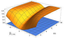
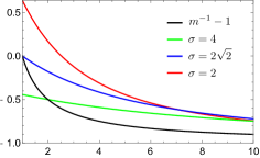
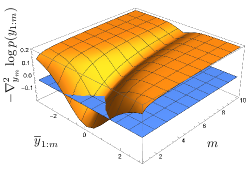
Figure 2: (a,b) The negative conditional Hessian for two values of σ𝜎\sigma are plotted as a function of y¯1:msubscript¯𝑦:1𝑚\overline{y}_{1:m} and m𝑚m assuming X𝑋X is distributed according to (4.4) in 1D, where we set μ=3𝜇3\mu=3, τ=1𝜏1\tau=1 (see (4.5)). (c) The upper bound in (4.1) is sharp for this example; σ2ζ(m)superscript𝜎2𝜁𝑚\sigma^{2}\zeta(m) is plotted vs. m𝑚m for different σ𝜎\sigma.

4.1 Example: Mixture of two Gaussians

In this section we examine Theorem 1 by studying the following mixture of Gaussians for α=1/2𝛼12\alpha=1/2:

p(x)=α𝒩(x;μ,τ2I)+(1α)𝒩(x;μ,τ2I).𝑝𝑥𝛼𝒩𝑥𝜇superscript𝜏2𝐼1𝛼𝒩𝑥𝜇superscript𝜏2𝐼p(x)=\alpha\,\mathcal{N}(x;\mu,\tau^{2}I)+(1-\alpha)\,\mathcal{N}(x;-\mu,\tau^{2}I). (4.4)

This is an instance of the setup in Theorem 1, where p(z)=12δ(zμ)+12δ(z+μ)𝑝𝑧12𝛿𝑧𝜇12𝛿𝑧𝜇p(z)=\frac{1}{2}\delta(z-\mu)+\frac{1}{2}\delta(z+\mu), and R2=μμsuperscript𝑅2superscript𝜇top𝜇R^{2}=\mu^{\top}\mu. By differentiating (2.2) twice we arrive at the following expression for ym2logp(ym|y1:m1)superscriptsubscriptsubscript𝑦𝑚2𝑝conditionalsubscript𝑦𝑚subscript𝑦:1𝑚1\nabla_{y_{m}}^{2}\log p(y_{m}|y_{1:m-1}):

ym2logp(ym|y1:m1)=ym2logp(y1:m)=σ2(m11)I+m2H(y¯1:m;m1/2σ),superscriptsubscriptsubscript𝑦𝑚2𝑝conditionalsubscript𝑦𝑚subscript𝑦:1𝑚1superscriptsubscriptsubscript𝑦𝑚2𝑝subscript𝑦:1𝑚superscript𝜎2superscript𝑚11𝐼superscript𝑚2𝐻subscript¯𝑦:1𝑚superscript𝑚12𝜎\nabla_{y_{m}}^{2}\log p(y_{m}|y_{1:m-1})=\nabla_{y_{m}}^{2}\log p(y_{1:m})=\sigma^{-2}(m^{-1}-1)I+m^{-2}H(\overline{y}_{1:m};m^{-1/2}\sigma), (4.5)

where

H(y;σ)2log𝔼X𝒩(y,σ2I)[ef(X)].𝐻𝑦𝜎superscript2subscript𝔼similar-to𝑋𝒩𝑦superscript𝜎2𝐼delimited-[]superscript𝑒𝑓𝑋H(y;\sigma)\coloneqq\nabla^{2}\log\mathbb{E}_{X\sim\mathcal{N}(y,\sigma^{2}I)}[e^{-f(X)}].

In Appendix D we show that for the mixture of Gaussian here, (4.4) with α=1/2𝛼12\alpha=1/2, we have

H(y;σ)=1(σ2+τ2)(I+2μμσ2+τ2(1+cosh(2μyσ2+τ2))1),𝐻𝑦𝜎1superscript𝜎2superscript𝜏2𝐼2𝜇superscript𝜇topsuperscript𝜎2superscript𝜏2superscript12superscript𝜇top𝑦superscript𝜎2superscript𝜏21H(y;\sigma)=\frac{1}{(\sigma^{2}+\tau^{2})}\biggl{(}-I+\frac{2\mu\mu^{\top}}{\sigma^{2}+\tau^{2}}\cdot\biggl{(}1+\cosh\Bigl{(}\frac{2\mu^{\top}y}{\sigma^{2}+\tau^{2}}\Bigr{)}\biggr{)}^{-1}\biggr{)}, (4.6)

which takes its maximum at y=0𝑦0y=0. By using (4.5), it is then straightforward to show that (4.1), (4.2), and (4.3) all hold in this example, with the additional result that the upper bound is now tight. In Fig. 2, these calculations are visualized in 1D for μ=3,τ=1formulae-sequence𝜇3𝜏1\mu=3,\tau=1, and for different values of σ𝜎\sigma; in panel (c) we also plot 11/m11𝑚1-1/m which is the large m𝑚m behavior of σ2ζ(m)superscript𝜎2𝜁𝑚\sigma^{2}\zeta(m). This can be seen from two different routes: (4.2) and (4.5).

Remark 3 (Monotonicity).

The monotonic decrease of the upper bound in Theorem 1, together with the monotonicity result in Lemma 2, may lead one to investigate whether the stronger result

y12logp(y1)y22logp(y2|y1)ym2logp(ym|y1:m1),succeeds-or-equalssuperscriptsubscriptsubscript𝑦12𝑝subscript𝑦1superscriptsubscriptsubscript𝑦22𝑝conditionalsubscript𝑦2subscript𝑦1succeeds-or-equalssucceeds-or-equalssuperscriptsubscriptsubscript𝑦𝑚2𝑝conditionalsubscript𝑦𝑚subscript𝑦:1𝑚1\nabla_{y_{1}}^{2}\log p(y_{1})\succcurlyeq\nabla_{y_{2}}^{2}\log p(y_{2}|y_{1})\succcurlyeq\dots\succcurlyeq\nabla_{y_{m}}^{2}\log p(y_{m}|y_{1:m-1}), (4.7)

could hold, e.g., for the mixture of Gaussians we studied here, especially since the upper bound (4.1) is sharp for this example. For (4.7) to hold, cov(Z|y1:m)covconditional𝑍subscript𝑦:1𝑚{{\rm cov}}(Z|y_{1:m}) must be less than cov(Z|y1:m1)covconditional𝑍subscript𝑦:1𝑚1{{\rm cov}}(Z|y_{1:m-1}). However, we can imagine a scenario where y1++ym1subscript𝑦1subscript𝑦𝑚1y_{1}+\dots+y_{m-1} is very large, so that cov(Z|y1:m)0covconditional𝑍subscript𝑦:1𝑚0{{\rm cov}}(Z|y_{1:m})\approx 0, while ymsubscript𝑦𝑚y_{m} is such that y1++ym1+ymsubscript𝑦1subscript𝑦𝑚1subscript𝑦𝑚y_{1}+\dots+y_{m-1}+y_{m} is close to m𝔼[Z]𝑚𝔼delimited-[]𝑍m\mathbb{E}[Z], where cov(Z|y1:m)covconditional𝑍subscript𝑦:1𝑚{{\rm cov}}(Z|y_{1:m}) will be large.

4.2 Algorithm: non-Markovian chain of (log-concave) Markov chains

Below, we give the pseudo-code for our sampling algorithm. In the inner loop, MCMCσsubscriptMCMC𝜎{\textrm{MCMC}}_{\sigma} is any MCMC method, but our focus in this paper is on Langevin MCMC algorithms222We experimented with a variety of Langevin MCMC algorithms to sample from p(yt|y1:t1)𝑝conditionalsubscript𝑦𝑡subscript𝑦:1𝑡1p(y_{t}|y_{1:t-1}) in the inner loop of Algorithm 1. The results are reported in the appendix due to space constraints. After extensive tuning, we found the underdamped Langevin MCMC algorithm by Sachs et al. (2017) to be the best performing for the test densities we considered. that use ytlogp(yt|y1:t1)subscriptsubscript𝑦𝑡𝑝conditionalsubscript𝑦𝑡subscript𝑦:1𝑡1\nabla_{y_{t}}\log p(y_{t}|y_{1:t-1}) to sample the new measurement Ytsubscript𝑌𝑡Y_{t} conditioned on the previously sampled ones Y1:t1subscript𝑌:1𝑡1Y_{1:t-1}.

1:  Parameter noise level σ𝜎\sigma
2:  Input number of measurements m𝑚m, number of steps for each measurement ntsubscript𝑛𝑡n_{t}
3:  Output X^^𝑋\hat{X}
14:  Initialize Y¯1:0=0subscript¯𝑌:100{\overline{Y}}_{1:0}=0
5:  for t=[1,,m]𝑡1𝑚t=[1,\dots,m] do
26:     Initialize Yt(0)superscriptsubscript𝑌𝑡0Y_{t}^{(0)}
3
7:     for i=[1,,nt]𝑖1subscript𝑛𝑡i=[1,\dots,n_{t}] do
48:        Yt(i)=MCMCσ(Yt(i1),Y¯1:t1)superscriptsubscript𝑌𝑡𝑖subscriptMCMC𝜎superscriptsubscript𝑌𝑡𝑖1subscript¯𝑌:1𝑡1Y_{t}^{(i)}={\textrm{MCMC}_{\sigma}}(Y_{t}^{(i-1)},{\overline{Y}_{1:t-1}})
59:     end for
10:     Yt=Yt(nt)subscript𝑌𝑡superscriptsubscript𝑌𝑡subscript𝑛𝑡Y_{t}=Y_{t}^{(n_{t})}
611:     Y¯1:t=Y¯1:t1+(YtY¯1:t1)/tsubscript¯𝑌:1𝑡subscript¯𝑌:1𝑡1subscript𝑌𝑡subscript¯𝑌:1𝑡1𝑡{\overline{Y}}_{1:t}={\overline{Y}}_{1:t-1}+(Y_{t}-{\overline{Y}}_{1:t-1})/t
12:  end for
13:  return  X^𝔼[X|Y1:m]^𝑋𝔼delimited-[]conditional𝑋subscript𝑌:1𝑚\hat{X}\leftarrow\mathbb{E}[X|Y_{1:m}] according to (2.3)
Algorithm 1 One-(measurement)-at-a-time walk-jump sampling referred to by OAT. See Fig. 1 for the schematic. A version of MCMCσsubscriptMCMC𝜎{\textrm{MCMC}}_{\sigma} is given in Appendix E.

4.2.1 Estimating logp(y)𝑝𝑦\nabla\log p(y)

So far we have assumed we know the smoothed score function g(y;σ)=(logp)(y)=φ(y;σ)𝑔𝑦𝜎𝑝𝑦𝜑𝑦𝜎g(y;\sigma)=\nabla(\log p)(y)=\nabla\varphi(y;\sigma), and in experiments below we consider cases where we know g(y;σ)𝑔𝑦𝜎g(y;\sigma) in closed form. But in principle, we would like to estimate g(y;σ)𝑔𝑦𝜎g(y;\sigma) in terms of the unnormalized p(x)ef(x)proportional-to𝑝𝑥superscript𝑒𝑓𝑥p(x)\propto e^{-f(x)}. The simplest such “plug-in” estimator is as follows (see Appendix B):

g^1(y;σ)=1σi=1nεiexp(f(y+σεi))i=1nexp(f(y+σεi)),εi𝒩(0,I).formulae-sequencesubscript^𝑔1𝑦𝜎1𝜎superscriptsubscript𝑖1𝑛subscript𝜀𝑖𝑓𝑦𝜎subscript𝜀𝑖superscriptsubscript𝑖1𝑛𝑓𝑦𝜎subscript𝜀𝑖similar-tosubscript𝜀𝑖𝒩0𝐼\hat{g}_{1}(y;\sigma)=\frac{1}{\sigma}\frac{\sum_{i=1}^{n}\varepsilon_{i}\exp\left(-f(y+\sigma\varepsilon_{i})\right)}{\sum_{i=1}^{n}\exp\left(-f(y+\sigma\varepsilon_{i})\right)},\;\varepsilon_{i}\sim\mathcal{N}(0,I). (4.8)

Using any estimator for (logp)(y)𝑝𝑦\nabla(\log p)(y), including g^1subscript^𝑔1\hat{g}_{1} above, we can construct an estimator for logp(ym|y1:m1)𝑝conditionalsubscript𝑦𝑚subscript𝑦:1𝑚1\nabla\log p(y_{m}|y_{1:m-1}) using results in Sec. 2, see (2.2), and Appendix A:

ymlogp(ym|y1:m1)=ymlogp(y1:m)1mg^(y¯1:m;σm)+1σ2(y¯1:myt).subscriptsubscript𝑦𝑚𝑝conditionalsubscript𝑦𝑚subscript𝑦:1𝑚1subscriptsubscript𝑦𝑚𝑝subscript𝑦:1𝑚1𝑚^𝑔subscript¯𝑦:1𝑚𝜎𝑚1superscript𝜎2subscript¯𝑦:1𝑚subscript𝑦𝑡\nabla_{y_{m}}\log p(y_{m}|y_{1:m-1})=\nabla_{y_{m}}\log p(y_{1:m})\approx\frac{1}{m}\hat{g}(\overline{y}_{1:m};\frac{\sigma}{\sqrt{m}})+\frac{1}{\sigma^{2}}(\overline{y}_{1:m}-y_{t}). (4.9)

In the appendix, we also conduct experiments to investigate this aspect of the problem. Studying the covariance of the plug-in estimator and devising better estimators is beyond the scope of this paper.

5 Experiments

We evaluate the performance of Algorithm 1 alongside related sampling schemes on carefully designed test densities. We compare the following sampling schemes:

  • One-at-a-time walk-jump sampling using Algorithm 1 with m=1000𝑚1000m=1000 (“OAT”),

  • All-at-once walk-jump sampling (“AAO”),

  • Single-measurement walk-jump sampling (“m=1𝑚1m=1”),

  • Langevin MCMC by Sachs et al. (2017) without any smoothing (“σ=0𝜎0\sigma=0”).

The hyperparameters were tuned for each sampling scheme and the total number of iterations was kept fixed. See Appendix F for details.
Refer to caption
Refer to caption
Refer to caption
Refer to caption
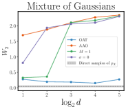
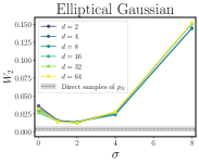
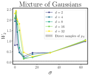
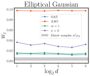
Figure 3: (a, b) 2-Wasserstein distance vs. d𝑑d and (c, d) 2-Wasserstein distance vs. σ𝜎\sigma for varying d𝑑d for the elliptical Gaussian and Gaussian mixture target densities.

Metric. We use the Wasserstein metric to quantify the consistency of the obtained samples with the target density pXsubscript𝑝𝑋p_{X}. In general, evaluation of Wasserstein distance between high-dimensional distributions is nontrivial, as it involves identifying an optimal coupling and solving a multivariate integral. We implement a simplified version of this metric by viewing our target measure as empirical and restricting our focus to a representative marginal dimension by projecting our samples X𝑋X from pXsubscript𝑝𝑋p_{X} and X^^𝑋\hat{X} from p^σ,msubscript^𝑝𝜎𝑚{\hat{p}}_{\sigma,m} to a chosen vector θ𝜃\theta in dsuperscript𝑑\mathbb{R}^{d}: X=θXsuperscript𝑋parallel-tosuperscript𝜃top𝑋X^{\parallel}=\theta^{\top}X\in\mathbb{R}. For one-dimensional empirical distributions, the 222-Wasserstein distance between pXsubscript𝑝𝑋p_{X} and p^σ,msubscript^𝑝𝜎𝑚{\hat{p}}_{\sigma,m} can be approximated as

W2(X,X^)21ni=1n|X(i)X^(i)|2,subscript𝑊2superscriptsuperscript𝑋parallel-tosuperscript^𝑋parallel-to21𝑛superscriptsubscript𝑖1𝑛superscriptsubscriptsuperscript𝑋parallel-to𝑖subscriptsuperscript^𝑋parallel-to𝑖2W_{2}(X^{\parallel},\hat{X}^{\parallel})^{2}\approx\frac{1}{n}\sum_{i=1}^{n}|X^{\parallel}_{(i)}-\hat{X}^{\parallel}_{(i)}|^{2},

where X(1),,X(n)subscriptsuperscript𝑋parallel-to1subscriptsuperscript𝑋parallel-to𝑛X^{\parallel}_{(1)},\cdots,X^{\parallel}_{(n)} are order statistics (Bonneel et al., 2015; Peyré & Cuturi, 2019).

MCMC algorithms. For all the results in this section, we implement MCMC sampling based on underdamped Langevin diffusion (ULD). The particular algorithm used for the results shown in this section extends the BAOAB integration scheme using multiple time steps for the O-part (Sachs et al., 2017). In Appendix G, we present the full comparison across other MCMC algorithms, including other recent ULD variants (Cheng et al., 2018; Shen & Lee, 2019) as well as the Metropolis-adjusted Langevin algorithm (MALA) (Roberts & Tweedie, 1996; Dwivedi et al., 2018).

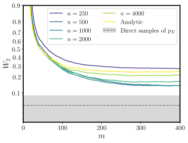
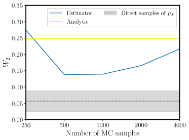
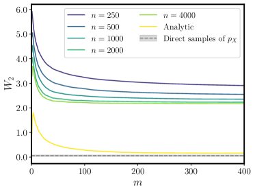
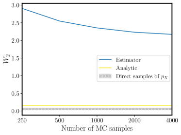
Score estimation. In Appendix H, we compare sampling with the analytic score function and the plug-in estimator of the score function given in (4.8) with varying numbers of MC samples n𝑛n.

5.1 Elliptical Gaussian

The elliptical Gaussian features a poorly conditioned covariance: pX(x)=𝒩(x; 0,C),subscript𝑝𝑋𝑥𝒩𝑥 0𝐶p_{X}(x)=\mathcal{N}\left(x;\ 0,C\right), where we set τ02=0.1,τ12==τd2=1formulae-sequencesuperscriptsubscript𝜏020.1superscriptsubscript𝜏12superscriptsubscript𝜏𝑑21\tau_{0}^{2}=0.1,\tau_{1}^{2}=\cdots=\tau_{d}^{2}=1 in (3.1). We evaluate the 2-Wasserstein distance on the “difficult” narrow dimension (with variance τ02superscriptsubscript𝜏02\tau_{0}^{2}). For each d𝑑d, the noise level σ𝜎\sigma and other hyperparameters of the sampling algorithm, such as step size and friction, were tuned. Fig. 3(a) plots the 2-Wasserstein distance with varying d𝑑d. OAT and m=1𝑚1m=1 outperform Langevin MCMC (σ=0𝜎0\sigma=0) for all d𝑑d, suggesting that smoothing offers an advantage. On the other hand, AAO struggles, which is expected from our theoretical analysis in Sec. 3. As Fig. 3(b) shows, OAT with σ=1𝜎1\sigma=1 and σ=2𝜎2\sigma=2 outperforms Langevin MCMC (σ=0𝜎0\sigma=0) for all d𝑑d. The optimal σ𝜎\sigma remains fairly constant with increasing d𝑑d.

5.2 Mixture of Gaussians

To evaluate mixing of multiple modes, we consider the mixture of Gaussians test density (4.4) with α=1/5𝛼15\alpha=\nicefrac{{1}}{{5}}, τ=1𝜏1\tau=1, and μ=31d𝜇3subscript1𝑑\mu=3\cdot 1_{d}, where 1dsubscript1𝑑1_{d} is the d𝑑d-dimensional vector (1,,1)superscript11top(1,\dots,1)^{\top}. As Fig. 3(a) shows, OAT achieves consistently low 2-Wasserstein distance with increasing d𝑑d, whereas other sampling schemes deteriorate in performance. We observe, in Fig. 3(b), that OAT outperforms the best-performing underdamped Langevin MCMC (σ=0𝜎0\sigma=0) in our experiments for at least one σ𝜎\sigma value for all d𝑑d. Higher d𝑑d requires larger σ𝜎\sigma. In addition, we would like to highlight the following: (I) Vanilla walk-jump sampling (m=1𝑚1m=1) is highly ineffective as the dimensions increase. This is in contrast to the sampling from anisotropic Gaussian (already log-concave) in Sec. 5.1. (II) The optimal σ𝜎\sigma here is in fact larger than the noise level needed to make p(y1)𝑝subscript𝑦1p(y_{1}) log-concave. This is related to the benefits of sampling from better-conditioned log-concave distributions, which is well-known in the literature. In Appendix I, we include results for a mixture of correlated Gaussians supporting the same conclusion.

5.3 Tunneling phenomena

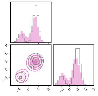
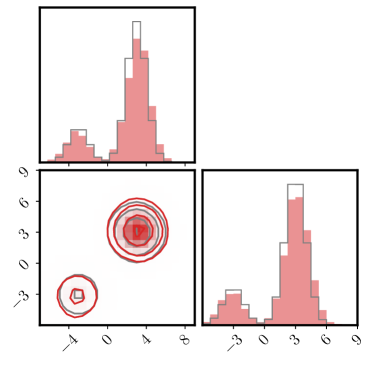
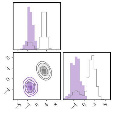
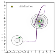
Fig. 4 illustrates the trajectories of three walkers (a) under our OAT sampling scheme and (b) using Langevin MCMC. Each walker has the same random seed between (a) and (b) and was initialized at (3,3)33(3,3), the dominant mode with 80% of the mass. With OAT, a walker is able to tunnel to the smaller mode fairly quickly, whereas for Langevin MCMC (without smoothing) all three walkers are stuck around the dominant mode. In panels (c) and (d) we also show the histogram of final samples in the same setup with initialization at (3,3)33(3,3) for 100 walkers after 100 K steps.

In summary of this section, we consistently observe that the same (Langevin) MCMC algorithm, when used in the inner loop of Algorithm 1, is more effective than when used without Gaussian smoothing.
Refer to caption
(a) OAT, 3 trajectories
Refer to caption
(b) Langevin MCMC
Refer to caption
(c) OAT, 100 samples
Refer to caption
(d) Langevin, 100 samples
Figure 4: Tunneling phenomenon. Trajectories of three walkers (a) under our OAT sampling scheme using Langevin MCMC by Sachs et al. (2017) in the inner loop of Algorithm 1 (b) the same Langevin MCMC without any smoothing. Purple and green indicate the beginning and end of trajectories, respectively. (c, d) The final samples for 100 random trajectories (using identical seeds).

6 Conclusion

In this paper, we established a theoretical framework that reduces the general problem of sampling from an unnormalized distribution to that of log-concave sampling defined by a single noise parameter. We conclude with two main limitations of this work at the present time: (I) Our results do not make it clear if the log-concave sampling strategy is optimal. The issue of “optimality” is challenging as it is inherently problem-dependent and additionally depends on the MCMC algorithm used in the inner loop of Algorithm 1. (II) Related to the issue of optimality is the fact that for general sampling problems, the smoothed score functions required to sample from p(yt|y1:t1)𝑝conditionalsubscript𝑦𝑡subscript𝑦:1𝑡1p(y_{t}|y_{1:t-1}), t[m]𝑡delimited-[]𝑚t\in[m] using gradient-based methods need to be estimated. This is a complex problem and should be investigated in future research. Finally, an immediate application of the machinery we developed here is the problem of generative modeling, as the m𝑚m smoothed score functions needed in running Algorithm 1 can indeed be learned (approximated) using empirical Bayes least-squares denoising objectives. This approach is similar to training diffusion models; however, our sampling scheme is fundamentally different, as it relies on the accumulation of measurements, controlled by a single noise parameter, σ𝜎\sigma.

References

  • Bonneel et al. (2015) Nicolas Bonneel, Julien Rabin, Gabriel Peyré, and Hanspeter Pfister. Sliced and radon Wasserstein barycenters of measures. Journal of Mathematical Imaging and Vision, 51:22–45, 2015.
  • Cao et al. (2020) Yu Cao, Jianfeng Lu, and Lihan Wang. Complexity of randomized algorithms for underdamped Langevin dynamics. arXiv preprint arXiv:2003.09906, 2020.
  • Cheng et al. (2018) Xiang Cheng, Niladri S. Chatterji, Peter L. Bartlett, and Michael I. Jordan. Underdamped Langevin MCMC: A non-asymptotic analysis. In Conference on Learning Theory, pp.  300–323, 2018.
  • Dalalyan (2017) Arnak S. Dalalyan. Theoretical guarantees for approximate sampling from smooth and log-concave densities. Journal of the Royal Statistical Society. Series B (Statistical Methodology), pp.  651–676, 2017.
  • Durmus & Moulines (2017) Alain Durmus and Éric Moulines. Nonasymptotic convergence analysis for the unadjusted Langevin algorithm. The Annals of Applied Probability, 27(3):1551 – 1587, 2017.
  • Dwivedi et al. (2018) Raaz Dwivedi, Yuansi Chen, Martin J. Wainwright, and Bin Yu. Log-concave sampling: Metropolis-Hastings algorithms are fast! In Conference on Learning Theory, pp.  793–797, 2018.
  • Ho et al. (2020) Jonathan Ho, Ajay Jain, and Pieter Abbeel. Denoising diffusion probabilistic models. Advances in Neural Information Processing Systems, 33:6840–6851, 2020.
  • Hyvärinen (2005) Aapo Hyvärinen. Estimation of non-normalized statistical models by score matching. Journal of Machine Learning Research, 6(Apr):695–709, 2005.
  • Karras et al. (2022) Tero Karras, Miika Aittala, Timo Aila, and Samuli Laine. Elucidating the design space of diffusion-based generative models. Advances in Neural Information Processing Systems, 35:26565–26577, 2022.
  • Kirkpatrick et al. (1983) Scott Kirkpatrick, C. Daniel Gelatt Jr., and Mario P. Vecchi. Optimization by simulated annealing. Science, 220(4598):671–680, 1983.
  • Leimkuhler & Matthews (2015) Ben Leimkuhler and Charles Matthews. Molecular dynamics: With deterministic and stochastic numerical methods. Interdisciplinary Applied Mathematics, 39:443, 2015.
  • Li et al. (2022) Ruilin Li, Hongyuan Zha, and Molei Tao. Sqrt(d) dimension dependence of Langevin Monte Carlo. In International Conference on Learning Representations, 2022.
  • Metropolis et al. (1953) Nicholas Metropolis, Arianna W. Rosenbluth, Marshall N. Rosenbluth, Augusta H. Teller, and Edward Teller. Equation of state calculations by fast computing machines. The Journal of Chemical Physics, 21(6):1087–1092, 1953.
  • Miyasawa (1961) Koichi Miyasawa. An empirical Bayes estimator of the mean of a normal population. Bulletin of the International Statistical Institute, 38(4):181–188, 1961.
  • Mou et al. (2021) Wenlong Mou, Yi-An Ma, Martin J. Wainwright, Peter L. Bartlett, and Michael I. Jordan. High-order Langevin diffusion yields an accelerated MCMC algorithm. Journal of Machine Learning Research, 22(1):1919–1959, 2021.
  • Neal (1995) Radford M. Neal. Bayesian learning for neural networks. 1995. PhD thesis, University of Toronto.
  • Neal (2001) Radford M. Neal. Annealed importance sampling. Statistics and Computing, 11:125–139, 2001.
  • Parisi (1981) Giorgio Parisi. Correlation functions and computer simulations. Nuclear Physics B, 180(3):378–384, 1981.
  • Peyré & Cuturi (2019) Gabriel Peyré and Marco Cuturi. Computational optimal transport: With applications to data science. Foundations and Trends® in Machine Learning, 11(5-6):355–607, 2019.
  • Robbins (1956) Herbert Robbins. An empirical Bayes approach to statistics. In Proc. Third Berkeley Symp., volume 1, pp.  157–163, 1956.
  • Roberts & Tweedie (1996) Gareth O. Roberts and Richard L. Tweedie. Exponential convergence of Langevin distributions and their discrete approximations. Bernoulli, pp.  341–363, 1996.
  • Sachs et al. (2017) Matthias Sachs, Benedict Leimkuhler, and Vincent Danos. Langevin dynamics with variable coefficients and nonconservative forces: from stationary states to numerical methods. Entropy, 19(12):647, 2017.
  • Saremi & Hyvärinen (2019) Saeed Saremi and Aapo Hyvärinen. Neural empirical Bayes. Journal of Machine Learning Research, 20(181):1–23, 2019.
  • Saremi & Srivastava (2022) Saeed Saremi and Rupesh Kumar Srivastava. Multimeasurement generative models. In International Conference on Learning Representations, 2022.
  • Shen & Lee (2019) Ruoqi Shen and Yin Tat Lee. The randomized midpoint method for log-concave sampling. Advances in Neural Information Processing Systems, 32, 2019.
  • Sohl-Dickstein et al. (2015) Jascha Sohl-Dickstein, Eric Weiss, Niru Maheswaranathan, and Surya Ganguli. Deep unsupervised learning using nonequilibrium thermodynamics. In International Conference on Machine Learning, pp. 2256–2265, 2015.
  • Syed et al. (2022) Saifuddin Syed, Alexandre Bouchard-Côté, George Deligiannidis, and Arnaud Doucet. Non-reversible parallel tempering: a scalable highly parallel MCMC scheme. Journal of the Royal Statistical Society Series B: Statistical Methodology, 84(2):321–350, 2022.
  • Villani (2021) Cédric Villani. Topics in Optimal Transportation, volume 58. American Mathematical Society, 2021.
  • Wainwright & Jordan (2008) Martin J. Wainwright and Michael I. Jordan. Graphical models, exponential families, and variational inference. Foundations and Trends in Machine Learning, 1(1–2):1–305, 2008.

Appendix A Derivations for Sec. 2

A.1 Derivation for (2.2)

In this section we derive a general expression for the (σ,m)𝜎𝑚(\sigma,m)-densities p(y1:m)𝑝subscript𝑦:1𝑚p(y_{1:m}), short for pσ(y1:m)subscript𝑝𝜎subscript𝑦:1𝑚p_{\sigma}(y_{1:m}):

p(y1:m)=dp(x)(t=1mp(yt|x))𝑑x=d1Zef(x)(t=1m1(2πσ2)d/2exp(12σ2xyt2))𝑑xdef(x)exp(12σ2t=1mxyt2)𝑑x.𝑝subscript𝑦:1𝑚subscriptsuperscript𝑑𝑝𝑥superscriptsubscriptproduct𝑡1𝑚𝑝conditionalsubscript𝑦𝑡𝑥differential-d𝑥subscriptsuperscript𝑑1𝑍superscript𝑒𝑓𝑥superscriptsubscriptproduct𝑡1𝑚1superscript2𝜋superscript𝜎2𝑑212superscript𝜎2superscriptdelimited-∥∥𝑥subscript𝑦𝑡2differential-d𝑥proportional-tosubscriptsuperscript𝑑superscript𝑒𝑓𝑥12superscript𝜎2superscriptsubscript𝑡1𝑚superscriptdelimited-∥∥𝑥subscript𝑦𝑡2differential-d𝑥\begin{split}p(y_{1:m})&=\int_{\mathbb{R}^{d}}p(x)\biggl{(}\prod_{t=1}^{m}p(y_{t}|x)\biggr{)}dx\\ &=\int_{\mathbb{R}^{d}}\frac{1}{Z}e^{-f(x)}\biggl{(}\prod_{t=1}^{m}\frac{1}{(2\pi\sigma^{2})^{d/2}}\exp\Bigl{(}-\frac{1}{2\sigma^{2}}{\big{\|}}x-y_{t}{\big{\|}}^{2}\Bigr{)}\biggr{)}dx\\ &\propto\int_{\mathbb{R}^{d}}e^{-f(x)}\exp\Bigl{(}-\frac{1}{2\sigma^{2}}\sum_{t=1}^{m}{\big{\|}}x-y_{t}{\big{\|}}^{2}\Bigr{)}dx.\end{split}

The (σ,m)𝜎𝑚(\sigma,m)-density is permutation invariant under the permutation π:[m][m]:𝜋delimited-[]𝑚delimited-[]𝑚\pi:[m]\rightarrow[m] of measurement indices. In the calculation below we derive a general form for (σ,m)𝜎𝑚(\sigma,m)-densities where this permutation invariance becomes apparent in terms of the empirical mean of the m𝑚m measurements

y¯1:m=1mt=1myt.subscript¯𝑦:1𝑚1𝑚superscriptsubscript𝑡1𝑚subscript𝑦𝑡\overline{y}_{1:m}=\frac{1}{m}\sum_{t=1}^{m}y_{t}.

and the empirical mean of {yt2}t=1msuperscriptsubscriptsuperscriptnormsubscript𝑦𝑡2𝑡1𝑚\{\|y_{t}\|^{2}\}_{t=1}^{m}. We start with a rewriting of logp(y1:m|x)𝑝conditionalsubscript𝑦:1𝑚𝑥\log p(y_{1:m}|x):

2σ2logp(y1:m|x)=m=1Mymx2+cst=mx22t=1myt,x+t=1myt2+cst=m(xy¯1:m2y¯1:m2+1mt=1myt2)+cst,2superscript𝜎2𝑝conditionalsubscript𝑦:1𝑚𝑥superscriptsubscript𝑚1𝑀superscriptdelimited-∥∥subscript𝑦𝑚𝑥2cst𝑚superscriptdelimited-∥∥𝑥22superscriptsubscript𝑡1𝑚subscript𝑦𝑡𝑥superscriptsubscript𝑡1𝑚superscriptdelimited-∥∥subscript𝑦𝑡2cst𝑚superscriptdelimited-∥∥𝑥subscript¯𝑦:1𝑚2superscriptdelimited-∥∥subscript¯𝑦:1𝑚21𝑚superscriptsubscript𝑡1𝑚superscriptdelimited-∥∥subscript𝑦𝑡2cst\begin{split}-2\sigma^{2}\log p(y_{1:m}|x)&=\sum_{m=1}^{M}{\big{\|}}y_{m}-x\|^{2}+{{\rm cst}}\\ &=m\|x\|^{2}-2\langle\sum_{t=1}^{m}y_{t},x\rangle+\sum_{t=1}^{m}\|y_{t}\|^{2}+{{\rm cst}}\\ &=m\Bigl{(}\|x-\overline{y}_{1:m}\|^{2}-\|\overline{y}_{1:m}\|^{2}+\frac{1}{m}\sum_{t=1}^{m}\|y_{t}\|^{2}\Bigr{)}+{{\rm cst}},\end{split}

where cstcst{{\rm cst}} is a constant that does not depend on y1:msubscript𝑦:1𝑚y_{1:m}. Now, we view the smoothing kernel p(y1:m|x)𝑝conditionalsubscript𝑦:1𝑚𝑥p(y_{1:m}|x) as a Gaussian distribution centered at y¯¯𝑦\overline{y}:

logp(y1:m)=logef(x)p(y1:m|x)𝑑x+cst=logef(x)𝒩(x;y¯,m1σ2Id)𝑑x+y¯1:m2m1t=1myt22m1σ2+cst=log𝔼x𝒩(y¯1:m,m1σ2I)[ef(x)]+y¯1:m2m1t=1myt22m1σ2+cst.𝑝subscript𝑦:1𝑚superscript𝑒𝑓𝑥𝑝conditionalsubscript𝑦:1𝑚𝑥differential-d𝑥cstsuperscript𝑒𝑓𝑥𝒩𝑥¯𝑦superscript𝑚1superscript𝜎2subscript𝐼𝑑differential-d𝑥superscriptnormsubscript¯𝑦:1𝑚2superscript𝑚1superscriptsubscript𝑡1𝑚superscriptnormsubscript𝑦𝑡22superscript𝑚1superscript𝜎2cstsubscript𝔼similar-to𝑥𝒩subscript¯𝑦:1𝑚superscript𝑚1superscript𝜎2𝐼delimited-[]superscript𝑒𝑓𝑥superscriptnormsubscript¯𝑦:1𝑚2superscript𝑚1superscriptsubscript𝑡1𝑚superscriptnormsubscript𝑦𝑡22superscript𝑚1superscript𝜎2cst\begin{split}&\log p(y_{1:m})=\log\int e^{-f(x)}p(y_{1:m}|x)\,dx+{{\rm cst}}\\ &=\log\int e^{-f(x)}\mathcal{N}(x;\overline{y},m^{-1}\sigma^{2}I_{d})\,dx+\frac{\|\overline{y}_{1:m}\|^{2}-m^{-1}\sum_{t=1}^{m}\|y_{t}\|^{2}}{2m^{-1}\sigma^{2}}+{{\rm cst}}\\ &=\log\mathbb{E}_{x\sim\mathcal{N}(\overline{y}_{1:m},m^{-1}\sigma^{2}I)}[e^{-f(x)}]+\frac{\|\overline{y}_{1:m}\|^{2}-m^{-1}\sum_{t=1}^{m}\|y_{t}\|^{2}}{2m^{-1}\sigma^{2}}+{{\rm cst}}.\end{split}

The equation above reduces to (2.2) with the following definition

φ(y;σ)log𝔼x𝒩(y,σ2I)[ef(x)].𝜑𝑦𝜎subscript𝔼similar-to𝑥𝒩𝑦superscript𝜎2𝐼delimited-[]superscript𝑒𝑓𝑥\varphi(y;\sigma)\coloneqq\log\mathbb{E}_{x\sim\mathcal{N}(y,\sigma^{2}I)}[e^{-f(x)}].

A.2 Derivation for (2.3)

Next, we derive the expression for x^(y1:m)=𝔼[X|y1:m]^𝑥subscript𝑦:1𝑚𝔼delimited-[]conditional𝑋subscript𝑦:1𝑚\hat{x}(y_{1:m})=\mathbb{E}[X|y_{1:m}] given in (2.3):

𝔼[X|y1:m]=yt+σ2ytlogp(y1:m)=yt+σ2(m1φ(y¯1:m;m1/2σ)+σ2(y¯1:myt))=y¯1:m+m1σ2φ(y¯1:m;m1/2σ).𝔼delimited-[]conditional𝑋subscript𝑦:1𝑚subscript𝑦𝑡superscript𝜎2subscriptsubscript𝑦𝑡𝑝subscript𝑦:1𝑚subscript𝑦𝑡superscript𝜎2superscript𝑚1𝜑subscript¯𝑦:1𝑚superscript𝑚12𝜎superscript𝜎2subscript¯𝑦:1𝑚subscript𝑦𝑡subscript¯𝑦:1𝑚superscript𝑚1superscript𝜎2𝜑subscript¯𝑦:1𝑚superscript𝑚12𝜎\begin{split}\mathbb{E}[X|y_{1:m}]&=y_{t}+\sigma^{2}\nabla_{y_{t}}\log p(y_{1:m})\\ &=y_{t}+\sigma^{2}\bigl{(}m^{-1}\nabla\varphi(\overline{y}_{1:m};m^{-1/2}\sigma)+\sigma^{-2}(\overline{y}_{1:m}-y_{t})\bigr{)}\\ &=\overline{y}_{1:m}+m^{-1}\sigma^{2}\nabla\varphi(\overline{y}_{1:m};m^{-1/2}\sigma).\end{split} (A.1)

The first equation above comes from the generalization of the Bayes estimator to factorial kernels (Saremi & Srivastava, 2022), and for the second equation we used (2.2).

Appendix B Smoothed score functions

In this section, we give several different expressions related to smoothed densities used in the paper. We consider Y𝒩(X,σ2I)similar-to𝑌𝒩𝑋superscript𝜎2𝐼Y\sim\mathcal{N}(X,\sigma^{2}I) where Xef(x)similar-to𝑋superscript𝑒𝑓𝑥X\sim e^{-f(x)} in dsuperscript𝑑\mathbb{R}^{d}, thus with the density

p(y)=1Zef(x)1(2πσ2)d/2e12σ2xy2𝑑xef(x)e12σ2xy2𝑑x.𝑝𝑦1𝑍superscript𝑒𝑓𝑥1superscript2𝜋superscript𝜎2𝑑2superscript𝑒12superscript𝜎2superscriptnorm𝑥𝑦2differential-d𝑥proportional-tosuperscript𝑒𝑓𝑥superscript𝑒12superscript𝜎2superscriptnorm𝑥𝑦2differential-d𝑥p(y)=\int\frac{1}{Z}e^{-f(x)}\frac{1}{(2\pi\sigma^{2})^{d/2}}e^{-\frac{1}{2\sigma^{2}}\|x-y\|^{2}}dx\propto\int e^{-f(x)}e^{-\frac{1}{2\sigma^{2}}\|x-y\|^{2}}dx.

We have the following expressions for logp(y)𝑝𝑦\log p(y):

logp(y)𝑝𝑦\displaystyle\log p(y) =logef(x)e12σ2xy2𝑑x+cst,absentsuperscript𝑒𝑓𝑥superscript𝑒12superscript𝜎2superscriptnorm𝑥𝑦2differential-d𝑥cst\displaystyle=\log\int e^{-f(x)}e^{-\frac{1}{2\sigma^{2}}\|x-y\|^{2}}dx+{{\rm cst}},
logp(y)𝑝𝑦\displaystyle\log p(y) =logef(x+y)e12σ2x2𝑑x+cst,absentsuperscript𝑒𝑓𝑥𝑦superscript𝑒12superscript𝜎2superscriptnorm𝑥2differential-d𝑥cst\displaystyle=\log\int e^{-f(x+y)}e^{-\frac{1}{2\sigma^{2}}\|x\|^{2}}dx+{{\rm cst}},

leading to

(logp)(y)𝑝𝑦\displaystyle\nabla(\log p)(y) =ef(x)e12σ2xy2xyσ2𝑑xef(x)e12σ2xy2𝑑x=1σ2(𝔼[X|y]y),absentsuperscript𝑒𝑓𝑥superscript𝑒12superscript𝜎2superscriptnorm𝑥𝑦2𝑥𝑦superscript𝜎2differential-d𝑥superscript𝑒𝑓𝑥superscript𝑒12superscript𝜎2superscriptnorm𝑥𝑦2differential-d𝑥1superscript𝜎2𝔼delimited-[]conditional𝑋𝑦𝑦\displaystyle=\frac{\int e^{-f(x)}e^{-\frac{1}{2\sigma^{2}}\|x-y\|^{2}}\frac{x-y}{\sigma^{2}}dx}{\int e^{-f(x)}e^{-\frac{1}{2\sigma^{2}}\|x-y\|^{2}}dx}=\frac{1}{\sigma^{2}}(\mathbb{E}[X|y]-y),
(logp)(y)𝑝𝑦\displaystyle\nabla(\log p)(y) =ef(x+y)f(x+y)e12σ2x2𝑑xef(x+y)e12σ2x2𝑑xabsentsuperscript𝑒𝑓𝑥𝑦𝑓𝑥𝑦superscript𝑒12superscript𝜎2superscriptnorm𝑥2differential-d𝑥superscript𝑒𝑓𝑥𝑦superscript𝑒12superscript𝜎2superscriptnorm𝑥2differential-d𝑥\displaystyle=-\frac{\int e^{-f(x+y)}\nabla f(x+y)e^{-\frac{1}{2\sigma^{2}}\|x\|^{2}}dx}{\int e^{-f(x+y)}e^{-\frac{1}{2\sigma^{2}}\|x\|^{2}}dx}
=ef(x)f(x)e12σ2xy2𝑑xef(x)e12σ2xy2𝑑x=𝔼[f(X)|y].absentsuperscript𝑒𝑓𝑥𝑓𝑥superscript𝑒12superscript𝜎2superscriptnorm𝑥𝑦2differential-d𝑥superscript𝑒𝑓𝑥superscript𝑒12superscript𝜎2superscriptnorm𝑥𝑦2differential-d𝑥𝔼delimited-[]conditional𝑓𝑋𝑦\displaystyle=-\frac{\int e^{-f(x)}\nabla f(x)e^{-\frac{1}{2\sigma^{2}}\|x-y\|^{2}}dx}{\int e^{-f(x)}e^{-\frac{1}{2\sigma^{2}}\|x-y\|^{2}}dx}=-\mathbb{E}[\nabla f(X)|y].

This in turn leads to three expressions for the Hessian:

2(logp)(y)superscript2𝑝𝑦\displaystyle\nabla^{2}(\log p)(y) =1σ2I+1σ4(𝔼[x(xy)|y]𝔼[x|y]𝔼[xy|y])absent1superscript𝜎2𝐼1superscript𝜎4𝔼delimited-[]conditional𝑥superscript𝑥𝑦top𝑦𝔼delimited-[]conditional𝑥𝑦𝔼superscriptdelimited-[]𝑥conditional𝑦𝑦top\displaystyle=-\frac{1}{\sigma^{2}}I+\frac{1}{\sigma^{4}}\left(\mathbb{E}\left[x(x-y)^{\top}|y\right]-\mathbb{E}\left[x|y\right]\mathbb{E}\left[x-y|y\right]^{\top}\right)
=1σ2I+1σ4(𝔼[xx|y]𝔼[x|y]𝔼[x|y])=1σ2I+1σ4cov(X|y),absent1superscript𝜎2𝐼1superscript𝜎4𝔼delimited-[]conditional𝑥superscript𝑥top𝑦𝔼delimited-[]conditional𝑥𝑦𝔼superscriptdelimited-[]conditional𝑥𝑦top1superscript𝜎2𝐼1superscript𝜎4covconditional𝑋𝑦\displaystyle=-\frac{1}{\sigma^{2}}I+\frac{1}{\sigma^{4}}\left(\mathbb{E}\left[xx^{\top}|y\right]-\mathbb{E}\left[x|y\right]\mathbb{E}\left[x|y\right]^{\top}\right)=-\frac{1}{\sigma^{2}}I+\frac{1}{\sigma^{4}}{{\rm cov}}(X|y), (B.1)
2(logp)(y)superscript2𝑝𝑦\displaystyle\nabla^{2}(\log p)(y) =𝔼[2f(X)|y]+𝔼[f(X)f(X)|y]+𝔼[f(X)|y]𝔼[f(X)|y]absent𝔼delimited-[]conditionalsuperscript2𝑓𝑋𝑦𝔼delimited-[]conditional𝑓𝑋𝑓superscript𝑋top𝑦𝔼delimited-[]conditional𝑓𝑋𝑦𝔼superscriptdelimited-[]conditional𝑓𝑋𝑦top\displaystyle=-\mathbb{E}[\nabla^{2}f(X)|y]+\mathbb{E}[\nabla f(X)\nabla f(X)^{\top}|y]+\mathbb{E}[\nabla f(X)|y]\mathbb{E}[\nabla f(X)|y]^{\top}
=𝔼[2f(X)|y]+cov(f(X)|y),absent𝔼delimited-[]conditionalsuperscript2𝑓𝑋𝑦covconditional𝑓𝑋𝑦\displaystyle=-\mathbb{E}[\nabla^{2}f(X)|y]+{{\rm cov}}(\nabla f(X)|y), (B.2)
2(logp)(y)superscript2𝑝𝑦\displaystyle\nabla^{2}(\log p)(y) =1σ2(𝔼[(xy)f(x)|y]𝔼[(xy)|y]𝔼[f(x)|y])absent1superscript𝜎2𝔼delimited-[]conditional𝑥𝑦𝑓superscript𝑥top𝑦𝔼delimited-[]conditional𝑥𝑦𝑦𝔼superscriptdelimited-[]conditional𝑓𝑥𝑦top\displaystyle=-\frac{1}{\sigma^{2}}\left(\mathbb{E}\left[(x-y)\nabla f(x)^{\top}|y\right]-\mathbb{E}\left[(x-y)|y\right]\mathbb{E}\left[\nabla f(x)|y\right]^{\top}\right)
=1σ2(𝔼[xf(x)|y]𝔼[x|y]𝔼[f(x)|y])=1σ2cov(X,f(X)|y).absent1superscript𝜎2𝔼delimited-[]conditional𝑥𝑓superscript𝑥top𝑦𝔼delimited-[]conditional𝑥𝑦𝔼superscriptdelimited-[]conditional𝑓𝑥𝑦top1superscript𝜎2cov𝑋conditional𝑓𝑋𝑦\displaystyle=-\frac{1}{\sigma^{2}}\left(\mathbb{E}\left[x\nabla f(x)^{\top}|y\right]-\mathbb{E}\left[x|y\right]\mathbb{E}\left[\nabla f(x)|y\right]^{\top}\right)=-\frac{1}{\sigma^{2}}{{\rm cov}}(X,\nabla f(X)|y).

B.1 Gaussian example

If X𝒩(μ,C)similar-to𝑋𝒩𝜇𝐶X\sim\mathcal{N}(\mu,C), then Y𝒩(μ,C+σ2I)similar-to𝑌𝒩𝜇𝐶superscript𝜎2𝐼Y\sim\mathcal{N}(\mu,C+\sigma^{2}I), and then

𝔼[X|Y]𝔼delimited-[]conditional𝑋𝑌\displaystyle\mathbb{E}[X|Y] =μ+C(C+σ2I)1(Yμ),absent𝜇𝐶superscript𝐶superscript𝜎2𝐼1𝑌𝜇\displaystyle=\mu+C(C+\sigma^{2}I)^{-1}(Y-\mu),
cov(X|Y)covconditional𝑋𝑌\displaystyle{{\rm cov}}(X|Y) =CC(C+σ2I)1C.absent𝐶𝐶superscript𝐶superscript𝜎2𝐼1𝐶\displaystyle=C-C(C+\sigma^{2}I)^{-1}C.

Therefore, 𝔼[X|Y]𝔼delimited-[]conditional𝑋𝑌\mathbb{E}[X|Y] is Gaussian with mean μ𝜇\mu and the covariance matrix C(C+σ2I)1C𝐶superscript𝐶superscript𝜎2𝐼1𝐶C(C+\sigma^{2}I)^{-1}C. We have 2(logp)(y)=(C+σ2I)1.superscript2𝑝𝑦superscript𝐶superscript𝜎2𝐼1-\nabla^{2}(\log p)(y)=(C+\sigma^{2}I)^{-1}.

B.2 Distribution of 𝔼[X|Y]𝔼delimited-[]conditional𝑋𝑌\mathbb{E}[X|Y]

If Y𝑌Y is sampled from pYsubscript𝑝𝑌p_{Y}, let p^σsubscript^𝑝𝜎\hat{p}_{\sigma} be the distribution of 𝔼[X|Y]=Y+σ2(logp)(Y)𝔼delimited-[]conditional𝑋𝑌𝑌superscript𝜎2𝑝𝑌\mathbb{E}[X|Y]=Y+\sigma^{2}\nabla(\log p)(Y). We can bound the 2-Wasserstein distance between p𝑝p and p^σsubscript^𝑝𝜎\hat{p}_{\sigma}, by sampling X𝑋X from pXsubscript𝑝𝑋p_{X}, and taking x^=Y+σ2logp(Y)^𝑥𝑌superscript𝜎2𝑝𝑌\hat{x}=Y+\sigma^{2}\nabla\log p(Y), where Y𝒩(X,σ2I)similar-to𝑌𝒩𝑋superscript𝜎2𝐼Y\sim\mathcal{N}(X,\sigma^{2}I). This leads to a particular “coupling” (Villani, 2021) between p𝑝p and p^σsubscript^𝑝𝜎\hat{p}_{\sigma}. It follows:

W2(p,p^σ)2𝔼X,Y𝔼[X|Y]X2.W_{2}(p,\hat{p}_{\sigma})^{2}\leqslant\mathbb{E}_{X,Y}\|\mathbb{E}[X|Y]-X\|^{2}.

Given that the conditional expectation 𝔼[X|Y]𝔼delimited-[]conditional𝑋𝑌\mathbb{E}[X|Y] is the optimal estimator for the square loss, the last expression is less than the trival estimator Y𝑌Y, that is,

W2(p,p^σ)2𝔼X,YYX2=σ2d.subscript𝑊2superscript𝑝subscript^𝑝𝜎2subscript𝔼𝑋𝑌superscriptnorm𝑌𝑋2superscript𝜎2𝑑W_{2}(p,\hat{p}_{\sigma})^{2}\leqslant\mathbb{E}_{X,Y}\|Y-X\|^{2}=\sigma^{2}d. (B.3)

B.3 Proposition 2

The calculations in Sec. B.2 that resulted in (B.3) leads to the following:

Proof for Proposition 2.

Using Proposition 1, we have

W2(p,p^σ,m)=W2(p,p^m1/2σ),subscript𝑊2𝑝subscript^𝑝𝜎𝑚subscript𝑊2𝑝subscript^𝑝superscript𝑚12𝜎W_{2}(p,\hat{p}_{\sigma,m})=W_{2}(p,\hat{p}_{m^{-1/2}\sigma}),

which is then combined with (B.3):

W2(p,p^σ,m)2σ2md.subscript𝑊2superscript𝑝subscript^𝑝𝜎𝑚2superscript𝜎2𝑚𝑑W_{2}(p,\hat{p}_{\sigma,m})^{2}\leqslant\frac{\sigma^{2}}{m}d.

Appendix C Proofs for Sec. 3

C.1 Proposition 3

Proof for Proposition 3.

We start with an expression for logp(y1:m)𝑝subscript𝑦:1𝑚\log p(y_{1:m}):

logp(y1:m)=logd(k=1m𝒩(x;yk,σ2I))𝒩(x;0,C)𝑑x=i=1dlogexp(k=1m(ykixi)22σ2xi22τi2)𝑑xi+cst=i=1dlogexp((xiαi)22βi2γi)𝑑xi+cst.𝑝subscript𝑦:1𝑚subscriptsuperscript𝑑superscriptsubscriptproduct𝑘1𝑚𝒩𝑥subscript𝑦𝑘superscript𝜎2𝐼𝒩𝑥0𝐶differential-d𝑥superscriptsubscript𝑖1𝑑subscriptsuperscriptsubscript𝑘1𝑚superscriptsubscript𝑦𝑘𝑖subscript𝑥𝑖22superscript𝜎2superscriptsubscript𝑥𝑖22superscriptsubscript𝜏𝑖2differential-dsubscript𝑥𝑖cstsuperscriptsubscript𝑖1𝑑subscriptsuperscriptsubscript𝑥𝑖subscript𝛼𝑖22superscriptsubscript𝛽𝑖2subscript𝛾𝑖differential-dsubscript𝑥𝑖cst\begin{split}\log p(y_{1:m})&=\log\int_{\mathbb{R}^{d}}\left(\prod_{k=1}^{m}\mathcal{N}(x;y_{k},\sigma^{2}I)\right)\mathcal{N}(x;0,C)\;dx\\ &=\sum_{i=1}^{d}\log\int_{\mathbb{R}}\exp{\left(-\sum_{k=1}^{m}\frac{\left(y_{ki}-x_{i}\right)^{2}}{2\sigma^{2}}-\frac{x_{i}^{2}}{2\tau_{i}^{2}}\right)}dx_{i}+{{\rm cst}}\\ &=\sum_{i=1}^{d}\log\int_{\mathbb{R}}\exp{\left(-\frac{(x_{i}-\alpha_{i})^{2}}{2\beta_{i}^{2}}-\gamma_{i}\right)}dx_{i}+{{\rm cst}}.\end{split} (C.1)

The expressions for αisubscript𝛼𝑖\alpha_{i}, βisubscript𝛽𝑖\beta_{i}, and γisubscript𝛾𝑖\gamma_{i} are given next by completing the square via matching second, first and zeroth derivative (in that order) of the left and right hand sides below

t=1m(ytixi)22σ2xi22τi2=(xiαi)22βi2γisuperscriptsubscript𝑡1𝑚superscriptsubscript𝑦𝑡𝑖subscript𝑥𝑖22superscript𝜎2superscriptsubscript𝑥𝑖22superscriptsubscript𝜏𝑖2superscriptsubscript𝑥𝑖subscript𝛼𝑖22superscriptsubscript𝛽𝑖2subscript𝛾𝑖-\sum_{t=1}^{m}\frac{\left(y_{ti}-x_{i}\right)^{2}}{2\sigma^{2}}-\frac{x_{i}^{2}}{2\tau_{i}^{2}}=-\frac{(x_{i}-\alpha_{i})^{2}}{2\beta_{i}^{2}}-\gamma_{i}

evaluated at xi=0subscript𝑥𝑖0x_{i}=0. The following three equations follow:

1βi21superscriptsubscript𝛽𝑖2\displaystyle\frac{1}{\beta_{i}^{2}} =mσ2+1τi2,absent𝑚superscript𝜎21superscriptsubscript𝜏𝑖2\displaystyle=\frac{m}{\sigma^{2}}+\frac{1}{\tau_{i}^{2}},
αiβi2=t=1mytiσ2αisubscript𝛼𝑖superscriptsubscript𝛽𝑖2superscriptsubscript𝑡1𝑚subscript𝑦𝑡𝑖superscript𝜎2subscript𝛼𝑖\displaystyle\frac{\alpha_{i}}{\beta_{i}^{2}}=\sum_{t=1}^{m}\frac{y_{ti}}{\sigma^{2}}\Rightarrow\alpha_{i} =1m+σ2τi2t=1myti,absent1𝑚superscript𝜎2superscriptsubscript𝜏𝑖2superscriptsubscript𝑡1𝑚subscript𝑦𝑡𝑖\displaystyle=\frac{1}{m+\sigma^{2}\tau_{i}^{-2}}\sum_{t=1}^{m}y_{ti},
αi22βi2γi=t=1myti22σ2γisuperscriptsubscript𝛼𝑖22superscriptsubscript𝛽𝑖2subscript𝛾𝑖superscriptsubscript𝑡1𝑚superscriptsubscript𝑦𝑡𝑖22superscript𝜎2subscript𝛾𝑖\displaystyle-\frac{\alpha_{i}^{2}}{2\beta_{i}^{2}}-\gamma_{i}=-\sum_{t=1}^{m}\frac{y_{ti}^{2}}{2\sigma^{2}}\Rightarrow\gamma_{i} =t=1myti22σ212σ2(m+σ2τi2)(t=1myti)2.absentsuperscriptsubscript𝑡1𝑚superscriptsubscript𝑦𝑡𝑖22superscript𝜎212superscript𝜎2𝑚superscript𝜎2superscriptsubscript𝜏𝑖2superscriptsuperscriptsubscript𝑡1𝑚subscript𝑦𝑡𝑖2\displaystyle=\sum_{t=1}^{m}\frac{y_{ti}^{2}}{2\sigma^{2}}-\frac{1}{2\sigma^{2}(m+\sigma^{2}\tau_{i}^{-2})}\Bigl{(}\sum_{t=1}^{m}y_{ti}\Bigr{)}^{2}.

It is convenient to define:

Ati=1t+σ2τi2.subscript𝐴𝑡𝑖1𝑡superscript𝜎2superscriptsubscript𝜏𝑖2A_{ti}=\frac{1}{t+\sigma^{2}\tau_{i}^{-2}}. (C.2)

Using above expressions, (C.1) simplifies to:

logp(y1:m)=i=1dγi+cst=t=1myt22σ2+12σ2i=1dAmi(t=1myti)2+cst.𝑝subscript𝑦:1𝑚superscriptsubscript𝑖1𝑑subscript𝛾𝑖cstsuperscriptsubscript𝑡1𝑚superscriptnormsubscript𝑦𝑡22superscript𝜎212superscript𝜎2superscriptsubscript𝑖1𝑑subscript𝐴𝑚𝑖superscriptsuperscriptsubscript𝑡1𝑚subscript𝑦𝑡𝑖2cst\log p(y_{1:m})=-\sum_{i=1}^{d}\gamma_{i}+{{\rm cst}}\\ =-\sum_{t=1}^{m}\frac{\|y_{t}\|^{2}}{2\sigma^{2}}+\frac{1}{2\sigma^{2}}\sum_{i=1}^{d}A_{mi}\Bigl{(}\sum_{t=1}^{m}y_{ti}\Bigr{)}^{2}+{{\rm cst}}. (C.3)

The energy function can be written more compactly by introducing the matrix Fσ,msubscript𝐹𝜎𝑚F_{\sigma,m}:

logp(y1:m)=12y1:mFσ,my1:m,σ2[Fσ,m]ti,ti=((1Ami)δttAmi(1δtt))δii.formulae-sequence𝑝subscript𝑦:1𝑚12superscriptsubscript𝑦:1𝑚topsubscript𝐹𝜎𝑚subscript𝑦:1𝑚superscript𝜎2subscriptdelimited-[]subscript𝐹𝜎𝑚𝑡𝑖superscript𝑡superscript𝑖1subscript𝐴𝑚𝑖subscript𝛿𝑡superscript𝑡subscript𝐴𝑚𝑖1subscript𝛿𝑡superscript𝑡subscript𝛿𝑖superscript𝑖\begin{split}\log p(y_{1:m})&=-\frac{1}{2}y_{1:m}^{\top}F_{\sigma,m}y_{1:m},\\ \sigma^{2}[F_{\sigma,m}]_{ti,t^{\prime}i^{\prime}}&=\left((1-A_{mi})\delta_{tt^{\prime}}-A_{mi}(1-\delta_{tt^{\prime}})\right)\delta_{ii^{\prime}}.\end{split}

In words, the md×md𝑚𝑑𝑚𝑑md\times md dimensional matrix Fσ,msubscript𝐹𝜎𝑚F_{\sigma,m} is block diagonal with d𝑑d blocks of size m×m𝑚𝑚m\times m. The blocks themselves capture the interactions between different measurements indexed by t𝑡t and tsuperscript𝑡t^{\prime}: The m×m𝑚𝑚m\times m blocks of the matrix Fσ,msubscript𝐹𝜎𝑚F_{\sigma,m}, indexed by i[d]𝑖delimited-[]𝑑i\in[d] thus have the form:

σ2Fσ,m(i)=(1Ami)Im+Ami(Im1m1m),superscript𝜎2superscriptsubscript𝐹𝜎𝑚𝑖1subscript𝐴𝑚𝑖subscript𝐼𝑚subscript𝐴𝑚𝑖subscript𝐼𝑚subscript1𝑚superscriptsubscript1𝑚top\sigma^{2}F_{\sigma,m}^{(i)}=(1-A_{mi})I_{m}+A_{mi}(I_{m}-1_{m}1_{m}^{\top}),

where 1m=(1,1,,1)superscriptsubscript1𝑚top1111_{m}^{\top}=(1,1,\dots,1) is m𝑚m-dimensional. It is straightforward to find the m𝑚m eigenvalues of the m×m𝑚𝑚m\times m matrix Fσ,m(i)superscriptsubscript𝐹𝜎𝑚𝑖F_{\sigma,m}^{(i)} for i[d]𝑖delimited-[]𝑑i\in[d]:

  • m1𝑚1m-1 degenerate eigenvalues equal to σ2superscript𝜎2\sigma^{-2} corresponding to the eigenvectors

    {(1,1,0,,0),(1,0,1,,0),,(1,0,0,,1)},superscript1100topsuperscript1010topsuperscript1001top\{(1,-1,0,\dots,0)^{\top},(1,0,-1,\dots,0)^{\top},\dots,(1,0,0,\dots,-1)^{\top}\},
  • one eigenvalue equal to σ2(1mAmi)superscript𝜎21𝑚subscript𝐴𝑚𝑖\sigma^{-2}(1-mA_{mi}) corresponding to the eigenvector (1,1,,1)superscript111top(1,1,\dots,1)^{\top}.

Since mAmi>0𝑚subscript𝐴𝑚𝑖0mA_{mi}>0 we have:

λmax(Fσ,m)=σ2,subscript𝜆maxsubscript𝐹𝜎𝑚superscript𝜎2\lambda_{\rm max}(F_{\sigma,m})=\sigma^{-2},

which is (m1)d𝑚1𝑑(m-1)d degenerate. The remaining d𝑑d eigenvalues are {σ2(1mAmi)}i[d]subscriptsuperscript𝜎21𝑚subscript𝐴𝑚𝑖𝑖delimited-[]𝑑\{\sigma^{-2}(1-mA_{mi})\}_{i\in[d]}, the smallest of which is given by

λmin(Fσ,m)=σ2(1mm+σ2τmax2)=σ21+mσ2τmax2.subscript𝜆minsubscript𝐹𝜎𝑚superscript𝜎21𝑚𝑚superscript𝜎2superscriptsubscript𝜏max2superscript𝜎21𝑚superscript𝜎2superscriptsubscript𝜏max2\lambda_{\rm min}(F_{\sigma,m})=\sigma^{-2}\left(1-\frac{m}{m+\sigma^{2}\tau_{\rm max}^{-2}}\right)=\frac{\sigma^{-2}}{1+m\sigma^{-2}\tau_{\rm max}^{2}}.

Thus we have:

κσ,m=λmax(Fσ,m)/λmin(Fσ,m)=1+mσ2τmax2.subscript𝜅𝜎𝑚subscript𝜆maxsubscript𝐹𝜎𝑚subscript𝜆minsubscript𝐹𝜎𝑚1𝑚superscript𝜎2superscriptsubscript𝜏max2\kappa_{\sigma,m}=\lambda_{\rm max}(F_{\sigma,m})/\lambda_{\rm min}(F_{\sigma,m})=1+m\sigma^{-2}\tau_{\rm max}^{2}.

C.2 Proposition 4

Proof for Proposition 4.

Using (C.3) and (C.2) we have:

2σ2logp(y1:t)=k=1tyk2i=1dAti(k=1tyki)2.2superscript𝜎2𝑝subscript𝑦:1𝑡superscriptsubscript𝑘1𝑡superscriptnormsubscript𝑦𝑘2superscriptsubscript𝑖1𝑑subscript𝐴𝑡𝑖superscriptsuperscriptsubscript𝑘1𝑡subscript𝑦𝑘𝑖2-2\sigma^{2}\log p(y_{1:t})=\sum_{k=1}^{t}\|y_{k}\|^{2}-\sum_{i=1}^{d}A_{ti}\Bigl{(}\sum_{k=1}^{t}y_{ki}\Bigr{)}^{2}.

Since logp(yt|y1:t1)=logp(y1:t)logp(y1:t1)𝑝conditionalsubscript𝑦𝑡subscript𝑦:1𝑡1𝑝subscript𝑦:1𝑡𝑝subscript𝑦:1𝑡1\log p(y_{t}|y_{1:t-1})=\log p(y_{1:t})-\log p(y_{1:t-1}), we have:

2σ2logp(yt|y1:t1)=yt2i=1dAtiyti(yti+2k=1t1yki)+cst=i=1d(1Ati)(ytiAti1Atik=1t1yki)2+cst,2superscript𝜎2𝑝conditionalsubscript𝑦𝑡subscript𝑦:1𝑡1superscriptdelimited-∥∥subscript𝑦𝑡2superscriptsubscript𝑖1𝑑subscript𝐴𝑡𝑖subscript𝑦𝑡𝑖subscript𝑦𝑡𝑖2superscriptsubscript𝑘1𝑡1subscript𝑦𝑘𝑖cstsuperscriptsubscript𝑖1𝑑1subscript𝐴𝑡𝑖superscriptsubscript𝑦𝑡𝑖subscript𝐴𝑡𝑖1subscript𝐴𝑡𝑖superscriptsubscript𝑘1𝑡1subscript𝑦𝑘𝑖2cst\begin{split}-2\sigma^{2}\log p(y_{t}|y_{1:t-1})&=\|y_{t}\|^{2}-\sum_{i=1}^{d}A_{ti}y_{ti}\Bigl{(}y_{ti}+2\sum_{k=1}^{t-1}y_{ki}\Bigr{)}+{{\rm cst}}\\ &=\sum_{i=1}^{d}(1-A_{ti})\cdot\Bigl{(}y_{ti}-\frac{A_{ti}}{1-A_{ti}}\sum_{k=1}^{t-1}y_{ki}\Bigr{)}^{2}+{{\rm cst}},\end{split}

Therefore the conditional density p(yt|y1:t1)𝑝conditionalsubscript𝑦𝑡subscript𝑦:1𝑡1p(y_{t}|y_{1:t-1}) is the Gaussian 𝒩(μt|t1,Ft|t11)𝒩subscript𝜇conditional𝑡𝑡1superscriptsubscript𝐹conditional𝑡𝑡11\mathcal{N}(\mu_{t|t-1},F_{t|t-1}^{-1}) with a shifted mean

μt|t1=(Ati1Atik=1t1yki)i[d],subscript𝜇conditional𝑡𝑡1subscriptsubscript𝐴𝑡𝑖1subscript𝐴𝑡𝑖superscriptsubscript𝑘1𝑡1subscript𝑦𝑘𝑖𝑖delimited-[]𝑑\mu_{t|t-1}=\Bigl{(}\frac{A_{ti}}{1-A_{ti}}\sum_{k=1}^{t-1}y_{ki}\Bigr{)}_{i\in[d]},

and with an anisotropic, diagonal covariance/precision matrix whose spectrum is given by:

σ2λi(Ft|t1)=1(t+σ2τi2)1.superscript𝜎2subscript𝜆𝑖subscript𝐹conditional𝑡𝑡11superscript𝑡superscript𝜎2superscriptsubscript𝜏𝑖21\sigma^{2}\lambda_{i}(F_{t|t-1})=1-(t+\sigma^{2}\tau_{i}^{-2})^{-1}.

Thus:

κt|t1=λmax(Ft|t1)λmin(Ft|t1)=1(t+σ2τmin2)11(t+σ2τmax2)1.subscript𝜅conditional𝑡𝑡1subscript𝜆subscript𝐹conditional𝑡𝑡1subscript𝜆subscript𝐹conditional𝑡𝑡11superscript𝑡superscript𝜎2superscriptsubscript𝜏211superscript𝑡superscript𝜎2superscriptsubscript𝜏21\kappa_{t|t-1}=\frac{\lambda_{\max}(F_{t|t-1})}{\lambda_{\min}(F_{t|t-1})}=\frac{1-(t+\sigma^{2}\tau_{\min}^{-2})^{-1}}{1-(t+\sigma^{2}\tau_{\max}^{-2})^{-1}}.

Lastly, to prove monotonicity result (3.3) we do an analytic continuation of κt|t1subscript𝜅conditional𝑡𝑡1\kappa_{t|t-1} to continuous values by defining η(t)=κt|t1𝜂𝑡subscript𝜅conditional𝑡𝑡1\eta(t)=\kappa_{t|t-1} and taking its derivative, below R=σ2τmin2,r=σ2τmax2formulae-sequence𝑅superscript𝜎2superscriptsubscript𝜏2𝑟superscript𝜎2superscriptsubscript𝜏2R=\sigma^{2}\tau_{\min}^{-2},r=\sigma^{2}\tau_{\max}^{-2}, thus R>r𝑅𝑟R>r:

η(t)=(t+R)21(t+r)1(1(t+R)1)(t+r)2(1(t+r)1)2=(t+r)(t+r1)(t+R)2(t+r1)2(t+R1)(t+R)(t+r1)2(t+R)2=(t+r)2r(t+R)2+R(t+r1)2(t+R)2=(rR)(2t+r+R1)(t+r1)2(t+R)2<0.superscript𝜂𝑡superscript𝑡𝑅21superscript𝑡𝑟11superscript𝑡𝑅1superscript𝑡𝑟2superscript1superscript𝑡𝑟12𝑡𝑟𝑡𝑟1superscript𝑡𝑅2superscript𝑡𝑟12𝑡𝑅1𝑡𝑅superscript𝑡𝑟12superscript𝑡𝑅2superscript𝑡𝑟2𝑟superscript𝑡𝑅2𝑅superscript𝑡𝑟12superscript𝑡𝑅2𝑟𝑅2𝑡𝑟𝑅1superscript𝑡𝑟12superscript𝑡𝑅20\begin{split}\eta^{\prime}(t)&=\frac{(t+R)^{-2}}{1-(t+r)^{-1}}-\frac{(1-(t+R)^{-1})(t+r)^{-2}}{(1-(t+r)^{-1})^{2}}\\ &=\frac{(t+r)(t+r-1)}{(t+R)^{2}(t+r-1)^{2}}-\frac{(t+R-1)(t+R)}{(t+r-1)^{2}(t+R)^{2}}\\ &=\frac{(t+r)^{2}-r-(t+R)^{2}+R}{(t+r-1)^{2}(t+R)^{2}}\\ &=\frac{(r-R)(2t+r+R-1)}{(t+r-1)^{2}(t+R)^{2}}<0.\end{split}

Appendix D Proofs for Sec. 4

D.1 Lemma 1

Proof for Lemma 1.

We would like to find an upper bound for 2(logp)(y)superscript2𝑝𝑦\nabla^{2}(\log p)(y). By using

2(logp)(y)=σ2I+σ4cov(X|y),superscript2𝑝𝑦superscript𝜎2𝐼superscript𝜎4covconditional𝑋𝑦\nabla^{2}(\log p)(y)=-\sigma^{-2}I+\sigma^{-4}{{\rm cov}}(X|y),

derived in Appendix B, we need to upper bound cov(X|y)covconditional𝑋𝑦{{\rm cov}}(X|y). It suffices to study 𝔼[Xx02|y]𝔼delimited-[]conditionalsuperscriptnorm𝑋subscript𝑥02𝑦\mathbb{E}[\|X-x_{0}\|^{2}|y] since

cov(X|y)=cov(Xx0|y)𝔼[Xx02|y]I.covconditional𝑋𝑦cov𝑋conditionalsubscript𝑥0𝑦precedes-or-equals𝔼delimited-[]conditionalsuperscriptnorm𝑋subscript𝑥02𝑦𝐼{{\rm cov}}(X|y)={{\rm cov}}(X-x_{0}|y)\preccurlyeq\mathbb{E}[\|X-x_{0}\|^{2}|y]\,I.

We have by a convexity argument333We consider the exponential family p(x|ν)=exp(f(x)+1σ2(xx0)(yx0)ν2σ2xx02a(ν)).𝑝conditional𝑥𝜈𝑓𝑥1superscript𝜎2superscript𝑥subscript𝑥0top𝑦subscript𝑥0𝜈2superscript𝜎2superscriptnorm𝑥subscript𝑥02𝑎𝜈p(x|\nu)=\exp\bigl{(}-f(x)+\frac{1}{\sigma^{2}}(x-x_{0})^{\top}(y-x_{0})-\frac{\nu}{2\sigma^{2}}\|x-x_{0}\|^{2}-a(\nu)\bigr{)}. Since a(ν)𝑎𝜈a(\nu) is convex (Wainwright & Jordan, 2008), we have a(1)a(0)superscript𝑎1superscript𝑎0a^{\prime}(1)\geqslant a^{\prime}(0), which is exactly the desired statement.:

𝔼[Xx02|y]=ef(x)12σ2xy2xx02𝑑xef(x)12σ2xy2𝑑xef(x)+1σ2(xx0)(yx0)xx02𝑑xef(x)+1σ2(xx0)(yx0)𝑑x.𝔼delimited-[]conditionalsuperscriptdelimited-∥∥𝑋subscript𝑥02𝑦superscript𝑒𝑓𝑥12superscript𝜎2superscriptnorm𝑥𝑦2superscriptnorm𝑥subscript𝑥02differential-d𝑥superscript𝑒𝑓𝑥12superscript𝜎2superscriptnorm𝑥𝑦2differential-d𝑥superscript𝑒𝑓𝑥1superscript𝜎2superscript𝑥subscript𝑥0top𝑦subscript𝑥0superscriptnorm𝑥subscript𝑥02differential-d𝑥superscript𝑒𝑓𝑥1superscript𝜎2superscript𝑥subscript𝑥0top𝑦subscript𝑥0differential-d𝑥\begin{split}\mathbb{E}[\|X-x_{0}\|^{2}|y]&=\frac{\int e^{-f(x)-\frac{1}{2\sigma^{2}}\|x-y\|^{2}}\|x-x_{0}\|^{2}dx}{\int e^{-f(x)-\frac{1}{2\sigma^{2}}\|x-y\|^{2}}dx}\\ &\leqslant\frac{\int e^{-f(x)+\frac{1}{\sigma^{2}}(x-x_{0})^{\top}(y-x_{0})}\|x-x_{0}\|^{2}dx}{\int e^{-f(x)+\frac{1}{\sigma^{2}}(x-x_{0})^{\top}(y-x_{0})}dx}.\end{split} (D.1)

Next, we find an upper bound for xx02superscriptnorm𝑥subscript𝑥02\|x-x_{0}\|^{2} itself. Using the assumption in the lemma we have:

f(x)+σ2(x0y)f(x)σ2x0yμxx0Δσ2x0y,norm𝑓𝑥superscript𝜎2subscript𝑥0𝑦norm𝑓𝑥superscript𝜎2normsubscript𝑥0𝑦𝜇norm𝑥subscript𝑥0Δsuperscript𝜎2normsubscript𝑥0𝑦\|\nabla f(x)+\sigma^{-2}(x_{0}-y)\|\geqslant\|\nabla f(x)\|-\sigma^{-2}\|x_{0}-y\|\geqslant\mu\|x-x_{0}\|-\Delta-\sigma^{-2}\|x_{0}-y\|,

leading to μxx0f(x)+σ2(x0y)+Δ+σ2x0y𝜇norm𝑥subscript𝑥0norm𝑓𝑥superscript𝜎2subscript𝑥0𝑦Δsuperscript𝜎2normsubscript𝑥0𝑦\mu\|x-x_{0}\|\leqslant\|\nabla f(x)+\sigma^{-2}(x_{0}-y)\|+\Delta+\sigma^{-2}\|x_{0}-y\| and thus

μ2xx023f(x)+x0yσ22+3Δ2+3x0y2σ4.superscript𝜇2superscriptnorm𝑥subscript𝑥023superscriptnorm𝑓𝑥subscript𝑥0𝑦superscript𝜎223superscriptΔ23superscriptnormsubscript𝑥0𝑦2superscript𝜎4\mu^{2}\|x-x_{0}\|^{2}\leqslant 3\|\nabla f(x)+\frac{x_{0}-y}{\sigma^{2}}\|^{2}+3\Delta^{2}+3\frac{\|x_{0}-y\|^{2}}{\sigma^{4}}.

Finally, using (D.1), we only need to find an upper-bound for f(x)+σ2(x0y)2superscriptnorm𝑓𝑥superscript𝜎2subscript𝑥0𝑦2\|\nabla f(x)+\sigma^{-2}(x_{0}-y)\|^{2} under the distribution p~(x)ef~(x)proportional-to~𝑝𝑥superscript𝑒~𝑓𝑥\tilde{p}(x)\propto e^{-\tilde{f}(x)}, where f~(x)=f(x)σ2(xx0)(yx0)~𝑓𝑥𝑓𝑥superscript𝜎2superscript𝑥subscript𝑥0top𝑦subscript𝑥0\tilde{f}(x)=f(x)-\sigma^{-2}(x-x_{0})^{\top}(y-x_{0}). This is achieved with:

p~(x)f(x)+x0yσ22𝑑x=p~(x)f~(x)2𝑑x=p~(x)tr2f(x)𝑑xLd,~𝑝𝑥superscriptnorm𝑓𝑥subscript𝑥0𝑦superscript𝜎22differential-d𝑥~𝑝𝑥superscriptnorm~𝑓𝑥2differential-d𝑥~𝑝𝑥trsuperscript2𝑓𝑥differential-d𝑥𝐿𝑑\int\tilde{p}(x)\|\nabla f(x)+\frac{x_{0}-y}{\sigma^{2}}\|^{2}dx=\int\tilde{p}(x)\|\nabla\tilde{f}(x)\|^{2}dx=\int\tilde{p}(x)\,{{\rm tr}\,}\nabla^{2}f(x)dx\leqslant Ld,

where second equality is obtained using integration by parts akin to score matching (Hyvärinen, 2005), and for the last inequality we used our assumption 2f(x)LIprecedes-or-equalssuperscript2𝑓𝑥𝐿𝐼\nabla^{2}f(x)\preccurlyeq LI. Putting all together we arrive at:

2(logp)(y)(1+3Ldμ2σ2+3Δ2μ2σ2+3x0y2μ2σ6)Iσ2.precedes-or-equalssuperscript2𝑝𝑦13𝐿𝑑superscript𝜇2superscript𝜎23superscriptΔ2superscript𝜇2superscript𝜎23superscriptnormsubscript𝑥0𝑦2superscript𝜇2superscript𝜎6𝐼superscript𝜎2\nabla^{2}(\log p)(y)\preccurlyeq\Bigl{(}-1+\frac{3Ld}{\mu^{2}\sigma^{2}}+\frac{3\Delta^{2}}{\mu^{2}\sigma^{2}}+\frac{3\|x_{0}-y\|^{2}}{\mu^{2}\sigma^{6}}\Bigr{)}\frac{I}{\sigma^{2}}.

D.2 Lemma 2

Since logp(yt|y1:t1)=logp(y1:t)logp(y1:t1)𝑝conditionalsubscript𝑦𝑡subscript𝑦:1𝑡1𝑝subscript𝑦:1𝑡𝑝subscript𝑦:1𝑡1\log p(y_{t}|y_{1:t-1})=\log p(y_{1:t})-\log p(y_{1:t-1}), we have

ytklogp(yt|y1:t1)=ytklogp(y1:t).superscriptsubscriptsubscript𝑦𝑡𝑘𝑝conditionalsubscript𝑦𝑡subscript𝑦:1𝑡1superscriptsubscriptsubscript𝑦𝑡𝑘𝑝subscript𝑦:1𝑡\nabla_{y_{t}}^{k}\log p(y_{t}|y_{1:t-1})=\nabla_{y_{t}}^{k}\log p(y_{1:t}).

Start with the score function (k=1𝑘1k=1):

ytlogp(y1:t)=σ2(xyt)p(x)i=1tp(yi|x)dxp(x)i=1tp(yi|x)dx=σ2(𝔼[X|y1:t]yt).subscriptsubscript𝑦𝑡𝑝subscript𝑦:1𝑡superscript𝜎2𝑥subscript𝑦𝑡𝑝𝑥superscriptsubscriptproduct𝑖1𝑡𝑝conditionalsubscript𝑦𝑖𝑥𝑑𝑥𝑝𝑥superscriptsubscriptproduct𝑖1𝑡𝑝conditionalsubscript𝑦𝑖𝑥𝑑𝑥superscript𝜎2𝔼delimited-[]conditional𝑋subscript𝑦:1𝑡subscript𝑦𝑡\nabla_{y_{t}}\log p(y_{1:t})=\frac{\int\sigma^{-2}(x-y_{t})p(x)\prod_{i=1}^{t}p(y_{i}|x)dx}{\int p(x)\prod_{i=1}^{t}p(y_{i}|x)dx}=\sigma^{-2}\left(\mathbb{E}[X|y_{1:t}]-y_{t}\right).

Next, we derive the Hessian yt2logp(y1:t)=σ2I+AtBtsuperscriptsubscriptsubscript𝑦𝑡2𝑝subscript𝑦:1𝑡superscript𝜎2𝐼subscript𝐴𝑡subscript𝐵𝑡\nabla_{y_{t}}^{2}\log p(y_{1:t})=-\sigma^{-2}I+A_{t}-B_{t}, where Atsubscript𝐴𝑡A_{t} and Btsubscript𝐵𝑡B_{t} are given by:

Atsubscript𝐴𝑡\displaystyle A_{t} =σ4(xyt)(xyt)p(x)i=1tp(yi|x)dxp(x)i=1tp(yi|x)dx=σ4𝔼[(Xyt)(Xyt)|y1:t],absentsuperscript𝜎4𝑥subscript𝑦𝑡superscript𝑥subscript𝑦𝑡top𝑝𝑥superscriptsubscriptproduct𝑖1𝑡𝑝conditionalsubscript𝑦𝑖𝑥𝑑𝑥𝑝𝑥superscriptsubscriptproduct𝑖1𝑡𝑝conditionalsubscript𝑦𝑖𝑥𝑑𝑥superscript𝜎4𝔼delimited-[]conditional𝑋subscript𝑦𝑡superscript𝑋subscript𝑦𝑡topsubscript𝑦:1𝑡\displaystyle=\frac{\int\sigma^{-4}(x-y_{t})(x-y_{t})^{\top}p(x)\prod_{i=1}^{t}p(y_{i}|x)dx}{\int p(x)\prod_{i=1}^{t}p(y_{i}|x)dx}=\sigma^{-4}\,\mathbb{E}[(X-y_{t})(X-y_{t})^{\top}|y_{1:t}],
Btsubscript𝐵𝑡\displaystyle B_{t} =σ4((xyt)p(x)i=1tp(yi|x)dxp(x)i=1tp(yi|x)dx)((xyt)p(x)i=1tp(yi|x)dxp(x)i=1tp(yi|x)dx)absentsuperscript𝜎4𝑥subscript𝑦𝑡𝑝𝑥superscriptsubscriptproduct𝑖1𝑡𝑝conditionalsubscript𝑦𝑖𝑥𝑑𝑥𝑝𝑥superscriptsubscriptproduct𝑖1𝑡𝑝conditionalsubscript𝑦𝑖𝑥𝑑𝑥superscript𝑥subscript𝑦𝑡𝑝𝑥superscriptsubscriptproduct𝑖1𝑡𝑝conditionalsubscript𝑦𝑖𝑥𝑑𝑥𝑝𝑥superscriptsubscriptproduct𝑖1𝑡𝑝conditionalsubscript𝑦𝑖𝑥𝑑𝑥top\displaystyle=\sigma^{-4}\left(\frac{\int(x-y_{t})p(x)\prod_{i=1}^{t}p(y_{i}|x)dx}{\int p(x)\prod_{i=1}^{t}p(y_{i}|x)dx}\right)\left(\frac{\int(x-y_{t})p(x)\prod_{i=1}^{t}p(y_{i}|x)dx}{\int p(x)\prod_{i=1}^{t}p(y_{i}|x)dx}\right)^{\top}
=σ4(𝔼[X|y1:t]yt)(𝔼[X|y1:t]yt).absentsuperscript𝜎4𝔼delimited-[]conditional𝑋subscript𝑦:1𝑡subscript𝑦𝑡superscript𝔼delimited-[]conditional𝑋subscript𝑦:1𝑡subscript𝑦𝑡top\displaystyle=\sigma^{-4}\left(\mathbb{E}[X|y_{1:t}]-y_{t}\right)\left(\mathbb{E}[X|y_{1:t}]-y_{t}\right)^{\top}.

By simplifying AtBtsubscript𝐴𝑡subscript𝐵𝑡A_{t}-B_{t}, the ytsubscript𝑦𝑡y_{t} cross-terms cancel out and the posterior covariance matrix emerges:

yt2logp(y1:t)=σ2I+σ4cov(X|y1:t).superscriptsubscriptsubscript𝑦𝑡2𝑝subscript𝑦:1𝑡superscript𝜎2𝐼superscript𝜎4covconditional𝑋subscript𝑦:1𝑡\nabla_{y_{t}}^{2}\log p(y_{1:t})=-\sigma^{-2}I+\sigma^{-4}{{\rm cov}}(X|y_{1:t}). (D.2)

The lemma is proven since the mean of the posterior covariance 𝔼y1:tcov(X|y1:t)subscript𝔼subscript𝑦:1𝑡covconditional𝑋subscript𝑦:1𝑡\mathbb{E}_{y_{1:t}}{{\rm cov}}(X|y_{1:t}) can only go down upon accumulation of measurements (conditioning on more variables).

D.3 Theorem 1

Proof for Theorem 1.

We start with start with the definition of (σ,m)𝜎𝑚(\sigma,m)-density:

p(y1:m)=𝒵p(z)p(y1:m|z)𝑑z𝒵p(z)(𝒳exp(12τ2xz212σ2t=1mxyt2)𝑑x)𝑑z,𝑝subscript𝑦:1𝑚subscript𝒵𝑝𝑧𝑝conditionalsubscript𝑦:1𝑚𝑧differential-d𝑧proportional-tosubscript𝒵𝑝𝑧subscript𝒳12superscript𝜏2superscriptnorm𝑥𝑧212superscript𝜎2superscriptsubscript𝑡1𝑚superscriptnorm𝑥subscript𝑦𝑡2differential-d𝑥differential-d𝑧p(y_{1:m})=\int_{\mathcal{Z}}p(z)p(y_{1:m}|z)dz\propto\int_{\mathcal{Z}}p(z)\left(\int_{\mathcal{X}}\exp\biggl{(}-\frac{1}{2\tau^{2}}\|x-z\|^{2}-\frac{1}{2\sigma^{2}}\sum_{t=1}^{m}\|x-y_{t}\|^{2}\biggr{)}dx\right)dz,

which we express by integrating out x𝑥x. We have

p(y1:m|z)𝒳exp(12τ2xz2m2σ2(xy¯1:m2y¯1:m2+1mt=1myt2))𝑑xexp(m2(mτ2+σ2)zy¯1:m2+m2σ2y¯1:m212σ2t=1myt2).proportional-to𝑝conditionalsubscript𝑦:1𝑚𝑧subscript𝒳12superscript𝜏2superscriptdelimited-∥∥𝑥𝑧2𝑚2superscript𝜎2superscriptdelimited-∥∥𝑥subscript¯𝑦:1𝑚2superscriptdelimited-∥∥subscript¯𝑦:1𝑚21𝑚superscriptsubscript𝑡1𝑚superscriptdelimited-∥∥subscript𝑦𝑡2differential-d𝑥proportional-to𝑚2𝑚superscript𝜏2superscript𝜎2superscriptdelimited-∥∥𝑧subscript¯𝑦:1𝑚2𝑚2superscript𝜎2superscriptdelimited-∥∥subscript¯𝑦:1𝑚212superscript𝜎2superscriptsubscript𝑡1𝑚superscriptdelimited-∥∥subscript𝑦𝑡2\begin{split}p(y_{1:m}|z)&\propto\int_{\mathcal{X}}\exp\biggl{(}-\frac{1}{2\tau^{2}}\|x-z\|^{2}-\frac{m}{2\sigma^{2}}\Bigl{(}\|x-\overline{y}_{1:m}\|^{2}-\|\overline{y}_{1:m}\|^{2}+\frac{1}{m}\sum_{t=1}^{m}\|y_{t}\|^{2}\Bigr{)}\biggr{)}dx\\ &\propto\exp\left(-\frac{m}{2(m\tau^{2}+\sigma^{2})}\|z-\overline{y}_{1:m}\|^{2}+\frac{m}{2\sigma^{2}}\|\overline{y}_{1:m}\|^{2}-\frac{1}{2\sigma^{2}}\sum_{t=1}^{m}\|y_{t}\|^{2}\right).\end{split}

We can then express ymlogp(y1:m)subscriptsubscript𝑦𝑚𝑝subscript𝑦:1𝑚\nabla_{y_{m}}\log p(y_{1:m}) in terms of 𝔼[Z|y1:m]𝔼delimited-[]conditional𝑍subscript𝑦:1𝑚\mathbb{E}[Z|y_{1:m}]:

ymlogp(y1:m)=mτ2σ2(mτ2+σ2)y¯1:mymσ2+1mτ2+σ2𝔼[Z|y1:m].subscriptsubscript𝑦𝑚𝑝subscript𝑦:1𝑚𝑚superscript𝜏2superscript𝜎2𝑚superscript𝜏2superscript𝜎2subscript¯𝑦:1𝑚subscript𝑦𝑚superscript𝜎21𝑚superscript𝜏2superscript𝜎2𝔼delimited-[]conditional𝑍subscript𝑦:1𝑚\nabla_{y_{m}}\log p(y_{1:m})=\frac{m\tau^{2}}{\sigma^{2}(m\tau^{2}+\sigma^{2})}\overline{y}_{1:m}-\frac{y_{m}}{\sigma^{2}}+\frac{1}{m\tau^{2}+\sigma^{2}}\mathbb{E}[Z|y_{1:m}].

Next, we take another derivative:

ym2logp(y1:m)=(τ2σ2(mτ2+σ2)1σ2)I+1mτ2+σ2ym𝔼[Z|y1:m].subscriptsuperscript2subscript𝑦𝑚𝑝subscript𝑦:1𝑚superscript𝜏2superscript𝜎2𝑚superscript𝜏2superscript𝜎21superscript𝜎2𝐼1𝑚superscript𝜏2superscript𝜎2subscriptsubscript𝑦𝑚𝔼delimited-[]conditional𝑍subscript𝑦:1𝑚\nabla^{2}_{y_{m}}\log p(y_{1:m})=\Bigl{(}\frac{\tau^{2}}{\sigma^{2}(m\tau^{2}+\sigma^{2})}-\frac{1}{\sigma^{2}}\Bigr{)}\cdot I+\frac{1}{m\tau^{2}+\sigma^{2}}\nabla_{y_{m}}\mathbb{E}[Z|y_{1:m}].

Next, we compute ym𝔼[Z|y1:m]subscriptsubscript𝑦𝑚𝔼delimited-[]conditional𝑍subscript𝑦:1𝑚\nabla_{y_{m}}\mathbb{E}[Z|y_{1:m}]:

ym𝔼[Z|y1:m]=1mτ2+σ2𝔼[ZZ|y1:m]+mτ2mτ2+σ2𝔼[Z|y1:m]y¯1:m1σ2𝔼[Z|y1:m]ym𝔼[Z|y1:m](1mτ2+σ2𝔼[Z|y1:m]+mτ2mτ2+σ2y¯1:m1σ2ym)=1mτ2+σ2cov(Z|y1:m).subscriptsubscript𝑦𝑚𝔼delimited-[]conditional𝑍subscript𝑦:1𝑚1𝑚superscript𝜏2superscript𝜎2𝔼delimited-[]conditional𝑍superscript𝑍topsubscript𝑦:1𝑚𝑚superscript𝜏2𝑚superscript𝜏2superscript𝜎2𝔼delimited-[]conditional𝑍subscript𝑦:1𝑚superscriptsubscript¯𝑦:1𝑚top1superscript𝜎2𝔼delimited-[]conditional𝑍subscript𝑦:1𝑚superscriptsubscript𝑦𝑚top𝔼delimited-[]conditional𝑍subscript𝑦:1𝑚superscript1𝑚superscript𝜏2superscript𝜎2𝔼delimited-[]conditional𝑍subscript𝑦:1𝑚𝑚superscript𝜏2𝑚superscript𝜏2superscript𝜎2subscript¯𝑦:1𝑚1superscript𝜎2subscript𝑦𝑚top1𝑚superscript𝜏2superscript𝜎2covconditional𝑍subscript𝑦:1𝑚\begin{split}\nabla_{y_{m}}\mathbb{E}[Z|y_{1:m}]&=\frac{1}{m\tau^{2}+\sigma^{2}}\mathbb{E}[ZZ^{\top}|y_{1:m}]+\frac{m\tau^{2}}{m\tau^{2}+\sigma^{2}}\mathbb{E}[Z|y_{1:m}]\overline{y}_{1:m}^{\top}-\frac{1}{\sigma^{2}}\mathbb{E}[Z|y_{1:m}]y_{m}^{\top}\\ &-\mathbb{E}[Z|y_{1:m}]\left(\frac{1}{m\tau^{2}+\sigma^{2}}\mathbb{E}[Z|y_{1:m}]+\frac{m\tau^{2}}{m\tau^{2}+\sigma^{2}}\overline{y}_{1:m}-\frac{1}{\sigma^{2}}y_{m}\right)^{\top}\\ &=\frac{1}{m\tau^{2}+\sigma^{2}}{{\rm cov}}(Z|y_{1:m}).\end{split}

Putting all together, we arrive at:444Not required for the proof, but we can also relate cov(X|y1:m)covconditional𝑋subscript𝑦:1𝑚{{\rm cov}}(X|y_{1:m}) and cov(Z|y1:m)covconditional𝑍subscript𝑦:1𝑚{{\rm cov}}(Z|y_{1:m}) directly since as we know (see the proof of Lemma 2): ym2logp(y1:m)=1σ2I+1σ4cov(X|y1:m).subscriptsuperscript2subscript𝑦𝑚𝑝subscript𝑦:1𝑚1superscript𝜎2𝐼1superscript𝜎4covconditional𝑋subscript𝑦:1𝑚\nabla^{2}_{y_{m}}\log p(y_{1:m})=-\frac{1}{\sigma^{2}}I+\frac{1}{\sigma^{4}}{{\rm cov}}(X|y_{1:m}). (D.3) By combining (D.4) and (D.3), it follows: cov(X|y1:m)=σ2τ2mτ2+σ2I+(σ2mτ2+σ2)2cov(Z|y1:m).covconditional𝑋subscript𝑦:1𝑚superscript𝜎2superscript𝜏2𝑚superscript𝜏2superscript𝜎2𝐼superscriptsuperscript𝜎2𝑚superscript𝜏2superscript𝜎22covconditional𝑍subscript𝑦:1𝑚{{\rm cov}}(X|y_{1:m})=\frac{\sigma^{2}\tau^{2}}{m\tau^{2}+\sigma^{2}}I+\Bigl{(}\frac{\sigma^{2}}{m\tau^{2}+\sigma^{2}}\Bigr{)}^{2}{{\rm cov}}(Z|y_{1:m}).

ym2logp(y1:m)=1σ2(τ2mτ2+σ21)I+1(mτ2+σ2)2cov(Z|y1:m).subscriptsuperscript2subscript𝑦𝑚𝑝subscript𝑦:1𝑚1superscript𝜎2superscript𝜏2𝑚superscript𝜏2superscript𝜎21𝐼1superscript𝑚superscript𝜏2superscript𝜎22covconditional𝑍subscript𝑦:1𝑚\nabla^{2}_{y_{m}}\log p(y_{1:m})=\frac{1}{\sigma^{2}}\Bigl{(}\frac{\tau^{2}}{m\tau^{2}+\sigma^{2}}-1\Bigr{)}\cdot I+\frac{1}{(m\tau^{2}+\sigma^{2})^{2}}{{\rm cov}}(Z|y_{1:m}). (D.4)

Finally, since Z2R2superscriptnorm𝑍2superscript𝑅2\|Z\|^{2}\leqslant R^{2} almost surely, we have cov(Z|y1:m)R2I,precedes-or-equalscovconditional𝑍subscript𝑦:1𝑚superscript𝑅2𝐼{{\rm cov}}(Z|y_{1:m})\preccurlyeq R^{2}I, therefore

ym2logp(ym|y1:m1)=ym2logp(y1:m)ζ(m)I,superscriptsubscriptsubscript𝑦𝑚2𝑝conditionalsubscript𝑦𝑚subscript𝑦:1𝑚1superscriptsubscriptsubscript𝑦𝑚2𝑝subscript𝑦:1𝑚precedes-or-equals𝜁𝑚𝐼\nabla_{y_{m}}^{2}\log p(y_{m}|y_{1:m-1})=\nabla_{y_{m}}^{2}\log p(y_{1:m})\preccurlyeq\zeta(m)I,

where

ζ(m)=1σ2(τ2mτ2+σ21)+R2(mτ2+σ2)2.𝜁𝑚1superscript𝜎2superscript𝜏2𝑚superscript𝜏2superscript𝜎21superscript𝑅2superscript𝑚superscript𝜏2superscript𝜎22\zeta(m)=\frac{1}{\sigma^{2}}\Bigl{(}\frac{\tau^{2}}{m\tau^{2}+\sigma^{2}}-1\Bigr{)}+\frac{R^{2}}{(m\tau^{2}+\sigma^{2})^{2}}.

D.4 Derivation for (4.6)

In this example, we have X=Z+N0𝑋𝑍subscript𝑁0X=Z+N_{0}, N0𝒩(0,τ2I)similar-tosubscript𝑁0𝒩0superscript𝜏2𝐼N_{0}\sim\mathcal{N}(0,\tau^{2}I), and Y=X+N1𝑌𝑋subscript𝑁1Y=X+N_{1}, N1𝒩(0,σ2I)similar-tosubscript𝑁1𝒩0superscript𝜎2𝐼N_{1}\sim\mathcal{N}(0,\sigma^{2}I), therefore

Y=Z+N,N𝒩(0,(σ2+τ2)I),formulae-sequence𝑌𝑍𝑁similar-to𝑁𝒩0superscript𝜎2superscript𝜏2𝐼Y=Z+N,\;N\sim\mathcal{N}(0,(\sigma^{2}+\tau^{2})I), (D.5)

where Zp(z),similar-to𝑍𝑝𝑧Z\sim p(z),

p(z)=12δ(zμ)+12δ(z+μ),𝑝𝑧12𝛿𝑧𝜇12𝛿𝑧𝜇p(z)=\frac{1}{2}\delta(z-\mu)+\frac{1}{2}\delta(z+\mu),

δ𝛿\delta is the Dirac delta function in d𝑑d-dimensions. Alternatively, we have p(y)=p(z)p(y|z)𝑑z𝑝𝑦𝑝𝑧𝑝conditional𝑦𝑧differential-d𝑧p(y)=\int p(z)p(y|z)dz, where

p(y|z)=𝒩(y;z,(σ2+τ2)I).𝑝conditional𝑦𝑧𝒩𝑦𝑧superscript𝜎2superscript𝜏2𝐼p(y|z)=\mathcal{N}(y;z,(\sigma^{2}+\tau^{2})I).

Using (B.1), adapted for (D.5), we have:

H(y)=2(logp)(y)=1σ2+τ2(I1σ2+τ2cov(Z|y)).𝐻𝑦superscript2𝑝𝑦1superscript𝜎2superscript𝜏2𝐼1superscript𝜎2superscript𝜏2covconditional𝑍𝑦H(y)=-\nabla^{2}(\log p)(y)=\frac{1}{\sigma^{2}+\tau^{2}}\Bigl{(}I-\frac{1}{\sigma^{2}+\tau^{2}}{{\rm cov}}(Z|y)\Bigr{)}. (D.6)

Next, we derive an expression for cov(Z|y)covconditional𝑍𝑦{{\rm cov}}(Z|y):

cov(Z|y)=𝔼[ZZ|y]𝔼[Z|y]𝔼[Z|y].covconditional𝑍𝑦𝔼delimited-[]conditional𝑍superscript𝑍top𝑦𝔼delimited-[]conditional𝑍𝑦𝔼superscriptdelimited-[]conditional𝑍𝑦top{{\rm cov}}(Z|y)=\mathbb{E}[ZZ^{\top}|y]-\mathbb{E}[Z|y]\mathbb{E}[Z|y]^{\top}.

We have:

𝔼[ZZ|y]𝔼delimited-[]conditional𝑍superscript𝑍top𝑦\displaystyle\mathbb{E}[ZZ^{\top}|y] =μμ,absent𝜇superscript𝜇top\displaystyle=\mu\mu^{\top},
𝔼[Z|y]𝔼delimited-[]conditional𝑍𝑦\displaystyle\mathbb{E}[Z|y] =μeAeBeA+eB,absent𝜇superscript𝑒𝐴superscript𝑒𝐵superscript𝑒𝐴superscript𝑒𝐵\displaystyle=\mu\cdot\frac{e^{-A}-e^{-B}}{e^{-A}+e^{-B}},
A𝐴\displaystyle A =yμ22(σ2+τ2),absentsuperscriptnorm𝑦𝜇22superscript𝜎2superscript𝜏2\displaystyle=\frac{\|y-\mu\|^{2}}{2(\sigma^{2}+\tau^{2})},
B𝐵\displaystyle B =y+μ22(σ2+τ2).absentsuperscriptnorm𝑦𝜇22superscript𝜎2superscript𝜏2\displaystyle=\frac{\|y+\mu\|^{2}}{2(\sigma^{2}+\tau^{2})}.

It follows:

cov(Z|y)=μμ(1(eAeBeA+eB)2)=2μμ1+cosh(BA)=2μμ(1+cosh(2μyσ2+τ2))1.covconditional𝑍𝑦𝜇superscript𝜇top1superscriptsuperscript𝑒𝐴superscript𝑒𝐵superscript𝑒𝐴superscript𝑒𝐵22𝜇superscript𝜇top1𝐵𝐴2𝜇superscript𝜇topsuperscript12superscript𝜇top𝑦superscript𝜎2superscript𝜏21\begin{split}{{\rm cov}}(Z|y)&=\mu\mu^{\top}\cdot\biggl{(}1-\Bigl{(}\frac{e^{-A}-e^{-B}}{e^{-A}+e^{-B}}\Bigr{)}^{2}\biggr{)}=\frac{2\mu\mu^{\top}}{1+\cosh(B-A)}\\ &=2\mu\mu^{\top}\cdot\biggl{(}1+\cosh\Bigl{(}\frac{2\mu^{\top}y}{\sigma^{2}+\tau^{2}}\Bigr{)}\biggr{)}^{-1}.\end{split} (D.7)

By combining (D.6) and (D.7) we arrive at (4.6).

Appendix E Detailed algorithm

1:  Input Yt(i1)superscriptsubscript𝑌𝑡𝑖1Y_{t}^{(i-1)}, Y¯1:t1subscript¯𝑌:1𝑡1{\overline{Y}}_{1:t-1}
2:  Parameters current MCMC iteration i𝑖i, current measurement index t𝑡t, step size δ𝛿\delta, friction γ𝛾\gamma, steps taken ntsubscript𝑛𝑡n_{t}, smoothed score function g^1(y;σ)subscript^𝑔1𝑦𝜎{\hat{g}}_{1}(y;\sigma) (4.8), Lipschitz parameter L𝐿L, noise level σ𝜎\sigma
3:  Output Yt(i)superscriptsubscript𝑌𝑡𝑖Y_{t}^{(i)}
4:  Initialize Yt(i,0)Unif([0,1]d)+𝒩(0,σ2I)similar-tosubscriptsuperscript𝑌𝑖0𝑡Unifsuperscript01𝑑𝒩0superscript𝜎2𝐼Y^{(i,0)}_{t}\sim\text{Unif}([0,1]^{d})+\mathcal{N}(0,\sigma^{2}I)
5:  Initialize V0𝑉0V\leftarrow 0
6:  for k=[0,,K1]𝑘0𝐾1k=[0,\dots,K-1] do
7:     Yt(i,k+1)=Yt(i,k)+δ2Vsubscriptsuperscript𝑌𝑖𝑘1𝑡subscriptsuperscript𝑌𝑖𝑘𝑡𝛿2𝑉Y^{(i,k+1)}_{t}=Y^{(i,k)}_{t}+\frac{\delta}{2}\,V
8:     Y¯1:tY¯1:t1+(Yt(i,k+1)Y¯1:t1)/tsubscript¯𝑌:1𝑡subscript¯𝑌:1𝑡1superscriptsubscript𝑌𝑡𝑖𝑘1subscript¯𝑌:1𝑡1𝑡{{\overline{Y}}_{1:t}}\leftarrow{{\overline{Y}}_{1:t-1}+(Y_{t}^{(i,k+1)}-{\overline{Y}}_{1:t-1})/t}
9:     Gt1g^1(Y¯1:t;t1/2σ)+σ2(Y¯1:tYt(i,k+1))𝐺superscript𝑡1subscript^𝑔1subscript¯𝑌:1𝑡superscript𝑡12𝜎superscript𝜎2subscript¯𝑌:1𝑡superscriptsubscript𝑌𝑡𝑖𝑘1G\leftarrow t^{-1}{\hat{g}}_{1}({\overline{Y}}_{1:t};t^{-1/2}\sigma)+\sigma^{-2}({\overline{Y}}_{1:t}-Y_{t}^{(i,k+1)}) according to (4.9)
10:     VV+δ2LG𝑉𝑉𝛿2𝐿𝐺V\leftarrow V+\frac{\delta}{2L}\,{G}
111:     B𝒩(0,I)similar-to𝐵𝒩0𝐼B\sim\mathcal{N}(0,I)
12:     Vexp(γδ)V+δ2LG+1L(1exp(2γδ))B𝑉𝛾𝛿𝑉𝛿2𝐿𝐺1𝐿12𝛾𝛿𝐵V\leftarrow\exp(-\gamma\delta)\,V+\frac{\delta}{2L}\,{G}+\sqrt{\frac{1}{L}\left(1-\exp(-2\gamma\delta)\right)}{B}
13:     Yt(i,k+1)Yt(i,k+1)+δ2Vsubscriptsuperscript𝑌𝑖𝑘1𝑡subscriptsuperscript𝑌𝑖𝑘1𝑡𝛿2𝑉Y^{(i,k+1)}_{t}\leftarrow Y^{(i,k+1)}_{t}+\frac{\delta}{2}\,V
14:  end for
15:  return  Yt(i)=Yt(i,K)superscriptsubscript𝑌𝑡𝑖superscriptsubscript𝑌𝑡𝑖𝐾Y_{t}^{(i)}=Y_{t}^{(i,K)}
Algorithm 2 MCMCσ in Algorithm 1 via Underdamped Langevin MCMC by Sachs et al. (2017)

Appendix F Experimental detail

We fixed the Lipschitz parameter at L=1σ2𝐿1superscript𝜎2L=\frac{1}{\sigma^{2}}. The other parameters were tuned on a log-spaced grid. We searched the step size δ𝛿\delta over {1e-4,3e-4,1e-3,3e-3,1e-2}1e-43e-41e-33e-31e-2\{1\text{e-}4,3\text{e-}4,1\text{e-}3,3\text{e-}3,1\text{e-}2\} and the effective friction γδ𝛾𝛿\gamma\delta over {0.0125,0.025,0.05,0.1,0.2,0.4,0.8,1.6}0.01250.0250.050.10.20.40.81.6\{0.0125,0.025,0.05,0.1,0.2,0.4,0.8,1.6\}. We found that δ𝛿\delta of 0.030.030.03 and γδ𝛾𝛿\gamma\delta of 0.05 (γ=5/3𝛾53\gamma=5/3) worked well for most configurations of test density type, σ𝜎\sigma, d𝑑d, and MCMC algorithm. For AAO, m𝑚m ran over {200,400,600,800,1000}2004006008001000\{200,400,600,800,1000\}. For OAT, we fixed nt=1000subscript𝑛𝑡1000n_{t}=1000 for all t𝑡t.

The hyperparameters were tuned for each algorithm, but the total number of iterations was kept fixed. We define each iteration as an MCMC update step. For OAT, the total number of iterations is t=1mntsuperscriptsubscript𝑡1𝑚subscript𝑛𝑡\sum_{t=1}^{m}n_{t}, the number of MCMC iterations for each measurement t𝑡t, ntsubscript𝑛𝑡n_{t}, summed up over the m𝑚m measurements. We had nt=100subscript𝑛𝑡100n_{t}=100 for all t𝑡t and m=1000𝑚1000m=1000. For the remaining three sampling schemes (AAO, m=1𝑚1m=1, and σ=0𝜎0\sigma=0), the total number of iterations is simply the number of MCMC iterations.

We found a cold initialization of p(yt|y1:t1)𝑝conditionalsubscript𝑦𝑡subscript𝑦:1𝑡1p(y_{t}|y_{1:t-1}) samples for each Markov phase m𝑚m to work better than a warm initialization at the final samples from the previous phase t1𝑡1t-1. We thus re-initialized yt|y1:t1Unif([1,1]d)+𝒩(0,σ2I)similar-toconditionalsubscript𝑦𝑡subscript𝑦:1𝑡1Unifsuperscript11𝑑𝒩0superscript𝜎2𝐼y_{t}|y_{1:t-1}\sim{\rm Unif}([-1,1]^{d})+\mathcal{N}(0,\sigma^{2}I) for every t𝑡t.

Appendix G MCMC algorithms

Our algorithm is agnostic to the choice of MCMC sampling algorithm used in the Markovian phases. In this section, we run OAT sampling with four different Langevin MCMC algorithms. The results presented earlier in Sec. 5 uses an ULD algorithm with an Euler discretization scheme that extends the BAOAB integration using multiple time steps for the O-part (“Sachs et al.”) (Sachs et al., 2017). Next, we consider two algorithms that operate on the integral representations of ULD. Recall that continuous-time ULD is represented by the following stochastic differential equation (SDE):

dvt𝑑subscript𝑣𝑡\displaystyle dv_{t} =γvtdtuf(xt)dt+(2γu)dBt,absent𝛾subscript𝑣𝑡𝑑𝑡𝑢𝑓subscript𝑥𝑡𝑑𝑡2𝛾𝑢𝑑subscript𝐵𝑡\displaystyle=-\gamma v_{t}dt-u\nabla f(x_{t})dt+(\sqrt{2\gamma u})dB_{t},
dxt𝑑subscript𝑥𝑡\displaystyle dx_{t} =vtdt,absentsubscript𝑣𝑡𝑑𝑡\displaystyle=v_{t}dt,

where xt,vtdsubscript𝑥𝑡subscript𝑣𝑡superscript𝑑x_{t},v_{t}\in\mathbb{R}^{d} and Btsubscript𝐵𝑡B_{t} is the standard Brownian motion in dsuperscript𝑑\mathbb{R}^{d}. The solution (xt,vt)subscript𝑥𝑡subscript𝑣𝑡(x_{t},v_{t}) to the continuous-time ULD is

vtsubscript𝑣𝑡\displaystyle v_{t} =v0eγtu(0texp((ts))f(xs)𝑑s)+2γu0texp(γ(ts))𝑑Bs,absentsubscript𝑣0superscript𝑒𝛾𝑡𝑢superscriptsubscript0𝑡𝑡𝑠𝑓subscript𝑥𝑠differential-d𝑠2𝛾𝑢superscriptsubscript0𝑡𝛾𝑡𝑠differential-dsubscript𝐵𝑠\displaystyle=v_{0}e^{-\gamma t}-u\left(\int_{0}^{t}\exp\left(-(t-s)\right)\nabla f(x_{s})ds\right)+\sqrt{2\gamma u}\int_{0}^{t}\exp\left(-\gamma(t-s)\right)dB_{s},
xtsubscript𝑥𝑡\displaystyle x_{t} =x0+0tvs𝑑s.absentsubscript𝑥0superscriptsubscript0𝑡subscript𝑣𝑠differential-d𝑠\displaystyle=x_{0}+\int_{0}^{t}v_{s}ds. (G.1)

Similarly, the discrete ULD is defined by the SDE

dv~t𝑑subscript~𝑣𝑡\displaystyle d{\tilde{v}_{t}} =γvtdtuf(x~0)dt+(2γu)dBt,absent𝛾subscript𝑣𝑡𝑑𝑡𝑢𝑓subscript~𝑥0𝑑𝑡2𝛾𝑢𝑑subscript𝐵𝑡\displaystyle=-\gamma v_{t}dt-u\nabla f({\tilde{x}_{0}})dt+(\sqrt{2\gamma u})dB_{t},
dx~t𝑑subscript~𝑥𝑡\displaystyle d{\tilde{x}_{t}} =v~tdt,absentsubscript~𝑣𝑡𝑑𝑡\displaystyle={\tilde{v}_{t}}dt,

which yields the solution

v~tsubscript~𝑣𝑡\displaystyle{\tilde{v}_{t}} =v~0eγtu(0texp((ts))f(x~0)𝑑s)+2γu0texp(γ(ts))𝑑Bs,absentsubscript~𝑣0superscript𝑒𝛾𝑡𝑢superscriptsubscript0𝑡𝑡𝑠𝑓subscript~𝑥0differential-d𝑠2𝛾𝑢superscriptsubscript0𝑡𝛾𝑡𝑠differential-dsubscript𝐵𝑠\displaystyle={\tilde{v}_{0}}e^{-\gamma t}-u\left(\int_{0}^{t}\exp\left(-(t-s)\right)\nabla f({{\tilde{x}}_{0}})ds\right)+\sqrt{2\gamma u}\int_{0}^{t}\exp\left(-\gamma(t-s)\right)dB_{s},
x~tsubscript~𝑥𝑡\displaystyle{\tilde{x}_{t}} =x~0+0tv~s𝑑s.absentsubscript~𝑥0superscriptsubscript0𝑡subscript~𝑣𝑠differential-d𝑠\displaystyle={{\tilde{x}}_{0}}+\int_{0}^{t}{\tilde{v}_{s}}ds. (G.2)

Shen & Lee (2019) seeks a lower discretization error by using a 2-step fixed point iteration method, or the randomized midpoint method. The integral in (G) is evaluated along uniform random points between 0 and t𝑡t. On the other hand, Cheng et al. (2018) computes the moments of the joint Gaussian over (x~t,v~t)subscript~𝑥𝑡subscript~𝑣𝑡({\tilde{x}}_{t},{\tilde{v}}_{t}) in the updates of (G). In our comparison we additionally include MALA, an Euler discretization of the overdamped Langevin dynamics represented by the SDE

dxt=uf(xt)dt+(2γu)dBt,𝑑subscript𝑥𝑡𝑢𝑓subscript𝑥𝑡𝑑𝑡2𝛾𝑢𝑑subscript𝐵𝑡\displaystyle dx_{t}=-u\nabla f(x_{t})dt+(\sqrt{2\gamma u})dB_{t}, (G.3)

accompanied by Metropolis adjustment to correct for the discretization errors (Roberts & Tweedie, 1996).
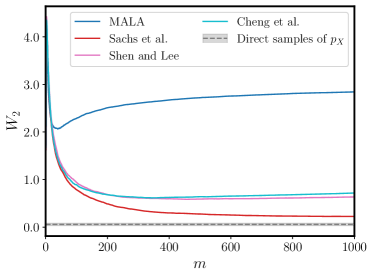
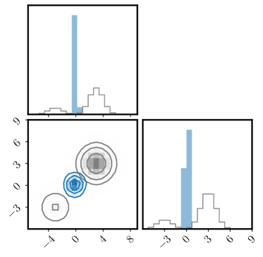
Refer to caption
Figure 5: W2subscript𝑊2W_{2} vs. m𝑚m for various MCMCσ algorithms used in the inner loop of Algorithm 1.
Refer to caption
(a) MALA (Roberts & Tweedie, 1996)
Refer to caption
(b) Cheng et al. (2018)
Refer to caption
(c) Shen & Lee (2019)
Refer to caption
(d) Sachs et al. (2017)
Figure 6: Final X^^𝑋\hat{X} samples for various MCMCσ algorithms used in the inner loop of Algorithm 1.

The algorithms are compared in Fig. 5 for the Gaussian mixture test density introduced in Sec. 5.2 with d=8𝑑8d=8. The three (unadjusted) ULD algorithms converge faster than does MALA to a lower W2subscript𝑊2W_{2}. In ULD algorithms, Brownian motion affects the positions xtsubscript𝑥𝑡x_{t} through the velocities vtsubscript𝑣𝑡v_{t}, rather than directly as in MALA, resulting in a smoother evolution of xtsubscript𝑥𝑡x_{t} that lends itself better to discretization. The first two dimensions of the final samples are displayed in Fig. 6. MALA samples fail to separate into the two modes, whereas Cheng et al, Shen and Lee, and Sachs et al have better sample quality, with Sachs et al performing the best and almost approaching the sample variance of W2subscript𝑊2W_{2} when samples are directly drawn from pXsubscript𝑝𝑋p_{X} (the gray band).

Refer to caption
(a) W2subscript𝑊2W_{2} vs. m𝑚m
Refer to caption
(b) Final W2subscript𝑊2W_{2} vs. number of MC samples
Figure 7: Effect of increasing the number of MC samples in the estimator of logp(y)𝑝𝑦\nabla\log p(y) for the mixture of Gaussians test density introduced in Sec. 5.2 with d=2𝑑2d=2
Refer to caption
(a) W2subscript𝑊2W_{2} vs. m𝑚m
Refer to caption
(b) Final W2subscript𝑊2W_{2} vs. number of MC samples
Figure 8: Effect of increasing the number of MC samples in the estimator of logp(y)𝑝𝑦\nabla\log p(y) for the mixture of Gaussians test density introduced in Sec. 5.2 with d=8𝑑8d=8

Appendix H Score estimation

Langevin MCMC requires the smoothed score function g(y;σ)=logp(y)𝑔𝑦𝜎𝑝𝑦g(y;\sigma)=\nabla\log p(y). Results presented earlier in Sec. 5 assumed access to the analytic score function. Here, we use the estimator presented in (4.9) with varying numbers of MC samples n𝑛n.

To prevent numerical underflow, we implemented (4.8) as follows:

A𝐴\displaystyle A =𝗅𝗈𝗀𝗌𝗎𝗆𝖾𝗑𝗉i=1n(f(y+σϵi)),absentsuperscriptsubscript𝗅𝗈𝗀𝗌𝗎𝗆𝖾𝗑𝗉𝑖1𝑛𝑓𝑦𝜎subscriptitalic-ϵ𝑖\displaystyle={\mathsf{logsumexp}}_{i=1}^{n}\bigl{(}-f(y+\sigma\epsilon_{i})\bigr{)}, (H.1)
B+subscript𝐵\displaystyle B_{+} =𝗅𝗈𝗀𝗌𝗎𝗆𝖾𝗑𝗉j=1n+(logϵjf(y+σϵj)),absentsuperscriptsubscript𝗅𝗈𝗀𝗌𝗎𝗆𝖾𝗑𝗉𝑗1subscript𝑛subscriptitalic-ϵ𝑗𝑓𝑦𝜎subscriptitalic-ϵ𝑗\displaystyle={\mathsf{logsumexp}}_{j=1}^{n_{+}}\bigl{(}\log\epsilon_{j}-f(y+\sigma\epsilon_{j})\bigr{)}, (H.2)
Bsubscript𝐵\displaystyle B_{-} =𝗅𝗈𝗀𝗌𝗎𝗆𝖾𝗑𝗉k=1n(logϵkf(y+σϵk)),absentsuperscriptsubscript𝗅𝗈𝗀𝗌𝗎𝗆𝖾𝗑𝗉𝑘1subscript𝑛subscriptitalic-ϵ𝑘𝑓𝑦𝜎subscriptitalic-ϵ𝑘\displaystyle={\mathsf{logsumexp}}_{k=1}^{n_{-}}\bigl{(}\log-\epsilon_{k}-f(y+\sigma\epsilon_{k})\bigr{)}, (H.3)
g^1(y;σ)subscript^𝑔1𝑦𝜎\displaystyle{\hat{g}}_{1}(y;\sigma) =1σ(eB+AeBA),absent1𝜎superscript𝑒subscript𝐵𝐴superscript𝑒subscript𝐵𝐴\displaystyle=\frac{1}{\sigma}\cdot\Bigl{(}e^{{B_{+}}-A}-e^{{B_{-}}-A}\Bigr{)}, (H.4)

where 𝗅𝗈𝗀𝗌𝗎𝗆𝖾𝗑𝗉i(ai)amax+logiexp(aiamax)subscript𝗅𝗈𝗀𝗌𝗎𝗆𝖾𝗑𝗉𝑖subscript𝑎𝑖subscript𝑎maxsubscript𝑖subscript𝑎𝑖subscript𝑎max{\mathsf{logsumexp}}_{i}(a_{i})\coloneqq a_{\rm max}+\log\sum_{i}\exp(a_{i}-a_{\rm max}) with amaxmaxiaisubscript𝑎maxsubscriptmax𝑖subscript𝑎𝑖a_{\rm max}\coloneqq{\rm max}_{i}\ a_{i}. In (H.2) and (H.3), j=1,,n+𝑗1subscript𝑛j=1,\dotsc,n_{+} and k=1,,n𝑘1subscript𝑛k=1,\dotsc,n_{-} denote the indices for which ϵitalic-ϵ\epsilon is positive and negative, respectively, with n++n=nsubscript𝑛subscript𝑛𝑛n_{+}+{n_{-}}=n. Note that the same Gaussian samples ϵitalic-ϵ\epsilon were used to evaluate the numerator and the denominator.

For a Gaussian mixture density introduced in Sec. 5.2 with d=2𝑑2d=2, both the analytic and the estimated score functions converge to a low W2subscript𝑊2W_{2}, as shown in Fig. 7. The sample quality is on par with the analytic score function with n𝑛n as small as 500 and there is little benefit to increasing the n𝑛n past 500.

For d=8𝑑8d=8, the estimated score reveals signs of error, as Fig. 8 shows. There is decreasing marginal return in W2subscript𝑊2W_{2} as n𝑛n doubles, although higher n𝑛n does help reduce W2subscript𝑊2W_{2} to some extent.

Variance reduction techniques, such as importance reweighting, may help get more mileage from finite n𝑛n.

Appendix I Mixture of correlated Gaussians

In this section, we study a correlated test density, namely a mixture of two 2-dimensional Gaussians with full covariances:

p(x)=α𝒩(x;μ,Σ0)+(1α)𝒩(x;μ,Σ1).𝑝𝑥𝛼𝒩𝑥𝜇subscriptΣ01𝛼𝒩𝑥𝜇subscriptΣ1p(x)=\alpha\,\mathcal{N}(x;\mu,\Sigma_{0})+(1-\alpha)\,\mathcal{N}(x;-\mu,\Sigma_{1}). (I.1)

We choose μ=31d𝜇3subscript1𝑑\mu=3\cdot 1_{d}, Σ0=Rdiag(14,4)RTsubscriptΣ0𝑅diag144superscript𝑅𝑇\Sigma_{0}=R\ {\rm diag}(\frac{1}{4},4)\ R^{T}, Σ1=RTdiag(1,9)RsubscriptΣ1superscript𝑅𝑇diag19𝑅\Sigma_{1}=R^{T}\ {\rm diag}(1,9)\ R, α=45𝛼45\alpha=\frac{4}{5}, and the rotation matrix

R=(cosθsinθsinθcosθ)𝑅matrix𝜃𝜃𝜃𝜃R=\begin{pmatrix}\cos\theta&-\sin\theta\\ \sin\theta&\cos\theta\end{pmatrix}

with θ=π/360𝜃𝜋360\theta=\pi/360. Fig. 9 compares the performance of the same Langevin MCMC algorithm (Sachs et al., 2017) used within the OAT scheme (a) with that used without Gaussian smoothing (b). In both cases here, we initialized the samplers at the origin (5000 particles total). The total number of iterations are the same between two algorithms (see Appendix F for details).
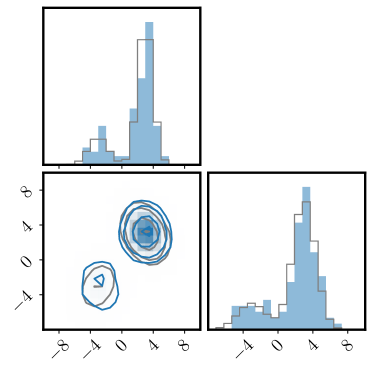
Refer to caption
(a) OAT, σ=16𝜎16\sigma=16, m=1000𝑚1000m=1000
Refer to caption
(b) Langevin MCMC
Figure 9: Mixture of correlated Gaussians.