A hierarchy of kinetic discrete-velocity models for traffic flow derived from a non-local Prigogine-Herman model

R. Borsche111Technische Universität Kaiserslautern, Department of Mathematics, Erwin-Schrödinger-Straße, 67663 Kaiserslautern, Germany ({borsche, klar}@mathematik.uni-kl.de)    A. Klar11footnotemark: 1 222Fraunhofer ITWM, Fraunhoferplatz 1, 67663 Kaiserslautern, Germany
Abstract

Starting from a non-local version of the Prigogine-Herman traffic model, we derive a natural hierarchy of kinetic discrete velocity models for traffic flow consisting of systems of quasi-linear hyperbolic equations with relaxation terms. The hyperbolic main part of these models turns out to have several favourable features. In particular, we determine Riemann invariants and prove richness and total linear degeneracy of the hyperbolic systems. Moreover, a physically reasonable invariant domain is obtained for all equations of the hierarchy. Additionally, we investigate the full relaxation system with respect to stability and persistence of periodic (stop and go type) solutions and derive a condition for the appearance of such solutions. Finally, numerical results for various situations are presented, illustrating the analytical findings.

Keywords. discrete-velocity model, traffic flow, relaxation system, rich and totally linear degenerate hyperbolic equation, persistent periodic waves.

AMS Classification. 90B20, 35L02, 35L04

1 Introduction and Motivation

Starting with the first macroscopic traffic model in [36], there have been many approaches to a continuous modeling of traffic flow problems. Macroscopic models are usually based on scalar hyperbolic equations like the above cited model or on systems of hyperbolic equations like in [30, 1, 37]. For discussions and extensions of these models see, for example, [2, 5, 4, 15, 34]. On the other hand, kinetic equations have also been widely used as a tool to model traffic flow problems. Starting with the work in [33] different extensions and amplifications can be found in [18, 22, 27, 29] or [21, 23]. For more recent works, we refer to [14] for a fully discrete kinetic approach, to [19] for a BGK-type traffic model, to [10, 11, 12, 7] for relations between kinetic and macroscopic models and to [3] for a mathematically oriented review and further references.

A naive use of classical kinetic equations in the case of traffic flow leads to well known problems: physically given invariant domains (a state space restricted to positive and bounded velocities and densities) are not respected and information transport against the flow direction is not possible. The second issue has been treated in several works introducing some additional mechanism into the equations. The Enskog type kinetic approaches in [21] use a non-locality to deal with these problem. Similarly, the discrete model developed in [14] includes the non-locality via a limiter term into the free flow part of the kinetic equation. The model in [19] uses a BGK-type approximation and a suitable modification to allow for a proper information transport.

In this work we derive a hierarchy of kinetic discrete velocity traffic models from a non-local version of the original Priogine-Herman kinetic traffic model [33]. In fluid- or gas-dynamics kinetic discrete velocity models have been investigated in many works, see [20] for a review. Consider as an example a classical continuous BGK-type kinetic equation for the kinetic distribution function f=f(x,v,t)0𝑓𝑓𝑥𝑣𝑡0f=f(x,v,t)\geq 0

tf+vxf=1ϵ(ffe(ρ,v))subscript𝑡𝑓𝑣subscript𝑥𝑓1italic-ϵ𝑓superscript𝑓𝑒𝜌𝑣\displaystyle\begin{aligned} \partial_{t}f+v\partial_{x}f=-\frac{1}{\epsilon}\left(f-f^{e}(\rho,v)\right)\end{aligned}

with f(v)𝑑v=ρ=fe(ρ,v)𝑑v𝑓𝑣differential-d𝑣𝜌superscript𝑓𝑒𝜌𝑣differential-d𝑣\int f(v)dv=\rho=\int f^{e}(\rho,v)dv. An associated discrete velocity model has the distribution functions fi,i=0,Nformulae-sequencesubscript𝑓𝑖𝑖0𝑁f_{i},i=0,\cdots N for velocities v0<v1<<vi<<vNsubscript𝑣0subscript𝑣1subscript𝑣𝑖subscript𝑣𝑁v_{0}<v_{1}<\cdots<v_{i}<\cdots<v_{N}. Let the discrete equilibrium functions be denoted by fie(ρ)subscriptsuperscript𝑓𝑒𝑖𝜌f^{e}_{i}(\rho), the density ρ𝜌\rho be given by ρ=f0++fN=f0e++fNe𝜌subscript𝑓0subscript𝑓𝑁subscriptsuperscript𝑓𝑒0subscriptsuperscript𝑓𝑒𝑁\rho=f_{0}+\cdots+f_{N}=f^{e}_{0}+\cdots+f^{e}_{N} and the mean flux by q=v0f0+v1f1++vNfN𝑞subscript𝑣0subscript𝑓0subscript𝑣1subscript𝑓1subscript𝑣𝑁subscript𝑓𝑁q=v_{0}f_{0}+v_{1}f_{1}+\cdots+v_{N}f_{N}. Then, with the equilibrium flux F(ρ)=v0f0e+v1f1e++vNfNe𝐹𝜌subscript𝑣0subscriptsuperscript𝑓𝑒0subscript𝑣1subscriptsuperscript𝑓𝑒1subscript𝑣𝑁subscriptsuperscript𝑓𝑒𝑁F(\rho)=v_{0}f^{e}_{0}+v_{1}f^{e}_{1}+\cdots+v_{N}f^{e}_{N}, the discrete-velocity model is given by

(1) tfi+vixfi=1ϵ(fifie(ρ)).subscript𝑡subscript𝑓𝑖subscript𝑣𝑖subscript𝑥subscript𝑓𝑖1italic-ϵsubscript𝑓𝑖subscriptsuperscript𝑓𝑒𝑖𝜌\displaystyle\begin{aligned} \partial_{t}f_{i}+v_{i}\partial_{x}f_{i}=-\frac{1}{\epsilon}\left(f_{i}-f^{e}_{i}(\rho)\right).\end{aligned}

The associated conservation law for the density for small values of ϵitalic-ϵ\epsilon is formally given by

tρ+xF(ρ)=0.subscript𝑡𝜌subscript𝑥𝐹𝜌0\partial_{t}\rho+\partial_{x}F(\rho)=0.

Applying this framework naively to traffic flow modeling, there are two simple observations related to each other. First, since in the traffic situation all velocities in the kinetic model are positive, i.e. vi0,i=0,,Nformulae-sequencesubscript𝑣𝑖0𝑖0𝑁v_{i}\geq 0,\;i=0,\ldots,N, there is no backward information transport, as, for example, in the case of a backward traveling traffic jam, since there are no negative wave speeds. The fact that there cannot be negative wave speeds also prevents a possible convergence to the limiting conservation law tρ+xF(ρ)=0,subscript𝑡𝜌subscript𝑥𝐹𝜌0\partial_{t}\rho+\partial_{x}F(\rho)=0, if there are situations with density ρ𝜌\rho, such that F(ρ)superscript𝐹𝜌F^{\prime}(\rho) is negative, due to the sub characteristic condition, see e.g. [26].

Second, since the density ρ𝜌\rho in a discrete velocity traffic model is limited by a maximal (bumper-to-bumper) density, the physically reasonable region for such a model is given by the N-simplex 0fi0subscript𝑓𝑖0\leq f_{i} and ρ=f0++fNρmax𝜌subscript𝑓0subscript𝑓𝑁subscript𝜌𝑚𝑎𝑥\rho=f_{0}+\cdots+f_{N}\leq\rho_{max}. However, this is not an invariant domain for the above equation (1). This can be easily seen looking at the hyperbolic part and considering a suitable Riemann problem. The bound on ρ𝜌\rho is not satisfied by the solutions of the equation and one obtains solutions with densities exceeding the bumper-to-bumper density. See the related discussion in [5] for macroscopic traffic models.

In the present paper we introduce a natural new class of discrete-velocity models for traffic flow derived from a non-local version of the classical Prigogine-Herman model and allowing a more rigorous investigation than previous approaches. To derive the equations we proceed similarly as in [6], where a strongly simplified relaxation model has been derived and investigated. It will turn out that the resulting model is a rich and totally linear degenerate system of hyperbolic equations with relaxation. Such systems have many favourable properties and have been studied in detail in the literature, see, for example, [32, 31, 25, 9]. Moreover, this class of discrete velocity models resolves the above issues: it is shown that the invariant region is given by the N-simplex discussed above and that the equations allow for negative wave speeds. Moreover, the full relaxation model exhibits stable and unstable flow situations allowing the modeling of stable traffic and of stop-and-go type instabilities in traffic flow.

Our starting point is a classical continuous kinetic traffic flow equation or, more exactly, a modified version of the spatially inhomogeneous original Prigogine-Herman equation. We proceed with a discretization in velocity space of these equations. A detailed investigation of the resulting hyperbolic parts of the equations of the discrete hierarchy gives a rich hyperbolic system and the invariant domain discussed above. Moreover, the equations together with the relaxation term are considered and a condition for stability respectively instability and appearance of persistent periodic (stop and go) waves is given following the approach in [16, 17]. See also [13] for a discussion of travelling wave solutions for macroscopic traffic equations.

The paper is organized in the following way. In section 2 we discuss a continuous kinetic traffic model based on the classical Prigogine Herman equation. In section 3 we derive a discrete velocity kinetic model from the continuous kinetic traffic equation. In the subsequent sections 4 and 5 the hyperbolic parts of the discrete kinetic equations are investigated in detail. In particular, we prove that the system is a rich and totally linear degenerate hyperbolic system. Section 6 discusses the full relaxation model and the above mentioned stability issues for continuous and discrete equations. Finally, numerical results are presented in Section 7.

2 A continuous kinetic model for traffic flow

Our starting point is a modified version of the classical kinetic Prigogine-Herman equation for traffic flow, see [21, 22, 23, 18, 27, 29, 33]. We proceed similarly as in [6].

2.1 Derivation of the continuous kinetic model

The kinetic model is based on an underlying microscopic model with breaking interactions, where the driver at x𝑥x with velocity v𝑣v reacts to his predecessor at x+H𝑥𝐻x+H with velocity v^<v^𝑣𝑣\hat{v}<v. Here H>0𝐻0H>0 is a minimal distance between the vehicles. The new velocity resulting of this braking interaction is equal to the velocity of the leading car. Then, 1H1𝐻\frac{1}{H} is the maximal density of vehicles on the road and the interaction strength is modulated by a factor 11Hρ11𝐻𝜌\frac{1}{1-H\rho} which can be derived from the two particle correlation function of the vehicles, compare [23]. One obtains for t+𝑡superscriptt\in\mathbb{R}^{+}, x𝑥x\in\mathbb{R}, v[0,vmax]𝑣0subscript𝑣𝑚𝑎𝑥v\in[0,v_{max}] the following equation for the distribution function f=f(x,v,t)0𝑓𝑓𝑥𝑣𝑡0f=f(x,v,t)\geq 0

tf+vxf=J(f)=JB(f)+JA(f),subscript𝑡𝑓𝑣subscript𝑥𝑓𝐽𝑓subscript𝐽𝐵𝑓subscript𝐽𝐴𝑓\displaystyle\partial_{t}f+v\partial_{x}f=J(f)=J_{B}(f)+J_{A}(f),

where JBsubscript𝐽𝐵J_{B} describes the interactions with respect to braking and JAsubscript𝐽𝐴J_{A} additional interactions, like those related to acceleration. The braking term JB(f)subscript𝐽𝐵𝑓J_{B}(f) is given as in [33, 8] by

JB(f)=11Hρv^>v(v^v)f(x,v^)f(x+H,v)𝑑v^subscript𝐽𝐵𝑓11𝐻𝜌subscript^𝑣𝑣^𝑣𝑣𝑓𝑥^𝑣𝑓𝑥𝐻𝑣differential-d^𝑣\displaystyle J_{B}(f)=\frac{1}{1-H\rho}\int_{\hat{v}>v}(\hat{v}-v)f(x,\hat{v})f(x+H,v)d\hat{v}
11Hρv^<v(vv^)f(x,v)f(x+H,v^)𝑑v^11𝐻𝜌subscript^𝑣𝑣𝑣^𝑣𝑓𝑥𝑣𝑓𝑥𝐻^𝑣differential-d^𝑣\displaystyle-\frac{1}{1-H\rho}\int_{\hat{v}<v}(v-\hat{v})f(x,v)f(x+H,\hat{v})d\hat{v}\

with ρ=0vmaxf(v)𝑑vρmax=1H𝜌superscriptsubscript0subscript𝑣𝑚𝑎𝑥𝑓𝑣differential-d𝑣subscript𝜌𝑚𝑎𝑥1𝐻\rho=\int_{0}^{v_{max}}f(v)dv\leq\rho_{max}=\frac{1}{H}.

Nondimensionalization using the new variables x~=xH,t~=vmaxHtformulae-sequence~𝑥𝑥𝐻~𝑡subscript𝑣𝑚𝑎𝑥𝐻𝑡\tilde{x}=\frac{x}{H},\tilde{t}=\frac{v_{max}}{H}t, v~=vvmax~𝑣𝑣subscript𝑣𝑚𝑎𝑥\tilde{v}=\frac{v}{v_{max}} and the new distribution function f~(x~,v~,t~)=vmaxρmaxf(x,v,t)=Hvmaxf(x,v,t)~𝑓~𝑥~𝑣~𝑡subscript𝑣𝑚𝑎𝑥subscript𝜌𝑚𝑎𝑥𝑓𝑥𝑣𝑡𝐻subscript𝑣𝑚𝑎𝑥𝑓𝑥𝑣𝑡\tilde{f}(\tilde{x},\tilde{v},\tilde{t})=\frac{v_{max}}{\rho_{max}}f(x,v,t)=Hv_{max}f(x,v,t) gives, if we neglect the tilde-notation, the equation

(2) tf+vxf=JB(f)+JA(f)subscript𝑡𝑓𝑣subscript𝑥𝑓subscript𝐽𝐵𝑓subscript𝐽𝐴𝑓\displaystyle\partial_{t}f+v\partial_{x}f=J_{B}(f)+J_{A}(f)

with

JB(f)=11ρv^>v(v^v)f(x,v^)f(x+1,v)𝑑v^subscript𝐽𝐵𝑓11𝜌subscript^𝑣𝑣^𝑣𝑣𝑓𝑥^𝑣𝑓𝑥1𝑣differential-d^𝑣\displaystyle J_{B}(f)=\frac{1}{1-\rho}\int_{\hat{v}>v}(\hat{v}-v)f(x,\hat{v})f(x+1,v)d\hat{v}
11ρv^<v(vv^)f(x,v)f(x+1,v^)𝑑v^,11𝜌subscript^𝑣𝑣𝑣^𝑣𝑓𝑥𝑣𝑓𝑥1^𝑣differential-d^𝑣\displaystyle-\frac{1}{1-\rho}\int_{\hat{v}<v}(v-\hat{v})f(x,v)f(x+1,\hat{v})d\hat{v}\ ,

where t+𝑡superscriptt\in\mathbb{R}^{+}, x𝑥x\in\mathbb{R}, v[0,1]𝑣01v\in[0,1] and ρ=01f(v)𝑑v1𝜌superscriptsubscript01𝑓𝑣differential-d𝑣1\rho=\int_{0}^{1}f(v)dv\leq 1.

Now, we split the braking term into two terms containing the local and non-local braking effects, respectively. The local braking term is

JBL(f)superscriptsubscript𝐽𝐵𝐿𝑓\displaystyle J_{B}^{L}(f) =11ρv^>v(v^v)f(x,v^)f(x,v)𝑑v^absent11𝜌subscript^𝑣𝑣^𝑣𝑣𝑓𝑥^𝑣𝑓𝑥𝑣differential-d^𝑣\displaystyle=\frac{1}{1-\rho}\int_{\hat{v}>v}(\hat{v}-v)f(x,\hat{v})f(x,v)d\hat{v}
11ρv^<v(vv^)f(x,v)f(x,v^)𝑑v^11𝜌subscript^𝑣𝑣𝑣^𝑣𝑓𝑥𝑣𝑓𝑥^𝑣differential-d^𝑣\displaystyle-\frac{1}{1-\rho}\int_{\hat{v}<v}(v-\hat{v})f(x,v)f(x,\hat{v})d\hat{v}
=11ρ(v^v)f(v)f(v^)𝑑v^=f(v)qvρ1ρabsent11𝜌^𝑣𝑣𝑓𝑣𝑓^𝑣differential-d^𝑣𝑓𝑣𝑞𝑣𝜌1𝜌\displaystyle=\frac{1}{1-\rho}\int(\hat{v}-v)f(v)f(\hat{v})d\hat{v}=f(v)\frac{q-v\rho}{1-\rho}

with q=01vf(v)𝑑v𝑞superscriptsubscript01𝑣𝑓𝑣differential-d𝑣q=\int_{0}^{1}vf(v)dv.

Remark 1.

The term JBLsuperscriptsubscript𝐽𝐵𝐿J_{B}^{L} is the classical breaking term for kinetic problems as in the work of Prigogine and Herman [33].

The term containing the non-local effects due to braking interactions is then denoted by JBNL(f)superscriptsubscript𝐽𝐵𝑁𝐿𝑓J_{B}^{NL}(f). Thus,

JBNL(f)=JB(f)JBL(f).superscriptsubscript𝐽𝐵𝑁𝐿𝑓subscript𝐽𝐵𝑓superscriptsubscript𝐽𝐵𝐿𝑓J_{B}^{NL}(f)=J_{B}(f)-J_{B}^{L}(f).

The total local effects are then described by the combined term

JL(f)=JA(f)+JBL(f).superscript𝐽𝐿𝑓subscript𝐽𝐴𝑓superscriptsubscript𝐽𝐵𝐿𝑓\displaystyle J^{L}(f)=J_{A}(f)+J_{B}^{L}(f).

To simplify the situation we approximate this term by a standard relaxation term

JL(f)JR(f)=1T(ffe(ρ,v))superscript𝐽𝐿𝑓subscript𝐽𝑅𝑓1𝑇𝑓superscript𝑓𝑒𝜌𝑣\displaystyle J^{L}(f)\approx J_{R}(f)=-\frac{1}{T}\left(f-f^{e}(\rho,v)\right)\

with an equilibrium function fesuperscript𝑓𝑒f^{e} fulfilling fe(ρ,v)𝑑v=ρ=f(v)𝑑vsuperscript𝑓𝑒𝜌𝑣differential-d𝑣𝜌𝑓𝑣differential-d𝑣\int f^{e}(\rho,v)dv=\rho=\int f(v)dv. The first moment of fesuperscript𝑓𝑒f^{e} is vfe(ρ,v)𝑑v=F(ρ)𝑣superscript𝑓𝑒𝜌𝑣differential-d𝑣𝐹𝜌\int vf^{e}(\rho,v)dv=F(\rho), where F(ρ),0ρ1𝐹𝜌0𝜌1F(\rho),0\leq\rho\leq 1 is called the fundamental diagram. fesuperscript𝑓𝑒f^{e} is chosen in such a way, that V(ρ)=F(ρ)ρ𝑉𝜌𝐹𝜌𝜌V(\rho)=\frac{F(\rho)}{\rho} is monotone decaying with V(0)=1𝑉01V(0)=1 and V(1)=0𝑉10V(1)=0. This yields functions F𝐹F fulfilling F(0)=F(1)=0𝐹0𝐹10F(0)=F(1)=0 and F(ρ)1superscript𝐹𝜌1F^{\prime}(\rho)\leq 1. Moreover, in the following, we use E=E(ρ)𝐸𝐸𝜌E=E(\rho) to denote the second moment of fesuperscript𝑓𝑒f^{e}, i.e. E=v2fe(ρ,v)𝑑v𝐸superscript𝑣2superscript𝑓𝑒𝜌𝑣differential-d𝑣E=\int v^{2}f^{e}(\rho,v)dv.

Example 1.

As an example for the equilibrium function fesuperscript𝑓𝑒f^{e}, which will also be used for numerical computations, we consider a class of equilibrium functions fesuperscript𝑓𝑒f^{e} depending only on the first 3 moments ρ,F,E𝜌𝐹𝐸\rho,F,E, i.e.

fe(ρ,v)=δ0(v)(ρF(γ1)FE1λ)+FE1λg(v)v+δ1(v)(FFE1λ)superscript𝑓𝑒𝜌𝑣subscript𝛿0𝑣𝜌𝐹𝛾1𝐹𝐸1𝜆𝐹𝐸1𝜆𝑔𝑣𝑣subscript𝛿1𝑣𝐹𝐹𝐸1𝜆\displaystyle f^{e}(\rho,v)=\delta_{0}(v)\left(\rho-F-(\gamma-1)\frac{F-E}{1-\lambda}\right)+\frac{F-E}{1-\lambda}\frac{g(v)}{v}+\delta_{1}(v)\left(F-\frac{F-E}{1-\lambda}\right)

with a smooth function g0𝑔0g\geq 0, 01g(v)𝑑v=1superscriptsubscript01𝑔𝑣differential-d𝑣1\int_{0}^{1}g(v)dv=1. Here λ=01vg(v)𝑑v𝜆superscriptsubscript01𝑣𝑔𝑣differential-d𝑣\lambda=\int_{0}^{1}vg(v)dv and we require γ=01g(v)v𝑑v<𝛾superscriptsubscript01𝑔𝑣𝑣differential-d𝑣\gamma=\int_{0}^{1}\frac{g(v)}{v}dv<\infty. Note that realizability, i.e. positivity of fesuperscript𝑓𝑒f^{e}, requires

(3) F1λγ1(ρF)EandλFEF𝐹1𝜆𝛾1𝜌𝐹𝐸and𝜆𝐹𝐸𝐹\displaystyle F-\frac{1-\lambda}{\gamma-1}(\rho-F)\leq E\;\mbox{and}\;\lambda F\leq E\leq F

for all 0<ρ<10𝜌10<\rho<1.

To continue, the kinetic equation is now scaled with a hyperbolic space time scaling ttϵ𝑡𝑡italic-ϵt\rightarrow\frac{t}{\epsilon} and xxϵ𝑥𝑥italic-ϵx\rightarrow\frac{x}{\epsilon}. This leads to

tf+vxf=1ϵJR(f)+1ϵJBNL(f)subscript𝑡𝑓𝑣subscript𝑥𝑓1italic-ϵsubscript𝐽𝑅𝑓1italic-ϵsuperscriptsubscript𝐽𝐵𝑁𝐿𝑓\displaystyle\partial_{t}f+v\partial_{x}f=\frac{1}{\epsilon}J_{R}(f)+\frac{1}{\epsilon}J_{B}^{NL}(f)

with

JBNL(f)superscriptsubscript𝐽𝐵𝑁𝐿𝑓\displaystyle J_{B}^{NL}(f) =11ρv^>v(v^v)f(x,v^)[f(x+ϵ,v)f(x,v)]𝑑v^absent11𝜌subscript^𝑣𝑣^𝑣𝑣𝑓𝑥^𝑣delimited-[]𝑓𝑥italic-ϵ𝑣𝑓𝑥𝑣differential-d^𝑣\displaystyle=\frac{1}{1-\rho}\int_{\hat{v}>v}(\hat{v}-v)f(x,\hat{v})[f(x+\epsilon,v)-f(x,v)]d\hat{v}
11ρv^<v(vv^)f(x,v)[f(x+ϵ,v^)f(x,v^)]𝑑v^.11𝜌subscript^𝑣𝑣𝑣^𝑣𝑓𝑥𝑣delimited-[]𝑓𝑥italic-ϵ^𝑣𝑓𝑥^𝑣differential-d^𝑣\displaystyle-\frac{1}{1-\rho}\int_{\hat{v}<v}(v-\hat{v})f(x,v)[f(x+\epsilon,\hat{v})-f(x,\hat{v})]d\hat{v}.
Remark 2.

Note that in the fluid dynamic context, this is the classical hydrodynamic Enskog-Boltzmann scaling, see, for example, [24].

Using a Taylor approximation we approximate the non-local term to order 𝒪(ϵ2)𝒪superscriptitalic-ϵ2\mathcal{O}(\epsilon^{2}) by the term ϵJ(f,xf)italic-ϵ𝐽𝑓subscript𝑥𝑓\epsilon J(f,\partial_{x}f) with

J(f,xf)=11ρv^>v(v^v)f(v^)xf(v)dv^11ρv^<v(vv^)f(v)xf(v^)dv^.𝐽𝑓subscript𝑥𝑓11𝜌subscript^𝑣𝑣^𝑣𝑣𝑓^𝑣subscript𝑥𝑓𝑣𝑑^𝑣11𝜌subscript^𝑣𝑣𝑣^𝑣𝑓𝑣subscript𝑥𝑓^𝑣𝑑^𝑣\displaystyle J(f,\partial_{x}f)=\frac{1}{1-\rho}\int_{\hat{v}>v}(\hat{v}-v)f(\hat{v})\partial_{x}f(v)d\hat{v}-\frac{1}{1-\rho}\int_{\hat{v}<v}(v-\hat{v})f(v)\partial_{x}f(\hat{v})d\hat{v}\ .

Altogether, we obtain the kinetic problem

(4) tf+vxfJ(f,xf)=1ϵJR(f),subscript𝑡𝑓𝑣subscript𝑥𝑓𝐽𝑓subscript𝑥𝑓1italic-ϵsubscript𝐽𝑅𝑓\displaystyle\partial_{t}f+v\partial_{x}f-J(f,\partial_{x}f)=\frac{1}{\epsilon}J_{R}(f),

which will be the starting point of our investigations.

3 Discrete velocity models for traffic flow

To obtain a hierarchy of discrete velocity models we discretize equation (4) in velocity space with the (not necessarily equidistant) velocities 0=v0<v1<v2<<vN1<vN=10subscript𝑣0subscript𝑣1subscript𝑣2subscript𝑣𝑁1subscript𝑣𝑁10=v_{0}<v_{1}<v_{2}<\cdots<v_{N-1}<v_{N}=1. Note that the choices v0=0subscript𝑣00v_{0}=0 and vN=1subscript𝑣𝑁1v_{N}=1 are necessary to span the full range of all possible velocities. The associated discrete distribution functions we denote fi=fi(x,t)[0,1],i=0,,Nformulae-sequencesubscript𝑓𝑖subscript𝑓𝑖𝑥𝑡01𝑖0𝑁f_{i}=f_{i}(x,t)\in[0,1],i=0,\ldots,N and define the discrete density and momentum by

ρ=i=0Nfiandq=i=0Nvifi.formulae-sequence𝜌superscriptsubscript𝑖0𝑁subscript𝑓𝑖and𝑞superscriptsubscript𝑖0𝑁subscript𝑣𝑖subscript𝑓𝑖\displaystyle\rho=\sum_{i=0}^{N}f_{i}\qquad\mbox{and}\qquad q=\sum_{i=0}^{N}v_{i}f_{i}.

For the discretization of the equilibrium distribution we use discrete values fie(ρ)subscriptsuperscript𝑓𝑒𝑖𝜌f^{e}_{i}(\rho), i=0,,N𝑖0𝑁i=0,\ldots,N fulfilling i=0Nfie(ρ)=ρsuperscriptsubscript𝑖0𝑁subscriptsuperscript𝑓𝑒𝑖𝜌𝜌\sum_{i=0}^{N}f^{e}_{i}(\rho)=\rho and denote again i=0Nvifie(ρ)=F(ρ).superscriptsubscript𝑖0𝑁subscript𝑣𝑖subscriptsuperscript𝑓𝑒𝑖𝜌𝐹𝜌\sum_{i=0}^{N}v_{i}f^{e}_{i}(\rho)=F(\rho).

We obtain the following discretization of the term (1ρ)J(f,xf)1𝜌𝐽𝑓subscript𝑥𝑓(1-\rho)J(f,\partial_{x}f).

i=0::𝑖0absent\displaystyle i=0: j=1Nvjfjxf0superscriptsubscript𝑗1𝑁subscript𝑣𝑗subscript𝑓𝑗subscript𝑥subscript𝑓0\displaystyle\;\sum_{j=1}^{N}v_{j}f_{j}\partial_{x}f_{0}
i=1,,N1::𝑖1𝑁1absent\displaystyle i=1,\ldots,N-1: j=i+1N(vjvi)fjxfij=0i1(vivj)fixfjsuperscriptsubscript𝑗𝑖1𝑁subscript𝑣𝑗subscript𝑣𝑖subscript𝑓𝑗subscript𝑥subscript𝑓𝑖superscriptsubscript𝑗0𝑖1subscript𝑣𝑖subscript𝑣𝑗subscript𝑓𝑖subscript𝑥subscript𝑓𝑗\displaystyle\;\sum_{j=i+1}^{N}(v_{j}-v_{i})f_{j}\partial_{x}f_{i}-\sum_{j=0}^{i-1}(v_{i}-v_{j})f_{i}\partial_{x}f_{j}
i=N::𝑖𝑁absent\displaystyle i=N: j=0N1(1vj)fNxfj.superscriptsubscript𝑗0𝑁11subscript𝑣𝑗subscript𝑓𝑁subscript𝑥subscript𝑓𝑗\displaystyle\;-\sum_{j=0}^{N-1}(1-v_{j})f_{N}\partial_{x}f_{j}.

Altogether, this gives the hyperbolic system

(5) tf0+v0xf011ρ[j=1N(vjv0)fjxf0]=JR0tfi+vixfi11ρ[j=i+1N(vjvi)fjxfij=0i1(vivj)fixfj]=JRitfN+vNxfN11ρ[j=0N1(vNvj)fNxfj]=JRNsubscript𝑡subscript𝑓0subscript𝑣0subscript𝑥subscript𝑓011𝜌delimited-[]superscriptsubscript𝑗1𝑁subscript𝑣𝑗subscript𝑣0subscript𝑓𝑗subscript𝑥subscript𝑓0superscriptsubscript𝐽𝑅0subscript𝑡subscript𝑓𝑖subscript𝑣𝑖subscript𝑥subscript𝑓𝑖11𝜌delimited-[]superscriptsubscript𝑗𝑖1𝑁subscript𝑣𝑗subscript𝑣𝑖subscript𝑓𝑗subscript𝑥subscript𝑓𝑖superscriptsubscript𝑗0𝑖1subscript𝑣𝑖subscript𝑣𝑗subscript𝑓𝑖subscript𝑥subscript𝑓𝑗superscriptsubscript𝐽𝑅𝑖subscript𝑡subscript𝑓𝑁subscript𝑣𝑁subscript𝑥subscript𝑓𝑁11𝜌delimited-[]superscriptsubscript𝑗0𝑁1subscript𝑣𝑁subscript𝑣𝑗subscript𝑓𝑁subscript𝑥subscript𝑓𝑗superscriptsubscript𝐽𝑅𝑁\displaystyle\begin{aligned} \partial_{t}f_{0}+v_{0}\partial_{x}f_{0}-\frac{1}{1-\rho}\left[\sum_{j=1}^{N}(v_{j}-v_{0})f_{j}\partial_{x}f_{0}\right]=J_{R}^{0}\\ \partial_{t}f_{i}+v_{i}\partial_{x}f_{i}-\frac{1}{1-\rho}\left[\sum_{j=i+1}^{N}(v_{j}-v_{i})f_{j}\partial_{x}f_{i}-\sum_{j=0}^{i-1}(v_{i}-v_{j})f_{i}\partial_{x}f_{j}\right]=J_{R}^{i}\\ \partial_{t}f_{N}+v_{N}\partial_{x}f_{N}-\frac{1}{1-\rho}\left[-\sum_{j=0}^{N-1}(v_{N}-v_{j})f_{N}\partial_{x}f_{j}\right]=J_{R}^{N}\end{aligned}

for i=1,,N1𝑖1𝑁1i=1,\ldots,N-1. Here

JRi=1T(fifie(ρ))superscriptsubscript𝐽𝑅𝑖1𝑇subscript𝑓𝑖subscriptsuperscript𝑓𝑒𝑖𝜌\displaystyle J_{R}^{i}=-\frac{1}{T}(f_{i}-f^{e}_{i}(\rho))

for i=0,,N𝑖0𝑁i=0,\ldots,N. This is a quasilinear hyperbolic system

tf+A(f)xf=JR(f),subscript𝑡𝑓𝐴𝑓subscript𝑥𝑓subscript𝐽𝑅𝑓\partial_{t}f+A(f)\partial_{x}f=J_{R}(f),

where the lower triangular matrix has the values

Aii(f)=vi11ρ(j=i+1N(vjvi)fj),Aij(f)=11ρ(vivj)fi0 for j<i.formulae-sequencesubscript𝐴𝑖𝑖𝑓subscript𝑣𝑖11𝜌superscriptsubscript𝑗𝑖1𝑁subscript𝑣𝑗subscript𝑣𝑖subscript𝑓𝑗subscript𝐴𝑖𝑗𝑓11𝜌subscript𝑣𝑖subscript𝑣𝑗subscript𝑓𝑖0 for 𝑗𝑖\displaystyle A_{ii}(f)=v_{i}-\frac{1}{1-\rho}\left(\sum_{j=i+1}^{N}(v_{j}-v_{i})f_{j}\right)\ ,\quad A_{ij}(f)=\frac{1}{1-\rho}(v_{i}-v_{j})f_{i}\geq 0\text{ for }j<i.

The eigenvalues of A𝐴A are

λ0subscript𝜆0\displaystyle\lambda_{0} =11ρj=1Nvjfj0,absent11𝜌superscriptsubscript𝑗1𝑁subscript𝑣𝑗subscript𝑓𝑗0\displaystyle=-\frac{1}{1-\rho}\sum_{j=1}^{N}v_{j}f_{j}\leq 0, λN=1,subscript𝜆𝑁1\displaystyle\lambda_{N}=1,
λisubscript𝜆𝑖\displaystyle\lambda_{i} =vi11ρj=i+1N(vjvi)fj,absentsubscript𝑣𝑖11𝜌superscriptsubscript𝑗𝑖1𝑁subscript𝑣𝑗subscript𝑣𝑖subscript𝑓𝑗\displaystyle=v_{i}-\frac{1}{1-\rho}\sum_{j=i+1}^{N}(v_{j}-v_{i})f_{j}, i=1,,N1𝑖1𝑁1\displaystyle i=1,\ldots,N-1
Example 2.

N=1𝑁1N=1. For a two velocity model with the velocities 0=v0,v1=1formulae-sequence0subscript𝑣0subscript𝑣110=v_{0},v_{1}=1 we obtain

tf011ρf1xf0subscript𝑡subscript𝑓011𝜌subscript𝑓1subscript𝑥subscript𝑓0\displaystyle\partial_{t}f_{0}-\frac{1}{1-\rho}f_{1}\partial_{x}f_{0} =1ϵ(f0ρ+F(ρ))absent1italic-ϵsubscript𝑓0𝜌𝐹𝜌\displaystyle=-\frac{1}{\epsilon}\left(f_{0}-\rho+F(\rho)\right)
tf1+xf1+11ρf1xf0subscript𝑡subscript𝑓1subscript𝑥subscript𝑓111𝜌subscript𝑓1subscript𝑥subscript𝑓0\displaystyle\partial_{t}f_{1}+\partial_{x}f_{1}+\frac{1}{1-\rho}f_{1}\partial_{x}f_{0} =1ϵ(f1F(ρ)).absent1italic-ϵsubscript𝑓1𝐹𝜌\displaystyle=-\frac{1}{\epsilon}\left(f_{1}-F(\rho)\right).

Note that this is the simplified relaxation model derived in [6].

Example 3.

N=2𝑁2N=2. For the three velocity model we obtain with ρ=f0+f1+f2𝜌subscript𝑓0subscript𝑓1subscript𝑓2\rho=f_{0}+f_{1}+f_{2} and q=v1f1+f2𝑞subscript𝑣1subscript𝑓1subscript𝑓2q=v_{1}f_{1}+f_{2} and e=v12f1+f2𝑒superscriptsubscript𝑣12subscript𝑓1subscript𝑓2e=v_{1}^{2}f_{1}+f_{2} and E(ρ)=v12f1e+f2e𝐸𝜌superscriptsubscript𝑣12subscriptsuperscript𝑓𝑒1subscriptsuperscript𝑓𝑒2E(\rho)=v_{1}^{2}f^{e}_{1}+f^{e}_{2}, the following expressions f0=ρf1f2subscript𝑓0𝜌subscript𝑓1subscript𝑓2f_{0}=\rho-f_{1}-f_{2}, f1=qev1(1v1)subscript𝑓1𝑞𝑒subscript𝑣11subscript𝑣1f_{1}=\frac{q-e}{v_{1}(1-v_{1})}, f2=ev1q1v1subscript𝑓2𝑒subscript𝑣1𝑞1subscript𝑣1f_{2}=\frac{e-v_{1}q}{1-v_{1}} and

tf0q1ρxf0subscript𝑡subscript𝑓0𝑞1𝜌subscript𝑥subscript𝑓0\displaystyle\partial_{t}f_{0}-\frac{q}{1-\rho}\partial_{x}f_{0} =1ϵ(f0ρ+(1v12)F(ρ)E(ρ)(1v1))v1(1v1))\displaystyle=-\frac{1}{\epsilon}\left(f_{0}-\rho+\frac{(1-v_{1}^{2})F(\rho)-E(\rho)(1-v_{1}))}{v_{1}(1-v_{1})}\right)
tf1+(v11v11ρf2)xf1subscript𝑡subscript𝑓1subscript𝑣11subscript𝑣11𝜌subscript𝑓2subscript𝑥subscript𝑓1\displaystyle\partial_{t}f_{1}+\left(v_{1}-\frac{1-v_{1}}{1-\rho}f_{2}\right)\partial_{x}f_{1} +v11ρf1xf0=1ϵ(f1F(ρ)E(ρ)v1(1v1))subscript𝑣11𝜌subscript𝑓1subscript𝑥subscript𝑓01italic-ϵsubscript𝑓1𝐹𝜌𝐸𝜌subscript𝑣11subscript𝑣1\displaystyle+\frac{v_{1}}{1-\rho}f_{1}\partial_{x}f_{0}=-\frac{1}{\epsilon}\left(f_{1}-\frac{F(\rho)-E(\rho)}{v_{1}(1-v_{1})}\right)
tf2+xf2+1v11ρf2xf1subscript𝑡subscript𝑓2subscript𝑥subscript𝑓21subscript𝑣11𝜌subscript𝑓2subscript𝑥subscript𝑓1\displaystyle\partial_{t}f_{2}+\partial_{x}f_{2}+\frac{1-v_{1}}{1-\rho}f_{2}\partial_{x}f_{1} +11ρf2xf0=1ϵ(f2v1E(ρ)v12F(ρ)v1(1v1))).\displaystyle+\frac{1}{1-\rho}f_{2}\partial_{x}f_{0}=-\frac{1}{\epsilon}\left(f_{2}-\frac{v_{1}E(\rho)-v_{1}^{2}F(\rho)}{v_{1}(1-v_{1})})\right).

Suitable functions for F𝐹F and E𝐸E lie in the realizability region

(6) Fv1(ρF)E,v1FEF.formulae-sequence𝐹subscript𝑣1𝜌𝐹𝐸subscript𝑣1𝐹𝐸𝐹\displaystyle F-v_{1}(\rho-F)\leq E,\;v_{1}F\leq E\leq F.

Example 4.

General N𝑁N. We obtain an example for general N𝑁N via considering a discrete version of the equilibrium distribution in Example 1. That means we consider equilibrium functions of the following form. Fix a function F=F(ρ)𝐹𝐹𝜌F=F(\rho) and E=E(ρ)𝐸𝐸𝜌E=E(\rho). Moreover, let 0αi1,i=1,,N1formulae-sequence0subscript𝛼𝑖1𝑖1𝑁10\leq\alpha_{i}\leq 1,i=1,\ldots,N-1 and i=1N1αi=1superscriptsubscript𝑖1𝑁1subscript𝛼𝑖1\sum_{i=1}^{N-1}\alpha_{i}=1. Moreover, we define λ=i=1N1αivi𝜆superscriptsubscript𝑖1𝑁1subscript𝛼𝑖subscript𝑣𝑖\lambda=\sum_{i=1}^{N-1}\alpha_{i}v_{i} and γ=i=1N1αivi𝛾superscriptsubscript𝑖1𝑁1subscript𝛼𝑖subscript𝑣𝑖\gamma=\sum_{i=1}^{N-1}\frac{\alpha_{i}}{v_{i}}. Then

fie(ρ,v)superscriptsubscript𝑓𝑖𝑒𝜌𝑣\displaystyle f_{i}^{e}(\rho,v) =αiviFE1λ,absentsubscript𝛼𝑖subscript𝑣𝑖𝐹𝐸1𝜆\displaystyle=\frac{\alpha_{i}}{v_{i}}\frac{F-E}{1-\lambda}, i=1,,N1,𝑖1𝑁1\displaystyle i=1,\ldots,N-1,
fNe(ρ,v)superscriptsubscript𝑓𝑁𝑒𝜌𝑣\displaystyle f_{N}^{e}(\rho,v) =Fi=1N1vifie,absent𝐹superscriptsubscript𝑖1𝑁1subscript𝑣𝑖superscriptsubscript𝑓𝑖𝑒\displaystyle=F-\sum_{i=1}^{N-1}v_{i}f_{i}^{e}\ , f0e(ρ,v)=ρi=1Nfiesuperscriptsubscript𝑓0𝑒𝜌𝑣𝜌superscriptsubscript𝑖1𝑁superscriptsubscript𝑓𝑖𝑒\displaystyle f_{0}^{e}(\rho,v)=\rho-\sum_{i=1}^{N}f_{i}^{e}

Realizability requires again F1λγ1(ρF)E𝐹1𝜆𝛾1𝜌𝐹𝐸F-\frac{1-\lambda}{\gamma-1}(\rho-F)\leq E and λFEF𝜆𝐹𝐸𝐹\lambda F\leq E\leq F for all 0<ρ<10𝜌10<\rho<1 as in the continuous case. Note that for N=2𝑁2N=2 this is Example 3.

4 Properties of the hyperbolic model

In this and the following section we will give a thorough discussion of the hyperbolic part of (5) and show that the hyperbolic systems are, for all values of N𝑁N, rich and totally linear degenerate, which leads to global existence of solutions, see [31, 32]. We start with investigating the properties of the eigenvalues and eigenvectors of the system matrix. Obviously λN=0subscript𝜆𝑁0\nabla\lambda_{N}=0 and for i=0,,N1𝑖0𝑁1i=0,\ldots,N-1 we have with α=11ρ𝛼11𝜌\alpha=\frac{1}{1-\rho}

λi=(1(1ρ)2j=i+1N(vjvi)fj1(1ρ)2j=i+1N(vjvi)fj11ρ(vi+1vi)1(1ρ)2j=i+1N(vjvi)fj11ρ(vkvi)1(1ρ)2j=i+1N(vjvi)fjH1ρ(vNvi)1(1ρ)2j=i+1N(vjvi)fj)=α(λiviλiviλivi+1λivkλivN).subscript𝜆𝑖matrix1superscript1𝜌2superscriptsubscript𝑗𝑖1𝑁subscript𝑣𝑗subscript𝑣𝑖subscript𝑓𝑗1superscript1𝜌2superscriptsubscript𝑗𝑖1𝑁subscript𝑣𝑗subscript𝑣𝑖subscript𝑓𝑗11𝜌subscript𝑣𝑖1subscript𝑣𝑖1superscript1𝜌2superscriptsubscript𝑗𝑖1𝑁subscript𝑣𝑗subscript𝑣𝑖subscript𝑓𝑗11𝜌subscript𝑣𝑘subscript𝑣𝑖1superscript1𝜌2superscriptsubscript𝑗𝑖1𝑁subscript𝑣𝑗subscript𝑣𝑖subscript𝑓𝑗𝐻1𝜌subscript𝑣𝑁subscript𝑣𝑖1superscript1𝜌2superscriptsubscript𝑗𝑖1𝑁subscript𝑣𝑗subscript𝑣𝑖subscript𝑓𝑗𝛼matrixsubscript𝜆𝑖subscript𝑣𝑖subscript𝜆𝑖subscript𝑣𝑖subscript𝜆𝑖subscript𝑣𝑖1subscript𝜆𝑖subscript𝑣𝑘subscript𝜆𝑖subscript𝑣𝑁\displaystyle\nabla\lambda_{i}=\left(\begin{matrix}-\frac{1}{(1-\rho)^{2}}\sum_{j=i+1}^{N}(v_{j}-v_{i})f_{j}\\ \vdots\\ -\frac{1}{(1-\rho)^{2}}\sum_{j=i+1}^{N}(v_{j}-v_{i})f_{j}\\ -\frac{1}{1-\rho}(v_{i+1}-v_{i})-\frac{1}{(1-\rho)^{2}}\sum_{j=i+1}^{N}(v_{j}-v_{i})f_{j}\\ \vdots\\ -\frac{1}{1-\rho}(v_{k}-v_{i})-\frac{1}{(1-\rho)^{2}}\sum_{j=i+1}^{N}(v_{j}-v_{i})f_{j}\\ \vdots\\ -\frac{H}{1-\rho}(v_{N}-v_{i})-\frac{1}{(1-\rho)^{2}}\sum_{j=i+1}^{N}(v_{j}-v_{i})f_{j}\end{matrix}\right)=\alpha\left(\begin{matrix}\lambda_{i}-v_{i}\\ \vdots\\ \lambda_{i}-v_{i}\\ \lambda_{i}-v_{i+1}\\ \vdots\\ \lambda_{i}-v_{k}\\ \vdots\\ \lambda_{i}-v_{N}\end{matrix}\right).

The eigenvectors risubscript𝑟𝑖r_{i} for the eigenvalues λi,,i=0,,N\lambda_{i},,i=0,\ldots,N are given by

ri=(0,,0,1,rii+1,,rik,,riN)Tsubscript𝑟𝑖superscriptmatrix001superscriptsubscript𝑟𝑖𝑖1superscriptsubscript𝑟𝑖𝑘superscriptsubscript𝑟𝑖𝑁𝑇\displaystyle r_{i}=\left(\begin{matrix}0,\cdots,0,1,r_{i}^{i+1},\cdots,r_{i}^{k},\cdots,r_{i}^{N}\end{matrix}\right)^{T}

with the recursive definition (solving the corresponding lower triangular linear system)

rii+1=Ai+1,iλiλi+1andrik=Ak,i+j=i+1k1Ak,jrijλiλk for k=i+2,,N.formulae-sequenceformulae-sequencesuperscriptsubscript𝑟𝑖𝑖1subscript𝐴𝑖1𝑖subscript𝜆𝑖subscript𝜆𝑖1andsuperscriptsubscript𝑟𝑖𝑘subscript𝐴𝑘𝑖superscriptsubscript𝑗𝑖1𝑘1subscript𝐴𝑘𝑗superscriptsubscript𝑟𝑖𝑗subscript𝜆𝑖subscript𝜆𝑘 for 𝑘𝑖2𝑁\displaystyle r_{i}^{i+1}=\frac{A_{i+1,i}}{\lambda_{i}-\lambda_{i+1}}\qquad\text{and}\qquad r_{i}^{k}=\frac{A_{k,i}+\sum_{j=i+1}^{k-1}A_{k,j}r_{i}^{j}}{\lambda_{i}-\lambda_{k}}\text{ for }k=i+2,\ldots,N.

We prove now a simple explicit expression for the eigenvectors, i.e. for k=i+1,,N𝑘𝑖1𝑁k=i+1,\ldots,N we prove

rik=fk1j=0ifj.superscriptsubscript𝑟𝑖𝑘subscript𝑓𝑘1superscriptsubscript𝑗0𝑖subscript𝑓𝑗\displaystyle r_{i}^{k}=-\frac{f_{k}}{1-\sum_{j=0}^{i}f_{j}}.

The proof is done by induction over k𝑘k starting with k=i+1𝑘𝑖1k=i+1. We have

rii+1superscriptsubscript𝑟𝑖𝑖1\displaystyle r_{i}^{i+1} =Ai+1,iλiλi+1absentsubscript𝐴𝑖1𝑖subscript𝜆𝑖subscript𝜆𝑖1\displaystyle=\frac{A_{i+1,i}}{\lambda_{i}-\lambda_{i+1}}
=α(vi+1vi)fi+1(vi+1vi)α(j=i+1N(vjvi)fjj=i+2N(vjvi+1)fj)absent𝛼subscript𝑣𝑖1subscript𝑣𝑖subscript𝑓𝑖1subscript𝑣𝑖1subscript𝑣𝑖𝛼superscriptsubscript𝑗𝑖1𝑁subscript𝑣𝑗subscript𝑣𝑖subscript𝑓𝑗superscriptsubscript𝑗𝑖2𝑁subscript𝑣𝑗subscript𝑣𝑖1subscript𝑓𝑗\displaystyle=\frac{\alpha(v_{i+1}-v_{i})f_{i+1}}{(v_{i+1}-v_{i})-\alpha\left(\sum_{j=i+1}^{N}(v_{j}-v_{i})f_{j}-\sum_{j=i+2}^{N}(v_{j}-v_{i+1})f_{j}\right)}
=fi+11α+1vi+1vi(j=i+2N(vjvi(vjvi+1))fj+(vi+1vi)fi+1)absentsubscript𝑓𝑖11𝛼1subscript𝑣𝑖1subscript𝑣𝑖superscriptsubscript𝑗𝑖2𝑁subscript𝑣𝑗subscript𝑣𝑖subscript𝑣𝑗subscript𝑣𝑖1subscript𝑓𝑗subscript𝑣𝑖1subscript𝑣𝑖subscript𝑓𝑖1\displaystyle=-\frac{f_{i+1}}{\frac{1}{\alpha}+\frac{1}{v_{i+1}-v_{i}}\left(\sum_{j=i+2}^{N}(v_{j}-v_{i}-(v_{j}-v_{i+1}))f_{j}+(v_{i+1}-v_{i})f_{i+1}\right)}
=fi+11ρ+(j=i+2Nfj+fi+1)=fi+11j=0ifj.absentsubscript𝑓𝑖11𝜌superscriptsubscript𝑗𝑖2𝑁subscript𝑓𝑗subscript𝑓𝑖1subscript𝑓𝑖11superscriptsubscript𝑗0𝑖subscript𝑓𝑗\displaystyle=-\frac{f_{i+1}}{1-\rho+\left(\sum_{j=i+2}^{N}f_{j}+f_{i+1}\right)}\ =-\frac{f_{i+1}}{1-\sum_{j=0}^{i}f_{j}}.

Assuming now for k>i+1𝑘𝑖1k>i+1

rij=fj1l=0ifl,j=i+1,,k1,formulae-sequencesuperscriptsubscript𝑟𝑖𝑗subscript𝑓𝑗1superscriptsubscript𝑙0𝑖subscript𝑓𝑙𝑗𝑖1𝑘1\displaystyle r_{i}^{j}=-\frac{f_{j}}{1-\sum_{l=0}^{i}f_{l}},j=i+1,\ldots,k-1,

we obtain for k>i+1𝑘𝑖1k>i+1

riksuperscriptsubscript𝑟𝑖𝑘\displaystyle r_{i}^{k} =Ak,i+j=i+1k1Ak,jrijλiλkabsentsubscript𝐴𝑘𝑖superscriptsubscript𝑗𝑖1𝑘1subscript𝐴𝑘𝑗superscriptsubscript𝑟𝑖𝑗subscript𝜆𝑖subscript𝜆𝑘\displaystyle=\frac{A_{k,i}+\sum_{j=i+1}^{k-1}A_{k,j}r_{i}^{j}}{\lambda_{i}-\lambda_{k}}
=α(vkvi)fk+αj=i+1k1(vkvj)fkrij(vivk)α(j=i+1N(vjvi)fjj=k+1N(vjvk)fj)absent𝛼subscript𝑣𝑘subscript𝑣𝑖subscript𝑓𝑘𝛼superscriptsubscript𝑗𝑖1𝑘1subscript𝑣𝑘subscript𝑣𝑗subscript𝑓𝑘superscriptsubscript𝑟𝑖𝑗subscript𝑣𝑖subscript𝑣𝑘𝛼superscriptsubscript𝑗𝑖1𝑁subscript𝑣𝑗subscript𝑣𝑖subscript𝑓𝑗superscriptsubscript𝑗𝑘1𝑁subscript𝑣𝑗subscript𝑣𝑘subscript𝑓𝑗\displaystyle=\frac{\alpha(v_{k}-v_{i})f_{k}+\alpha\sum_{j=i+1}^{k-1}(v_{k}-v_{j})f_{k}r_{i}^{j}}{(v_{i}-v_{k})-\alpha\left(\sum_{j=i+1}^{N}(v_{j}-v_{i})f_{j}-\sum_{j=k+1}^{N}(v_{j}-v_{k})f_{j}\right)}
=fk[(vkvi)+j=i+1k1(vkvj)rij]1α(vivk)(j=i+1N(vjvi(vjvk))fj+j=i+1k(vjvk)fj)absentsubscript𝑓𝑘delimited-[]subscript𝑣𝑘subscript𝑣𝑖superscriptsubscript𝑗𝑖1𝑘1subscript𝑣𝑘subscript𝑣𝑗superscriptsubscript𝑟𝑖𝑗1𝛼subscript𝑣𝑖subscript𝑣𝑘superscriptsubscript𝑗𝑖1𝑁subscript𝑣𝑗subscript𝑣𝑖subscript𝑣𝑗subscript𝑣𝑘subscript𝑓𝑗superscriptsubscript𝑗𝑖1𝑘subscript𝑣𝑗subscript𝑣𝑘subscript𝑓𝑗\displaystyle=\frac{f_{k}\left[(v_{k}-v_{i})+\sum_{j=i+1}^{k-1}(v_{k}-v_{j})r_{i}^{j}\right]}{\frac{1}{\alpha}(v_{i}-v_{k})-\left(\sum_{j=i+1}^{N}(v_{j}-v_{i}-(v_{j}-v_{k}))f_{j}+\sum_{j=i+1}^{k}(v_{j}-v_{k})f_{j}\right)}\,

which gives

riksuperscriptsubscript𝑟𝑖𝑘\displaystyle r_{i}^{k} =fk[(vkvi)+j=i+1k1(vkvj)rij][(1ρ)(vkvi)j=i+1N(vkvi)fj]j=i+1k(vjvk)fjabsentsubscript𝑓𝑘delimited-[]subscript𝑣𝑘subscript𝑣𝑖superscriptsubscript𝑗𝑖1𝑘1subscript𝑣𝑘subscript𝑣𝑗superscriptsubscript𝑟𝑖𝑗delimited-[]1𝜌subscript𝑣𝑘subscript𝑣𝑖superscriptsubscript𝑗𝑖1𝑁subscript𝑣𝑘subscript𝑣𝑖subscript𝑓𝑗superscriptsubscript𝑗𝑖1𝑘subscript𝑣𝑗subscript𝑣𝑘subscript𝑓𝑗\displaystyle=-\frac{f_{k}\left[(v_{k}-v_{i})+\sum_{j=i+1}^{k-1}(v_{k}-v_{j})r_{i}^{j}\right]}{\left[(1-\rho)(v_{k}-v_{i})-\sum_{j=i+1}^{N}(v_{k}-v_{i})f_{j}\right]-\sum_{j=i+1}^{k}(v_{j}-v_{k})f_{j}}
=fk[(vkvi)+j=i+1k1(vkvj)rij](1j=0ifj)((vkvi)+j=i+1k1(vkvj)rij)absentsubscript𝑓𝑘delimited-[]subscript𝑣𝑘subscript𝑣𝑖superscriptsubscript𝑗𝑖1𝑘1subscript𝑣𝑘subscript𝑣𝑗superscriptsubscript𝑟𝑖𝑗1superscriptsubscript𝑗0𝑖subscript𝑓𝑗subscript𝑣𝑘subscript𝑣𝑖superscriptsubscript𝑗𝑖1𝑘1subscript𝑣𝑘subscript𝑣𝑗superscriptsubscript𝑟𝑖𝑗\displaystyle=-\frac{f_{k}\left[(v_{k}-v_{i})+\sum_{j=i+1}^{k-1}(v_{k}-v_{j})r_{i}^{j}\right]}{(1-\sum_{j=0}^{i}f_{j})\left((v_{k}-v_{i})+\sum_{j=i+1}^{k-1}(v_{k}-v_{j})r_{i}^{j}\right)}
=fk1j=0ifj.absentsubscript𝑓𝑘1superscriptsubscript𝑗0𝑖subscript𝑓𝑗\displaystyle=-\frac{f_{k}}{1-\sum_{j=0}^{i}f_{j}}.

This proves the explicit expression.

4.1 Total linear degeneracy

Using this representation one can easily prove that the hyperbolic system is totally linear degenerate [9] computing λirisubscript𝜆𝑖subscript𝑟𝑖\nabla\lambda_{i}\cdot r_{i} and proving that this is equal to zero for all i=0,,N𝑖0𝑁i=0,\ldots,N. We compute

λiri=(λiviλiviλivi+1λivN)T(001rii+1riN)subscript𝜆𝑖subscript𝑟𝑖superscriptmatrixsubscript𝜆𝑖subscript𝑣𝑖subscript𝜆𝑖subscript𝑣𝑖subscript𝜆𝑖subscript𝑣𝑖1subscript𝜆𝑖subscript𝑣𝑁𝑇matrix001superscriptsubscript𝑟𝑖𝑖1superscriptsubscript𝑟𝑖𝑁\displaystyle\nabla\lambda_{i}\cdot r_{i}=\left(\begin{matrix}\lambda_{i}-v_{i}\\ \cdots\\ \lambda_{i}-v_{i}\\ \lambda_{i}-v_{i+1}\\ \cdots\\ \lambda_{i}-v_{N}\end{matrix}\right)^{T}\cdot\left(\begin{matrix}0\\ \vdots\\ 0\\ 1\\ r_{i}^{i+1}\\ \cdots\\ r_{i}^{N}\end{matrix}\right)

This yields

λirisubscript𝜆𝑖subscript𝑟𝑖\displaystyle\nabla\lambda_{i}\cdot r_{i} =λivi+j=i+1N(λivj)rijabsentsubscript𝜆𝑖subscript𝑣𝑖superscriptsubscript𝑗𝑖1𝑁subscript𝜆𝑖subscript𝑣𝑗superscriptsubscript𝑟𝑖𝑗\displaystyle=\lambda_{i}-v_{i}+\sum_{j=i+1}^{N}(\lambda_{i}-v_{j})r_{i}^{j}
=λivij=i+1N(λivj)fj1l=0iflabsentsubscript𝜆𝑖subscript𝑣𝑖superscriptsubscript𝑗𝑖1𝑁subscript𝜆𝑖subscript𝑣𝑗subscript𝑓𝑗1superscriptsubscript𝑙0𝑖subscript𝑓𝑙\displaystyle=\lambda_{i}-v_{i}-\sum_{j=i+1}^{N}(\lambda_{i}-v_{j})\frac{f_{j}}{1-\sum_{l=0}^{i}f_{l}}
=11l=0ifl((λivi)(1j=0ifj)j=i+1N(λivj)fj).absent11superscriptsubscript𝑙0𝑖subscript𝑓𝑙subscript𝜆𝑖subscript𝑣𝑖1superscriptsubscript𝑗0𝑖subscript𝑓𝑗superscriptsubscript𝑗𝑖1𝑁subscript𝜆𝑖subscript𝑣𝑗subscript𝑓𝑗\displaystyle=\frac{1}{1-\sum_{l=0}^{i}f_{l}}\left((\lambda_{i}-v_{i})(1-\sum_{j=0}^{i}f_{j})-\sum_{j=i+1}^{N}(\lambda_{i}-v_{j})f_{j}\right).

This expression is equal to zero, since

(λivi)(1j=0ifj)j=i+1N(λivj)fjsubscript𝜆𝑖subscript𝑣𝑖1superscriptsubscript𝑗0𝑖subscript𝑓𝑗superscriptsubscript𝑗𝑖1𝑁subscript𝜆𝑖subscript𝑣𝑗subscript𝑓𝑗\displaystyle(\lambda_{i}-v_{i})(1-\sum_{j=0}^{i}f_{j})-\sum_{j=i+1}^{N}(\lambda_{i}-v_{j})f_{j}
=λi(1j=0Nfj)vi(1j=0ifj)+j+1Nvjfjabsentsubscript𝜆𝑖1superscriptsubscript𝑗0𝑁subscript𝑓𝑗subscript𝑣𝑖1superscriptsubscript𝑗0𝑖subscript𝑓𝑗superscriptsubscript𝑗1𝑁subscript𝑣𝑗subscript𝑓𝑗\displaystyle=\lambda_{i}(1-\sum_{j=0}^{N}f_{j})-v_{i}(1-\sum_{j=0}^{i}f_{j})+\sum_{j+1}^{N}v_{j}f_{j}
=λi(1j=0Nfj)vi(1j=0Nfj)+j+1Nvifjj+1Nvifj+j+1N(vjvi)fjabsentsubscript𝜆𝑖1superscriptsubscript𝑗0𝑁subscript𝑓𝑗subscript𝑣𝑖1superscriptsubscript𝑗0𝑁subscript𝑓𝑗superscriptsubscript𝑗1𝑁subscript𝑣𝑖subscript𝑓𝑗superscriptsubscript𝑗1𝑁subscript𝑣𝑖subscript𝑓𝑗superscriptsubscript𝑗1𝑁subscript𝑣𝑗subscript𝑣𝑖subscript𝑓𝑗\displaystyle=\lambda_{i}(1-\sum_{j=0}^{N}f_{j})-v_{i}(1-\sum_{j=0}^{N}f_{j})+\sum_{j+1}^{N}v_{i}f_{j}-\sum_{j+1}^{N}v_{i}f_{j}+\sum_{j+1}^{N}(v_{j}-v_{i})f_{j}
=λi(1j=0Nfj)vi(1j=0Nfj)+j+1N(vjvi)fjabsentsubscript𝜆𝑖1superscriptsubscript𝑗0𝑁subscript𝑓𝑗subscript𝑣𝑖1superscriptsubscript𝑗0𝑁subscript𝑓𝑗superscriptsubscript𝑗1𝑁subscript𝑣𝑗subscript𝑣𝑖subscript𝑓𝑗\displaystyle=\lambda_{i}(1-\sum_{j=0}^{N}f_{j})-v_{i}(1-\sum_{j=0}^{N}f_{j})+\sum_{j+1}^{N}(v_{j}-v_{i})f_{j}

and this is equal to

(λivi)(1j=0Nfj)+j+1N(vjvi)fjsubscript𝜆𝑖subscript𝑣𝑖1superscriptsubscript𝑗0𝑁subscript𝑓𝑗superscriptsubscript𝑗1𝑁subscript𝑣𝑗subscript𝑣𝑖subscript𝑓𝑗\displaystyle(\lambda_{i}-v_{i})(1-\sum_{j=0}^{N}f_{j})+\sum_{j+1}^{N}(v_{j}-v_{i})f_{j}
=1α((λivi)+αj+1N(vjvi)fj)=0absent1𝛼subscript𝜆𝑖subscript𝑣𝑖𝛼superscriptsubscript𝑗1𝑁subscript𝑣𝑗subscript𝑣𝑖subscript𝑓𝑗0\displaystyle=\frac{1}{\alpha}\left((\lambda_{i}-v_{i})+\alpha\sum_{j+1}^{N}(v_{j}-v_{i})f_{j}\right)=0

due to the definition of the eigenvalues λisubscript𝜆𝑖\lambda_{i}. Thus, we have obtained a totally linear degenerate hyperbolic system.

In the following subsections we determine Riemann invariants for the hyperbolic system and investigate the geometry of the integral curves.

4.2 Riemann invariants

In the present case the Lax curves are given by the integral curves due to the linear degeneracy of all fields. To determine them we look first for Riemann invariants wijsuperscriptsubscript𝑤𝑖𝑗w_{i}^{j} such that wijri=0superscriptsubscript𝑤𝑖𝑗subscript𝑟𝑖0\nabla w_{i}^{j}\cdot r_{i}=0 for i=0,N𝑖0𝑁i=0,\cdots N and j=0,,N,jiformulae-sequence𝑗0𝑁𝑗𝑖j=0,\ldots,N,j\neq i, i.e. N𝑁N Riemann invariants for each field. We claim that the following functions are Riemann invariants for each field i=0,,N𝑖0𝑁i=0,\ldots,N.

wij=fj,j=0,,i1formulae-sequencesuperscriptsubscript𝑤𝑖𝑗subscript𝑓𝑗𝑗0𝑖1\displaystyle w_{i}^{j}=f_{j},j=0,\cdots,i-1

for i=1,,N𝑖1𝑁i=1,\ldots,N. Moreover, we have the following invariants for i=0,,N1𝑖0𝑁1i=0,\ldots,N-1 given by

wij=rij,j=i+1,,N.formulae-sequencesuperscriptsubscript𝑤𝑖𝑗superscriptsubscript𝑟𝑖𝑗𝑗𝑖1𝑁\displaystyle w_{i}^{j}=r_{i}^{j},j=i+1,\dots,N.

This is obvious for fj,j=0,,i1formulae-sequencesubscript𝑓𝑗𝑗0𝑖1f_{j},j=0,\ldots,i-1 due to the form of the eigenvectors risubscript𝑟𝑖r_{i}. The invariance of wij=rij,j=i+1,,N,i=0,,N1formulae-sequencesuperscriptsubscript𝑤𝑖𝑗superscriptsubscript𝑟𝑖𝑗formulae-sequence𝑗𝑖1𝑁𝑖0𝑁1w_{i}^{j}=r_{i}^{j},j=i+1,\ldots,N,i=0,\ldots,N-1 is seen as follows. Compute

wijri=rijri=(fj1l=0ifl)ri=superscriptsubscript𝑤𝑖𝑗subscript𝑟𝑖superscriptsubscript𝑟𝑖𝑗subscript𝑟𝑖subscript𝑓𝑗1superscriptsubscript𝑙0𝑖subscript𝑓𝑙subscript𝑟𝑖absent\displaystyle\nabla w_{i}^{j}\cdot r_{i}=\nabla r_{i}^{j}\cdot r_{i}=-\nabla\left(\frac{f_{j}}{1-\sum_{l=0}^{i}f_{l}}\right)\cdot r_{i}=
(fj(1l=0ifl)2,,fj(1l=0ifl)20,,i,0,,0,11l=0iflj,0,,0)(001rii+1riN).matrixsuperscriptsubscript𝑓𝑗superscript1superscriptsubscript𝑙0𝑖subscript𝑓𝑙2subscript𝑓𝑗superscript1superscriptsubscript𝑙0𝑖subscript𝑓𝑙20𝑖00superscript11superscriptsubscript𝑙0𝑖subscript𝑓𝑙𝑗00matrix001superscriptsubscript𝑟𝑖𝑖1superscriptsubscript𝑟𝑖𝑁\displaystyle-\left(\begin{matrix}\overbrace{\frac{f_{j}}{(1-\sum_{l=0}^{i}f_{l})^{2}},\cdots,\frac{f_{j}}{(1-\sum_{l=0}^{i}f_{l})^{2}}}^{0,\cdots,i},0,\cdots,0,\overbrace{\frac{1}{1-\sum_{l=0}^{i}f_{l}}}^{j},0,\cdots,0\end{matrix}\right)\cdot\left(\begin{matrix}0\\ \vdots\\ 0\\ 1\\ r_{i}^{i+1}\\ \cdots\\ r_{i}^{N}\end{matrix}\right).

This expression is equal to

fj(1l=0ifl)211l=0iflrijsubscript𝑓𝑗superscript1superscriptsubscript𝑙0𝑖subscript𝑓𝑙211superscriptsubscript𝑙0𝑖subscript𝑓𝑙superscriptsubscript𝑟𝑖𝑗\displaystyle-\frac{f_{j}}{(1-\sum_{l=0}^{i}f_{l})^{2}}-\frac{1}{1-\sum_{l=0}^{i}f_{l}}r_{i}^{j}
=fj(1l=0ifl)2+11l=0iflfj1l=0ifl=0.absentsubscript𝑓𝑗superscript1superscriptsubscript𝑙0𝑖subscript𝑓𝑙211superscriptsubscript𝑙0𝑖subscript𝑓𝑙subscript𝑓𝑗1superscriptsubscript𝑙0𝑖subscript𝑓𝑙0\displaystyle=-\frac{f_{j}}{(1-\sum_{l=0}^{i}f_{l})^{2}}+\frac{1}{1-\sum_{l=0}^{i}f_{l}}\frac{f_{j}}{1-\sum_{l=0}^{i}f_{l}}=0.
Example 3 (revisited).

We consider the 3-equation case N=2𝑁2N=2: The Riemann invariants are for the field i=2𝑖2i=2 given by f0subscript𝑓0f_{0} and f1subscript𝑓1f_{1}. For i=1𝑖1i=1 they are given by f0subscript𝑓0f_{0} and r12superscriptsubscript𝑟12r_{1}^{2} and for the field i=0𝑖0i=0 we have r02superscriptsubscript𝑟02r_{0}^{2} and r01superscriptsubscript𝑟01r_{0}^{1}.

5 Richness and conservative form of the discrete velocity model

We prove that the system can be written in diagonal and in conservative form using suitable transformations between N-simplexes and the unit N-cube.

5.1 The diagonal form of the system

Out of the Riemann invariants computed above, we choose a special subset of N+1𝑁1N+1 Riemann invariants wk,k=0,,Nformulae-sequencesubscript𝑤𝑘𝑘0𝑁w_{k},k=0,\ldots,N such that for all i=0,,N𝑖0𝑁i=0,\ldots,N with ik𝑖𝑘i\neq k we have

wkri=0.subscript𝑤𝑘subscript𝑟𝑖0\displaystyle\nabla w_{k}\cdot r_{i}=0.

These invariants are obtained by choosing

w0=f0[0,1],wk=rk1k=fk1j=0k1fj[0,1],k=1,,Nformulae-sequencesubscript𝑤0subscript𝑓001subscript𝑤𝑘superscriptsubscript𝑟𝑘1𝑘subscript𝑓𝑘1superscriptsubscript𝑗0𝑘1subscript𝑓𝑗01𝑘1𝑁\displaystyle w_{0}=f_{0}\in[0,1],\;w_{k}=r_{k-1}^{k}=\frac{f_{k}}{1-\sum_{j=0}^{k-1}f_{j}}\in[0,1],k=1,\ldots,N

Note that the transformation from fisubscript𝑓𝑖f_{i} to wisubscript𝑤𝑖w_{i} variables is a transformation from the unit N-simplex to the unit N-cube.

We prove that for all i=0,,N𝑖0𝑁i=0,\ldots,N with ik𝑖𝑘i\neq k we have wkri=0.subscript𝑤𝑘subscript𝑟𝑖0\nabla w_{k}\cdot r_{i}=0. A standard computation gives then that the transformed system is in diagonal form.

For w0subscript𝑤0w_{0} the statement is obvious.

For k=1,,N𝑘1𝑁k=1,\ldots,N and i=0,,N,ikformulae-sequence𝑖0𝑁𝑖𝑘i=0,\ldots,N,i\neq k

wkrisubscript𝑤𝑘subscript𝑟𝑖\displaystyle\nabla w_{k}\cdot r_{i} =rk1kri=(fk1l=0k1fl)riabsentsuperscriptsubscript𝑟𝑘1𝑘subscript𝑟𝑖subscript𝑓𝑘1superscriptsubscript𝑙0𝑘1subscript𝑓𝑙subscript𝑟𝑖\displaystyle=\nabla r_{k-1}^{k}\cdot r_{i}=-\nabla\left(\frac{f_{k}}{1-\sum_{l=0}^{k-1}f_{l}}\right)\cdot r_{i}
=(fk(1l=0k1fl)2,,fk(1l=0k1fl)20,,k1,11l=0k1fl,0,,0)(001rii+1riN).absentmatrixsuperscriptsubscript𝑓𝑘superscript1superscriptsubscript𝑙0𝑘1subscript𝑓𝑙2subscript𝑓𝑘superscript1superscriptsubscript𝑙0𝑘1subscript𝑓𝑙20𝑘111superscriptsubscript𝑙0𝑘1subscript𝑓𝑙00matrix001superscriptsubscript𝑟𝑖𝑖1superscriptsubscript𝑟𝑖𝑁\displaystyle=-\left(\begin{matrix}\overbrace{\frac{f_{k}}{(1-\sum_{l=0}^{k-1}f_{l})^{2}},\cdots,\frac{f_{k}}{(1-\sum_{l=0}^{k-1}f_{l})^{2}}}^{0,\cdots,k-1},\frac{1}{1-\sum_{l=0}^{k-1}f_{l}},0,\cdots,0\end{matrix}\right)\cdot\left(\begin{matrix}0\\ \vdots\\ 0\\ 1\\ r_{i}^{i+1}\\ \cdots\\ r_{i}^{N}\end{matrix}\right).

This is obviously equal to zero, as long as i>k𝑖𝑘i>k. In case i<k𝑖𝑘i<k it is equal to

fk(1l=0k1fl)2(1+rii+1++rik1)+11j=0k1fjrik.subscript𝑓𝑘superscript1superscriptsubscript𝑙0𝑘1subscript𝑓𝑙21superscriptsubscript𝑟𝑖𝑖1superscriptsubscript𝑟𝑖𝑘111superscriptsubscript𝑗0𝑘1subscript𝑓𝑗superscriptsubscript𝑟𝑖𝑘\displaystyle\frac{f_{k}}{(1-\sum_{l=0}^{k-1}f_{l})^{2}}\left(1+r_{i}^{i+1}+\cdots+r_{i}^{k-1}\right)+\frac{1}{1-\sum_{j=0}^{k-1}f_{j}}r_{i}^{k}.
=1(1l=0k1fl)2(fk(1+j=i+1k1rij)+(1j=0k1fj)rik)absent1superscript1superscriptsubscript𝑙0𝑘1subscript𝑓𝑙2subscript𝑓𝑘1superscriptsubscript𝑗𝑖1𝑘1superscriptsubscript𝑟𝑖𝑗1superscriptsubscript𝑗0𝑘1subscript𝑓𝑗superscriptsubscript𝑟𝑖𝑘\displaystyle=\frac{1}{(1-\sum_{l=0}^{k-1}f_{l})^{2}}\left(f_{k}(1+\sum_{j=i+1}^{k-1}r_{i}^{j})+(1-\sum_{j=0}^{k-1}f_{j})r_{i}^{k}\right)
=1(1l=0k1fl)2(1l=0ifl)(fk(1j=0ifjj=i+1k1fj)(1j=0k1fj)fk)=0.absent1superscript1superscriptsubscript𝑙0𝑘1subscript𝑓𝑙21superscriptsubscript𝑙0𝑖subscript𝑓𝑙subscript𝑓𝑘1superscriptsubscript𝑗0𝑖subscript𝑓𝑗superscriptsubscript𝑗𝑖1𝑘1subscript𝑓𝑗1superscriptsubscript𝑗0𝑘1subscript𝑓𝑗subscript𝑓𝑘0\displaystyle=\frac{1}{(1-\sum_{l=0}^{k-1}f_{l})^{2}(1-\sum_{l=0}^{i}f_{l})}\left(f_{k}(1-\sum_{j=0}^{i}f_{j}-\sum_{j=i+1}^{k-1}f_{j})-(1-\sum_{j=0}^{k-1}f_{j})f_{k}\right)=0.

This leads to the equations in diagonal form

(7) twi+λi(w)xwi=0,i=0,,N.formulae-sequencesubscript𝑡subscript𝑤𝑖subscript𝜆𝑖𝑤subscript𝑥subscript𝑤𝑖0𝑖0𝑁\displaystyle\partial_{t}w_{i}+\lambda_{i}(w)\partial_{x}w_{i}=0,\;i=0,\ldots,N.

with

λ0=11ρj=1Nvjwjl=0j1(1wl)0,λN=1formulae-sequencesubscript𝜆011𝜌superscriptsubscript𝑗1𝑁subscript𝑣𝑗subscript𝑤𝑗superscriptsubscriptproduct𝑙0𝑗11subscript𝑤𝑙0subscript𝜆𝑁1\displaystyle\lambda_{0}=-\frac{1}{1-\rho}\sum_{j=1}^{N}v_{j}w_{j}\prod_{l=0}^{j-1}(1-w_{l})\leq 0,\;\lambda_{N}=1
λi=vi11ρj=i+1N(vjvi)wjl=0j1(1wl),i=1,,N1formulae-sequencesubscript𝜆𝑖subscript𝑣𝑖11𝜌superscriptsubscript𝑗𝑖1𝑁subscript𝑣𝑗subscript𝑣𝑖subscript𝑤𝑗superscriptsubscriptproduct𝑙0𝑗11subscript𝑤𝑙𝑖1𝑁1\displaystyle\lambda_{i}=v_{i}-\frac{1}{1-\rho}\sum_{j=i+1}^{N}(v_{j}-v_{i})w_{j}\prod_{l=0}^{j-1}(1-w_{l}),i=1,\ldots,N-1
Remark 3.

Note that the integral curves in the transformed variables are simply given by straight lines in the direction of the coordinate axes. Therefore the unit cube is obviously an invariant domain for the transformed equations. In primitive variables f𝑓f this gives the invariance of the unit N-simplex for the equations.

Remark 4.

Note that the backwards transformation is given by

f0=w0,fk=wkj=0k1(1wj), 1ρ=j=0N(1wj).formulae-sequencesubscript𝑓0subscript𝑤0formulae-sequencesubscript𝑓𝑘subscript𝑤𝑘superscriptsubscriptproduct𝑗0𝑘11subscript𝑤𝑗1𝜌superscriptsubscriptproduct𝑗0𝑁1subscript𝑤𝑗\displaystyle f_{0}=w_{0},\;f_{k}=w_{k}\prod_{j=0}^{k-1}(1-w_{j}),\;1-\rho=\prod_{j=0}^{N}(1-w_{j}).

Example 3 (revisited).

We consider again the 3-equation case N=2𝑁2N=2. With the invariants f0subscript𝑓0f_{0} and r01superscriptsubscript𝑟01r_{0}^{1} for the field i=2𝑖2i=2, the invariants f0subscript𝑓0f_{0} and r12superscriptsubscript𝑟12r_{1}^{2} for i=1𝑖1i=1 and invariants r01superscriptsubscript𝑟01r_{0}^{1} and r12superscriptsubscript𝑟12r_{1}^{2} for i=0𝑖0i=0. The eigenvalues in the new variables are

λ0(w)=v1w1+w2(1w1)(1w1)(1w2))\displaystyle\lambda_{0}(w)=-\frac{v_{1}w_{1}+w_{2}(1-w_{1})}{(1-w_{1})(1-w_{2}))}
λ1(w)=v1(1v1)w21w2=v1w21w2subscript𝜆1𝑤subscript𝑣11subscript𝑣1subscript𝑤21subscript𝑤2subscript𝑣1subscript𝑤21subscript𝑤2\displaystyle\lambda_{1}(w)=v_{1}-(1-v_{1})\frac{w_{2}}{1-w_{2}}=\frac{v_{1}-w_{2}}{1-w_{2}}
λ2(w)=1subscript𝜆2𝑤1\displaystyle\;\lambda_{2}(w)=1

and the macroscopic quantities are

ρ=1(1w0)(1w1)(1w2)𝜌11subscript𝑤01subscript𝑤11subscript𝑤2\displaystyle\rho=1-(1-w_{0})(1-w_{1})(1-w_{2})
q=v1f1+f2=(1w0)(v1w1+w2w1w2).𝑞subscript𝑣1subscript𝑓1subscript𝑓21subscript𝑤0subscript𝑣1subscript𝑤1subscript𝑤2subscript𝑤1subscript𝑤2\displaystyle q=v_{1}f_{1}+f_{2}=(1-w_{0})(v_{1}w_{1}+w_{2}-w_{1}w_{2}).

In a last step we determine a second transformation such that the equations can be written in conservative from. Hyperbolic systems which can be written in diagonal and conservative form are called rich [32, 31].

5.2 Rich systems and the conservative form

We define the functions Nk(w),k=0,,Nformulae-sequencesubscript𝑁𝑘𝑤𝑘0𝑁N_{k}(w),k=0,\ldots,N as functions of the above Riemann invariants wksubscript𝑤𝑘w_{k} as

Nk(w)=j=kN(1wj)[0,1].subscript𝑁𝑘𝑤superscriptsubscriptproduct𝑗𝑘𝑁1subscript𝑤𝑗01\displaystyle N_{k}(w)=\prod_{j=k}^{N}(1-w_{j})\in[0,1].

The transformation from wisubscript𝑤𝑖w_{i} to Nisubscript𝑁𝑖N_{i} variables is a transformation from the unit N-cube into an N-simplex. Note that for k=0,,N1𝑘0𝑁1k=0,\ldots,N-1

λk(w)subscript𝜆𝑘𝑤\displaystyle\lambda_{k}(w) =vk11ρj=k+1N(vjvk)fjabsentsubscript𝑣𝑘11𝜌superscriptsubscript𝑗𝑘1𝑁subscript𝑣𝑗subscript𝑣𝑘subscript𝑓𝑗\displaystyle=v_{k}-\frac{1}{1-\rho}\sum_{j=k+1}^{N}(v_{j}-v_{k})f_{j}
=vkj=k+1N(vjvk)wjl=0j1(1wl)j=0N(1wj)absentsubscript𝑣𝑘superscriptsubscript𝑗𝑘1𝑁subscript𝑣𝑗subscript𝑣𝑘subscript𝑤𝑗superscriptsubscriptproduct𝑙0𝑗11subscript𝑤𝑙superscriptsubscriptproduct𝑗0𝑁1subscript𝑤𝑗\displaystyle=v_{k}-\frac{\sum_{j=k+1}^{N}(v_{j}-v_{k})w_{j}\prod_{l=0}^{j-1}(1-w_{l})}{\prod_{j=0}^{N}(1-w_{j})}
=vkj=k+1N(vjvk)wjl=kj1(1wl)j=kN(1wj)absentsubscript𝑣𝑘superscriptsubscript𝑗𝑘1𝑁subscript𝑣𝑗subscript𝑣𝑘subscript𝑤𝑗superscriptsubscriptproduct𝑙𝑘𝑗11subscript𝑤𝑙superscriptsubscriptproduct𝑗𝑘𝑁1subscript𝑤𝑗\displaystyle=v_{k}-\frac{\sum_{j=k+1}^{N}(v_{j}-v_{k})w_{j}\prod_{l=k}^{j-1}(1-w_{l})}{\prod_{j=k}^{N}(1-w_{j})}
=vk(vk+1vk)wk+1+j=k+2N(vjvk)wjl=k+1j1(1wl)j=k+1N(1wj)absentsubscript𝑣𝑘subscript𝑣𝑘1subscript𝑣𝑘subscript𝑤𝑘1superscriptsubscript𝑗𝑘2𝑁subscript𝑣𝑗subscript𝑣𝑘subscript𝑤𝑗superscriptsubscriptproduct𝑙𝑘1𝑗11subscript𝑤𝑙superscriptsubscriptproduct𝑗𝑘1𝑁1subscript𝑤𝑗\displaystyle=v_{k}-\frac{(v_{k+1}-v_{k})w_{k+1}+\sum_{j=k+2}^{N}(v_{j}-v_{k})w_{j}\prod_{l=k+1}^{j-1}(1-w_{l})}{\prod_{j=k+1}^{N}(1-w_{j})}

and therefore

λk(w)wj=0subscript𝜆𝑘𝑤subscript𝑤𝑗0\displaystyle\frac{\partial\lambda_{k}(w)}{\partial w_{j}}=0

for jk𝑗𝑘j\leq k. For j>k𝑗𝑘j>k we have

(8) λk(w)wj=λjλk1wj.subscript𝜆𝑘𝑤subscript𝑤𝑗subscript𝜆𝑗subscript𝜆𝑘1subscript𝑤𝑗\displaystyle\frac{\partial\lambda_{k}(w)}{\partial w_{j}}=-\frac{\lambda_{j}-\lambda_{k}}{1-w_{j}}.

A proof can be found in the appendix.

Moreover, we have directly

Nk(w)wj=wj(l=kN(1wl))=l=k,ljN(1wl)subscript𝑁𝑘𝑤subscript𝑤𝑗subscript𝑤𝑗superscriptsubscriptproduct𝑙𝑘𝑁1subscript𝑤𝑙superscriptsubscriptproductformulae-sequence𝑙𝑘𝑙𝑗𝑁1subscript𝑤𝑙\displaystyle\frac{\partial N_{k}(w)}{\partial w_{j}}=\frac{\partial}{\partial w_{j}}(\prod_{l=k}^{N}(1-w_{l}))=-\prod_{l=k,l\neq j}^{N}(1-w_{l})

if jk𝑗𝑘j\geq k and Nk(w)wj=0subscript𝑁𝑘𝑤subscript𝑤𝑗0\frac{\partial N_{k}(w)}{\partial w_{j}}=0 if j<k𝑗𝑘j<k. Altogether, we have

(9) (λjλk)Nk(w)wj=Nk(w)λk(w)wj.subscript𝜆𝑗subscript𝜆𝑘subscript𝑁𝑘𝑤subscript𝑤𝑗subscript𝑁𝑘𝑤subscript𝜆𝑘𝑤subscript𝑤𝑗\displaystyle(\lambda_{j}-\lambda_{k})\frac{\partial N_{k}(w)}{\partial w_{j}}=N_{k}(w)\frac{\partial\lambda_{k}(w)}{\partial w_{j}}.

This is obvious for jk𝑗𝑘j\leq k. For j>k𝑗𝑘j>k we have

(λjλk)Nk(w)wjsubscript𝜆𝑗subscript𝜆𝑘subscript𝑁𝑘𝑤subscript𝑤𝑗\displaystyle(\lambda_{j}-\lambda_{k})\frac{\partial N_{k}(w)}{\partial w_{j}} =(λjλk)l=k,ljN(1wl)absentsubscript𝜆𝑗subscript𝜆𝑘superscriptsubscriptproductformulae-sequence𝑙𝑘𝑙𝑗𝑁1subscript𝑤𝑙\displaystyle=-(\lambda_{j}-\lambda_{k})\prod_{l=k,l\neq j}^{N}(1-w_{l})
=(1wj)l=k,ljN(1wl)λk(w)wj=l=kN(1wl)λk(w)wjabsent1subscript𝑤𝑗superscriptsubscriptproductformulae-sequence𝑙𝑘𝑙𝑗𝑁1subscript𝑤𝑙subscript𝜆𝑘𝑤subscript𝑤𝑗superscriptsubscriptproduct𝑙𝑘𝑁1subscript𝑤𝑙subscript𝜆𝑘𝑤subscript𝑤𝑗\displaystyle=(1-w_{j})\prod_{l=k,l\neq j}^{N}(1-w_{l})\frac{\partial\lambda_{k}(w)}{\partial w_{j}}=\prod_{l=k}^{N}(1-w_{l})\frac{\partial\lambda_{k}(w)}{\partial w_{j}}
=Nk(w)λk(w)wj.absentsubscript𝑁𝑘𝑤subscript𝜆𝑘𝑤subscript𝑤𝑗\displaystyle=N_{k}(w)\frac{\partial\lambda_{k}(w)}{\partial w_{j}}.

Using (9) a classical computation, see [31, 32], gives the conservative form

tNi(w)+x(λi(w)Ni(w))=0,i=0,,N.formulae-sequencesubscript𝑡subscript𝑁𝑖𝑤subscript𝑥subscript𝜆𝑖𝑤subscript𝑁𝑖𝑤0𝑖0𝑁\displaystyle\partial_{t}N_{i}(w)+\partial_{x}(\lambda_{i}(w)N_{i}(w))=0,i=0,\ldots,N.

The eigenvalues in the new variables are

λ0=11ρ(j=1N1vj(1NjNj+1)l=0j1NlNl+1+(1NN)l=0N1NlNl+1)subscript𝜆011𝜌superscriptsubscript𝑗1𝑁1subscript𝑣𝑗1subscript𝑁𝑗subscript𝑁𝑗1superscriptsubscriptproduct𝑙0𝑗1subscript𝑁𝑙subscript𝑁𝑙11subscript𝑁𝑁superscriptsubscriptproduct𝑙0𝑁1subscript𝑁𝑙subscript𝑁𝑙1\displaystyle\lambda_{0}=-\frac{1}{1-\rho}\left(\sum_{j=1}^{N-1}v_{j}(1-\frac{N_{j}}{N_{j+1}})\prod_{l=0}^{j-1}\frac{N_{l}}{N_{l+1}}+(1-N_{N})\prod_{l=0}^{N-1}\frac{N_{l}}{N_{l+1}}\right)

and for i=1,,N2𝑖1𝑁2i=1,\ldots,N-2

λi=vi11ρ(j=i+1N1(vjvi)(1NjNj+1)l=0j1NlNl+1+(1vi)(1NN)l=0N1NlNl+1)subscript𝜆𝑖subscript𝑣𝑖11𝜌superscriptsubscript𝑗𝑖1𝑁1subscript𝑣𝑗subscript𝑣𝑖1subscript𝑁𝑗subscript𝑁𝑗1superscriptsubscriptproduct𝑙0𝑗1subscript𝑁𝑙subscript𝑁𝑙11subscript𝑣𝑖1subscript𝑁𝑁superscriptsubscriptproduct𝑙0𝑁1subscript𝑁𝑙subscript𝑁𝑙1\displaystyle\lambda_{i}=v_{i}-\frac{1}{1-\rho}\left(\sum_{j=i+1}^{N-1}(v_{j}-v_{i})(1-\frac{N_{j}}{N_{j+1}})\prod_{l=0}^{j-1}\frac{N_{l}}{N_{l+1}}+(1-v_{i})(1-N_{N})\prod_{l=0}^{N-1}\frac{N_{l}}{N_{l+1}}\right)

and

λN1=vN111ρ(1vN1)N0(1NN1),λN=1.formulae-sequencesubscript𝜆𝑁1subscript𝑣𝑁111𝜌1subscript𝑣𝑁1subscript𝑁01subscript𝑁𝑁1subscript𝜆𝑁1\displaystyle\lambda_{N-1}=v_{N-1}-\frac{1}{1-\rho}(1-v_{N-1})N_{0}(\frac{1}{N_{N}}-1),\qquad\lambda_{N}=1.

With N0=1ρsubscript𝑁01𝜌N_{0}=1-\rho this can be rewritten as

λ0=(j=1N1vj(1Nj1Nj+1)+(1NN1))subscript𝜆0superscriptsubscript𝑗1𝑁1subscript𝑣𝑗1subscript𝑁𝑗1subscript𝑁𝑗11subscript𝑁𝑁1\displaystyle\lambda_{0}=-\left(\sum_{j=1}^{N-1}v_{j}(\frac{1}{N_{j}}-\frac{1}{N_{j+1}})+(\frac{1}{N_{N}}-1)\right)

and for i=1,,N2𝑖1𝑁2i=1,\ldots,N-2

λi=vi(j=i+1N1(vjvi)(1Nj1Nj+1)+(1vi)(1NN1))subscript𝜆𝑖subscript𝑣𝑖superscriptsubscript𝑗𝑖1𝑁1subscript𝑣𝑗subscript𝑣𝑖1subscript𝑁𝑗1subscript𝑁𝑗11subscript𝑣𝑖1subscript𝑁𝑁1\displaystyle\lambda_{i}=v_{i}-\left(\sum_{j=i+1}^{N-1}(v_{j}-v_{i})(\frac{1}{N_{j}}-\frac{1}{N_{j+1}})+(1-v_{i})(\frac{1}{N_{N}}-1)\right)

and

λN1=vN1(1vN1)(1NN1),λN=1.formulae-sequencesubscript𝜆𝑁1subscript𝑣𝑁11subscript𝑣𝑁11subscript𝑁𝑁1subscript𝜆𝑁1\displaystyle\lambda_{N-1}=v_{N-1}-(1-v_{N-1})(\frac{1}{N_{N}}-1),\qquad\lambda_{N}=1.
Remark 5.

The backwards transformation is

wN=1NN,wi=1NiNi+1,i=0,,N1formulae-sequencesubscript𝑤𝑁1subscript𝑁𝑁formulae-sequencesubscript𝑤𝑖1subscript𝑁𝑖subscript𝑁𝑖1𝑖0𝑁1\displaystyle w_{N}=1-N_{N},\qquad w_{i}=1-\frac{N_{i}}{N_{i+1}},i=0,\ldots,N-1

and the direct transformation between primitive and conservative variables is given by

fN=N0(1NN1),fk=N0(1Nk1Nk+1),k=0,,N1formulae-sequencesubscript𝑓𝑁subscript𝑁01subscript𝑁𝑁1formulae-sequencesubscript𝑓𝑘subscript𝑁01subscript𝑁𝑘1subscript𝑁𝑘1𝑘0𝑁1\displaystyle f_{N}=N_{0}(\frac{1}{N_{N}}-1),\qquad f_{k}=N_{0}(\frac{1}{N_{k}}-\frac{1}{N_{k+1}}),k=0,\ldots,N-1

and

N0=1ρ,Nk=1ρ1j=0k1fj,k=1,,N.formulae-sequencesubscript𝑁01𝜌formulae-sequencesubscript𝑁𝑘1𝜌1superscriptsubscript𝑗0𝑘1subscript𝑓𝑗𝑘1𝑁\displaystyle N_{0}=1-\rho,\qquad N_{k}=\frac{1-\rho}{1-\sum_{j=0}^{k-1}f_{j}},k=1,\ldots,N.

Example 2 (revisited).

For the 2-equation case N=1𝑁1N=1 we have

N0=1ρ,N1=1ρ1f0.formulae-sequencesubscript𝑁01𝜌subscript𝑁11𝜌1subscript𝑓0\displaystyle N_{0}=1-\rho,\qquad N_{1}=\frac{1-\rho}{1-f_{0}}.

and

f1=N0(1N11),f0=N0(1N01N1).formulae-sequencesubscript𝑓1subscript𝑁01subscript𝑁11subscript𝑓0subscript𝑁01subscript𝑁01subscript𝑁1\displaystyle f_{1}=N_{0}(\frac{1}{N_{1}}-1),\qquad f_{0}=N_{0}(\frac{1}{N_{0}}-\frac{1}{N_{1}}).

The equations are with λ0=11N1subscript𝜆011subscript𝑁1\lambda_{0}=1-\frac{1}{N_{1}} given by

tN0+x(λ0(N)N0)subscript𝑡subscript𝑁0subscript𝑥subscript𝜆0𝑁subscript𝑁0\displaystyle\partial_{t}N_{0}+\partial_{x}(\lambda_{0}(N)N_{0}) =0,absent0\displaystyle=0,
tN1+xN1subscript𝑡subscript𝑁1subscript𝑥subscript𝑁1\displaystyle\partial_{t}N_{1}+\partial_{x}N_{1} =0.absent0\displaystyle=0.

Moreover, the flux is given by q=f1=N0(1N11)𝑞subscript𝑓1subscript𝑁01subscript𝑁11q=f_{1}=N_{0}(\frac{1}{N_{1}}-1).

Example 3 (revisited).

For the 3-equation case N=2𝑁2N=2 we have

N0=1ρ,N1=(1w1)(1w2),N2=(1w2)formulae-sequencesubscript𝑁01𝜌formulae-sequencesubscript𝑁11subscript𝑤11subscript𝑤2subscript𝑁21subscript𝑤2\displaystyle N_{0}=1-\rho,\qquad N_{1}=(1-w_{1})(1-w_{2}),\qquad N_{2}=(1-w_{2})

and

w0=1N0N1,w1=1N1N2,w2=1N2.formulae-sequencesubscript𝑤01subscript𝑁0subscript𝑁1formulae-sequencesubscript𝑤11subscript𝑁1subscript𝑁2subscript𝑤21subscript𝑁2\displaystyle w_{0}=1-\frac{N_{0}}{N_{1}},\qquad w_{1}=1-\frac{N_{1}}{N_{2}},\qquad w_{2}=1-N_{2}.

This gives with

λ0(N)subscript𝜆0𝑁\displaystyle\lambda_{0}(N) =1N1N2(v1(N2N1)+N1(1N2)),absent1subscript𝑁1subscript𝑁2subscript𝑣1subscript𝑁2subscript𝑁1subscript𝑁11subscript𝑁2\displaystyle=-\frac{1}{N_{1}N_{2}}(v_{1}(N_{2}-N_{1})+N_{1}(1-N_{2})),
λ1(N)subscript𝜆1𝑁\displaystyle\lambda_{1}(N) =1N2(N2(1v1))absent1subscript𝑁2subscript𝑁21subscript𝑣1\displaystyle=\frac{1}{N_{2}}(N_{2}-(1-v_{1}))

the system of equations

tN0+x(λ0(N)N0)subscript𝑡subscript𝑁0subscript𝑥subscript𝜆0𝑁subscript𝑁0\displaystyle\partial_{t}N_{0}+\partial_{x}(\lambda_{0}(N)N_{0}) =0absent0\displaystyle=0
tN1+x(λ1(N)N1)subscript𝑡subscript𝑁1subscript𝑥subscript𝜆1𝑁subscript𝑁1\displaystyle\partial_{t}N_{1}+\partial_{x}(\lambda_{1}(N)N_{1}) =0absent0\displaystyle=0
tN2+xN2subscript𝑡subscript𝑁2subscript𝑥subscript𝑁2\displaystyle\partial_{t}N_{2}+\partial_{x}N_{2} =0.absent0\displaystyle=0.

Moreover, the flux is q=N0((1v1)1N2+v1N11)𝑞subscript𝑁01subscript𝑣11subscript𝑁2subscript𝑣1subscript𝑁11q=N_{0}((1-v_{1})\frac{1}{N_{2}}+\frac{v_{1}}{N_{1}}-1).

Remark 6.

Defining a continuous version of the transformation between primitive and conservative variables we have

N=1ρ10vf(v)𝑑v𝑁1𝜌1superscriptsubscript0𝑣𝑓superscript𝑣differential-dsuperscript𝑣\displaystyle N=\frac{1-\rho}{1-\int_{0}^{v}f(v^{\prime})dv^{\prime}}

and

f=(1ρ)N(v)N2(v).𝑓1𝜌superscript𝑁𝑣superscript𝑁2𝑣\displaystyle f=(1-\rho)\frac{N^{\prime}(v)}{N^{2}(v)}.

Then, the equation

(10) tf+vxf11ρ[v1(v^v)f(v^)𝑑v^xf(v)0v(vv^)xf(v^)dv^f(v)]=0subscript𝑡𝑓𝑣subscript𝑥𝑓11𝜌delimited-[]superscriptsubscript𝑣1^𝑣𝑣𝑓^𝑣differential-d^𝑣subscript𝑥𝑓𝑣superscriptsubscript0𝑣𝑣^𝑣subscript𝑥𝑓^𝑣𝑑^𝑣𝑓𝑣0\displaystyle\partial_{t}f+v\partial_{x}f-\frac{1}{1-\rho}\left[\int_{v}^{1}(\hat{v}-v)f(\hat{v})d\hat{v}\partial_{x}f(v)-\int_{0}^{v}(v-\hat{v})\partial_{x}f(\hat{v})d\hat{v}\ f(v)\right]=0

is transformed into the problem

(11) tN+x(N(1v11N(v)𝑑v))=0.subscript𝑡𝑁subscript𝑥𝑁1superscriptsubscript𝑣11𝑁superscript𝑣differential-dsuperscript𝑣0\displaystyle\partial_{t}N+\partial_{x}\left(N\left(1-\int_{v}^{1}\frac{1}{N(v^{\prime})}dv^{\prime}\right)\right)=0.

Remark 7.

The fact, that the hyperbolic system is rich and totally linear degenerate yields different further properties of the system. For example, for the homogeneous system one obtains explicit representation formulas and existence of global entropy solutions, see [35, 25]. For the relaxation system the so-called semi-linear behaviour is obtained in [9] preventing the appearance of shock solutions.

6 The full relaxation model

In this section we consider the full relaxation model. In particular, a stability condition is formulated based on the Chapman-Enskog procedure, see [16, 17] for similiar investigations for the ARZ equations. The relation of this condition to the appearance of persistent periodic solutions will be numerically investigated in the following Section 7.

6.1 Stability of the continuous kinetic model

Considering the continuous inhomogeneous problem (4), multiplying the equation with 111 and v𝑣v and integrating with respect to v𝑣v one obtains the balance equations, that is equations for the zeroth and first moment of the distribution function f𝑓f, i.e.

tρ+xq=0subscript𝑡𝜌subscript𝑥𝑞0\displaystyle\partial_{t}\rho+\partial_{x}q=0
tq+xe+11ρv^<v(vv^)2f(v)xf(v^)dv^dv=1ϵ(qF(ρ))subscript𝑡𝑞subscript𝑥𝑒11𝜌subscript^𝑣𝑣superscript𝑣^𝑣2𝑓𝑣subscript𝑥𝑓^𝑣𝑑^𝑣𝑑𝑣1italic-ϵ𝑞𝐹𝜌\displaystyle\partial_{t}q+\partial_{x}e+\frac{1}{1-\rho}\int\int_{\hat{v}<v}(v-\hat{v})^{2}f(v)\partial_{x}f(\hat{v})d\hat{v}\ dv=-\frac{1}{\epsilon}(q-F(\rho))

using the notation e=v2f(v)𝑑v𝑒superscript𝑣2𝑓𝑣differential-d𝑣e=\int v^{2}f(v)dv. Using the fact that up to order 𝒪(ϵ)𝒪italic-ϵ\mathcal{O}(\epsilon) we have f=fe(ρ)𝑓superscript𝑓𝑒𝜌f=f^{e}(\rho) we obtain up to order 𝒪(ϵ2)𝒪superscriptitalic-ϵ2\mathcal{O}(\epsilon^{2})

q=F(ρ)ϵ(E(ρ)(F(ρ))2+11ρv^<v(vv^)2fe(ρ,v)ρfe(ρ,v^)dv^dv)xρ𝑞𝐹𝜌italic-ϵsuperscript𝐸𝜌superscriptsuperscript𝐹𝜌211𝜌subscript^𝑣𝑣superscript𝑣^𝑣2superscript𝑓𝑒𝜌𝑣subscript𝜌superscript𝑓𝑒𝜌^𝑣𝑑^𝑣𝑑𝑣subscript𝑥𝜌\displaystyle q=F(\rho)-\epsilon\Big{(}E^{\prime}(\rho)-(F^{\prime}(\rho))^{2}+\frac{1}{1-\rho}\int\int_{\hat{v}<v}(v-\hat{v})^{2}f^{e}(\rho,v)\partial_{\rho}f^{e}(\rho,\hat{v})d\hat{v}\ dv\Big{)}\partial_{x}\rho

with E=E(ρ)=v2fe(ρ,v)𝑑v𝐸𝐸𝜌superscript𝑣2superscript𝑓𝑒𝜌𝑣differential-d𝑣E=E(\rho)=\int v^{2}f^{e}(\rho,v)dv. Inserting this into the continuity equation gives a drift-diffusion equation for the density with positive diffusion coefficient D(ρ)𝐷𝜌D(\rho) as long as the formal Chapman-Enskog stability condition

(12) D(ρ)=(F(ρ))2+E(ρ)+11ρv^<v(vv^)2fe(ρ,v)ρfe(ρ,v^)dv^dv0𝐷𝜌superscriptsuperscript𝐹𝜌2superscript𝐸𝜌11𝜌subscript^𝑣𝑣superscript𝑣^𝑣2superscript𝑓𝑒𝜌𝑣subscript𝜌superscript𝑓𝑒𝜌^𝑣𝑑^𝑣𝑑𝑣0\displaystyle D(\rho)=-(F^{\prime}(\rho))^{2}+E^{\prime}(\rho)+\frac{1}{1-\rho}\int\int_{\hat{v}<v}(v-\hat{v})^{2}f^{e}(\rho,v)\partial_{\rho}f^{e}(\rho,\hat{v})d\hat{v}\ dv\geq 0

is fulfilled.

Example 1 (revisited).

We reconsider Example 1 with the equilibrium functions fesuperscript𝑓𝑒f^{e} depending only on the first 3 moments ρ,F,E𝜌𝐹𝐸\rho,F,E and given by

fe(ρ,v)=δ0(v)(ρF(γ1)FE1λ)+FE1λg(v)v+δ1(v)(FFE1λ).superscript𝑓𝑒𝜌𝑣subscript𝛿0𝑣𝜌𝐹𝛾1𝐹𝐸1𝜆𝐹𝐸1𝜆𝑔𝑣𝑣subscript𝛿1𝑣𝐹𝐹𝐸1𝜆\displaystyle f^{e}(\rho,v)=\delta_{0}(v)\left(\rho-F-(\gamma-1)\frac{F-E}{1-\lambda}\right)+\frac{F-E}{1-\lambda}\frac{g(v)}{v}+\delta_{1}(v)\left(F-\frac{F-E}{1-\lambda}\right).

We had g0𝑔0g\geq 0, 01g(v)𝑑v=1superscriptsubscript01𝑔𝑣differential-d𝑣1\int_{0}^{1}g(v)dv=1. Moreover, λ=01vg(v)𝑑v𝜆superscriptsubscript01𝑣𝑔𝑣differential-d𝑣\lambda=\int_{0}^{1}vg(v)dv and γ=01g(v)v𝑑v<𝛾superscriptsubscript01𝑔𝑣𝑣differential-d𝑣\gamma=\int_{0}^{1}\frac{g(v)}{v}dv<\infty. Positivity of fesuperscript𝑓𝑒f^{e} did require F1λγ1(ρF)E𝐹1𝜆𝛾1𝜌𝐹𝐸F-\frac{1-\lambda}{\gamma-1}(\rho-F)\leq E and λFEF𝜆𝐹𝐸𝐹\lambda F\leq E\leq F for all 0<ρ<10𝜌10<\rho<1.

Then

v^<v(vv^)2fe(ρ,v)ρfe(ρ,v^)dv^dvsubscript^𝑣𝑣superscript𝑣^𝑣2superscript𝑓𝑒𝜌𝑣subscript𝜌superscript𝑓𝑒𝜌^𝑣𝑑^𝑣𝑑𝑣\displaystyle\int\int_{\hat{v}<v}(v-\hat{v})^{2}f^{e}(\rho,v)\partial_{\rho}f^{e}(\rho,\hat{v})d\hat{v}\ dv
=01vg(v)𝑑vFE1λ(1F(FE)γ11λ)absentsuperscriptsubscript01𝑣𝑔𝑣differential-d𝑣𝐹𝐸1𝜆1superscript𝐹superscript𝐹superscript𝐸𝛾11𝜆\displaystyle=\int_{0}^{1}vg(v)dv\;\frac{F-E}{1-\lambda}\left(1-F^{\prime}-(F^{\prime}-E^{\prime})\frac{\gamma-1}{1-\lambda}\right)
+1(1λ)2v^<v(vv^)2vv^g(v)g(v^)𝑑v^𝑑v(FE)(FE)1superscript1𝜆2subscript^𝑣𝑣superscript𝑣^𝑣2𝑣^𝑣𝑔𝑣𝑔^𝑣differential-d^𝑣differential-d𝑣𝐹𝐸superscript𝐹superscript𝐸\displaystyle+\frac{1}{(1-\lambda)^{2}}\int\int_{\hat{v}<v}\frac{(v-\hat{v})^{2}}{v\hat{v}}g(v)g(\hat{v})d\hat{v}dv\;(F-E)(F^{\prime}-E^{\prime})
+(FFE1λ)(1Fγ11λ(FE))𝐹𝐹𝐸1𝜆1superscript𝐹𝛾11𝜆superscript𝐹superscript𝐸\displaystyle+\left(F-\frac{F-E}{1-\lambda}\right)\left(1-F^{\prime}-\frac{\gamma-1}{1-\lambda}(F^{\prime}-E^{\prime})\right)
+01(1v^)2v^g(v^)𝑑v^FE1λ(FFE1λ).superscriptsubscript01superscript1^𝑣2^𝑣𝑔^𝑣differential-d^𝑣superscript𝐹superscript𝐸1𝜆𝐹𝐹𝐸1𝜆\displaystyle+\int_{0}^{1}\frac{(1-\hat{v})^{2}}{\hat{v}}g(\hat{v})d\hat{v}\frac{F^{\prime}-E^{\prime}}{1-\lambda}\left(F-\frac{F-E}{1-\lambda}\right).

Note that

v^<v(vv^+v^v2)g(v)g(v^)𝑑v^𝑑v=γλ1.subscript^𝑣𝑣𝑣^𝑣^𝑣𝑣2𝑔𝑣𝑔^𝑣differential-d^𝑣differential-d𝑣𝛾𝜆1\int\int_{\hat{v}<v}(\frac{v}{\hat{v}}+\frac{\hat{v}}{v}-2)g(v)g(\hat{v})d\hat{v}dv=\gamma\lambda-1.

Therefore the above is equal to

λ1λ(FE)(1F(FE)γ11λ)𝜆1𝜆𝐹𝐸1superscript𝐹superscript𝐹superscript𝐸𝛾11𝜆\displaystyle\frac{\lambda}{1-\lambda}(F-E)\left(1-F^{\prime}-(F^{\prime}-E^{\prime})\frac{\gamma-1}{1-\lambda}\right)
+(γλ1(1λ)2)(FE)(FE)𝛾𝜆1superscript1𝜆2𝐹𝐸superscript𝐹superscript𝐸\displaystyle+(\frac{\gamma\lambda-1}{(1-\lambda)^{2}})(F-E)(F^{\prime}-E^{\prime})
+(FFE1λ)(1F(FE)γ11λ)𝐹𝐹𝐸1𝜆1superscript𝐹superscript𝐹superscript𝐸𝛾11𝜆\displaystyle+\left(F-\frac{F-E}{1-\lambda}\right)\left(1-F^{\prime}-(F^{\prime}-E^{\prime})\frac{\gamma-1}{1-\lambda}\right)
+γ2+λ1λ(FE)(FFE1λ)𝛾2𝜆1𝜆superscript𝐹superscript𝐸𝐹𝐹𝐸1𝜆\displaystyle+\frac{\gamma-2+\lambda}{1-\lambda}(F^{\prime}-E^{\prime})\left(F-\frac{F-E}{1-\lambda}\right)
=E(FE)FFEabsent𝐸superscript𝐹superscript𝐸𝐹superscript𝐹𝐸\displaystyle=E-(F^{\prime}-E^{\prime})F-F^{\prime}E

Thus, we obtain the stability condition

(13) (F)2+E+11ρ(E(FE)FFE)0.superscriptsuperscript𝐹2superscript𝐸11𝜌𝐸superscript𝐹superscript𝐸𝐹superscript𝐹𝐸0\displaystyle-(F^{\prime})^{2}+E^{\prime}+\frac{1}{1-\rho}(E-(F^{\prime}-E^{\prime})F-F^{\prime}E)\geq 0.

In case E=F𝐸𝐹E=F or fe(ρ,v)=δ0(v)(ρF)+δ1(v)Fsuperscript𝑓𝑒𝜌𝑣subscript𝛿0𝑣𝜌𝐹subscript𝛿1𝑣𝐹f^{e}(\rho,v)=\delta_{0}(v)\left(\rho-F\right)+\delta_{1}(v)F this is simply

(1F)(F+F1ρ)0,1superscript𝐹superscript𝐹𝐹1𝜌0\displaystyle(1-F^{\prime})(F^{\prime}+\frac{F}{1-\rho})\geq 0,

which is fulfilled for all concave F𝐹F. In case EF𝐸𝐹E\neq F unstable regions for ρ𝜌\rho can be easily obtained even for concave first moments F𝐹F, see the Section 7.

6.2 Stability of the discrete velocity models with relaxation

For the full discrete velocity system with relaxation (5) with N+1𝑁1N+1 equations, the Chapman Enskog stability condition translates to

(ρF(ρ))2+ρE(ρ)+11ρi=1Nj=0i1(vivj)2fie(ρ)ρfje(ρ)0,superscriptsubscript𝜌𝐹𝜌2subscript𝜌𝐸𝜌11𝜌superscriptsubscript𝑖1𝑁superscriptsubscript𝑗0𝑖1superscriptsubscript𝑣𝑖subscript𝑣𝑗2subscriptsuperscript𝑓𝑒𝑖𝜌subscript𝜌subscriptsuperscript𝑓𝑒𝑗𝜌0\displaystyle-(\partial_{\rho}F(\rho))^{2}+\partial_{\rho}E(\rho)+\frac{1}{1-\rho}\sum_{i=1}^{N}\sum_{j=0}^{i-1}(v_{i}-v_{j})^{2}f^{e}_{i}(\rho)\partial_{\rho}f^{e}_{j}(\rho)\geq 0,

where

F(ρ)=i=0Nvifie(ρ),E(ρ)=j=1Nvj2fie(ρ).formulae-sequence𝐹𝜌superscriptsubscript𝑖0𝑁subscript𝑣𝑖subscriptsuperscript𝑓𝑒𝑖𝜌𝐸𝜌superscriptsubscript𝑗1𝑁superscriptsubscript𝑣𝑗2subscriptsuperscript𝑓𝑒𝑖𝜌F(\rho)=\sum_{i=0}^{N}v_{i}f^{e}_{i}(\rho),\;E(\rho)=\sum_{j=1}^{N}v_{j}^{2}f^{e}_{i}(\rho).
Remark 8.

Since λ0=q1ρsubscript𝜆0𝑞1𝜌\lambda_{0}=-\frac{q}{1-\rho} the sub characteristic condition [26] for the system is given by

F(ρ)1ρ=λ0F(ρ)1=λN for  0ρ1.𝐹𝜌1𝜌subscript𝜆0superscript𝐹𝜌1subscript𝜆𝑁 for  0𝜌1-\frac{F(\rho)}{1-\rho}=\lambda_{0}\leq F^{\prime}(\rho)\leq 1=\lambda_{N}\ \mbox{ for }\ 0\leq\rho\leq 1\ .

This is fulfilled for example for concave fundamental diagrams F𝐹F.

Example 2 (revisited).

N=1𝑁1N=1. Sub characteristic and Chapman Enskog stability condition are equivalent and are given by

(F(ρ)+F(ρ)1ρ)(1F(ρ))0.superscript𝐹𝜌𝐹𝜌1𝜌1superscript𝐹𝜌0\displaystyle\begin{aligned} (F^{\prime}(\rho)+\frac{F(\rho)}{1-\rho})\left(1-F^{\prime}(\rho)\right)\geq 0.\end{aligned}

Example 3 (revisited).

N=2𝑁2N=2. In this case the Chapman Enskog stability condition is as in the above continuous example given by

(F)2+E+11ρ[E(E+F)F+FE]0.superscriptsuperscript𝐹2superscript𝐸11𝜌delimited-[]𝐸𝐸𝐹superscript𝐹𝐹superscript𝐸0\displaystyle\begin{aligned} -(F^{\prime})^{2}+E^{\prime}+\frac{1}{1-\rho}\left[E-(E+F)F^{\prime}+FE^{\prime}\right]\geq 0.\end{aligned}

Note that E=F𝐸𝐹E=F gives again the sub-characteristic condition. Moreover, realizability requires functions F𝐹F and E𝐸E to lie in the realizability region

Fv1(ρF)E,v1FEF.formulae-sequence𝐹subscript𝑣1𝜌𝐹𝐸subscript𝑣1𝐹𝐸𝐹\displaystyle F-v_{1}(\rho-F)\leq E,\;v_{1}F\leq E\leq F.

Example 4 (revisited).

Realizability requires again F1λγ1(ρF)E𝐹1𝜆𝛾1𝜌𝐹𝐸F-\frac{1-\lambda}{\gamma-1}(\rho-F)\leq E and λFEF𝜆𝐹𝐸𝐹\lambda F\leq E\leq F for all 0<ρ<10𝜌10<\rho<1 as in the continuous case. The stability condition is the same as in (13).

7 Numerical Method and Results

The results obtained in the previous sections can be used to obtain a mass-conserving and asymptotic preserving algorithm respecting the invariant domain ΔNsubscriptΔ𝑁\Delta_{N} of the equations.

7.1 The Godunov method

Using the transformation to diagonal form the Godunov method can be realized in a particularly efficient way. Considering the conservative form

tNi(w)+x(λi(w)Ni(w))=0,i=0,,Nformulae-sequencesubscript𝑡subscript𝑁𝑖𝑤subscript𝑥subscript𝜆𝑖𝑤subscript𝑁𝑖𝑤0𝑖0𝑁\displaystyle\partial_{t}N_{i}(w)+\partial_{x}(\lambda_{i}(w)N_{i}(w))=0,i=0,\ldots,N

we have to determine the solution of the Riemann problem for any combination of left and right states NLsuperscript𝑁𝐿N^{L} and NRsuperscript𝑁𝑅N^{R}.

Instead of doing this directly in the conservative variables we change to the diagonal variables

wN=1NN,wi=1NiNi+1,i=0,,N1.formulae-sequencesubscript𝑤𝑁1subscript𝑁𝑁formulae-sequencesubscript𝑤𝑖1subscript𝑁𝑖subscript𝑁𝑖1𝑖0𝑁1\displaystyle w_{N}=1-N_{N},\qquad w_{i}=1-\frac{N_{i}}{N_{i+1}},\ i=0,\ldots,N-1.

The N𝑁N intermediate states of the solution of the Riemann problem are then simply

wM,l=(w0R,,wlR,wl+1L,,wNL),l=0,,N1.formulae-sequencesuperscript𝑤𝑀𝑙superscriptsubscript𝑤0𝑅superscriptsubscript𝑤𝑙𝑅subscriptsuperscript𝑤𝐿𝑙1subscriptsuperscript𝑤𝐿𝑁𝑙0𝑁1\displaystyle w^{M,l}=(w_{0}^{R},\ldots,w_{l}^{R},w^{L}_{l+1},\ldots,w^{L}_{N}),l=0,\;\ldots,N-1.

Next, we determine the eigenvalues λl,l=1,,N1formulae-sequencesubscript𝜆𝑙𝑙1𝑁1\lambda_{l},l=1,\ldots,N-1 for the intermediate states. Finally, we determine the intermediate state wM=wM,l0superscript𝑤𝑀superscript𝑤𝑀subscript𝑙0w^{M}=w^{M,l_{0}} such that λl0(wM)<0subscript𝜆subscript𝑙0superscript𝑤𝑀0\lambda_{l_{0}}(w^{M})<0 and λl0+1(wM)>0subscript𝜆subscript𝑙01superscript𝑤𝑀0\lambda_{l_{0}+1}(w^{M})>0. This is the Godunov state for our Riemann problem Note that we have always λ0<0subscript𝜆00\lambda_{0}<0 and λN=1>0subscript𝜆𝑁10\lambda_{N}=1>0. Finally, the transformation

NkM(w)=j=kN(1wjM)[0,1].subscriptsuperscript𝑁𝑀𝑘𝑤superscriptsubscriptproduct𝑗𝑘𝑁1superscriptsubscript𝑤𝑗𝑀01\displaystyle N^{M}_{k}(w)=\prod_{j=k}^{N}(1-w_{j}^{M})\in[0,1].

gives the new Godunov state in conservative variables for the Godunov method.

7.2 Full numerical algorithm

We use a splitting scheme solving first the advection and then the relaxation part of the equation. Suppose we know fi,i=0,,Nformulae-sequencesubscript𝑓𝑖𝑖0𝑁f_{i},i=0,\ldots,N at the initial time.

Step 1: Determine the conservative variables

N0=1ρ,Nk=1ρ1j=0k1fj,k=1,,N.formulae-sequencesubscript𝑁01𝜌formulae-sequencesubscript𝑁𝑘1𝜌1superscriptsubscript𝑗0𝑘1subscript𝑓𝑗𝑘1𝑁\displaystyle N_{0}=1-\rho,\qquad N_{k}=\frac{1-\rho}{1-\sum_{j=0}^{k-1}f_{j}},\quad k=1,\ldots,N.

Step 2: Use an e-consistent first order scheme, for example, the above Godunov method, to solve for one time-step the conservative advection step

tNi+x(λi(N)Ni)=0,i=0,,Nformulae-sequencesubscript𝑡subscript𝑁𝑖subscript𝑥subscript𝜆𝑖𝑁subscript𝑁𝑖0𝑖0𝑁\displaystyle\partial_{t}N_{i}+\partial_{x}(\lambda_{i}(N)N_{i})=0,\quad i=0,\ldots,N

with the eigenvalues λN=1subscript𝜆𝑁1\lambda_{N}=1 and for i=0,,N1𝑖0𝑁1i=0,\ldots,N-1

λisubscript𝜆𝑖\displaystyle\lambda_{i} =vij=i+1N(vjvi)(1Nj1Nj+1)=vij=i+1N(vjvj1)1Nj+(1vi)absentsubscript𝑣𝑖superscriptsubscript𝑗𝑖1𝑁subscript𝑣𝑗subscript𝑣𝑖1subscript𝑁𝑗1subscript𝑁𝑗1subscript𝑣𝑖superscriptsubscript𝑗𝑖1𝑁subscript𝑣𝑗subscript𝑣𝑗11subscript𝑁𝑗1subscript𝑣𝑖\displaystyle=v_{i}-\sum_{j=i+1}^{N}(v_{j}-v_{i})(\frac{1}{N_{j}}-\frac{1}{N_{j+1}})=v_{i}-\sum_{j=i+1}^{N}(v_{j}-v_{j-1})\frac{1}{N_{j}}+(1-v_{i})
=1j=i+1N(vjvj1)1Nj,absent1superscriptsubscript𝑗𝑖1𝑁subscript𝑣𝑗subscript𝑣𝑗11subscript𝑁𝑗\displaystyle=1-\sum_{j=i+1}^{N}(v_{j}-v_{j-1})\frac{1}{N_{j}},

where we have defined NN+1=1subscript𝑁𝑁11N_{N+1}=1.

Step 3: Determine the new variables

fN=N0(1NN1),fk=N0(1Nk1Nk+1),k=0,,N1.formulae-sequencesubscript𝑓𝑁subscript𝑁01subscript𝑁𝑁1formulae-sequencesubscript𝑓𝑘subscript𝑁01subscript𝑁𝑘1subscript𝑁𝑘1𝑘0𝑁1\displaystyle f_{N}=N_{0}(\frac{1}{N_{N}}-1),\qquad f_{k}=N_{0}(\frac{1}{N_{k}}-\frac{1}{N_{k+1}}),\quad k=0,\ldots,N-1.

Step 4: Solve the relaxation step with an implicit Euler scheme

tfi=1T(fifie(ρ))i=0,,N.formulae-sequencesubscript𝑡subscript𝑓𝑖1𝑇subscript𝑓𝑖subscriptsuperscript𝑓𝑒𝑖𝜌𝑖0𝑁\displaystyle\partial_{t}f_{i}=-\frac{1}{T}(f_{i}-f^{e}_{i}(\rho))\quad i=0,\ldots,N.

Higher order numerical methods can be developed along the usual lines for the numerical treatment of hyperbolic relaxation systems, see, for example, [28].

We consider now several numerical examples to illustrate the behaviour of the equations. In all cases the computational domain is [0,1]01[0,1]. In test-case 1 free boundary conditions are used. In the other test-cases we use periodic boundary conditions. We chose for all examples a fine spatial discretization with 200020002000 discretization points and a corresponding time discretization resulting from the CFL condition.

7.3 Test-case 1: Riemann problems

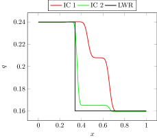
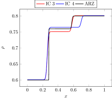
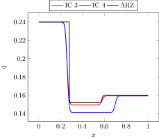
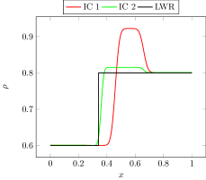
As a first example, we consider a Riemann problem for the hyperbolic equations without relaxation term. We choose N=10𝑁10N=10 and 4 different kinetic initial conditions. They are always chosen such that for x12𝑥12x\leq\frac{1}{2} we have ρ=ρL=0.6𝜌subscript𝜌𝐿0.6\rho=\rho_{L}=0.6 and for x>12𝑥12x>\frac{1}{2} we have ρ=ρR=0.8𝜌subscript𝜌𝑅0.8\rho=\rho_{R}=0.8. In all cases qLsubscript𝑞𝐿q_{L} and qRsubscript𝑞𝑅q_{R} are given by q=F(ρ)𝑞𝐹𝜌q=F(\rho) with F=ρ(1ρ)𝐹𝜌1𝜌F=\rho(1-\rho).

The first kinetic initial condition is obtained using the left and right initial distributions fL=αLδ0.4+βLδ0subscript𝑓𝐿subscript𝛼𝐿subscript𝛿0.4subscript𝛽𝐿subscript𝛿0f_{L}=\alpha_{L}\delta_{0.4}+\beta_{L}\delta_{0} and fR=αRδ0.4+βRδ0.2subscript𝑓𝑅subscript𝛼𝑅subscript𝛿0.4subscript𝛽𝑅subscript𝛿0.2f_{R}=\alpha_{R}\delta_{0.4}+\beta_{R}\delta_{0.2}, where αL/Rsubscript𝛼𝐿𝑅\alpha_{L/R} and βL/Rsubscript𝛽𝐿𝑅\beta_{L/R} are chosen such that the above macroscopic initial values are obtained. The second initial condition is given by using the same fLsubscript𝑓𝐿f_{L} and changing the values for fRsubscript𝑓𝑅f_{R} into fR=αRδ0.4+βRδ0.1subscript𝑓𝑅subscript𝛼𝑅subscript𝛿0.4subscript𝛽𝑅subscript𝛿0.1f_{R}=\alpha_{R}\delta_{0.4}+\beta_{R}\delta_{0.1} The third condition uses fL/R=αL/Rδ0.2+βL/Rδ0subscript𝑓𝐿𝑅subscript𝛼𝐿𝑅subscript𝛿0.2subscript𝛽𝐿𝑅subscript𝛿0f_{L/R}=\alpha_{L/R}\delta_{0.2}+\beta_{L/R}\delta_{0} and the fourth one fL/R=αL/Rδ0.4+βL/Rδ0subscript𝑓𝐿𝑅subscript𝛼𝐿𝑅subscript𝛿0.4subscript𝛽𝐿𝑅subscript𝛿0f_{L/R}=\alpha_{L/R}\delta_{0.4}+\beta_{L/R}\delta_{0} .

Figure 1 top row shows the solutions of the Riemann problems at t=0.4𝑡0.4t=0.4 for initial states 1 and 2 and the solution of the LWR equations with flux function ρ(1ρ)𝜌1𝜌\rho(1-\rho). Figure 1 bottom row shows the solutions of the Riemann problems for initial states 3 and4 4 and the solution of the ARZ equations tρ+x(ρu)=0subscript𝑡𝜌subscript𝑥𝜌𝑢0\partial_{t}\rho+\partial_{x}(\rho u)=0, tu+uxu+ρp(ρ)xu=0subscript𝑡𝑢𝑢subscript𝑥𝑢𝜌superscript𝑝𝜌subscript𝑥𝑢0\partial_{t}u+u\partial_{x}u+\rho p^{\prime}(\rho)\partial_{x}u=0 without right hand side and pressure p𝑝p given by p(ρ)=ρ1ρ𝑝𝜌𝜌1𝜌p(\rho)=\frac{\rho}{1-\rho}.

One observes in these figures a variety of solutions for the same ρ𝜌\rho and q𝑞q initial values depending on the kinetic initial conditions.
Refer to caption Refer to caption

Refer to caption Refer to caption

Figure 1: Density ρ𝜌\rho and flux q𝑞q for Riemann problems with ρL=0.6,ρR=0.8formulae-sequencesubscript𝜌𝐿0.6subscript𝜌𝑅0.8\rho_{L}=0.6,\rho_{R}=0.8, q=ρ(1ρ)𝑞𝜌1𝜌q=\rho(1-\rho) and 4 different kinetic initial situations. For comparison LWR and ARZ solutions are shown respectively.

7.4 Test-case 2: Decay to equilibrium for stable situation

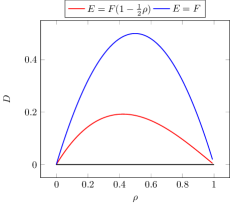
We reconsider Example 3 and the full relaxation model with ϵ=0.01italic-ϵ0.01\epsilon=0.01. As a stable example, consider E=F(ρ)(1αρ)𝐸𝐹𝜌1𝛼𝜌E=F(\rho)(1-\alpha\rho). Then, the stability condition is

(F(ρ))2+E(ρ)+11ρ[E(ρ)(F+E)(ρ)F(ρ)+F(ρ)E(ρ)]=(1F)(F+F1ρ)α(Fρ+F+F1ρ[ρ+F)])0.\displaystyle\begin{aligned} -&(F^{\prime}(\rho))^{2}+E^{\prime}(\rho)+\frac{1}{1-\rho}\left[E(\rho)-(F+E)(\rho)F^{\prime}(\rho)+F(\rho)E^{\prime}(\rho)\right]\\ &=(1-F^{\prime})\left(F^{\prime}+\frac{F}{1-\rho}\right)-\alpha\left(F^{\prime}\rho+F+\frac{F}{1-\rho}\left[\rho+F)\right]\right)\geq 0.\end{aligned}

Choosing the concave LWR fundamental diagram F(ρ)=ρ(1ρ)𝐹𝜌𝜌1𝜌F(\rho)=\rho(1-\rho), the above expression is 2ρ(1ρ)α(ρ(2+ρ)(1ρ))2𝜌1𝜌𝛼𝜌2𝜌1𝜌2\rho(1-\rho)-\alpha\left(\rho(2+\rho)(1-\rho)\right). This is larger than zero if

α2322+ρ.𝛼2322𝜌\displaystyle\alpha\leq\frac{2}{3}\leq\frac{2}{2+\rho}.

In case v1=12subscript𝑣112v_{1}=\frac{1}{2}, the function E=F(ρ)(1αρ)𝐸𝐹𝜌1𝛼𝜌E=F(\rho)(1-\alpha\rho) fulfils the realizability constraint (6) as long as α12𝛼12\alpha\leq\frac{1}{2}.

For the numerical experiments we consider E=F𝐸𝐹E=F and E=F(1ρ2)𝐸𝐹1𝜌2E=F(1-\frac{\rho}{2}). The initial conditions are defined as

fi(0,x)=13(0.7+0.1sin(6πx)),i=0,1,2.formulae-sequencesubscript𝑓𝑖0𝑥130.70.16𝜋𝑥𝑖012f_{i}(0,x)=\frac{1}{3}(0.7+0.1\sin(6\pi x)),\quad i=0,1,2.

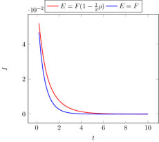
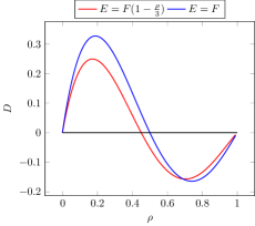
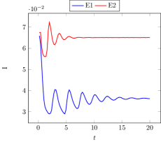
In Figure 2 the Chapman-Enskog stability term D(ρ)𝐷𝜌D(\rho) is plotted on the left. Figure 2 on the right shows a plot of the quantity

I(t)=01|ρ(x,t)0.7|𝑑x𝐼𝑡superscriptsubscript01𝜌𝑥𝑡0.7differential-d𝑥I(t)=\int_{0}^{1}|\rho(x,t)-0.7|dx

as a measure for the persistence of the periodic solution. One clearly observes that I𝐼I tends to zero in the stable cases considered here. The solution tends to the constant solution. The convergence rate is larger for larger Chapman-Enskog term D𝐷D, as expected.

Refer to caption Refer to caption

Figure 2: Decay to constant state for for N=2𝑁2N=2 with F=ρ(1ρ)𝐹𝜌1𝜌F=\rho(1-\rho) and E=F(112ρ)𝐸𝐹112𝜌E=F(1-\frac{1}{2}\rho), E=F𝐸𝐹E=F, respectively. Left: plot of stability conditions. Right: plot of decay rate I𝐼I versus time.

7.5 Test-case 3: Persistent periodic waves for unstable situations

This time we reconsider Example 4 using an equidistant spacing of the velocity points vi=iNsubscript𝑣𝑖𝑖𝑁v_{i}=\frac{i}{N} and N=20𝑁20N=20. The relaxation parameter is again chosen as ϵ=0.01italic-ϵ0.01\epsilon=0.01.

Note that in this case choosing additionally αi=2iN(N1)subscript𝛼𝑖2𝑖𝑁𝑁1\alpha_{i}=\frac{2i}{N(N-1)} one obtains

λ=i=1N1αivi=i=1N12i2N2(N1)=132N1N𝜆superscriptsubscript𝑖1𝑁1subscript𝛼𝑖subscript𝑣𝑖superscriptsubscript𝑖1𝑁12superscript𝑖2superscript𝑁2𝑁1132𝑁1𝑁\displaystyle\lambda=\sum_{i=1}^{N-1}\alpha_{i}v_{i}=\sum_{i=1}^{N-1}\frac{2i^{2}}{N^{2}(N-1)}=\frac{1}{3}\frac{2N-1}{N}

and

γ=i=1N1αivi=i=1N12iNiN(N1)=2.𝛾superscriptsubscript𝑖1𝑁1subscript𝛼𝑖subscript𝑣𝑖superscriptsubscript𝑖1𝑁12𝑖𝑁𝑖𝑁𝑁12\displaystyle\gamma=\sum_{i=1}^{N-1}\frac{\alpha_{i}}{v_{i}}=\sum_{i=1}^{N-1}\frac{2iN}{iN(N-1)}=2.

We obtain for the equilibrium functions

fie(ρ,v)superscriptsubscript𝑓𝑖𝑒𝜌𝑣\displaystyle f_{i}^{e}(\rho,v) =6N1NN+1(FE),i=1,,N1formulae-sequenceabsent6𝑁1𝑁𝑁1𝐹𝐸𝑖1𝑁1\displaystyle=\frac{6}{N-1}\frac{N}{N+1}(F-E),\quad i=1,\ldots,N-1
fNe(ρ,v)superscriptsubscript𝑓𝑁𝑒𝜌𝑣\displaystyle f_{N}^{e}(\rho,v) =F3NN+1(FE)absent𝐹3𝑁𝑁1𝐹𝐸\displaystyle=F-3\frac{N}{N+1}(F-E)
f0e(ρ,v)superscriptsubscript𝑓0𝑒𝜌𝑣\displaystyle f_{0}^{e}(\rho,v) =ρF3N1N+1(FE).absent𝜌𝐹3𝑁1𝑁1𝐹𝐸\displaystyle=\rho-F-3\frac{N-1}{N+1}(F-E).

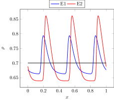
To obtain an unstable situation we choose here the non-concave function F=ρ(1ρ)2𝐹𝜌superscript1𝜌2F=\rho(1-\rho)^{2} and E=F(113ρ)𝐸𝐹113𝜌E=F(1-\frac{1}{3}\rho) and E=F𝐸𝐹E=F, respectively. The functions E𝐸E fulfil the realizability condition (3). We consider the periodic initial condition

fi(0,x)=1N+1(0.7+0.1sin(6πx)),i=0,,N.formulae-sequencesubscript𝑓𝑖0𝑥1𝑁10.70.16𝜋𝑥𝑖0𝑁f_{i}(0,x)=\frac{1}{N+1}(0.7+0.1\sin(6\pi x)),\quad i=0,\ldots,N.

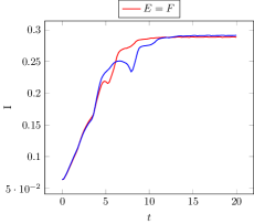
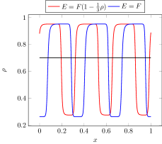
In Figure 3 on the left, the functions F𝐹F and E=F(113ρ)𝐸𝐹113𝜌E=F(1-\frac{1}{3}\rho) and the lower bound of the realizability domain are plotted. On the right the Chapman -Enskog stability term D(ρ)𝐷𝜌D(\rho) is plotted.

Figure 4 shows on the left a plot of I𝐼I defined as above. One observes that I𝐼I tends to a positive value for the unstable cases considered in this subsection. On the right, the density ρ𝜌\rho is plotted at the final time T=20𝑇20T=20 showing the persistent periodic solutions for the two unstable cases considered here.
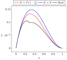
Refer to caption Refer to caption


Figure 3: Persistence of waves in unstable situations, N=20𝑁20N=20. Left: functions F=ρ(1ρ)2𝐹𝜌superscript1𝜌2F=\rho(1-\rho)^{2} and E=F(113ρ)𝐸𝐹113𝜌E=F(1-\frac{1}{3}\rho) and realizability region. Right: stability conditions for E=F(113ρ)𝐸𝐹113𝜌E=F(1-\frac{1}{3}\rho) and E=F𝐸𝐹E=F.

Refer to caption Refer to caption

Figure 4: Persistence of waves in unstable situation with F=ρ(1ρ)2𝐹𝜌superscript1𝜌2F=\rho(1-\rho)^{2} and E=F(113ρ)𝐸𝐹113𝜌E=F(1-\frac{1}{3}\rho), E=F𝐸𝐹E=F, respectively. Left: plot of I𝐼I versus time. Right: plot of ρ𝜌\rho at final time T=20𝑇20T=20 for N=20𝑁20N=20.

7.6 Test-case 4: Persistent periodic waves for a weakly unstable situation

We consider again Example 3 with N=2𝑁2N=2. As in the first example we consider the concave flux function F(ρ)=ρ(1ρ)𝐹𝜌𝜌1𝜌F(\rho)=\rho(1-\rho). Here we obtain unstable situations by choosing appropriate E𝐸E leading to non-positive D(ρ)𝐷𝜌D(\rho). Thus, the relation beween flux and variance of the equilibrium distribution plays a major role in the appearance of persistent waves.

We consider two numerical choices for the function E𝐸E. In both cases, E𝐸E is for smaller values of ρ𝜌\rho given by the flux function F𝐹F. For larger values of ρ𝜌\rho near 111 we have chosen E1subscript𝐸1E_{1} to be given by E1=14(ρ1)(ρ3)subscript𝐸114𝜌1𝜌3E_{1}=\frac{1}{4}(\rho-1)(\rho-3) and E2subscript𝐸2E_{2} by the lower boundary of the realizability domain. In between a 𝒞2superscript𝒞2\mathcal{C}^{2}-spline interpolation is used for both cases.

In Figure 5 on the left the functions F,E1𝐹subscript𝐸1F,E_{1} and E2subscript𝐸2E_{2} and the realizability domain for v1=12subscript𝑣112v_{1}=\frac{1}{2} are plotted. On the right the Chapman -Enskog stability terms are plotted for the two choices of E𝐸E.

The initial conditions are again

fi(0,x)=13(0.7+0.1sin(6πx)),i=0,1,2.formulae-sequencesubscript𝑓𝑖0𝑥130.70.16𝜋𝑥𝑖012f_{i}(0,x)=\frac{1}{3}(0.7+0.1\sin(6\pi x)),\quad i=0,1,2.

Figure 6 shows on the left a plot of

I(t)=01|ρ(x,t)0.7|𝑑x𝐼𝑡superscriptsubscript01𝜌𝑥𝑡0.7differential-d𝑥I(t)=\int_{0}^{1}|\rho(x,t)-0.7|dx

as a measure for the persistence of the periodic solution. One observes that I𝐼I tends positive values for the unstable cases. On the right the density ρ𝜌\rho is plotted at the final time T=20𝑇20T=20 for the unstable situations. Note that the values og I𝐼I for large t𝑡t are smaller than the corresponding values in the previous example. The persistent waves are, correspondingly, less pronounced.
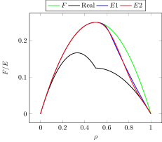
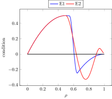
Refer to caption Refer to caption

Figure 5: Persistence of waves in unstable situations, N=2𝑁2N=2. Left: functions F𝐹F, E1subscript𝐸1E_{1} and E2subscript𝐸2E_{2} and realizability region. Right: stability conditions for E1subscript𝐸1E_{1} and E2subscript𝐸2E_{2}.

Refer to caption Refer to caption

Figure 6: Persistence of waves in unstable situations. Left: Plot of I𝐼I versus time for E1subscript𝐸1E_{1} and E2subscript𝐸2E_{2}. Right: plot of the density ρ𝜌\rho for the final time T=20𝑇20T=20 for N=2𝑁2N=2.

8 Conclusions and outlook

The paper presents a new class of non-linear kinetic discrete velocity models for traffic flow having the correct invariant domain for traffic flow modelling and allowing for negative wave-speeds despite the positivity of the microscopic velocities. The hyperbolic part is non-linear, but relatively simple, being a totally linear degenerate and rich hyperbolic problem with a simple structure of the integral curves. For the homogeneous system, the fact, that the hyperbolic system is rich and totally linear degenerate, yields existence of global entropy solutions, see [35, 25]. For the relaxation system the so-called semi-linear behaviour is obtained in [9] preventing the appearance of shock solutions. Moreover, we have investigated conditions on the flux function F𝐹F such that stop-and-go-wave like instabilities arise, similar to investigations that has been performed for the Aw-Rascle model in [16]. Numerical results illustrate the behaviour of the solutions of Riemann problems wiout relaxation term and the persistence of periodic solutions for the full relaxation problem for various situations. In particular, it turns out that the relation between flux and variance of the equilibrium distribution plays a major role in the appearance of persistent waves. Further research will be concerned with the development of higher order numerical methods for the kinetic equations and a closer investigation of the persistent periodic waves appearing for the relaxation problem.

References

  • [1] A. Aw and M. Rascle, Resurrection of second order models of traffic flow?, SIAM J. Appl. Math., 60, 916–938, 2000.
  • [2] A. Aw, A. Klar, T. Materne, M. Rascle, Derivation of continuum flow traffic models from microscopic Follow the leader models, SIAM J. Appl. Math. 63 (1), 259-278, 2002
  • [3] N. Bellomo, C. Dogbe, On the Modeling of Traffic and Crowds: A Survey of Models, Speculations, and Perspectives, SIAM Review 53, 3, 409-463, 2011.
  • [4] F. Berthelin, P. Degond, V. Le Blanc, S. Moutari, J. Royer, M. Rascle, A Traffic-Flow Model with Constraints for the Modeling of Traffic Jams, Mathematical Models and Methods in Applied Sciences 18, 1269-1298, 2008
  • [5] F. Berthelin, P. Degond, M. Delitala, M. Rascle, A model for the formation and evolution of traffic jams Arch. Rat. Mech. Anal. 187, 185-220, 2008.
  • [6] R. Borsche, A. Klar, A nonlinear discrete-velocity relaxation model for traffic flow, SIAM J. Applied Mathematics, 78 (5), 2891-2917, 2018
  • [7] R. Borsche, A. Klar and M. Zanella, Kinetic-controlled hydrodynamics for multilane traffic models, Phys. A, 587, 126486, 2022.
  • [8] R. Borsche, M. Kimathi, A. Klar, Kinetic derivations of a Hamilton-Jacobi type traffic flow model, Comm. Math. Sci., 11,3, 739-756, 2013
  • [9] G. Carbou, B. Hanouzet, R. Natalini, Semilinear behavior for totally linearly degenerate hyperbolic systems with relaxation, J. Differential Equations 246, 291–319, 2009
  • [10] F.A. Chiarello, A. Tosin, Macroscopic limits of non-local kinetic descriptions of vehicular traffic, Kinetic and Related Models, 1937-5093), 2022
  • [11] G. Dimarco and A. Tosin, The Aw-Rascle traffic model: Enskog-type kinetic derivation and generalisations, J. Stat. Phys., 178, 2020.
  • [12] G. Dimarco, A. Tosin and M. Zanella, Kinetic derivation of Aw–Rascle–Zhang-type traffic models with driver-assist vehicles, J. Stat. Phys., 186, 2022
  • [13] M. R. Flynn, A. R. Kasimov, J.-C. Nave, R. R. Rosales, B. Seibold, Self-sustained nonlinear waves in traffic flow Phys. Rev. E, Vol. 79, 5, 056113, 2009
  • [14] L. Fermo and A. Tosin, A fully-discrete-state kinetic theory approach to modeling vehicular traffic, SIAM Journal on Applied Mathematics 73 (4), 1533-1556, 2013
  • [15] J.M. Greenberg, Extension and amplification of the Aw-Rascle model, SIAM J. Appl. Math., 62 (2001), pp. 729–745.
  • [16] J.M. Greenberg, Congestion redux, SIAM J. Appl. Math, 64 (2004), 1175–1185, 2004
  • [17] J.M. Greenberg, A. Klar, and M. Rascle, Congestion on multilane highways, SIAM J. Appl. Math, 63, 818-833, 2003.
  • [18] D. Helbing, Gas-kinetic derivation of Navier-Stokes-like traffic equation, Physical Review E, 53 (1996), pp. 2366–2381.
  • [19] M. Herty and G. Puppo and S. Roncoroni and G. Visconti, The BGK approximation of kinetic models for traffic, Kinetic & Related Models 13, 2, 279-307, 2020.
  • [20] R. Illner, T. Platkowski,Discrete Velocity Models of the Boltzmann Equation: A Survey on the Mathematical ASPECTS of the Theory, SIAM Rev., 30(2), 213-255, 1988.
  • [21] A. Klar and R. Wegener, Enskog-like kinetic models for vehicular traffic, J. Stat. Phys., 87 , 91-114, 1997.
  • [22] A. Klar and R. Wegener, A hierachy of models for multilane vehicular traffic I: Modeling, SIAM J. Appl. Math., 59, 983-1001, 1998.
  • [23] A. Klar and R. Wegener, Kinetic derivation of macroscopic anticipation models for vehicular traffic, SIAM J. Appl. Math., 60 , 1749-1766, 2000.
  • [24] M. Lachowicz, On the hydrodynamic limit of the Enskog equation, Publ. RIMS, Kyoto Univ. 34, 191-210, 1998
  • [25] T.T. Li and Y.J. Peng and J. Ruiz, Entropy solutions for linearly degenerate hyperbolic systems of rich type, Journal de Mathématiques Pures et Appliquées 91, 6, 553-568, 2009.
  • [26] T.P. Liu, Hyperbolic conservation laws with relaxation, Communications in Mathematical Physics 108, 1, 153–175, 1987
  • [27] P. Nelson, A kinetic model of vehicular traffic and its associated bimodal equilibrium solutions, Transport Theory and Statistical Physics, 24 (1995), pp. 383–408.
  • [28] L. Pareschi and G. Russo, Implicit-Explicit Runge-Kutta Schemes and Applications to Hyperbolic Systems with Relaxation, Journal of Scientific Computing, 25, 1/2, 2005
  • [29] S. Paveri-Fontana, On Boltzmann like treatments for traffic flow, Transportation Research, 9 (1975), pp. 225–235.
  • [30] Payne, H.J. Models of freeway traffic and control. In Mathematical Models of Public Systems; Simulation Council: Raleigh, NC, USA, 1971; Volume 1, pp. 51–61.
  • [31] Y.-J. Peng, Entropy solutions for linearly degenerate hyperbolic systems of rich type, Journal de Mathématiques Pures et Appliqués, 2009
  • [32] D. Serre, Richness and the classification of quasilinear hyperbolic systems. Multidimen- sional hyperbolic problems and computations (Minneapolis, 1989), 315-333, IMA Vol. Math. Appl. 29, Springer, New York, 1991.
  • [33] I. Prigogine and R. Herman, Kinetic Theory of Vehicular Traffic, American Elsevier Publishing Co., New York, 1971.
  • [34] M. Rascle, An Improved Macroscopic Model of Traffic Flow: Derivation and Links with the Lighthill-Whitham Model, Mathematical and Computer Modelling 35, 581-590, 2002.
  • [35] B.L. Rozhdestvenskii, A.D. Sidorenko, Impossibility of the gradient catastrophe for slightly non-linear systems, Zh. Vychisl. Mat. Mat. Fiz. 7 1176–1179, 1967.
  • [36] G. Whitham, Linear and Nonlinear Waves, Wiley, New York, 1974.
  • [37] H. M. Zhang, A non-equilibrium traffic model devoid of gas-like behavior, Transp. Research B, 36, 3, 275-290, 2002

9 Appendix

Consider for k=0,,N1𝑘0𝑁1k=0,\ldots,N-1 the eigenvalues

λk(w)subscript𝜆𝑘𝑤\displaystyle\lambda_{k}(w) =vk(vk+1vk)wk+1+j=k+2N(vjvk)wjl=k+1j1(1wl)j=k+1N(1wj).absentsubscript𝑣𝑘subscript𝑣𝑘1subscript𝑣𝑘subscript𝑤𝑘1superscriptsubscript𝑗𝑘2𝑁subscript𝑣𝑗subscript𝑣𝑘subscript𝑤𝑗superscriptsubscriptproduct𝑙𝑘1𝑗11subscript𝑤𝑙superscriptsubscriptproduct𝑗𝑘1𝑁1subscript𝑤𝑗\displaystyle=v_{k}-\frac{(v_{k+1}-v_{k})w_{k+1}+\sum_{j=k+2}^{N}(v_{j}-v_{k})w_{j}\prod_{l=k+1}^{j-1}(1-w_{l})}{\prod_{j=k+1}^{N}(1-w_{j})}.

For j>k𝑗𝑘j>k we prove (8), i.e.

λk(w)wj=λjλk1wj.subscript𝜆𝑘𝑤subscript𝑤𝑗subscript𝜆𝑗subscript𝜆𝑘1subscript𝑤𝑗\displaystyle\frac{\partial\lambda_{k}(w)}{\partial w_{j}}=-\frac{\lambda_{j}-\lambda_{k}}{1-w_{j}}.

Consider first the case j=k+1𝑗𝑘1j=k+1, then

λk(w)wk+1subscript𝜆𝑘𝑤subscript𝑤𝑘1\displaystyle\frac{\partial\lambda_{k}(w)}{\partial w_{k+1}} =wk+1((vk+1vk)wk+1+j=k+2N(vjvk)wjl=k+1j1(1wl)j=k+1N(1wj))absentsubscript𝑤𝑘1subscript𝑣𝑘1subscript𝑣𝑘subscript𝑤𝑘1superscriptsubscript𝑗𝑘2𝑁subscript𝑣𝑗subscript𝑣𝑘subscript𝑤𝑗superscriptsubscriptproduct𝑙𝑘1𝑗11subscript𝑤𝑙superscriptsubscriptproduct𝑗𝑘1𝑁1subscript𝑤𝑗\displaystyle=-\frac{\partial}{\partial w_{k+1}}\left(\frac{(v_{k+1}-v_{k})w_{k+1}+\sum_{j=k+2}^{N}(v_{j}-v_{k})w_{j}\prod_{l=k+1}^{j-1}(1-w_{l})}{\prod_{j=k+1}^{N}(1-w_{j})}\right)
=(vk+1vk)j=k+1N(1wj)+(vk+1vk)wk+1j=k+2N(1wj)(j=k+1N(1wj))2absentsubscript𝑣𝑘1subscript𝑣𝑘superscriptsubscriptproduct𝑗𝑘1𝑁1subscript𝑤𝑗subscript𝑣𝑘1subscript𝑣𝑘subscript𝑤𝑘1superscriptsubscriptproduct𝑗𝑘2𝑁1subscript𝑤𝑗superscriptsuperscriptsubscriptproduct𝑗𝑘1𝑁1subscript𝑤𝑗2\displaystyle=-\frac{(v_{k+1}-v_{k})\prod_{j=k+1}^{N}(1-w_{j})+(v_{k+1}-v_{k})w_{k+1}\prod_{j=k+2}^{N}(1-w_{j})}{(\prod_{j=k+1}^{N}(1-w_{j}))^{2}}
=(vk+1vk)(1wk+1)+(vk+1vk)wk+1(1wk+1)2j=k+2N(1wj)absentsubscript𝑣𝑘1subscript𝑣𝑘1subscript𝑤𝑘1subscript𝑣𝑘1subscript𝑣𝑘subscript𝑤𝑘1superscript1subscript𝑤𝑘12superscriptsubscriptproduct𝑗𝑘2𝑁1subscript𝑤𝑗\displaystyle=-\frac{(v_{k+1}-v_{k})(1-w_{k+1})+(v_{k+1}-v_{k})w_{k+1}}{(1-w_{k+1})^{2}\prod_{j=k+2}^{N}(1-w_{j})}
=vk+1vk(1wk+1)j=k+1N(1wj)absentsubscript𝑣𝑘1subscript𝑣𝑘1subscript𝑤𝑘1superscriptsubscriptproduct𝑗𝑘1𝑁1subscript𝑤𝑗\displaystyle=-\frac{v_{k+1}-v_{k}}{(1-w_{k+1})\prod_{j=k+1}^{N}(1-w_{j})}
=vk+1vk1wk+11j=0kfj1ρ,absentsubscript𝑣𝑘1subscript𝑣𝑘1subscript𝑤𝑘11superscriptsubscript𝑗0𝑘subscript𝑓𝑗1𝜌\displaystyle=-\frac{v_{k+1}-v_{k}}{1-w_{k+1}}\frac{1-\sum_{j=0}^{k}f_{j}}{1-\rho},

since

1j=0kfj=1w0j=1kwjl=0i1(1wl)1superscriptsubscript𝑗0𝑘subscript𝑓𝑗1subscript𝑤0superscriptsubscript𝑗1𝑘subscript𝑤𝑗superscriptsubscriptproduct𝑙0𝑖11subscript𝑤𝑙\displaystyle 1-\sum_{j=0}^{k}f_{j}=1-w_{0}-\sum_{j=1}^{k}w_{j}\prod_{l=0}^{i-1}(1-w_{l})
=(1w0)(1w1j=2kwjl=1i1(1wl))==j=0k(1wj).absent1subscript𝑤01subscript𝑤1superscriptsubscript𝑗2𝑘subscript𝑤𝑗superscriptsubscriptproduct𝑙1𝑖11subscript𝑤𝑙superscriptsubscriptproduct𝑗0𝑘1subscript𝑤𝑗\displaystyle=(1-w_{0})(1-w_{1}-\sum_{j=2}^{k}w_{j}\prod_{l=1}^{i-1}(1-w_{l}))=\cdots=\prod_{j=0}^{k}(1-w_{j}).

In the general case, we compute for j>k+1𝑗𝑘1j>k+1

λk(w)wjsubscript𝜆𝑘𝑤subscript𝑤𝑗\displaystyle\frac{\partial\lambda_{k}(w)}{\partial w_{j}} =wj((vk+1vk)wk+1+l=k+2N(vlvk)wlr=k+1l1(1wr)l=k+1N(1wl))absentsubscript𝑤𝑗subscript𝑣𝑘1subscript𝑣𝑘subscript𝑤𝑘1superscriptsubscript𝑙𝑘2𝑁subscript𝑣𝑙subscript𝑣𝑘subscript𝑤𝑙superscriptsubscriptproduct𝑟𝑘1𝑙11subscript𝑤𝑟superscriptsubscriptproduct𝑙𝑘1𝑁1subscript𝑤𝑙\displaystyle=-\frac{\partial}{\partial w_{j}}\left(\frac{(v_{k+1}-v_{k})w_{k+1}+\sum_{l=k+2}^{N}(v_{l}-v_{k})w_{l}\prod_{r=k+1}^{l-1}(1-w_{r})}{\prod_{l=k+1}^{N}(1-w_{l})}\right)
=(vjvk)r=k+1j1(1wr)11wjl=j+1N(vlvk)wlr=k+1l1(1wr)l=k+1N(1wl)absentsubscript𝑣𝑗subscript𝑣𝑘superscriptsubscriptproduct𝑟𝑘1𝑗11subscript𝑤𝑟11subscript𝑤𝑗superscriptsubscript𝑙𝑗1𝑁subscript𝑣𝑙subscript𝑣𝑘subscript𝑤𝑙superscriptsubscriptproduct𝑟𝑘1𝑙11subscript𝑤𝑟superscriptsubscriptproduct𝑙𝑘1𝑁1subscript𝑤𝑙\displaystyle=-\frac{(v_{j}-v_{k})\prod_{r=k+1}^{j-1}(1-w_{r})-\frac{1}{1-w_{j}}\sum_{l=j+1}^{N}(v_{l}-v_{k})w_{l}\prod_{r=k+1}^{l-1}(1-w_{r})}{\prod_{l=k+1}^{N}(1-w_{l})}
11wj(vk+1vk)wk+1+l=k+2N(vlvk)wlr=k+1l1(1wr)l=k+1N(1wl)11subscript𝑤𝑗subscript𝑣𝑘1subscript𝑣𝑘subscript𝑤𝑘1superscriptsubscript𝑙𝑘2𝑁subscript𝑣𝑙subscript𝑣𝑘subscript𝑤𝑙superscriptsubscriptproduct𝑟𝑘1𝑙11subscript𝑤𝑟superscriptsubscriptproduct𝑙𝑘1𝑁1subscript𝑤𝑙\displaystyle-\frac{1}{1-w_{j}}\frac{(v_{k+1}-v_{k})w_{k+1}+\sum_{l=k+2}^{N}(v_{l}-v_{k})w_{l}\prod_{r=k+1}^{l-1}(1-w_{r})}{\prod_{l=k+1}^{N}(1-w_{l})}

This yields

λk(w)wjsubscript𝜆𝑘𝑤subscript𝑤𝑗\displaystyle\frac{\partial\lambda_{k}(w)}{\partial w_{j}} =(vjvk)r=k+1j1(1wr)l=k+1N(1wl)11wj(vk+1vk)wk+1l=k+1N(1wl)absentsubscript𝑣𝑗subscript𝑣𝑘superscriptsubscriptproduct𝑟𝑘1𝑗11subscript𝑤𝑟superscriptsubscriptproduct𝑙𝑘1𝑁1subscript𝑤𝑙11subscript𝑤𝑗subscript𝑣𝑘1subscript𝑣𝑘subscript𝑤𝑘1superscriptsubscriptproduct𝑙𝑘1𝑁1subscript𝑤𝑙\displaystyle=-\frac{(v_{j}-v_{k})\prod_{r=k+1}^{j-1}(1-w_{r})}{\prod_{l=k+1}^{N}(1-w_{l})}-\frac{1}{1-w_{j}}\frac{(v_{k+1}-v_{k})w_{k+1}}{\prod_{l=k+1}^{N}(1-w_{l})}
+11wjl=j+1N(vlvk)wlr=k+1l1(1wr)l=k+1N(1wl)11subscript𝑤𝑗superscriptsubscript𝑙𝑗1𝑁subscript𝑣𝑙subscript𝑣𝑘subscript𝑤𝑙superscriptsubscriptproduct𝑟𝑘1𝑙11subscript𝑤𝑟superscriptsubscriptproduct𝑙𝑘1𝑁1subscript𝑤𝑙\displaystyle+\frac{\frac{1}{1-w_{j}}\sum_{l=j+1}^{N}(v_{l}-v_{k})w_{l}\prod_{r=k+1}^{l-1}(1-w_{r})}{\prod_{l=k+1}^{N}(1-w_{l})}
11wjl=k+2N(vlvk)wlr=k+1l1(1wr)l=k+1N(1wl)11subscript𝑤𝑗superscriptsubscript𝑙𝑘2𝑁subscript𝑣𝑙subscript𝑣𝑘subscript𝑤𝑙superscriptsubscriptproduct𝑟𝑘1𝑙11subscript𝑤𝑟superscriptsubscriptproduct𝑙𝑘1𝑁1subscript𝑤𝑙\displaystyle-\frac{1}{1-w_{j}}\frac{\sum_{l=k+2}^{N}(v_{l}-v_{k})w_{l}\prod_{r=k+1}^{l-1}(1-w_{r})}{\prod_{l=k+1}^{N}(1-w_{l})}
=(vjvk)r=k+1j1(1wr)l=k+1N(1wl)11wj(vk+1vk)wk+1l=k+1N(1wl)absentsubscript𝑣𝑗subscript𝑣𝑘superscriptsubscriptproduct𝑟𝑘1𝑗11subscript𝑤𝑟superscriptsubscriptproduct𝑙𝑘1𝑁1subscript𝑤𝑙11subscript𝑤𝑗subscript𝑣𝑘1subscript𝑣𝑘subscript𝑤𝑘1superscriptsubscriptproduct𝑙𝑘1𝑁1subscript𝑤𝑙\displaystyle=-\frac{(v_{j}-v_{k})\prod_{r=k+1}^{j-1}(1-w_{r})}{\prod_{l=k+1}^{N}(1-w_{l})}-\frac{1}{1-w_{j}}\frac{(v_{k+1}-v_{k})w_{k+1}}{\prod_{l=k+1}^{N}(1-w_{l})}
11wjl=k+2j(vlvk)wlr=k+1l1(1wr)l=k+1N(1wl)11subscript𝑤𝑗superscriptsubscript𝑙𝑘2𝑗subscript𝑣𝑙subscript𝑣𝑘subscript𝑤𝑙superscriptsubscriptproduct𝑟𝑘1𝑙11subscript𝑤𝑟superscriptsubscriptproduct𝑙𝑘1𝑁1subscript𝑤𝑙\displaystyle-\frac{1}{1-w_{j}}\frac{\sum_{l=k+2}^{j}(v_{l}-v_{k})w_{l}\prod_{r=k+1}^{l-1}(1-w_{r})}{\prod_{l=k+1}^{N}(1-w_{l})}

and then

λk(w)wjsubscript𝜆𝑘𝑤subscript𝑤𝑗\displaystyle\frac{\partial\lambda_{k}(w)}{\partial w_{j}} =11wj(vjvk)r=k+1j(1wr)l=k+1N(1wl)11wj(vk+1vk)wk+1l=k+1N(1wl)absent11subscript𝑤𝑗subscript𝑣𝑗subscript𝑣𝑘superscriptsubscriptproduct𝑟𝑘1𝑗1subscript𝑤𝑟superscriptsubscriptproduct𝑙𝑘1𝑁1subscript𝑤𝑙11subscript𝑤𝑗subscript𝑣𝑘1subscript𝑣𝑘subscript𝑤𝑘1superscriptsubscriptproduct𝑙𝑘1𝑁1subscript𝑤𝑙\displaystyle=-\frac{1}{1-w_{j}}\frac{(v_{j}-v_{k})\prod_{r=k+1}^{j}(1-w_{r})}{\prod_{l=k+1}^{N}(1-w_{l})}-\frac{1}{1-w_{j}}\frac{(v_{k+1}-v_{k})w_{k+1}}{\prod_{l=k+1}^{N}(1-w_{l})}
11wjl=k+2j(vlvk)wlr=k+1l1(1wr)l=k+1N(1wl)11subscript𝑤𝑗superscriptsubscript𝑙𝑘2𝑗subscript𝑣𝑙subscript𝑣𝑘subscript𝑤𝑙superscriptsubscriptproduct𝑟𝑘1𝑙11subscript𝑤𝑟superscriptsubscriptproduct𝑙𝑘1𝑁1subscript𝑤𝑙\displaystyle-\frac{1}{1-w_{j}}\frac{\sum_{l=k+2}^{j}(v_{l}-v_{k})w_{l}\prod_{r=k+1}^{l-1}(1-w_{r})}{\prod_{l=k+1}^{N}(1-w_{l})}
=11wj((vjvk)1r=j+1N(1wr)+l=k+1j(vlvk)wl1r=lN(1wr))absent11subscript𝑤𝑗subscript𝑣𝑗subscript𝑣𝑘1superscriptsubscriptproduct𝑟𝑗1𝑁1subscript𝑤𝑟superscriptsubscript𝑙𝑘1𝑗subscript𝑣𝑙subscript𝑣𝑘subscript𝑤𝑙1superscriptsubscriptproduct𝑟𝑙𝑁1subscript𝑤𝑟\displaystyle=-\frac{1}{1-w_{j}}\left((v_{j}-v_{k})\frac{1}{\prod_{r=j+1}^{N}(1-w_{r})}+\sum_{l=k+1}^{j}(v_{l}-v_{k})w_{l}\frac{1}{\prod_{r=l}^{N}(1-w_{r})}\right)
=11wj((vjvk)l=0j(1wl)r=0N(1wr)l=k+1j(vlvk)wlr=0l1(1wr)r=0N(1wr))absent11subscript𝑤𝑗subscript𝑣𝑗subscript𝑣𝑘superscriptsubscriptproduct𝑙0𝑗1subscript𝑤𝑙superscriptsubscriptproduct𝑟0𝑁1subscript𝑤𝑟superscriptsubscript𝑙𝑘1𝑗subscript𝑣𝑙subscript𝑣𝑘subscript𝑤𝑙superscriptsubscriptproduct𝑟0𝑙11subscript𝑤𝑟superscriptsubscriptproduct𝑟0𝑁1subscript𝑤𝑟\displaystyle=-\frac{1}{1-w_{j}}\left((v_{j}-v_{k})\frac{\prod_{l=0}^{j}(1-w_{l})}{\prod_{r=0}^{N}(1-w_{r})}-\frac{\sum_{l=k+1}^{j}(v_{l}-v_{k})w_{l}\prod_{r=0}^{l-1}(1-w_{r})}{\prod_{r=0}^{N}(1-w_{r})}\right)
=11wj((vjvk)1l=0jfl1ρ+l=k+1j(vlvk)fl1ρ).absent11subscript𝑤𝑗subscript𝑣𝑗subscript𝑣𝑘1superscriptsubscript𝑙0𝑗subscript𝑓𝑙1𝜌superscriptsubscript𝑙𝑘1𝑗subscript𝑣𝑙subscript𝑣𝑘subscript𝑓𝑙1𝜌\displaystyle=-\frac{1}{1-w_{j}}\left((v_{j}-v_{k})\frac{1-\sum_{l=0}^{j}f_{l}}{1-\rho}+\frac{\sum_{l=k+1}^{j}(v_{l}-v_{k})f_{l}}{1-\rho}\right).

On the other hand we have for j>k𝑗𝑘j>k

λj(w)λk(w)subscript𝜆𝑗𝑤subscript𝜆𝑘𝑤\displaystyle\lambda_{j}(w)-\lambda_{k}(w)
=vjvk11ρ(l=j+1N(vlvj)fll=k+1N(vlvk)fl)absentsubscript𝑣𝑗subscript𝑣𝑘11𝜌superscriptsubscript𝑙𝑗1𝑁subscript𝑣𝑙subscript𝑣𝑗subscript𝑓𝑙superscriptsubscript𝑙𝑘1𝑁subscript𝑣𝑙subscript𝑣𝑘subscript𝑓𝑙\displaystyle=v_{j}-v_{k}-\frac{1}{1-\rho}\left(\sum_{l=j+1}^{N}(v_{l}-v_{j})f_{l}-\sum_{l=k+1}^{N}(v_{l}-v_{k})f_{l}\right)
=vjvk11ρ(l=j+1N(vkvj)fll=k+1j(vlvk)fl)absentsubscript𝑣𝑗subscript𝑣𝑘11𝜌superscriptsubscript𝑙𝑗1𝑁subscript𝑣𝑘subscript𝑣𝑗subscript𝑓𝑙superscriptsubscript𝑙𝑘1𝑗subscript𝑣𝑙subscript𝑣𝑘subscript𝑓𝑙\displaystyle=v_{j}-v_{k}-\frac{1}{1-\rho}\left(\sum_{l=j+1}^{N}(v_{k}-v_{j})f_{l}-\sum_{l=k+1}^{j}(v_{l}-v_{k})f_{l}\right)
=(vjvk)(1+11ρl=j+1Nfl)+11ρl=k+1j(vlvk)flabsentsubscript𝑣𝑗subscript𝑣𝑘111𝜌superscriptsubscript𝑙𝑗1𝑁subscript𝑓𝑙11𝜌superscriptsubscript𝑙𝑘1𝑗subscript𝑣𝑙subscript𝑣𝑘subscript𝑓𝑙\displaystyle=(v_{j}-v_{k})\left(1+\frac{1}{1-\rho}\sum_{l=j+1}^{N}f_{l}\right)+\frac{1}{1-\rho}\sum_{l=k+1}^{j}(v_{l}-v_{k})f_{l}
=(vjvk)1l=0jfl1ρ+11ρl=k+1j(vlvk)flabsentsubscript𝑣𝑗subscript𝑣𝑘1superscriptsubscript𝑙0𝑗subscript𝑓𝑙1𝜌11𝜌superscriptsubscript𝑙𝑘1𝑗subscript𝑣𝑙subscript𝑣𝑘subscript𝑓𝑙\displaystyle=(v_{j}-v_{k})\frac{1-\sum_{l=0}^{j}f_{l}}{1-\rho}+\frac{1}{1-\rho}\sum_{l=k+1}^{j}(v_{l}-v_{k})f_{l}

Altogether we have proven (8) for j>k𝑗𝑘j>k.