Pointwise Representational Similarity

Abstract

With the increasing reliance on deep neural networks, it is important to develop ways to better understand their learned representations. Representation similarity measures have emerged as a popular tool for examining learned representations. However, existing measures only provide aggregate estimates of similarity at a global level, i.e. over a set of representations for N input examples. As such, these measures are not well-suited for investigating representations at a local level, i.e. representations of a single input example. Local similarity measures are needed, for instance, to understand which individual input representations are affected by training interventions to models (e.g. to be more fair and unbiased) or are at greater risk of being misclassified. In this work, we fill in this gap and propose Pointwise Normalized Kernel Alignment (PNKA), a measure that quantifies how similarly an individual input is represented in two representation spaces. Intuitively, PNKA compares the similarity of an input’s neighborhoods across both spaces. Using our measure, we are able to analyze properties of learned representations at a finer granularity than what was previously possible. Concretely, we show how PNKA can be leveraged to develop a deeper understanding of (a) the input examples that are likely to be misclassified, (b) the concepts encoded by (individual) neurons in a layer, and (c) the effects of fairness interventions on learned representations.

1 Introduction

The success of deep neural network (DNN) models can be attributed to their ability to learn powerful representations of data that enable them to be effective across a diverse set of applications. Many promising lines of work on improving model performance continue to focus on learning better representations, such as self-supervised learning for vision (8; 17), language modeling (12) and multimodal embeddings that captures both vision and language (38).

However, the impressive performance of these models on benchmarks is often overshadowed by a variety of reliability concerns that arise when they are deployed in real-world scenarios, such as a lack of robustness to distribution shifts (15; 20; 44) and attacks (43; 37), and discriminatory behavior against certain groups of people (43; 3; 31; 2; 36). These concerns have led to a surge in interest in better understanding the internal representations of these models before deploying them (1; 10; 24).

One promising line of recent research that offers a deeper understanding of model representations is representation similarity (23; 26; 40; 32). At their core, representation similarity measures quantify how a set of points are positioned relative to each other within the representation spaces of two different models. By enabling the comparison of representations learned by two different models, these measures allow researchers to conduct a variety of ablation studies of training DNN models.

However, existing representational similarity measures have a serious limitation that has been surprisingly overlooked by prior works: the current representation similarity measures only provide aggregate estimates of similarity at a global level of N input examples. Such overall similarity estimates do not provide the ability to investigate representation similarity at a local level for individual input examples. Such fine-grained similarity estimates are crucially important to understand whether the difference in representations of two models can be attributed to some specific subset or all of the input examples.

To enable the analysis of representation similarity in a more fine-grained manner, we propose Pointwise Normalized Kernel Alignment (PNKA), a measure that assigns similarity scores to individual data points . Our measure can be used to answer questions such as “which points are represented (dis)similarly by two models?”, or “what properties do points with high (low) representation similarity have?”, or even “which points have been affected the most when making interventions to a model (e.g. to be less biased)?”.

PNKA leverages ideas from existing representation similarity measures to estimate how similarly a point is represented across two representations. Our key insight is that a point represented similarly across representations should have similar nearest neighbors in both representations. PNKA can be seen as a local decomposition of global representation similarity measures, by providing a distribution of similarity scores that in aggregate matches the global score.

We show how the ability of PNKA to provide individual measurements of representational similarity enables a deeper and better understanding of the relationship between a model’s representations and its other properties, such as model performance, interpretability, and the effects of interventions. Our key contributions are summarized as follows:

• PNKA has been designed to maintain invariance properties identified as desirable in representational similarity measures (23). Using empirical evaluations, we also show that PNKA captures the similarity of nearest neighborhoods across two representations, i.e. high representation similarity for an input example directly relates to a high fraction of common nearest neighbors across the two representations.

• While aggregated measures assign a high overall similarity score to the penultimate layer representations of two models that only differ in their random initializations (e.g. CKA $>$ 0.9), we show that not all individual inputs score equally highly. In fact, some instances are very dissimilarly represented across these models. We find that points with low PNKA scores are more likely to be classified in different ways by both models and, thus, incorrectly.

• We show that PNKA can be used as an interpretability tool. Specifically, we provide a method that uses PNKA as a tool to understand the information contained in each neuron of a DNN’s layer, by analyzing how much the removal of neurons affects the representation of individual points.

• Finally, using PNKA, we analyze how interventions to a model modify the representations of individual points. Applying this approach to the context of learning fair representations, we show that some debiasing approaches for word embeddings do not modify the targeted group of words as expected, an insight overlooked by current evaluation metrics.

1.1 Related Work

Many measures have been proposed to better understand the internal representations of DNNs. One line of work aims to probe for specific information directly (1; 10), which can be time-consuming and costly as it requires labels. Other approaches (28; 46) propose interpreting individual (or groups of) neurons by studying the inputs that maximize their activations, which can be limited by the number of neurons in the model’s representations. Recently, approaches that compare the representational spaces of two models by measuring representation similarity have gained popularity (26; 28; 46; 40; 32; 23). Raghu et al. (40) introduce SVCCA, a metric based on canonical correlation analysis (CCA), which measures similarity as the correlation of representations mapped into an aligned space. Morcos et al. (32) build on this work by introducing PWCCA, another CCA-based measure that is less sensitive to noise. More recently, CKA (23) has gained popularity and has now been extensively used to study DNN representations (34; 42; 39; 41). CKA is based on the idea of first choosing a kernel and then measuring similarity as the alignment between these two kernel matrices. We take inspiration from this insight to propose PNKA. Prior work (13; 11; 34; 35) observed CKA’s sensitivity to outliers, e.g. Ding et al. (13) observed that CKA can detect out-of-distribution (OOD) data differences. We follow up on this observation in Section 4.3, and show that OOD points are more likely to be dissimilarly represented. Finally, some task-specific notions of representation similarity for individual points have been proposed (45; 18), e.g. for words (18) and nodes in graphs (45). However, while our measure intuitively captures the overlap of nearest neighbors by computing PNKA over all instances in each representation space separately, and then across representations, these measures directly compare representations of a subset of points (i.e. of the nearest neighbors).

2 Measuring Pointwise Representation Similarity

The primary research question of our paper revolves around the fundamental inquiry: “How can we quantify the similarity of representations at the granularity of individual data points?”. In order to provide an answer to this question we start by defining notations and then build some intuition for what it means for a single point to be similarly represented in two distinct spaces.

We denote by $Y\in\mathbb{R}^{N\times d_{1}},Z\in\mathbb{R}^{N\times d_{2}}$ to be two sets of $d_{1}$ and $d_{2}$ dimensional representations for a set of $N$ inputs, respectively. We assume that $Y$ and $Z$ are centered column-wise, i.e. along each dimension. We aim to measure how similarly the $i$-th point is represented in $Y$ and $Z$. We denote a pointwise similarity measure between representations $Y$ and $Z$ for point $i$ by $\operatorname*{s}(Y,Z,i)$.

2.1 What does it mean for a single point to be similar across representations

An initially appealing way to measure representation similarity of a point $i$ is to directly apply a (dis)similarity metric, such as the Euclidean distance or cosine similarity, to its two representations $Y_{i}$ and $Z_{i}$, e.g. by defining $\operatorname*{s}(Y,Z,i)=\cos(Y_{i},Z_{i})$. One immediate failure mode of such an approach is when $Y_{i}$ and $Z_{i}$ have a different number of dimensions (i.e. $d_{1}\neq d_{2}$). However, even when the number of dimensions matches, any such approach that directly compares the two representations suffers from a subtle but important shortcoming of not being invariant to orthogonal transformations. Consider an example where $Z=R\,Y$ with $R$ being an orthogonal matrix, such that $Z_{i}^{\top}Y_{i}=0\;\forall i$. Even though $cos(Z_{i},Y_{i})=0\;\forall i$, i.e. representations appear very dissimilar when directly measuring their cosine similarity, they are, however, from an information-theoretic standpoint, very similar for any downstream applications. Therefore, the two representations should in fact be considered identical and the low similarity score obtained from directly comparing points is misleading. In fact, previous work (27; 47; 29) has shown that orthogonal transformations do not change the training dynamics of neural networks and thus are a desirable property for any similarity index operating on neural representations, as also mentioned by Kornblith et al. (23). A similar argument could be made against other choices of direct comparison such as Euclidean distance.

To overcome the issues involved in directly comparing two different representations, we propose an indirect comparison. We argue that the representations $Y_{i}$ and $Z_{i}$ of a point $i$ should be considered similar across representations $Y$ and $Z$ if the neighborhood of $i$ is similar in $Y$ and $Z$. This means that $i$ should be considered similarly represented if the relative position of $i$ with respect to its neighbors remains the same in both representation spaces, i.e. the points that are closest to $Y_{i}$ are also the points closest to $Z_{i}$. We leverage the simple, but powerful insight from prior works that while we cannot directly compare similarity across representations, we can do so within the same representation (23; 24).

Therefore, to determine whether the representations $Y_{i}$ and $Z_{i}$ of point $i$ are similar, we can first compare how similarly $i$ is positioned relative to all the other points within each representation. We then compare the relative position of $i$ across both representations. We additionally show in Appendix B.1.2 that methods that directly compare the two representations do not capture the similarity of neighborhoods and can thus be misleading.

2.2 Measuring similarity in the relative position of points

We can now formally describe our proposed Pointwise Normalized Kernel Alignment (PNKA) measure, which calculates representation similarity by comparing the relative similarity of a point with the other points across two different representations. Given a set of representations $Y$ (and analogously for $Z$) and a kernel $k$, we can define a pairwise similarity matrix between all $N$ points in $Y$ as $K(Y)$ with $K(Y)_{i,j}=k(Y_{i},Y_{j})$. In our work, we use linear kernels, i.e. $k(Y_{i},Y_{j})=Y_{i}^{\top}\cdot Y_{j}$, but other kernels, e.g. RBF (23) kernels, could be used as well. We leave the exploration of other types of kernels for future work.

Given two similarity matrices $K(Y)$ and $K(Z)$, we measure how similarly point $i$ is represented in $Y$ and $Z$ by comparing its position relative to its neighbors. To this end, we define

$$\operatorname*{PNKA}(Y,Z,i)=\cos(K(Y)_{i},K(Z)_{i})=\frac{K(Y)_{i}^{\top}K(Z)_{i}}{||K(Y)_{i}||~{}||K(Z)_{i}||},$$ (1)

where $K(Y)_{i}$ and $K(Z)_{i}$ denote how similar point $i$ is to all other points in $Y$ and $Z$, respectively. We use cosine similarity to compare the neighborhood across representations for two reasons. First, cosine similarity provides us with normalized similarity scores for each point. Second, by normalizing by the length of the similarity vectors $K(Y)_{i}$ and $K(Z)_{j}$, we compare the relative instead of the absolute similarity of points, i.e. how similar point $i$ is represented relative to points $j$ and $j^{\prime}$. We can further extend our measure into an aggregate version between sets of representations by computing

$$\overline{\operatorname*{PNKA}}(Y,Z)=\frac{1}{N}\sum_{i=1}^{N}\operatorname*{PNKA}(Y,Z,i),$$ (2)

i.e. the average of the similarities across all the $N$ points. We show in Section 3.2 how this aggregated version of PNKA ($\overline{\mbox{PNKA}}$) relates to CKA (23).

3 Properties of PNKA

We empirically and analytically investigate certain properties of PNKAto sanity check the method. We begin by showing that PNKA captures the similarity of neighborhoods for each point across representations which validates the underlying intuition behind the design of PNKA. We then characterize the relationship of PNKA to another aggregate (representation similarity) metric. Finally, we mathematically show that our method holds important invariance properties.

3.1 PNKA captures the similarity between neighborhoods

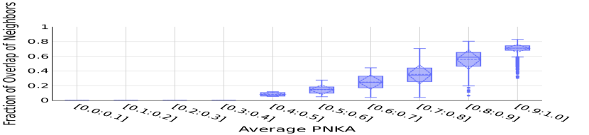
(a) $k$=500 (5% total points)

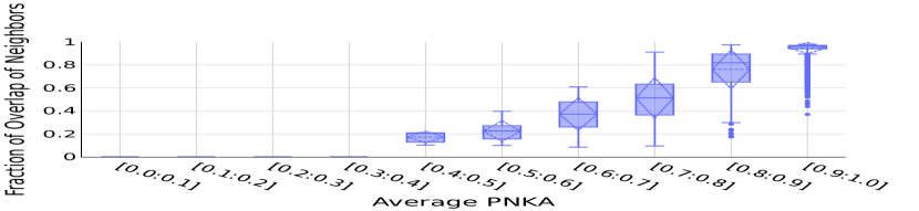
(b) $k$=1000 (10% total points)

Figure 1: PNKA captures the overlap of $k$ nearest neighbors between representations, i.e., the higher PNKA scores, the higher the fraction of overlapping neighbors. Results are an average over 3 runs, each one containing two ResNet-18 models trained on CIFAR-10 (25) with the same architecture but different random initialization.

In Section 2.1, we argue that for an input example to be similarly represented in two representations, its neighborhood should be similar across both of them. Here, we empirically show that this intuition applies to PNKA, and that if the PNKA score of point $i$ is higher than that of $j$, then $i$’s nearest neighbors in representations $Y$ and $Z$ overlap more than those of $j$. To show this, we train two ResNet-18 (19) models that only differ in their random initialization on the CIFAR-10 (25) dataset and compute their representations on the test set (10K instances). We use the penultimate layer (i.e., the layer before logits) for the remaining experiments of the paper. For each model, we determine a point’s $k$ nearest neighbors by ranking a point’s representation distance (via cosine similarity) to every other point in that representation. We then compute the fraction of those two sets of $k$ neighbors that intersect. Figure 1 depicts the relationship between PNKA similarity scores (x-axis) and the fraction of overlapping $k$ nearest neighbors of each point (y-axis), i.e. $1$ means all $k$ nearest neighbors are shared between both representations. Results are reported over 3 runs. We see a clear relationship between high PNKA scores and high overlap of nearest neighbors across representations, indicating that PNKA captures how similar the neighborhoods of the points are. In Appendix B.1.1 we show that this result generalizes to other architectures, datasets, distance measures, and values of $k$. We further show in Appendix B.1.2 that the direct comparison of representations through cosine similarity does not exhibit the same trend.

3.2 Relationship of PNKA with aggregate measures of representation similarity

PNKA is inspired by CKA’s idea of measuring similarity between representations by first computing the similarity between points within each of the representations and to then compare those similarity scores across the two representations. However, CKA and PNKA differ in how they compare similarity kernels across representations and, in contrast to PNKA, CKA only computes a single similarity score for all $N$ input examples. It can therefore not be used for the types of detailed analysis that PNKA enables. We can also use PNKA as an aggregate measure of representations similarity, as described in Equation 2. In Appendix B.2 we empirically demonstrate that the aggregate version of our measure ($\overline{\mbox{PNKA}}$) produces results that are similar to CKA.

3.3 Invariance properties

There is an ongoing discussion about which transformations representation similarity should be invariant to (11). Previous work (23) has identified invariance to orthogonal transformations and isotropic scaling as desirable properties for representation similarity measures. Here, we show that our measure possesses both of these invariance properties. See Appendix B.3 for proofs.

Invariance to orthogonal transformations.

Proposition 1.

Let $Y\in\mathbb{R}^{N\times k}$ and $Z\in\mathbb{R}^{N\times l}$ be two representations. Given two orthogonal matrices $Q\in\mathbb{R}^{k\times k}$ and $R\in\mathbb{R}^{l\times l}$, we have $\operatorname*{PNKA}(Y,Z,i)=\operatorname*{PNKA}(YQ,ZR,i)$, i.e. Pointwise Normalized Kernel Alignment is invariant to orthogonal transformation.

Invariance to isotropic scaling.

Proposition 2.

Let $Y\in\mathbb{R}^{N\times k}$ and $Z\in\mathbb{R}^{N\times l}$ be two representations. Given $\alpha,\beta\in\mathbb{R}$, we have $\operatorname*{PNKA}(Y,Z,i)=\operatorname*{PNKA}(\alpha Y,\beta Z,i)$, i.e. Pointwise Normalized Kernel Alignment is invariant to isotropic scaling.

4 Understanding representation similarity at finer granularity

We leverage the ability of PNKA to investigate representation similarity at a local level to gain a deeper understanding of how representation similarity is distributed across the test set, how it relates to other properties of models, such as their agreement in predictions, and to analyze a possible factor that might contribute to low representation similarity. Such analyses were previously not possible and we show how PNKA can help us gain interesting insights about model behavior at the granularity of individual data points.

4.1 Distinguishing similarly and dissimilarly represented inputs using PNKA

We use PNKA to better understand representation similarity in a more fine-grained manner in the context of one of the most important sanity checks in the literature: measuring representation similarity between models that only differ in their random initialization. Previous studies (23; 13; 33) have found the representations of two models that only differ in their random initialization to be quite similar, with CKA $>$ 0.9 at the penultimate layer (23). This result raises a number of questions: “is the (dis)similarity uniformly distributed among the representations of all points, or are there some very similar and dissimilar points?”, “what are the properties of (dis)similarly represented points?”, “does lower representation similarity imply higher disagreement on predictions?”. Existing representation similarity measures only provide aggregate estimates of similarity at a global level, and are thus not able to answer these questions.

We use PNKA to investigate the distribution of similarity scores across points and to relate it to the overall representation similarity on the entire test set. Figure 2(a) depicts the distribution of PNKA similarity scores. We show the average result over 3 different runs, each one containing two models trained on CIFAR-10 (25) with the same (ResNet-18 (19)) architecture but different random initialization. Figure 2(a) shows that most of the points exhibit high similarity scores, which aligns with the high CKA score (and $\overline{\mbox{PNKA}}$) obtained for the test set. However, the distribution of similarity scores is not uniform, and we observe that a few points achieve low similarity scores (on average 710 points have PNKA$<$0.85). Thus, even though the aggregate score of CKA (and $\overline{\mbox{PNKA}}$) indicates that overall the representations are similar, a small number of points are represented dissimilarly by the two models. In Appendix C.1 we expand this analysis to other architectures and datasets.

4.2 PNKA captures (dis-)agreement in model predictions

The ability of PNKA to provide pointwise similarity scores allows us to connect representation similarity to other metrics of model performance. A plausible hypothesis is that inputs with low similarity scores, i.e. inputs represented differently by the models, will also exhibit disagreement in their predictions. In Figure 2(b) we show that most of the points being dissimilarly represented are in fact the ones whose predictions the models disagree on the most. This result aligns with the intuition behind our measure since the connection between low similarity and disagreement can be explained by the differences in the neighborhoods for the points that achieve low similarity scores. We also show in Appendix C.3 that these points are not only classified in different ways but that most of them are misclassified as well. This result aligns with previous work on calibration (4; 21; 14) which uses a model’s outputs to detect which instances are more likely to be misclassified. In Appendix C.2, we show the same pattern for other choices of architecture and dataset.

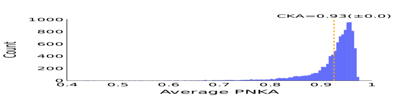
(a) Distribution of PNKA.

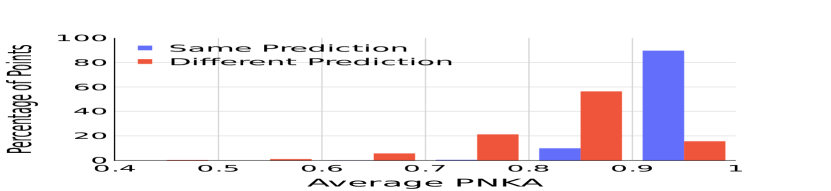
(b) Distribution of PNKA per Prediction.

Figure 2: Distribution of PNKA similarity scores. Results are an average over 3 runs, each one containing two models trained on CIFAR-10 (25) with the same architecture (ResNet-18 (19)) but different random initialization. The average standard deviation is $0.022$. Left: while most of the points are similarly represented (which agrees with CKA score), some are dissimilarly represented. Right: points being dissimilarly represented are the ones whose predictions the models disagree on the most.

4.3 Out of distribution inputs are dissimilarly represented

The previous results show that there are a few points with dissimilar representations in the test set of a standard classification task. This raises the question: “what leads to dissimilarly represented points?”. Prior work (13) observed that CKA can detect out-of-distribution (OOD) data differences without access to OOD data, i.e., CKA similarity scores are low for OOD data. However, since aggregate measures were used for this study, a more comprehensive analysis at the level of data points was not possible. Here we hypothesize that the representations of models agree on points that have a high likelihood under the models’ training distributions, but that the representations of models will disagree on OOD points. To test this hypothesis, we deliberately perturb a number of points in the test set  such that they differ from the training samples. We then compute PNKA on the test set with $p\%$ perturbed and $1-p\%$ non-perturbed (i.e. original) points for models that differ in their random initialization. In Figure 3 we use $p=10\%$ and show that, for different types of perturbations, perturbed points obtain low similarity scores compared to the original points. We expand this analysis for other choices of $p$ in Appendix C.4.

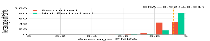
(a) Blurring.

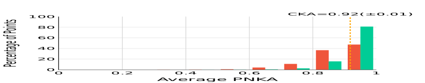
(b) Elastic Transform.

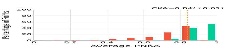
(c) Adversarial Perturbation.

Figure 3: Perturbed points in the test set obtain lower similarity scores than non-perturbed (i.e. original) points for different types of perturbations. We use $p\%$ perturbed and $1-p\%$ non-perturbed points, where $p=10$ in this case. Results are an average over 3 runs, each one containing two models trained on CIFAR-10 (25) with the same architecture (ResNet-18 (19)) but different random initialization.

5 PNKA as an interpretability tool

PNKA can be useful as a tool for model interpretability. In this Section, we showcase its use for interpreting the role of individual neurons in a representation. To understand what a specific neuron in a given layer is capturing, we can compare the representations of the full layer (with all neurons) to the representations of the layer without the neuron. We can then observe how omitting the neuron affects the representation of each input in the test set, i.e. the lower the PNKA score for an input $i$, the more its representation is altered by the removal of the neuron. Thus, by inspecting and visualizing the least similar inputs when removing the neuron, one can gain insights into what patterns make a neuron’s response unique from other neurons. We use this method to interpret what unique features the neurons at the penultimate layer of a ResNet-18 model (19) are capturing. We observe that some images obtain low similarity scores for some of the neurons removed and that most of those images pertain to one or two classes (shown in Appendix D.1). This indicates that the neurons in the penultimate layer are highly specialized in capturing features at the level of classes.

	Overall	Airplane	Automobile	Bird	Cat	Deer	Dog	Frog	Horse	Ship	Truck
Random	0.950	0.962	0.959	0.909	0.822	0.962	0.898	0.926	0.934	0.954	0.961
(Most Aligned) Target Class	-	0.994	0.996	0.994	0.983	0.997	0.982	0.990	0.996	0.991	0.989
(Least Aligned) Target Class	-	0.596	0.423	0.018	0.000	0.000	0.263	0.000	0.000	0.000	0.176

Table 1: Accuracy results of linear probes on the 50 neurons that most (least) align with a specific class obtain higher (lower) accuracy compared to randomly picking neurons (full table in Appendix D.2).

To validate the observation that many neurons primarily correspond to specific classes, for each class, we select $\approx$10% (50) of the neurons that have the highest ratio of images from that class in the 100 inputs that changed the most and train a linear probe on those. These neurons are the ones that best capture each class. Our hypothesis is that, if the 50 neurons are indeed capturing unique information about that class, the accuracy will increase significantly for that specific class. We also run the same experiment for the 50 neurons that least capture the corresponding classes as a baseline. Tab. 1 shows that the models trained with the 50 most (least) informative neurons of a specific class achieve a higher (lower) accuracy for that class compared to the one that randomly selects 50 neurons. We additionally compare these results with other work in the literature (7; 5), which analyzes the activations of neurons (i.e. the more a neuron activates, the more that neuron is excited by the features on those images), and show that both methods achieve similar results. However, while looking at activations show how much each neuron triggers for each input $i$, and can only be applied to this specific context, our method informs what unique images, and features, each neuron is capturing, and can be generally applied to different contexts. PNKA can be further used to analyze how the model changes with respect to space (i.e. across layers) or time (i.e. across epochs). We leave this for future investigation.

6 Using PNKA to analyze model interventions

Our measure can also be used as a tool to understand the effects of interventions on a model. We can use PNKA to compute pointwise similarity scores between the representations of the original and the modified (i.e. intervened) models and analyze the inputs that are most affected by the intervention. We now showcase the use of PNKA in the context of interventions to learn fair ML models.

An important goal of fair ML literature is non-discrimination, where we attempt to mitigate biases that affect protected groups in negative ways (2; 36). A popular approach to achieve non-discrimination is through learning debiased or fair representations (48; 9; 30). These approaches transform or train model representations in a way that minimizes the information they contain about the group membership of inputs. However, today, we often overlook how the interventions targeting (macro-)group-level fairness affect representations at the (micro-)individual-level and whether the changes in individual point representations are desirable or as intended. By applying PNKA to the original and the debiased representations, we can understand the effects of the debiasing intervention at the level of individual inputs, and analyze the inputs whose representations underwent the biggest change. We demonstrate how this ability can be leveraged in the context of natural language word embeddings to investigate whether the debiasing approaches indeed work as intended.

Approaches to debias word embeddings: Many word embedding approaches have been found to produce biased representations with stereotypical associationss (6; 16; 49), and several methods have been proposed with the goal of reducing these stereotypical biases (6; 16; 49; 22). In this work, we choose two of such debiasing approaches with the goal of using PNKA to analyze whether debiasing successfully decreases stereotypical associations. Both debiasing techniques are based on the original GloVe (22): (1) Gender Neutral (GN-)GloVe (49) focuses on disentangling and isolating all the gender information into certain specific dimension(s) of the word vectors; (2) Gender Preserving (GP-)GloVe (22) targets preserving non-discriminative gender-related information while removing stereotypical discriminative gender biases from pre-trained word embeddings. The latter method can also be used to finetune GN-GloVe embeddings, generating another model namely, GP-GN-GloVe.

Evaluation of debiased word embeddings: In order to evaluate the impact of the debiasing methods, both GP- and GN-GloVe use the SemBias dataset (49). Each instance in SemBias consists of four word pairs: a gender-definition word pair (e.g. “waiter - waitress”), a gender-stereotype word pair (e.g. “doctor - nurse”), and two other word-pairs that have similar meanings but no gender relation, named gender-neutral (e.g. “dog - cat”). The goal is to evaluate whether the debiasing methods have successfully removed stereotypical gender information from the word embeddings, while simultaneously preserving non-stereotypical gender information. To this end, GP- and GN-GloVe evaluated how well the embeddings can be used to predict stereotypical word pairs in each instance of the SemBias dataset. The details and results of this prediction task are in Appendix E.1. The evaluation shows that GP-Golve embeddings offer only a marginal improvement, while GN-GloVe and GP-GN-GloVe embeddings offer substantial improvement at the prediction task.

Using PNKA to understand debiased word embeddings: We applied PNKA to the original and the debiased GloVe embeddings to examine whether the methods are indeed reducing bias as claimed. Figure 4 shows the distribution of PNKA scores for words in SemBias dataset grouped by their category (i.e., gender defining, gender neutral, and gender stereotype). We highlight two observations. First, GP-Glove representations are very similar to GloVe (Figure4(a)) for almost all of the words, whereas GN-Glove (Figure4(b)) and GP-GN-GloVe (Figure4(c)) considerably change the representations for a subset set of the words. This observation aligns well with results of prior evaluation which found that GP-GloVe achieves similar results to GloVe, while GN-Glove and GP-GN-Glove achieve better debiasing results. Second, Figure 4 also shows that across all three debiasing methods, the words whose embeddings change the most are the gender-definition words. Note that this observation is in complete contradiction to the expectation that with debiasing, the embeddings that would change the most are the gender-stereotypical ones, while the embeddings that would be preserved and not change are the gender-definitional ones. Put differently, our PNKA similarity scores suggest a very different explanation for why GN-GloVe and GP-GN-GloVe achieve better debiasing evaluation results over SemBias dataset: rather than remove gender information from gender-stereotypical word pairs, they are amplifying the gender information in gender-definition word pairs, resulting in better performance in distinguishing gender-stereotypical and gender-definition word pairs.

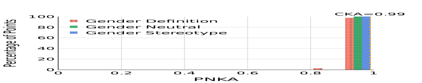
(a) GloVe $\times$ GP-GloVe.

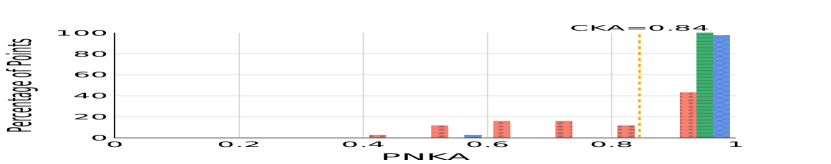
(b) GloVe $\times$ GN-GloVe.

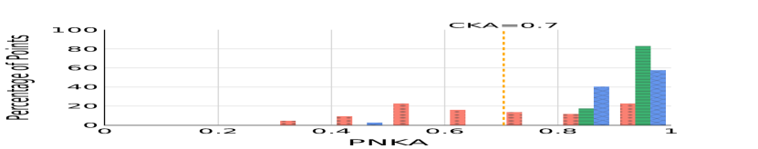
(c) GloVe $\times$ GP-GN-GloVe.

Figure 4: Distribution of PNKA scores per group of words for SemBias dataset (49). We compare the baseline (GloVe) model and its debiased versions. Words with the lowest similarity scores are the ones that change the most from the baseline to its debiased version. Across all debiased embeddings, the words whose embeddings change the most are the gender-definition word.

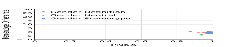
(a) GloVe $\times$ GP-GloVe.

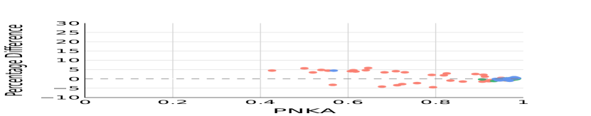
(b) GloVe $\times$ GN-GloVe.

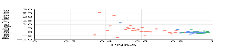
(c) GloVe $\times$ GP-GN-GloVe.

Figure 5: Relationship between PNKA scores and percentage change in magnitude of the projection onto the gender vector from the baseline GloVe. A positive change indicates an increase in magnitude along the canonical gender direction. Word embeddings that change their gender information are the ones that obtain low PNKA scores.

We confirm our alternate explanation by measuring for each word how much its embedding changed in terms of gender information, when compared to the original GloVe embedding, by projecting it onto the canonical gender vector $\overrightarrow{he}$ - $\overrightarrow{she}$ (more details in Appendix E.2), generating the percentage difference in magnitude. Figure 5 shows that the GN-GloVe and GP-GN-GloVe debiasing methods primarily amplify the gender information in gender-definition words, rather than reduce it for gender-stereotype words. In fact, the words that change their gender information the most are the low-similarity ones. This analysis illustrates how PNKA’s pointwise similarity scores can offer new insights, trigger new investigations, and lead to a better understanding of the effects of model training interventions.

7 Conclusion

In this work, we proposed Pointwise Normalized Kernel Alignment (PNKA), a measure of representation similarity of individual data points. PNKA provides a distribution of similarity scores that in aggregate matches global representation similarity measures, and thus, can be seen as a local decomposition of the global score. We showed that our method possesses several intriguing properties and offers an intuitive depiction of neighborhood similarity across representations. Using PNKA we showed that not all the data points obtain a high similarity score in a context where aggregated measures provide a high overall similarity score, and we relate this finding to other model properties, such as their agreement, and data characteristics, such as its distribution. Furthermore, we illustrate how PNKA serves as an interpretability tool, enabling a better understanding of the semantics associated with individual neurons in a representation. Expanding upon this line of analysis, one could explore spatial variations across layers or temporal dynamics across epochs within the model. Finally, we used the context of fairness to show that PNKA can be a useful tool for understanding which points are most affected by model interventions, thus shedding light on the internal characteristics of such modifications. Future investigations may extend to exploring other types of model interventions, such as assessing model interventions in the domain of robustness against adversarial attacks. A limitation of our work lies in the restricted consideration of only a few model variations, with an exclusive focus on the penultimate layer.

Appendix A Training details

The models used in this paper were trained for 1 GPU day on Nvidia A40 and for 1 GPU day on Nvidia A100, in an on-premise cluster. We train models with ResNet-18 [19], VGG-16  and Inception-V3  architectures on CIFAR-10 and CIFAR-100 [25] datasets. All models were trained with weight decay of $5e-4$, learning rate of $0.1$ and learning rate step of $50$. All models were trained for $150$ epochs, saving the checkpoint with the best (i.e. highest) validation accuracy. We used SGD optimizer for all models, with SGD momentum of $0.9$. We report in Table 2 the overall accuracy of each model.

Dataset	Model	Seed	Accuracy
CIFAR-10	ResNet-18	0	0.9508
		1	0.9463
		2	0.9528
		3	0.9488
		4	0.9507
		5	0.9486
	VGG-16	0	0.9349
		1	0.9341
		2	0.9362
		3	0.9351
		4	0.9308
		5	0.9359
	Inception-V3	0	0.9495
		1	0.9493
		2	0.9504
		3	0.9472
		4	0.9476
		5	0.9518
CIFAR-100	ResNet-18	0	0.7713
		1	0.7729
		2	0.7722
		3	0.7722
		4	0.7763
		5	0.7719
	VGG-16	0	0.7293
		1	0.7295
		2	0.7298
		3	0.7284
		4	0.7338
		5	0.7287
	Inception-V3	0	0.7850
		1	0.7836
		2	0.7892
		3	0.7926
		4	0.7888
		5	0.7910

Table 2: Overall accuracy for each the models used in our analysis.

Appendix B Properties

B.1 Overlap of neighbors

In Section 2.1, we argue that for an input example to be similarly represented in two representations, its neighborhood should be similar across both of them. Here, we empirically show that this intuition applies to PNKA, and that if the PNKA score of point $i$ is higher than that of $j$, then $i$’s nearest neighbors in representations $Y$ and $Z$ overlap more than those of $j$. To show this, we train two models that only differ in their random initialization and compute their representations on the test set (10K instances). We use the penultimate layer (i.e., the layer before logits) for the analysis. For each model, we determine a point’s $k$ nearest neighbors by ranking a point’s representation distance (via either cosine similarity or L2 distance) to every other point in that representation. We then compute the fraction of those two sets of $k$ neighbors that intersect.

In the following plots we depicts the relationship between PNKA similarity scores (x-axis) and the fraction of overlapping $k$ nearest neighbors of each point (y-axis), i.e. $1$ means all $k$ nearest neighbors are shared between both representations. We report the analysis on CIFAR-10 and CIFAR-100 [25], for ResNet-18 [19], VGG-16 and Inception-V3, for different $k$ values, up to $k=20\%$ of the dataset size. All the results are reported over 3 runs. In all cases of Section B.1.1 we see a clear relationship between high PNKA scores and high overlap of nearest neighbors across representations, indicating that PNKA captures how similar the neighborhoods of the points are. We further show in Section B.1.2 that the direct comparison of representations through cosine similarity does not exhibit the same trend, i.e. there is not a positive correlation between cosine similarity scores and the fraction of overlap of the $k$ nearest neighbors.

B.1.1 Additional results for PNKA

CIFAR-10, determining nearest neighbors via cosine similarity

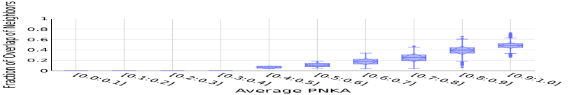
(a) ResNet-18, $k$=250 (2.5% total points)

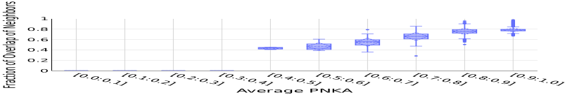
(b) ResNet-18, $k$=2000 (20% total points)

(c) VGG-16, $k$=250 (2.5% total points)

(d) VGG-16, $k$=500 (5% total points)

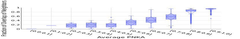
(e) VGG-16, $k$=1000 (10% total points)

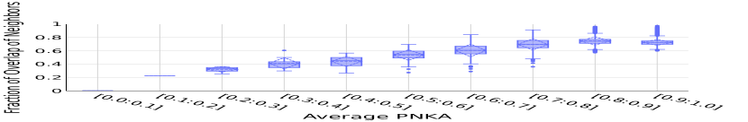
(f) VGG-16, $k$=2000 (20% total points)

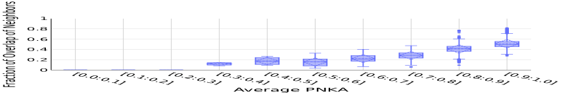
(g) Inception-V3, $k$=250 (2.5% total points)

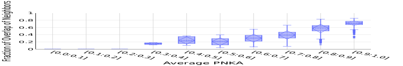
(h) Inception-V3, $k$=500 (5% total points)

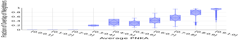
(i) Inception-V3, $k$=1000 (10% total points)

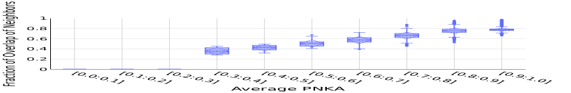
(j) Inception-V3, $k$=2000 (20% total points)

Figure 6: PNKA captures the overlap of $k$ nearest neighbors between two representations, i.e., the higher PNKA scores, the higher the fraction of overlapping neighbors. Results are an average over 3 runs, each one containing two models trained on CIFAR-10 [25] dataset with the same architecture but different random initialization.

CIFAR-100, determining nearest neighbors via cosine similarity

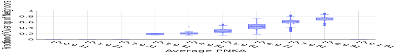
(a) ResNet-18, $k$=250 (2.5% total points)

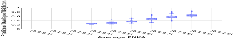
(b) ResNet-18, $k$=500 (5% total points)

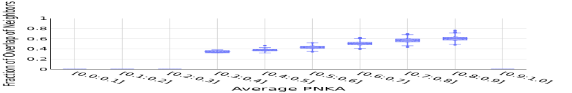
(c) ResNet-18, $k$=1000 (10% total points)

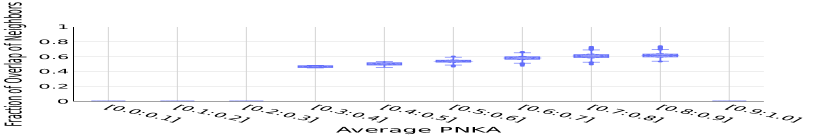
(d) ResNet-18, $k$=2000 (20% total points)

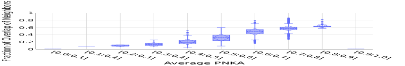
(e) VGG-16, $k$=250 (2.5% total points)

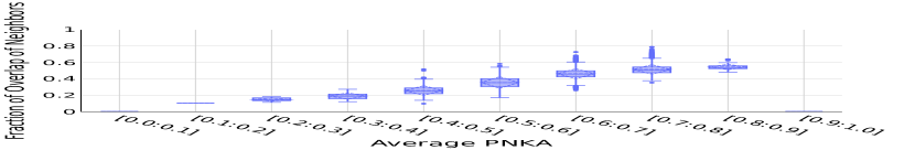
(f) VGG-16, $k$=500 (5% total points)

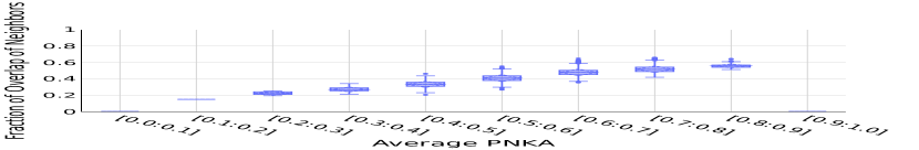
(g) VGG-16, $k$=1000 (10% total points)

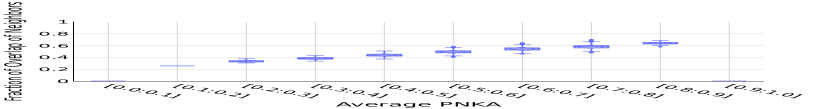
(h) VGG-16, $k$=2000 (20% total points)

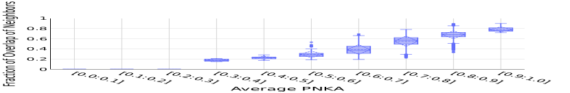
(i) Inception-V3, $k$=250 (2.5% total points)

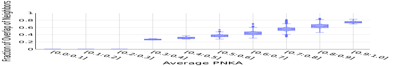
(j) Inception-V3, $k$=500 (5% total points)

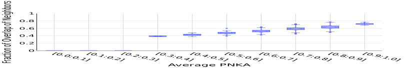
(k) Inception-V3, $k$=1000 (10% total points)

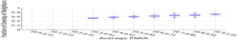
(l) Inception-V3, $k$=2000 (20% total points)

Figure 7: PNKA captures the overlap of $k$ nearest neighbors between two representations, i.e., the higher PNKA scores, the higher the fraction of overlapping neighbors. Results are an average over 3 runs, each one containing two models trained on CIFAR-100 [25] dataset with the same architecture but different random initialization.

CIFAR-10, determining nearest neighbors via L2 distance

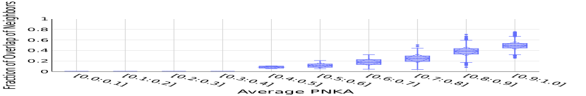
(a) ResNet-18, $k$=250 (2.5% total points)

(b) ResNet-18, $k$=500 (5% total points)

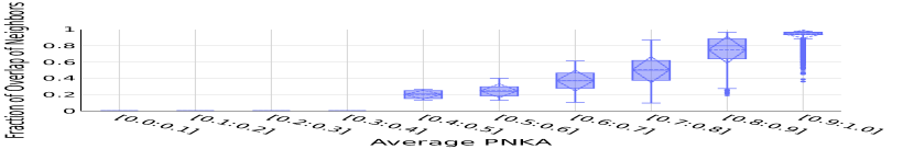
(c) ResNet-18, $k$=1000 (10% total points)

(d) ResNet-18, $k$=2000 (20% total points)

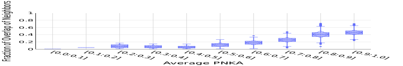
(e) VGG-16, $k$=250 (2.5% total points)

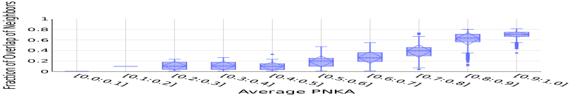
(f) VGG-16, $k$=500 (5% total points)

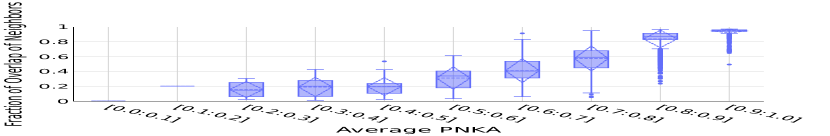
(g) VGG-16, $k$=1000 (10% total points)

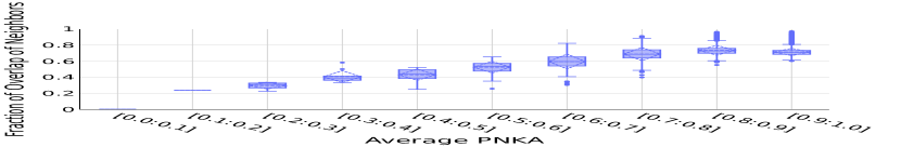
(h) VGG-16, $k$=2000 (20% total points)

Figure 8: PNKA captures the overlap of $k$ nearest neighbors between two representations, i.e., the higher PNKA scores, the higher the fraction of overlapping neighbors. Results are an average over 3 runs, each one containing two models trained on CIFAR-10 [25] dataset with the same architecture but different random initialization.

CIFAR-100, determining nearest neighbors via L2 distance

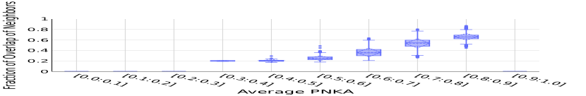
(a) ResNet-18, $k$=250 (2.5% total points)

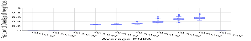
(b) ResNet-18, $k$=500 (5% total points)

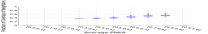
(c) ResNet-18, $k$=1000 (10% total points)

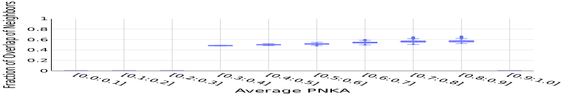
(d) ResNet-18, $k$=2000 (20% total points)

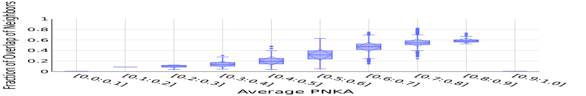
(e) VGG-16, $k$=250 (2.5% total points)

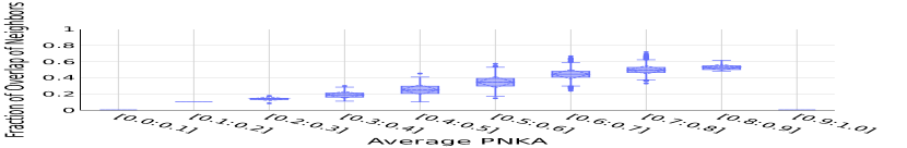
(f) VGG-16, $k$=500 (5% total points)

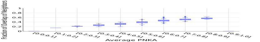
(g) VGG-16, $k$=1000 (10% total points)

(h) VGG-16, $k$=2000 (20% total points)

Figure 9: PNKA captures the overlap of $k$ nearest neighbors between two representations, i.e., the higher PNKA scores, the higher the fraction of overlapping neighbors. Results are an average over 3 runs, each one containing two models trained on CIFAR-100 [25] dataset with the same architecture but different random initialization.

B.1.2 Cosine similarity is not able to capture the overlap of neighbors

CIFAR-10, determining nearest neighbors via cosine similarity

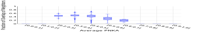
(a) ResNet-18, $k$=250 (2.5% total points)

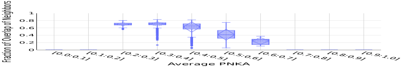
(b) ResNet-18, $k$=500 (5% total points)

(c) ResNet-18, $k$=1000 (10% total points)

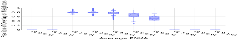
(d) ResNet-18, $k$=2000 (20% total points)

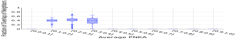
(e) VGG-16, $k$=100 (2.5% total points)

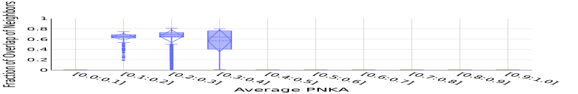
(f) VGG-16, $k$=500 (5% total points)

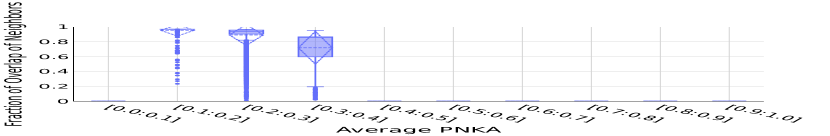
(g) VGG-16, $k$=1000 (10% total points)

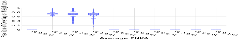
(h) VGG-16, $k$=2000 (20% total points)

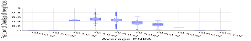
(i) Inception-V3, $k$=250 (2.5% total points)

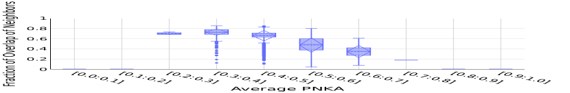
(j) Inception-V3, $k$=500 (5% total points)

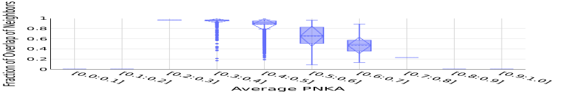
(k) Inception-V3, $k$=1000 (10% total points)

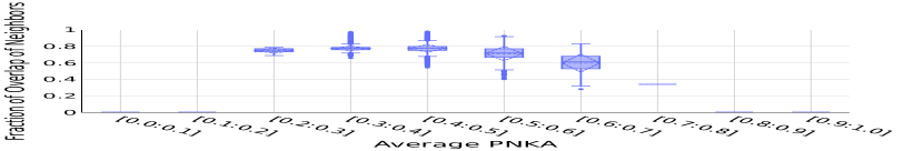
(l) Inception-V3, $k$=2000 (20% total points)

Figure 10: Cosine similarity is not able to captures the overlap of $k$ nearest neighbors between two representations i.e. there is not a positive correlation between cosine similarity scores and the fraction of overlap of the $k$ nearest neighbors. Results are an average over 3 runs, each one containing two models trained on CIFAR-10 [25] dataset with the same architecture but different random initialization.

CIFAR-100, determining nearest neighbors via cosine similarity

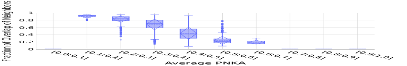
(a) ResNet-18, $k$=100 (1% total points)

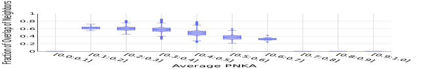
(b) ResNet-18, $k$=500 (5% total points)

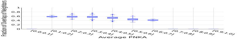
(c) ResNet-18, $k$=1000 (10% total points)

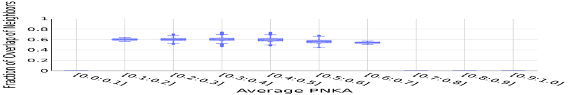
(d) ResNet-18, $k$=2000 (20% total points)

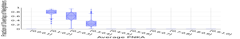
(e) VGG-16, $k$=100 (1% total points)

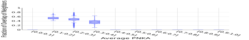
(f) VGG-16, $k$=500 (5% total points)

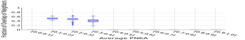
(g) VGG-16, $k$=1000 (10% total points)

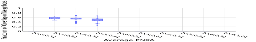
(h) VGG-16, $k$=2000 (20% total points)

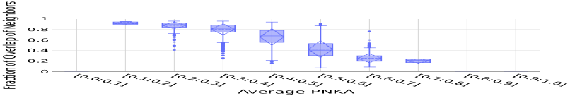
(i) Inception-V3, $k$=100 (1% total points)

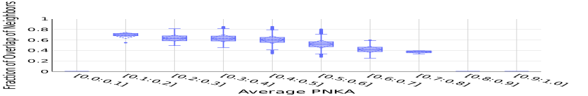
(j) Inception-V3, $k$=500 (5% total points)

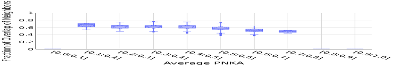
(k) Inception-V3, $k$=1000 (10% total points)

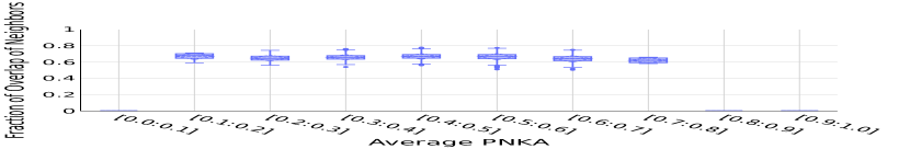
(l) Inception-V3, $k$=2000 (20% total points)

Figure 11: Cosine similarity is not able to captures the overlap of $k$ nearest neighbors between two representations i.e. there is not a positive correlation between cosine similarity scores and the fraction of overlap of the $k$ nearest neighbors. Results are an average over 3 runs, each one containing two models trained on CIFAR-100 [25] dataset with the same architecture but different random initialization.

B.2 Relationship of PNKA with aggregate measures of representation similarity

Dataset	Model	CKA	$\overline{\mbox{PNKA}}$
CIFAR-10	ResNet-18	0.925 (±0.005)	0.925 (±0.022)
	VGG-16	0.895 (±0.013)	0.893 (±0.039)
	Inception-v3	0.916 (±0.001)	0.915 (±0.023)
CIFAR-100	ResNet-18	0.741 (±0.00)	0.733 (±0.033)
	VGG-16	0.658 (±0.010)	0.668 (±0.049)
	Inception-v3	0.798 (±0.009)	0.792 (±0.032)

Table 3: Comparison between CKA [23] and the aggregate version of PNKA ($\overline{\mbox{PNKA}}$). Results are an average over 3 runs, each one with two models that only differ in their random initialization. We capture the representations of the penultimate layer (i.e., the layer before logits) for the analysis. We show that both measures produce similar overall scores.

B.3 Proof of invariances

B.3.1 Invariance to orthogonal transformations

Proof.

It suffices to show that

$$K(YQ) =YQ(YQ)^{\top}$$

$$=YQQ^{\top}Y^{\top}$$

$$=YQQ^{-1}Y^{\top}$$

$$=YY^{\top}$$

$$=K(Y)$$

Here we have used that for an orthogonal matrix $Q$, $Q^{\top}=Q^{-1}$. By substituting $K(YQ)$ and $K(ZR)$ in $\operatorname*{PNKA}(YQ,ZR,i)=\cos(K(YQ)_{i},K(ZR)_{i})$ with $K(Y)$ and $K(Z)$, respectively, we obtain $\operatorname*{PNKA}(YQ,ZR,i)=\operatorname*{PNKA}(Y,Z,i)$. Thus, PNKA is invariant to orthogonal transformations. ∎

B.3.2 Invariance to isotropic scaling

Proof.

Note that because of the bilinearity of the dot-product, we have $K(\alpha Y)_{i}=\left[(\alpha Y)(\alpha Y)^{\top}\right]_{i}=\alpha^{2}K(Y)_{i}$. By substituting into $\operatorname*{PNKA}$, we get

$$\operatorname*{PNKA}(\alpha Y,\beta Z,i) =\frac{K(\alpha Y)_{i}^{\top}K(\beta Z)_{i}}{||K(\alpha Y)_{i}||_{2}||K(\beta Z)_{i}||_{2}}$$

$$=\frac{\alpha^{2}K(Y)_{i}^{\top}\beta^{2}K(Z)}{||\alpha^{2}K(Y)_{i}||_{2}||\beta^{2}K(Z)_{i}||_{2}}$$

$$=\frac{\alpha^{2}K(Y)_{i}^{\top}\beta^{2}K(Z)}{\alpha^{2}||K(Y)_{i}||_{2}\beta^{2}||K(Z)_{i}||_{2}}$$

$$=\operatorname*{PNKA}(Y,Z,i).$$

Thus, PNKA is invariant to isotropic scaling. ∎

Appendix C Understanding representation similarity at finer granularity

C.1 Distinguishing similarly and dissimilarly represented inputs using PNKA

We use PNKA to investigate the distribution of similarity scores across points and to relate it to the overall representation similarity on the entire test set. In Section C.1.1 we show the distribution of PNKA similarity scores for ResNet-18, VGG-16 and Inception-V3, for both CIFAR-10 and CIFAR-100 datasets. We show the average result over 3 different runs, each one containing two models with the same architecture but different random initialization. We show that in all cases, most of the points exhibit high similarity scores, which aligns with the high CKA score (and $\overline{\mbox{PNKA}}$) obtained for the test set. However, the distribution of similarity scores is not uniform, and we observe that a few points achieve low similarity scores. We also visualize some of the low similarity instances of CIFAR-10 in Section C.1.2.

C.1.1 Additional PNKA scores distribution

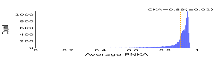
(a) VGG-16, CIFAR-10.

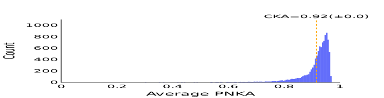
(b) Inception-V3, CIFAR-10.

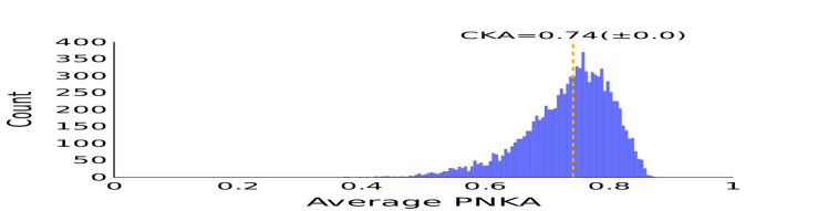
(c) ResNet-18, CIFAR-100.

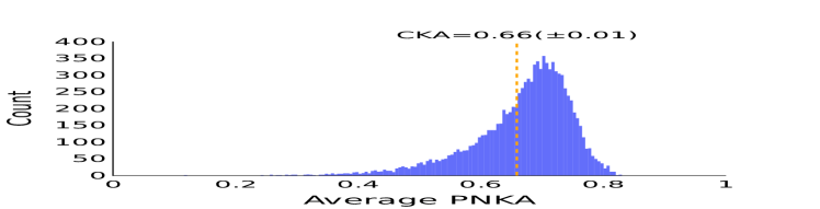
(d) VGG-16, CIFAR-100.

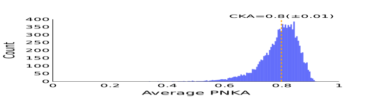
(e) Inception-V3, CIFAR-100.

Figure 12: Distribution of PNKA similarity scores. Results are an average over 3 runs, each one containing two models with the same architecture but different random initialization. While most of the points are similarly represented (which explains the high aggregate CKA and $\overline{\mbox{PNKA}}$ scores), some are dissimilarly represented.

C.1.2 Visualizing images with the lowest PNKA scores

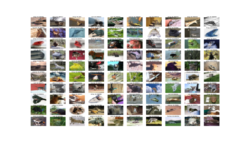
(a) ResNet-18.

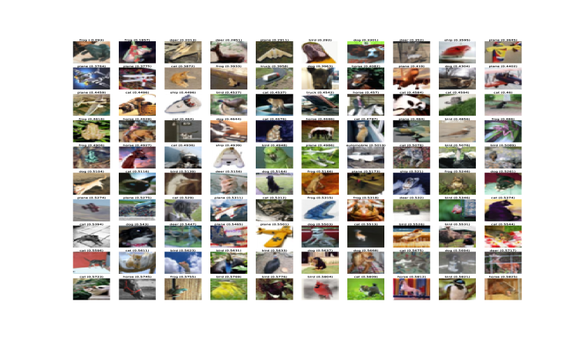
(b) VGG-16.

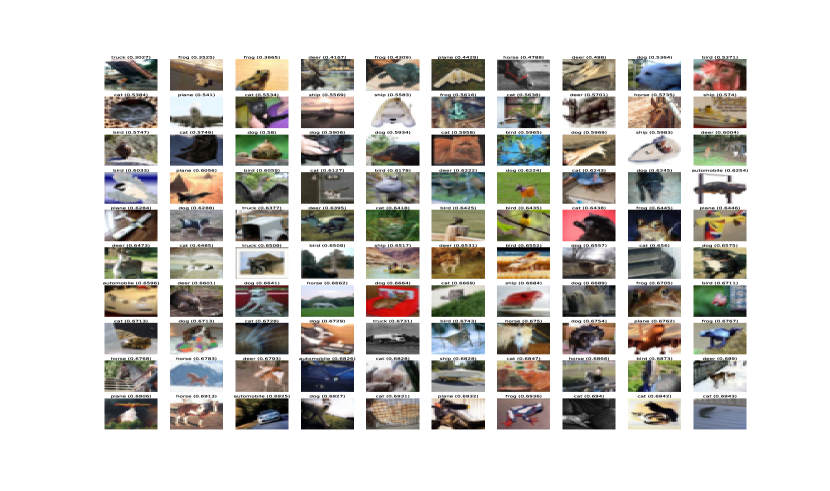
(c) Inception-V3.

Figure 13: Images with the lowest PNKA score. Results are an average over 3 runs, each one containing two models trained on CIFAR-10 [25] with the same architecture but different random initialization.

C.2 PNKA captures (dis-)agreement in model predictions

The ability of PNKA to provide pointwise similarity scores allows us to connect representation similarity to other metrics of model performance. A plausible hypothesis is that inputs with low similarity scores, i.e. inputs represented differently by the models, will also exhibit disagreement in their predictions. In this Section, we show the same pattern for more choices of architecture and dataset. We consider the “same prediction” when all the 6 models (2 for each run) agree on the label of the prediction. In Figure 14 we show that most of the points being dissimilarly represented are in fact the ones whose predictions the models disagree on the most. This result aligns with the intuition behind our measure since the connection between low similarity and disagreement can be explained by the differences in the neighborhoods for the points that achieve low similarity scores.

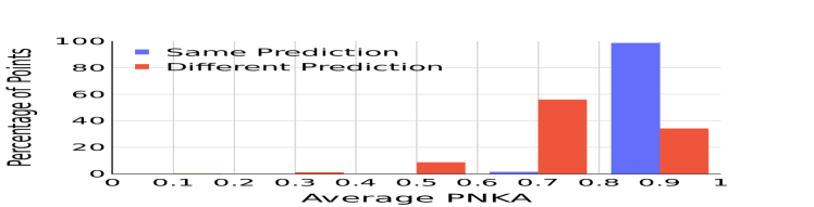
(a) VGG-16, CIFAR-10.

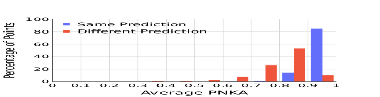
(b) Inception-V3, CIFAR-10.

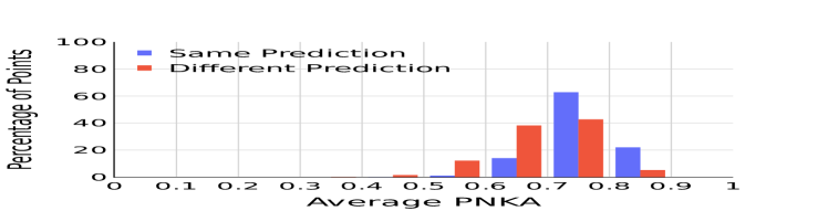
(c) ResNet-18, CIFAR-100.

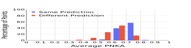
(d) VGG-16, CIFAR-100.

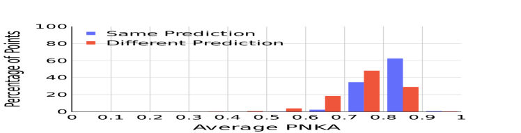
(e) Inception-V3, CIFAR-100.

Figure 14: Distribution of PNKA similarity scores, i.e. the blue (“same prediction”) and red (“different prediction”) bars have been normalized separately to sum up to 100. Results are an average over 3 runs, each one containing two models with the same architecture but different random initialization. We consider the “same prediction” when all the 6 models (2 for each run) agree on the label of the prediction. Points being dissimilarly represented are the ones whose predictions the models disagree on the most.

C.3 Dissimilar points are more likely to be misclassified

In this Section (Figure 15), we show that the points being dissimilarly represented are more likely to be misclassified by the models. We consider a “correct prediction” as one where all the 6 models (2 for each run) correctly predict the ground-truth label. Results are an average over 3 runs, each one containing two models with the same architecture but different random initialization.

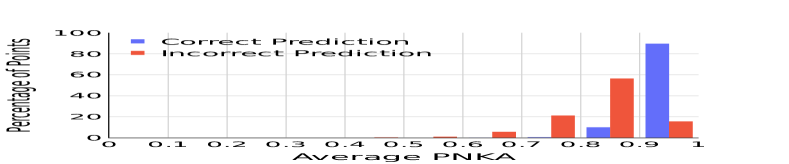
(a) ResNet-18, CIFAR-10.

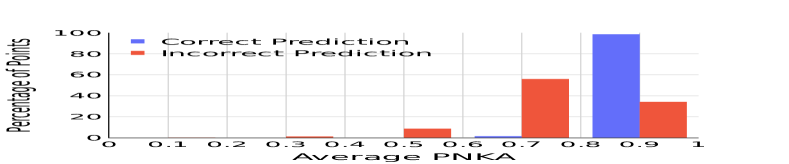
(b) VGG-16, CIFAR-10.

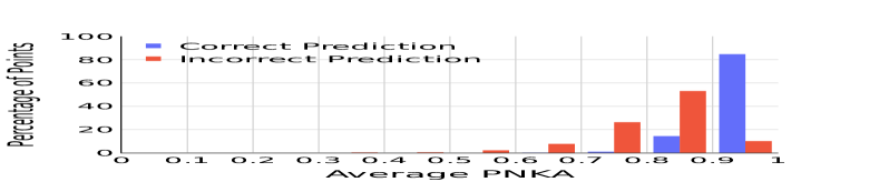
(c) Inception-V3, CIFAR-10.

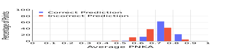
(d) ResNet-18, CIFAR-100.

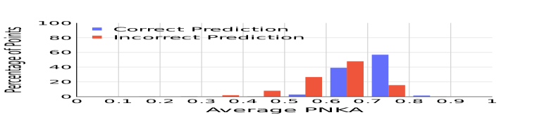
(e) VGG-16, CIFAR-100.

(f) Inception-V3, CIFAR-100.

Figure 15: Distribution of PNKA similarity scores, i.e. the blue (“correct prediction”) and red (“incorrect prediction”) bars have been normalized separately to sum up to 100. Results are an average over 3 runs, each one containing two models with the same architecture but different random initialization. A correct prediction is when all the 6 models (2 for each run) correctly predict the ground-truth label. Points being dissimilarly represented are the ones whose predictions the models misclassify the most.

C.4 Out of distribution inputs are dissimilarly represented

In this section, we provide additional analysis on the out-of-distribution (OOD) experiment of Section 4.3. For constructing adversarial images, we use the ‘robustness’ package  with the PGD attack . We use $100$ attacks steps, epsilon of $1$ and step size of $0.5$, so that the attacked model has accuracy of $\approx 0$ in the generated images. For both blurring and elastic transformations, we used the torchvision package. We set the kernel size to $9\times 9$ and a sigma from $0.5$ to $2.5$ for the Gaussian blur. Finally, we set the alpha to $80$ for the elastic transformation. We use $p\%$ perturbed and $(100-p)\%$ non-perturbed points. We show that OOD points are more likely to be dissimilarly represented, for different datasets, architectures, and $p$ values. Results are an average over 3 runs, each one containing two models with the same architecture but different random initialization.

C.4.1 Blurring perturbations

CIFAR-10

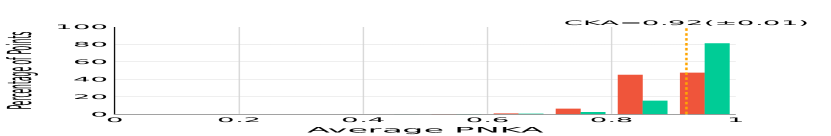
(a) R18, $p=50\%$.

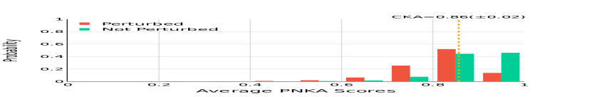
(b) R18, $p=50\%$.

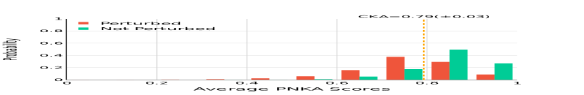
(c) R18, $p=90\%$.

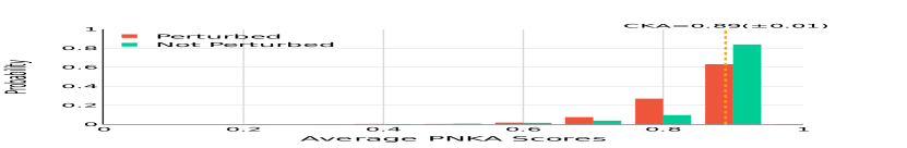
(d) VGG16, $p=10\%$.

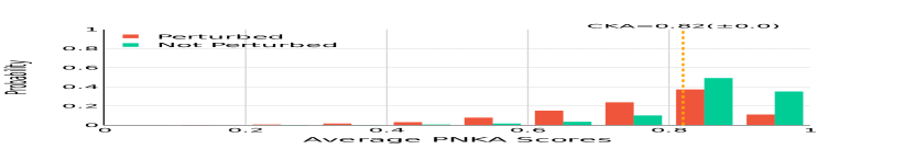
(e) VGG16, $p=50\%$.

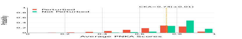
(f) VGG16, $p=90\%$.

Figure 16: Perturbed points in the test set are more likely to obtain lower similarity scores than non-perturbed (i.e. original) points for blurring. We use $p\%$ perturbed and $100-p\%$ non-perturbed points. Results are an average over 3 runs, each one containing two models trained on CIFAR-10 [25] with the same architecture but different random initialization.

CIFAR-100

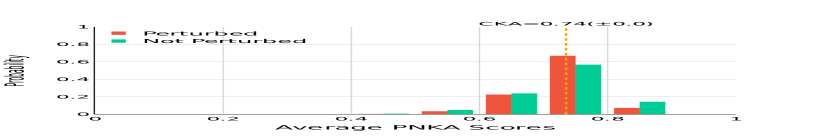
(a) R18, $p=10\%$.

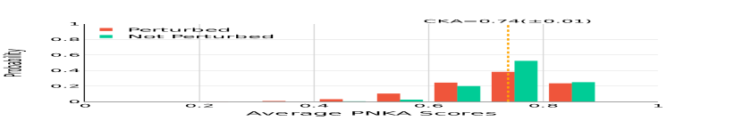
(b) R18, $p=50\%$.

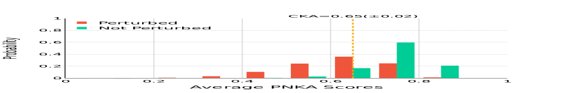
(c) R18, $p=90\%$.

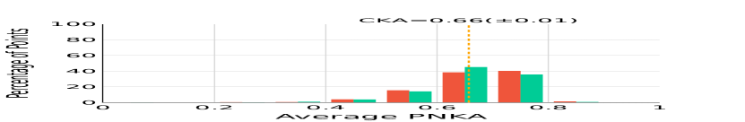
(d) VGG16, $p=10$.

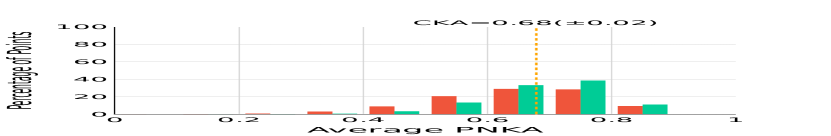
(e) VGG16, $p=50\%$.

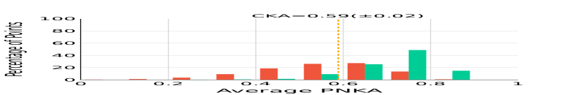
(f) VGG16, $p=90\%$.

Figure 17: Perturbed points in the test set are more likely to obtain lower similarity scores than non-perturbed (i.e. original) points for blurring. We use $p\%$ perturbed and $100-p\%$ non-perturbed points. Results are an average over 3 runs, each one containing two models trained on CIFAR-100 [25] with the same architecture but different random initialization.

C.4.2 Elastic perturbations

CIFAR-10

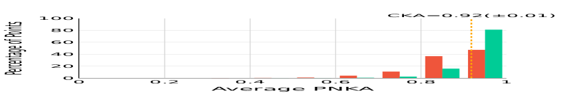
(a) R18, $p=10\%$.

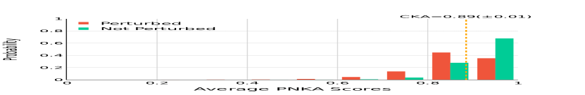
(b) R18, $p=50\%$.

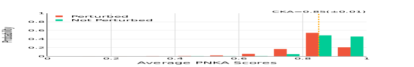
(c) R18, $p=90\%$.

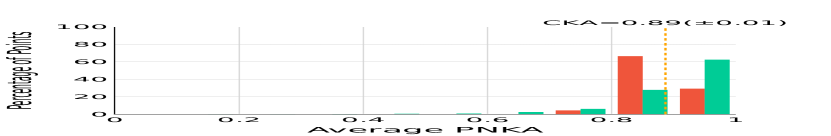
(d) VGG16, $p=10\%$.

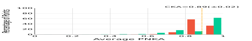
(e) VGG16, $p=50\%$.

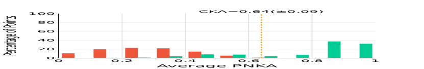
(f) VGG16, $p=90\%$.

Figure 18: Perturbed points in the test set are more likely to obtain lower similarity scores than non-perturbed (i.e. original) points for the elastic transformation. We use $p\%$ perturbed and $100-p\%$ non-perturbed points. Results are an average over 3 runs, each one containing two models trained on CIFAR-10 [25] with the same architecture but different random initialization.

CIFAR-100

(a) R18, $p=10\%$.

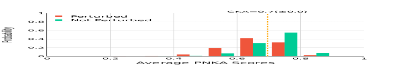
(b) R18, $p=50\%$.

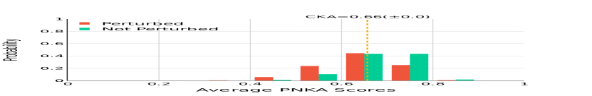
(c) R18, $p=90\%$.

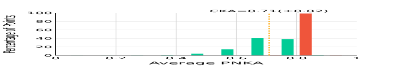
(d) VGG16, $p=10\%$.

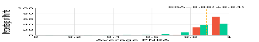
(e) VGG16, $p=50\%$.

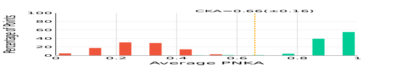
(f) VGG16, $p=90\%$.

Figure 19: Perturbed points in the test set are more likely to obtain lower similarity scores than non-perturbed (i.e. original) points for the elastic transformation. We use $p\%$ perturbed and $100-p\%$ non-perturbed points. Results are an average over 3 runs, each one containing two models trained on CIFAR-100 [25] with the same architecture but different random initialization.

C.4.3 Adversarial perturbations

CIFAR-10

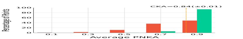
(a) R18, $p=10\%$.

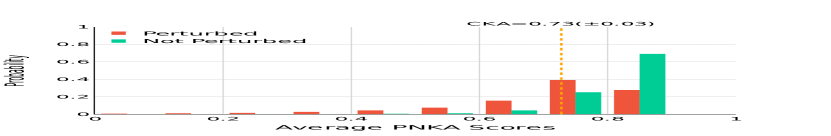
(b) R18, $p=50\%$.

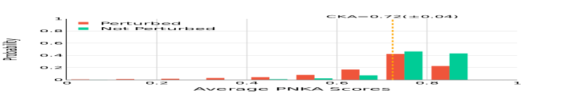
(c) R18, $p=90\%$.

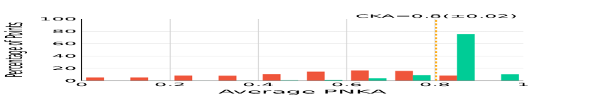
(d) VGG16, $p=10\%$.

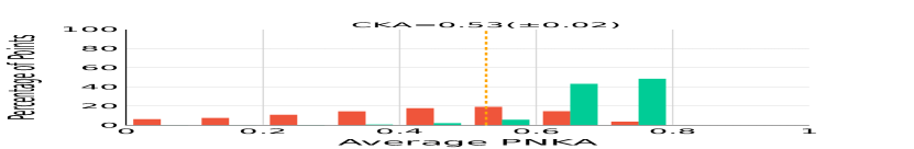
(e) VGG16, $p=50\%$.

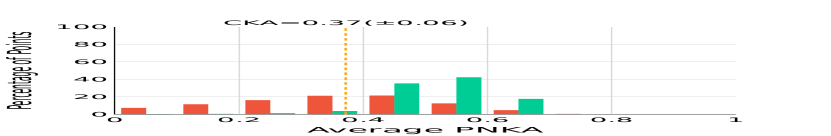
(f) VGG16, $p=90\%$.

Figure 20: Perturbed points in the test set are more likely to obtain lower similarity scores than non-perturbed (i.e. original) points for adversarial perturbation. We use $p\%$ perturbed and $100-p\%$ non-perturbed points. Results are an average over 3 runs, each one containing two models trained on CIFAR-100 [25] with the same architecture but different random initialization.

CIFAR-100

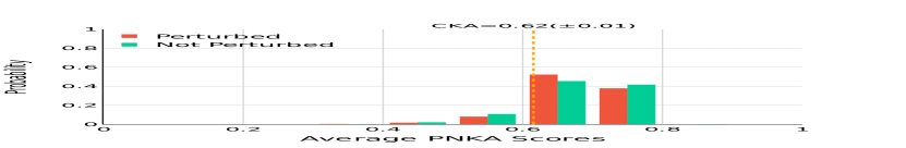
(a) R18, $p=10\%$.

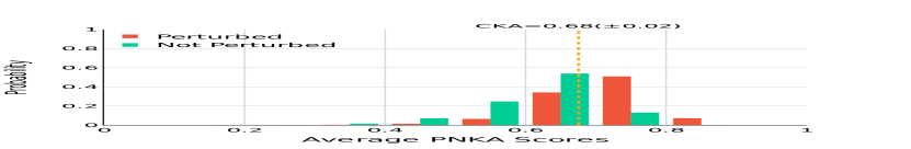
(b) R18, $p=50\%$.

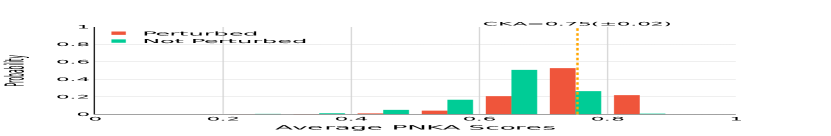
(c) R18, $p=90\%$.

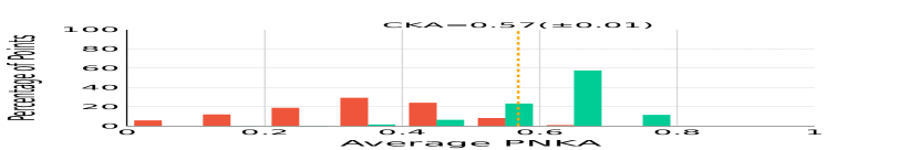
(d) VGG16, $p=10\%$.

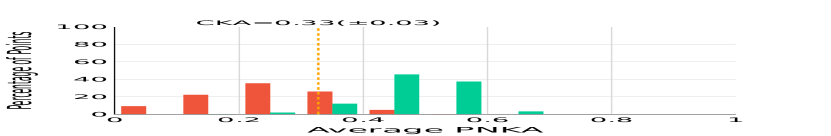
(e) VGG16, $p=50\%$.

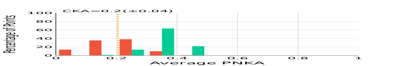
(f) VGG16, $p=90\%$.

Figure 21: Perturbed points in the test set are more likely to obtain lower similarity scores than non-perturbed (i.e. original) points for adversarial perturbation. We use $p\%$ perturbed and $100-p\%$ non-perturbed points. Results are an average over 3 runs, each one containing two models trained on CIFAR-100 [25] with the same architecture but different random initialization.

Appendix D PNKA as an Interpretability Tool

D.1 Distribution of classes for the 100 most dissimilar images when removing one neuron

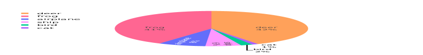
(a) Neuron 0.

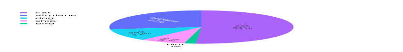
(b) Neuron 1.

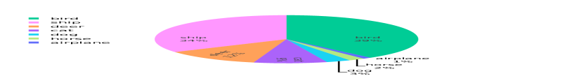
(c) Neuron 2.

(d) Neuron 3.

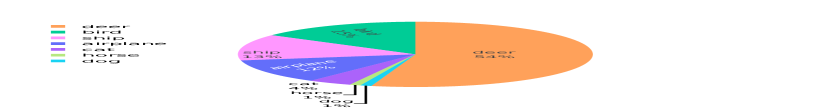
(e) Neuron 4.

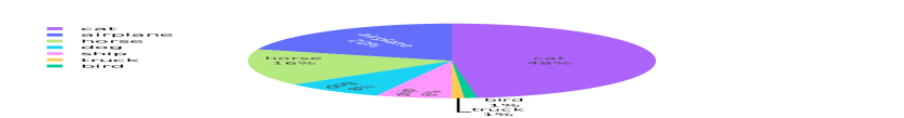
(f) Neuron 5.

(g) Neuron 6.

(h) Neuron 7.

(i) Neuron 8.

(j) Neuron 9.

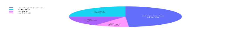
(k) Neuron 10.

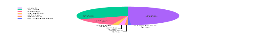
(l) Neuron 11.

(m) Neuron 12.

(n) Neuron 13.

(o) Neuron 14.

(p) Neuron 15.

(q) Neuron 16.

(r) Neuron 17.

(s) Neuron 18.

(t) Neuron 19.

(u) Neuron 20.

(v) Neuron 21.

(w) Neuron 22.

(x) Neuron 23.

Figure 22: Class distribution of the 100 images with the lowest PNKA similarity, i.e. that changes the most its representation when removing the neuron, for the penultimate layer. We show that most of the neurons capture one or two class in its majority.

D.2 Results on linear probes

		Overall	Plane	Car	Bird	Cat	Deer	Dog	Frog	Horse	Ship	Truck
Majority	#Neurons	512	49	21	53	105	91	41	38	66	20	28
>$50\%$	#Neurons	278	25	15	28	49	55	27	16	34	12	17
	Random	0.930	0.963	0.959	0.878	0.767	0.960	0.952	0.941	0.939	0.960	0.965
Accuracy on the 50 most aligned neurons (PNKA)	Plane	0.770	0.994	0.955	0.810	0.345	0.828	0.366	0.857	0.745	0.906	0.923
	Car	0.720	0.864	0.996	0.774	0.510	0.694	0.805	0.848	0.000	0.879	0.824
	Bird	0.690	0.923	0.964	0.994	0.410	0.818	0.05	0.0	0.891	0.947	0.928
	Cat	0.830	0.914	0.921	0.839	0.983	0.748	0.635	0.641	0.846	0.796	0.960
	Deer	0.87	0.852	0.990	0.853	0.691	0.997	0.772	0.891	0.844	0.942	0.876
	Dog	0.800	0.911	0.793	0.808	0.654	0.737	0.982	0.95	0.305	0.923	0.975
	Frog	0.850	0.941	0.96	0.793	0.69	0.500	0.824	0.990	0.899	0.925	0.963
	Horse	0.610	0.94	0.953	0.816	0.174	0.011	0.308	0.006	0.996	0.934	0.923
	Ship	0.860	0.805	0.907	0.903	0.549	0.881	0.818	0.909	0.870	0.991	0.940
	Truck	0.750	0.810	0.882	0.380	0.584	0.325	0.831	0.898	0.832	0.956	0.989
Accuracy on the 50 most aligned neurons (activations)	Plane	0.8	0.997	0.723	0.826	0.664	0.721	0.742	0.816	0.914	0.758	0.863
	Car	0.77	0.814	0.992	0.805	0.333	0.62	0.689	0.859	0.696	0.967	0.885
	Bird	0.73	0.94	0.919	0.991	0.793	0.654	0.205	0.853	0.128	0.851	0.916
	Cat	0.72	0.726	0.526	0.683	0.985	0.672	0.394	0.643	0.715	0.868	0.953
	Deer	0.84	0.79	0.972	0.682	0.735	0.997	0.657	0.867	0.925	0.937	0.855
	Dog	0.68	0.9	0.925	0.822	0.023	0.821	0.968	0.007	0.414	0.906	0.97
	Frog	0.8	0.942	0.722	0.137	0.746	0.851	0.895	0.993	0.86	0.933	0.92
	Horse	0.73	0.925	0.748	0.688	0.807	0.648	0.516	0.057	0.996	0.924	0.946
	Ship	0.85	0.771	0.931	0.852	0.582	0.777	0.904	0.911	0.852	0.995	0.936
	Truck	0.62	0.852	0.885	0.865	0.339	0.683	0.626	0.0	0.921	0.069	0.993
Accuracy on the 50 least aligned neurons (PNKA)	Plane	0.88	0.596	0.98	0.928	0.587	0.975	0.95	0.942	0.943	0.956	0.963
	Car	0.88	0.952	0.423	0.9	0.873	0.828	0.928	0.964	0.964	0.961	0.977
	Bird	0.83	0.918	0.978	0.018	0.834	0.97	0.933	0.921	0.805	0.95	0.971
	Cat	0.85	0.982	0.987	0.886	0.0	0.948	0.921	0.95	0.963	0.948	0.898
	Deer	0.83	0.917	0.969	0.912	0.826	0.0	0.917	0.952	0.914	0.97	0.964
	Dog	0.87	0.881	0.962	0.934	0.788	0.968	0.263	0.955	0.958	0.964	0.978
	Frog	0.84	0.946	0.979	0.926	0.832	0.922	0.915	0.0	0.915	0.971	0.95
	Horse	0.83	0.918	0.934	0.921	0.818	0.844	0.938	0.973	0.0	0.969	0.974
	Ship	0.84	0.921	0.954	0.917	0.846	0.924	0.935	0.966	0.966	0.0	0.981
	Truck	0.85	0.972	0.959	0.877	0.794	0.928	0.95	0.97	0.94	0.945	0.176
Accuracy on the 50 least aligned neurons (activations)	Plane	0.91	0.67	0.977	0.903	0.87	0.979	0.896	0.95	0.937	0.982	0.894
	Car	0.87	0.966	0.324	0.921	0.871	0.896	0.925	0.96	0.925	0.94	0.981
	Bird	0.85	0.919	0.963	0.0	0.884	0.931	0.933	0.954	0.964	0.967	0.969
	Cat	0.84	0.964	0.983	0.917	0.0	0.97	0.782	0.954	0.944	0.969	0.936
	Deer	0.84	0.88	0.956	0.872	0.913	0.0	0.91	0.945	0.946	0.981	0.964
	Dog	0.87	0.907	0.965	0.951	0.831	0.93	0.326	0.968	0.959	0.946	0.966
	Frog	0.84	0.929	0.964	0.93	0.807	0.929	0.936	0.0	0.949	0.972	0.959
	Horse	0.83	0.887	0.934	0.879	0.859	0.892	0.928	0.975	0.0	0.977	0.976
	Ship	0.84	0.959	0.96	0.911	0.781	0.93	0.936	0.962	0.971	0.02	0.974
	Truck	0.86	0.959	0.968	0.867	0.856	0.936	0.935	0.976	0.874	0.965	0.27

Table 4: Table with the results of the linear probes on 50 selected neurons. The linear probes trained on the 50 neurons that most (least) align with a specific class increase (decrease) its accuracy, compared to randomly picking 50 neurons. We also show that the results using PNKA achieves similar results with the results of using the neuron activation, which is a method specifically designed for interpretability of neurons. Due to size constraints, we altered the class names of Airplane and Automobile to Plane and Car, respectively.

Appendix E Using PNKA to analyze model interventions

E.1 Results on SemBias dataset

For each of the four word pairs $(a,b)$ in a SemBias instance, GP- and GN-Glove measure its cosine similarity with the canonical gender vector, i.e. $cos(\overrightarrow{a}-\overrightarrow{b},\overrightarrow{he}$ - $\overrightarrow{she})$. The word pair with the highest cosine similarity is selected as the “predicted” answer. If the word embeddings are correctly debiased, then the cosine similarity of the $\overrightarrow{he}$ - $\overrightarrow{she}$ vector with the gender-definition words should be high, and the similarity with the gender-stereotype words should be low, i.e. the frequency of predictions for these categories should be high and low, respectively. Table 5 depicts the results for the GN- and GP-Glove [49, 22] methods.

Embeddings	SemBias
	Definition $\uparrow$	Stereotype $\downarrow$	Neutral $\downarrow$
GloVe	80.2	10.9	8.9
GN-GloVe	97.7	1.4	0.9
GP-GloVe	84.3	8.0	7.7
GP-GN-GloVe	98.4	1.1	0.5

Table 5: Frequency of predictions for gender relational analogies [22]. Each column shows the frequency with which the respective word-pair category (gender-definitional, gender-stereotype, gender-neutral) is predicted as having the highest cosine similarity with the canonical gender vector $\overrightarrow{he}$ - $\overrightarrow{she}$. The more often gender-definition words are predicted as being most gender-aligned, as opposed to gender-stereotype words, the less biased an embedding approach can be considered.

E.2 Additional information on analyzing gender changes

The similarity scores from PNKA in Figure 4 (main paper) show that across all three methods, the words whose embeddings change the most are the gender-definition words. This observation, however, is not consistent with the expectation that the embeddings that should change the most are the gender-stereotypical ones, not the gender-definitional ones. The fact that the classification results for word pairs in SemBias nonetheless behave as expected suggests the hypothesis that instead of removing gender information from the gender-stereotypical word pairs, the debiasing methods might instead be amplifying the gender information in the gender-definition word pairs.

Thus, to test this hypothesis, for each embedding approach $\phi_{e}$ and word $i$, we project the corresponding word embeddings $w_{i}^{(e)}=\phi_{e}(i)$ into the gender vector direction $g^{(e)}=\overrightarrow{he^{(e)}}$ - $\overrightarrow{she^{(e)}}$ and compute the projection magnitudes $p_{i}^{(e)}=~{}\rVert g^{(e)\top}w_{i}^{(e)}\rVert_{2}$. The higher $p_{i}^{(e)}$ is, the more gender information is contained in the word embedding vector $w_{i}^{(e)}$. To understand how much each of the debiased embedding methods $\phi_{e}$ change the amount of gender information, relative to the original GloVe embeddings, we analyze the percentage difference in magnitude, defined as

$$\omega_{i}^{(e)}=\frac{p_{i}^{(e)}-p_{i}^{(glove)}}{p_{i}^{(glove)}}$$

$\omega_{i}^{(e)}=0$ indicates that the gender information in the debiased embedding has not changed relative to GloVe, while $\omega_{i}^{(e)}>0$ (or $\omega_{i}^{(e)}<0$) indicates an increase in the gender information associated with $i$.

E.3 Cosine similarity does not provide the same insight

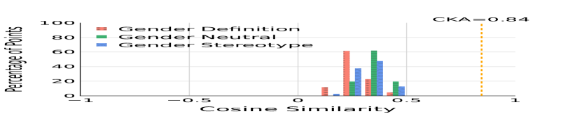
(a) GloVe $\times$ GN-GloVe.

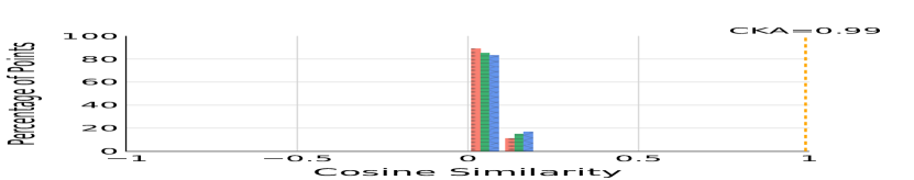
(b) GloVe $\times$ GP-GloVe.

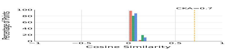
(c) GloVe $\times$ GP-GN-GloVe.

Figure 23: Cosine similarity does not provide the same insight as PNKA. Instead, for cosine similarity, most of the words’ embeddings change substantially from GloVe (baseline) to its debiased versions, i.e. cosine similarity is mostly between 0 and 0.5 for all group of words.

References

- [1] Guillaume Alain and Yoshua Bengio. Understanding intermediate layers using linear classifier probes. arXiv preprint arXiv:1610.01644, 2016.
- [2] Julia Angwin, Jeff Larson, Surya Mattu, and Lauren Kirchner. Machine bias. In Ethics of data and analytics, pages 254–264. Auerbach Publications, 2016.
- [3] Anish Athalye, Logan Engstrom, Andrew Ilyas, and Kevin Kwok. Synthesizing robust adversarial examples. In International conference on machine learning, pages 284–293. PMLR, 2018.
- [4] Christina Baek, Yiding Jiang, Aditi Raghunathan, and J Zico Kolter. Agreement-on-the-line: Predicting the performance of neural networks under distribution shift. Advances in Neural Information Processing Systems, 35:19274–19289, 2022.
- [5] David Bau, Bolei Zhou, Aditya Khosla, Aude Oliva, and Antonio Torralba. Network dissection: Quantifying interpretability of deep visual representations. In Proceedings of the IEEE conference on computer vision and pattern recognition, pages 6541–6549, 2017.
- [6] Tolga Bolukbasi, Kai-Wei Chang, James Y Zou, Venkatesh Saligrama, and Adam T Kalai. Man is to computer programmer as woman is to homemaker? debiasing word embeddings. Advances in neural information processing systems, 29, 2016.
- [7] Nick Cammarata, Gabriel Goh, Shan Carter, Ludwig Schubert, Michael Petrov, and Chris Olah. Curve detectors. Distill, 5(6):e00024–003, 2020.
- [8] Ting Chen, Simon Kornblith, Mohammad Norouzi, and Geoffrey Hinton. A simple framework for contrastive learning of visual representations. arXiv preprint arXiv:2002.05709, 2020.
- [9] Elliot Creager, David Madras, Jörn-Henrik Jacobsen, Marissa Weis, Kevin Swersky, Toniann Pitassi, and Richard Zemel. Flexibly fair representation learning by disentanglement. In International conference on machine learning, pages 1436–1445. PMLR, 2019.
- [10] MohammadReza Davari, Nader Asadi, Sudhir Mudur, Rahaf Aljundi, and Eugene Belilovsky. Probing representation forgetting in supervised and unsupervised continual learning. In Proceedings of the IEEE/CVF Conference on Computer Vision and Pattern Recognition, pages 16712–16721, 2022.
- [11] MohammadReza Davari, Stefan Horoi, Amine Natik, Guillaume Lajoie, Guy Wolf, and Eugene Belilovsky. Reliability of cka as a similarity measure in deep learning. In International Conference on Learning Representations, 2023.
- [12] Jacob Devlin, Ming-Wei Chang, Kenton Lee, and Kristina Toutanova. Bert: Pre-training of deep bidirectional transformers for language understanding. arXiv preprint arXiv:1810.04805, 2018.
- [13] Frances Ding, Jean-Stanislas Denain, and Jacob Steinhardt. Grounding representation similarity through statistical testing. Advances in Neural Information Processing Systems, 34:1556–1568, 2021.
- [14] Saurabh Garg, Sivaraman Balakrishnan, Zachary C Lipton, Behnam Neyshabur, and Hanie Sedghi. Leveraging unlabeled data to predict out-of-distribution performance. arXiv preprint arXiv:2201.04234, 2022.
- [15] Robert Geirhos, Carlos R. M. Temme, Jonas Rauber, Heiko H. Schütt, Matthias Bethge, and Felix A. Wichmann. Generalisation in humans and deep neural networks. In S. Bengio, H. Wallach, H. Larochelle, K. Grauman, N. Cesa-Bianchi, and R. Garnett, editors, Advances in Neural Information Processing Systems, volume 31. Curran Associates, Inc., 2018.
- [16] Hila Gonen and Yoav Goldberg. Lipstick on a pig: Debiasing methods cover up systematic gender biases in word embeddings but do not remove them. In Proceedings of NAACL-HLT, pages 609––614, 2019.
- [17] Jean-Bastien Grill, Florian Strub, Florent Altché, Corentin Tallec, Pierre Richemond, Elena Buchatskaya, Carl Doersch, Bernardo Avila Pires, Zhaohan Guo, Mohammad Gheshlaghi Azar, et al. Bootstrap your own latent-a new approach to self-supervised learning. Advances in neural information processing systems, 33:21271–21284, 2020.
- [18] William L Hamilton, Jure Leskovec, and Dan Jurafsky. Cultural shift or linguistic drift? comparing two computational measures of semantic change. In Proceedings of the conference on empirical methods in natural language processing. Conference on empirical methods in natural language processing, volume 2016, page 2116. NIH Public Access, 2016.
- [19] Kaiming He, Xiangyu Zhang, Shaoqing Ren, and Jian Sun. Deep residual learning for image recognition. In Proceedings of the IEEE conference on computer vision and pattern recognition, pages 770–778, 2016.
- [20] Dan Hendrycks and Thomas Dietterich. Benchmarking neural network robustness to common corruptions and perturbations. In International Conference on Learning Representations, 2019.
- [21] Yiding Jiang, Vaishnavh Nagarajan, Christina Baek, and J Zico Kolter. Assessing generalization of sgd via disagreement. arXiv preprint arXiv:2106.13799, 2021.
- [22] Masahiro Kaneko and Danushka Bollegala. Gender-preserving debiasing for pre-trained word embeddings. In Proceedings of the 57th Annual Meeting of the Association for Computational Linguistics, pages 1641––1650, 2019.
- [23] Simon Kornblith, Mohammad Norouzi, Honglak Lee, and Geoffrey Hinton. Similarity of neural network representations revisited. In International Conference on Machine Learning, pages 3519–3529. PMLR, 2019.
- [24] Nikolaus Kriegeskorte, Marieke Mur, and Peter A Bandettini. Representational similarity analysis-connecting the branches of systems neuroscience. Frontiers in systems neuroscience, page 4, 2008.
- [25] Alex Krizhevsky, Geoffrey Hinton, et al. Learning multiple layers of features from tiny images. 2009.
- [26] Aarre Laakso and Garrison Cottrell. Content and cluster analysis: assessing representational similarity in neural systems. Philosophical psychology, 13(1):47–76, 2000.
- [27] Yann LeCun, Ido Kanter, and Sara Solla. Second order properties of error surfaces: Learning time and generalization. Advances in neural information processing systems, 3, 1990.
- [28] Yixuan Li, Jason Yosinski, Jeff Clune, Hod Lipson, and John Hopcroft. Convergent learning: Do different neural networks learn the same representations? arXiv preprint arXiv:1511.07543, 2015.
- [29] Weiyang Liu, Rongmei Lin, Zhen Liu, James M Rehg, Liam Paull, Li Xiong, Le Song, and Adrian Weller. Orthogonal over-parameterized training. In Proceedings of the IEEE/CVF Conference on Computer Vision and Pattern Recognition, pages 7251–7260, 2021.
- [30] Christos Louizos, Kevin Swersky, Yujia Li, Max Welling, and Richard Zemel. The variational fair autoencoder. arXiv preprint arXiv:1511.00830, 2015.
- [31] Seyed-Mohsen Moosavi-Dezfooli, Alhussein Fawzi, Omar Fawzi, and Pascal Frossard. Universal adversarial perturbations. In Proceedings of the IEEE conference on computer vision and pattern recognition, pages 1765–1773, 2017.
- [32] Ari Morcos, Maithra Raghu, and Samy Bengio. Insights on representational similarity in neural networks with canonical correlation. Advances in Neural Information Processing Systems, 31, 2018.
- [33] Vedant Nanda, Till Speicher, Camila Kolling, John P Dickerson, Krishna Gummadi, and Adrian Weller. Measuring representational robustness of neural networks through shared invariances. In International Conference on Machine Learning, pages 16368–16382. PMLR, 2022.
- [34] Thao Nguyen, Maithra Raghu, and Simon Kornblith. Do wide and deep networks learn the same things? uncovering how neural network representations vary with width and depth. In International Conference on Learning Representations, 2021.
- [35] Thao Nguyen, Maithra Raghu, and Simon Kornblith. On the origins of the block structure phenomenon in neural network representations. 2021.
- [36] Cathy O’neil. Weapons of math destruction: How big data increases inequality and threatens democracy. Crown, 2017.
- [37] Nicolas Papernot, Patrick McDaniel, Somesh Jha, Matt Fredrikson, Z Berkay Celik, and Ananthram Swami. The limitations of deep learning in adversarial settings. In 2016 IEEE European symposium on security and privacy (EuroS&P), pages 372–387. IEEE, 2016.
- [38] Alec Radford, Jong Wook Kim, Chris Hallacy, Aditya Ramesh, Gabriel Goh, Sandhini Agarwal, Girish Sastry, Amanda Askell, Pamela Mishkin, Jack Clark, et al. Learning transferable visual models from natural language supervision. In International conference on machine learning, pages 8748–8763. PMLR, 2021.
- [39] Aniruddh Raghu, Maithra Raghu, Samy Bengio, and Oriol Vinyals. Rapid learning or feature reuse? towards understanding the effectiveness of maml. arXiv preprint arXiv:1909.09157, 2019.
- [40] Maithra Raghu, Justin Gilmer, Jason Yosinski, and Jascha Sohl-Dickstein. Svcca: Singular vector canonical correlation analysis for deep learning dynamics and interpretability. Advances in neural information processing systems, 30, 2017.
- [41] Maithra Raghu, Thomas Unterthiner, Simon Kornblith, Chiyuan Zhang, and Alexey Dosovitskiy. Do vision transformers see like convolutional neural networks? Advances in Neural Information Processing Systems, 34:12116–12128, 2021.
- [42] Vinay V Ramasesh, Ethan Dyer, and Maithra Raghu. Anatomy of catastrophic forgetting: Hidden representations and task semantics. arXiv preprint arXiv:2007.07400, 2020.
- [43] Christian Szegedy, Wojciech Zaremba, Ilya Sutskever, Joan Bruna, Dumitru Erhan, Ian Goodfellow, and Rob Fergus. Intriguing properties of neural networks. arXiv preprint arXiv:1312.6199, 2013.
- [44] Rohan Taori, Achal Dave, Vaishaal Shankar, Nicholas Carlini, Benjamin Recht, and Ludwig Schmidt. Measuring robustness to natural distribution shifts in image classification. In Advances in Neural Information Processing Systems, 2020.
- [45] Chenxu Wang, Wei Rao, Wenna Guo, Pinghui Wang, Jun Liu, and Xiaohong Guan. Towards understanding the instability of network embedding. IEEE Transactions on Knowledge and Data Engineering, 34(2):927–941, 2020.
- [46] Liwei Wang, Lunjia Hu, Jiayuan Gu, Zhiqiang Hu, Yue Wu, Kun He, and John Hopcroft. Towards understanding learning representations: To what extent do different neural networks learn the same representation. Advances in neural information processing systems, 31, 2018.
- [47] Di Xie, Jiang Xiong, and Shiliang Pu. All you need is beyond a good init: Exploring better solution for training extremely deep convolutional neural networks with orthonormality and modulation. In Proceedings of the IEEE Conference on Computer Vision and Pattern Recognition, pages 6176–6185, 2017.
- [48] Rich Zemel, Yu Wu, Kevin Swersky, Toni Pitassi, and Cynthia Dwork. Learning fair representations. In International conference on machine learning, pages 325–333. PMLR, 2013.
- [49] Jieyu Zhao, Yichao Zhou, Zeyu Li, Wei Wang, and Kai-Wei Chang. Learning gender-neutral word embeddings. In Conference on Empirical Methods in Natural Language Processing, pages 4847–4853, 2018.