Global Layers: Non-IID Tabular Federated Learning

Abstract

Data heterogeneity between clients remains a key challenge in Federated Learning (FL), particularly in the case of tabular data. This work presents Global Layers (GL), a novel partial model personalization method robust in the presence of joint distribution $P(X,Y)$ shift and mixed input/output spaces $X\times Y$ across clients. To the best of our knowledge, GL is the first method capable of supporting both client-exclusive features and classes. We introduce two new benchmark experiments for tabular FL naturally partitioned from existing real world datasets: i) UCI Covertype split into 4 clients by "wilderness area" feature, and ii) UCI Heart Disease, SAHeart, UCI Heart Failure, each as clients. Empirical results in these experiments in the full-participant setting show that GL achieves better outcomes than Federated Averaging (FedAvg) and local-only training, with some clients even performing better than their centralized baseline.

1 Introduction

Federated Learning (FL) is an emerging framework for collaboratively training machine learning models across distributed private datasets, termed clients. First proposed as a way to efficiently train language models over large numbers of edge devices [1], FL has been since recognized more generally as a privacy-preserving alternative to centralized learning [2]. This has attracted recent interest in enterprise applications, as centralizing data may be prohibited by regulation or may have unwanted business impact such as trade secret disclosure.

A prominent scenario is training diagnostic models across hospitals [3, 4, 5]. A hospital may have insufficient data to train a high quality model alone. FL enables model training while data remains at source. When the assumption that the $K$ clients are independent and identically distributed (IID) samples from a single meta-distribution is satisfied, i.e. $k\overset{iid}{\sim}P(X,Y|k)\,\forall k\in K$, we can expect the resulting federated model to converge with performance comparable to a centralized model [6].

Unfortunately, this assumption is rarely met in practice. Geographically distributed data sources will inherently reflect their distributional biases. Consider that hospitals may address disparate patient demographics $P(X)$ with distinct disease susceptibilities $P(X|Y)$, treatment responses $P(Y|X)$, and outcomes $P(Y)$ [7, 8, 9]. Distribution shift among clients causes their local gradient estimates to drift [10] resulting in reduced or stalled global model convergence [6, 11, 12, 13, 14]. Moreover, hospitals may maintain different medical record fields for their $X$ and $Y$ due to varying interventions, testing equipment, encoding choices, and regulatory requirements. Yet, heterogeneous input/output spaces are incompatible with full-parameter federated models.

Many early FL works tried to avoid the non-IID issue entirely by focusing on special cases. Horizontal FL methods assume the existence of a sufficiently explanatory in-distribution subset of "common grounds" features and consistent target spaces [2]. Vertical FL methods support heterogeneous features spaces but assume a sufficiently large alignment in sample space [15]. Existing transfer FL methods support missing features and labels among clients and assume overlapping sample and feature space. In all three cases, conditional distribution shift and target space inconsistency remain as challenges, and we lose all client specific information that could have been beneficial for learning. None of these settings can address our hospital scenario, and others scenarios that place no assumptions of overlapping feature or samples and where the joint distribution $P(X,Y)$ and spaces $X\times Y$ may arbitrarily differ across clients $k\in K$.

To the best of our knowledge, no method so far supports simultaneous feature and label space heterogeneity across clients without assumptions of overlapping features, labels, or samples. We could only find two works that propose and study methods supporting disjoint features but not labels [16, 17] and vice-versa [18, 19]. Second, while tabular data format is the most common in business [20], the majority of works study only image and text datasets. These already have a natural shared representation space across tasks e.g. pixels and token sequences, often also preserving their labels, with a rich spatial or temporal structure, unlike tabular data, which contains arbitrarily ordered ordinal and numeric features.

In this work, we propose Global Layers (GL), a novel partial model personalization framework capable of addressing the most general case of statistical heterogeneity in FL. GL strongly separates private client input/output layers and global inner federated layers with the goal of learning personalized compositions of global equipredictive transformations. GL places no restriction on the term that varies in the joint distribution $P(X,Y)$ across clients and makes no assumptions of overlap or specific ordering in either the features, targets or samples across clients.

To empirically analyze GL and given a lack of existing real-world non-IID tabular FL benchmark experiments appropriate for our setting, we introduce two new experiments constructed from existing real-world public datasets with natural data partitions: i) UCI Covertype split by "wilderness area" feature into 4 regionally-distributed, single-source clients, and ii) 3 independent heart disease classification datasets with each as a client: UCI Heart Disease, SAHeart, and UCI Heart Failure, collected from hospitals in USA, South Africa, and Pakistan, respectively.

Our results in both experiments in the full-participant setting show that GL achieves better outcomes than both full-parameter aggregation with Federated Averaging (FedAvg) and local-only training, with some clients even performing better than their centralized baseline.

2 Background and Related Work

2.1 Federated Learning

The standard FL objective is one global model $w\in\mathbb{R}^{d}$ that minimizes the aggregated local losses:

$$\underset{w}{\min}\;F(w):=\mathbb{E}_{k}[F_{k}(w)]=\sum_{k}^{K}{\alpha_{k}F_{k}(w)}$$ (1)

Where the loss for client $k\in K$ with private labeled data $z_{k}=(x_{k},y_{k})$ is:

$$F_{k}(w)=\mathbb{E}_{z_{k}\sim P_{k}}[f_{k}(w)]=\frac{1}{n_{k}}\sum_{i=1}^{n_{k}}f_{k}(w,z_{k,i})$$ (2)

FedAvg [1] takes a weighted average for $a_{k}$, where $n_{k}$ is the number of samples in the $k$th client:

$$\alpha_{k}=\frac{n_{k}}{\sum_{k}^{K}{n_{k}}}$$ (3)

Implicit in this form is the assumption of an aggregated target distribution [21]:

$$P=\sum_{k}^{K}\alpha_{k}P_{k}$$ (4)

For a moment let us set aside the dimensionality implications of using the same $w$ for all clients. The assumption in 4 illustrates why full-parameter federation with a single global model $w$ struggles in the presence of distribution shift, and in particular concept drift, among clients. A single global model effectively interpolates between client distributions, giving each client the same averaged prediction for a particular input. While we are instead interested in a model that extrapolates beyond client distributions and with client-appropriate predictions.

Consider a toy example of 2 clients $i,j$ performing binary classification where one conditional probability distribution is the compliment of the other, i.e. $P_{i}=1-P_{j}$. From 4 we see the learning objective becomes a uniform distribution. A single global model will give predictions that are wrong for both clients, and will not converge as its gradients updates will tend to cancel out.

This limitation is applicable to any non-IID FL method relying on the "one model fits all" assumption [21, 22, 23]. For example, methods that attempt to address distribution shift through improvements in the optimization [10, 13, 21, 24, 25, 26, 27, 28, 29] can help with covariate and prior probability shift but they alone cannot address concept shift or concept drift.

2.2 Personalized Federated Learning

Full-model personalization

These methods address concept shift and concept drift by permitting local model divergence from the global model $w$. While the assumption of consistent input/output dimensionality remains, we again set this aside for a moment and focus only on distribution shift.

Fine-tuning [30, 31, 22] can help with concept shift and concept drift [2] but fine-tuned models are vulnerable to local silo [32] or global model [33] drift, and can over-fit, corrupt global information, and struggle to generalize OOD [34]. Pre-training [35] faces similar issues. Some works [36, 37, 38, 39, 40] have explored meta-learning to optimize for a well-initialized global model that best optimizes during local fine-tuning, observing improvement on these issues. Though, these methods must calculate the Hessian, an expensive step, or approximate it with a performance loss [41].

While fine-tuning methods operate in distinct phases, proximal operator methods [41, 42, 43, 44, 45, 46, 47, 48, 49] simultaneously train separate local-only and global parameters with a proximal penalty as a selective multi-task transfer learning mechanism. These generally extend 1 with penalty $R_{k}$, where $\Omega$ often contains some relevant global information, and $R_{k}=\frac{\lambda}{2}{|w_{k}-w|}^{2}$ is a common choice to penalize parameter divergence between local and global models.

$$\underset{w,\{w_{k}\}_{k=1}^{K}}{\min}\;\sum_{k}^{K}{\alpha_{k}\left(F_{k}(w_{k})+R_{k}(w_{k},\Omega)\right)}$$ (5)

Related are interpolation methods that learn client-specific mixtures of local and global models, often also using a proximal penalty [50, 51] or a different mechanism [22, 52, 53, 54, 55, 56, 57].

Despite increased non-IID robustness over FedAvg in empirical and theoretical analyses, both proximal and interpolation methods restrict the extent that local models can drift from the global model, ultimately limiting local convergence potential and thus the extent of distribution shift they can address [45]. Consider the toy example from earlier; these methods would still be unable to address this case. Though some works explore penalties $R_{k}$ independent of a global $w$, for example aligning on local model output divergence [18, 58, 59], we lose any transfer learning benefits we could have otherwise obtained in the presence of distribution shift. In general, designing $R_{k}$ is non-trivial as task relationships may not be well specified, particularly within latent space.

Partial-model personalization

The methods we described for full-model personalization can all be extended to work with restricted parameters, for example fine-tuning [60], meta-learning [40], and proximal methods [5, 61]. A general form is that $w_{k}=(u,v_{k})$ is the full model with global $u$ and local $v_{k}$ components and 1 extends to:

$$\underset{w,\{w_{k}\}_{k=1}^{K}}{\min}\;\sum_{k}^{K}{\alpha_{k}F_{k}(w_{k})}$$ (6)

While federating a subset of parameters allows for flexibility in input/output dimensionality and capacity in the other private parameters $v_{k}$, we mentioned earlier that only recently have a handful of works begun to analyze cases of non-overlapping features [16, 17], and labels [18, 19], but not yet both. Other works so far have assumed consistent feature and label spaces and restricted their focus on distribution shift. For example, LG-FedAvg [62] proposed personalized base layers to extract invariant representations, yet studies only covariate shift caused by 90 degree image rotations. Similarly, FedPer [63] and other works [9, 59, 64, 65] propose a global base with personalized heads but again make specific assumptions of distribution consistency and focus on image and text. A few works have combined other methods with personalized layers such as partial meta-learning in PMFL [40], proximal methods [5, 61], and more [66, 67].

2.3 Out-Of-Distribution Learning

Learning in the presence of distribution shift has an extensive history of study in the centralized setting [68, 69, 70, 71], where the out-of-distribution (OOD) problem refers to training a predictor on limited coverage training supports that can generalize over unobserved test distributions [72]. Remaining consistent with notation used in OOD literature, a common treatment [73] is that there exists a potentially unknown environmental variable $e\in\mathcal{E}$ conditioning datasets sampled from a meta-distribution $P(X,Y|e)=P(X|e)P(Y|X,e)$ where $\mathcal{E}_{train}\subseteq\mathcal{E}$ is the training data which can be multi-source and $Supp(\mathcal{E})$ is the space of all possible test environments. This is a problematic scenario for Empirical Risk Minimization [74] (ERM) whose asymptotically optimal learning principle depends on sufficient in-distribution training coverage.

A recent line of works [71, 72, 73, 75, 76, 77] have proposed alternatives to ERM that attempt to learn invariant predictors that are able to generalize OOD while ignoring spurious correlations. The key idea in all these works is that learning an equipredictive representation $\varphi(X)$ promotes learning invariant relationships across environments, described as $P(Y|\varphi(X),e)\,\forall e\in\mathcal{E}$.

A few recent works have explored applying these ideas to the FL setting [65, 78, 79, 80] but have focused the scenario of generalizing from $k\in K$ training clients to a new unseen $k+1$ client.

3 Global Layers (GL)

3.1 Methodology

In this work we focus only on the full-participant setting and the generalization performance on each client’s own cross-validation test set. We extend the standard FL formulation to capture the type of data heterogeneity we mentioned earlier and that we present in our empirical analyses.

Each client dataset $D_{k}=\{(x_{k,1},y_{k,1})...(x_{k,n_{k}},y_{k,n_{k}})\}\in(X_{k},Y_{k})^{n_{k}}$ of size $n_{k}$ has a possibly disjoint feature space $X_{k}\in\mathbb{R}^{d_{k}}$ and target space $Y_{k}\in\mathbb{R}^{c_{k}}$, where $d_{k}$ is the number of local features, and $c_{k}$ is the number of local classes, with $c=1$ for regression. Client datasets are IID samples $D_{k}\overset{iid}{\sim}P_{k}(X_{k},Y_{k})$ from different meta-distributions $P_{k}\overset{non-iid}{\sim}P(X,Y|k)\,\forall k\in K$.

While our contribution does not require overlapping features, targets or samples, which is our goal, any existence of these would improve learning outcomes. In practical terms, it would make sense for clients to have something in common, otherwise the reason for training together is unclear.

The key idea in our work is that rather than try to learn invariant relationships between client features and targets, which does not have clear definition when feature and target spaces are disjoint, is to instead try to learn invariant relationships within inner layer latent-space transformations across clients $P(Z_{L}|\varphi(Z_{L-1}),k)\,\forall k\in K$. In particular, we want to learn these as personalized compositions with client specific dynamics. The intuition is that despite distinct input/output spaces, we still wish to preserve shared invariant transformations. At the same time, we do not want to restrict to the case where these relationships such as conditional distribution are fully preserved across clients.

3.2 Learning Objective

Inspired by the recent OOD literature, we propose learning a global equipredictive $\omega:H\rightarrow\hat{H}$ such that: $P(Y_{k}|v_{k}(\omega(u_{k}(X_{k})))\,\forall k\in K$, where $u_{k}:X_{k}\rightarrow H$ and $v_{k}:\hat{H}\rightarrow\hat{Y}_{k}$ are client specific input and output transformations, respectively. We extend 6 with $w_{k}=\{u_{k},\omega,v_{k}\}$.

$$\underset{w,\{u_{k},v_{k}\}_{k=1}^{K}}{\min}\;F(u_{k},\omega,v_{k}):=\sum_{k}^{K}{F_{k}(u_{k},\omega,v_{k})}$$ (7)

Note that $a_{k}=1$ as we ensure consistent local gradient updates, elaborated in Section 3.4.

The empirical loss at private sample $z_{k,i}\overset{iid}{\sim}P(X_{k},Y_{k})$ for the $k$th client is therefore:

$$f_{k,z_{k,i}}(w_{k})$$ (8)

Optimizing 7 can be done following standard horizontal FL practices, including combining this objective with other personalization methods such as adding a proximal penalty term.

3.3 Model Architecture

The learning objective we just provided is architecturally agnostic, requiring only that $w_{k}$ can be composed into a feedforward model $f_{k}$ for each client that supports its local input/output dimensionality. Generally the dimensionality, number of instances and task complexity will vary between clients which can motivate different capacities in private components. Though we did explore this, in our experiments we found that consistent architectures across clients works well. This leaves us with three main design choices for our overall model architecture: the choice of input layers $u$, output layers $v$ and inner global layers $\omega$. We show this in Figure 1.

In this work we only explored neural-network architectures for each, though in theory this is not a constraint. Neural-networks have a well-studied ability to compose abstract and complex hierarchical features that can transfer across latent spaces [81], even in the tabular domain [82].

Recently some works have proposed Transformer [83] based models for the tabular domain, such as TabTransformer [44] and other similar architectures [84, 85, 86, 87, 88] to capture high-order feature interactions across different subspaces, scales and even samples. Such models have demonstrated to be competitive with even Gradient Decision Boosted Tree (GDBT) ensembles [84, 89] which was previously undisputed in its performance with tabular data.

In both of our experiments we use a TabTransformer inspired architecture with 6 stacked Transformer layers followed by a partially federated Multi-Layer Perceptron (MLP), shown in Figures 2 and 3.

We first Batch Normalize [90], then pass all client features, including ordinal and numerical, through a private Entity Embedding-like [91] layer. Specifically, all features $x_{k}:=\{x_{k,1},...,x_{k,d_{k}}\}$ receive their own fully-connected linear dense representation $\mathbf{e}$ parameterized by $\phi_{k}$:

$$\mathbf{E}(x_{k}):=\{\mathbf{e}_{{\phi}_{k,1}}(x_{k,1}),...,\mathbf{e}_{{\phi}_{k,d_{k}}}(x_{k,d_{k}})\}$$ (9)

A dense layer per feature eliminates token conflicts. In particular this is a mechanism for the model to learn to transform features independently to best embed local activations into the global latent space to mitigate both covariate shift and concept shift. Intuitively, dissimilar embeddings can be encouraged to be similar when they share conditional likelihoods, and vice-versa.

Next are the 6 Transformer layers, after which we flatten and pass through the MLP. The MLP is 5 feedforward layers alternating between a) a fully-connected layer with batchnorm, Scaled Exponential Linear Unit [92] (SELU) activation and dropout, and b) a similar fully-connected layer but with self-gating and a residual skip connection. Only the second, third, and fourth MLP layers are federated, allowing for heterogeneous input/output dimensionality. Decoupling client output layers also allows client models to mitigate concept drift.

See Appendix C for much more details.

3.4 Training Algorithm

Our proposed training algorithm BatchAlignedFedAvg is based on standard FedAvg with two differences. The first difference is that rather than specifying a batch size, instead we specify a total number of batches for each local epoch as a hyperparameter, which all clients use, giving us a consistent number of local gradient updates before the aggregation step and allowing us to set $a_{k}=1$. This ensures each client contribution to the global update is proportional to its local empirical loss only, rather than the quantity of instances. This also avoids local under or oversampling which can distort client distribution, particularly when sample sizes are low or imbalanced between clients. The second difference is aggregation is done each time all clients complete a local pass on their batch.

Although in Algorithm 1 we show a local training step in the form of an SGD update, any optimizer can work, such as AdamW [93].

Input : Initialized $\omega^{(0)}$, $\{u_{k}^{(0)},v_{k}^{(0)}\}_{k=1}^{K}$, number of rounds $T$, clients $K$, learning rate $\gamma$, number of batches $B_{n}$, loss functions $F_{k}$ and global layer update rate $\eta$

for $t=0,1,...,T-1$ do

       Server broadcasts global layers $\omega^{(t)}$ to all clients

       for $b=0,1,...,B_{n}-1$ do

             for clients $k\in K$ in parallel do

                   client trains locally

                   $\{u_{k},\omega_{k},v_{k}\}^{(t+1)}=\{u_{k},\omega_{k},v_{k}\}^{(t)}-\gamma\hat{\nabla}F_{k}(u_{k}^{(t)},\omega_{k}^{(t)},v_{k}^{(t)})$

                   client sends updated global layers $\omega_{k}^{(t+1)}$ back to server

             end for

            server aggregates all global layers $\omega^{(t+1)}=\sum_{k}^{K}\omega_{k}^{(t+1)}$

             for clients $k\in K$ in parallel do

                   client updates its global layers $\omega_{k}^{(t+1)}=\eta\omega_{k}^{(t+1)}+(1-\eta)\omega^{(t+1)}$

             end for

            

       end for

      

end for

Algorithm 1 BatchAlignedFedAvg

4 Experiments

We now describe the experiments we conducted to obtain the empirical results that justify our proposed method.

4.1 Experiment Settings

We could not find existing suitable FL benchmark datasets that contained mixed input/output spaces, as such cases have only recently been motivated in non-IID FL settings. We were cautious and chose to avoid randomly partitioning existing centralized benchmarks dataset, as extracting random subsets does not change the conditional distribution much, and conditioning on arbitrary attributes can introduce spurious correlations and destroy any existing real-world invariant relationships [71]. Instead we took two approaches to construct realistic experiments with natural heterogeneity from existing public benchmark datasets. These are shown in Table 1, with original sources in Table 13.

In the first case we undid the multi-source centralization that was done in the Covertype dataset by separating 4 clients based on their "wilderness area" ordinal attribute. This geographically locates each client to a slightly different region within Roosevelt National Forest of northern Colorado, with different elevations, species, and other local ecological attributes. Each client has a different set of soil type classes, though incidentally there is some overlap.

In the second case we took 3 different datasets that classify heart disease: a) UCI Heart Disease [94] in the Cleveland, USA setting, b) South Africa Heart Disease [95], and c) UCI Heart Failure from Faisalabad, Pakistan [96]. These represent independent diagnostic factors leading to shared binary outcomes: no-presence or presence. The feature spaces across these datasets are disjoint.

Both experiments use the same model with the only difference being larger embedding sizes for the larger Covertype datasets. Models are randomly initialized with consistent random seeds across clients.

A fully detailed account on the construction of both experiments is provided in Appendix D.

4.2 Baseline Methods

In order to compare our numerical results obtained with GL we consider three baseline methods.

1. FedAvg denotes a single global model $w$ where all parameters are aggregated during federation. As this is inconsistent with feature and target space differences across clients, we take the strategy of padding inconsistent dimensionality with 0’s i.e. missing values, so that the spaces do align. We explain this more in the Appendix.

2. Local denotes no federated aggregation done at all. In this case clients do separate local-only training over their private data.

3. Centralized denotes breaking privacy and combining all data into a single centralized dataset.

Experiment	Dataset	Features	Classes	Train	Test	Validation	Total
Covertype	Comanche	11	6	4772	247015	1578	253365
	Neota	11	3	385	29385	114	29884
	Poudre	11	4	3509	32293	1167	36969
	Rawah	11	4	2675	257199	922	260796
	Centralized	11	6	11340	565892	3780	581012
Heart Disease	Cleveland	13	2	182	100	21	304
	South Africa	9	2	278	153	31	462
	Faisalabad	12	2	180	100	20	299

Table 1: Summary of experiments and tabular datasets used

		AUROC (%)			(Balanced) Accuracy1 (%)
Experiment	Dataset	Local	FedAvg	GL	Local	FedAvg	GL
Covertype	Comanche	$88.29$	$79.58$	$\mathbf{92.09}$	$80.82$	$80.46$	$\mathbf{83.81}$
	Neota	$79.44$	$60.92$	$\mathbf{88.85}$	$76.43$	$72.26$	$\mathbf{81.13}$
	Poudre	$86.74$	$63.89$	$\mathbf{88.88}$	$72.57$	$72.72$	$\mathbf{74.21}$
	Rawah	$88.86$	$69.82$	$\mathbf{91.43}$	$84.25$	$83.65$	$\mathbf{85.13}$
	Centralized	$88.93$	$-$	$-$	$79.70$	$-$	$-$
Heart Disease	Cleveland	$88.57$	$\mathbf{89.67}$	$89.59$	$80.23$	$78.06$	$\mathbf{81.18}$
	South Africa	$74.49$	$71.13$	$\mathbf{76.02}$	$62.43$	$56.15$	$\mathbf{63.22}$
	Faisalabad	$85.64$	$83.68$	$\mathbf{86.77}$	$74.57$	$67.66$	$\mathbf{75.15}$

Table 2: Summary of experimental results. Mean cross-validation result reported across 21, 101 random seeds for Covertype, Heart Disease respectively. Standard deviation and 95% confidence intervals provided in the Appendix. (¹) Heart Disease binary classification reports balanced accuracy.

4.3 Numerical Results

Table 2 summarizes our main results with two metrics: Area Under the Receiver Operating Characteristic Curve (AUROC) and accuracy; multi-class for Covertype, and balanced binary accuracy for Heart Disease. We perform 21 and 101 cross-validation runs for Covertype and Heart Disease respectively. Although shown is the mean result, standard deviation and 95% confidence interval are provided in Tables 15 and 16 in Appendix E.2. We also provide an additional metric: Area Under the Precision Recall Curve (AUPRC) in Table 17.

GL achieves significant lift with lower variance for all clients and metrics. The single exception is the Cleveland client in Heart Disease where AUROC is relative within $0.09\%$, though for the same case, GL reports a $3.8\%$ relative lift for balanced binary accuracy.

For AUROC, GL reports on average about $4\%$ absolute lift for Covertype compared to the next highest scores between Local and FedAvg baselines, and about $1\%$ for Heart Disease. Similarly, for (balanced) accuracy, GL lift is on average about $3\%$ and $1\%$ respectively compared to the next highest score. For AUPRC, the average absolute lift is larger at about $7.5\%$ and $1.7\%$, respectively. Compared to the worst performing baseline, GL reports absolute lift on average of $21.5\%$ and $3\%$ for AUROC, $4\%$ and $5.3\%$ for (balanced) accuracy, and $40\%$ and $4.3\%$ for AUPRC, for Covertype and Heart Disease respectively.

4.4 Reproduction

Experiments were implemented in Torch 2.1.0 and Python 3.11.2.

In Appendix E.3 we describe how to reproduce our results. Links to datasets are provided in Tables 13 and 14. Hyperparameters, including random seeds, are provided in Appendix E.1. Experimental source code is available at: https://github.com/transferFL/gl/. A README.md is provided in the repository with launch commands for each experiments that will replicate our numerical results.

With an Apple M2 MacBook Pro and CPU-only training, including repeated cross-validation runs, it takes about 3 hours for Covertype over 20 random seeds, and 2.5 hours for Heart Disease over 101 random seeds.

5 Limitations and Future Work

In this work we do not compare against other model personalization methods. This remains as an important area for future work.

We also only study two experimental settings, mainly due to the lack of existing benchmark datasets appropriate for our study. Conducting additional empirical analyses is also important future work.

Finally we have introduced a conceptual mechanism for learning in the presence of strong statistical heterogeneity between clients but we did not theoretically analyze this in-depth to provide convergence guarantees for the setting we introduce. Having obtained these preliminary empirical results, future theoretical analyses have a clear motivation.

6 Broader Impacts

Privacy is a highly relevant social matter, particularly for organizations and their tabular data records. Privacy-preserving methods that show better performance outcomes than their centralized counterparts such as ours create a natural incentive for their use that may promote further adoption and study. This work takes an initial step forward in this direction.

7 Conclusion

We have introduced the first FL framework capable of supporting joint distribution shift and simultaneous feature and target space heterogeneity across clients with no assumptions of overlap in features, targets, or samples across clients. We have presented empirical results on two real-world experiments with natural client partitions that both demonstrate better outcomes than standard FedAvg and local-only training, with some clients outperforming a centralized model.

Appendix A Appendix

This appendix section is structured as follows. In Appendix B we review 4 cases of distributional shift with examples to develop intuitions. In Appendix C, we elaborate on the GL model architecture used in our experiments. In particular we describe which layers are federated, and thus are Global Layers, and which ones are the private layers. In Appendix D, we describe the construction of the datasets in our two experiments: i) Covertype with 4 client datasets, and ii) Heart Disease with 3 client datasets, all with cross-validation splits. In Appendix E, we provide additional details in each experimental setting, show additional numerical results that report standard deviation and 95% confidence interval for AUROC, (Balanced) Accuracy, and AUPRC, and review the steps required for their reproducibility.

Appendix B Distribution Shift

Distributional shift occurs when the joint distribution $P(X,Y)$ varies across clients. By considering each of its two expressions $P(Y|X)P(X)$ and $P(X|Y)P(Y)$ separately and varying one term while the other remains fixed, [2] characterizes 4 types of distributional shift. We briefly illustrate each with the scenario of a disease classifier $P(Y|X)$ and patient medical records $P(X)$ from hospitals belonging to a number of different countries. Note that when one joint distribution term varies while the other is assumed fixed, one or both terms in the other expression must necessarily vary and is implied as such.

1. Covariate shift occurs when the observed demographic $P(X)$ varies across hospitals while the disease outcome $P(Y|X)$ remain consistent.

2. Prior probability shift occurs when hospitals have similar demographics for the same outcomes $P(X|Y)$ yet have varying overall disease outcomes $P(Y)$.

3. Concept shift occurs when hospitals share overall disease outcomes $P(Y)$ yet the demographics they observe for these $P(X|Y)$ vary.

4. Concept drift occurs when the diagnostic criteria $P(Y|X)$ qualifying a disease outcome for a demographic $P(X)$ vary between hospitals.

Appendix C Model

C.1 Architecture

The GL model architecture is straightforward conceptually. Private input and output layers transform local client-specific feature space and dimensions to a global latent space, with consistent dimension across clients such that aggregation such as FedAvg can occur, and project this back to a local client-specific target space. This is shown in Figure 1.

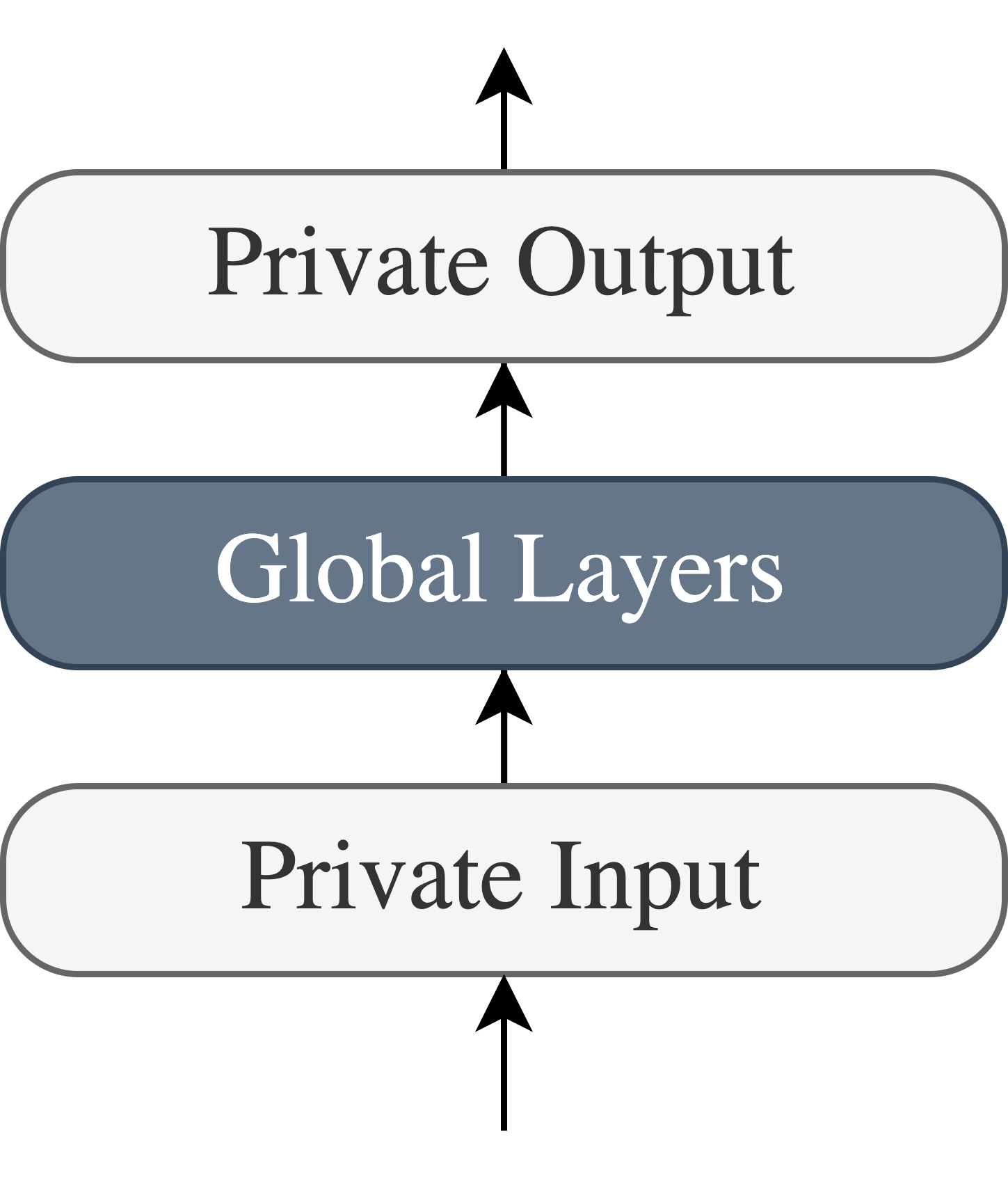
Figure 1: GL high-level architecture. Each client has a local copy of this model. Clients use the full model for inference after training is completed. During training, only the Global Layers are federated. The Private Input and Output layers weights remain local to each client and do not get federated. In general the design of each layer implementation is task dependent. In Figures 2 and 3 we show the model that we empirically found to work well for both experimental settings, with hyperparameters indicated in section E.1.

Earlier we stated the parameters $w_{k}=\{u_{k},\omega,v_{k}\}$ from equations 7 and 8 are architecturally agnostic and should in general be selected like any other neural-network layers, influenced by task choice, complexity, and the extent of statistical heterogeneity. For example, a single linear layer with non-linear activation might be appropriate for each of the private and global layers in certain settings. This point should be explored more in future work. Optimal layer architectures corresponding to particular non-IID FL settings remains as an open question.

In our experimental settings we found superior empirical performance across all settings, including baselines, with the GL model architecture shown in Figure 2. The design is influenced by some recent works investigating methods for tabular data, which we reference. Layer choices and the embedding sizes were selected through hyperparameter optimization with random search cross-validation. We now describe the main components of this model, each shown in more detail in Figure 3.

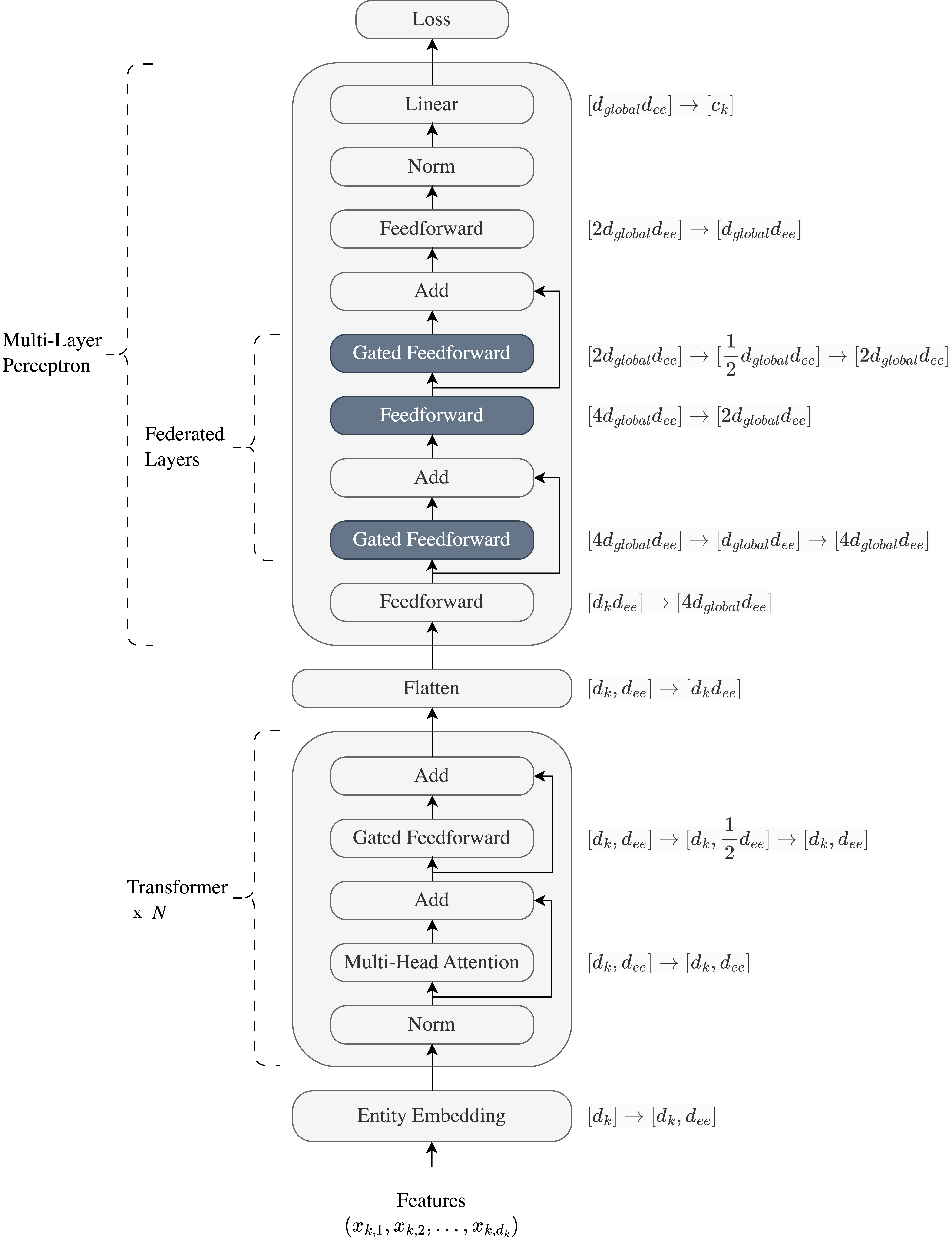
Figure 2: GL model architecture. Federated layers indicated in darker blue shading; other parameters are private. Baseline methods for comparison use an identical architecture, though no parameters are federated for both Local and Centralized settings, and all parameters are federated for the standard FL FedAvg case. Dimension changes as a result of transformations shown on right, corresponding to embedding sizes we used in our experiments. Here, $d_{k}$ and $c_{k}$ are the number of features and classes respectively for client $k$, $d_{global}$ is the global embedding dimension and $d_{ee}$ is the Entity Embedding dimension, also common across all clients. Implementations for Entity Embedding, Feedforward, and Gated Feedforward layers are shown in Figure 3.

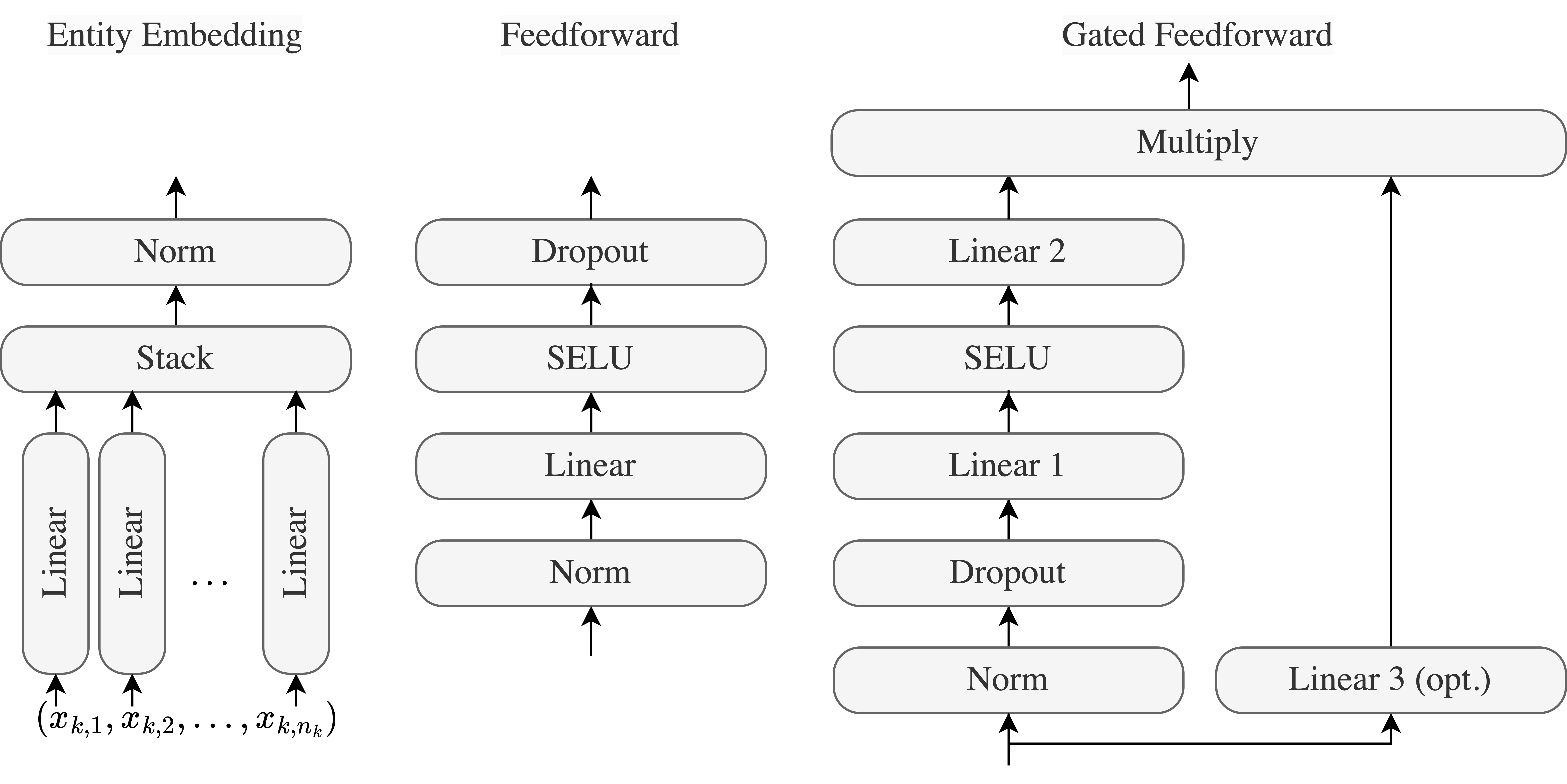
Figure 3: (left) Entity Embedding. (centre) Feedforward. (right) Gated Feedforward.

C.1.1 Entity Embedding

The main idea of Entity Embedding [91] is to map discrete values of a variable to a continuous vector space where relationships between values can be arbitrarily learned. In Equation 9 we show this transformation. The entity embedding dimension, choice of bias for the linear layers and normalization type are hyperparameters. See Figure 3.

Later we describe a preference for ordinal encoding applied to discrete data types. This is justified as following. The use of Entity Embedding and its role in learning relationships of objects within a given category suggests that discrete data types should be kept in their ordinal encoding. One-hot encoding would destroy the class membership category association between discrete object values that Entity Embedding would otherwise use.

C.1.2 Transformer

Our use of Transformer [83] is motivated by Tab-Transformer [44], though [86] is similar, and others referenced in Section 3.3. These works, like ours, use dot-product self-attention to capture complex higher-order feature interactions. Attention mechanisms allow the model to selectively re-weigh feature contributions to the resulting prediction. Exploring different attention mechanisms or their uses, for example SAINT [87] which proposes intrasample attention, is a fruitful area for future work.

A notable work that emphasizes the importance and power of representation learning in the tabular domain is SubTab [97], which recently showed that tabular self-supervised latent representation learning from feature subsets on images in tabular format can outperform CNN-based SOTA models over a 2D image format.

C.1.3 Multi-Layer Perceptron

The original Tab-Transformer specifies a Multi-Layer Perceptron (MLP) implementation consisting of 2 hidden layers and one output layer with sizes $\{4d_{in},2d_{in},d_{c}\}$, where $d_{in}$ is the input size from the previous layer, and $d_{c}$ is the number of classes. This works well with, for example, the UCI Adult dataset in the centralized setting, which was originally reported. However for our non-IID FL experiments we found it necessary to extend this with additional capacity. The embedding sizes we use are shown on the right side of Figure 2, though their selection in general, beyond our experimental settings, should be treated as hyperparameters.

In GL there are 2 repeating blocks of Feedforward and Gated Feedforward with residual, and an additional Feedforward layer before the linear output layer. The implementations for Feedforward and Gated Feedforward are described next. This grants up to 4 layers with consistent dimensionality across clients that we can be federated assuming only the first Feedforward and final output reflect local client dimensionality. Though it would be more precise to say that in this case 8 linear projections in total are global layer candidates that may be federated.

C.1.4 Feedforward

The Feedforward layer is a normalized linear layer with non-linearity and dropout. In other words, a standard non-linear feedforward projection. See Figure 3. In our experiments we found that Batch Normalization, Scaled Exponential Linear Unit (SELU) [92] activation and no dropout, i.e. set to $0.0$ works well, though again in general these should be treated as hyperparameters.

C.1.5 Gated Feedforward

The Gated Feedforward layer consists of 3 linear projections $w_{gff,1}:\mathbb{R}^{d_{in}}\rightarrow\mathbb{R}^{d_{hidden}}$ and $w_{gff,2}:\mathbb{R}^{d_{hidden}}\rightarrow\mathbb{R}^{d_{in}}$ which project to and from a hidden dimension, generally smaller to encourage learning better representations, and $w_{gff,3}:\mathbb{R}^{d_{in}}\rightarrow\mathbb{R}^{d_{in}}$ which applies multiplicative gating to the former. A non-linearity is applied after the first projection only, we used SELU in our experiments, and dropout before. See Figure 3.

C.2 Federated Layers

We propose that the choice of layers to federate should be treated as any other hyperparameter and selected with cross-validation. The only restriction is that the dimensionality must be consistent across client parameters so that they may be aggregated. We found that typical strategies for hyperparameter selection such as random search with cross-validation works well. Exploring optimal selections of which partial-model parameters to federate within a set of inner consistent-dimension candidates is an important open research question.

C.2.1 Personalizing Global Invariants

In Section 3.2, we propose learning a global equipredictive $\omega$ such that: $P(Y_{k}|v_{k}(\omega(u_{k}(X_{k}))))\,\forall k\in K$, where $u_{k}$ and $v_{k}$ are local input and output layers, respectively. To briefly illustrate how a client may compose and personalize the global $\omega$, consider the following re-paramaterization, where $\circ$ denotes composition and assuming invertible layers.

$$v_{k}\circ(\omega\circ u_{k})=\underset{\hat{v_{k}}}{\underbrace{(v_{k}\circ{v}^{\prime}_{k})}}\circ\left(\underset{\hat{\omega}}{\underbrace{(\omega^{\prime\prime}\circ\omega\circ{\omega}^{\prime})}}\circ\underset{\hat{u_{k}}}{\underbrace{(u^{\prime}_{k}\circ u_{k})}}\right)$$ (10)

If ${v}^{\prime}_{k}=\hat{\omega}^{-1}$ then a client $k$ may disregard the global contribution entirely, and similarly for ${u}^{\prime}_{k}=\hat{\omega}^{-1}$. On the other hand if ${v}_{k}={{v}^{\prime}}^{-1}_{k}$ or ${u}_{k}={{u}^{\prime}}^{-1}_{k}$, then it may ignore local contributions. Finally, either ${v}^{\prime}_{k}={\omega^{\prime\prime}}^{-1}$ or ${\omega^{\prime}}^{-1}={u}^{\prime}_{k}$ allows the client to isolate a specific client-invariant transformation of interest $\omega$ while other clients may use the full $\hat{\omega}$. We leave a full theoretical treatment for future work.

Appendix D Datasets

In this section we elaborate on the datasets used in our experiments. Specifically we describe the construction of 2 sets of datasets that form our 2 experiments. The first is based on the classic Covertype benchmark tabular dataset which was naturally multi-source at the time of collection. The second is a collection of 3 multi-source medical datasets independently collected from 3 different hospitals globally. The datasets may be downloaded from the public repositories given in Table 13.

Justifying this, to the best of our knowledge, there are no prior existing tabular FL benchmark datasets comprising of real-world multi-source clients with natural client feature or class exclusivity. Only 1/4 related non-IID FL works mentioned in Section 1 ran experiments on tabular data [16], and they assumed only disjoint but overlapping feature spaces with a shared target space. Further, their clients were generated from single-source centralized datasets with random feature space and sample partitioning. This type of construction constrains the resulting expressed heterogeneity as explained in Section 4.1 and therefore is not a realistic representation of what may occur in real-world settings.

D.1 Covertype

The original Covertype dataset is tabular format and contains 54 features: 40 one-hot encoded columns representing soil types, 4 one-hot encoded columns representing wilderness area, 3 columns represent morning, midday and afternoon shade, and 7 other numerical columns. The task is to predict one of 7 classes representing forest cover types.

Feature	Type
elevation	float32
aspect	float32
slope	float32
hhdist	float32
vhdist	float32
hrdist	float32
hfpdist	float32
soil_type	int
climate_zone	int
geological_zone	int
wilderness_area	int

Table 3: Constructed "Covertype11" dataset features and their data type. Numerical feature names correspond to original dataset feature names.

D.1.1 Pre-processing

As motivated in Section C.1.1, we reversed the pre-existing one-hot encoding into ordinal encoding for two features. The first one was from 40 columns representing soil types which we omit due to length. From these we constructed an additional 2 features. Each column names is 4 digits and the original documentation covtype.info specifies that the first digit represents the climate zone, and the second digit represents the geological zone. The second ordinal feature was wilderness area, reversed from 4 one-hot encoded columns with names: rawah, neota, comanche, poudre. All of these ordinal features are integers types.

To summarize, we converted 40 one-hot columns into 1 ordinal column, from this feature generated 2 more, and finally converted 4 columns to 1 ordinal feature we use as a partition key and drop. We drop the 3 shade columns. The 7 numerical features are all encoded as float32 but otherwise they remain unchanged. In total, before partitioning i.e. with a centralized dataset we are left with the 11 features shown in Table 3.

After cross-validation and client partitioning, ordinal features were ordinal encoded, numerical features were standardized and normalized and targets were label encoded. All encoders were fitted privately and only to the training cross-validation split. The ordinal encoder default missing value was set to $-1$. We used Scikit-Learn’s implementation [98] for all 3 encoders.

D.1.2 Cross-Validation

We re-use the same train/test/validation splits as described in covtype.info with shuffling: first 11,340 records used for training data subset, next 3,780 records used for validation data subset, last 565,892 records used for testing data subset.

D.1.3 Client Partitioning

The Covertype dataset contains samples from 4 distinct regions in the Roosevelt National Forest of northern Colorado. We encourage referencing the original covtype.info documentation from the UCI repository in Table 13 which describes distinct differences between these regions. Therefore we argue such client partitioning is justified by reverting the centralization that was done after initial data collection.

As a result of partitioning, we encountered different but overlapping classes between clients, shown in Table 4. This is not problematic for local-only training or partially-personalized FL methods client-specific outputs layers such as GL. Therefore these are label encoded as normal. However standard FL with full-parameter federation depends on same-sized parameters, so to obtain a comparison result for this case we encode each client with a globally fitted label-encoder. In other words we force alignment between client label spaces for the standard full-model aggregation case with FedAvg.

Dataset	Num.	Local Classes	Local Label-Encoded	Global Label-Encoded
Comanche	6	[1, 2, 3, 5, 6, 7]	[0, 1, 2, 3, 4, 5]	[0, 1, 2, 4, 5, 6]
Neota	3	[1, 2, 7]	[0, 1, 2]	[0, 1, 6]
Poudre	4	[2, 3, 4, 6]	[0, 1, 2, 3]	[1, 2, 3, 5]
Rawah	4	[1, 2, 5, 7]	[0, 1, 2, 3]	[0, 1, 4, 6]
Centralized	7	[1, 2, 3, 4, 5, 6, 7]	[0, 1, 2, 3, 4, 5, 6]	-

Table 4: Class and resulting labels-encoding for Covertype datasets. For local-only and GL, local label-encodings are used. While for standard full-parameter federation, to achieve a consistent output layer dimension necessary for aggregating, we label-encode each client’s local classes with a globally fitted label encoder. The global label encoder has the same classes as the centralized local label-encoded case. This also ensures we do not unintentionally add concept shift and concept drift for the standard FL setting.

D.2 Heart Disease

In this experiment we use 3 distinct datasets that were independently collected at different hospitals globally and at different points in time. The feature spaces are completely disjoint, with no overlap existing between datasets. However, the labels incidentally align. In all datasets, the "0" label corresponds to a patient without heart disease. Nonetheless this experiment remains a challenge that a traditional full-parameter global model $w$, or even a single centralized model without drastic feature engineering, could not address due to dimensional mismatch across input spaces. While we did not explore and compare with possible alternatives such as aligning with missing values, or padding, and this would be valuable future work, these methods are expected to encounter challenges due to the significant, approximately threefold, increase in feature vector dimension they would cause.

Feature	Type
age	int
sex	int
cp	int
trestbps	int
chol	int
fbs	int
restecg	float32
thalach	float32
exang	int
oldpeak	float32
slope	int
ca	int
thal	float32

Table 5: "Cleveland" from UCI Heart Disease, dataset features and their data type.

Feature	Type
sbp	int
tobacco	float32
ldl	float32
adiposity	float32
famhist	int
typea	int
obesity	float32
alcohol	float32
age	int

Table 6: South Africa UCI Heart Disease, dataset features and their data type.

Feature	Type
age	float32
anaemia	int
creatinine_phosphokinase	int
diabetes	int
ejection_fraction	int
high_blood_pressure	int
platelets	float32
serum_creatinine	float32
serum_sodium	int
sex	int
smoking	int
time	int

Table 7: "Faisalabad" from UCI Heart Failure, dataset features and their data type.

D.2.1 UCI Heart Disease, Cleveland

The UCI Heart Disease dataset [94], and in particular the Cleveland dataset, contains 303 patient case studies of coronary heart and artery disease diagnoses collected from the Cleveland Clinic Foundation in the United States between May 1981 and September 1984 [99]. In this task 14 clinical features, shown in Table 5 are used to predict a binary label where $0$ indicates no presence and $1$ indicates presence of heart disease. Out of the 303 patients, 164 are labeled no presence. Note that in the UCI repository there are 2 files: cleveland.data and processed.cleveland.data. The former is described as "corrupted" in the WARNING file in the UCI repository and we thus use the latter.

Besides Cleveland, there are an additional 3 hospital sites: Long Beach VA, Switzerland, and Hungarian, with 200, 123, and 294 instances respectively. We found that inclusion of these smaller datasets as clients would penalize performance for the others and so we focused only on the Cleveland dataset as typically done and described in the original heart-disease.names documentation in the UCI repository. Similarly, while there are 74 features available we focused on the 14 that are typically used, as well as considering only the binary label version.

D.2.2 South Africa Heart Disease

The South Africa Heart Disease dataset is originally from a 1988 retrospective study [100] that contains 462 samples of 9 features from male individuals in high-risk heart disease regions in the Western Cape of South Africa. The goal was to explore prevalence of heart disease in conjunction with high-risk features such as smoking and alcohol consumption in these areas. The features are described in Table 6. Out of the 462 samples, 160 are patients with coronary heart disease, and the remaining 302 are controls. This binary classification task uses $0$ to represent absence, and $1$ to indicate presence of coronary heart disease.

D.2.3 UCI Heart Failure, Faisalabad

The UCI Heart Failure dataset [95] was originally collected [96] during April–December 2015 at the Faisalabad Institute of Cardiology and the Allied Hospital in Faisalabad, Pakistan. It contains 299 patient cases of heart failure, specifically left ventricular systolic dysfunction, with ages ranging from 40-95 and 194 men compared with 105 women. 12 features in total, shown in Table 7 are used to predict a binary target where $1$ indicates a death event, and $0$ means survival. We refer to the original studies for more information.

D.2.4 Pre-processing

No pre-processing was done besides standardization and normalization of numerical features, and ordinal encoding of discrete features with $-1$ for missing values. With one exception. The FedAvg baseline with standard FL cannot support disjoint feature spaces as stated in Section 4.2. Therefore to obtain a result for this case we applied Pandas [101] DataFrame.Align with inputed $0$’s for the padded features belonging to other clients. This results in a consistent feature space which allows full-parameter federation. As we did not create a centralized dataset with such feature space alignment we do not report a centralized baseline for the Heart Disease experiment.

Similar to the Covertype experiment, all encoders were fitted privately and only to the training cross-validation split, and again using Scikit-Learn’s implementation.

D.2.5 Cross-Validation

Cross-validation is achieved first by splitting the original dataset into 70% training and 30% testing, and then another 30% of the split training data used as a validation hold-out set. We again used Scikit-Learn’s traintestsplit implementation with random seed so that each experiment replication generates a new seeded train/test/validation set with shuffling.

D.2.6 Client Partitioning

For the Heart Disease experiment no partitioning was needed as each client is a single-source dataset.

Appendix E Experiments

So far we have described the clients that undergoing FL in each experiment, as well as their model architectures. At the time of developing our experiments, there were no published methods to handle any client input or output space heterogeneity, at all. This motivated the choice of baseline methods we described in Section 4.1.

We developed an experimentation module that would replicate the same model training scenario, with random seed, for each comparison method, given a single launch command. During training, statistics are recorded against the train set after each epoch, as well as a validation set that runs by default each epoch as well. After training, the separate holdout test set is evaluated to produce timeseries metrics for each seeded run, as well as their summary across all runs, and finally a summary over all methods. Runs are fully deterministic and reproducible.

In both experiments we use AdamW optimizer. Covertype is multi-class, so we use Cross-Entropy loss. Heart Disease is binary class, so we use Binary Cross-Entropy. Optimizer, loss and models are implemented with PyTorch.

The number of parameters in each model setting is given in Table 8 for Covertype and Table 9 for Heart Disease.

Each client model is initialized randomly with the same random seed.

	Local		FedAvg		GL
	Num. Param.	Federated	Num. Param.	Federated	Num. Param.	Federated
Comanche	915954	915954	916131	916131	915954	717640
Neota	915954	915954	916131	916131	915423	717640
Poudre	915954	915954	916131	916131	915600	717640
Rawah	915954	915954	916131	916131	915600	717640

Table 8: Number of Model Parameters in Covertype experiment. "Num. Param" corresponds to all model parameters; "Federated" corresponds to the parameters that are aggregated.

	Local		FedAvg		GL
	Num. Param.	Federated	Num. Param.	Federated	Num. Param.	Federated
Cleveland	448339	448339	597415	597415	448339	298688
South Africa	415211	415211	597415	597415	415211	298688
Faisalabad	440057	440057	597415	597415	440057	298688

Table 9: Number of Model Parameters in Heart Disease experiment. "Num. Param" corresponds to all model parameters; "Federated" corresponds to the parameters that are aggregated.

E.1 Hyperparameters

The hyperparameters used in both experiments are provided in Table 10.

Hyperparameter	Value
Entity Embedding Dimension	16
Learning Rate	0.001
Weight Decay	0.0001
Dropout	0.0
Transformer Heads	8
Transformer Blocks	6
$a_{k}$	1.0
Global Layer Update Rate	1.0

Table 10: Hyperparameters used in both experiments.

Hyperparameters particular to Covertype experiment is in Table 11 and for Heart-Disease in Table 12.

Hyperparameter	Value
Epochs	105
Batches	10
Random Seeds	8:28
$d_{global}$	8

Table 11: Hyperparameters used in Covertype experiment.

Hyperparameter	Value
Epochs	10
Batches	15
Random Seeds	0:101
$d_{global}$	$d_{k}=11$
Loss	Binary Cross-Entropy

Table 12: Hyperparameters used in Heart Disease experiment.

E.2 Numerical Results

In Tables 15, 16, and 17 we show numerical results obtained in the experimental settings we have described. Mean, standard deviation and 95% confidence results are provided across 21 and 101 random seeds for Covertype and Heart Disease respectively.

We observe a clear and nearly universal increase in performance and lower variance across AUROC, Accuracy (Balanced Accuracy for Heart Disease), and AUPRC with GL over the baseline methods.

It is interesting to observe that some clients report higher than the centralized baseline in the Covertype experiment. This suggests the personalized global invariants may in fact be more robust than what centralized training alone can learn. This should be explored more in future work, particularly in context of the idea that FL is a natural setting for robust OOD learning [78]. On the other hand, for the Heart Disease experiment there is no baseline method applicable due to disjoint feature spaces. We leave for future work to compare against the case of a composite union of feature spaces as previously mentioned.

E.3 Reproducibility

All experimental code is provided in the following repository: https://github.com/transferFL/gl/.

Documentation to prepare the datasets and run the experiments is provided in the project root README.md.

The four datasets used in the experiments are available on public repositories, provided in Table 13. These are already available in our code repository, however they may also be re-downloaded and placed into folders according to the README.md. Table 14 links to the folders in our code repository containing the exact dataset files we used.

Original Dataset	Source URL
Covertype	https://archive.ics.uci.edu/ml/datasets/covertype
Heart Disease (Cleveland)	https://archive.ics.uci.edu/ml/datasets/Heart+Disease
South Africa Heart Disease	http://statweb.stanford.edu/t̃ibs/ElemStatLearn/data.html
Heart Failure (Faisalabad)	https://archive.ics.uci.edu/ml/datasets/Heart+failure+clinical+records

Table 13: Original dataset source URLs.

Experiment	Source URL
Covertype	https://github.com/transferFL/gl/tree/main/cover/data
Heart Disease	https://github.com/transferFL/gl/tree/main/heart/data

Table 14: URLs to datasets used in our experiments.

The numerical results in Tables 2, 15, 16, and 17 will be replicated exactly when the random seeds specified in Section E.1 are used with a CPU device, Torch 2.1.0 with Python 3.11.2.

Each experiment may be launched with a single command provided in the README.md.

		AUROC (%)
Experiment	Dataset	Local	FedAvg	GL
Covertype (n=21)	Comanche	$88.29\pm 8.36\;(3.58)$	$79.58\pm 7.89\;(3.37)$	$\mathbf{92.09\pm 0.80\;(0.34)}$
	Neota	$79.44\pm 9.46\;(4.05)$	$60.92\pm 2.03\;(0.87)$	$\mathbf{88.85\pm 1.90\;(0.81)}$
	Poudre	$86.74\pm 1.63\;(0.70)$	$63.89\pm 3.33\;(1.42)$	$\mathbf{88.88\pm 1.53\;(0.65)}$
	Rawah	$88.86\pm 1.53\;(0.65)$	$69.82\pm 3.76\;(1.61)$	$\mathbf{91.43\pm 0.65\;(0.28)}$
	Centralized	$88.93\pm 10.71\;(4.58)$	$-$	$-$
Heart Disease (n=101)	Cleveland	$88.57\pm 3.11\;(0.61)$	$\mathbf{89.67\pm 2.61\;(0.51)}$	$89.59\pm 2.89\;(0.56)$
	South Africa	$74.49\pm 3.82\;(0.75)$	$71.13\pm 4.44\;(0.87)$	$\mathbf{76.02\pm 3.70\;(0.72)}$
	Faisalabad	$85.64\pm 4.09\;(0.80)$	$83.68\pm 4.59\;(0.90)$	$\mathbf{86.77\pm 3.80\;(0.74)}$

Table 15: Mean and standard deviation cross-validation result reported across 21, 101 random seeds for Covertype, Heart Disease respectively. 95% confidence interval shown in parenthesis.

		(Balanced) Accuracy1 (%)
Experiment	Dataset	Local	FedAvg	GL
Covertype (n=21)	Comanche	$80.82\pm 6.95\;(2.97)$	$80.46\pm 4.98\;(2.13)$	$\mathbf{83.81\pm 0.45\;(0.19)}$
	Neota	$76.43\pm 6.67\;(2.85)$	$72.26\pm 6.55\;(2.80)$	$\mathbf{81.13\pm 1.90\;(0.81)}$
	Poudre	$72.57\pm 1.20\;(0.51)$	$72.72\pm 1.51\;(0.65)$	$\mathbf{74.21\pm 0.94\;(0.40)}$
	Rawah	$84.25\pm 0.65\;(0.28)$	$83.65\pm 0.68\;(0.29)$	$\mathbf{85.13\pm 0.44\;(0.19)}$
	Centralized	$79.70\pm 15.55\;(6.63)$	$-$	$-$
Heart Disease (n=101)	Cleveland	$80.23\pm 3.98\;(0.78)$	$78.06\pm 4.27\;(0.83)$	$\mathbf{81.18\pm 3.70\;(0.72)}$
	South Africa	$62.43\pm 3.94\;(0.77)$	$56.15\pm 5.20\;(1.01)$	$\mathbf{63.22\pm 4.22\;(0.82)}$
	Faisalabad	$74.57\pm 5.13\;(1.00)$	$67.66\pm 6.54\;(1.28)$	$\mathbf{75.15\pm 4.79\;(0.93)}$

Table 16: Mean and standard deviation cross-validation result reported across 21, 101 random seeds for Covertype, Heart Disease respectively (¹) Heart Disease binary classification reports balanced accuracy. 95% confidence interval shown in parenthesis.

		AUPRC (%)
Experiment	Dataset	Local	FedAvg	GL
Covertype (n=21)	Comanche	$57.82\pm 10.76\;(4.60)$	$45.37\pm 9.20\;(3.93)$	$\mathbf{65.52\pm 2.56\;(1.09)}$
	Neota	$70.23\pm 12.43\;(5.31)$	$27.88\pm 3.53\;(1.51)$	$\mathbf{83.11\pm 3.61\;(1.54)}$
	Poudre	$67.85\pm 3.53\;(1.51)$	$26.67\pm 2.78\;(1.19)$	$\mathbf{71.83\pm 2.94\;(1.26)}$
	Rawah	$64.94\pm 3.65\;(1.56)$	$31.98\pm 5.15\;(2.20)$	$\mathbf{69.90\pm 3.19\;(1.36)}$
	Centralized	$53.09\pm 13.70\;(5.86)$	$-$	$-$
Heart Disease (n=101)	Cleveland	$89.04\pm 3.59\;(0.70)$	$89.57\pm 3.13\;(0.61)$	$\mathbf{90.29\pm 3.08\;(0.60)}$
	South Africa	$59.71\pm 5.66\;(1.10)$	$54.88\pm 6.13\;(1.20)$	$\mathbf{61.86\pm 5.91\;(1.15)}$
	Faisalabad	$74.34\pm 7.38\;(1.44)$	$71.67\pm 7.60\;(1.48)$	$\mathbf{76.41\pm 6.76\;(1.32)}$

Table 17: Mean and standard deviation cross-validation result reported across 21, 101 random seeds for Covertype, Heart Disease respectively. 95% confidence interval shown in parenthesis.

References

- [1] H. Brendan McMahan, Eider Moore, Daniel Ramage, Seth Hampson, and Blaise Agüera y Arcas. Communication-Efficient Learning of Deep Networks from Decentralized Data, February 2017. arXiv:1602.05629 [cs.LG].
- [2] Peter Kairouz, H. Brendan McMahan, Brendan Avent, Aurélien Bellet, Mehdi Bennis, Arjun Nitin Bhagoji, Kallista Bonawitz, Zachary Charles, Graham Cormode, Rachel Cummings, Rafael G. L. D’Oliveira, Hubert Eichner, Salim El Rouayheb, David Evans, Josh Gardner, Zachary Garrett, Adrià Gascón, Badih Ghazi, Phillip B. Gibbons, Marco Gruteser, Zaid Harchaoui, Chaoyang He, Lie He, Zhouyuan Huo, Ben Hutchinson, Justin Hsu, Martin Jaggi, Tara Javidi, Gauri Joshi, Mikhail Khodak, Jakub Konečný, Aleksandra Korolova, Farinaz Koushanfar, Sanmi Koyejo, Tancrède Lepoint, Yang Liu, Prateek Mittal, Mehryar Mohri, Richard Nock, Ayfer Özgür, Rasmus Pagh, Mariana Raykova, Hang Qi, Daniel Ramage, Ramesh Raskar, Dawn Song, Weikang Song, Sebastian U. Stich, Ziteng Sun, Ananda Theertha Suresh, Florian Tramèr, Praneeth Vepakomma, Jianyu Wang, Li Xiong, Zheng Xu, Qiang Yang, Felix X. Yu, Han Yu, and Sen Zhao. Advances and Open Problems in Federated Learning. Foundations and Trends in Machine Learning Vol 4 Issue 1., March 2021.
- [3] Prayitno, Chi-Ren Shyu, Karisma Trinanda Putra, Hsing-Chung Chen, Yuan-Yu Tsai, K. S. M. Tozammel Hossain, Wei Jiang, and Zon-Yin Shae. A Systematic Review of Federated Learning in the Healthcare Area: From the Perspective of Data Properties and Applications. Applied Sciences, 11(23):11191, January 2021.
- [4] Micah J. Sheller, Brandon Edwards, G. Anthony Reina, Jason Martin, Sarthak Pati, Aikaterini Kotrotsou, Mikhail Milchenko, Weilin Xu, Daniel Marcus, Rivka R. Colen, and Spyridon Bakas. Federated learning in medicine: facilitating multi-institutional collaborations without sharing patient data. Scientific Reports, 10(1):12598, July 2020.
- [5] Yiqiang Chen, Jindong Wang, Chaohui Yu, Wen Gao, and Xin Qin. FedHealth: A Federated Transfer Learning Framework for Wearable Healthcare, May 2021. arXiv:1907.09173 [cs.LG].
- [6] Farzin Haddadpour and Mehrdad Mahdavi. On the convergence of local descent methods in federated learning, December 2019. arXiv:1910.14425 [cs.LG].
- [7] Donald B. Rubin. Estimating causal effects of treatments in randomized and nonrandomized studies. Journal of Educational Psychology, 66(5):688–701, October 1974.
- [8] A Szczepura. Access to health care for ethnic minority populations. Postgraduate Medical Journal, 81(953):141–147, March 2005.
- [9] Aoxiao Zhong, Hao He, Zhaolin Ren, Na Li, and Quanzheng Li. FedDAR: Federated Domain-Aware Representation Learning, September 2022. arXiv:2209.04007 [cs.LG].
- [10] Sai Praneeth Karimireddy, Satyen Kale, Mehryar Mohri, Sashank J. Reddi, Sebastian U. Stich, and Ananda Theertha Suresh. SCAFFOLD: Stochastic Controlled Averaging for Federated Learning, April 2021. arXiv:1910.06378 [cs.LG].
- [11] Yue Zhao, Meng Li, Liangzhen Lai, Naveen Suda, Damon Civin, and Vikas Chandra. Federated Learning with Non-IID Data, 2018. arXiv:1806.00582 [cs.LG].
- [12] Hangyu Zhu, Jinjin Xu, Shiqing Liu, and Yaochu Jin. Federated Learning on Non-IID Data: A Survey, June 2021. arXiv:2106.06843 [cs.LG].
- [13] Tian Li, Anit Kumar Sahu, Manzil Zaheer, Maziar Sanjabi, Ameet Talwalkar, and Virginia Smith. Federated Optimization in Heterogeneous Networks, April 2020. arXiv:1812.06127 [cs.LG].
- [14] Aritra Mitra, Rayana Jaafar, George J. Pappas, and Hamed Hassani. Linear Convergence in Federated Learning: Tackling Client Heterogeneity and Sparse Gradients. In Advances in Neural Information Processing Systems, volume 34, pages 14606–14619. Curran Associates, Inc., 2021.
- [15] Yang Liu, Yan Kang, Tianyuan Zou, Yanhong Pu, Yuanqin He, Xiaozhou Ye, Ye Ouyang, Ya-Qin Zhang, and Qiang Yang. Vertical federated learning. arXiv:2211.12814 [cs.LG].
- [16] Chang Liu, Yuwen Yang, Xun Cai, Yue Ding, and Hongtao Lu. Completely heterogeneous federated learning. arXiv:2210.15865 [cs.LG].
- [17] Alain Rakotomamonjy, Maxime Vono, Hamlet Jesse Medina Ruiz, and Liva Ralaivola. Personalised federated learning on heterogeneous feature spaces. arXiv:2301.11447 [cs.LG].
- [18] Disha Makhija, Xing Han, Nhat Ho, and Joydeep Ghosh. Architecture agnostic federated learning for neural networks. In Proceedings of the 39th International Conference on Machine Learning, pages 14860–14870. PMLR, 2022. ISSN: 2640-3498.
- [19] Jiayun Zhang, Xiyuan Zhang, Xinyang Zhang, Dezhi Hong, Rajesh K. Gupta, and Jingbo Shang. Federated learning with client-exclusive classes. arXiv:2301.00489 [cs.LG].
- [20] Vadim Borisov, Tobias Leemann, Kathrin Seßler, Johannes Haug, Martin Pawelczyk, and Gjergji Kasneci. Deep Neural Networks and Tabular Data: A Survey. IEEE Transactions on Neural Networks and Learning Systems, June 2022. arXiv:2110.01889 [cs.LG].
- [21] Mehryar Mohri, Gary Sivek, and Ananda Theertha Suresh. Agnostic Federated Learning, January 2019. arXiv:1902.00146 [cs.LG].
- [22] Yishay Mansour, Mehryar Mohri, Jae Ro, and Ananda Theertha Suresh. Three Approaches for Personalization with Applications to Federated Learning, July 2020. arXiv:2002.10619 [cs.LG].
- [23] Marcos F. Criado, Fernando E. Casado, Roberto Iglesias, Carlos V. Regueiro, and Senén Barro. Non-IID data and Continual Learning processes in Federated Learning: A long road ahead. Information Fusion, 88:263–280, August 2022.
- [24] Yuyang Deng, Mohammad Mahdi Kamani, and Mehrdad Mahdavi. Distributionally Robust Federated Averaging, February 2021. arXiv:2102.12660 [cs.LG].
- [25] Tian Li, Anit Kumar Sahu, Manzil Zaheer, Maziar Sanjabi, Ameet Talwalkar, and Virginia Smith. FedDANE: A Federated Newton-Type Method, January 2020. arXiv:2001.01920 [cs.LG].
- [26] Sashank Reddi, Zachary Charles, Manzil Zaheer, Zachary Garrett, Keith Rush, Jakub Konečný, Sanjiv Kumar, and H. Brendan McMahan. Adaptive Federated Optimization, September 2021. arXiv: 2003.00295 [cs.LG].
- [27] Sai Praneeth Karimireddy, Martin Jaggi, Satyen Kale, Mehryar Mohri, Sashank J. Reddi, Sebastian U. Stich, and Ananda Theertha Suresh. Mime: Mimicking Centralized Stochastic Algorithms in Federated Learning, June 2021. arXiv:2008.03606 [cs.LG].
- [28] Durmus Alp Emre Acar, Yue Zhao, Ramon Matas Navarro, Matthew Mattina, Paul N. Whatmough, and Venkatesh Saligrama. Federated Learning Based on Dynamic Regularization, November 2021. arXiv:2111.04263 [cs.LG].
- [29] Xinwei Zhang, Mingyi Hong, Sairaj Dhople, Wotao Yin, and Yang Liu. FedPD: A Federated Learning Framework with Optimal Rates and Adaptivity to Non-IID Data. IEEE Transactions on Signal Processing, 69:6055–6070, 2021. arXiv:2005.11418 [cs.LG].
- [30] Tao Yu, Eugene Bagdasaryan, and Vitaly Shmatikov. Salvaging Federated Learning by Local Adaptation, March 2022. arXiv:2002.04758 [cs.LG].
- [31] Kangkang Wang, Rajiv Mathews, Chloé Kiddon, Hubert Eichner, Françoise Beaufays, and Daniel Ramage. Federated Evaluation of On-device Personalization, October 2019. arXiv:1910.10252 [cs.LG].
- [32] Hong-You Chen, Cheng-Hao Tu, Ziwei Li, Han-Wei Shen, and Wei-Lun Chao. On the Importance and Applicability of Pre-Training for Federated Learning, October 2022. arXiv:2206.11488 [cs.LG].
- [33] Isabela Albuquerque, Nikhil Naik, Junnan Li, Nitish Keskar, and Richard Socher. Improving out-of-distribution generalization via multi-task self-supervised pretraining, March 2020. arXiv:2003.13525 [cs.CV].
- [34] Ananya Kumar, Aditi Raghunathan, Robbie Jones, Tengyu Ma, and Percy Liang. Fine-Tuning can Distort Pretrained Features and Underperform Out-of-Distribution, February 2022. arXiv:2202.10054 [cs.LG].
- [35] John Nguyen, Jianyu Wang, Kshitiz Malik, Maziar Sanjabi, and Michael Rabbat. Where to begin? on the impact of pre-training and initialization in federated learning. In Workshop on Federated Learning: Recent Advances and New Challenges (in Conjunction with NeurIPS 2022), 2022.
- [36] Yihan Jiang, Jakub Konečný, Keith Rush, and Sreeram Kannan. Improving Federated Learning Personalization via Model Agnostic Meta Learning, September 2019. arXiv:1909.12488 [cs.LG].
- [37] Fei Chen, Mi Luo, Zhenhua Dong, Zhenguo Li, and Xiuqiang He. Federated Meta-Learning with Fast Convergence and Efficient Communication, December 2019. arXiv:1802.07876 [cs.LG].
- [38] Mikhail Khodak, Maria-Florina Balcan, and Ameet Talwalkar. Adaptive Gradient-Based Meta-Learning Methods, December 2019. arXiv:1906.02717 [cs.LG].
- [39] Alireza Fallah, Aryan Mokhtari, and Asuman Ozdaglar. Personalized Federated Learning: A Meta-Learning Approach, October 2020. arXiv:2002.07948 [cs.LG].
- [40] Tianyi Zhang, Shirui Zhang, Ziwei Chen, and Dianbo Liu. PMFL: Partial Meta-Federated Learning for heterogeneous tasks and its applications on real-world medical records, December 2021. arXiv:2112.05321 [cs.LG].
- [41] Canh T. Dinh, Nguyen H. Tran, and Tuan Dung Nguyen. Personalized Federated Learning with Moreau Envelopes, January 2022. arXiv:2006.08848 [cs.LG].
- [42] Virginia Smith, Chao-Kai Chiang, Maziar Sanjabi, and Ameet S Talwalkar. Federated Multi-Task Learning. In Advances in Neural Information Processing Systems, volume 30. Curran Associates, Inc., 2017.
- [43] Tian Li, Shengyuan Hu, Ahmad Beirami, and Virginia Smith. Ditto: Fair and Robust Federated Learning Through Personalization, June 2021. arXiv:2012.04221 [cs.LG].
- [44] Yutao Huang, Lingyang Chu, Zirui Zhou, Lanjun Wang, Jiangchuan Liu, Jian Pei, and Yong Zhang. Personalized Cross-Silo Federated Learning on Non-IID Data, December 2021. arXiv:2007.03797 [cs.LG].
- [45] Matias Mendieta, Taojiannan Yang, Pu Wang, Minwoo Lee, Zhengming Ding, and Chen Chen. Local Learning Matters: Rethinking Data Heterogeneity in Federated Learning. In 2022 IEEE/CVF Conference on Computer Vision and Pattern Recognition (CVPR), pages 8387–8396, New Orleans, LA, USA, June 2022. IEEE.
- [46] Jian Xu, Xinyi Tong, and Shao-Lun Huang. Personalized federated learning with feature alignment and classifier collaboration. In The Eleventh International Conference on Learning Representations, 2023.
- [47] Canh T. Dinh, Tung T. Vu, Nguyen H. Tran, Minh N. Dao, and Hongyu Zhang. A New Look and Convergence Rate of Federated Multi-Task Learning with Laplacian Regularization, October 2022. arXiv:2102.07148 [cs.LG].
- [48] Yongxin Guo, Xiaoying Tang, and Tao Lin. FedDebias: Reducing the Local Learning Bias Improves Federated Learning on Heterogeneous Data, October 2022. arXiv:2205.13462 [cs.LG].
- [49] Sourasekhar Banerjee, Alp Yurtsever, and Monowar H Bhuyan. Personalized multi-tier federated learning. In Workshop on Federated Learning: Recent Advances and New Challenges (in Conjunction with NeurIPS 2022), 2022.
- [50] Filip Hanzely, Slavomír Hanzely, Samuel Horváth, and Peter Richtarik. Lower Bounds and Optimal Algorithms for Personalized Federated Learning. In Advances in Neural Information Processing Systems, volume 33, pages 2304–2315. Curran Associates, Inc., 2020.
- [51] Filip Hanzely and Peter Richtárik. Federated Learning of a Mixture of Global and Local Models, February 2021. arXiv:2002.05516 [cs.LG].
- [52] Daniel Peterson, Pallika Kanani, and Virendra J. Marathe. Private Federated Learning with Domain Adaptation, December 2019. arXiv:1912.06733 [cs.LG].
- [53] Yuyang Deng, Mohammad Mahdi Kamani, and Mehrdad Mahdavi. Adaptive Personalized Federated Learning, November 2020. arXiv:2003.13461 [cs.LG].
- [54] Matthias Reisser, Christos Louizos, Efstratios Gavves, and Max Welling. Federated Mixture of Experts, July 2021. arXiv:2107.06724 [cs.LG].
- [55] Binbin Guo, Yuan Mei, Danyang Xiao, Weigang Wu, Ye Yin, and Hongli Chang. PFL-MoE: Personalized Federated Learning Based on Mixture of Experts, December 2020. arXiv:2012.15589 [cs.LG].
- [56] Michael Zhang, Karan Sapra, Sanja Fidler, Serena Yeung, and Jose M. Alvarez. Personalized Federated Learning with First Order Model Optimization, March 2021. arXiv:2012.08565 [cs.LG].
- [57] Othmane Marfoq, Giovanni Neglia, Aurélien Bellet, Laetitia Kameni, and Richard Vidal. Federated Multi-Task Learning under a Mixture of Distributions, February 2022. arXiv:2108.10252 [cs.LG].
- [58] Jie Zhang, Song Guo, Xiaosong Ma, Haozhao Wang, Wencao Xu, and Feijie Wu. Parameterized knowledge transfer for personalized federated learning. arXiv:2111.02862 [cs.LG].
- [59] Yue Tan, Guodong Long, Lu Liu, Tianyi Zhou, Qinghua Lu, Jing Jiang, and Chengqi Zhang. FedProto: Federated Prototype Learning across Heterogeneous Clients, March 2022. arXiv:2105.00243 [cs.LG].
- [60] Krishna Pillutla, Kshitiz Malik, Abdelrahman Mohamed, Michael Rabbat, Maziar Sanjabi, and Lin Xiao. Federated Learning with Partial Model Personalization, August 2022. arXiv:2204.03809 [cs.LG].
- [61] Tailin Zhou, Jun Zhang, and Danny Tsang. FedFA: Federated Learning with Feature Anchors to Align Feature and Classifier for Heterogeneous Data, December 2022. arXiv:2211.09299v1 [cs.LG].
- [62] Paul Pu Liang, Terrance Liu, Liu Ziyin, Nicholas B. Allen, Randy P. Auerbach, David Brent, Ruslan Salakhutdinov, and Louis-Philippe Morency. Think Locally, Act Globally: Federated Learning with Local and Global Representations, July 2020. Number: arXiv:2001.01523 [cs.LG].
- [63] Manoj Ghuhan Arivazhagan, Vinay Aggarwal, Aaditya Kumar Singh, and Sunav Choudhary. Federated Learning with Personalization Layers, December 2019. arXiv:1912.00818 [cs.LG].
- [64] Liam Collins, Hamed Hassani, Aryan Mokhtari, and Sanjay Shakkottai. Exploiting Shared Representations for Personalized Federated Learning, August 2021. arXiv:2102.07078v2 [cs.LG].
- [65] Hong-You Chen and Wei-Lun Chao. On Bridging Generic and Personalized Federated Learning for Image Classification, July 2022. arXiv:2107.00778 [cs.LG].
- [66] Liangze Jiang and Tao Lin. Test-Time Robust Personalization for Federated Learning, October 2022. arXiv:2205.10920v2 [cs.LG].
- [67] Karan Singhal, Hakim Sidahmed, Zachary Garrett, Shanshan Wu, Keith Rush, and Sushant Prakash. Federated Reconstruction: Partially Local Federated Learning, April 2022. arXiv:2102.03448 [cs.LG].
- [68] Gilles Blanchard, Gyemin Lee, and Clayton Scott. Generalizing from several related classification tasks to a new unlabeled sample. In Advances in Neural Information Processing Systems, volume 24. Curran Associates, Inc., 2011.
- [69] Krikamol Muandet, David Balduzzi, and Bernhard Schölkopf. Domain Generalization via Invariant Feature Representation, January 2013. arXiv:1301.2115 [stat.ML].
- [70] Storkey Amos. When training and test sets are different: Characterizing learning transfer. In Joaquin Quiñonero-Candela, Masashi Sugiyama, Anton Schwaighofer, and Neil D. Lawrence, editors, Dataset Shift in Machine Learning, pages 2–28. The MIT Press, 2008.
- [71] Martin Arjovsky. Out of Distribution Generalization in Machine Learning, March 2021. arXiv:2103.02667 [stat.ML].
- [72] Masanori Koyama and Shoichiro Yamaguchi. When is invariance useful in an out-of-distribution generalization problem?, November 2021. arXiv:2008.01883 [stat.ML].
- [73] Qitian Wu, Hengrui Zhang, Junchi Yan, and David Wipf. Handling distribution shifts on graphs: An invariance perspective. arXiv:2202.02466 [cs.LG].
- [74] V. Vapnik. Principles of Risk Minimization for Learning Theory. In Advances in Neural Information Processing Systems, volume 4. Morgan-Kaufmann, 1991.
- [75] Ishaan Gulrajani and David Lopez-Paz. In search of lost domain generalization, August 2020. arXiv:2007.01434 [cs.LG].
- [76] Kia Khezeli, Arno Blaas, Frank Soboczenski, Nicholas Chia, and John Kalantari. On Invariance Penalties for Risk Minimization, June 2021. arXiv:2106.09777 [cs.LG].
- [77] David Krueger, Ethan Caballero, Joern-Henrik Jacobsen, Amy Zhang, Jonathan Binas, Dinghuai Zhang, Remi Le Priol, and Aaron Courville. Out-of-Distribution Generalization via Risk Extrapolation (REx), February 2021. arXiv:2003.00688 [cs.LG].
- [78] Sreya Francis, Irene Tenison, and Irina Rish. Towards Causal Federated Learning for Enhanced Robustness and Privacy, 2021. arXiv:2104.06557 [cs.LG].
- [79] Xueyang Tang, Song Guo, and Jie Zhang. Exploiting Personalized Invariance for Better Out-of-distribution Generalization in Federated Learning, November 2022. arXiv:2211.11243 [cs.LG].
- [80] Artur Back de Luca, Guojun Zhang, Xi Chen, and Yaoliang Yu. Mitigating Data Heterogeneity in Federated Learning with Data Augmentation, June 2022. arXiv:2206.09979 [cs.LG].
- [81] Jason Yosinski, Jeff Clune, Yoshua Bengio, and Hod Lipson. How transferable are features in deep neural networks? arXiv:1411.1792 [cs.LG].
- [82] Roman Levin, Valeriia Cherepanova, Avi Schwarzschild, Arpit Bansal, C. Bayan Bruss, Tom Goldstein, Andrew Gordon Wilson, and Micah Goldblum. Transfer learning with deep tabular models. arXiv:2206.15306 [cs.LG].
- [83] Ashish Vaswani, Noam Shazeer, Niki Parmar, Jakob Uszkoreit, Llion Jones, Aidan N. Gomez, Lukasz Kaiser, and Illia Polosukhin. Attention Is All You Need, December 2017. arXiv:1706.03762 [cs.CL].
- [84] Yury Gorishniy, Ivan Rubachev, Valentin Khrulkov, and Artem Babenko. Revisiting Deep Learning Models for Tabular Data, November 2021. arXiv:2106.11959 [cs.LG].
- [85] Yuanfei Luo, Hao Zhou, Wei-Wei Tu, Yuqiang Chen, Wenyuan Dai, and Qiang Yang. Network on network for tabular data classification in real-world applications. In Proceedings of the 43rd International ACM SIGIR Conference on Research and Development in Information Retrieval. ACM, July 2020.
- [86] Shenghao Zheng, Xuefeng Xian, Yongjing Hao, Victor S. Sheng, Zhiming Cui, and Pengpeng Zhao. Exploiting Intra and Inter-field Feature Interaction with Self-Attentive Network for CTR Prediction. In Wenjie Zhang, Lei Zou, Zakaria Maamar, and Lu Chen, editors, Web Information Systems Engineering – WISE 2021, volume 13081, pages 34–49. Springer International Publishing, Cham, 2021. Series Title: Lecture Notes in Computer Science.
- [87] Gowthami Somepalli, Micah Goldblum, Avi Schwarzschild, C. Bayan Bruss, and Tom Goldstein. SAINT: Improved Neural Networks for Tabular Data via Row Attention and Contrastive Pre-Training, June 2021. arXiv:2106.01342 [cs.LG].
- [88] Yuexiang Xie, Zhen Wang, Yaliang Li, Bolin Ding, Nezihe Merve Gürel, Ce Zhang, Minlie Huang, Wei Lin, and Jingren Zhou. FIVES: Feature Interaction Via Edge Search for Large-Scale Tabular Data, June 2021. arXiv:2007.14573 [cs.LG].
- [89] Yury Gorishniy, Ivan Rubachev, and Artem Babenko. On Embeddings for Numerical Features in Tabular Deep Learning, March 2022. arXiv:2203.05556 [cs.LG].
- [90] Sergey Ioffe and Christian Szegedy. Batch Normalization: Accelerating Deep Network Training by Reducing Internal Covariate Shift, March 2015. arXiv:1502.03167 [cs.LG].
- [91] Cheng Guo and Felix Berkhahn. Entity Embeddings of Categorical Variables, April 2016. arXiv:1604.06737 [cs.LG].
- [92] Günter Klambauer, Thomas Unterthiner, Andreas Mayr, and Sepp Hochreiter. Self-normalizing neural networks. arXiv:1706.02515 [cs.LG].
- [93] Ilya Loshchilov and Frank Hutter. Decoupled weight decay regularization, January 2019. arXiv:1711.05101 [cs.LG].
- [94] Robert Detrano, Andras Janosi, Walter Steinbrunn, Matthias Pfisterer, Johann-Jakob Schmid, Sarbjit Sandhu, Kern H. Guppy, Stella Lee, and Victor Froelicher. International application of a new probability algorithm for the diagnosis of coronary artery disease. American Journal of Cardiology, 64(5):304–310, 1989. Publisher: Elsevier.
- [95] Davide Chicco and Giuseppe Jurman. Machine learning can predict survival of patients with heart failure from serum creatinine and ejection fraction alone. BMC Medical Informatics and Decision Making, 20(1):16, 2020.
- [96] Tanvir Ahmad, Assia Munir, Sajjad Haider Bhatti, Muhammad Aftab, and Muhammad Ali Raza. Survival analysis of heart failure patients: A case study. PLOS ONE, 12(7):1–8, 2017. Publisher: Public Library of Science.
- [97] Talip Ucar, Ehsan Hajiramezanali, and Lindsay Edwards. SubTab: Subsetting Features of Tabular Data for Self-Supervised Representation Learning, October 2021. arXiv:2110.04361 [cs.LG].
- [98] F. Pedregosa, G. Varoquaux, A. Gramfort, V. Michel, B. Thirion, O. Grisel, M. Blondel, P. Prettenhofer, R. Weiss, V. Dubourg, J. Vanderplas, A. Passos, D. Cournapeau, M. Brucher, M. Perrot, and E. Duchesnay. Scikit-learn: Machine learning in Python. Journal of Machine Learning Research, 12:2825–2830, 2011.
- [99] Hamid Reza Marateb and Sobhan Goudarzi. A noninvasive method for coronary artery diseases diagnosis using a clinically-interpretable fuzzy rule-based system. Journal of Research in Medical Sciences : The Official Journal of Isfahan University of Medical Sciences, 20(3):214–223, 2015.
- [100] J. E. Rossouw, J. P. Du Plessis, A. J. Benadé, P. C. Jordaan, J. P. Kotzé, P. L. Jooste, and J. J. Ferreira. Coronary risk factor screening in three rural communities. the CORIS baseline study. South African Medical Journal, 64(12):430–436, 1983.
- [101] The pandas development team. pandas-dev/pandas: Pandas, February 2020.