Learning without Forgetting for
Vision-Language Models

Abstract

Class-Incremental Learning (CIL) or continual learning is a desired capability in the real world, which requires a learning system to adapt to new tasks without forgetting former ones. While traditional CIL methods focus on visual information to grasp core features, recent advances in Vision-Language Models (VLM) have shown promising capabilities in learning generalizable representations with the aid of textual information. However, when continually trained with new classes, VLMs often suffer from catastrophic forgetting of former knowledge. Applying VLMs to CIL poses two major challenges: 1) how to adapt the model without forgetting; and 2) how to make full use of the multi-modal information. To this end, we propose PROjectiOn Fusion (Proof) that enables VLMs to learn without forgetting. To handle the first challenge, we propose training task-specific projections based on the frozen image/text encoders. When facing new tasks, new projections are expanded and former projections are fixed, alleviating the forgetting of old concepts. For the second challenge, we propose the fusion module to better utilize the cross-modality information. By jointly adjusting visual and textual features, the model can capture semantic information with a stronger representation ability. Extensive experiments on nine benchmark datasets validate Proof achieves state-of-the-art performance.

1 Introduction

In our ever-changing world, training data often comes in a stream format with new classes, requiring a learning system to absorb them continually [19, 18]. To address the challenge of learning emerging new classes, Class-Incremental Learning (CIL) has been proposed [47]. However, in CIL, the absence of former classes triggers catastrophic forgetting [16], where learning new concepts overwrites the knowledge of old ones and results in decline in performance [33]. Numerous efforts have been made [37, 15, 79, 53, 62, 77] to combat catastrophic forgetting in the machine learning field.

With the rapid development of pre-training techniques [20], recent years have witnessed the transition of CIL research from training from scratch [67, 21, 78] to utilizing pre-trained models (PTM) [63, 64, 49]. With the help of PTM, e.g., Vision Transformers [13], incremental models are born with strong transferability to grasp the visual features. Facing the domain gap introduced by the incremental classes, they only need to learn a limited number of additional parameters [26, 11, 34] as the patches to bridge the gap, which significantly simplifies the challenge of incremental learning.

While pre-trained ViT-based CIL methods focus on learning the visual features to recognize new concepts, recent advances in Vision-Language Models (VLM) have demonstrated the potential of textual information in building generalized feature representations. A typical work, i.e., contrastive language-image pre-training [46] (CLIP), maps the visual and textual information in the shared embedding space, enabling robust learning and recognition of concepts from diverse sources. This integration of visual and textual modalities presents a promising avenue for developing continual learning models that can effectively adapt to real-world scenarios.

Extending VLMs to CIL faces two significant challenges. First, sequentially tuning the VLM overwrites the innate generalizability and former concepts, leading to forgetting and poor performance on future tasks. Second, relying solely on textual information for classification neglects the valuable cross-modal features present in the multi-modal inputs. To fully utilize this information, it is necessary to explore methods for cross-modal fusion beyond textual features.

Correspondingly, we aim to turn a VLM into a continual learner that is both retentive and comprehensive. Retentive refers to the model’s ability to maintain its pre-trained capabilities, thereby preserving generalizability and enabling it to perform well on future tasks without forgetting. Comprehensive refers to the model’s capacity to integrate and adjust information from multiple modalities. By leveraging these characteristics, we can mitigate catastrophic forgetting and use cross-modal features to build more robust classifiers as data evolves.

In this paper, we propose PROjectiOn Fusion (Proof) to address catastrophic forgetting in VLM. To make the model retentive, we freeze the pre-trained image/text backbones and append liner projections on top of them. The task-specific information is encoded in the corresponding projection layer by mapping the projected features. When facing new tasks, new projections are extended while old ones are frozen, preserving former knowledge. Besides, we aim to fuse the information from different modalities via cross-model fusion, which allows for the query embedding to be adjusted with context information. Consequently, Proof efficiently incorporates new classes and meanwhile resists forgetting old ones, achieving state-of-the-art performance on nine benchmark datasets. We also investigate the zero-shot performance of VLM with new evaluation protocols and metrics, and find that Proof maintains its zero-shot performance with a simple modification.

2 Related Work

Vision-Language Model (VLM) Tuning: Recent years have witnessed the prosperity of research in VLMs, e.g., CLIP [46], ALIGN [25], CoCa [70], Florence [73], BLIP [31], CLIPPO [54], and Flamingo [1]. These models are pre-trained on vast amounts of images and texts, achieving a unified embedding space across modalities. With great generalizability, they can be applied for downstream tasks in a zero-shot manner. However, a domain gap still exists between the pre-trained and downstream datasets, requiring further tuning for better performance. CoOp and CoCoOp [85, 84] apply prompt learning [32] into VLM tuning with learnable prompt tokens. Subsequent works explore VLM tuning via adapter tuning [17], prompt distribution learning [39], task residual learning [72], similarity learning [76], descriptor learning [42], and optimal transport mapping [10]. However, they only focus on adapting VLM to downstream tasks while overlooking the forgetting of former ones.
Class-Incremental Learning (CIL): aims to learn from evolutive data and absorb new knowledge without forgetting [81]. Replay-based methods [40, 4, 8, 38, 9] save and replay former instances to recover old knowledge when learning new ones. Knowledge distillation-based methods [47, 33, 14] build the mapping between models as regularization. Parameter regularization-based methods [27, 2, 74, 3] weigh the importance of different parameters as regularization. Model rectification-based methods [50, 78, 67, 71] rectify the inductive bias for unbiased predictions. Dynamic networks [69, 58, 82, 59] show strong performance by expanding the network structure as data evolves.
CIL with VLM: Aforementioned CIL methods aim to train an incremental model from scratch, while it would be easier to start with a pre-trained model [30]. The integration of pre-trained Vision Transformer [13] into CIL has attracted the attention of the community, and most methods [63, 64, 49] employ parameter-efficient tuning techniques to learn without forgetting. S-Prompt [61] explores CLIP in domain-incremental learning, but the application of VLM in CIL remains relatively unexplored. WiSE-FT [66] utilizes weight ensemble for robust finetuning, while it cannot be extended to multiple tasks. This paper aims to address this research gap by presenting a comprehensive solution for tuning vision-language models without suffering from forgetting.

3 From Old Classes to New Classes

In this section, we introduce the background information about class-incremental learning and vision language models. We also discuss the naïve solutions for tuning VLM in CIL.

3.1 Class-Incremental Learning

Given a data stream with emerging new classes, class-incremental learning aims to continually incorporate the knowledge and build a unified classifier [81]. We denote the sequence of $B$ training sets without overlapping classes as $\left\{\mathcal{D}^{1},\mathcal{D}^{2},\cdots,\mathcal{D}^{B}\right\}$, where $\mathcal{D}^{b}=\left\{\left({\bf x}_{i},y_{i}\right)\right\}_{i=1}^{n_{b}}$ is the $b$-th training set with $n_{b}$ instances. A training instance ${\bf x}_{i}\in\mathbb{R}^{D}$ belongs to class $y_{i}\in Y_{b}$. $Y_{b}$ is the label space of task $b$, and $Y_{b}\cap Y_{b^{\prime}}=\varnothing$ for $b\neq b^{\prime}$. Following the typical CIL setting [47, 22, 67], a fixed number of exemplars from the former classes are selected as the exemplar set $\mathcal{E}$. During the $b$-th incremental stage, we can only access data from $\mathcal{D}^{b}$ and $\mathcal{E}$ for model training. The target is to build a unified classifier for all seen classes $\mathcal{Y}_{b}=Y_{1}\cup\cdots Y_{b}$ continually. In other words, we hope to find a model $f({\bf x}):X\rightarrow\mathcal{Y}_{b}$ that minimizes the expected risk:

$$f^{*}=\underset{f\in\mathcal{H}}{\operatorname{argmin}}\;\mathbb{E}_{(\mathbf{x},y)\sim\mathcal{D}_{t}^{1}\cup\cdots\mathcal{D}_{t}^{b}}\mathbb{I}\left(y\neq f(\mathbf{x})\right)\,,$$ (1)

where $\mathcal{H}$ denotes the hypothesis space and $\mathbb{I}(\cdot)$ is the indicator function. $\mathcal{D}_{t}^{b}$ denotes the data distribution of task $b$. Following [63, 64, 61], we assume that a pre-trained vision-language model is available as the initialization for $f({\bf x})$, which will be introduced in Section 3.2.

3.2 Vision-Language Model

This paper focuses on contrastive language-image pre-training (CLIP) [46] as the VLM. During pre-training, CLIP jointly learns an image encoder $g_{i}(\cdot):\mathbb{R}^{D}\rightarrow\mathbb{R}^{d}$ and a text encoder $g_{t}(\cdot):\mathbb{R}^{Dt}\rightarrow\mathbb{R}^{d}$ in a contrastive manner, where $D/Dt$ are input dimensions of image/text, and $d$ is the embedding dimension. CLIP projects a batch of image-text pairs into a shared embedding space. It maximizes the cosine similarity of paired inputs and minimizes it for unmatched ones. Benefiting from the massive training data, CLIP can synthesize a zero-shot classifier that generalizes to unseen classes. The output of CLIP is formulated as:

$$p(y_{i}\mid{\bf x})=\frac{\exp\left(\cos\left({\bf z},{\bf w}_{i}\right)/\tau\right)}{\sum_{j=1}^{|\mathcal{Y}_{b}|}\exp\left(\cos\left({\bf z},{\bf w}_{j}\right)/\tau\right)}\,,$$ (2)

where $\cos(\cdot,\cdot)$ denotes cosine similarity, $\tau$ is learnable temperature parameter, ${\bf z}=g_{i}({\bf x})$ is the image embedding. Correspondingly, ${\bf w}_{i}$ is the text embedding of class $y_{i}$ obtained by feeding templated texts, e.g., “a photo of a [CLASS]” into the text encoder. We denote the templated text of class $i$ as $\mathbf{t}_{i}$. Eq. 2 aims to find the most similar text $\mathbf{t}_{i}$ that maximizes the cosine similarity to the query image.

3.3 Overcome Forgetting in Class-Incremental Learning

CIL, as a long-standing problem, has garnered significant attention from the research community. In this section, we introduce two typical solutions for adapting pre-trained models with new classes.

Vision-Based Learning: Traditional CIL methods primarily rely on the image encoder to capture the patterns of new classes. One such method, L2P [64], leverages visual prompt tuning [26] to enable incremental updates of a pre-trained Vision Transformer [13]. By keeping the image encoder frozen, L2P trains a learnable prompt pool $\mathbf{Pool}$ and combines it with patch embeddings to obtain instance-specific embeddings. The optimization target can be formulated as:

$$\mathcal{L}=\ell\left(h\left(\bar{g_{i}}\left({\bf x}_{i},\mathbf{Pool}\right)\right),{y}_{i}\right)+\mathcal{L}_{reg}\,,$$ (3)

where $h(\cdot)$ is the classification head, $\bar{g_{i}}$ is the frozen image encoder, $\mathcal{L}_{reg}$ is the regularization loss for prompt selection. By freezing the encoder, Eq. 3 grasps the new pattern with humble forgetting.

CLIP Tuning: The issue of tuning VLM without forgetting in CIL remains unaddressed, as previous works have solely focused on transferring CLIP to downstream tasks without considering the performance of former tasks. For instance, CoOp [85] converts text inputs into a learnable prompt, i.e., $\mathbf{t}_{i}=$ [V]₁[V]${}_{2}\cdots$[V]_M[CLASS]_i. The posterior probability in Eq. 2 is transformed into:

$$p(y_{i}\mid{\bf x})=\frac{\exp\left(\cos\left({\bf z},g_{t}({\bf t}_{i})\right)/\tau\right)}{\sum_{j=1}^{|\mathcal{Y}_{b}|}\exp\left(\cos\left({\bf z},g_{t}({\bf t}_{j})\right)/\tau\right)}\,.$$ (4)

With the help of the learned prompt, Eq. 4 enables the model to be transferred to the downstream task. However, since the prompt template is shared for all tasks, sequentially tuning CoOp will suffer catastrophic forgetting of former concepts.

Discussions: Current methods focus on different aspects of CIL. Vision-based methods (e.g., Eq. 3) address the issue of forgetting but neglect the valuable semantic information conveyed in texts. Conversely, CLIP’s pre-trained text encoder captures class-wise relationships that can enhance model learning. Meanwhile, transfer learning methods (e.g., Eq. 4) effectively leverage the cross-modal information, while sequentially tuning them suffers the catastrophic forgetting of former concepts. Is it possible to combine the cross-modal information and meanwhile resist catastrophic forgetting?

4 Proof: Projection Fusion for VLM

Observing the limitations of typical vision-based methods in utilizing textual information and forgetting in CLIP tuning, we aim to leverage cross-modality knowledge in CLIP while effectively mitigating forgetting. To this end, we must make the model retentive and comprehensive. Retentive represents the ability to adapt to downstream tasks without forgetting, and we propose projections to map the pre-trained features in the projected feature space. Our unique training strategy ensures the preservation of former knowledge by freezing old projections and expanding new ones for new tasks. The comprehensive aspect involves co-adapting and utilizing cross-modal information to enhance unified predictions. The query instance’s embedding is influenced by both visual and textual information, allowing for instance-specific adaptation and enabling comprehensive predictions.

In the following sections, we introduce the learning paradigm and the co-adaptation process. Lastly, we provide detailed guidelines for training and inference.

4.1 Expandable Feature Projection

CLIP is known for its strong zero-shot performance [46], i.e., Eq. 2 obtains competitive results even without explicit training on the specific tasks. However, given the domain gap between pre-trained and downstream tasks, an adaptation process is still necessary to capture the characteristics of the latter. Specifically, we introduce a linear layer (denoted as “projection”) which is appended after the frozen image and text embeddings to facilitate the matching of pair-wise projected features. Denoting the projection of image/text as $P_{i}(\cdot):\mathbb{R}^{d}\rightarrow\mathbb{R}^{d}$ and $P_{t}(\cdot):\mathbb{R}^{d}\rightarrow\mathbb{R}^{d}$, Eq. 2 is transformed into:

$$p(y_{i}\mid{\bf x})=\underbrace{\frac{\exp\left(\cos\left(P_{i}\left({\bf z}\right),P_{t}\left({\bf w}_{i}\right)\right)/\tau\right)}{\sum_{j=1}^{|\mathcal{Y}_{b}|}\exp\left(\cos\left(P_{i}\left({\bf z}\right),P_{t}\left({\bf w}_{j}\right)\right)/\tau\right)}}_{\text{Projected Matching}}\,.$$ (5)

We denote the classification based on Eq. 5 as $f_{\textbf{PM}}({\bf x})$. By freezing the image and text encoders, it aligns the downstream features in the projected space, allowing the model to encode the relevant downstream information into projection layers. Since the pre-trained model outputs generalizable features, the projection layer learns to recombine features in a data-driven manner. For instance, in a task involving ‘birds,’ the projection would assign a higher weight to features like ‘beaks’ and ‘wings.’ This adaptation enables the projected features to better discern and recognize downstream tasks.

Expandable Projections: However, sequentially training a single projection layer still leads to forgetting of former tasks, resulting in confusion when combining old and new concepts. To this end, we expand task-specific projections for each new task. Specifically, we append a newly initialized projection layer $P_{i}^{b},P_{t}^{b}$ when a new task $\mathcal{D}^{b}$ arrives. This results in a set of projections: $\{P_{i}^{1},P_{i}^{2},\cdots P_{i}^{b},\}$, $\{P_{t}^{1},P_{t}^{2},\cdots P_{t}^{b},\}$, and we adopt the aggregation as the output, i.e.,

$$\textstyle P_{i}({\bf z})=\sum_{m=1}^{b}P_{i}^{m}\left({\bf z}\right),\quad P_{t}({\bf w})=\sum_{n=1}^{b}P_{t}^{n}\left({\bf w}\right)\,.$$ (6)

In Eq. 6, projected features from different stages are mapped and aggregated to capture the different emphases of former and latter tasks. For example, former tasks might emphasize ‘beak’ features for bird recognition, while later tasks may focus on ‘beards’ features to differentiate cats. The aggregation of different projections produces a comprehensive representation of the query instance. By substituting Eq. 6 into Eq. 5, the model aligns the unified features in the joint space.

How to resist forgetting of former projections? To overcome forgetting old concepts, we freeze the projections of former tasks when learning new ones, i.e., $\{\bar{P_{i}^{1}},\bar{P_{i}^{2}},\cdots P_{i}^{b},\}$ (same for $P_{t}$). It allows the newly initialized projection to learn the residual information of new tasks, incorporating new concepts while preserving the knowledge of former ones. During the learning process of task $b$, we optimize the cross-entropy loss to encode the task-specific information into the current projections.

Effect of projections: The illustration of projections are shown in Figure 1 (left). Proof learns projections based on the pre-trained encoders, which fits new patterns and maintains the generalizability of pre-trained model. The parameter number of each projection layer is $d\times d$, which is neglectable for the pre-trained model. Furthermore, the model learns new projections for new tasks, and task-specific projections fit new concepts easily. Since we only optimize the current projections and freeze old ones, the former knowledge is preserved, and forgetting is alleviated.

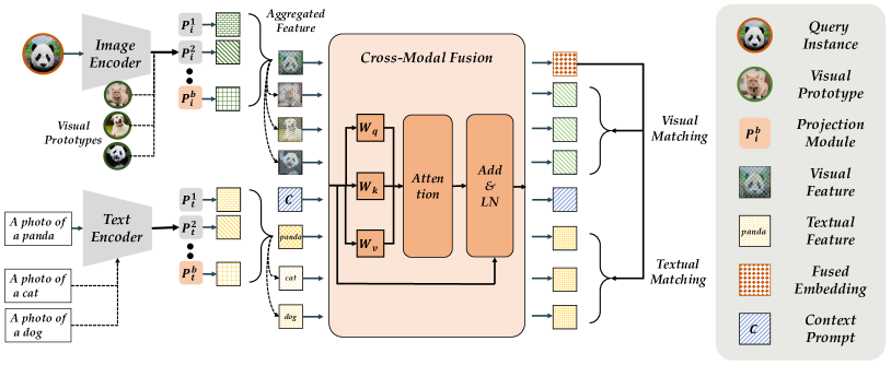
Figure 1: Illustration of Proof. The model learns expandable projections and aggregates them to get the aggregated features. The query instance, prototype features, textual features, and context prompts are fed into the cross-modal fusion. The fusion process utilizes self-attention to co-adapt the input set, which outputs the adapted features. The adapted query embedding is separately matched among the visual prototypes and textual features to get the final prediction. Red parts are trainable while gray ones are frozen.

4.2 Contextualizing Projections with Projection Fusion

In Eq. 5, the projected visual and textual features are directly matched in the joint space. However, it would be beneficial to further refine these features to capture the contextual relationship between images and texts. For instance, when the query instance is a ‘panda,’ it is desirable to adjust the visual and textual features in a coherent manner to highlight discriminative attributes such as black eyes and ears. Similarly, when the query instance is a ‘cat,’ features like beards and tails should be emphasized. This adjustment process involves jointly adapting the query embedding and the context (e.g., textual information) to obtain a contextualized embedding. Correspondingly, we propose a set-to-set function that contextualizes and fuses the query embeddings and contextual information.

Specifically, we denote the adaptation function as $\mathcal{T}(\cdot)$. It receives the query instance and context information as bags, i.e., $[P_{i}({\bf z}),\textbf{Context}]$, and outputs the set of adjusted embeddings while being permutation-invariant: $\mathcal{T}([P_{i}({\bf z}),\textbf{Context}])=[\tilde{P_{i}({\bf z})},\tilde{\textbf{Context}}]$. $\mathcal{T}(\cdot)$ encodes the set information and performs adaptation on each component. In the following, we describe the construction of the context information Context and provide details on the implementation of the set-to-set function.

How to define the context? In Eq. 5, the mapping is established between the query instance and the textual information (i.e., classifiers). The classifiers represent the typical textual description of the corresponding class, i.e., the common feature. Hence, a naïve idea is to utilize textual features as the context, i.e., $\textbf{Context}=\mathbf{W}$, $\mathbf{W}=[P_{t}({\bf w}_{1}),P_{t}({\bf w}_{2}),\cdots,P_{t}({\bf w}_{|\mathcal{Y}_{b}|})]\in\mathbb{R}^{|\mathcal{Y}_{b}|\times d}$ is the concatenation of all textual classifiers. However, recent works find an inherent domain gap [35] between the visual and textual embeddings in VLM. The gap leads to visual and textual embeddings residing in two separate clusters in the embedding space, which hinders effective pair-wise mapping. Correspondingly, we leverage visual prototype features [51] as a useful tool for capturing the common characteristics of each class. Define the visual prototype of class $k$ as: ${\bf p}_{k}=\frac{1}{N}{\sum_{j=1}^{|\mathcal{{D}}^{b}|}\mathbb{I}(y_{j}=k)g_{i}({\bf x}_{j})}$, where $N={\sum_{j=1}^{|\mathcal{{D}}^{b}|}\mathbb{I}(y_{j}=k)}$. They are calculated via forward pass at the beginning of each incremental stage and stay fixed in subsequent tasks. Visual prototypes are representative features of the corresponding class, which can serve as the visual context to adjust the embeddings. Hence, we augment the context with projected visual information, i.e., $\textbf{Context}=[\mathbf{P},\mathbf{W}]$, where $\mathbf{P}=[P_{i}({\bf p}_{1}),P_{i}({\bf p}_{2}),\cdots,P_{i}({\bf p}_{|\mathcal{Y}_{b}|})]\in\mathbb{R}^{|\mathcal{Y}_{b}|\times d}$ is the concatenation of all visual prototypes. Combining prototypes from multiple modalities help the model adapt and fuse information in a cross-modal manner, which goes beyond simple visual-textual matching.

Implementing $\mathcal{T}$ with Self-Attention: In our implementation, we use the self-attention (SA) mechanism [55, 36] as the cross-modal fusion function $\mathcal{T}$. Being permutation invariant, SA is good at outputting adapted embeddings even with long dependencies, which naturally suits the characteristics of the adaptation function. Specifically, SA keeps the triplets (query $\mathcal{Q}$, key, $\mathcal{K}$, and value $\mathcal{V}$). The inputs are projected into the same space, i.e., $K=W_{K}^{\top}\left[\,\mathbf{k}_{k};\,\forall\mathbf{k}_{k}\in\mathcal{K}\,\right]\in\mathbb{R}^{d\times|\mathcal{K}|}$. Similar projections are made for $\mathcal{Q}$ and $\mathcal{V}$. The query ${\bf x}_{q}\in\mathcal{Q}$ is matched against a list of keys $K$ where each key has a value $V$. The output is the sum of all the values weighted by the proximity of the key to the query point:

$$\textstyle\tilde{P}_{i}({\bf z})={P}_{i}({\bf z})+\sum_{k}\alpha_{qk}V_{:,k}\,,$$ (7)

where $\alpha_{qk}\propto\exp\left(\frac{{P}_{i}({\bf z})^{\top}W_{Q}\cdot K}{\sqrt{d}}\right)$, $V_{:,k}$ is the $k$-th column of $V$. The adaptation process is the same for other components in Context. Specifically, we have $\mathcal{Q}=\mathcal{K}=\mathcal{V}=[P_{i}({\bf z}),\textbf{Context}]$.

Effect of Cross-Modal Fusion: The illustration of the projection fusion is shown in Figure 1 (right). We utilize the visual and textual information of seen classes as context information to help adjust the instance-specific embeddings. The fusion model is trained incrementally to adjust embeddings to reflect the context information as data evolves. With the contextualized embeddings, we can conduct the visual mapping and textual matching:

$$p(y_{i}\mid{\bf x})=\underbrace{\frac{\exp\left(\cos\left(\tilde{P}_{i}({\bf z}),\tilde{P}_{i}({\bf p}_{i})\right)/\tau\right)}{\sum_{j=1}^{|\mathcal{Y}_{b}|}\exp\left(\cos\left(\tilde{P}_{i}({\bf z}),\tilde{P}_{i}({\bf p}_{j})\right)/\tau\right)}}_{\text{Visual Matching}}+\underbrace{\frac{\exp\left(\cos\left(\tilde{P}_{i}({\bf z}),\tilde{P}_{t}({\bf w}_{i})\right)/\tau\right)}{\sum_{j=1}^{|\mathcal{Y}_{b}|}\exp\left(\cos\left(\tilde{P}_{i}({\bf z}),\tilde{P}_{t}({\bf w}_{j})\right)/\tau\right)}}_{\text{Textual Matching}}\,.$$ (8)

In Eq. 8, the model assigns logits to the query instance by the similarity to the adapted visual and textual prototypes. The incorporation of cross-modal matching enhances the prediction performance.

Learning Context Prompts: In addition to visual prototypes and textual classifiers, we also introduce a set of learnable context prompts $\{\mathbf{c}^{1},\cdots,\mathbf{c}^{b}\},\mathbf{c}^{i}\in\mathbb{R}^{c\times d}$ to be optimized as data evolves. $c$ denotes the length of each prompt. Similar to projection layers, we make the context prompts expandable to catch the new characteristics of new tasks. We initialize a new context prompt while learning a new task and freeze others $\{\bar{\mathbf{c}}^{1},\bar{\mathbf{c}}^{2},\cdots,{\mathbf{c}^{b}}\}$. The context prompts serve as adaptable context information, enhancing the co-adaption. Hence, the context information is formulated as $\textbf{Context}=[\mathbf{P},\mathbf{W},\mathbf{C}]$, where $\mathbf{C}$ is the aggregation of all context prompts. Note that $\mathbf{C}$ only encodes the task-specific information into the self-attention process, which does not serve as the matching target in Eq. 8.

4.3 Summary of Proof

In Proof, we first enable learning new concepts via projected mapping. Then, to accommodate new concepts without interference from previous ones, we initialize new projections for each new task and freeze the former ones. Besides, we utilize self-attention to adjust the embeddings of the query instance and the context information to promote cross-modal fusion. Figure 1 illustrates three predictions, i.e., projected matching (Eq. 5), visual/textual matching (Eq. 8). We denote these models as $f_{\text{PM}}({\bf x}),f_{\text{VM}}({\bf x}),f_{\text{TM}}({\bf x})$, respectively. During training, we optimize the cross-entropy loss:

$$\textstyle\min_{\{P_{i}^{b},P_{t}^{b},\mathcal{T},\mathbf{c}^{b}\}}\ell(f_{\text{PM}}({\bf x}),y)+\ell(f_{\text{VM}}({\bf x}),y)+\ell(f_{\text{TM}}({\bf x}),y)\,.$$ (9)

In Eq. 9, all pre-trained weights are frozen, and we only optimize these additional parameters. For inference, we aggregate the three logits, i.e., $f({\bf x})=f_{\text{PM}}({\bf x})+f_{\text{VM}}({\bf x})+f_{\text{TM}}({\bf x})$. We give the pseudo-code of Proof in the supplementary.

5 Experiment

In this section, we compare Proof in comparison to state-of-the-art methods on benchmark datasets to investigate the capability of overcoming forgetting. We also conduct ablations to analyze the effect of each component in the model. Furthermore, we address a fundamental issue in VLM training known as zero-shot degradation. Finally, we extend Proof to other VLMs to verify the universality of proposed method. Further details and experimental results can be found in the supplementary.

5.1 Experimental Setup

Dataset: Following the benchmark CIL settings [47, 64, 63, 71, 83], we evaluate the performance on CIFAR100 [29], CUB200 [57], ObjectNet [6], and ImageNet-R [12]. We also follow the setting in VLM tuning [85], and formulate FGVCAircraft [41], StanfordCars [28], Food101 [7], SUN397 [68] and UCF101 [52] into CIL setting. Specifically, we sample (a subset of) 100 classes from CIFAR100, Aircraft, Cars, Food, UCF, 200 classes from CUB200, ObjectNet, ImageNet-R, and 300 classes from SUN to ease the data split. Following [47], the class order of training classes is shuffled with random seed 1993. The dataset splits are denoted as Base-$x$, Inc-$y$, where $x$ represents the number of classes in the first stage, and $y$ represents the number of new classes in each subsequent task. $x=0$ means each task contains $y$ classes. More details are reported in the supplementary.

Comparison methods: We first compare to SOTA CIL methods iCaRL [47], MEMO [82], SimpleCIL [83] L2P [64], DualPrompt [63]. Denote the baseline of sequential finetuning as Finetune; we combine it with different tuning techniques, e.g., LiT [75] and CoOp [85]. We also report the zero-shot performance of CLIP as ZS-CLIP by matching the query instance to the template (Eq. 2).

Implementation details: We deploy all methods with PyTorch [44] and PyCIL [80] on Tesla V100. We use the same network backbone ViT-B/16 for all compared methods for fair comparison. We experiment with two commonly used pre-trained CLIP weights, i.e., OpenAI [46] and OpenCLIP LAION-400M [24]. The model is trained with a batch size of 64 for 5 epochs, and we use SGD with momentum for optimization. The learning rate starts from $0.001$ and decays with cosine annealing. Following [47], we use the herding [65] algorithm to select 20 exemplars per class for rehearsal. The context prompt length is set to 3, and the head of self-attention is set to 1. The template for classification is the same as [43]. The source code will be made publicly available upon acceptance.

Performance Measure: Denote the Top-1 accuracy after the $b$-th stage as $\mathcal{A}_{b}$, we follow [47] to use $\mathcal{A}_{B}$ (last stage performance) and $\bar{\mathcal{A}}=\frac{1}{B}\sum_{b=1}^{B}\mathcal{A}_{b}$ (average performance) for evaluation.

5.2 Benchmark Comparison

We report the results on nine benchmark datasets using ViT-B/16 (OpenCLIP LAION-400M) in Table LABEL:tab:benchmark and Figure LABEL:figure:benchmark. These splits include the scenarios with large and small base classes. Notably, Proof consistently achieves the best performance among all the methods compared. Sequential finetuning of the model with contrastive loss leads to significant forgetting, irrespective of the tuning techniques employed (e.g., LiT and CoOp). Since SimpleCIL and ZS-CLIP do not finetune the model parameters, they achieve competitive results by transferring the knowledge from the pre-training stage into the downstream tasks. However, most methods achieve better performance than ZS-CLIP, indicating the importance of incremental learning on downstream tasks.

Specifically, we can draw three key conclusions from these results. 1) The first stage performance of Proof surpasses that of the typical prompt learning method, CoOp, thus validating the effectiveness of learning projections for downstream tasks. 2) The performance curve of Proof consistently ranks at the top across all methods, demonstrating its capability to resist forgetting. 3) Compared to vision-only methods (i.e., L2P and DualPrompt), Proof exhibits substantial improvement, indicating textual and visual information can be co-adapted to facilitate incremental learning.

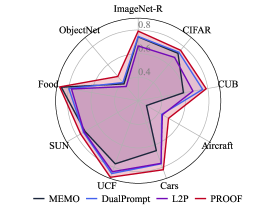
(a) OpenAI weight

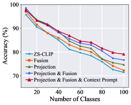
(b) Compositional components

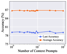
(c) Context prompt length

Figure 2: Ablation study. Left: experiments on 9 benchmarks with OpenAI weights. Middle: ablation study on compositional components in Proof. Every part improves the performance of CIL. Right: $\mathcal{A}_{B}$ and $\bar{\mathcal{A}}$ with change of context prompts. The performance is robust to the change of context prompt length.

5.3 Ablation Study

Different backbone weights: The comparison in Section 5.2 is based on LAION-400M pre-trained CLIP. As another popular pre-trained weight, we also explore the performance of the weights provided by OpenAI. We report the last accuracy $\mathcal{A}_{B}$ of four competitive methods on nine benchmarks in Figure 2(a). We report the full results of the incremental performance in the supplementary. As depicted in the figure, Proof still performs the best on all datasets among all compared methods.

Compositional components: We experiment on CIFAR100 B0 Inc10 to investigate the importance of each part in Proof. Specifically, we compare the performance of Proof and its sub-modules, i.e., projections and cross-modal fusion. The results, shown in Figure 2(b), indicate that training expandable projections or the fusion module individually can both enhance the performance of vanilla CLIP. This suggests that the expandable task representation and cross-modal information can help the learning process. Furthermore, when combining them together, we find ‘Projection & Fusion’ further shows better performance than any of them, verifying that they can work together by fusing the expandable representations. Lastly, when incorporating the context prompts, the model shows the best performance among all variations, verifying the effectiveness of expandable task-specific prompts in incremental learning. Ablations verify the importance of each component in Proof.

Number of context prompts: Figure 2(b) verifies the strong performance of context prompts, and we explore the appropriate length $c$ of the context prompt on CIFAR100 B0 Inc10. By varying the number of $c$ among $\{1,2,3,4,5,6,7,8,9,10,30,50,100\}$, we report the average performance and last performance of Proof in Figure 2(c). As shown in the figure, the performance of Proof is robust with the change of the prompt length, and we set $c=3$ as the default length.

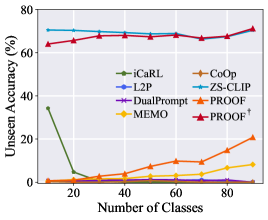
(a) Unseen class accuracy

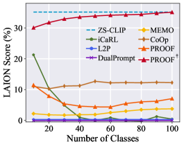
(b) LAION score

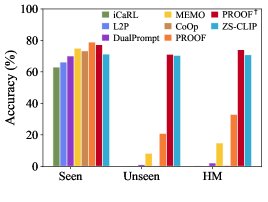
(c) $\mathcal{A}_{\text{S}}\,,\mathcal{A}_{\text{U}}\,,\mathcal{A}_{\text{HM}}$

Figure 3: Experiment on zero-shot performance. Left: accuracy on unseen classes during incremental learning. Middle: LAION score during incremental learning. Right: accuracy of seen, unseen, and harmonic mean (HM) at the last incremental stage. Proof^† strikes a balance between adaptivity and the ZS performance.

5.4 Exploring Zero-Shot Performance

CLIP is known to have the zero-shot (ZS) ability, i.e., even if the model has not been trained for recognizing the image, it can still predict the possibility of an image ${\bf x}$ belonging to the class $y$ by matching the cosine similarity via Eq. 2. The strong generalizability of CLIP makes it a popular model in computer vision. However, in CIL, the model is continuously updated with the downstream task, which weakens the generalizability and harms the ZS performance [66] on subsequent tasks. In this section, we explore the ZS performance degradation of CLIP and propose a variation of Proof to maintain the ZS performance.

Evaluation protocol for ZS performance: Current CIL methods focus on evaluating ‘seen’ classes, i.e., evaluating $\mathcal{Y}_{b}=Y_{1}\cup\cdots Y_{b}$ after learning task $b$. However, since CLIP exhibits ZS performance, we can also assess the performance on ‘unseen’ classes $\mathcal{Y}_{u}=Y_{b+1}\cup\cdots Y_{B}$ to investigate the ZS performance. Correspondingly, we can obtain the performance metrics $\mathcal{A}_{\text{S}}$ (seen classes), $\mathcal{A}_{\text{U}}$ (unseen classes), and $\mathcal{A}_{\text{HM}}$ (harmonic mean of $\mathcal{A}_{S}$ and $\mathcal{A}_{U}$) after each task. Additionally, based on the LAION400M [48] pre-trained CLIP, we also utilize a subset of 10,000 image-text pairs from LAION400M, and calculate the matching score of them, i.e., cosine similarity of image-text embeddings. We denote the average matching score as LAION score, which indicates the matching degree of the adapted model on the upstream tasks. Given the relationship between generalizability and the upstream task, the LAION score serves as an effective measure of ZS performance.

Results: We compare the aforementioned measures on CIFAR100 B0 Inc10. Apart from compared methods in Section 5.2, we also report a variation of Proof, namely Proof^†. The only difference lies in the design of the projection, where Proof^† uses a residual format $P_{i}({\bf z})=\sum_{m=1}^{b}\left(P_{i}^{m}\left({\bf z}\right)+{\bf z}\right)$ as the output (same for $P_{t}$). To investigate the ZS performance as model updates, we show the accuracy on unseen classes $\mathcal{A}_{\text{U}}$ along incremental stages in Figure 3(a), where ZS-CLIP shows the best performance. Due to the incorporation of pre-trained information into the projected features, Proof^† maintains competitive ZS performance. Conversely, other methods experience a decline in ZS performance as their focus shifts to downstream tasks. We observe a similar trend in Figure 3(b), where Proof^† achieves a LAION score similar to that of ZS-CLIP. Lastly, we report $\mathcal{A}_{\text{S}},\mathcal{A}_{\text{U}},\mathcal{A}_{\text{HM}}$ in the last incremental stage in Figure 3(c). We can infer a trade-off between the adaptivity on downstream tasks and the generalizability of ZS performance. Compared to Proof, Proof^† sacrifices the adaptivity to maintain ZS performance, strikings a balance between seen and unseen classes. Therefore, when ZS performance is essential, using Proof^† is the preferred choice.

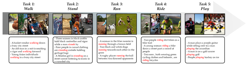
Figure 4: The training protocol of five incremental stages in Flickr30K. We split training instances into five tasks, i.e., walk, stand, run, ride, and play. The training/testing sets do not include images that do not fall into these tasks. We use the pre-trained BEiT-3 as the initialization and sequentially learn cross-modal retrieval tasks. At the end of each task, the model is evaluated on all previously learned concepts.

Table 1: Average and last performance of different methods. The best is in bold. The first row stands for the text retrieval task, and the second is the image retrieval task.

Method	Image $\rightarrow$ Text
	$R_{B}@1$	$\bar{R}@1$	$R_{B}@5$	$\bar{R}@5$	$R_{B}@10$	$\bar{R}@10$
Finetune	48.79	62.89	76.38	85.04	85.68	91.84
DER [69]	78.37	84.48	96.34	98.23	99.06	99.59
MEMO [82]	83.18	87.79	96.57	98.27	99.16	99.66
Proof	85.68	89.43	97.07	98.68	99.79	99.86

Method	Text $\rightarrow$ Image
	$R_{B}@1$	$\bar{R}@1$	$R_{B}@5$	$\bar{R}@5$	$R_{B}@10$	$\bar{R}@10$
Finetune	37.35	51.33	67.38	77.77	77.95	85.55
DER [69]	66.71	74.18	89.63	93.00	94.84	96.69
MEMO [82]	69.53	76.35	91.89	94.44	96.09	97.32
Proof	72.10	78.01	93.10	95.27	96.92	97.90

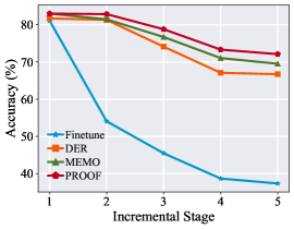
(a) IR@1

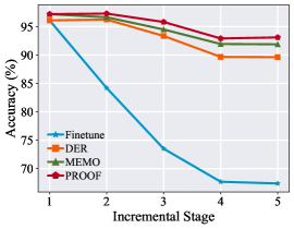
(b) IR@5

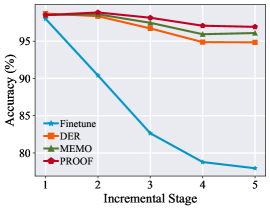
(c) IR@10

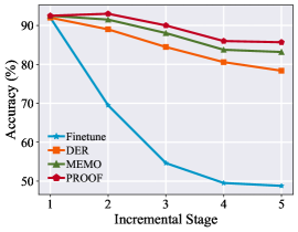
(d) TR@1

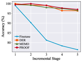
(e) TR@5

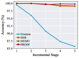
(f) TR@10

Figure 5: Incremental performance of each method. IR means the recall of image retrieval, and TR denotes the recall of text retrieval. Proof consistently outperforms other compared methods with a substantial margin on the incremental cross-modal retrieval task.

5.5 Extension to Other Vision Language Models

In the main paper, we use CLIP as an exemplar VLM due to its popularity and representativeness. However, the field of vision-language models is rapidly advancing, and various models are available. Therefore, in this section, we extend our Proof framework to another widely used vision-language model, namely BEiT-3 [60], focusing on the cross-modal retrieval task. BEiT-3 is a popular VLM that demonstrates promising performance across multiple vision-language tasks. When fine-tuning BEiT-3 for cross-modal retrieval, it functions as a dual encoder, similar to CLIP, featuring a dual-branch structure. As the retrieval task differs from classification, we adopt a degradation of Proof by solely employing the projection expansion strategy without implementing cross-modal fusion. We refer the readers to the BEiT-3 paper [60] for more details about the backbone model.

For evaluation, we employ the Flickr30K dataset [45] to assess the performance of incremental cross-modal retrieval. Flickr30K comprises 31,783 images collected from the Flickr image-sharing platform, encompassing diverse themes such as daily life, travel, people, food, and scenes. Each image in the dataset is accompanied by five manually annotated textual descriptions, which provide descriptive information capturing the main content and context of the images. To formulate an incremental data stream, we utilize keyword matching to identify images containing different actions (e.g., walk, stand, run, ride, play). Then, we split the training instances into five subsets based on these specific actions. Figure 4 illustrates the formulation of the stream, while images not associated with these actions are excluded from training. To create a balanced testing set, we maintain a 5:1 training-to-testing ratio for splitting the training and testing pairs. Following the instructions provided by BEiT, we use ‘beit3_base_itc_patch16_224’ as the VLM’s initialization.

For evaluation, we employ standard cross-modal retrieval measures, namely $R@1$, $R@5$, and $R@10$. The retrieval is conducted in two directions: image $\rightarrow$ text and text $\rightarrow$ image. Similarly to the CIL evaluation, we also report the last recall $R_{B}@1$ and the average recall $\bar{R}@1$ across incremental stages. To provide a comparative analysis, we compare Proof against typical fine-tuning as the baseline and modify MEMO [82] and DER [69] for comparison. These methods represent state-of-the-art CIL approaches that can be adapted with minor modifications to the current task. However, methods such as L2P and DualPrompt are unsuitable for cross-modal retrieval tasks as they do not focus on cross-modal matching.

The experimental results are presented in Table 1, and the incremental performance of each measure is depicted in Figure 5. As evident from these figures, fine-tuning the model with new concepts leads to catastrophic forgetting in cross-modal retrieval tasks. However, equipping the model with incremental learning abilities alleviates forgetting. Among all the compared methods, Proof consistently achieves the best performance across different retrieval tasks and metrics, thereby verifying its effectiveness in mitigating forgetting in VLMs. Experiments conducted on different VLMs and tasks establish Proof as a unified and general framework. Future work involves extending Proof to other VLMs and applications, such as image captioning [56] and VQA [5].

6 Conclusion

Real-world learning systems necessitate the ability to continually acquire new knowledge. In this paper, we aim to equip the popular VLM with the CIL ability. Specifically, we learn the expandable projections so that visual and textual information can be aligned incrementally. This expansion technique allows for the integration of new concepts without compromising previous ones. Additionally, we enforce cross-modality fusion with self-attention mechanism, where visual and textual information are jointly adapted to produce instance-specific embeddings. Extensive experiments validate the effectiveness of our proposed Proof. Furthermore, we demonstrate that a simple variation of Proof preserves the model’s zero-shot capability during updating.
Limitations: Possible limitations include the usage of exemplars, where storage constraints and privacy issues may happen. Future works include extending the model to exemplar-free scenarios.

Supplementary Material

In the main paper, we present a method to prevent forgetting in vision-language models through projection expansion and fusion. The supplementary material provides additional details on the experimental results mentioned in the main paper, along with extra empirical evaluations and discussions. The organization of the supplementary material is as follows:

• Section A presents the pseudo code of Proof, explaining the training and testing pipeline.

• Section B reports comprehensive experimental results from the main paper, including the full results of nine benchmark datasets with two data splits, as well as the results obtained using OpenAI weights. Furthermore, this section includes additional ablations such as variations of projection types, results from multiple runs, and an analysis of the number of parameters.

• Sections C and D provide detailed information on the experiments, including dataset and exemplar selection details, an introduction to the compared methods, and a discussion of the broader impacts.

A Pseudo Code

In this section, we provide a detailed explanation of Proof by presenting the pseudo-code in Alg 1. In each incremental stage, we are provided with the training dataset $\mathcal{D}^{b}$ and the exemplar set $\mathcal{E}$, with the objective of updating the current model $f(\cdot)$. Prior to training, we initially extract visual prototypes for the new classes (Line 1). These prototypes are calculated using the frozen visual embedding $g_{i}(\cdot)$, ensuring their stability throughout model updates. Subsequently, we freeze the former projections and context prompts, while initializing new projections and context prompts specifically for the new incremental task (Line 2 to Line 4). These steps represent the model expansion process, which is followed by the subsequent learning process.

During the learning process, we concatenate the training instances from the current dataset and the exemplar set, initiating a for-loop. For each instance-label pair, we calculate the projected visual and textual embeddings (Line 6 to Line 9). Subsequently, we compute the projected matching loss (Line 10) to encode task-specific information into the current projection layers. Based on the projected features, we derive context information and perform cross-modal fusion (Line 11 to Line 13). Consequently, we obtain three logits for model updating and utilize the cross-entropy loss to update these modules (Line 14). The updated model is then returned as the output of the training process.

Discussions: Besides the simple addition operation, there exist alternative methods for aggregating information from multiple projections. However, due to the requirement of fixed input dimensionality for cross-modal fusion, we refrain from using concatenation as the aggregation function. Furthermore, it is worth noting that MEMO [82] can be viewed as a specific case where concatenation is employed for aggregation. Nonetheless, its inferior performance (as shown in Table 2) suggests that summation is a more favorable choice.

Algorithm 1 Training Proof for CIL

Input: Training dataset: $\mathcal{D}^{b}$; Exemplar set: $\mathcal{E}$; Current model: $f(\cdot)$;
Output: Updated model;

1:Extract prototypes $\mathbf{p}$ for each new class in $\mathcal{D}^{b}$;

2:Freeze current projections and context prompts;

3:Initialize new projections for the visual and textual branches, $P_{i}^{b},P_{t}^{b}$; $\triangleright$ Expand projections

4:Initialize new context prompt $\mathbf{c}^{b}$;

5:for $({\bf x},y)\in\mathcal{D}^{b}\cup\mathcal{E}$ do $\triangleright$ Incremental learning

6:     Calculate the visual embedding ${\bf z}=g_{i}({\bf x})$;

7:     Calculate the projected visual feature $P_{i}({\bf z})$;

8:     Calculate the textual embedding ${\bf w}$ of all seen classes;

9:     Calculate the projected textual embeddings of all seen classes $P_{t}({\bf w})$;

10:     Calculate the logits for projected matching $f_{\textbf{PM}}({\bf x})$ via Eq. 5;$\triangleright$ Projected matching

11:     Calculate the projected visual features for all visual prototypes ${\bf p}$;

12:     Conduct cross-modal fusion via Eq. 7; $\triangleright$ Cross-modal fusion

13:     Calculate the logits for visual and textual matching via Eq. 8; $\triangleright$ Visual & textual matching

14:     Calculate the loss via Eq. 9; update the model; return the updated model;

B Additional Experimental Results

This section presents further experimental results of Proof, including comparisons with multiple runs, analysis of parameter numbers, and ablations on projection types. Additionally, we report the results of using OpenAI pre-trained CLIP and provide the full results mentioned in the main paper.

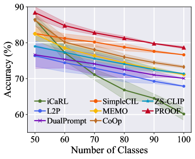
(a) CIFAR100 B50 Inc10

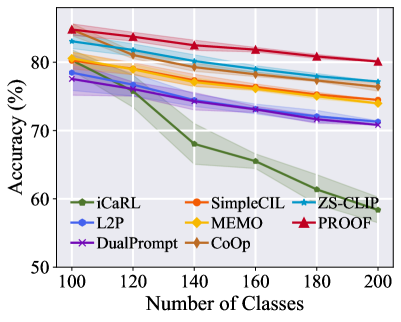
(b) ImageNet-R B100 Inc20

Figure 6: Results of multiple runs for CIFAR100 and ImageNet-R. The solid line represents the mean performance, while the shaded area indicates the standard deviation. Proof consistently and robustly outperforms other methods by a substantial margin.

B.1 Multiple Runs

Following [47], we conduct typical CIL comparisons by randomly splitting the classes with a fixed seed of 1993, and these results are reported in the main paper. In this supplementary section, we perform multiple runs by varying the random seed among {$1993,1994,1995,1996,1997$}. We repeat the comparison on CIFAR100 Base50 Inc10 and ImageNet-R Base100 Inc20 five times and present the results in Figure 6. The solid line represents the mean performance, while the shaded area indicates the standard deviation. From these figures, it is evident that Proof consistently outperforms other methods by a significant margin across different dataset splits. These results validate the robustness of Proof.

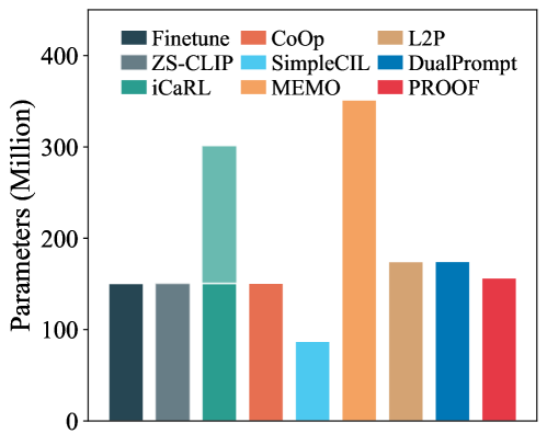
Figure 7: Number of parameters in different methods. The shaded area represents the parameters used during training but dropped during inference. Proof achieves state-of-the-art performance with a comparable number of parameters to other methods.

B.2 Parameter Analysis

As mentioned in the main paper, the additional parameters in Proof come from two sources: the projections and the fusion module. The projection layers are implemented with a single linear layer, each containing $d\times d$ parameters, where $d=512$ is the embedding dimension. Similarly, the cross-modal fusion is implemented with a single-head self-attention mechanism, and the number of parameters is determined by the weight matrices $W_{Q}$, $W_{K}$, and $W_{V}$, each containing $d\times d$ parameters. These extra parameters are negligible compared to the large backbone of the pre-trained CLIP model, which has approximately 150 million parameters.

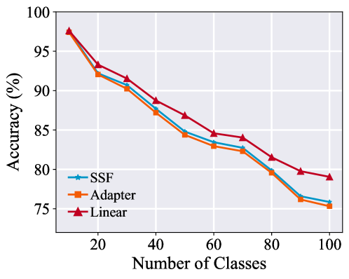
Figure 8: Variations of projection layers. The choice of using a single linear layer as the projection layer achieves the best performance.

To provide a clear comparison of the parameter numbers for each method, we present the details in Figure 7 using CIFAR100 B0 Inc10 as an example. The figure illustrates that Proof has a similar parameter scale to other finetune-based methods, while achieving significantly stronger performance. SimpleCIL, which only utilizes the vision branch, requires fewer parameters for the textual branch but lacks the zero-shot capability. L2P and DualPrompt also only require the vision branch but need an additional encoder to identify the appropriate prompt, resulting in a higher parameter count compared to Proof.

B.3 Variation of Projection Types

Apart from simple linear layers, there are other methods to implement the projection layers, such as layer-wise rescale (SSF) [34] and Adapter [23]. SSF learns a $d$-dimensional rescale parameter to project the features, while Adapter learns both the down-projection and up-projection for feature mapping. In this section, we explore the performance of these projection methods on CIFAR100 B0 Inc10 and present the results in Figure 8. The figure clearly demonstrates that using a single linear layer as the projection layer achieves the best performance among all methods, indicating its superiority. Furthermore, this result suggests that a simple linear mapping can effectively bridge the gap between visual and textual domains.

B.4 Variation of Context Information

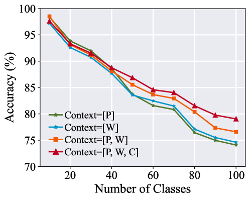
Figure 9: Variations of context information. The choice of using visual prototypes, textual prototypes, and context prompts as the context information achieves the best performance.

In the main paper, we discuss the composition of the context information $\mathbf{Context}$, which should include information from visual prototypes, textual classifiers, and context prompts. In this section, we conduct ablations to demonstrate the effectiveness of constructing $\mathbf{Context}$ with $[\mathbf{P},\mathbf{W},\mathbf{C}]$. Specifically, we perform experiments on CIFAR100 B0 Inc10 and change the context construction to $\mathbf{Context}=\mathbf{P}$ (visual prototypes only), $\mathbf{Context}=\mathbf{W}$ (textual prototypes only), $\mathbf{Context}=[\mathbf{P},\mathbf{W}]$ (visual and textual prototypes), and $\mathbf{Context}=[\mathbf{P},\mathbf{W},\mathbf{C}]$ (current choice). We keep the same classification rule for these ablations, i.e., classification via Eq. 9. When visual/textual prototypes are not included in the context, we use the projected features without adaptation as the matching target in Eq. 8. The results are presented in Figure 9.

From the results, we observe that using visual prototypes or textual prototypes alone yields similar performance, and the impact of adjustment is marginal. However, when both visual and textual prototypes are jointly utilized as context information, the model can learn from cross-modality and achieve better performance. Lastly, the introduction of context prompts into the context further enhances the performance of Proof, resulting in the best performance among all variations.

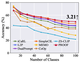
(a) Aircraft Base0 Inc10

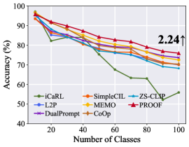
(b) CIFAR100 Base0 Inc10

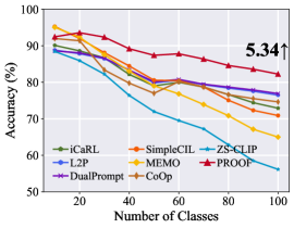
(c) Cars Base0 Inc10

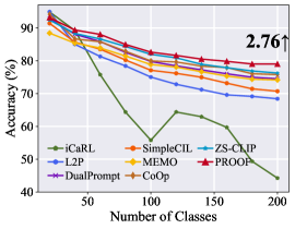
(d) ImageNet-R Base0 Inc20

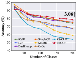
(e) CUB Base0 Inc20

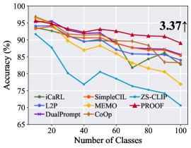
(f) UCF Base0 Inc10

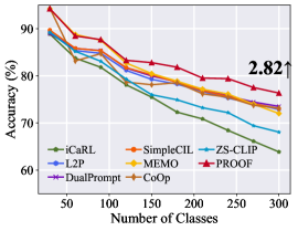
(g) SUN Base0 Inc30

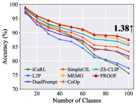
(h) Food Base0 Inc10

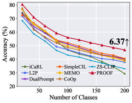
(i) ObjectNet Base0 Inc20

Figure 10: Incremental performance of different methods when using OpenAI weights. We report the performance gap after the last incremental stage of Proof and the runner-up method at the end of the line. Proof consistently achieves the best performance regardless of the pre-trained weights used.

B.5 Different Pre-trained Weights

In the main paper, we discussed two popular weights for pre-trained CLIP: OpenAI [46] and OpenCLIP [24]. We primarily presented the results of the OpenCLIP pre-trained model in the main paper, while providing the results of the OpenAI weights using a radar chart. In this section, we present the full results of the OpenAI pre-trained CLIP on nine benchmark datasets in Figure 10. The results demonstrate that Proof consistently achieves the best performance among all methods, regardless of the pre-trained weights used. This highlights the robustness of Proof in the learning process.

B.6 Full Results

We provide the complete results of the benchmark comparison in the main paper, which are presented in Table 2 and Figures 11 and 12. These results are obtained using OpenCLIP pre-trained weights on LAION-400M [24]. Table 2 displays the average and last accuracy for the nine benchmark datasets. Figures 11 and 12 illustrate the incremental performance with varying numbers of base classes. Across all these evaluations, Proof consistently outperforms the compared methods, demonstrating its superior performance.

Table 2: Average and last performance comparison of different methods. The first and second columns represent the methods with and without exemplars. The performance of L2P and DualPrompt are reproduced with the source code with exemplars. The best performance is shown in bold.

Method	Exemplar	Aircraft				CIFAR100				Cars
		B0 Inc10		B50 Inc10		B0 Inc10		B50 Inc10		B0 Inc10		B50 Inc10
		$\bar{\mathcal{A}}$	${\mathcal{A}_{B}}$	$\bar{\mathcal{A}}$	${\mathcal{A}_{B}}$	$\bar{\mathcal{A}}$	${\mathcal{A}_{B}}$	$\bar{\mathcal{A}}$	${\mathcal{A}_{B}}$	$\bar{\mathcal{A}}$	${\mathcal{A}_{B}}$	$\bar{\mathcal{A}}$	${\mathcal{A}_{B}}$
Finetune	✗	3.16	0.96	1.72	1.05	7.84	4.44	5.30	2.46	3.14	1.10	1.54	1.13
Finetune LiT [75]	✗	27.74	14.28	25.10	13.77	44.66	14.69	27.69	7.67	84.12	72.37	83.08	78.23
Finetune CoOp [85]	✗	14.54	7.14	13.05	7.77	47.00	24.24	41.23	24.12	36.46	21.65	37.40	20.87
SimpleCIL [83]	✗	59.24	48.09	53.05	48.09	84.15	76.63	80.20	76.63	92.04	86.85	88.96	86.85
ZS-CLIP [46]	✗	26.66	17.22	21.70	17.22	81.81	71.38	76.49	71.38	82.60	76.37	78.32	76.37
CoOp [85]	✓	44.26	39.87	41.81	39.18	83.37	73.36	78.34	73.04	89.73	84.91	87.98	86.60
iCaRL [47]	✓	53.60	43.98	50.40	45.33	79.91	63.94	71.94	63.00	89.38	84.95	86.71	84.19
MEMO [82]	✓	42.24	25.41	38.16	27.75	84.67	74.98	80.75	75.34	88.23	81.31	84.90	81.83
L2P [64]	✓	55.06	44.88	47.78	43.37	76.42	66.21	72.67	67.88	83.81	72.44	79.76	73.47
DualPrompt [63]	✓	55.95	46.53	50.93	46.50	79.07	70.06	74.81	70.75	85.30	74.35	81.32	75.85
Proof	✓	61.00	53.59	59.99	58.90	86.70	79.05	82.92	78.87	93.26	89.84	90.53	89.54

Method	Exemplar	ImageNet-R				CUB				UCF
		B0 Inc20		B100 Inc20		B0 Inc20		B100 Inc20		B0 Inc10		B50 Inc10
		$\bar{\mathcal{A}}$	${\mathcal{A}_{B}}$	$\bar{\mathcal{A}}$	${\mathcal{A}_{B}}$	$\bar{\mathcal{A}}$	${\mathcal{A}_{B}}$	$\bar{\mathcal{A}}$	${\mathcal{A}_{B}}$	$\bar{\mathcal{A}}$	${\mathcal{A}_{B}}$	$\bar{\mathcal{A}}$	${\mathcal{A}_{B}}$
Finetune	✗	1.37	0.43	1.01	0.88	2.06	0.64	0.56	0.47	4.51	1.59	1.21	0.80
Finetune LiT [75]	✗	64.88	30.42	57.75	29.77	58.15	35.28	51.95	35.96	79.25	64.84	81.79	65.40
Finetune CoOp [85]	✗	60.73	37.52	54.20	39.77	27.61	8.57	24.03	10.14	47.85	33.46	42.02	24.74
SimpleCIL [83]	✗	81.06	74.48	76.84	74.48	83.81	77.52	79.75	77.52	90.44	85.68	88.12	85.68
ZS-CLIP [46]	✗	83.37	77.17	79.57	77.17	74.38	63.06	67.96	63.06	75.50	67.64	71.44	67.64
CoOp [85]	✓	82.40	76.20	79.76	77.13	77.34	68.70	74.09	67.47	90.13	86.24	88.36	85.71
iCaRL [47]	✓	72.22	54.38	68.67	60.15	82.04	74.74	78.57	75.07	89.47	84.34	88.51	84.11
MEMO [82]	✓	80.00	74.07	76.72	73.95	77.32	65.69	72.88	66.41	84.02	74.08	82.58	75.48
L2P [64]	✓	75.73	67.22	74.15	71.20	79.23	68.54	75.85	71.12	88.71	83.93	86.51	83.22
DualPrompt [63]	✓	78.47	70.82	72.98	69.18	83.21	74.94	78.06	74.27	89.48	85.41	86.96	84.65
Proof	✓	85.34	80.10	82.32	80.30	84.93	79.43	81.67	79.18	92.34	89.92	91.70	89.16

Method	Exemplar	SUN				Food				ObjectNet
		B0 Inc30		B150 Inc30		B0 Inc10		B50 Inc10		B0 Inc20		B100 Inc20
		$\bar{\mathcal{A}}$	${\mathcal{A}_{B}}$	$\bar{\mathcal{A}}$	${\mathcal{A}_{B}}$	$\bar{\mathcal{A}}$	${\mathcal{A}_{B}}$	$\bar{\mathcal{A}}$	${\mathcal{A}_{B}}$	$\bar{\mathcal{A}}$	${\mathcal{A}_{B}}$	$\bar{\mathcal{A}}$	${\mathcal{A}_{B}}$
Finetune	✗	4.51	1.59	0.78	0.72	3.49	1.71	2.14	1.52	1.34	0.47	0.69	0.54
Finetune LiT [75]	✗	79.25	64.84	38.23	20.00	40.62	12.96	29.74	12.05	43.27	17.46	32.85	17.17
Finetune CoOp [85]	✗	45.93	23.11	39.33	24.89	36.01	14.18	33.13	18.67	21.24	6.29	16.21	6.82
SimpleCIL [83]	✗	82.13	75.58	78.62	75.58	87.89	81.65	84.73	81.65	52.06	40.13	45.11	40.13
ZS-CLIP [46]	✗	79.42	72.11	74.95	72.11	87.86	81.92	84.75	81.92	38.43	26.43	31.12	26.43
CoOp [85]	✓	80.46	73.44	77.68	73.06	85.38	76.15	81.74	76.35	46.16	33.81	40.40	34.47
iCaRL [47]	✓	78.56	67.30	74.74	69.07	84.12	71.68	78.86	70.64	45.28	26.97	37.22	26.15
MEMO [82]	✓	81.48	73.45	78.00	73.87	89.18	82.85	86.50	83.08	46.98	33.37	41.62	34.67
L2P [64]	✓	79.83	72.14	76.16	72.32	84.48	75.22	85.04	80.56	46.18	34.00	43.90	39.57
DualPrompt [63]	✓	80.14	73.06	77.25	73.82	87.12	81.27	85.37	82.36	53.13	40.59	45.84	40.37
Proof	✓	83.57	77.28	80.70	77.49	90.04	84.73	87.52	84.74	55.28	44.36	49.64	43.65

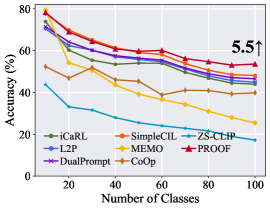
(a) Aircraft Base0 Inc10

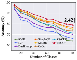
(b) CIFAR100 Base0 Inc10

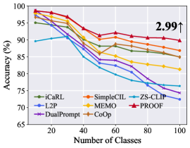
(c) Cars Base0 Inc10

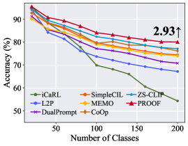
(d) ImageNet-R Base0 Inc20

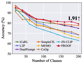
(e) CUB Base0 Inc20

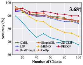
(f) UCF Base0 Inc10

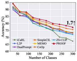
(g) SUN Base0 Inc30

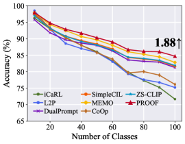
(h) Food Base0 Inc10

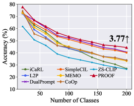
(i) ObjectNet Base0 Inc20

Figure 11: Incremental performance of different methods. We report the performance gap after the last incremental stage of Proof and the runner-up method at the end of the line.

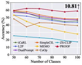
(a) Aircraft Base50 Inc10

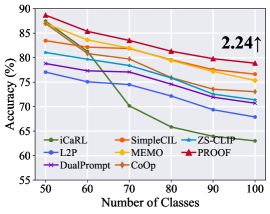
(b) CIFAR100 Base50 Inc10

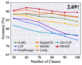
(c) Cars Base50 Inc10

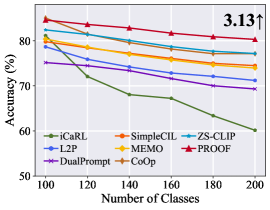
(d) ImageNet-R Base100 Inc20

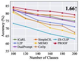
(e) CUB Base100 Inc20

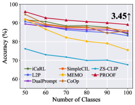
(f) UCF Base50 Inc10

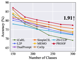
(g) SUN Base150 Inc30

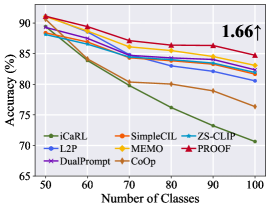
(h) Food Base50 Inc10

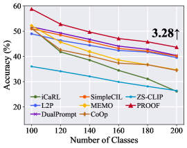
(i) ObjectNet Base100 Inc20

Figure 12: Incremental performance of different methods with large base classes. We report the performance gap after the last incremental stage of Proof and the runner-up method at the end of the line.

C Experimental Details

This section provides detailed information about the experiments conducted, including the introduction of datasets, exemplar selection, and the methods compared in the paper.

C.1 Dataset Introduction

In our evaluation, we utilize nine datasets, which are introduced in Table 3 in the main paper. It is worth noting that some of these datasets have a larger number of classes, but we select a subset of classes for ease of data split and evaluation.

Exemplar Selection: As mentioned in the main paper, we follow the exemplar selection approach in [47, 67, 22] to utilize herding algorithm [65]. In addition, there are two typical methods [81] to store these exemplars in memory.

1. Fixed Memory Budget: In this approach, a fixed memory budget of $K$ instances is allocated. Given the number of seen classes denoted as $|\mathcal{Y}_{b}|$, the model selects $\frac{K}{|\mathcal{Y}_{b}|}$ exemplars per class after each incremental stage.

2. Expandable Exemplar Set: In this method, an expandable exemplar set is maintained as the data evolves. With the number of exemplars per class denoted as $k$, the model stores $|\mathcal{Y}_{b}|\times k$ exemplars in total after each incremental stage.

We evaluate both protocols using these benchmark datasets in our experiments. Specifically, we employ the first policy for CIFAR100 and Food, keeping a total of 2,000 exemplars. Since these datasets consist of 100 classes, the average number of exemplars per class after the last incremental stage is 20. We adopt the second policy for the other datasets and store 20 exemplars per class.

Table 3: Introduction about benchmark datasets.

Dataset	# training instances	# testing instances	# Classes	Link
CIFAR100	50,000	10,000	100	Link
CUB200	9,430	2,358	200	Link
ImageNet-R	24,000	6,000	200	Link
ObjectNet	26,509	6,628	200	Link
Aircraft	6,667	3,333	100	Link
Cars	4,135	4,083	100	Link
UCF	10,053	2,639	100	Link
SUN	72,870	18,179	300	Link
Food	79,998	20,012	100	Link

C.2 Compared methods introduction

This section provides an overview of the compared methods discussed in the main paper. These methods, listed in the order presented in Table 2, include:

• Finetune: This baseline method involves finetuning the pre-trained CLIP model using contrastive loss. No regularization terms are set, and no part of the model is frozen, allowing us to observe the forgetting phenomenon in sequential learning.

• Finetune LiT [75]: Following LiT, which freezes the image encoder and only finetunes the text encoder, we design Finetune LiT with CIL. Similar to finetune, we sequentially tune the model with contrastive loss while the image encoder is frozen during optimization.

• Finetune CoOp [85]: Following the CoOp method, this approach freezes both the image encoder and text encoder. It optimizes a learnable prompt tensor $\mathbf{t}$ (as in Eq.4) using contrastive loss without utilizing any historical data for rehearsal.

• SimpleCIL [83]: This method relies on the pre-trained image encoder and does not involve the text encoder. The frozen image encoder extracts class centers (prototypes) for each new class, and a cosine classifier is utilized for classification. Since the model is not updated via backpropagation, it showcases the generalizability of the pre-trained vision encoder on downstream tasks.

• ZS-CLIP [46]: This baseline freezes the pre-trained CLIP model and predicts the logits of each incoming class using cosine similarity (Eq. 2). It serves as a reference for the performance of pre-trained CLIP on downstream tasks.

• CoOp (with exemplars): This method combines the CoOp approach with exemplar rehearsal. During the learning of new classes, the model utilizes a combination of the current dataset and exemplar set to optimize the learnable prompt.

• iCaRL [47]: iCaRL is a typical class-incremental learning algorithm that employs knowledge distillation and exemplar replay to mitigate forgetting. It combines contrastive loss with distillation loss to learn new classes while retaining knowledge of old classes.

• MEMO [82]: As a state-of-the-art class-incremental learning algorithm based on network expansion, MEMO is modified to be compatible with the CLIP structure. The image and text encoders are expanded for new tasks, and the concatenated features are used for prediction based on cosine similarity.

• L2P [64]: L2P is a state-of-the-art class-incremental learning algorithm utilizing pre-trained vision transformers. In this case, the text encoder of CLIP is dropped, and a prompt pool (as in Eq. 3) is learned to adapt to evolving data. Another pre-trained image encoder is required to select the appropriate prompt during inference.

• DualPrompt [63]: DualPrompt is an extension of L2P that incorporates two types of prompts: general prompts and expert prompts. It also relies on another pre-trained image encoder for prompt retrieval.

It is important to note that these methods are compared fairly, meaning they are initialized with the same pre-trained weights for incremental learning. Since some compared methods are not designed with the CLIP encoder, we modify their backbone into pre-trained CLIP for a fair comparison. We use the same number of exemplars for a fair comparison of the methods with exemplars.

D Broader Impacts

In this work, we address the class-incremental learning problem with vision-language models, which is a fundamental challenge in machine learning. Our focus is on tackling the forgetting problem that arises when sequentially finetuning a vision-language model. We propose solutions to project and integrate features from multiple modalities for unified classification. Our research provides valuable insights for applications that struggle with managing the forgetting issue in large pre-trained vision-language models. However, there are still ample opportunities for further exploration in this field. Therefore, we aspire to stimulate discussions on class-incremental learning in real-world scenarios and encourage more research to develop practical models for this purpose.

We also acknowledge the ethical considerations associated with this technology. It is crucial to recognize that individuals expect learning systems to refrain from storing any personal information for future rehearsal. While there are risks involved in AI research of this nature, we believe that developing and demonstrating such techniques are vital for comprehending both the beneficial and potentially concerning applications of this technology. Our aim is to foster discussions regarding best practices and controls surrounding these methods, promoting responsible and ethical utilization of technology.

References

- [1] Jean-Baptiste Alayrac, Jeff Donahue, Pauline Luc, Antoine Miech, Iain Barr, Yana Hasson, Karel Lenc, Arthur Mensch, Katherine Millican, Malcolm Reynolds, et al. Flamingo: a visual language model for few-shot learning. NeurIPS, 35:23716–23736, 2022.
- [2] Rahaf Aljundi, Francesca Babiloni, Mohamed Elhoseiny, Marcus Rohrbach, and Tinne Tuytelaars. Memory aware synapses: Learning what (not) to forget. In ECCV, pages 139–154, 2018.
- [3] Rahaf Aljundi, Klaas Kelchtermans, and Tinne Tuytelaars. Task-free continual learning. In CVPR, pages 11254–11263, 2019.
- [4] Rahaf Aljundi, Min Lin, Baptiste Goujaud, and Yoshua Bengio. Gradient based sample selection for online continual learning. In NeurIPS, pages 11816–11825, 2019.
- [5] Stanislaw Antol, Aishwarya Agrawal, Jiasen Lu, Margaret Mitchell, Dhruv Batra, C Lawrence Zitnick, and Devi Parikh. Vqa: Visual question answering. In ICCV, pages 2425–2433, 2015.
- [6] Andrei Barbu, David Mayo, Julian Alverio, William Luo, Christopher Wang, Dan Gutfreund, Josh Tenenbaum, and Boris Katz. Objectnet: A large-scale bias-controlled dataset for pushing the limits of object recognition models. NeurIPS, 32, 2019.
- [7] Lukas Bossard, Matthieu Guillaumin, and Luc Van Gool. Food-101–mining discriminative components with random forests. In ECCV, pages 446–461. Springer, 2014.
- [8] Arslan Chaudhry, Puneet K Dokania, Thalaiyasingam Ajanthan, and Philip HS Torr. Riemannian walk for incremental learning: Understanding forgetting and intransigence. In ECCV, pages 532–547, 2018.
- [9] Arslan Chaudhry, Marc’Aurelio Ranzato, Marcus Rohrbach, and Mohamed Elhoseiny. Efficient lifelong learning with a-gem. In ICLR, 2018.
- [10] Guangyi Chen, Weiran Yao, Xiangchen Song, Xinyue Li, Yongming Rao, and Kun Zhang. Plot: Prompt learning with optimal transport for vision-language models. In ICLR, 2023.
- [11] Shoufa Chen, GE Chongjian, Zhan Tong, Jiangliu Wang, Yibing Song, Jue Wang, and Ping Luo. Adaptformer: Adapting vision transformers for scalable visual recognition. In NeurIPS, 2022.
- [12] Jia Deng, Wei Dong, Richard Socher, Li-Jia Li, Kai Li, and Li Fei-Fei. Imagenet: A large-scale hierarchical image database. In CVPR, pages 248–255, 2009.
- [13] Alexey Dosovitskiy, Lucas Beyer, Alexander Kolesnikov, Dirk Weissenborn, Xiaohua Zhai, Thomas Unterthiner, Mostafa Dehghani, Matthias Minderer, Georg Heigold, Sylvain Gelly, et al. An image is worth 16x16 words: Transformers for image recognition at scale. In ICLR, 2020.
- [14] Arthur Douillard, Matthieu Cord, Charles Ollion, Thomas Robert, and Eduardo Valle. Podnet: Pooled outputs distillation for small-tasks incremental learning. In ECCV, pages 86–102, 2020.
- [15] Arthur Douillard, Alexandre Ramé, Guillaume Couairon, and Matthieu Cord. Dytox: Transformers for continual learning with dynamic token expansion. In CVPR, pages 9285–9295, 2022.
- [16] Robert M French. Catastrophic forgetting in connectionist networks. Trends in cognitive sciences, 3(4):128–135, 1999.
- [17] Peng Gao, Shijie Geng, Renrui Zhang, Teli Ma, Rongyao Fang, Yongfeng Zhang, Hongsheng Li, and Yu Qiao. Clip-adapter: Better vision-language models with feature adapters. arXiv preprint arXiv:2110.04544, 2021.
- [18] Chuanxing Geng, Sheng-jun Huang, and Songcan Chen. Recent advances in open set recognition: A survey. IEEE transactions on pattern analysis and machine intelligence, 43(10):3614–3631, 2020.
- [19] Heitor Murilo Gomes, Jean Paul Barddal, Fabrício Enembreck, and Albert Bifet. A survey on ensemble learning for data stream classification. CSUR, 50(2):1–36, 2017.
- [20] Xu Han, Zhengyan Zhang, Ning Ding, Yuxian Gu, Xiao Liu, Yuqi Huo, Jiezhong Qiu, Yuan Yao, Ao Zhang, Liang Zhang, et al. Pre-trained models: Past, present and future. AI Open, 2:225–250, 2021.
- [21] Saihui Hou, Xinyu Pan, Chen Change Loy, Zilei Wang, and Dahua Lin. Lifelong learning via progressive distillation and retrospection. In ECCV, pages 437–452, 2018.
- [22] Saihui Hou, Xinyu Pan, Chen Change Loy, Zilei Wang, and Dahua Lin. Learning a unified classifier incrementally via rebalancing. In CVPR, pages 831–839, 2019.
- [23] Neil Houlsby, Andrei Giurgiu, Stanislaw Jastrzebski, Bruna Morrone, Quentin De Laroussilhe, Andrea Gesmundo, Mona Attariyan, and Sylvain Gelly. Parameter-efficient transfer learning for nlp. In ICML, pages 2790–2799, 2019.
- [24] Gabriel Ilharco, Mitchell Wortsman, Ross Wightman, Cade Gordon, Nicholas Carlini, Rohan Taori, Achal Dave, Vaishaal Shankar, Hongseok Namkoong, John Miller, Hannaneh Hajishirzi, Ali Farhadi, and Ludwig Schmidt. Openclip, July 2021.
- [25] Chao Jia, Yinfei Yang, Ye Xia, Yi-Ting Chen, Zarana Parekh, Hieu Pham, Quoc Le, Yun-Hsuan Sung, Zhen Li, and Tom Duerig. Scaling up visual and vision-language representation learning with noisy text supervision. In ICML, pages 4904–4916. PMLR, 2021.
- [26] Menglin Jia, Luming Tang, Bor-Chun Chen, Claire Cardie, Serge J. Belongie, Bharath Hariharan, and Ser-Nam Lim. Visual prompt tuning. In ECCV, pages 709–727. Springer, 2022.
- [27] James Kirkpatrick, Razvan Pascanu, Neil Rabinowitz, Joel Veness, Guillaume Desjardins, Andrei A Rusu, Kieran Milan, John Quan, Tiago Ramalho, Agnieszka Grabska-Barwinska, et al. Overcoming catastrophic forgetting in neural networks. PNAS, 114(13):3521–3526, 2017.
- [28] Jonathan Krause, Michael Stark, Jia Deng, and Li Fei-Fei. 3d object representations for fine-grained categorization. In ICCV Workshop, pages 554–561, 2013.
- [29] Alex Krizhevsky, Geoffrey Hinton, et al. Learning multiple layers of features from tiny images. Technical report, 2009.
- [30] Kuan-Ying Lee, Yuanyi Zhong, and Yu-Xiong Wang. Do pre-trained models benefit equally in continual learning? In WACV, pages 6485–6493, 2023.
- [31] Junnan Li, Dongxu Li, Silvio Savarese, and Steven Hoi. Blip-2: Bootstrapping language-image pre-training with frozen image encoders and large language models. arXiv preprint arXiv:2301.12597, 2023.
- [32] Xiang Lisa Li and Percy Liang. Prefix-tuning: Optimizing continuous prompts for generation. In ACL, pages 4582–4597, 2021.
- [33] Zhizhong Li and Derek Hoiem. Learning without forgetting. In ECCV, pages 614–629. Springer, 2016.
- [34] Dongze Lian, Zhou Daquan, Jiashi Feng, and Xinchao Wang. Scaling & shifting your features: A new baseline for efficient model tuning. In NeurIPS, 2022.
- [35] Victor Weixin Liang, Yuhui Zhang, Yongchan Kwon, Serena Yeung, and James Y Zou. Mind the gap: Understanding the modality gap in multi-modal contrastive representation learning. NeurIPS, 35:17612–17625, 2022.
- [36] Zhouhan Lin, Minwei Feng, Cicero Nogueira dos Santos, Mo Yu, Bing Xiang, Bowen Zhou, and Yoshua Bengio. A structured self-attentive sentence embedding. arXiv preprint arXiv:1703.03130, 2017.
- [37] Yaoyao Liu, Bernt Schiele, and Qianru Sun. Rmm: Reinforced memory management for class-incremental learning. NeurIPS, 34, 2021.
- [38] Yaoyao Liu, Yuting Su, An-An Liu, Bernt Schiele, and Qianru Sun. Mnemonics training: Multi-class incremental learning without forgetting. In CVPR, pages 12245–12254, 2020.
- [39] Yuning Lu, Jianzhuang Liu, Yonggang Zhang, Yajing Liu, and Xinmei Tian. Prompt distribution learning. In CVPR, pages 5206–5215, 2022.
- [40] Zilin Luo, Yaoyao Liu, Bernt Schiele, and Qianru Sun. Class-incremental exemplar compression for class-incremental learning. arXiv preprint arXiv:2303.14042, 2023.
- [41] Subhransu Maji, Esa Rahtu, Juho Kannala, Matthew Blaschko, and Andrea Vedaldi. Fine-grained visual classification of aircraft. arXiv preprint arXiv:1306.5151, 2013.
- [42] Chengzhi Mao, Revant Teotia, Amrutha Sundar, Sachit Menon, Junfeng Yang, Xin Wang, and Carl Vondrick. Doubly right object recognition: A why prompt for visual rationales. arXiv preprint arXiv:2212.06202, 2022.
- [43] Norman Mu, Alexander Kirillov, David Wagner, and Saining Xie. Slip: Self-supervision meets language-image pre-training. In ECCV, pages 529–544. Springer, 2022.
- [44] Adam Paszke, Sam Gross, Francisco Massa, Adam Lerer, James Bradbury, Gregory Chanan, Trevor Killeen, Zeming Lin, Natalia Gimelshein, Luca Antiga, et al. Pytorch: An imperative style, high-performance deep learning library. In NeurIPS, pages 8026–8037, 2019.
- [45] Bryan A Plummer, Liwei Wang, Chris M Cervantes, Juan C Caicedo, Julia Hockenmaier, and Svetlana Lazebnik. Flickr30k entities: Collecting region-to-phrase correspondences for richer image-to-sentence models. In ICCV, pages 2641–2649, 2015.
- [46] Alec Radford, Jong Wook Kim, Chris Hallacy, Aditya Ramesh, Gabriel Goh, Sandhini Agarwal, Girish Sastry, Amanda Askell, Pamela Mishkin, Jack Clark, et al. Learning transferable visual models from natural language supervision. In ICML, pages 8748–8763. PMLR, 2021.
- [47] Sylvestre-Alvise Rebuffi, Alexander Kolesnikov, Georg Sperl, and Christoph H Lampert. icarl: Incremental classifier and representation learning. In CVPR, pages 2001–2010, 2017.
- [48] Christoph Schuhmann, Richard Vencu, Romain Beaumont, Robert Kaczmarczyk, Clayton Mullis, Aarush Katta, Theo Coombes, Jenia Jitsev, and Aran Komatsuzaki. Laion-400m: Open dataset of clip-filtered 400 million image-text pairs. arXiv preprint arXiv:2111.02114, 2021.
- [49] James Seale Smith, Leonid Karlinsky, Vyshnavi Gutta, Paola Cascante-Bonilla, Donghyun Kim, Assaf Arbelle, Rameswar Panda, Rogerio Feris, and Zsolt Kira. Coda-prompt: Continual decomposed attention-based prompting for rehearsal-free continual learning. arXiv e-prints, pages arXiv–2211, 2022.
- [50] Yujun Shi, Kuangqi Zhou, Jian Liang, Zihang Jiang, Jiashi Feng, Philip HS Torr, Song Bai, and Vincent YF Tan. Mimicking the oracle: An initial phase decorrelation approach for class incremental learning. In CVPR, pages 16722–16731, 2022.
- [51] Jake Snell, Kevin Swersky, and Richard Zemel. Prototypical networks for few-shot learning. In NIPS, pages 4080–4090, 2017.
- [52] Khurram Soomro, Amir Roshan Zamir, and Mubarak Shah. Ucf101: A dataset of 101 human actions classes from videos in the wild. arXiv preprint arXiv:1212.0402, 2012.
- [53] Qing Sun, Fan Lyu, Fanhua Shang, Wei Feng, and Liang Wan. Exploring example influence in continual learning. In NeurIPS, 2022.
- [54] Michael Tschannen, Basil Mustafa, and Neil Houlsby. Image-and-language understanding from pixels only. arXiv preprint arXiv:2212.08045, 2022.
- [55] Ashish Vaswani, Noam Shazeer, Niki Parmar, Jakob Uszkoreit, Llion Jones, Aidan N Gomez, Łukasz Kaiser, and Illia Polosukhin. Attention is all you need. In NIPS, pages 5998–6008, 2017.
- [56] Oriol Vinyals, Alexander Toshev, Samy Bengio, and Dumitru Erhan. Show and tell: A neural image caption generator. In CVPR, pages 3156–3164, 2015.
- [57] C. Wah, S. Branson, P. Welinder, P. Perona, and S. Belongie. The Caltech-UCSD Birds-200-2011 Dataset. Technical Report CNS-TR-2011-001, California Institute of Technology, 2011.
- [58] Fu-Yun Wang, Da-Wei Zhou, Liu Liu, Han-Jia Ye, Yatao Bian, De-Chuan Zhan, and Peilin Zhao. BEEF: Bi-compatible class-incremental learning via energy-based expansion and fusion. In ICLR, 2023.
- [59] Fu-Yun Wang, Da-Wei Zhou, Han-Jia Ye, and De-Chuan Zhan. Foster: Feature boosting and compression for class-incremental learning. In ECCV, pages 398–414, 2022.
- [60] Wenhui Wang, Hangbo Bao, Li Dong, Johan Bjorck, Zhiliang Peng, Qiang Liu, Kriti Aggarwal, Owais Khan Mohammed, Saksham Singhal, Subhojit Som, et al. Image as a foreign language: Beit pretraining for all vision and vision-language tasks. arXiv preprint arXiv:2208.10442, 2022.
- [61] Yabin Wang, Zhiwu Huang, and Xiaopeng Hong. S-prompts learning with pre-trained transformers: An occam’s razor for domain incremental learning. In NeurIPS, 2022.
- [62] Zifeng Wang, Zheng Zhan, Yifan Gong, Geng Yuan, Wei Niu, Tong Jian, Bin Ren, Stratis Ioannidis, Yanzhi Wang, and Jennifer Dy. Sparcl: Sparse continual learning on the edge. In NeurIPS, 2022.
- [63] Zifeng Wang, Zizhao Zhang, Sayna Ebrahimi, Ruoxi Sun, Han Zhang, Chen-Yu Lee, Xiaoqi Ren, Guolong Su, Vincent Perot, Jennifer Dy, et al. Dualprompt: Complementary prompting for rehearsal-free continual learning. In ECCV, pages 631–648, 2022.
- [64] Zifeng Wang, Zizhao Zhang, Chen-Yu Lee, Han Zhang, Ruoxi Sun, Xiaoqi Ren, Guolong Su, Vincent Perot, Jennifer Dy, and Tomas Pfister. Learning to prompt for continual learning. In CVPR, pages 139–149, 2022.
- [65] Max Welling. Herding dynamical weights to learn. In ICML, pages 1121–1128, 2009.
- [66] Mitchell Wortsman, Gabriel Ilharco, Jong Wook Kim, Mike Li, Simon Kornblith, Rebecca Roelofs, Raphael Gontijo Lopes, Hannaneh Hajishirzi, Ali Farhadi, Hongseok Namkoong, et al. Robust fine-tuning of zero-shot models. In CVPR, pages 7959–7971, 2022.
- [67] Yue Wu, Yinpeng Chen, Lijuan Wang, Yuancheng Ye, Zicheng Liu, Yandong Guo, and Yun Fu. Large scale incremental learning. In CVPR, pages 374–382, 2019.
- [68] Jianxiong Xiao, James Hays, Krista A Ehinger, Aude Oliva, and Antonio Torralba. Sun database: Large-scale scene recognition from abbey to zoo. In CVPR, pages 3485–3492. IEEE, 2010.
- [69] Shipeng Yan, Jiangwei Xie, and Xuming He. Der: Dynamically expandable representation for class incremental learning. In CVPR, pages 3014–3023, 2021.
- [70] Jiahui Yu, Zirui Wang, Vijay Vasudevan, Legg Yeung, Mojtaba Seyedhosseini, and Yonghui Wu. Coca: Contrastive captioners are image-text foundation models. arXiv preprint arXiv:2205.01917, 2022.
- [71] Lu Yu, Bartlomiej Twardowski, Xialei Liu, Luis Herranz, Kai Wang, Yongmei Cheng, Shangling Jui, and Joost van de Weijer. Semantic drift compensation for class-incremental learning. In CVPR, pages 6982–6991, 2020.
- [72] Tao Yu, Zhihe Lu, Xin Jin, Zhibo Chen, and Xinchao Wang. Task residual for tuning vision-language models. arXiv preprint arXiv:2211.10277, 2022.
- [73] Lu Yuan, Dongdong Chen, Yi-Ling Chen, Noel Codella, Xiyang Dai, Jianfeng Gao, Houdong Hu, Xuedong Huang, Boxin Li, Chunyuan Li, et al. Florence: A new foundation model for computer vision. arXiv preprint arXiv:2111.11432, 2021.
- [74] Friedemann Zenke, Ben Poole, and Surya Ganguli. Continual learning through synaptic intelligence. In ICML, pages 3987–3995, 2017.
- [75] Xiaohua Zhai, Xiao Wang, Basil Mustafa, Andreas Steiner, Daniel Keysers, Alexander Kolesnikov, and Lucas Beyer. Lit: Zero-shot transfer with locked-image text tuning. In CVPR, pages 18123–18133, 2022.
- [76] Renrui Zhang, Wei Zhang, Rongyao Fang, Peng Gao, Kunchang Li, Jifeng Dai, Yu Qiao, and Hongsheng Li. Tip-adapter: Training-free adaption of clip for few-shot classification. In ECCV, pages 493–510. Springer, 2022.
- [77] Yaqian Zhang, Bernhard Pfahringer, Eibe Frank, Albert Bifet, Nick Jin Sean Lim, and Alvin Jia. A simple but strong baseline for online continual learning: Repeated augmented rehearsal. In NeurIPS, 2022.
- [78] Bowen Zhao, Xi Xiao, Guojun Gan, Bin Zhang, and Shu-Tao Xia. Maintaining discrimination and fairness in class incremental learning. In CVPR, pages 13208–13217, 2020.
- [79] Hanbin Zhao, Yongjian Fu, Mintong Kang, Qi Tian, Fei Wu, and Xi Li. Mgsvf: Multi-grained slow vs. fast framework for few-shot class-incremental learning. IEEE Transactions on Pattern Analysis and Machine Intelligence, 2021.
- [80] Da-Wei Zhou, Fu-Yun Wang, Han-Jia Ye, and De-Chuan Zhan. Pycil: a python toolbox for class-incremental learning. SCIENCE CHINA Information Sciences, 66(9):197101–, 2023.
- [81] Da-Wei Zhou, Qi-Wei Wang, Zhi-Hong Qi, Han-Jia Ye, De-Chuan Zhan, and Ziwei Liu. Deep class-incremental learning: A survey. arXiv preprint arXiv:2302.03648, 2023.
- [82] Da-Wei Zhou, Qi-Wei Wang, Han-Jia Ye, and De-Chuan Zhan. A model or 603 exemplars: Towards memory-efficient class-incremental learning. In ICLR, 2023.
- [83] Da-Wei Zhou, Han-Jia Ye, De-Chuan Zhan, and Ziwei Liu. Revisiting class-incremental learning with pre-trained models: Generalizability and adaptivity are all you need. arXiv preprint arXiv:2303.07338, 2023.
- [84] Kaiyang Zhou, Jingkang Yang, Chen Change Loy, and Ziwei Liu. Conditional prompt learning for vision-language models. In CVPR, pages 16816–16825, 2022.
- [85] Kaiyang Zhou, Jingkang Yang, Chen Change Loy, and Ziwei Liu. Learning to prompt for vision-language models. International Journal of Computer Vision, 130(9):2337–2348, 2022.