Non-stationary Gaussian Process Surrogates

Abstract

We provide a survey of non-stationary surrogate models which utilize Gaussian processes (GPs) or variations thereof, including non-stationary kernel adaptations, partition and local GPs, and spatial warpings through deep Gaussian processes. We also overview publicly available software implementations and conclude with a bake-off involving an 8-dimensional satellite drag computer experiment. Code for this example is provided in a public git repository.

1 Introduction

Computer simulations are becoming increasingly relevant as methods of data collection, whether to augment or stand in place of actual physical observations, particularly when physical observations are too costly or impossible to come by. Such computer “experiments” pervade many scientific fields including aerospace engineering (e.g., Renganathan et al.,, 2021), cosmology (e.g., Moran et al.,, 2022), epidemiology (e.g., Andrianakis et al.,, 2015), biology (e.g., Johnson,, 2008), and physiology (e.g., Plumlee et al.,, 2016). Computer experiments aim to mimic the real-world. As they have been refined over the years, and their fidelity improved, they have increasingly required heftier computation. This limits the number of simulator evaluations that may be obtained, even with modern supercomputing resources. In such situations, a statistical “surrogate” model (also called an “emulator”), which is trained on a limited amount of simulation data, can be useful as a stand-in for additional expensive simulations. That is, as long as it can provide accurate predictions with appropriate uncertainty quantifiaction (UQ) at untried input configurations. Surrogates can be a crucial tool for turning limited computer simulation data into actionable scientific conclusions.

The stipulation we made above bears repeating; the usefulness of a surrogate relies on its ability to provide appropriate uncertainty quantification. UQ is a priority because surrogate models are most often tools to be used to another end: objectives we refer to as “downstream tasks.” For example, the objective may be to maximize the response, i.e., global optimization. Consider a simulation of a wind turbine in which input configurations include turbine height, angle, and blade dimensions. These affect the energy output of the turbine (e.g., Marten et al.,, 2013). A natural research objective is to find the configuration that maximizes energy output. Adaptive, sequential surrogate-based design targeting a global optimum is commonly termed Bayesian optimization (BO; Jones et al.,, 1998; Eriksson et al.,, 2019; Binois and Wycoff,, 2022). [Often, BO is used in machine learning to optimize settings of model hyperparameters.] In this endeavour, knowing where high outputs are found is just as important as identifying input regions of high uncertainty to explore further (striking a balance between exploitation and exploration). Another objective may be to ensure the system being simulated meets certain safety thresholds by quantifying the probability of a system failure. Consider a simulation of an aircraft whose response variable is the amount of aircraft vibration. It is dangerous for the vibrations to exceed certain safety levels; thus, the design objective is to identify the input regions that result in unsafe vibration conditions (e.g., Stanford et al.,, 2022) so they can be avoided in practice. Both these objectives fall under the umbrella of “sequential design” or “active learning,” in which input configurations are chosen sequentially and strategically to target specific learning outcomes based on surrogate information. Another common objective is simulator calibration, in which tuning parameters of the simulator are calibrated to real-world physical observations (Kennedy and O’Hagan,, 2001). Sequential design has also been entertained in calibration contexts (e.g., Koermer et al.,, 2023).

So, we need a statistical model that can handle the nonlinear response surfaces typical of computer simulations, work with limited training data, and provide accurate predictions with thorough UQ to facilitate downstream tasks. Piece of cake, right? The “go-to” surrogate model is a Gaussian process (GP). GPs are nonlinear, nonparametric regression models that are preferred for their predictive prowess; see Santner et al., (2018) and Gramacy, (2020) for reviews of GPs for surrogate modeling. While GPs are the canonical surrogate modeling choice, the computer experiment community is only one of three big players in the GP world. GPs are widely used in both spatial statistics (Banerjee et al.,, 2003; Stein,, 1999; Cressie,, 2015) and machine learning (ML; Rasmussen and Williams,, 2005). Although GPs unite these communities, there are subtle differences in applications which, naturally, inform modeling decisions. In spatial statistics, the focus is on low dimensional input spaces, often with missing data and anticipated measurement error. [GP regression is also called “kriging”, especially in a geospatial modeling context.] The norm in ML is high input dimension, large data sizes, and lots of noise. On the contrary, computer experiments commonly live in modest dimensional realms with little-to-no noise (though there are exceptions, e.g., Baker et al.,, 2022), and small-to-moderate data sizes due to hefty computational costs. Nevertheless, many of the key innovations for GP surrogate modeling arise from the spatial and ML communities. We will revisit this motif throughout this chapter.

Despite their nonlinear flexibility, traditional GPs are limited by the assumption of stationarity. Stationary GP modeling relies solely on pairwise distances between inputs, so they must impart similar dynamics across the entire input space (more on this in Section 2). Yet non-stationary response surfaces that exhibit regime shifts, sharp turns, and/or space-varying dynamics are common in computer experiments. For example, consider an aerospace simulation of a rocket re-entering the atmosphere (Pamadi et al.,, 2004), as featured in Gramacy, (2020, Chapter 2). A visual is provided later in Figure 2. There is an abrupt shift in aeronautical dynamics when speeds cross the sound barrier. A stationary GP is unable to accommodate the stark ridge in the response surface at this boundary. Alas, we are finally at the motivation behind this chapter: advancements to typical GP models that allow non-stationary flexibility without sacrificing predictive prowess or uncertainty quantification.

There has been much work on non-stationary GP modeling, with many contributions from spatial and ML communities. We see these methods falling into three categories:

• Non-stationary kernels: adapt the GP kernel formulation spatially so dynamics are no longer strictly a function of relative distance. These methods originate from spatial statistics, where the focus is on low input dimension.

• Divide-and-conquer: partition the input space and use traditional stationary GPs independently in each region. Localization is common in surrogate modeling and in geospatial contexts, but such schemes forfeit a degree of global scope when strong long-range dynamics are present.

• Spatial warping: nonlinearly map inputs so that the process can be depicted as plausibly stationary. The most recently popular of these these being the “deep Gaussian process” (DGP; Damianou and Lawrence,, 2013) which uses a stationary GP as the warping function. DGPs combine non-stationary and global modeling, albeit at the cost of some additional computation. Although this modern approach is inspired by recent advances in deep neural networks (DNNs) in machine learning, it actually originated in the spatial and computer modeling literature a decade before DNNs came on the scene.

In the remainder of this chapter, after a brief review of stationary GPs, we will address each of these three categories, keeping an eye on surrogate modeling applications and publicly available implementations.

2 Gaussian process fundamentals

Allow us to introduce GPs in their simplest form, to motivate the upgraded versions we will discuss later. Let $f:\mathbb{R}^{d}\rightarrow\mathbb{R}$ represent a black-box computer simulation. Denote a $d$-dimensional vectorized input configuration as $\mathbf{x}$, with corresponding simulator output $y=f(\mathbf{x})$. Similarly, let $X_{n}$ denote the row-combined matrix of $n$ input configurations with $\mathbf{y}_{n}=f(X_{n})$. A GP prior assumes a multivariate normal distribution over the response, $\mathbf{y}_{n}\sim N\left(\bm{\mu},\bm{\Sigma}(X_{n})\right)$. It is possible to model the prior mean as a linear combination of inputs, i.e., $\bm{\mu}=X_{n}\bm{\beta}$, but we will assume $\bm{\mu}=\mathbf{0}$, as is common after centering, without loss of generality. The prior covariance matrix $\bm{\Sigma}(X_{n})$ is an $n\times n$ matrix with elements $\bm{\Sigma}(X_{n})^{ij}=\Sigma(\mathbf{x}_{i},\mathbf{x}_{j})$ denoting the covariance between the $i^{th}$ and $j^{th}$ input locations.

A common choice for $\bm{\Sigma}(\cdot)$ is the Gaussian or squared exponential kernel,

$$\Sigma(\mathbf{x}_{i},\mathbf{x}_{j})=\Sigma(||\mathbf{x}_{i}-\mathbf{x}_{j}||)=\sigma^{2}\left(\mathrm{exp}\left(-\frac{||\mathbf{x}_{i}-\mathbf{x}_{j}||^{2}}{\phi}\right)+\nu\mathbb{I}_{i=j}\right),$$ (1)

where $\sigma^{2}$ acts as a scale parameter, $\phi$ is a lengthscale, and $\nu$ is a nugget/noise parameter. These parameters may be estimated through maximum likelihood estimation (as in Gramacy,, 2020) or sampled through Markov Chain Monte Carlo (MCMC; as in Sauer et al.,, 2023). In deterministic computer simulations, we often fix $\nu$ at a small constant, on the scale of $1\times 10^{-6}$. One may swap in a Matérn kernel (Stein,, 1999), parameterized similarly. These covariance functions are stationary as they are solely functions of relative distances. Even if we expand to separable vectorized lengthscales $\phi=[\phi_{1},\dots,\phi_{d}]$ (Gramacy,, 2020, Chapter 5), the kernels are unable to encode information aside from (possibly scaled) relative distances. This forces similar dynamics across the entire domain, i.e., stationarity.

Conditioned on observed training data, posterior predictions at $n_{p}$ input locations, $X_{p}$, follow

$$\mathbf{y}_{p}\mid X_{n},\mathbf{y}_{n}\sim N\left(\bm{\mu}^{\star},\bm{\Sigma}^{\star}\right)\quad\textrm{where}\quad\begin{array}[]{l}\bm{\mu}^{\star}=\bm{\Sigma}(X_{p},X_{n})\bm{\Sigma}(X_{n})^{-1}\mathbf{y}_{n}\\ \bm{\Sigma}^{\star}=\bm{\Sigma}(X_{p})-\bm{\Sigma}(X_{p},X_{n})\bm{\Sigma}(X_{n})^{-1}\bm{\Sigma}(X_{n},X_{p}),\end{array}$$ (2)

and $\bm{\Sigma}(X_{p},X_{n})$ is the $n_{p}\times n$ matrix containing the covariances between each row of $X_{p}$ and each row of $X_{n}$. These closed form analytic posterior moments are convenient, but they rely heavily on the choice of covariance kernel – notice how frequently $\bm{\Sigma}(\cdot)$ features in (2). If the kernel is an ill-fit for the response surface dynamics, GP predictions will be handicapped.

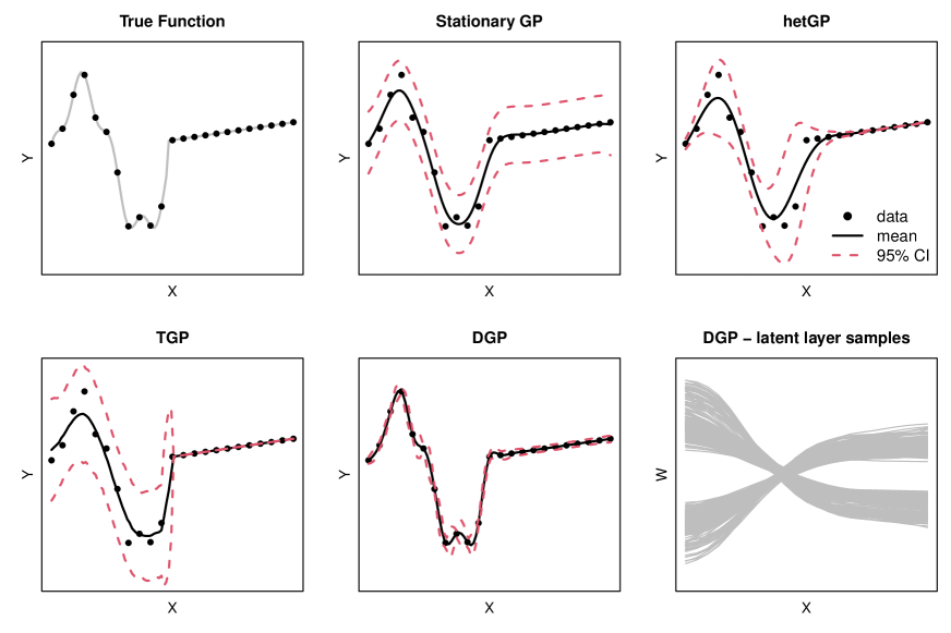
Figure 1: Various surrogate fits to the piecewise Higdon function. Training data is observed without noise, but each surrogate is tasked with learning the noise level. The lower right panel shows elliptical slice samples of the DGP’s latent layer, stretching inputs in the left region and compressing inputs in the right region.

For example, consider the non-stationary “Higdon function” generated piecewise following Gramacy et al., (2004), shown in the upper left panel of Figure 1. The left region is high signal, but the right region is far less interesting. Although the training data is observed without noise, we allow surrogates to estimate a global noise parameter – an additional test of surrogate proficiency in this setting. A stationary GP fit is provided in the upper middle panel. In trying to reconcile the disparate regimes, it over-smooths in the left region and over-inflates variance predictions in the right region. We shall revisit the other panels of the Figure in due course, after introducing recently popular forms of nonstationary modeling.

3 Non-stationary kernels

If a stationary covariance kernel is not an appropriate fit, a natural remedy is to change the kernel to one that is more flexible, while still maintaining positive definiteness. A non-stationary kernel $\bm{\Sigma}_{\mathrm{ns}}(\cdot)$ must rely on more than relative distances, i.e., $\bm{\Sigma}_{\mathrm{ns}}(\mathbf{x}_{i},\mathbf{x}_{j})\neq\bm{\Sigma}(||\mathbf{x}_{i}-\mathbf{x}_{j}||)$. This advancement requires introducing auxilary quantities into the covariance, which are typically unknown and ideally learned from training data.

Higdon et al., (1999) allowed for non-stationary kernels through process convolution, i.e., $\bm{\Sigma}_{\mathrm{ns}}(\mathbf{x}_{i},\mathbf{x}_{j})=\int k_{\mathbf{x}_{i}}(u)k_{\mathbf{x}_{j}}(u)du$ where $k_{\mathbf{x}_{i}}$ is a squared exponential kernel centered at $\mathbf{x}_{i}$. They utilized a hierarchical Bayesian framework and sampled unknown quantities through MCMC, allowing for full UQ. Paciorek and Schervish, (2003) later generalized this work to the class of Matérn kernels, with further development by Katzfuss, (2013). The use of process convolutions for non-stationary GP modeling is popular and has recent use cases (e.g., Nychka et al.,, 2018; Wang et al.,, 2020). Other strategies involve adjustments to the underlying structure of the problem itself. Bornn et al., (2012) expand input dimensions to find a projection into a reasonably stationary domain. [There are some parallels here to the the warping methods we introduce in Section 5.] Nychka et al., (2002) opt to represent the covariance as a linear combination of basis functions.

Another way to incorporate flexibility into the kernel is by allowing for functional hyperparameters ($\sigma^{2},\phi,\nu$ in (1), which were previously assumed constant). Heinonen et al., (2016) placed functional Gaussian process priors on $\sigma^{2}(x)$, $\phi(x)$, and $\nu(x)$ and entertained two Bayesian inferential methods: maximum posterior estimates and full MCMC sampling. Binois et al., (2018) later focused on heteroskedastic modeling of $\nu(x)$, for situations where the variance (as opposed to the correlation or entire covariance structure) is changing in the input space. Their approach emphasizes computational speed through thrifty use of Woodbury identities by taking advantage of replicates in the design. Yet, there are pitfalls to introducing too much kernel flexibility. Together, the lengthscale $\phi$ and the nugget $\nu$ facilitate a signal-to-noise trade-off. In settings where the noise level is not yet pinned down, it is impossible to distinguish between signal and noise. In a computer surrogate modeling framework such estimation risks can be mitigated by designing the experiment carefully. For example, in the context of heteroskedastic modeling, one can learn where additional replicates are needed in order to separate signal from noise (Binois et al.,, 2019).

Off-the-shelf implementations of non-stationary kernels are a bit few and far between. While there are some R packages offering non-stationary kernel implementations, such as convoSPAT (Risser and Calder,, 2017) and BayesNSGP (Turek and Risser,, 2022), these are targeted towards spatial applications and are only implemented for two-dimensional inputs. The heteroskedastic GP (hetGP) of Binois et al., (2018), however, is neatly wrapped in the hetGP package for R on CRAN (Binois and Gramacy,, 2021) and is ready-to-use on multi-dimensional problems. We provide a visual of a hetGP fit to the Higdon function in the upper right panel of Figure 1, although we acknowledge that this example is a mismatch to the hetGP functionality. The hetGP model offers non-stationarity in the variance, but the Higdon function example exhibits non-stationarity in the mean. Nevertheless, this benchmark still provides an interesting visual of the flexibility of hetGP. Although it oversmoothes (its predicted mean matches that of the stationary GP), it more properly allocates uncertainty in the linear region.

Perhaps limited software availability in this realm is a byproduct of the fact that non-stationarity is wrapped up in the computational bottlenecks of large-scale GPs. Even with a flexible model, non-stationary dynamics will not be revealed without enough training data in the right places. In spatial statistics, where non-stationary kernels have taken hold as the weapon of choice, many of the methodological advances explicitly target both challenges at once: enhancing modeling fidelity while making approximations to deal with large training data (e.g., Graßhoff et al.,, 2020; Huang et al.,, 2021; Noack et al.,, 2023). In surrogate modeling, divide-and-conquer methods (discussed next) can kill those two birds with one stone. When one has the ability to augment training data at will, say through running new computer simulation, data can be acquired specifically to address model inadequacy through active learning (e.g., Sauer et al.,, 2023). It helps to have a relatively higher concentration of training data in regimes where dynamics are more challenging to model, or across “boundaries” when changes are abrupt.

4 Divide-and-conquer

Divide-and-conquer GPs first partition the input space into $k$ disjoint regions, i.e., $\mathbb{R}^{d}=\cup_{i=1}^{k}P_{i}$ with $\cap_{i=1}^{k}P_{i}=\emptyset$, and deploy (usually independent) stationary GPs on each element of the partition. Let $n_{i}\subset 1,\dots,n$ denote the indices of the training data that fall in partition $P_{i}$, such that $X_{n_{i}}\in P_{i}$. A partitioned zero-mean GP prior is then

$$\mathbf{y}_{n_{i}}\stackrel{{\scriptstyle\mathrm{ind}}}{{\sim}}\mathcal{N}\left(0,\bm{\Sigma}^{(i)}(X_{n_{i}})\right)\quad\textrm{for}\quad i=1,\dots,k.$$

Predictive locations are categorized into the existing partitions $X_{p_{i}}\in P_{i}$, with independent posterior predictions following Eq. (2), but with subscripts $p\rightarrow p_{i}$ and $n\rightarrow n_{i}$ for each $i=1,\dots,k$. Each GP component uses a stationary covariance kernel $\bm{\Sigma}^{(i)}(\cdot)$ following Eq. (1) or variations thereof. Here, the superscript $(i)$ denotes the fact that the kernels on each partition may be parameterized disparately, or have different values for kernel hyperparameters – this is the key to driving non-stationary flexibility. The pivotal modeling decision then becomes the choice of partitioning scheme, creating a patchwork of fits in the input space.

Motivated by ML applications to regression problems, Rasmussen and Ghahramani, (2001) first deployed divide-and-conquer GPs with the divisions defined by a Dirichlet process (DP). Unknown quantities, including group assignments, DP concentration parameter, and covariance hyperparameters for each GP component, were inferred using MCMC in a Gibbs framework. The heftiness of this “infinite mixture” of GPs comes with a steep computational price tag. The DP is perhaps too flexible, and may be the reason why the empirical comparisons of this work were limited to a one-dimensional illustrative example. Focusing on spatial applications in two dimensions, Kim et al., (2005) later proposed a “piecewise GP” where the partitions are defined from a Voronoi tesselation. Again, Bayesian MCMC over the partitions (tesselations in this case) was required. While the Voronoi tesselations with curved edges provide a flexible partitioning scheme, they present a challenge to extrapolate into higher dimensions.

Expanding to the moderate dimensions common in surrogate modeling applications requires some reigning-in of partition flexibility. Gramacy and Lee, (2008) proposed a treed Gaussian process (TGP) which partitions the input space using regression trees (Chipman et al.,, 1998). Partitions are accomplished through a greedy decision tree algorithm, with recursive axis-aligned cuts. Independent GPs are then fit on each partition (also known as leaf nodes). The restriction of partitions to axis-aligned cuts is parsimonious enough to allow for estimation in higher dimensional spaces. TGPs naturally perform well when non-stationarity manifests along axis-aligned partitions, yet learning the locations of the optimal partitions still presents an inferential challenge. Gramacy and Lee, prioritize UQ by performing MCMC sampling of the tree partitions, thus averaging over uncertainty in the partition locations. TGP implementation is neatly wrapped in the R-package tgp on CRAN (Gramacy,, 2007).

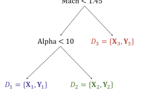
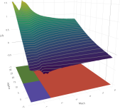
Figure 2: Left: Example of a tree generated by TGP on an LGBB dataset. Splits are made on speed (mach) and angle of attack (alpha). Right: Predictive surface plot of the rocket’s lift. The partition on the input space generated by the tree is shown on the bottom panel, with colors corresponding to respective leaf nodes.

A motivating example that showcases the benefits of the TGP model is the Langley Glide-Back Booster simulation (LGBB; Pamadi et al.,, 2004; Gramacy,, 2020, Chapter 2). The simulator emulates the dynamics of a rocket booster gliding through low Earth orbit. Inputs include the rocket’s speed (mach), angle of attack (alpha), and slip-side angle (beta); one of the outputs of interest is the resulting lift force. The dynamics of the simulator are known to drastically vary across mach values, specifically when speeds cross the sound barrier. TGP model-fitting entertains several different partitions of the three-dimensional input space. One of the more commonly generated trees is shown in the left panel of Figure 2, which heirarchically splits based on mach values of 1.45 and alpha values of 10. The predictive surface fit using the TGP model, averaging over all high-probability trees, is visualized in the surface plot on the right, where testing locations are fixed at a beta value of 1. The partition produced by the tree is illustrated underneath, on the $x$-$y$ plane; each color-coded region corresponds to one of the three leaf nodes contained in the tree on the left. The model appropriately partitions the input space where the dynamics of the response surface shift. It first chooses a split at the “divot” observed at speeds under 1.45, then decides to further divide that region based on smaller attack angles. Bitzer et al., (2023) recently expanded upon the TGP model by allowing for partitions based on hyperplanes which need not be axis-aligned (consider, for example, parallelograms instead of rectangles in the bottom plane of the right panel).

So far, the traditional divide-and-conquer GPs that we’ve discussed have focused on training data, via their inputs, as the “work” that is to be divided. What if we instead focused on the predictive locations as the avenue of division? After all, the over-arching objective of the surrogate model is to provide predictions (and UQ) at un-tried input configurations $X_{p}$. We can divide this “work” into $n_{p}$ jobs: predicting at each $\mathbf{x}_{k}\in X_{p}$ for $k=1,\dots,n_{p}$. Perhaps the earliest inspiration of this approach stems from “moving window” kriging methods in which kernel hyperparameters were estimated separately for each observation based on a local neighborhood (Haas,, 1990), generalizing the so-called “ordinary kriging” approach to geo-spatial modeling (Matheron,, 1971). Treating predictions as independent tasks sacrifices the ability to estimate the entire predictive covariance, $\bm{\Sigma}^{\star}$ in Eq. (2), but point-wise variance estimates are sufficient for most downstream surrogate modeling tasks.

Local approximate GPs (laGP; Gramacy and Apley,, 2015) combine independent GP predictions with strategic selection of conditioning sets. Rather than conditioning on the entire training data $\{X_{n},\mathbf{y}_{n}\}$ in Eq. (2), predictions for each $\mathbf{x}_{k}\in X_{p}$ condition on a strategically chosen subset $\{X_{n_{k}},\mathbf{y}_{n_{k}}\}$. Non-stationary flexibility comes from the independent nature of each GP; each $\mathbf{x}_{k}$ may have its own kernel hyperparameterization, thus allowing for the modeling of different dynamics at different locations. The original motivation for this work was to circumvent the cubic computational bottlenecks of GP inference that accompany large $n$ (by setting a maximum conditioning set size $|n_{k}|$), but the non-stationary flexibility has been a welcome byproduct (Sun et al.,, 2019). Just as partition GPs rely on a choice of partitioning scheme, local GPs rely on the choice of conditioning sets (Emery,, 2009). The rudimentary approach is to select the training data observations that are closest to $\mathbf{x}_{k}$ in Euclidean distance to populate $X_{n_{k}}$ – these are termed the “nearest neighbors”. In their seminal work, Gramacy and Apley, proposed strategic sequential selection of points in each conditioning set based on variance reduction criteria. The R package laGP offers a convenient wrapper for these local approximations (Gramacy,, 2016).

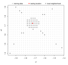
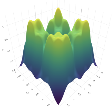
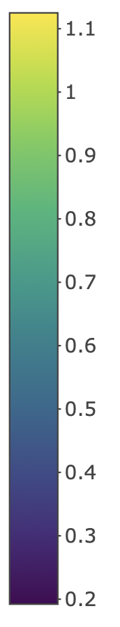
Figure 3: Left: Example of a local neighborhood (open circles), selected from a large training set (grey dots) for predicting at the red dot. Right: A global fit based on a patchwork laGPs applied over a dense testing set.

By dividing one big problem into many small ones, laGP avoids the cubic computational bottlenecks implicit in GP regression and creates an embarassingly parallel computational situation that is amenable to multi-core and distributed computing (Gramacy et al.,, 2014). The left panel of Figure 3 shows an example local neighborhood of size $n=50$ for predicting at the red dot. Each of the grey dots is one of $N>40K$ training data locations in $[-2,2]^{2}$. It goes without saying that you couldn’t fit an ordinary GP on a training data set that large, but you can use a local approximation over a vast testing grid to estimate a complex, non-stationary surface, as shown in the right panel of the figure. On an eight-core machine, the fit and prediction steps take less than minute.

Divide-and-conquer GPs bring non-stationary flexibility without any fancy machinery by relying on partitioned or local application of typical stationary GPs. Yet this flexibility comes at the expense of globality. The independent nature of the component GPs tosses out the ability to learn any global trends. As one such example, turn back to the Higdon function of Figure 1. [We omitted laGP from this exercise since local GPs are focused on large data sizes.] We presumed the training data was observed with an unknown noise variance, but assumed that the variance was constant across the entire space (aside from the hetGP model which was just for demonstration). It would be beneficial for a surrogate model to leverage all of the training data simultaneously, learning from the linear region that the data is noise-free and using that information to inform the interpolation of points in the left “wiggly” region. Yet divide-and-conquer GPs are instead tasked with estimating the noise independently on each division. The TGP fit in the lower left panel provides a clear visual; it created a partition in the middle of the space, fit separate GPs to both sides, but was unable to leverage information between the two sides. The search for a GP adaptation that is both global and non-stationary leads us to our final class of models – those that utilize spatial warpings.

5 Spatial warpings

Rather than adjusting the kernel or applying a multitude of independent GPs, “warped” GPs attempt to apply a regular stationary GP to a new input altogether. If the response is non-stationary over $X$-space, perhaps we can find a new space (let’s call it $W$-space) over which the response is plausibly stationary. Then a traditional GP prior from $W$ to $\mathbf{y}$, i.e., $\mathbf{y}\sim N\left(\bm{\mu},\bm{\Sigma}(W)\right)$ with stationary $\bm{\Sigma}(\cdot)$, would be an appropriate fit. We consider $W$ as a “warped” version of $X$, hence the name of this section; it is the driver of non-stationary flexibility. The characteristics of $W$ are a crucial modeling choice. Ideally the warping should be learned from training data (extensions that incorporate expert domain specific information are of interest, but not yet thoroughly explored), but finding an optimal and/or effective warping is a tall order.

Perhaps the earliest attempt to apply GPs on reformed inputs was from Sampson and Guttorp, (1992), who utilized “spatial dispersion” of the response values as the warping component. They expressed spatial covariance over the spatial dispersions rather than relative input distances, i.e., $\bm{\Sigma}_{\mathrm{ns}}(\mathbf{x}_{i},\mathbf{x}_{j})=\text{Cov}(y_{i}-y_{j})$. Spatial dispersions ($W$ in our notation) were learned through a combination of multi-dimensional scaling and spline interpolation, allowing for nonlinear warpings but not accounting for uncertainty in the learned warpings. Schmidt and O’Hagan, (2003) expanded upon this work by placing a GP prior over the warping, effectively creating the hierarchical model

$$\mathbf{y}_{n}\mid W \sim N\left(\bm{\mu}_{w},\bm{\Sigma}_{w}(W)\right)$$ (3)

$$W \sim N\left(\bm{\mu}_{x},\bm{\Sigma}_{x}(X_{n})\right).$$

This GP prior allowed for flexible nonlinear warpings and provided a natural avenue for uncertainty quantification surrounding $W$. They utilized Metropolis Hastings (MH) sampling of the unknown/latent $W$, wrapped in a Gibbs framework with various kernel hyperparameters. Schmidt and O’Hagan, thus created the first deep Gaussian process, although they did not name it as such. DGPs did not gain popularity until 10 years later when those in the ML community caught on to the idea and coined the DGP name (Damianou and Lawrence,, 2013), by analogy to DNNs – more on this parallel momentarily. There are several ways to compose a DGP, but the simplest is to link multiple GPs through functional compositions (3). This composition may be repeated to form deeper models. Intermediate layers remain unobserved/latent and must be inferred. Dunlop et al., (2018) have shown that this same model may be formulated through kernel convolutions, and is thus a special subset of the non-stationary kernel methods we discussed in Section 3.

There are several key distinctions between the original work of Schmidt and O’Hagan, and the DGPs that ML embraced a decade later. First, Schmidt and O’Hagan, focused on two-dimensional inputs, meaning their warping $W$ was a matrix of dimension $n\times 2$. They utilized a matrix Normal distribution over $W$ (our representation in Eq. (3) was strategically simplified), and in this smaller setting they were able to sample from the posterior distribution of the entire $W$ matrix using MH based schemes. This proved too much of a computational burden for expanding to higher dimensions. Damianou and Lawrence, (2013) proposed the simplication that each column of $W$ be conditionally independent, leaving the two-layer DGP prior as

$$\begin{aligned} \mathbf{y}_{n}\mid W&\sim N\left(\bm{\mu}_{w},\bm{\Sigma}_{w}(W)\right)\\ \mathbf{w}_{i}&\stackrel{{\scriptstyle\mathrm{ind}}}{{\sim}}N\left(\bm{\mu}_{x},\bm{\Sigma}_{x}(X_{n})\right),\;\;i=1,\dots,p\end{aligned}\quad\textrm{where}\quad W=\begin{bmatrix}\mathbf{w}_{1}&\mathbf{w}_{2}&\dots&\mathbf{w}_{p}\end{bmatrix}.$$

These columns are often referred to as “nodes”. The number of nodes is flexible, but most commonly set to match the input dimension, i.e., $p=d$. Now the parallel between DGPs and DNNs is clearer: a DGP is simply a DNN where the “activation functions” are Gaussian processes. Posterior inference requires integrating out the unknown latent warping,

$$\mathcal{L}(\mathbf{y}\mid X)=\int\dots\int\mathcal{L}(\mathbf{y}\mid W)\prod_{i=1}^{p}\mathcal{L}(\mathbf{w}_{i}\mid X)\;\;d\mathbf{w}_{1},\dots,d\mathbf{w}_{p},$$ (4)

which is not tractible in general. Extensions to deeper models require additional compositions of GPs, with even more unknown functional quantities to integrate (see Sauer et al.,, 2023, for thorough treatment of a three-layer DGP). Faced with this integral, many in ML embrace approximate variational inference (VI) in which the posterior of Eq. (4) is equated to the most likely distribution from a known target family (e.g., Damianou and Lawrence,, 2013; Bui et al.,, 2016; Salimbeni and Deisenroth,, 2017). This approach replaces integration with optimization, but in so doing it oversimplifies UQ. Additionally, it is unable to address the multi-modal nature of the posterior that is common in DGPs (Havasi et al.,, 2018).

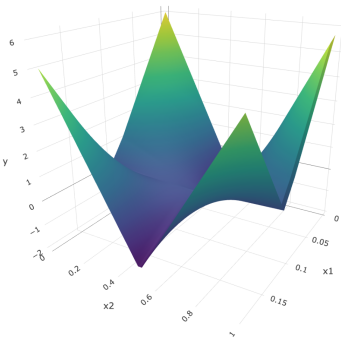
Figure 4: Left: The two-dimensional G-function. Right: A posterior ESS sample of latent layer $W$ from a two-layer DGP fit to training data from the G-function. Together, “nodes” of $W$ act as a warped verson of $X$, allowing the DGP to accommodate the steep inclines along the diagonals.

Surrogate modeling tasks demand broader uncertainty quantification. Full posterior integration through MCMC sampling of the latent warping offers the solution, but Metropolis Hastings type samplers have been shown to suffer from sticky chains and poor mixing in large DGP setups. To combat this, Sauer et al., (2023) proposed a fully-Bayesian inferential scheme for DGPs that employs elliptical slice sampling (ESS; Murray et al.,, 2010) of latent Gaussian layers. The rejection-free proposals of the ESS algorithm work well in DGP settings and are able to explore multiple modes more readily than MH counterparts. Others have embraced Hamiltonian Monte Carlo sampling as an alternative to ESS with similar outcomes (Havasi et al.,, 2018). Full propogation of uncertainty through posterior samples of $W$ is crucial for downstream surrogate modeling tasks including active learning (Sauer et al.,, 2023) and Bayesian optimization (Gramacy et al.,, 2022).

The fully-Bayesian MCMC implementation of DGPs is wrapped in the deepgp R-package on CRAN (Sauer,, 2022). We provide two visuals of DGP warping/flexibility utilizing this package. The first is shown in the lower center/right panels of Figure 1. The grey lines display ESS samples of latent $W$, fit to the training data from the Higdon function. The steep slope in the left region has the effect of “stretching” the inputs where there is high signal. The flattening-off of the samples in the right region effectively “squishes” inputs in the linear region. Notice how ESS samples of $W$ bounce back-and-forth between modes (positive slopes and negative slopes); since only pair-wise distances feature in the stationary kernel of the outer layer, these mirror images are equivalent. The resulting DGP fit is shown in the lower center panel; the warped model is able to accommodate the two piecewise regimes while leveraging global learning of kernel hyperparameters. The second visual concerns the two-dimensional G-function (Marrel et al.,, 2009), displayed in the left panel of Figure 4. This function is characterized by stiff peaks and steep valleys. In two dimensions, latent $W$ is comprised of two nodes, each a conditionally independent GP over the inputs. The right panel of Figure 4 visualizes a single ESS sample of $W$, interpreted as a warping from evenly gridded $X$. The response surface is plausibly stationary over this warped regime, thus allowing for superior non-stationary fits.

DGPs offer both global modeling and non-stationary flexibility, but they come with a hefty computational price tag. Posterior sampling requires thousands of samples, usually wrapped in a Gibbs scheme with many Gaussian likelihood evaluations required for each iteration. For training data sizes above several hundred, these computations become prohibitive. The machine learning approach – approximate inference by VI –partially addresses this issue by forcing DGPs into a neural network-style optimization problem, but it goes without saying that turning integration into optimization can severely undercut UQ. Moreover, this optimization of the Kullback-Leibler divergence between the desired DGP posterior and the specified target family requires thousands of iterations, on par with the iterations needed for MCMC mixing. Consequently, the speedups offered by VI are marginal at best. Big computational gains require further approximation. The predominant tool here is inducing points (IPs; Snelson and Ghahramani,, 2006); all of the VI references we have mentioned so far, as well as the Hamiltonian Monte Carlo sampling implementation of Havasi et al., (2018), make use of IP approximations. But IPs come with several pitfalls: without large quantities and/or optimal placement, they provide blurry low-fidelity predictions (Wu et al.,, 2022). Some have embraced random feature expansions as alternatives to inducing points (Marmin and Filippone,, 2022), but perhaps the most successful alternative has been Vecchia approximation (Vecchia,, 1988; Sauer et al.,, 2022). The Vecchia approximation forms the basis of scalability in the deepGP package. In our own experience, the Vecchia-based DGP approach is more robust and user friendly – offering more accurate predictions with better UQ out of the box – compared to VI/IP alternatives, and others in similar spirit such as the Python libraries GPflux (Dutordoir et al.,, 2021) and GPyTorch (Gardner et al.,, 2018). Occasionally we can fine-tune these libraries to get competitive results in terms of accuracy, but UQ still suffers distinctly.

6 A final experiment

As a concluding demonstration, we present a comparison of the aforementioned non-stationary GP surrogates on a real-world computer simulation. The Test Particle Monte Carlo simulator was developed by researchers at Los Alamos National Laboratory to simulate the movement of satellites in low earth orbit (Mehta et al.,, 2014). The simulation is contingent on the specification of a satellite mesh. Sauer et al., (2022) entertained non-stationary DGP surrogates on the GRACE satellite; we instead consider the Hubble space telescope, which has an additional input parameter, bumping the problem up to 8-dimensions. The response variable is the amount of atmostpheric drag experienced by the satellite. See Gramacy, (2020, Chapter 2) for further narration of this simulation suite.

We utilize a data set of 1 million simulation runs provided by Sun et al., (2019), selecting disjoint random subsets of size $n=n_{p}=10{,}000$ for training and testing. We entertain the following surrogate models:

• GP SVEC: stationary GP utilizing scaled-Vecchia approximation (Katzfuss et al.,, 2020).

• laGP: local approximate GP (Gramacy and Apley,, 2015) using the laGP package (Gramacy,, 2016).

• TGP: treed-GP (Gramacy and Lee,, 2008) using the tgp package (Gramacy,, 2007).

• DGP ESS: Bayesian DGP with elliptical slice sampling and Vecchia approximation (Sauer et al.,, 2023, 2022) using the deepgp package (Sauer,, 2022).

• DGP DSVI: DGP with approximate “doubly stochastic” variational inference and inducing point approximations (Salimbeni and Deisenroth,, 2017) using the GPflux package (Dutordoir et al.,, 2021).

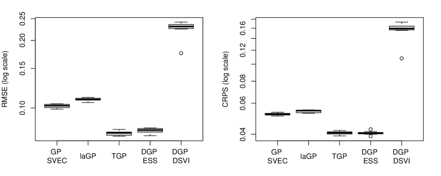
Figure 5: Surrogate performance on the 8-dimensional Hubble Space Telescope simulation across 10 MC repetitions.

We follow Sun et al., (2019) in fixing the noise level at $\nu=1\times 10^{-4}$. Separable lengthscales estimated from the GP SVEC model are used to pre-scale inputs prior to fitting the other surrogate models [except for TGP since the tgp package conducts its own scaling]. Input pre-scaling and similar analogues have been shown to improve surrogate performance and have become standard (e.g., Sun et al.,, 2019; Katzfuss et al.,, 2020; Wycoff et al.,, 2021; Kang and Katzfuss,, 2023). Model performance is reported by root mean squared error (RMSE, lower is better) and continuous rank probability score (CRPS; Gneiting and Raftery,, 2007, Eq. 20, negated so lower is better). While RMSE captures surrogate predictive accuracy, CRPS incorporates posterior UQ. Results across 10 Monte Carlo repetitions, with re-randomized training and testing sets, are shown in Figure 5. Reproducible code for this experiment is provided in our public git repository.

Of the five methods, DSVI’s approach to deep GP inference stands out as being particularly poor. We don’t have a good explanation for that except that the class of problems it was engineered for – low-signal large-data regression and classification for machine learning tasks – is different than our computer modeling context, with modest training data size and high signal-to-noise ratios. We know VI undercuts on UQ, and we suspect the IPs sacrifice too much fidelity in this instance. Observe that laGP performs relatively well, but interestingly not as well as an ordinary GP (represented by GP SVEC). Our explanation here is that laGP was designed for massive data settings on the scale of millions of observations. It was developed primarily with speed and parallelization in mind, with non-stationary flexibility being a byproduct of its divide-and-conquer approach. These data do indeed benefit from deliberate non-stationary modeling, as indicated by the TGP and DGP ESS comparators. We believe TGP edges out DGP on this example because the process benefits from crude, axis-aligned partitioning. We observed a high degree of TGP partitioning on the eighth, “panel-angle” input. It would seem the orientation of Hubble’s solar panels is driving regime changes in drag dynamics. Both TGP and DGP ESS utilize a fully Bayesian approach to inference for all unknown quantities. Consequently they have high predictive accuracy (via RMSE) and UQ (via CRPS).

References

- Andrianakis et al., (2015) Andrianakis, I., Vernon, I. R., McCreesh, N., McKinley, T. J., Oakley, J. E., Nsubuga, R. N., Goldstein, M., and White, R. G. (2015). “Bayesian history matching of complex infectious disease models using emulation: a tutorial and a case study on HIV in Uganda.” PLoS computational biology, 11, 1, e1003968.
- Baker et al., (2022) Baker, E., Barbillon, P., Fadikar, A., Gramacy, R. B., Herbei, R., Higdon, D., Huang, J., Johnson, L. R., Ma, P., Mondal, A., et al. (2022). “Analyzing stochastic computer models: A review with opportunities.” Statistical Science, 37, 1, 64–89.
- Banerjee et al., (2003) Banerjee, S., Carlin, B. P., and Gelfand, A. E. (2003). Hierarchical modeling and analysis for spatial data. Chapman and Hall/CRC.
- Binois and Gramacy, (2021) Binois, M. and Gramacy, R. B. (2021). “hetGP: Heteroskedastic Gaussian Process Modeling and Sequential Design in R.” Journal of Statistical Software, 98, 13, 1–44.
- Binois et al., (2018) Binois, M., Gramacy, R. B., and Ludkovski, M. (2018). “Practical heteroscedastic gaussian process modeling for large simulation experiments.” Journal of Computational and Graphical Statistics, 27, 4, 808–821.
- Binois et al., (2019) Binois, M., Huang, J., Gramacy, R. B., and Ludkovski, M. (2019). “Replication or exploration? Sequential design for stochastic simulation experiments.” Technometrics, 61, 1, 7–23.
- Binois and Wycoff, (2022) Binois, M. and Wycoff, N. (2022). “A survey on high-dimensional Gaussian process modeling with application to Bayesian optimization.” ACM Transactions on Evolutionary Learning and Optimization, 2, 2, 1–26.
- Bitzer et al., (2023) Bitzer, M., Meister, M., and Zimmer, C. (2023). “Hierarchical-Hyperplane Kernels for Actively Learning Gaussian Process Models of Nonstationary Systems.” In International Conference on Artificial Intelligence and Statistics, 7897–7912. PMLR.
- Bornn et al., (2012) Bornn, L., Shaddick, G., and Zidek, J. V. (2012). “Modeling nonstationary processes through dimension expansion.” Journal of the American Statistical Association, 107, 497, 281–289.
- Bui et al., (2016) Bui, T., Hernández-Lobato, D., Hernandez-Lobato, J., Li, Y., and Turner, R. (2016). “Deep Gaussian processes for regression using approximate expectation propagation.” In International conference on machine learning, 1472–1481. PMLR.
- Chipman et al., (1998) Chipman, H. A., George, E. I., and McCulloch, R. E. (1998). “Bayesian CART model search.” Journal of the American Statistical Association, 93, 443, 935–948.
- Cressie, (2015) Cressie, N. (2015). Statistics for spatial data. John Wiley & Sons.
- Damianou and Lawrence, (2013) Damianou, A. and Lawrence, N. D. (2013). “Deep gaussian processes.” In Artificial intelligence and statistics, 207–215. PMLR.
- Dunlop et al., (2018) Dunlop, M. M., Girolami, M. A., Stuart, A. M., and Teckentrup, A. L. (2018). “How deep are deep Gaussian processes?” Journal of Machine Learning Research, 19, 54, 1–46.
- Dutordoir et al., (2021) Dutordoir, V., Salimbeni, H., Hambro, E., McLeod, J., Leibfried, F., Artemev, A., van der Wilk, M., Deisenroth, M. P., Hensman, J., and John, S. (2021). “GPflux: A library for Deep Gaussian Processes.” arXiv:2104.05674.
- Emery, (2009) Emery, X. (2009). “The kriging update equations and their application to the selection of neighboring data.” Computational Geosciences, 13, 3, 269–280.
- Eriksson et al., (2019) Eriksson, D., Pearce, M., Gardner, J., Turner, R. D., and Poloczek, M. (2019). “Scalable global optimization via local bayesian optimization.” Advances in neural information processing systems, 32.
- Gardner et al., (2018) Gardner, J., Pleiss, G., Weinberger, K. Q., Bindel, D., and Wilson, A. G. (2018). “Gpytorch: Blackbox matrix-matrix gaussian process inference with gpu acceleration.” Advances in neural information processing systems, 31.
- Gneiting and Raftery, (2007) Gneiting, T. and Raftery, A. E. (2007). “Strictly proper scoring rules, prediction, and estimation.” Journal of the American statistical Association, 102, 477, 359–378.
- Gramacy et al., (2014) Gramacy, R., Niemi, J., and Weiss, R. (2014). “Massively parallel approximate Gaussian process regression.” SIAM/ASA Journal on Uncertainty Quantification, 2, 1, 564–584.
- Gramacy, (2007) Gramacy, R. B. (2007). “tgp: An R Package for Bayesian Nonstationary, Semiparametric Nonlinear Regression and Design by Treed Gaussian Process Models.” Journal of Statistical Software, 19, 9, 1–46.
- Gramacy, (2016) — (2016). “laGP: Large-Scale Spatial Modeling via Local Approximate Gaussian Processes in R.” Journal of Statistical Software, 72, 1, 1–46.
- Gramacy, (2020) — (2020). Surrogates: Gaussian Process Modeling, Design and Optimization for the Applied Sciences. Boca Raton, Florida: Chapman Hall/CRC. Http://bobby.gramacy.com/surrogates/.
- Gramacy and Apley, (2015) Gramacy, R. B. and Apley, D. W. (2015). “Local Gaussian process approximation for large computer experiments.” Journal of Computational and Graphical Statistics, 24, 2, 561–578.
- Gramacy et al., (2004) Gramacy, R. B., Lee, H. K., and Macready, W. G. (2004). “Parameter space exploration with Gaussian process trees.” In Proceedings of the twenty-first international conference on Machine learning, 45.
- Gramacy and Lee, (2008) Gramacy, R. B. and Lee, H. K. H. (2008). “Bayesian treed Gaussian process models with an application to computer modeling.” Journal of the American Statistical Association, 103, 483, 1119–1130.
- Gramacy et al., (2022) Gramacy, R. B., Sauer, A., and Wycoff, N. (2022). “Triangulation candidates for Bayesian optimization.” Advances in Neural Information Processing Systems, 35, 35933–35945.
- Graßhoff et al., (2020) Graßhoff, J., Jankowski, A., and Rostalski, P. (2020). “Scalable Gaussian process separation for kernels with a non-stationary phase.” In International Conference on Machine Learning, 3722–3731. PMLR.
- Haas, (1990) Haas, T. C. (1990). “Kriging and automated variogram modeling within a moving window.” Atmospheric Environment. Part A. General Topics, 24, 7, 1759–1769.
- Havasi et al., (2018) Havasi, M., Hernández-Lobato, J. M., and Murillo-Fuentes, J. J. (2018). “Inference in deep gaussian processes using stochastic gradient hamiltonian monte carlo.” In Advances in neural information processing systems, 7506–7516.
- Heinonen et al., (2016) Heinonen, M., Mannerström, H., Rousu, J., Kaski, S., and Lähdesmäki, H. (2016). “Non-stationary gaussian process regression with hamiltonian monte carlo.” In Artificial Intelligence and Statistics, 732–740. PMLR.
- Higdon et al., (1999) Higdon, D., Swall, J., and Kern, J. (1999). “Non-stationary spatial modeling.” Bayesian statistics, 6, 1, 761–768.
- Huang et al., (2021) Huang, H., Blake, L. R., Katzfuss, M., and Hammerling, D. M. (2021). “Nonstationary Spatial Modeling of Massive Global Satellite Data.” arXiv preprint arXiv:2111.13428.
- Johnson, (2008) Johnson, L. (2008). “Microcolony and biofilm formation as a survival strategy for bacteria.” Journal of Theoretical Biology, 251, 24–34.
- Jones et al., (1998) Jones, D. R., Schonlau, M., and Welch, W. J. (1998). “Efficient global optimization of expensive black-box functions.” Journal of Global optimization, 13, 4, 455.
- Kang and Katzfuss, (2023) Kang, M. and Katzfuss, M. (2023). “Correlation-based sparse inverse Cholesky factorization for fast Gaussian-process inference.” Statistics and Computing, 33, 3, 56.
- Katzfuss, (2013) Katzfuss, M. (2013). “Bayesian nonstationary spatial modeling for very large datasets.” Environmetrics, 24, 3, 189–200.
- Katzfuss et al., (2020) Katzfuss, M., Guinness, J., and Lawrence, E. (2020). “Scaled Vecchia approximation for fast computer-model emulation.” arXiv preprint arXiv:2005.00386.
- Kennedy and O’Hagan, (2001) Kennedy, M. C. and O’Hagan, A. (2001). “Bayesian calibration of computer models.” Journal of the Royal Statistical Society: Series B (Statistical Methodology), 63, 3, 425–464.
- Kim et al., (2005) Kim, H.-M., Mallick, B. K., and Holmes, C. C. (2005). “Analyzing nonstationary spatial data using piecewise Gaussian processes.” Journal of the American Statistical Association, 100, 470, 653–668.
- Koermer et al., (2023) Koermer, S., Loda, J., Noble, A., and Gramacy, R. B. (2023). “Active Learning for Simulator Calibration.” arXiv preprint arXiv:2301.10228.
- Marmin and Filippone, (2022) Marmin, S. and Filippone, M. (2022). “Deep Gaussian Processes for Calibration of Computer Models.” Bayesian Analysis, 1 – 30.
- Marrel et al., (2009) Marrel, A., Iooss, B., Laurent, B., and Roustant, O. (2009). “Calculations of Sobol indices for the Gaussian process metamodel.” Reliability Engineering & System Safety, 94, 3, 742–751.
- Marten et al., (2013) Marten, D., Wendler, J., Pechlivanoglou, G., Nayeri, C. N., and Paschereit, C. O. (2013). “QBLADE: an open source tool for design and simulation of horizontal and vertical axis wind turbines.” International Journal of Emerging Technology and Advanced Engineering, 3, 3, 264–269.
- Matheron, (1971) Matheron, G. (1971). The Theory of Regionalized Variables and Its Applications. Fontaineblue, Paris: Les Cahiers du Centre de Morphologie Mathematique.
- Mehta et al., (2014) Mehta, P., Walker, A., Lawrence, E., Linares, R., Higdon, D., and Koller, J. (2014). “Modeling satellite drag coefficients with response surfaces.” Advances in Space Research, 54, 8, 1590–1607.
- Moran et al., (2022) Moran, K. R., Heitmann, K., Lawrence, E., Habib, S., Bingham, D., Upadhye, A., Kwan, J., Higdon, D., and Payne, R. (2022). “The Mira-Titan Universe–IV. High precision power spectrum emulation.” Monthly Notices of the Royal Astronomical Society.
- Murray et al., (2010) Murray, I., Adams, R. P., and MacKay, D. J. C. (2010). “Elliptical slice sampling.” In The Proceedings of the 13th International Conference on Artificial Intelligence and Statistics, vol. 9 of JMLR: W&CP, 541–548. PMLR.
- Noack et al., (2023) Noack, M. M., Krishnan, H., Risser, M. D., and Reyes, K. G. (2023). “Exact Gaussian processes for massive datasets via non-stationary sparsity-discovering kernels.” Scientific reports, 13, 1, 3155.
- Nychka et al., (2018) Nychka, D., Hammerling, D., Krock, M., and Wiens, A. (2018). “Modeling and emulation of nonstationary Gaussian fields.” Spatial statistics, 28, 21–38.
- Nychka et al., (2002) Nychka, D., Wikle, C., and Royle, J. A. (2002). “Multiresolution models for nonstationary spatial covariance functions.” Statistical Modelling, 2, 4, 315–331.
- Paciorek and Schervish, (2003) Paciorek, C. J. and Schervish, M. J. (2003). “Nonstationary Covariance Functions for Gaussian Process Regression.” In Proceedings of the 16th International Conference on Neural Information Processing Systems, NIPS’03, 273–280. Cambridge, MA, USA: MIT Press.
- Pamadi et al., (2004) Pamadi, B., Covell, P., Tartabini, P., and Murphy, K. (2004). “Aerodynamic characteristics and glide-back performance of langley glide-back booster.” In 22nd Applied Aerodynamics Conference and Exhibit, 5382.
- Plumlee et al., (2016) Plumlee, M., Joseph, V. R., and Yang, H. (2016). “Calibrating functional parameters in the ion channel models of cardiac cells.” Journal of the American Statistical Association, 111, 514, 500–509.
- Rasmussen and Ghahramani, (2001) Rasmussen, C. and Ghahramani, Z. (2001). “Infinite mixtures of Gaussian process experts.” Advances in neural information processing systems, 14.
- Rasmussen and Williams, (2005) Rasmussen, C. E. and Williams, C. K. I. (2005). Gaussian Processes for Machine Learning. Cambridge, Mass.: MIT Press.
- Renganathan et al., (2021) Renganathan, S. A., Maulik, R., and Ahuja, J. (2021). “Enhanced data efficiency using deep neural networks and Gaussian processes for aerodynamic design optimization.” Aerospace Science and Technology, 111, 106522.
- Risser and Calder, (2017) Risser, M. D. and Calder, C. A. (2017). “Local Likelihood Estimation for Covariance Functions with Spatially-Varying Parameters: The convoSPAT Package for R.” Journal of Statistical Software, 81, 14, 1–32.
- Salimbeni and Deisenroth, (2017) Salimbeni, H. and Deisenroth, M. (2017). “Doubly stochastic variational inference for deep Gaussian processes.” arXiv preprint arXiv:1705.08933.
- Sampson and Guttorp, (1992) Sampson, P. D. and Guttorp, P. (1992). “Nonparametric estimation of nonstationary spatial covariance structure.” Journal of the American Statistical Association, 87, 417, 108–119.
- Santner et al., (2018) Santner, T., Williams, B., and Notz, W. (2018). The Design and Analysis of Computer Experiments, Second Edition. New York, NY: Springer–Verlag.
- Sauer, (2022) Sauer, A. (2022). deepgp: Deep Gaussian Processes using MCMC. R package version 1.1.0.
- Sauer et al., (2022) Sauer, A., Cooper, A., and Gramacy, R. B. (2022). “Vecchia-approximated deep Gaussian processes for computer experiments.” Journal of Computational and Graphical Statistics, 1–14.
- Sauer et al., (2023) Sauer, A., Gramacy, R. B., and Higdon, D. (2023). “Active learning for deep Gaussian process surrogates.” Technometrics, 65, 1, 4–18.
- Schmidt and O’Hagan, (2003) Schmidt, A. M. and O’Hagan, A. (2003). “Bayesian inference for non-stationary spatial covariance structure via spatial deformations.” Journal of the Royal Statistical Society: Series B (Statistical Methodology), 65, 3, 743–758.
- Snelson and Ghahramani, (2006) Snelson, E. and Ghahramani, Z. (2006). “Sparse Gaussian Processes using Pseudo-inputs.” Advances in Neural Information Processing Systems 18, 1257–1264.
- Stanford et al., (2022) Stanford, B., Sauer, A., Jacobson, K., and Warner, J. (2022). “Gradient-Enhanced Reliability Analysis of Transonic Aeroelastic Flutter.” In AIAA SCITECH 2022 Forum, 0632.
- Stein, (1999) Stein, M. L. (1999). Interpolation of spatial data: some theory for kriging. Springer Science & Business Media.
- Sun et al., (2019) Sun, F., Gramacy, R. B., Haaland, B., Lawrence, E., and Walker, A. (2019). “Emulating satellite drag from large simulation experiments.” SIAM/ASA Journal on Uncertainty Quantification, 7, 2, 720–759.
- Turek and Risser, (2022) Turek, D. and Risser, M. (2022). BayesNSGP: Bayesian Analysis of Non-Stationary Gaussian Process Models. R package version 0.1.2.
- Vecchia, (1988) Vecchia, A. V. (1988). “Estimation and model identification for continuous spatial processes.” Journal of the Royal Statistical Society: Series B (Methodological), 50, 2, 297–312.
- Wang et al., (2020) Wang, K., Hamelijnck, O., Damoulas, T., and Steel, M. (2020). “Non-separable Non-stationary random fields.” In International Conference on Machine Learning, 9887–9897. PMLR.
- Wu et al., (2022) Wu, L., Pleiss, G., and Cunningham, J. (2022). “Variational Nearest Neighbor Gaussian Processes.” arXiv preprint arXiv:2202.01694.
- Wycoff et al., (2021) Wycoff, N., Binois, M., and Gramacy, R. B. (2021). “Sensitivity prewarping for local surrogate modeling.” arXiv preprint arXiv:2101.06296.