Learning for Robust Optimization

Abstract

We propose a data-driven technique to automatically learn the uncertainty sets in robust optimization. Our method reshapes the uncertainty sets by minimizing the expected performance across a family of problems while guaranteeing constraint satisfaction. We learn the uncertainty sets using a novel stochastic augmented Lagrangian method that relies on differentiating the solutions of the robust optimization problems with respect to the parameters of the uncertainty set. We show sublinear convergence to stationary points under mild assumptions, and finite-sample probabilistic guarantees of constraint satisfaction using empirical process theory. Our approach is very flexible and can learn a wide variety of uncertainty sets while preserving tractability. Numerical experiments show that our method outperforms traditional approaches in robust and distributionally robust optimization in terms of out of sample performance and constraint satisfaction guarantees. We implemented our method in the open-source package LROPT.

1 Introduction

Over the past years, robust optimization (RO) has become a widely adopted efficient tool for decision-making under uncertainty. The idea behind RO is to define an uncertainty set where the uncertainty lives and, then, optimize against the worst-case realizations of the uncertainty in this set; see [BTEGN09, BdH22] and survey papers [BTN08, BBC11] for a thorough review. The choice of the uncertainty sets is a crucial component of RO, and can have a significant impact on the solution quality and robustness. While well-chosen uncertainty sets can lead to optimal solutions with high performance and robustness, poorly chosen sets may result in solutions that are overly conservative or that have low probability of constraint satisfaction. For this reason, a large amount of existing literature studies how to bound the probability of constraint satisfaction based on the size and shape of the uncertainty sets [LTF12, GMF17, BdP19]. In this vein, many approaches to designing uncertainty sets assume structural information of the unknown distributions, and rely on these a priori assumptions to build guarantees of constraint satisfaction [BTN00, BB12, BTEGN09, BS04]. However, these assumptions may be unrealistic or difficult to verify in practice, and the resulting theoretical guarantees may be too conservative experimentally [RdH20, GK16].

In contrast, the recent explosion in the availability of data has lead to new paradigms where uncertainty sets are designed directly from data [BGK18]. By combining a priori assumptions with the confidence regions of statistical hypothesis tests on the data [BGK18], or by approximating a high-probability-region using quantile estimation [HHL21], recent techniques construct data-driven uncertainty sets that yield less conservative solutions while retaining robustness. However, these methods still rely on strong a-priori assumptions on the probability distribution of the uncertainty, such as finite support or independent marginals. In addition, the majority of the RO literature relies on building uncertainty sets that contain the vast majority of the probability mass. However, that’s only a sufficient (and often restrictive) condition to guarantee high probability of constraint satisfaction [BTEGN09, page 33]. While Bertsimas et al. [BGK18] avoid such restrictions by exploiting the dependence of the uncertain constraint on uncertain parameter set, their technique can only deal with joint chance constraints via union-bounds, which can be conservative. Instead, we turn our attention to RO techniques that can directly tackle joint chance constraints using direct hyperparameter tuning.

While cross-validation has been long-standing in machine learning and related fields for hyperparameter selection [Koh01], recently, implicit differentiation techniques have led to the possibility of tuning high-dimensional hyperparameters through gradient-based approaches, which are much more efficient than grid search or manual tuning [BKM⁺]. However, the RO community has seen limited efforts in automating the choice of the uncertainty sets [BGK18, HHL21] most of which do not exploit recent hyperparameter tuning approaches. That’s why, most techniques manually calibrate the uncertainty sets using grid-search and cross-validation by varying a single parameter, often the size of the uncertainty set. In this work, we propose a technique to learn multiple parameters of the uncertainty sets at the same time, including shape and size.

Finally, most RO formulations suffer from the fact that we calibrate uncertainty sets for a specific problem instance, while we often solve a family of similar optimization problems with varying parameters. This is a common scenario in many applications, including inventory management, where we solve similar optimization problems with varying initial inventory levels while satisfying uncertain demand with high probability.

In this work, we propose an automatic technique to learn the RO uncertainty sets from data. Our method minimizes an expected objective over a family of parametrized problems, while ensuring data-driven constraint satisfaction guarantees. We tune the uncertainty sets with a stochastic augmented Lagrangian approach relying on implicit differentiation techniques [ABB⁺19, AAB⁺19] to compute the derivative of the solution of robust optimization problems with respect to key parameters of the uncertainty sets. By incorporating the problem objective and the data-driven constraint satisfaction into the learning problem, we control the tradeoff between performance and robustness. Lastly, to show finite sample probabilistic guarantees of constraint satisfaction, we use empirical process theory and a covering number argument, which have been common in distributionally robust optimization (DRO) literature [ILW22, ND17, SNVD20, GCK0].

1.1 Our contributions

In this work, we present a new approach to automatically learn the uncertainty sets in RO to obtain high-quality solutions across a family of problems while ensuring probabilistic guarantees of constraint satisfaction.

• We formulate the problem of finding the uncertainty set using bi-level optimization. At the outer level, we minimize the expectation of the objective function over the family of parametric optimization problems, while ensuring an appropriate probability level of constraint satisfaction. At the lower level, we represent the decisions as the solution of the resulting RO problem.

• To solve the above problem and find the optimal parameters of the uncertainty set, we develop a stochastic augmented Lagrangian approach. We also show its convergence and finite sample probabilistic guarantees of constraint satisfaction.

• We implement our technique in Python package learning for robust optimization (LROPT), which allows users to easily model and tune uncertainty sets in RO. The code is available at https://github.com/stellatogrp/lropt.

• We benchmark our method on various examples in portfolio optimizatio, multi-product newsvendor, and multi-stage inventory management, outperforming data-driven robust and distributionally robust approaches in terms of out-of-sample objective value and probabilistic guarantees, and execution time after training.

1.2 Related work

Data-driven robust optimization.

With the recent explosion of availability of data, data-driven robust optimization, has gained wide popularity. These techniques often approximate the unknown data-generating distribution in order to construct data-driven uncertainty sets. Using hypothesis testing, Bertsimas et al. [BGK18] pair a priori assumptions on the distribution with different statistical tests, and obtain various uncertainty sets with different shapes, computational properties, and modeling power. Similar approaches construct data-driven sets using quantile estimation [HHL21] and deep learning clustering techniques [GK23]. All these approaches rely on a two-step procedure which separates the construction of the uncertainty set from the resulting robust optimization problem. Because of the possible suboptimality caused by this separation, Costa and Iyengar [CI22] propose an end-to-end distributionally robust approach in the context of portfolio construction, where the solution to the robust optimization problem and the selection of the ambiguity set are trained together in an end-to-end fashion. They integrate a prediction layer that predicts asset returns with data on financial features and historical returns, and use these predictions in a decision layer that incorporates the robust optimization problem. Our approach follows this idea of an end-to-end approach, but provides a more general framework for a larger class of robust optimization problems and is able to adjust the shape of the uncertainty sets.

Modeling languages for robust optimization

Several open-source packages facilitate building models for RO, including as ROME [GS09] in Matlab, RSOME [XC21] in Python, JuMPeR [Dun] in Julia, and ROmodel [WM21] for the Pyomo modeling language in Python. These packages mostly support RO problems with affine uncertain constraints, which are solved via reformulations and/or cutting plane procedures. Schiele et al.[SLB23] recently introduced a Python extension of CVXPY [DB16] for solving the larger class of convex-concave saddle point problems, by automating a conic dualization procedure reformulating min-max type problems into min-min problems which can then be solved efficiently [JN22]. In the paper, they describe a set of rules termed disciplined saddle programming (DSP) detailing when a saddle point optimization problem can be equivalently formulated as convex optimization ones, and efficiently be solved. In this work, we build a Python extension to CVXPY tailored to formulating and solving RO problems. While some RO problems can be described in terms of the DSP framework, our library augments DSP capabilities in RO by supporting max-of-concave uncertain constraint and structure to intuitively describe well known uncertainty sets for ease of use. Finally, with our method automatically learns of the uncertainty set through differentiable optimization via a tight integration with [AAB⁺19, ABB⁺19].

Differentiable convex optimization.

There has been extensive work on embedding differentiable optimization problems as layers within deep learning architectures [AK21]. The authors of [AAB⁺19] propose an approach to differentiating through disciplined convex programs and implement their methodology in CVXPY, and additionally implement differentiable layers for disciplined convex programs in PyTorch and TensorFlow 2.0, Cvxpylayers. These developments have enabled the popualar end-to-end approach of training a predictive model to minimize loss on a downstream optimization task [EG22, CHLLB21, DAK17, DSB⁺19, WDT19, WEDT19], for which we also point to the survey [KFVHW21]. These approaches with the Smart Predict, then Optimize framework [EG22] have been shown to improve performace as opposed to traditional two-stage approaches, where the model is trained separately from the optimization problem [CI22]. Our approach thus adopts the idea of end-to-end learning by linking the process of constructing the uncertainty set to the inner robust optimization problem.

Automatic hyperparameter selection.

Implicit differentiation techniques can greatly accelerate tuning the regularization parameters in regression and classification problems [BKB⁺20, BKM⁺, BKMZ19]. However, most literature focuses on tuning hyperparameters of the objective function in regression and classification tasks, such as hyper-parameters for Lasso regularization [BKM⁺]. In this work, we tune various hyperparameters of the uncertainty sets in RO using implicit differentiation techniques.

1.3 Layout of the paper

In Section 2, we introduce the notion of the reshaping parameters with a motivating example, and in Section 3, we describe the data-driven problem and the algorithm for learning reshaping parameters. In Section 4, we discuss the probabilistic guarantees implied by the aforementioned formulations. In Section 5, we give a high-level overview of our LROPT package, and in Section 6, we present various numerical examples problems. For completeness, we give example convex reformulations of robust optimization problems for common uncertainty sets in the appendices.

2 The robust optimization problem

We consider a family of robust optimization (RO) problems parametrized by a family parameter $y\in{\mbox{\bf R}}^{p}$ with distribution ${\mathbf{P}}_{y}$. Each problem has the form

$$x(\theta,y)\in\begin{array}[t]{ll}\mathop{\rm argmin}&f(x,y)\\ \mbox{subject to}&g(x,u,y)\leq 0\quad\forall u\in{\mathcal{U}}(\theta),\end{array}$$ (1)

where $x\in{\mbox{\bf R}}^{n}$ is the optimization variable, $u\in{\mbox{\bf R}}^{m}$ is the uncertain parameter, $f:{\mbox{\bf R}}^{n}\times{\mbox{\bf R}}^{p}\to{\mbox{\bf R}}$ is the objective function, and $g:{\mbox{\bf R}}^{n}\times{\mbox{\bf R}}^{m}\times{\mbox{\bf R}}^{p}\to{\mbox{\bf R}}^{d}$ is the uncertain constraint which we assume to be the maximum of concave functions, e.g., $g(x,u,y)=\max_{l=1,\dots,L}g_{l}(x,u,y)$. This structure allows us to express $L$ joint uncertain constraints using the maximum of each component $l$. The uncertain parameter $u$ takes values from ${\mathcal{U}}(\theta)\subseteq{\mbox{\bf R}}^{m}$, a convex uncertainty set parametrized by $\theta\in{\mbox{\bf R}}^{q}$. The family parameter $y$ differs from the uncertain parameter $u$ in that it is known when we make the decision. We refer to instances of the family as the realization of problem (1) where $y$ takes a specific value. Note that, if $y$ is supported on a single value, we obtain the usual RO formulation.

Our goal is to find a parameter $\theta$ such that the solutions $x(\theta,y)$ perform well in terms of objective value and constraint satisfaction guarantees across the family of problems. As learning an uncertainty set is costly, we don’t learn a separate uncertainty set for every instance of the family. Instead, we construct a set that works for all members of the family simultaneously. More formally, we choose the uncertainty set such that the solution $x(\theta,y)$ from (1) implies that the uncertain constraint is satisfied with high probability across instances of the problem family:

$${\mathbf{P}}_{(u,y)}(g(x(\theta,y),u,y)\leq 0)\geq 1-\eta,$$ (2)

for a given $\eta>0$, where ${\mathbf{P}}_{(u,y)}$ is the joint distribution of $u$ and $y$. We can formulate this constraint in terms of the corresponding value at risk being nonpositive, i.e.,

$$\mathop{\bf VaR}(g(x(\theta,y),u,y),\eta)=\inf\{\gamma\mid{\mathbf{P}}_{(u,y)}(g(x(\theta,y),u,y)\leq\gamma)\geq 1-\eta\}\leq 0.$$

Unfortunately, except in very special cases, the value at risk function is intractable [UR01]. To get a tractable approximation, we can adopt the conditional value at risk [UR01, RU02], defined as

$$\mathop{\bf CVaR}(g(x(\theta,y),u,y),\eta)=\inf_{\alpha}\{{\mbox{\bf E}}_{(u,y)}((1/\eta)(g(x(\theta,y),u,y)-\alpha)_{+})+\alpha\},$$ (3)

where $(a)_{+}=\max\{a,0\}$. It is well known from [UR01] that, for any $x\in{\mbox{\bf R}}^{n}$, the relationship between these probabilistic guarantees of constraint satisfaction is

$$\mathop{\bf CVaR}(g(x,u,y),\eta)\leq 0~{}~{}\Longrightarrow~{}~{}\mathop{\bf VaR}(g(x,u,y),\eta)\leq 0~{}~{}\Longleftrightarrow~{}~{}{\mathbf{P}}(g(x,u,y)\leq 0)\geq 1-\eta.$$ (4)

Therefore, if the solution $x(\theta,y)$ of (1) satisfies $\mathop{\bf CVaR}(g(x(\theta,y),u,y),\eta)\leq 0$, we have the desired probabilistic guarantee (2).

By constructing uncertainty sets that contain at least $1-\eta$ probability mass, i.e., ${\mathbf{P}}(u\in{\mathcal{U}}(\theta))\geq 1-\eta$, we can ensure that any feasible solution of (1) implies a probabilistic guarantee (2). However, this condition is only sufficient, and may lead to overly conservative solutions [BTEGN09, page 33]. In this work, instead, we avoid such conservatism by taking into account the cost of the robust solutions $x(\theta,y)$ while constructing the uncertainty sets.

2.1 Motivating example

We consider a newsvendor problem where, at the beginning of each day, the vendor orders $x\in{\mbox{\bf R}}^{n}$ products at price $k\in{\mbox{\bf R}}^{n}$, with $n=2$. These products will be sold at the prices $p\in{\mbox{\bf R}}^{n}$, where $p>k$, until either the uncertain demand $u$ or inventory $x$ is exhausted. The objective function to minimize is the sum of the ordering cost minus the revenue:

$$k^{T}x-p^{T}\min\{x,u\}.$$

To account for uncertainty in the demand $u$, we introduce a new variable $\tau$ to write the objective in epigraph form, obtaining the RO problem

$$\begin{array}[]{ll}\mbox{minimize}&\tau\\ \mbox{subject to}&k^{T}x+\max\{-p^{T}x,-p^{T}u\}\leq\tau\quad\forall u\in{\mathcal{U}}(\theta)\\ &x\geq 0.\end{array}$$ (5)

The uncertain parameter $u$ is distributed as a log-normal distribution, where the underlying normal distribution has parameters

$$\mu=\left[\begin{array}[]{l}0.9\\ 0.7\end{array}\right],\quad\Sigma=\left[\begin{array}[]{ll}\phantom{-}0.6&-0.4\\ -0.3&\phantom{-}0.1\end{array}\right].$$

We would like to construct uncertainty sets without knowing the distribution. Instead, we have access to $N=50$ realizations of $u$.

Parametric family of problems.

Let the parameter $y=(k,p)$. The problem is parametralized by the buying and selling prices of the products, which the vendor knows before making the orders. We consider the parameter $y$ with finite support; in particular, we consider 8 possible values of $y$ defined as $y_{j}=(k_{j},p_{j})$ for $j=1,\dots,8$. We generate these values as follows. Each component of $k_{j}$ is drawn from a uniform distribution on $[2,6]$, and each component of $p_{j}$ is equivalent to $k_{j}+r$, where $r$ is drawn from a uniform distribution on $[2,4]$.

Standard uncertainty set.

Standard methods in RO methods construct uncertainty sets based on the empirical mean $\hat{\mu}$ and covariance $\hat{\Sigma}$ of the uncertainty,

$${\mathcal{U}}{(\theta)}=\{\hat{\mu}+\hat{\Sigma}^{1/2}u\mid\|u\|_{2}\leq\rho\}=\{u\mid\|A^{\rm st}u+b^{\rm st}\|_{2}\leq\rho\},$$ (6)

where the parameter $\rho$ represents the size of the uncertainty set, and,

$$A^{\rm st}=\hat{\Sigma}^{-1/2}=\left[\begin{array}[]{ll}0.35&0.16\\ 0.16&1.03\end{array}\right],\quad b^{\rm st}=-\hat{\Sigma}^{-1/2}\hat{\mu}=\begin{bmatrix}-1.65\\ -2.63\end{bmatrix}.$$

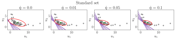
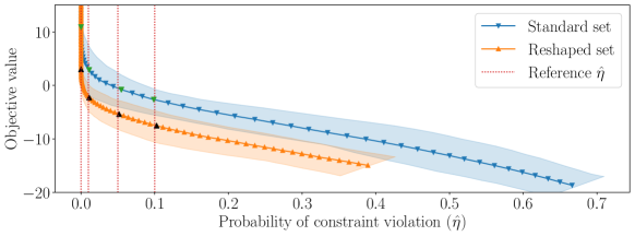
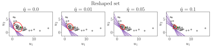
Figure 1: Top: each plot shows the uncertainty set corresponding to the labeled empirical probability of constraint violation, $\hat{\eta}$. White dots: training data points. Green dot: training data mean. Red ellipsoid: standard uncertainty set. Purple lines: lines corresponding to a constraint function value of 0; for each plot, there is a line for each data driven solution $x(\theta,y_{j})$. Middle: out-of-sample tradeoff curves for the objective value vs. empirical probability of constraint violation, averaged across all problem instances. The shaded regions represent the 0.25 to 0.75 quantiles. Each marker corresponds to an $\rho$ value. The uncertainty sets depicted above and below are denoted by the green and black markers, respectively, and achieves the probabilities of constraint violation $\hat{\eta}$ given by the red dotted lines. Bottom: the same plots as the ones on top, for reshaped uncertainty sets.

Reshaped uncertainty set.

Consider now the same set as in (6) with different shape, i.e., ${\mathcal{U}}(\theta)=\left\{u\mid\|A^{\rm re}u+b^{\rm re}\|_{2}\leq\rho\right\}$, where

$$A^{\rm re}=\left[\begin{array}[]{ll}0.79&-0.07\\ 0.30&\phantom{-}0.98\end{array}\right],\quad b^{\rm re}=\left[\begin{array}[]{l}-1.84\\ -2.80\end{array}\right].$$

This set is obtained by reshaping the standard set. In the following sections, we detail the learning procedure to obtain this set.

Comparison.

We now compare the two uncertainty sets where we vary $\rho$ while $A^{\rm st},b^{\rm st}$ and $A^{\rm re},b^{\rm re}$ are fixed. For each value of $\rho$ we compare the average out-of-sample objective value at the optimizers $x(\theta,y)$, where the average is taken across problem instances $y$’s, against the out-of-sample empirical probability of constraint violation, also averaged across instances. Figure 1 shows that the reshaped uncertainty set achieves data-driven solutions that give, on average, better tradeoffs between the out-of-sample objective value and empirical probability of constraint violation. While the standard uncertainty set conforms to the shape of data, it might be conservative because it does not take into account the structure of the optimization problem. In contrast, the reshaped uncertainty set gives better (lower) worst-case costs for the same probability of constraint satisfaction, even though it does not conform as well to the shape of the data. For some target values of empirical probability of constraint violation, $\hat{\eta}$, we plot the constraint values evaluated at $x(\theta,y)$ for all $y$, i.e. the contour lines $k^{T}x(\theta,y)-p^{T}\min\{x(\theta,y),u\}-\tau=0$, for both the standard and reshaped sets. In the top and bottom plots of Figure 1, we notice that although the reshaped set is much smaller than the standard set, it is still tangent to all contour lines corresponding to the constraint value of 0, ensuring that the constraints are satisfied across all instances of $y$. In this way, the optimal uncertainty set is not biased towards a single optimization problem, but instead trained for the entire family of problems parametrized by $y$.

To this end, in this work we propose an automatic technique to obtain the shape and size of the uncertainty sets, parametrized as $\theta$, such that the problem objective is minimized while guaranteeing constraint satisfaction across all members of our problem family.

3 Learning the uncertainty set

3.1 The data-driven problem and bi-level formulation

Suppose we are given a RO problem (1) and a dataset $U^{N}=\{d_{i}\}_{i=1}^{N}\subseteq\mathcal{D}_{u}$ of a set of $N$ independent samples of the uncertain parameter $u$, governed by ${\mathbf{P}}^{N}$, its product distribution. We are also given a dataset $Y^{J}=\{y_{i}\}_{j=1}^{J}\subseteq\mathcal{D}_{y}$ of a set of $J$ independent samples of the family parameter $y$, governed by ${\mathbf{P}}^{J}$, its product distribution. With these datasets, we formulate combined samples $w_{ij}=(d_{i},y_{j})$, which leads to the combined dataset $W_{N\times J}=U^{N}\times Y^{J},$ with product distribution ${\mathbf{P}}^{N\times J}$. We use these datasets to determine the optimal $\theta$, and for which the corresponding $\mathcal{U}(\theta)$ implies a certain finite-sample probabilistic guarantee

$${\mathbf{P}}^{N\times J}\left\{{\mathbf{P}}_{(u,y)}(g(x(\theta,y),u,y)\leq 0)\geq 1-\eta\right\}\geq 1-\beta.$$ (7)

Here, $u$ are realizations of the constructed uncertainty set, $y$ are the family parameters, and ${\mathbf{P}}_{(u,y)}$ denotes the joint distribution of $(u,y)$. In order to formalize the learning task, we define an outer problem minimizing the expected value of the objective function $f(x(\theta,y),y)$ of (1), subject to the following constraint,

$$\mathop{\bf CVaR}(g(x(\theta,y),u,y),\eta)=\kappa,$$

where $\kappa\leq 0$ is a target value, and the $\mathop{\bf CVaR}$ is defined as in (3). As mentioned in Section 2, this then implies a probabilistic guarantee of constraint satisfaction (4). The training problem becomes the $\mathop{\bf CVaR}$ constrained bi-level problem,

$$\begin{array}[]{ll}\mbox{minimize}&{\mbox{\bf E}}_{w}[\ell(z,w)]\\ \mbox{subject to}&{\mbox{\bf E}}_{w}[h(z,w)]=0,\\ \end{array}$$ (8)

where $z=(\theta,\alpha)$, $w=(u,y)$, and,

$$\ell(z,w)=f(x(\theta,y),y), \quad h(z,w)=\frac{(g(x(\theta,y),u,y)-\alpha)_{+}}{\eta}+\alpha-\kappa,$$

and $x(\theta,y)$ are solutions of the lower level problems, defined as

$$\begin{array}[]{lll}x(\theta,y)\in\Phi(\theta,y)=&\underset{x}{\text{argmin }}&f(x,y)\\ &\mbox{subject to}&g(x,u,y)\leq 0\quad\forall u\in{\mathcal{U}}(\theta).\end{array}$$ (9)

The expectation constraint corresponds to the $\mathop{\bf CVaR}$ constraint where $\alpha$ is shifted to become a minimization variable. When the function $\ell$ in the objective is convex, this shift in $\alpha$ has no impact on the optimal solution [SSU08]. With this formulation, we tune $\theta$ and $\alpha$ in the outer level problem depending on the results of the lower level problem, and any set of optimal solutions $x(\theta,y)\in\Phi(\theta,y)$ implicitly depends on the uncertainty set parameterization $\theta$. A good $\theta$ then, should lend solutions $x(\theta,y)$ which performs well with respect to the outer problem. Due to the nonconvex nature of the constraints and the stochasticity of the problem, (8) is difficult to solve. We therefore tackle it using a stochastic augmented Lagrangian method.

3.2 Training the uncertainty set

3.2.1 Augmented Lagrangian method

In order to learn the optimal $z$, we would like to transform the constrained outer function in (8) using the augmented Lagrangian method [NW06, Section 17.3]. For simplicity of notation, from here onwards we adopt the shorthands

$$F(z)={\mbox{\bf E}}_{w}[\ell(z,w)],\quad H(z)={\mbox{\bf E}}_{w}[h(z,w)].$$

We, then, create the unconstrained function

$$L(z,\lambda,\mu)=F(z) +\lambda(H(z))+\frac{\mu}{2}\|H(z)\|^{2},$$

where $\lambda$ and $\mu$ parameters that we update throughout the iterations of the learning algorithm. Our procedure estimates the derivative of $L(z,\lambda,\mu)$ using a subgradient $G(W,z,\lambda,\mu)$ computed over a subset $W$ of the data points. A key component to evaluating this subgradient lies in computing $\nabla_{\theta}x(\theta,y)$. For this we make use of the results [ABB⁺19], which enable us to find gradients of optimal solutions for convex problems by differentiating through the KKT optimality conditions.

The procedure to learn the optimal $z$ is described in Algorithms 1 and 2. Algorithm 1 details the outer level Lagrangian updating procedure for convergence to an $\epsilon$-KKT point in expectation to (8), while Algorithm 2 details obtaining $\epsilon$-stationary points in expectation of $L$. An $\epsilon$-KKT point in expectation is defined as follows.

Definition 3.1 ($\epsilon$-KKT point in expectation [ZZWX22]).

Given $\epsilon>0$, a point $z=(\theta,\alpha)\in{\mbox{\bf R}}^{m\times m}\times{\mbox{\bf R}}^{m}\times{\mbox{\bf R}}$ is an $\epsilon$-KKT point in expectation to (8) if there is a vector $\gamma\in{\mbox{\bf R}}$ such that

$${\mbox{\bf E}}[\|H(z)\|^{2}]\leq\epsilon^{2},\quad{\mbox{\bf E}}[\mathbf{dist}(0,\partial F(z)+J_{H}(z)^{T}\gamma)^{2}]\leq\epsilon^{2},$$

where $J_{H}(z)$ is the Jacobian of function $H$ at $z$.

While these true expectations cannot be computed, we can guarantee the conditions above at convergence [ZZWX22].

Algorithm 1 Stochastic augmented Lagrangian algorithm to solve (8)

1:given $z^{0}=(A^{\text{init}},b^{\text{init}},\alpha^{0})$, $\lambda^{0},\mu^{0},\kappa,\sigma,\gamma_{\rm max},\epsilon$

2:for $k=1,\dots,k_{\rm max}$ do

3:     obtain $z^{k}$ satisfying ${\mbox{\bf E}}[\mathbf{dist}(0,\partial_{z}L(z^{k},\lambda^{k-1},\mu^{k-1}))^{2}]\leq\epsilon^{2}$ $\triangleright$ using Algorithm 2

4:     $\lambda^{k}\leftarrow\lambda^{k-1}+\min\{\mu^{k-1}(H(z^{k})),\gamma_{\rm max}\}$ $\triangleright$ update Lagrange multipliers, with all data

5:     $\mu^{k}\leftarrow\sigma\mu^{k-1}$

6:return $z^{k_{\rm max}}$

For each outer iteration $k$, we call Algorithm 2 with dataset ${W^{k}=U^{k}\times Y^{k}\subseteq W_{N\times J}}$, where $U^{k}\subseteq U^{N}$ and $Y^{k}\subseteq Y^{J}$, sampled uniformly and with overall size $|W^{k}|=M_{1}$. We initialize $\lambda=\lambda^{k-1}$, $\mu=\mu^{k-1}$. The values of $\gamma$, and $\delta$ are initialized as detailed in Appendix A.1. For each subsequent inner iteration $t$, we use subsets $W^{t}$ of the corresponding outer iterations’ datasets, with overall size $|W^{t}|=M_{2}$.

Algorithm 2 Subroutine to obtain $\epsilon$-stationary points in expectation, $z^{k}$, for all $k$

1:given $\hat{z}^{0},\lambda,\mu,\kappa,\gamma,\delta,W,Y$

2:$x^{0}\leftarrow$ solve inner problem (9) over $x$ for $y\in Y$

3:$v^{0}\leftarrow G(W,\hat{z}^{0},\lambda,\mu)$,

4:for $t=1,\dots,t_{\rm max}$ do

5:     sample uniformly datasets $W^{t}\subset W$ and $Y^{t}\subset Y$

6:     $\hat{z}^{t}\leftarrow\hat{z}^{t-1}-\gamma v^{t-1}$

7:     $x^{t}\leftarrow$ solve inner problem (9) over $x$ for all $y\in Y^{t}$

8:     $v_{1}^{t}\leftarrow G(W^{t},\hat{z}^{t-1},\lambda,\mu)$

9:     $v_{2}^{t}\leftarrow G(W^{t},\hat{z}^{t},\lambda,\mu)$

10:     $v^{t}\leftarrow v_{2}^{t}+(1-\delta)(v^{t-1}-v_{1}^{t})$

11:Choose $\hat{z}$ uniformly at random from $\{\hat{z}^{1},\dots,\hat{z}^{t_{\rm max}}\}$

12:return $\hat{z}$

3.2.2 Convergence of the Augmented Lagrangian method

Our formulation fits in the framework of the nonconvex expectation constrained problem of [ZZWX22] and [XX23]. Under standard bounded gradient, smoothness, and regularity conditions, detailed further in Appendix A.1, Algorithm 1 converges to an $\epsilon$-KKT point in expectation to (8). In particular, we require the following regularity condition.

Assumption 3.1 (regularity condition, [ZZWX22, LCL⁺21]).

Given the finite and bounded domain $\Theta$ of the decision variable $z=(\theta,\alpha)$, there exists a constant $v>0$ such that for any $z\in\Theta$,

$$v\|F(z)\|\leq\mathbf{dist}(-J_{H}(z)^{T}H(z),\mathcal{N}_{\Theta}(z)),$$

where $\mathcal{N}_{\Theta}(z)$ is the normal cone of $\Theta$ at $z$, defined as

$$\mathcal{N}_{\Theta}(z)=\{s\mid s^{T}(y-z)\leq 0,\quad\forall y\in\Theta\}.$$

This condition ensures that when the penalty $\mu$ is large, a near-stationary point of the augmented Lagrangian function is near feasible to (8). This assumption is neither stronger or weaker than other common regularity conditions such as the Slater’s condition and the MFCQ condition, and has been proven for many applications [LCL⁺21, SEA⁺19].

We can now give an informal theorem on the convergence of Algorithm 1.

Theorem 3.1 (algorithm convergence (informal)).

Let $\epsilon$ be a small enough positive number. Then, under standard smoothness conditions and regularity Assumption 3.1, Algorithm 1 needs at most $k_{\rm max}$ outer iterations to find an $\epsilon$-KKT point in expectation of (8), where

$$k_{\rm max}=O(\log_{\sigma}(1/\epsilon)).$$

In addition, the number of inner iterations $t^{k}_{\rm max}$ needed by Algorithm 2 is

$$t^{k}_{\rm max}=O(1/\epsilon^{3}).$$

See Appendix A.1 for the exact terms. This result is an application of [ZZWX22, Theorem 1, Theorem 2] and [XX23, Corollary 2].

4 Probabilistic guarantees of constraint satisfaction

To satisfy the probabilistic guarantee (7) for out-of-sample data, we make use of empirical process theory and a covering number argument. We begin with a boundedness assuption on the function $h$, defined in (8).

Assumption 4.1.

The function $h(z,w)$ maps to values in $(-C_{1},C_{2})$, where $0\leq C_{1},C_{2}<\infty$, for all $z,w$ in its support.

We normalize function $h$ by $C=C_{1}+C_{2}$ and define

$$\psi_{s}(u,y)=\frac{1}{C}\left(C_{1}+\frac{(g(x,u,y)-\alpha)_{+}}{\eta}+\alpha\right),$$ (10)

where $s=(x,\alpha)\in{\mbox{\bf R}}^{n+1}$. The function $\psi_{s}$ then maps to values between 0 and 1, and we consider the entire function class

$$\Psi=\{\psi_{s}\}_{s\in\mathcal{S}},$$

where we also impose the following assumption on $\mathcal{S}$. These conditions lead to our finite sample probabilisitc guarantee in Theorem 4.1.

Assumption 4.2.

The set $\mathcal{S}$ is bounded, i.e. ${\mathcal{S}=\{s=(x,\alpha)\in{\mbox{\bf R}}^{n+1}:\|s\|\leq R\}},~{}{0<R<\infty}.$

Theorem 4.1 (Finite sample probabilistic guarantee).

For function class $\Psi$ defined above, if the following condition on the covering number $N$ holds for some constants $V$ and $K$, for all probability measures $Q$ and the $L_{2}(Q)$ norm,

$$\sup_{Q}N(\delta,\Psi,L_{2}(Q))\leq\left(\frac{K}{\delta}\right)^{V},$$ (11)

for every $0<\delta<K,$ then when Algorithm 1 converges to an $\epsilon$-KKT point, we have the finite sample probabilistic guarantee

$${\mathbf{P}}^{N\times J}\left({\mathbf{P}}_{(u,y)}(g(x,u,y)\leq 0)\geq 1-\eta\right)\geq 1-\beta,$$ (12)

where $\beta=(D\sqrt{N}C\tau/\sqrt{V})^{V}\exp(-2NC^{2}\tau^{2})$, $D$ is a constant that depends only on $K$, and $\tau\leq(\kappa+\epsilon)/C$. This is stronger than and implies the probabilistic guarantee given in (7), as it holds for all $x$.

Proof.

By the definition of the function class $\Psi$ and Assumptions 4.2, 4.1, we can apply [vdVW96, Theorem 2.14.9] to get

$${\mathbf{P}}^{N\times J}\left(\sup_{\psi_{s}\in\Psi}\left\|\frac{1}{J}\frac{1}{N}\sum_{j=1}^{J}\sum_{i=1}^{N}\psi_{s}(d_{i},y_{j})-{\mbox{\bf E}}_{(u,y)}[\psi_{s}(u,y)]\right\|\leq\tau\right)\geq 1-\left(\frac{D\sqrt{N}C\tau}{\sqrt{V}}\right)^{V}\exp(-2NC^{2}\tau^{2}).$$

By the convergence of Algorithm 1 to an $\epsilon$-KKT point in expectation, we have that the empirical $\mathop{\bf CVaR}$ will be close to $\kappa$, which given the Equation (10), means

$$\frac{1}{NJ}\sum_{j=1}^{J}\sum_{i=1}^{N}\psi_{s}(d_{i},y_{j})\leq(1/C)(\kappa+\epsilon).$$

Therefore, we have

$${\mathbf{P}}^{N\times J}\left(\sup_{\psi_{s}\in\Psi}{\mbox{\bf E}}_{(u,y)}[\psi_{s}(u,y)]\leq(1/C)(\kappa+\epsilon)+\tau\right)\geq 1-\beta,$$

where $\beta=(D\sqrt{N}C\tau/\sqrt{V})^{V}\exp(-2NC^{2}\tau^{2})$. If $\kappa$ is set such that $(1/C)(\kappa+\epsilon)\leq-\tau$, we then have

$${\mathbf{P}}^{N\times J}\left(\mathop{\bf CVaR}(g(x,u,y),\eta)\leq 0\right)\geq 1-\beta,$$

which implies

$${\mathbf{P}}^{N\times J}\left({\mathbf{P}}_{(u,y)}(g(x,u,y)\leq 0)\geq 1-\eta\right)\geq 1-\beta.$$ (13)

∎

Covering number for $L$-Lipschitz functions.

When $\psi_{s}$ is $L$-Lipschitz in $s$ for all $u$ and $y$, i.e.

$$|\psi_{s}(u,y)-\psi_{s^{\prime}}(u,y)|\leq L\|s-s^{\prime}\|_{2},$$

we can apply standard bounds on the covering number of Lipschitz losses [vdVW96, Pol90, ND17]. In this case, the covering number condition (11) reduces to

$$\sup_{Q}N(\delta,\Psi,L_{2}(Q))\leq N(\delta/L,\mathcal{S},\|\cdot\|_{2})\leq\left(1+\frac{RL}{\delta}\right)^{n+1}\leq\left(\frac{K}{\delta}\right)^{n+1},$$

for every $0<\delta<K$, where $K=\delta+RL$. Then, $\beta=(D\sqrt{N}C\tau/\sqrt{n+1})^{n+1}\exp(-2NC^{2}\tau^{2})$. In practice, affine and max-of-affine $g$ functions fit in this function class.

5 The LROPT package

We introduce the Python package LROPT which builds off CVXPY [DB16] and Cvxpylayers [AAB⁺19], to solve robust optimization problems while learning the optimal parametrization $\theta$ of the uncertainty set. We automatically handle the constraint reformulation process to remove depenency on the uncertain parameter $u$ and set $\mathcal{U}(\theta)$, in order to transform the robust problem 1 into an equivalent convex one. The package is available at:

https://stellatogrp.github.io/lropt.

In each LROPT problem, the user may define the uncertainty set $\mathcal{U}(\theta)$ by electing to either:

1. Explicitly define the parameterization $\theta$ upfront, or

2. Provide a dataset $U^{N}$ of past realizations of $u$, and a set $Y^{J}$ of instances of $y$, leaving $\theta$ to be automatically learned via the procedure described in Section 3.2.1.

As long as the user-specified robust problem follows the defined rules in Section 5.3, LROPT will automatically dualize and solve it. Example formulations are given in Appendices A.2 A.3 with proofs provided in Appendix A.5. For code details and examples, see Section 5.2.

5.1 Uncertainty sets

For ease of use, LROPT is equipped with structure for describing array of common uncertainty sets you might need. For this section, we suppress the dependency of the problem parameter $y$, abbreviating $f(x,y)$ as $f(x)$ and $g(x,u,y)$ as $g(x,u)$ as the $y$’s are fixed data for each problem, and independent of the dualization procedure. As described, every RO problem is written with uncertainty parameter $u$ and an uncertainty set $\mathcal{U}(\theta)$, working together to describe an uncertain constraint as in (1)

$$g(x,u)\leq 0\quad\forall u\in\mathcal{U}(\theta).$$ (14)

Here, we give an example set, and describe its parameterization $\theta$. We leave the description and reformulations of the other supported uncertainty sets to Appendices A.2 and A.3 and the codebase.

Ellipsoidal uncertainty.

Arguably the most common uncertainty sets used in RO is the ellipsoidal uncertainty set, which we write as

$${\mathcal{U}}_{\text{ellip}}(\theta)=\{u\mid\|Au+b\|_{2}\leq 1\},$$

where $\theta=(A,b)$. For a simple affine constraint

$$g(x,u)=(Pu+a)^{T}x,$$ (15)

we obtain the following convex reformulation for the original RO problem.

$$\begin{array}[]{ll}\mbox{minimize}&f(x)\\ \mbox{subject to}&a^{T}x-b^{T}\gamma+\|\gamma\|_{2}\leq 0\\ &A^{T}\gamma=P^{T}x,\\ \end{array}$$ (16)

where $\gamma\in{\mbox{\bf R}}^{m}$ is an auxiliary variable.

5.1.1 Training the sets

To learn the uncertainty set from data, the user provides the datasets $U^{N}$ and $Y^{J}$ to approximate the augmented Lagrangian outer function $L(z,\lambda,\mu)$ detailed in Section 3.2.1. The learning procedure is then handled by pytorch to build a computational graph enabling autograd, in addition to Cvxpylayers [AAB⁺19] to differentiate through the KKT conditions of the inner problem (9). For more details on how Cvxpylayers embeds an optimization problem as a layer in a neural network, see [AK21]. Our package applies the stochastic augmented Lagrangian Algorithm 1, with all parameters user-specifiable, including learning-rate schedulers.

5.2 Automatic canonicalization procedure

One of the core features of LROPT is the novel canonicalization process which converts the human-readable RO problem with uncertain parameters into a convex optimization problem. The procedure is depicted in Figure 2.

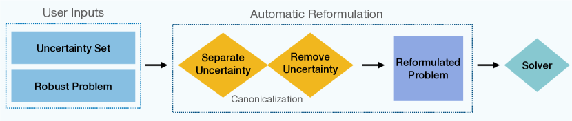
Figure 2: LROPT’s procedure for solving robust problems

The reformulation of the uncertain constraints into a convex CVXPY problem is done via a canonicalization process whose steps are described in more detail in Appendix A.6. To illustrate this process, consider the same $g(x,u)=(Pu+a)^{T}x$ from Equation (15) andthe ellipsoidal uncertainty set $\mathcal{U}_{\text{ellip}}(\theta)=\mathcal{U}_{\text{ellip}}(A,b)=\{u\ |\ ||Au+b||_{2}\leq 1\}$. In LROPT syntax, this problem is described in Listing 3, where $A$ and $b$ could be pre-defined and passed to the uncertainty set.

⬇

x = cp.Variable(n)

u = lropt.UncertainParameter(n,

uncertainty_set=lropt.Ellipsoidal(A=A, b=b))

\parprob = lropt.RobustProblem(cp.Minimize(c @ x),

[(P @ u + a) @ x <= 0])

prob.solve()

Figure 3: LROPT example with fixed uncertainty set parameters $\theta$

If instead we wanted to learn the parameters $(A,b)$, we would import a dataset of previous realizations of the uncertain parameter $u$, then call the ${\tt train}$ function. This procedure is given in Listing 4.

⬇

# data = … datasets for y and u

y = Parameter(n, data=data_y)

u = UncertainParameter(n, uncertainty_set=Ellipsoidal(data=data_u))

\parx = cp.Variable(n)

\parobjective = cp.Minimize(a @ x)

constraints = [x @ u + y @ x <= c]

\parprob = RobustProblem(objective, constraints)

\parprob.train()

prob.solve()

Figure 4: LROPT example for training uncertainty set parameters $\theta$

5.2.1 Procedure overview

By defining $c(u)=||Au+b||_{2},$ we can write the uncertain constraint in Equation (1) as

$$\min_{\lambda\geq 0}\max_{u\in\mathcal{U}}g(x,u)-\lambda(c(u)-1)\leq 0,$$

This constraint can be rewritten as

$$[-g]^{*}(x,z_{1})+[\lambda c]^{*}(z_{2})+\lambda\leq 0,\quad z_{1}+z_{2}=0,$$

where $z_{1},z_{2}$ are new decision variables, and $[-g]^{*}(x,z_{1})$ is the conjugate function of $-g(x,u)$ in parameter $u$ (see Appendix A.5). In terms of the toy constraint, this is equivalent to writing

$$[-g_{1}]^{*}(x,z_{1})+[\lambda c]^{*}(z_{2})+a^{T}x+\lambda\leq 0,\quad z_{1}+z_{2}=0,$$ (17)

where $g_{1}(x,u)=u^{T}P^{T}x$. In essence, LROPT works by in two main steps

1. Separate uncertainty. LROPT breaks down the original uncertain constraint $g(x,u)$ from (1) into a sum of subexpressions with and without uncertain parameters. This way LROPT can to take the appropriate conjugates of the more manageable uncertain subexpressions such as in (17), while ignoring the terms not affected by the uncertainty.

2. Remove uncertainty. LROPT resolves the above conjugate functions in (17) to obtain explicit constraints of the following form,

   $$a^{T}x-b^{T}\gamma+\lambda\leq 0$$

   $$z_{1}=-P^{T}x,\quad_{2}=A^{T}\gamma$$

   $$z_{1}+z_{2}=0,\quad||\gamma||_{2}\leq\lambda,$$

   which simplifies exactly to (16).

5.3 LROPT ruleset

Here we describe a set of rules on the types of functions $g(x,u,y)$ that LROPT can reformulate and solve. Similar to disciplined convex programming (DCP), and disciplined parameterized programming (DPP) rules enforced by Cvxpy [DB16] for solving convex optimization problems, or DSP rules derived from [JN22] and implemented by [SLB23] for solving convex-concave saddle point problems, the LROPT ruleset is necessary for a RO problem to have a convex reformulation, but they are sufficient and indeed cover a broad range of robust problems.

We say that $g(x,u,y)$ is LROPT-compliant if it can be written as a sum of smaller subexpressions

$$g(x,u,y)=\sum_{i=1}^{n}g_{i}(x,u,y),$$ (18)

where each subexpression $g_{i}(x,u,y)$ is DPP in $y$ and either

• DPP in the parameter $u$, and DCP convex in variable $x$

• A non-negative scaling of LROPT atoms described in Section 5.3.1

• A maximum over any number of the previous expressions

Broadly speaking, a RO problem has a convex reformulation if $g(x,u)$ is concave in $u$ and convex in $x$, or is represented by the maximum of expressions which are concave in $u$ and convex in $x$.

5.3.1 LROPT atoms

The LROPT package introduces the following new atoms which are convex in $x$ and concave in $u$.

Matrix-vector product.

The matrix-vector multiplication syntax @ is supported for writing affine expressions in $u$ such as x@P@u.

Quadratic form.

The atom $\tt{quad\_form(u,A*x)}$ represents the function $g_{i}(x,u)=(u^{T}Au)x$ where $A\in{\mbox{\bf R}}^{m\times m}$, $A\preceq 0$, and $x\in{\mbox{\bf R}}$ is a scalar variable multiplying the quadratic form.

Weighted log-sum-exp.

The atom $\tt{log\_sum\_exp}(u,x)$ represents the function $\log\left(\sum_{i=1}^{n}u_{i}e^{x_{i}}\right)$. Here $x\in{\mbox{\bf R}}^{m}$, and $u\in{\mbox{\bf R}}^{m}$ must be of the same dimension.

Weighted $l_{2}$ norm.

The atom $\tt{weighted\_norm2}$ represents the function $\left(\sum_{i=1}^{n}u_{i}x_{i}^{2}\right)^{\frac{1}{2}}$. Again $x\in{\mbox{\bf R}}^{m}$, and $u\in{\mbox{\bf R}}^{m}$ must be of the same dimension.

Matrix quadratic form.

The atom $\tt{mquad\_form(U,x)}$ reprsents the function $g(x,u)=x^{T}Ux$ where $U\succeq 0$, is constrained by LROPT to be PSD.

5.3.2 Multiple uncertain constraints

LROPT allows for expressing multiple uncertain constraints as a single maximum of concave constraint. In particular, given a set of constraints

$$g_{l}(x,u,y)\leq 0,\quad l=1,\dots,L,$$

where each $g_{l}$ satisfies the ruleset defined above, we can write a single joint uncertain constraint,

$$g(x,u,y)=\max_{l}g_{l}(x,u,y)\leq 0,$$ (19)

as the joint constraint is still complient of the ruleset. We also allow for disjoint constraints. In this case, a separate $h$ can be defined for each uncertain constraint, and the expectation constraint in (8) and the corresponding multiplier $\lambda$ becomes vector-valued.

5.4 Default training parameters

Algorithms 1 and 2 rely on various parameters that the user can specify. We set the default values as follows:

1. The reshaping parameters $\theta=(A,b)$ are initialized as $A=\hat{\Sigma}^{-1/2}$, $b=-A\hat{\mu}$, where $\hat{\Sigma}$ is the empirical standard deviation of the data, and $\hat{\mu}$ is the empirical mean.

2. The $\mathop{\bf CVaR}$ parameters are: risk $\eta=0.05$ and target value $\kappa=-0.015$. The initial value of the $\mathop{\bf VaR}$ proxy is $\alpha^{0}=0$.

3. The Lagrangian multipliers and penalty are initialized as $\lambda^{0}=0$ and $\mu^{0}=1$. The penalty update is $\sigma=1.01$, and the maximum $\lambda$ update value is $\gamma_{\rm max}=100$.

4. The subsets of the training data used at each iteration have sizes $M_{1}=NJ$, $M_{2}=NJ/10$.

5. We use $t_{\rm max}=10$ inner iterations and $k_{\rm max}=1000$ outer iterations.

6. We set the step sizes to $\gamma=0.0001$ and $\delta=0.01$.

6 Examples

The following experiments are run on an M1 Macbook with 8 GB memory. The learning procedure relies on the Python package Cvxpylayers [AAB⁺19], and is implemented using the LROPT package. The code can be accessed at

https://github.com/stellatogrp/lropt/.

For each experiment, we compare the following methods.

Standard RO.

We perform standard RO, where the shape of the uncertainty set is determined by the empirical mean and variance of the data [BTN00]. We use grid search to find the size parameter $\rho$ that gives an in-sample empirical probability of contraint violation of 0.03.

Wasserstein DRO.

We also perform Wasserstein DRO [EK18], where the uncertainty set is constructed around individual data points. We again use grid search to find the size parameter $\rho$ that gives an in-sample empirical probability of constraint violation of 0.03.

LROPT.

For LROPT, we apply the training method given in Section 3.2.1, with parameters set as in Section 5.4. The step sizes $\gamma$ are chosen problem-wise.

LROPT + Fine Tuning.

Upon completion of the LROPT training procedure, we also fine tune the size of the uncertainty set using grid search to achieve an in-sample empirical probability of contraint violation of 0.03.

For each setting, we repeat the experiment 100 times, each with a new independent dataset. For each method, we evaluate the performance metrics in Table 1.

Table 1: Performance metrics in numerical examples, averaged over 100 runs.

Name	Description
Obj.	Objective value estimate for problem (8)
$\hat{\eta}$	Out-of-sample empirical probability of constraint violation
$\hat{\beta}$	Estimated confidence, given as ${\mathbf{P}}(\hat{\eta}>\eta)$
Time	Average solution time of the final robust problem after training

6.1 Portfolio management

Problem description.

We consider the classic portfolio management problem where we select a portfolio $x\in{\mbox{\bf R}}^{n}$ of stocks to maximize returns. Our selected stock should not deviate too far from our previous holdings, denoted $x^{\text{prev}}\in{\mbox{\bf R}}^{n}$. We parametrize the optimization problem by $y=x^{\text{prev}}$, obtaining the followig RO formulation

$$\begin{array}[]{ll}\mbox{minimize}&t+\eta\|x-x^{\text{prev}}\|_{1}\\ \mbox{subject to}&-u^{T}x\leq t\quad\forall u\in{\mathcal{U}}(\theta)\\ &\mathbf{1}^{T}x=1,\quad x\geq 0.\end{array}$$

Therefore, the uncertain constraint is

$$g(t,x,u,x^{\text{prev}})=-u^{T}x-t\leq 0,\quad\forall u\in{\mathcal{U}}(\theta).$$

Data.

We set $n=15$ stocks and $N=500$ data points for both the training and testing sets. We generate uncertain returns $u$ from 3 normal distributions, to simulate 3 uncertain market environments. For distribution $l$, $\mu_{i}=0.1+\gamma_{l}0.05i$ for all $i=1,\dots,f$, with scaling parameters $\gamma=(1,2,3)$. The variance is $\sigma_{i}=0.02^{2}+(0.08i)^{2}$ for all distributions. This means that the higher the index of the stock, the higher returns and higher variance it has. To enforce holdings summing up to $1$, we set each instance of the previous holdings $x^{\text{prev}}$ using the Dirichlet distribution, with parameter value $(2.5,1,.5,.5,.4,.3,.3,.2,.2,.15,.1,.1,.1,.1,.1)$, corresponding to the 15 different stocks. The decreasing values by index indicate less holdings of the riskier stocks.

Results.

In Table 2, we compare the performance of our LROPT method with standard RO and Wasserstein DRO, as described in the beginning of this section. We note that the final learned reshaped uncertainty set achieves a low empirical probability of constraint violation while also ensuring a low out-of-sample objective value. In comparsion, standard RO and Wasserstein DRO provides worse trade-offs.

Table 2: Portfolio management: comparing the performance of various methods, averaged across 100 iterations. LROPT: learing the shape of the uncertainty set. LROPT + Fine Tuning: tuning the size of the learned uncertainty set. RO: standard RO where only the size is tuned. Wass. DRO: Wasserstein DRO. For the last three methods, the in-sample empirical probability of constraint violation are tuned to be 0.03. Obj.: the average out-of-sample objective value. Time: final solve-time once the uncertainty sets are constructed, not including training time. For all methods, the same number of data points for testing and training is used.

Method	LROPT	LROPT + Fine Tuning	RO	Wass. DRO
[head to column names]./images/table_vals.csv

In Figure 5, for one of the 100 runs of the experiment, we show the trade-off between the average objective value and empirical probability of constraint violation for the standard and reshaped uncertainty sets. The graphs are obtained by varying the size $\rho$ of the two sets. We notice that the tradeoff improves for the reshaped sets.

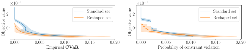
Figure 5: Left: average out-of-sample objective values versus empirial $\mathop{\bf CVaR}$ for both parametrizations of the uncertainty set, for one run of the experiment. This graph is obtained by varying the $\rho$ value (size) for both the standard and reshaped sets. The average is taken across all problem instances, and the shaded region represents the 0.1 to 0.9 quantiles. Right: average out-of-sample objective values versus empirical probability of constraint violation, for one run of the experiment.

6.2 Multi-product newsvendor

Problem description.

We consider a newsvendor problem where two series of correlated products are sold in conjuction. When both series are available, they will be sold as a set, and when only series one (the main product) is available, only that series will be sold. For simplicty, we allow fractional orders. At the beginning of each day, the vendor produces $x_{1}\in{\mbox{\bf R}}^{n}$ products of the first series, and $x_{2}\in{\mbox{\bf R}}^{n}$ products of the second series, with respective costs $k_{1}\in{\mbox{\bf R}}^{n}$. $k_{2}\in{\mbox{\bf R}}^{n}$. As the supplementary products (series two) will not be sold on their own, we must have $x_{1}\geq x_{2}$. These products will be sold at the prices $p_{1}>k_{1},p_{2}>k_{2}$, until either the demand $u$ or inventory $x$ is exhausted. We parametralize the problem with $y=p_{1}$. For each problem instance, the total cost to minimize is then

$$c(x)=k_{1}^{T}x_{1}-p_{1}^{T}\min\{x_{1},u\}+k_{2}^{T}x_{2}-p_{2}^{T}\min\{x_{2},u\}.$$

Given a historical set of uncertain demands, we solve the data-driven RO problem

$$\begin{array}[]{ll}\mbox{minimize}&\tau+\tau_{1}\\ \mbox{subject to}&k_{1}^{T}x_{1}-p_{1}^{T}\min\{x_{1},u\}\leq\tau\quad\forall u\in{\mathcal{U}}(\theta)\\ &k_{2}^{T}x_{2}-p_{2}^{T}\min\{x_{2},u\}\leq\tau_{1}\quad\forall u\in{\mathcal{U}}(\theta)\\ &x_{1}\geq x_{2}\geq 0.\end{array}$$

As there are two uncertain constraints, we model it as a single maximum of concave constraints as in (19). Specifically, we have

$$g(x_{1},x_{2},u,p_{1})=\max(k_{1}^{T}x_{1}-p_{1}^{T}\min\{x_{1},u\}-\tau,k_{2}^{T}x_{2}-p_{2}^{T}\min\{x_{2},u\}-\tau_{1})\leq 0.$$

Data.

We set $n=15$, and $N=300$ data points for both the training and testing sets. We generate $k_{1}\in{\mbox{\bf R}}^{n}$ uniformly on $[2,5]$, and $k_{2}\in{\mbox{\bf R}}^{n}$ uniformly on $[1,3]$. The retail prices $p_{1}\in{\mbox{\bf R}}^{n}$ are set as $k_{1}+r_{1}^{\prime}$, where $r_{1}^{\prime}\in{\mbox{\bf R}}^{n}$ is generated uniformly on $[1,3]$, and $p_{2}\in{\mbox{\bf R}}^{n}$ is similarly set as $k_{2}+r_{2}^{\prime}$, where $r_{2}^{\prime}\in{\mbox{\bf R}}^{n}$ is generated uniformly on $[0,2]$. We consider 5 problem instances, where the retail price $p_{1}$ is slightly perturbed. For each instance $j$, we let $y_{j}=p_{1j}=p_{1}+s_{j}$, where $s_{j}$ follows a normal distribution with mean $0$ and standard deviation $1$. The unknown demand is distributed as a log-normal distribution, where the normal distribution has $\mu\sim U[-0.2,2]^{n}$ and $\Sigma=0.1FF^{T}$, where $F\in{\mbox{\bf R}}^{n\times 2}$ has elements drawn from the standard normal distribution.

Results.

In Table 3, we again compare the performance of our LROPT methods with Wasserstein DRO, and note that the reshaped uncertainty set outperforms the others. Visualising the performance of the learned uncertainty sets for one run of the experiment, we observe in Figure 6 that the tradeoff between the average objective value and empirical probability of constraint satisfaction is much better for the reshaped set, thus motivating our approach.

Table 3: Newsvendor: comparing the performance of various methods, averaged across 100 iterations. LROPT: learing the shape of the uncertainty set. LROPT + Fine Tuning: tuning the size of the learned uncertainty set. RO: standard RO where only the size is tuned. Wass. DRO: Wasserstein DRO. For the last three methods, the in-sample empirical probability of constraint violation are tuned to be 0.03. Obj.: the average out-of-sample objective value. Time: final solve-time once the uncertainty sets are constructed, not including training time. For all methods, the same number of data points for testing and training is used.

Method	LROPT	LROPT + Fine Tuning	RO	Wass. DRO
[head to column names]./images/table_vals3.csv

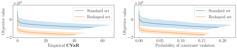
Figure 6: Left: average out-of-sample objective values versus empirial $\mathop{\bf CVaR}$ for both parametrizations of the uncertainty set, for one run of the experiment. The average is taken across all problem instances, and the shaded region represents the 0.1 to 0.9 quantiles. Right: average out-of-sample objective values versus probability of constraint violation, for one run of the experiment.

6.3 Inventory management

We implement an adjusted version of the inventory management example from [IT14][Section 5.2.1.], a two-stage adjustable RO problem. Instead of the deterministic polyhedral uncertainty set considered there, we assume the uncertainty set to be ellipsoidal, with parameters to be learned from data.

Problem description.

We consider a retail network consisting of a single warehouse and $n$ different retail points, indexed by $i=1,\dots,n$. For simplicity, only a single product is sold. There are a total of $C$ units of the product available, and each retail point holds $0$ inventory and is capable of stocking at most $c_{i}$ units. The transportation costs for distributing the items at the $i$th retail point is $t_{i}$ currency units per unit of inventory, and the operating cost is $h_{i}$ per unit. The revenues per unit is $r_{i}$, and customer demand is uncertain, with a nominal demand plus an additional amount dependent on $f$ market factors. The formula for the demand at retail point $i$ is

$$a_{i}=\bar{a}_{i}+q_{i}^{T}u,$$

where $\bar{a}_{i}\in{\mbox{\bf R}}$ denotes the nominal demand, and $q_{i}\in{\mbox{\bf R}}^{f}$ denotes the exposure of demand $a_{i}$ to the market factors. We denote with $u$ the unknown market factors, which belong to an uncertainty set ${\mathcal{U}}(\theta)$. The decision variable is the stocking decisions for all retail points, denoted $s\in{\mbox{\bf R}}^{n}$. In addition, the problem involves a vector $w(u)$ of realized sales at each point, which is dependent on stocking decision $s$ and the unknown factors $u$ affecting the demand. We have

$$w_{i}(u)=\min\{s_{i},a_{i}\},$$

for each retail point. The manager makes stocking decisions to maximize worst-case profits, which is equivalent to minimizing worst-case loss, denoted as $P$. We parametralize the problem with $y=r$. For each problem instance, the RO formulation is given as

$$\begin{array}[]{ll}\mbox{minimize}&P\\ \mbox{subject to}&-r^{T}w(u)+(t+h)^{T}s\leq P,\quad\forall u\in{\mathcal{U}}(\theta)\\ &w_{i}(u)\leq s_{i},\quad i=1,\dots,n,\quad\forall u\in{\mathcal{U}}(\theta)\\ &w_{i}(u)\leq\bar{a_{i}}+q_{i}^{T}u,\quad i=1,\dots,n,\quad\forall u\in{\mathcal{U}}(\theta)\\ &\mathbf{1}^{T}s=C\\ &0\leq s\leq c,\\ \end{array}$$ (20)

where variables $s\in{\mbox{\bf R}}^{n}$, $w\in{\mbox{\bf R}}^{n}$, and $P\in{\mbox{\bf R}}$. To solve this, we first replace the adjustable decision $w_{i}(u)$ with their affine adjustable robust counterparts $z^{0}_{i}+v_{i}^{T}u$, where $z^{0}_{i}\in{\mbox{\bf R}}$ and $v_{i}\in{\mbox{\bf R}}^{f}$ are auxiliary introduced as part of the linear decision rules [BTEGN09]. The new formulation is

$$\begin{array}[]{ll}\mbox{minimize}&P\\ \mbox{subject to}&-r^{T}z^{0}-r^{T}Vu+(t+h)^{T}s\leq P,\quad\forall u\in{\mathcal{U}}(\theta)\\ &z^{0}_{i}+v_{i}^{T}u\leq s_{i},\quad i=1,\dots,n,\quad\forall u\in{\mathcal{U}}(\theta)\\ &z^{0}_{i}+v_{i}^{T}u\leq\bar{a_{i}}+q_{i}^{T}u,\quad i=1,\dots,n,\quad\forall u\in{\mathcal{U}}(\theta)\\ &\mathbf{1}^{T}s=C\\ &0\leq s\leq c,\\ \end{array}$$ (21)

where $V=[v_{1},\dots,v_{N}]^{T}$. As there are multiple uncertain constraints, we again apply a maximum of concave formulation as in Section 5.3.2.

Data.

As in [IT14], we consider the case where $n=10$, and $C=2000$. All other problem data are independently sampled from uniformly distributed random variables. Inventory capacities are between 300 and 500. Transportation and operation costs are between 1 and 3. Sales revenues $r$ are between 20 and 40, and nominal demand values are between 100 and 200. We consider 5 instances for $r$, perturbing each by $r_{j}^{{}^{\prime}}$, where $r_{j}^{{}^{\prime}}$ follows a normal distribution with mean 0 and standard deviation 0.1. The number of market factors $f$ is 4, and exposure parameters $Q$ are between $-2$ and 2. We generate uncertain market factors $u$ from 3 normal distributions, to simulate 3 uncertain market environments. For distribution $j$, $\mu_{i}=\gamma_{j}0.3i$ for all $i=1,\dots,f$, with scaling parameters $\gamma=(1,2,3)$. The variance is $\sigma_{i}=0.02^{2}+(0.1i)^{2}$ for all distributions. The total training sample size is $N=300$, with 100 data points from each distribution. The testing sample size is the same. We assume the uncertainty set to be ellipsoidal, with norm $p=2$.

Results.

In Table 4, we compare the performance of our LROPT method with standard RO and Wasserstein DRO, and again note the desirable tradeoff given by our learned reshaped set.

Table 4: Inventory management: comparing the performance of various methods, averaged across 100 iterations. LROPT: learing the shape of the uncertainty set. LROPT + Fine Tuning: tuning the size of the learned uncertainty set. RO: standard RO where only the size is tuned. Wass. DRO: Wasserstein DRO. For the last three methods, the in-sample empirical probability of constraint violation are tuned to be 0.03. Obj.: the average out-of-sample objective value. Time: final solve-time once the uncertainty sets are constructed, not including training time. For all methods, the same number of data points for testing and training is used.

Method	LROPT	LROPT + Fine Tuning	RO	Wass. DRO
[head to column names]./images/table_vals2.csv

In Figure 7, for one of the 100 runs of the experiment, we again show the trade-off between the average objective value and empirical probability of constraint violation for the standard and reshaped uncertainty sets, and observe an improved trade-off for the reshaped set.

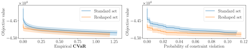
Figure 7: Left: average out-of-sample objective values versus empirial $\mathop{\bf CVaR}$ for both parametrizations of the uncertainty set, for one run of the experiment. The average is taken across all problem instances, and the shaded region represents the 0.1 to 0.9 quantiles. Right: average out-of-sample objective values versus probability of constraint violation, for one run of the experiment.

Appendix A Appendices

A.1 Convergence

We state, for completeness, key assumptions required for the convergence result. In particular, we give the boundedness, smoothness, and unbiasedness assumptions applied to our context. For more details, refer to [ZZWX22].

Assumption A.1 (structured bounded domain).

The domain $\Theta$ of the decision variables $z=(\theta,\alpha)$ must be compact. In addition, there must exist finite constants $B_{0}$ and $B_{h}$ such that

$$B_{0}\geq\max_{z\in\Theta}\max\{|F(z)|,\|\nabla F(z)\|\},\quad B_{h}\geq\max_{z\in\Theta}\|J_{H}(z)\|$$

Assumption A.2 (mean-squared smoothness,  [ZZWX22]).

For any ${z_{1},z_{2}=(\theta_{1},\alpha_{1}),(\theta_{2},\alpha_{2})\in\Theta}$, the functions $\ell(\cdot,w)$ and $h(\cdot,w)$ satisfy the mean-squared smoothness conditions:

$${\mbox{\bf E}}_{w}[\|\nabla\ell(z_{1},w)-\nabla\ell(z_{2},w)\|^{2}]\leq L^{2}_{0}\|z_{1}-z_{2}\|^{2},$$

$${\mbox{\bf E}}_{w}[\|J_{{h}}(z_{1},w)-J_{{h}}(z_{2},w)\|^{2}]\leq L^{2}_{J}\|z_{1},z_{2}\|^{2},$$

$${\mbox{\bf E}}_{w_{1},w_{2}}[\|J_{h}(z_{1},w_{1})^{T}{h}(z_{1},w_{2})-J_{{h}}(z_{2},w_{1})^{T}{h}(z_{2},w_{2})\|^{2}]\leq L^{2}_{J}\|z_{1}-z_{2}\|^{2},$$

where $w_{1}$ and $w_{2}$ are independent and drawn from ${\mathbf{P}}_{u}\times{\mathbf{P}}_{y}$.

Assumption A.3 (unbiasedness and bounded variance [ZZWX22]).

For any $z=(\theta,\alpha)\in\Theta$, the objective and constraints satisfy

$${\mbox{\bf E}}_{w}[\nabla\ell(z,w)]=\nabla F(z),\quad{\mbox{\bf E}}_{w}[J_{h}(z,w)]=J_{H}(z).$$

Also, there exists $\sigma_{f},\sigma_{h}>0$ such that for any $z=(\theta,\alpha)\in\Theta$,

$${\mbox{\bf E}}_{w}[\|\nabla\ell(z,w)-F(z)\|^{2}]\leq\sigma_{f}^{2},\quad{\mbox{\bf E}}_{w}[\|J_{h}(z,w)-J_{H}(z)\|^{2}]\leq\sigma_{h}^{2},$$

$${\mbox{\bf E}}_{w_{1},w_{2}}[\|J_{h}(z,w_{1})^{T}h(z,w_{2})-J_{H}(z)^{T}H(z)\|^{2}]\leq\sigma_{h}^{2},$$

where $(w_{1})$ and $(w_{2})$ are independent and drawn from $\mathbf{P_{u}}\times\mathbf{P_{y}}$.

Under these assumptions, we achieve convergence results detailed in Theorem A.1.

Theorem A.1.

Let $\epsilon$ be such that $\epsilon\leq C_{1}\frac{3\sqrt{\sigma^{2}_{f}+\mu_{0}^{2}\sigma_{h}^{2}}}{10}$. Then, under Assuptions 3.1, A.1, A.2, and A.3, Algorithm 1 needs at most $k_{\rm max}$ outer iterations to find an $\epsilon$-KKT point in expectation of (8), where

$$k_{\rm max}=\max\left\{\left\lceil\log_{\sigma}\frac{\sqrt{8}\sqrt{\epsilon^{2}+B_{0}^{2}}}{\mu_{0}v\epsilon}\right\rceil,\left\lceil 2\log_{\sigma}\frac{\sqrt{8}B_{h}\gamma_{\rm max}}{\mu_{0}v\epsilon}\right\rceil\right\}+1,$$

and $\gamma_{\rm max}$ is large enough such that it satisfies $\frac{\sqrt{8}B_{h}\gamma_{\rm max}}{\mu_{0}v\epsilon}\geq\frac{8}{\ln{\sigma}}.$ In addition, the number of inner iterations $t^{k}_{\rm max}$ needed is at most

$$t^{k}_{\rm max}=\left\lceil\frac{C_{2}\left(\frac{L_{k}(L(z^{k},\lambda^{k},\mu^{k})-L^{k*})_{1+}}{\gamma_{k}}+\frac{\sigma_{k}^{2}}{20c_{0,k}\gamma_{k}^{2}}+\frac{24^{2}\sigma_{K}^{2}\gamma_{k}^{2}}{10M_{2}}\right)^{3/2}}{\epsilon^{3}}\right\rceil,$$

where

$$L_{k}=\sqrt{3L_{0}^{2}+3L_{J}^{2}\|\lambda_{k}\|^{2}+3\mu_{k}^{2}L_{J}^{2}},\quad\sigma_{k}=\sqrt{3\sigma_{f}^{2}+3\sigma_{h}^{2}\|\lambda_{k}\|^{2}+3\mu_{k}^{2}\sigma_{h}^{2}},$$

$$\bar{\gamma}_{k}=\frac{\gamma_{k}}{L_{k}{t^{k}_{\rm max}}^{1/3}},\quad\delta_{k}=\frac{4\gamma_{k}^{2}/M_{2}+10\gamma_{k}^{2}(2-\gamma_{k}{t^{k}_{\rm max}}^{(-1/3)})}{{t^{k}_{\rm max}}^{2/3}+4\gamma_{k}^{2}/M_{2}},$$

$$\gamma_{k}=C_{3}\frac{(L_{k}(L(z^{k},\lambda^{k},\mu^{k})-L^{k*})_{1+})^{(1/3)}}{\sigma_{k}^{2/3}},c_{0,k}=C_{4}\frac{\sigma_{k}^{2/3}}{20(L_{k}(L(z^{k},\lambda^{k},\mu^{k})-L^{k*})_{1+})^{4/3}}.$$

Here, $C_{1},C_{2},C_{3},C_{4}$ are constants, $(a)_{1_{+}}$ represents $\max\{a,1\}$, and $L^{k*}=\min_{z}L(z,\lambda^{k},\mu^{k})$. The expression $(L(z^{k},\lambda^{k},\mu^{k})-L^{k*})_{1+}$ can be upper bounded by known quantities. See the exact constants and bounds in [ZZWX22, Theorem 1, Theorem 2] and [XX23, Corollary 2].

A.2 Uncertainty sets and general reformulations

We introduce some common uncertainty sets, and derive reformulations of (1) for general constraints $g$. As using a reshaping matrix for $u$ can be more powerful than specifying the size of the uncertainty set, we include in $\theta$ the reshaping parameters $(A,b)$. Reformulations for linear constraints are in Appendix A.3, and proofs are in Appendix A.5. We suppress the dependency of $g$ on $y$ here and for all following sections on reformulations.

We consider two general types of functions $g$: the sum of concave functions,

$$g(x,u)=\sum_{j=1}^{J}g_{j}(u,x),$$

where each $g_{j}$ is concave in $u$, and the maximum of affine functions,

$$g(x,u)=\max_{l=1,\dots,L}(P_{l}u+a_{l})^{T}x.$$

Box uncertainty.

The box uncertainty set is defined as

$${\mathcal{U}}_{\text{box}}(\theta)=\{u\mid\|Au+b\|_{\infty}\leq 1\},$$

where $\theta=(A,b)$. Note that if $A=(1/\rho)I$ and $b=0$, this is equivalent to the traditional box uncertainty set ${\{u\mid\|u\|_{\infty}\leq\rho\}}$. For the two types of constraints, we have the following reformulations. The proofs are in Appendix A.5.2. Sum of concave:

$$\begin{array}[]{ll}\mbox{minimize}&f(x)\\ \mbox{subject to}&\sum_{j=1}^{J}[-g_{j}]^{*}(x,z_{j})+b^{T}\gamma+\|\gamma\|_{1}\leq 0,\\ &A^{T}\gamma=z\\ &\sum_{j=1}^{J}z_{j}=z,\end{array}$$ (22)

with auxiliary variables $\gamma,z,z_{j}\in{\mbox{\bf R}}^{m}$, for $j=1,\dots,J$, and $g^{*}(x,z)$ the conjugate of $g(x,u)$ in $u$, evaluated at point $z$. This result follows from the theorem of infimal convolutions for conjugate functions [RW98]. Max of affine:

$$\begin{array}[]{ll}\mbox{minimize}&f(x)\\ \mbox{subject to}&a_{l}^{T}x-b^{T}\gamma_{l}+\lambda\leq 0,\quad l=1,\dots,L\\ &\lambda\geq\|\gamma_{l}\|_{1},\quad l=1,\dots,L\\ &A^{T}\gamma_{l}=P_{l}^{T}x,\quad l=1,\dots,L.\\ \end{array}$$ (23)

Ellipsoidal uncertainty.

The ellipsoidal uncertainty set is defined as

$${\mathcal{U}}(\theta)=\{u\mid\|Au+b\|_{p}\leq 1\},$$

where $\theta=(A,b,p)$. We let $p$ be the order of the norm, which is any integer value $\geq 1$. For the two types of constraints, we have the following reformulations. The proofs are in Appendix A.5.2. Sum of concave:

$$\begin{array}[]{ll}\mbox{minimize}&f(x)\\ \mbox{subject to}&\sum_{j=1}^{J}[-g_{j}]^{*}(x,z_{j})+b^{T}\gamma+\|\gamma\|_{q}\leq 0,\\ &A^{T}\gamma=z\\ &\sum_{j=1}^{J}z_{j}=z,\end{array}$$ (24)

which is the same as the box uncertainty case, with dual norm $q$ instead of $1$. Max of affine:

$$\begin{array}[]{ll}\mbox{minimize}&f(x)\\ \mbox{subject to}&a_{l}^{T}x-b^{T}\gamma_{l}+\lambda\leq 0,\quad l=1,\dots,L\\ &\lambda\geq\|\gamma_{l}\|_{q},\quad l=1,\dots,L\\ &A^{T}\gamma_{l}=P_{l}^{T}x,\quad l=1,\dots,L.\\ \end{array}$$ (25)

Budget uncertainty.

The budget uncertainty set requires both box and ellipsoildal constraints, and is defined as

$${\mathcal{U}}_{\text{bud}}(\theta)=\{u\mid\|A_{1}u+b_{1}\|_{\infty}\leq\rho_{1},\|A_{2}u+b_{2}\|_{1}\leq\rho_{2}\},$$

where $\theta=(A_{1},b_{1},A_{2},b_{2},\rho_{1},\rho_{2})$. For the two types of constraints, we have the following reformulations. The proofs are in Appendix A.5.3. Sum of concave:

$$\begin{array}[]{ll}\mbox{minimize}&f(x)\\ \mbox{subject to}&\sum_{j=1}^{J}[-g_{j}]^{*}(x,z_{j})-b_{1}^{T}\gamma_{1}+b_{2}^{T}\gamma_{2}+\rho_{1}\|\gamma_{1}\|_{1}+\rho_{2}\|\gamma_{2}\|_{\infty}\leq 0,\\ &A^{T}\gamma_{1}=y-z,\quad A^{T}\gamma_{2}=y\\ &\sum_{j=1}^{J}z_{j}=z,\end{array}$$ (26)

with $z,\gamma_{1},\gamma_{2},z_{j}\in{\mbox{\bf R}}^{m}$ for $j=1,\dots,J$ as auxiliary variables. Max of affine:

$$\begin{array}[]{ll}\mbox{minimize}&f(x)\\ \mbox{subject to}&a_{l}^{T}x-b_{1}^{T}\gamma_{1l}+b_{2}^{T}\gamma_{2l}+\rho_{1}\lambda_{1}+\rho_{2}\lambda_{2}\leq,0\quad l=1,\dots,L\\ &\lambda_{1}\geq\|\gamma_{l1}\|_{1},\quad l=1,\dots,L\\ &\lambda_{2}\geq\|\gamma_{l2}\|_{\infty},\quad l=1,\dots,L\\ &A^{T}\gamma_{l1}=y_{l}+P_{l}^{T}x,\quad A^{T}\gamma_{l2}=y_{l},\quad l=1,\dots,L.\\ \end{array}$$ (27)

Polyhedral uncertainty.

The polyhedral uncertainty set is defined as

$${\mathcal{U}}(\theta)=\{u\mid Du\leq d\},$$

where $\theta=(D,d)$ defines the polyhedron. As the polyhedral set is already of a defined shape, we do not add the parameters $(A,b)$. For the two types of constraints, we have the following reformulations. The proofs are in Appendix A.5.4. Sum of concave:

$$\begin{array}[]{ll}\mbox{minimize}&f(x)\\ \mbox{subject to}&\sum_{j=1}^{J}[-g_{j}]^{*}(x,y_{j})+d^{T}z\leq 0,\\ &D^{T}z=-y\\ &\sum_{j=1}^{J}y_{j}=y\\ &z\geq 0,\end{array}$$ (28)

with auxiliary variables $y,y_{j}\in{\mbox{\bf R}}^{m}$ for $j=1,\dots,J$. Max of affine:

$$\begin{array}[]{ll}\mbox{minimize}&f(x)\\ \mbox{subject to}&a_{l}^{T}x+d^{T}z_{l}\leq 0,\quad l=1,\dots,L\\ &D^{T}z_{l}=P_{l}^{T}x,\quad l=1,\dots,L\\ &z_{l}\geq 0,\quad l=1,\dots,L\end{array}$$ (29)

Mean robust uncertainty.

The Mean Robust Uncertainty (MRO) [WBVPS22] set, which is a more general form for Wasserstein DRO, is defined as

$${\mathcal{U}}_{\text{mro}}(\theta) =\left\{u=(v_{1},\dots,v_{K})\quad\middle|\quad\sum_{k=1}^{K}w_{k}\|A_{k}(v_{k}-\bar{d}_{k})\|_{p}^{\rho}\leq 1\right\},$$

where $\theta=(A,\rho,U^{N})$, with $U^{N}$ a dataset of $N$ samples. We partition ${\mathcal{D}}_{N}$ into $K$ disjoint subsets, and $\bar{d}_{k}$ is the centroid of the $k$th subset. The weight we place upon each subset is $w_{k}$, and is equivalent to the proportion of points in the subset. We choose $\rho$ to be an integer exponent, and $p$ to be an integer norm.

For the two types of constraints, we have the following reformulations. The proofs are in Appendix A.5.5. Sum of concave:

$$\begin{array}[]{ll}\text{minimize }&f(x)\\ \mbox{subject to}&\lambda+\sum_{k=1}^{K}w_{k}s_{k}\leq 0\\ &\sum_{j=1}^{J}[-g_{j}]^{*}(x,y_{kj})-z_{k}^{T}A_{k}\bar{d}_{k}+\phi(r)\lambda\left\|\gamma_{k}/\lambda\right\|^{r}_{q}\leq s_{k},\quad k=1,\dots,K\\ &A_{k}^{T}\gamma_{k}=z_{k},\quad k=1,\dots,K\\ &\sum_{j=1}^{J}y_{kj}=z_{k},\quad k=1,\dots,K\\ &\lambda\geq 0,\end{array}$$ (30)

with auxiliary variables $\gamma_{k}\in{\mbox{\bf R}}^{m},z_{k}\in{\mbox{\bf R}}^{m},y_{kj}\in{\mbox{\bf R}}^{m}$ for $j=1,\dots,J$, $k=1,\dots,K$. Max of affine:

$$\begin{array}[]{ll}\text{minimize }&f(x)\\ \mbox{subject to}&\lambda+\sum_{i=k}^{K}w_{k}s_{k}\leq 0\\ &\sum_{k=1}^{K}a_{l}^{T}x-x^{T}P_{l}^{T}A_{k}\bar{d}_{k}+\phi(r)\lambda\left\|\gamma_{lk}/\lambda\right\|^{r}_{q}\leq s_{k},\quad l=1,\dots,L,\quad k=1,\dots,K\\ &A_{k}^{T}\gamma_{lk}=P_{l}^{T}x,\quad l=1,\dots,L,\quad k=1,\dots,K\\ &\lambda\geq 0.\end{array}$$ (31)

A.3 Linear reformulations

We now consider a simple linear constraint $g(x,u)=(Pu+a)^{T}x$, and derive the reformulation of (1) for common uncertainty sets. The proofs are in Appendix A.5.

Box uncertainty.

For the given linear uncertain constraint, we obtain the reformulation

$$\begin{array}[]{ll}\mbox{minimize}&f(x)\\ \mbox{subject to}&a^{T}x-b^{T}\gamma+\|\gamma\|_{1}\leq 0\\ &A^{T}\gamma=P^{T}x,\\ \end{array}$$ (32)

where $\gamma\in{\mbox{\bf R}}^{m}$ is an auxiliary variable.

Ellipsoidal uncertainty.

The reformulation is

$$\begin{array}[]{ll}\mbox{minimize}&f(x)\\ \mbox{subject to}&a^{T}x-b^{T}P^{T}x+\|\gamma\|_{q}\leq 0\\ &A^{T}\gamma=P^{T}x,\\ \end{array}$$ (33)

where $q$ is the conjugate number for $p$, such that $1/p+1/q=1$, and $\gamma\in{\mbox{\bf R}}^{m}$ is an auxiliary variable.

Budget uncertainty.

The reformulation is

$$\begin{array}[]{ll}\mbox{minimize}&f(x)\\ \mbox{subject to}&a^{T}x-b_{1}^{T}\gamma_{1}+b_{2}^{T}\gamma_{2}+\rho_{1}\|\gamma_{1}\|_{1}+\rho_{2}\|\gamma_{2}\|_{\infty}\leq 0\\ &A_{1}^{T}\gamma_{1}=y+P^{T}x\\ &A_{2}^{T}\gamma_{2}=y,\\ \end{array}$$ (34)

where $\gamma_{1},\gamma_{2},y\in{\mbox{\bf R}}^{m}$ are auxiliary variables.

Polyhedral uncertainty.

The reformulation is

$$\begin{array}[]{ll}\mbox{minimize}&f(x)\\ \mbox{subject to}&a^{T}x+d^{T}z\leq 0,\\ &D^{T}z=P^{T}x\\ &z\geq 0,\end{array}$$ (35)

where $z\in{\mbox{\bf R}}^{m}$ is an auxiliary variable.

Mean robust uncertainty.

The reformulation is

$$\begin{array}[]{ll}\text{minimize }&f(x)\\ \mbox{subject to}&\lambda+\sum_{k=1}^{K}w_{k}s_{k}\leq 0\\ &a^{T}x+\gamma_{k}A_{k}\bar{d}_{k}+\phi(r)\lambda\left\|\gamma_{k}/\lambda\right\|^{r}_{q}\leq s_{k},\quad k=1,\dots,K\\ &A_{k}^{T}\gamma_{k}=P^{T}x\quad k=1,\dots,K\\ &\lambda\geq 0,\end{array}$$ (36)

where $r$ is the conjugate number of $\rho$, $q$ is the conjugate number of $p$, and $\lambda\in{\mbox{\bf R}},\gamma_{k}\in{\mbox{\bf R}}^{m}$, for $k=1,\dots,K$ are auxiliary variables. The function ${\Phi(r)=(r-1)^{(r-1)}/r^{r}}$ for $r>1$.

A.4 Nonlinear example

We give an example of a nonlinear uncertain function $g(x,u)$, for the ellipsoidal uncertainty set.

Quadratic concave.

We consider the concave uncertain function

$$g(x,u)=\sum_{i=1}^{n}g_{i}(x,u),\quad\text{where }\quad g_{i}(x,u)=-(1/2)u^{T}(P_{i}x_{i})u.$$

We have each $P_{i}\in{\mbox{\bf R}}^{n\times n}$ a symmetric positive definite matrix, $u\in{\mbox{\bf R}}^{n}$ from an ellipsoidal set, and $x\in{\mbox{\bf R}}^{n}_{+}$. We apply (24) to arrive at the inner problem of the bilevel formulation

$$\begin{array}[]{lll}\Phi(\theta)=&\mbox{argmin}&f(x)\\ &\mbox{subject to}&(1/2)\sum_{i=1}^{n}(z_{i}^{T}P_{i}^{-1}z_{i})/x_{i}+b^{T}z+\|\gamma\|_{q}\leq 0\\ &&A^{T}\gamma=z\\ &&\sum_{i=1}^{n}z_{i}=z,\\ &&x\geq 0,\end{array}$$ (37)

where we have $\gamma\in{\mbox{\bf R}}^{m},z\in{\mbox{\bf R}}^{n},z_{i}\in{\mbox{\bf R}}^{n}$, $i=1,\dots,n$, as auxiliary variables.

A.5 General reformulation proofs

A.5.1 Conjugate of a general function

We first derive the conjugate of general functions, which can then be substituted in the upcoming reformulations.

Linear function.

For a linear function $g(x,u)=(Pu+a)^{T}x$, we compute the conjugate as

$$[-g]^{*}(x,z)=\sup_{u}z^{T}u-(a+Pu)^{T}x=\begin{dcases}a^{T}x&\text{if}\;z=-P^{T}x\\ \infty&\text{otherwise}.\end{dcases}$$ (38)

Sum of concave functions.

For a general function $g(x,u)=\sum_{j=1}^{J}g_{j}(u,x)$, where each $g_{j}$ is concave in $u$, by the theorem of infimal convolutions [RW98, Theorem 11.23(a), p. 493], we compute the conjugate as

$$[-g]^{*}(x,z)=\begin{cases}\underset{z_{j},\dots,z_{J}}{\inf}&\sum_{j=1}^{J}[-g_{j}]^{*}(x,z_{j})\\ \mbox{subject to}&\sum_{j=1}^{J}z_{j}=z.\end{cases}$$ (39)

Maximum of concave functions.

We also consider the maximum of concave functions,

$$g(x,u)=\max_{l=1,\dots,L}g_{l}(x,u).$$

In practice, these functions $g(x,u)$ are often affine functions. For all the reformulations below, we assume $g(x,u)$ to be of this maximum of concave form.

A.5.2 Box and Ellipsoidal reformulations

Rewriting the robust constraint as optimization problem, we have

$$\begin{cases}\underset{u}{\sup}&g(x,u)\\ \mbox{subject to}&\|Au+b\|_{p}\leq 1\end{cases}$$

$$=\begin{cases}\underset{u}{\sup}~{}\underset{\lambda\geq 0}{\inf}~{}g(x,u)-\lambda\|Au+b\|_{p}+\lambda\\ \end{cases}$$

$$=\begin{cases}\underset{u}{\sup}~{}\underset{\lambda\geq 0}{\inf}~{}\underset{l}{\max}~{}g_{l}(x,u)-\lambda\|Au+b\|_{p}+\lambda\\ \end{cases}$$

$$=\begin{cases}\underset{l}{\max}~{}\underset{u}{\sup}~{}\underset{\lambda\geq 0}{\inf}~{}g_{l}(x,u)-\lambda\|Au+b\|_{p}+\lambda\\ \end{cases}$$

$$=\begin{cases}\underset{l}{\max}~{}\underset{\lambda\geq 0}{\inf}~{}\underset{u}{\sup}~{}g_{l}(x,u)-\lambda\|Au+b\|_{p}+\lambda\\ \end{cases}$$

$$=\begin{cases}\underset{\lambda\geq 0,\tau}{\inf}&\tau\\ \mbox{subject to}&\lambda+\underset{u}{\sup}g_{l}(x,u)-\lambda\|Au+b\|_{p}\leq\tau,\quad l=1,\dots,L,\end{cases}$$

where $p=\infty$ for box uncertainty and $p\geq 1$ otherwise. We used the Lagrangian in the first equality, and decomposed $g(x,u)$ into its constituents for the second equality. As $l$ and $\lambda$ are separable, in the third step we interchanged the $\inf$ and the $\max$. Next, for each $l$, as the expression is convex in $\lambda$ and concave in $u$, we used the Von Neumann-Fan minimax theorem to interchange the $\inf$ and the $\sup$. Again, as $l$ and $\lambda$ are separable, we bring out the $\inf$ and expand the $\max$ into epigraph form by introducing an auxiliary variable $\tau$.

Now, if we define the function $c(u)=\|Au+b\|_{p}$, then using the definition of conjugate functions, we have, for each $k$, the left-hand-side of the constraint equal to

$$\lambda+[-g_{l}+\lambda c]^{*}(x,0).$$

We then borrow results from [RW98, Theorem 11.23(a), p. 493], and [ZKW21, Lemma B.8], with regards to the inf-convolution of conjugate functions and the conjugate functions of norms, to note

$$[-g_{l}+\lambda c]^{*}(x,0)=\underset{z_{l}}{\inf}([-g_{l}]^{*}(x,z_{l})+[\lambda c]^{*}(-z_{l})])$$

and

$$[\lambda c]^{*}(-z_{l})=z_{l}^{T}b+\underset{v_{l}}{\sup}(z_{l}^{T}u-\lambda\|Au\|_{p})=A^{-T}z_{l}b+\mathcal{I}_{\|A^{-T}z_{l}\|_{q}\leq\lambda},$$

where $q$ is the conjugate number of $p$. Substituting these back, we arrive at

$$\begin{cases}\underset{\lambda\geq 0,z,\tau}{\inf}&\tau\\ \mbox{subject to}&[-g_{l}]^{*}(x,z_{l})+\gamma_{l}^{T}b+\|\gamma_{l}\|_{q}\leq\tau,\quad l=1,\dots,L\\ &A^{T}\gamma_{l}=z_{l},\quad l=1,\dots,L\end{cases}$$

where we introduced variable $\gamma_{l}\in{\mbox{\bf R}}^{m}$ to replace $A^{-T}z_{l}$. Recall that this optimization problem upper bounds our original robust constraint, which we constrain to be nonpositive. Therefore, we only need $\tau\leq 0$. For the final step, we can now write the original minimization problem (1) in minimization form for both the objective and constraints, to arrive at

$$\begin{cases}\underset{\lambda\geq 0,z,x}{\text{minimize}}&f(x)\\ \mbox{subject to}&[-g_{l}]^{*}(x,z_{l})+\gamma_{l}^{T}b+\|\gamma_{l}\|_{q}\leq 0,\quad l=1,\dots,L\\ &A^{T}\gamma_{l}=z_{l},\quad l=1,\dots,L.\end{cases}$$

A.5.3 Budget reformulation

Rewriting the robust constraint as optimization problem, we have

$$\begin{cases}\underset{u}{\sup}&g(x,u)\\ \mbox{subject to}&\|A_{1}u+b_{1}\|_{\infty}\leq\rho_{1}\\ &\|A_{2}u+b_{2}\|_{1}\leq\rho_{2}\\ \end{cases}$$

$$=\begin{cases}\underset{u}{\sup}&\underset{\lambda\geq 0}{\inf}g(x,u)-\lambda_{1}\|A_{1}u+b_{1}\|_{\infty}+\lambda_{1}\rho_{1}-\lambda_{2}\|A_{2}u+b_{2}\|_{1}+\lambda_{2}\rho_{2}\\ \end{cases}$$

$$\leq\begin{cases}\underset{\lambda\geq 0}{\inf}&\underset{u}{\sup}g(x,u)-\lambda_{1}\|A_{1}u+b_{1}\|_{\infty}+\lambda_{1}\rho_{1}-\lambda_{2}\|A_{2}u+b_{2}\|_{1}+\lambda_{2}\rho_{2}\\ \end{cases}$$

$$=\begin{cases}\underset{\lambda\geq 0}{\inf}&\lambda_{1}\rho_{1}+\lambda_{2}\rho_{2}+\underset{u}{\sup}g(x,u)-\lambda_{1}\|A_{1}u+b_{1}\|_{\infty}-\lambda_{2}\|A_{2}u+b_{2}\|_{1},\end{cases}$$

where we again used the Lagrangian. Now, we separate $g(x,u)$ into its constituents, and obtain

$$\begin{cases}\underset{\lambda\geq 0,z,y,\tau}{\inf}&\tau\\ \mbox{subject to}&\lambda_{1}\rho_{1}+\lambda_{2}\rho_{2}+\underset{u}{\sup}g_{l}(x,u)-\lambda_{1}\|A_{1}u+b_{1}\|_{\infty}-\lambda_{2}\|A_{2}u+b_{2}\|_{1}\leq\tau\quad l=1,\dots,L\end{cases}$$

If we define the functions $c_{1}(u)=\|A_{1}u+b_{1}\|_{\infty}$, $c_{2}(u)=\|A_{2}u+b_{2}\|_{1}$, then using the definition of conjugate functions, we have for each $k$ the left-hand-side of the constraint equal to

$$\lambda_{1}\rho_{1}+\lambda_{2}\rho_{2}+[-g_{l}+\lambda_{1}c_{1}+\lambda_{2}c_{2}]^{*}(0).$$

$$=\lambda_{1}\rho_{1}+\lambda_{2}\rho_{2}+[-g_{l}]^{*}(x,z_{l})+[\lambda_{1}c_{1}+\lambda_{2}c_{2}]^{*}(-z_{l})$$

$$=\lambda_{1}\rho_{1}+\lambda_{2}\rho_{2}+[-g_{l}]^{*}(x,z_{l})+[\lambda_{1}c_{1}]^{*}(y_{l}-z_{l})+[\lambda_{2}c_{2}]^{*}(-y_{l})$$

$$=\lambda_{1}\rho_{1}+\lambda_{2}\rho_{2}+[-g_{l}]^{*}(x,z_{l})-b_{1}^{T}A_{1}^{-T}(y_{l}-z_{l})+b_{2}^{T}A_{2}^{-T}y_{l}+\mathcal{I}_{\|A_{1}^{-T}(y_{l}-z_{l})\|_{1}\leq\lambda_{1}}+\mathcal{I}_{\|A_{2}^{-T}y_{l}\|_{1}\leq\lambda_{2}}.$$

We can express this as

$$\begin{cases}\underset{\lambda\geq 0,z_{l},y_{l},\tau}{\inf}&\tau\\ \mbox{subject to}&[-g_{l}]^{*}(x,z_{l})-b_{1}^{T}\gamma_{l1}+b_{2}^{T}\gamma_{l2}+\lambda_{1}\rho_{1}+\lambda_{2}\rho_{2}\leq\tau,\quad k=1,\dots,K\\ &\|\gamma_{l1}\|_{1}\leq\lambda_{1},\quad k=1,\dots,K\\ &\|\gamma_{l2}\|_{\infty}\leq\lambda_{1},\quad k=1,\dots,K\\ &A^{T}\gamma_{l1}=y_{l}-z_{l},\quad A^{T}\gamma_{l2}=y_{l},\quad k=1,\dots,K,\end{cases}$$

where we once again introduce auxiliary variables $\gamma$ to replace occurances of $A^{-T}$. We can then let $\tau=0$ and substitute the new constraints in for the robust constraint in (1),

$$\begin{array}[]{ll}{\text{minimize}}&f(x)\\ \mbox{subject to}&[-g_{l}]^{*}(x,z_{l})-b_{1}^{T}\gamma_{l1}+b_{2}^{T}\gamma_{l2}+\lambda_{1}\rho_{1}+\lambda_{2}\rho_{2}\leq 0,\quad k=1,\dots,K\\ &\|\gamma_{l1}\|_{1}\leq\lambda_{1},\quad k=1,\dots,K\\ &\|\gamma_{l2}\|_{\infty}\leq\lambda_{1},\quad k=1,\dots,K\\ &A^{T}\gamma_{l1}=y_{l}-z_{l},\quad A^{T}\gamma_{l2}=y_{l},\quad k=1,\dots,K.\end{array}$$

A.5.4 Polyhedral reformulation

Rewriting the robust constraint as optimization problem, we have

$$\begin{cases}\underset{u}{\sup}&g(x,u)\\ \mbox{subject to}&Du\leq d\end{cases}$$

$$=\begin{cases}\underset{u}{\sup}~{}\underset{z\geq 0}{\inf}~{}g(x,u)-(Du)^{T}z+d^{T}z\\ \end{cases}$$

$$=\begin{cases}\underset{u}{\sup}~{}\underset{z\geq 0}{\inf}~{}\underset{l}{\max}~{}g_{l}(x,u)-(Du)^{T}z+d^{T}z\\ \end{cases}$$

$$=\begin{cases}\underset{l}{\max}~{}\underset{u}{\sup}~{}\underset{z\geq 0}{\inf}~{}g_{l}(x,u)-(Du)^{T}z+d^{T}z\\ \end{cases}$$

$$=\begin{cases}\underset{l}{\max}~{}\underset{z\geq 0}{\inf}~{}\underset{u}{\sup}~{}g_{l}(x,u)-(Du)^{T}z+d^{T}z\\ \end{cases}$$

$$=\begin{cases}\underset{z_{l}\geq 0,\tau}{\inf}&\tau\\ \mbox{subject to}&d^{T}z_{l}+\underset{u}{\sup}g_{l}(x,u)-(Du)^{T}z_{l}\leq\tau,\quad l=1,\dots,L\end{cases}$$

$$=\begin{cases}\underset{z\geq 0,y,\tau}{\inf}&\tau\\ \mbox{subject to}&d^{T}z_{l}+[-g_{l}]^{*}(x,y_{l})+\underset{u}{\sup}-y_{l}^{T}u-(Du)^{T}z\leq\tau,\quad l=1,\dots,L\end{cases}$$

$$=\begin{cases}\underset{z\geq 0,y,\tau}{\inf}&\tau\\ \mbox{subject to}&d^{T}z_{l}+[-g_{l}]^{*}(x,y_{l})+\mathcal{I}_{D^{T}z_{l}=-y_{l}}\leq\tau,\quad l=1,\dots,L\end{cases}$$

$$=\begin{cases}\underset{z\geq 0,y,\tau}{\inf}&\tau\\ \mbox{subject to}&[-g_{l}]^{*}(x,y_{l})+d^{T}z_{l}\leq\tau,\quad l=1,\dots,L\\ &D^{T}z_{l}=-y_{l},\quad l=1,\dots,L\end{cases}$$

where we again used the Lagrangian, the Von Neumann-Fan minimax theorem, and the infimal convolution of conjugates. The final reformulation (1) is then

$$\begin{array}[]{ll}{\text{minimize}}&f(x)\\ \mbox{subject to}&[-g_{l}]^{*}(x,y_{l})+d^{T}z_{l}\leq 0,\quad l=1,\dots,L\\ &D^{T}z_{l}=-y_{l},\quad l=1,\dots,L.\end{array}$$

A.5.5 Mean Robust Optimization reformulation

Rewriting the robust constraint as an optimization problem, we have

$$\begin{cases}\underset{v_{1}\dots v_{K}}{\sup}&\sum_{k=1}^{K}w_{k}g(x,v_{k})\\ \mbox{subject to}&\sum_{k=1}^{K}w_{k}\|A_{k}(v_{k}-\bar{d}_{k})\|^{p}\leq 1\end{cases}$$

$$=\begin{cases}\underset{v_{1}\dots v_{K}}{\sup}~{}\underset{\lambda\geq 0}{\inf}~{}\sum_{k=1}^{K}w_{k}g(x,v_{k})-\lambda\sum_{k=1}^{K}w_{k}\|A_{k}(v_{k}-\bar{d}_{k})\|^{p}+\lambda\\ \end{cases}$$

$$=\begin{cases}\underset{v_{1}\dots v_{K}}{\sup}~{}\underset{\lambda\geq 0}{\inf}~{}\sum_{k=1}^{K}w_{k}\underset{l}{\max}~{}g_{l}(x,v_{k})-\lambda\sum_{k=1}^{K}w_{k}\|A_{k}(v_{k}-\bar{d}_{k})\|^{p}+\lambda\\ \end{cases}$$

$$=\begin{cases}\underset{l_{1}\dots l_{k}}{\max}~{}\underset{v_{1}\dots v_{K}}{\sup}~{}\underset{\lambda\geq 0}{\inf}~{}\sum_{k=1}^{K}w_{k}g_{l_{k}}(x,v_{k})-\lambda\sum_{k=1}^{K}w_{k}\|A_{k}(v_{k}-\bar{d}_{k})\|^{p}+\lambda,\\ \end{cases}$$

$$=\begin{cases}\underset{l_{1}\dots l_{k}}{\max}~{}\underset{\lambda\geq 0}{\inf}~{}\underset{v_{1}\dots v_{K}}{\sup}~{}\sum_{k=1}^{K}w_{k}g_{l_{k}}(x,v_{k})-\lambda\sum_{k=1}^{K}w_{k}\|A_{k}(v_{k}-\bar{d}_{k})\|^{p}+\lambda,\\ \end{cases}$$

where we used the Lagrangian, and also separated $g$ into its constituents. For each possible combination of $l_{1}\dots l_{k}$, we then applied the Von Neumann-Fan minimax theorem. We can then re-write the maximum in epigraph form,

$$=\begin{cases}\underset{\lambda\geq 0}{\inf}&\lambda+\sum_{k=1}^{K}w_{k}s_{k}\\ \mbox{subject to}&\underset{v_{lk}}{\sup}~{}g_{l}(v_{lk},x)-\lambda\|A_{k}(v_{lk}-\bar{d}_{k})\|^{p}\leq s_{k},\quad l=1,\dots,L,\quad k=1,\dots,K,\end{cases}$$

Now, if we define the functions $c_{k}(u)=c_{k}^{\prime}(A_{k}u)\coloneqq\|A_{k}u-A_{k}\bar{d_{k}}\|^{p}$, where $c_{k}$ is the composition of $c^{\prime}_{k}$ with the invertible linear mapping $A_{k}$, then using the definition of conjugate functions, we have the above equal to

$$\begin{cases}\underset{\lambda\geq 0}{\inf}&\lambda+\sum_{k=1}^{K}w_{k}s_{k}\\ \mbox{s.t.}&[-g_{l}+\lambda c_{k}]^{*}(x,0)\leq s_{k},\quad l=1,\dots,L,\quad k=1,\dots,K.\end{cases}$$

We then borrow results from [BGK18, Theorem 4.2], [RW98, Theorem 11.23(a), p. 493], and [ZKW21, Lemma B.8], with regards to the inf-convolution of conjugate functions and the conjugate functions of $p$-norm balls, to note

$$[-g_{l}+\lambda c_{k}]^{*}(x,0)=\underset{y_{lk},z_{lk}}{\inf}([-g_{l}]^{*}(x,z_{lk})+[\lambda c_{k}]^{*}(-z_{lk})]),$$

and

$$[\lambda c_{k}]^{*}(-z_{lk})=[\lambda c^{\prime}_{k}]^{*}(-A_{k}^{-T}z_{lk})=\underset{v_{lk}}{\sup}(-A_{k}^{-T}z_{lk}^{T}v_{lk}-\lambda\|v_{lk}-A_{k}\bar{d}_{k}\|^{p})=-A_{k}^{-T}z_{lk}^{T}A_{k}\bar{d}_{k}+\phi(q)\lambda{\|}A_{k}^{-T}z_{lk}/\lambda{\|}^{q}_{*}.$$

Substituting these back, we arrive at

$$\begin{cases}\underset{\lambda\geq 0,z_{lk},y_{lk},s_{k}}{\inf}&\lambda+\sum_{k}^{K}w_{k}s_{k}\\ \mbox{s.t.}&[-g_{l}]^{*}(x,z_{lk})-A_{k}^{-T}z_{lk}^{T}A_{k}\bar{d}_{k}+\phi(q)\lambda\left\|A_{k}^{-T}z_{lk}/\lambda\right\|^{q}_{*}\leq s_{k},\\ &\hfill l=1,\dots,L,\quad k=1,\dots,K,\end{cases}$$

for which the final reformulation of (1) is

$$\begin{cases}{\text{minimize}}&f(x)\\ \mbox{subject to}&\lambda+\sum_{k}^{K}w_{k}s_{k}\leq 0\\ &[-g_{l}]^{*}(x,z_{lk})-\gamma_{lk}^{T}A_{k}\bar{d}_{k}+\phi(q)\lambda\left\|\gamma_{lk}/\lambda\right\|^{q}_{*}\leq s_{k},\\ &\hfill l=1,\dots,L,\quad k=1,\dots,K\\ &A_{k}^{T}\gamma_{lk}=z_{lk},\quad l=1,\dots,L,\quad k=1,\dots,K\\ \end{cases}$$

A.6 LROPT dualization example

A.6.1 Setup

Throughout the dualization process, we use the following Python lists to keep track of a how the original constraint evolves in addition to the auxiliary constraints we add along the way:

1. orig_constraint: the original uncertain constraint and how it evolves as we remove dependency on uncertain parameters

2. aux_constraint: auxiliary constraints which are added during the reformulation

3. unc_list: a list of uncertain terms which we will need to take conjugates of as in (17)

For illustrative purposes, we also include a running list of all the decision variables we’ve added. To start we have

$${\tt orig\_constraint} =[(Pu+a)^{T}x]$$

$${\tt aux\_constraint} =[]$$

$${\tt unc\_list} =[]$$

$${\tt variables} =[x]$$

A.6.2 Separate uncertainty

The first step in the reformulation process is to recursively expand the uncertain constraint $g(u,x)$ into a sum of subexpressions, and then sort these subexpressions into those with uncertain parameters $\{g_{i}(x,u)\}_{i\leq K}$ and those without $\{h_{j}(x)\}_{j\leq L}$. This make the dualization process much easier by allowing us to process the smallest components with uncertain parameters sequentially rather than all at once.

$$\begin{array}[]{l}(Pu+a)^{T}x\end{array}\quad\underset{\text{separate}}{\longrightarrow}\quad\begin{array}[]{l}\underbrace{[u^{T}P^{T}x]}_{\text{uncertainty}},\underbrace{[a^{T}x]}_{\text{no uncertainty}},\end{array}$$

The subterms with $u$ are added to unc_list while the terms with only $x$ are kept in orig_constraint. In our toy example this would look like the following

$${\tt orig\_constraint} =[a^{T}x]$$

$${\tt aux\_constraint} =[]$$

$${\tt unc\_list} =[u^{T}P^{T}x]$$

$${\tt variables} =[x].$$

LROPT is to reformulate any uncertain constraint, so long as each of the elements unc_list (or equivalently all $g_{i}\in\{g_{i}(x,u)\}_{i\leq K}$) are LROPT-processable as per the documentation. Of course in more complex examples, we may have more than one $g_{i}$. The next step is to incorporate the uncertainty set $\mathcal{U}$ into our reformulation process by introducing a dual variable $\lambda$ we get from the lagrangian.

$${\tt orig\_constraint} =[a^{T}x+\lambda]$$

$${\tt aux\_constraint} =[\lambda\geq 0]$$

$${\tt unc\_list} =\left[u^{T}P^{T}x,-\lambda||Au+b||_{2}\right]$$

$${\tt variables} =[x,\lambda].$$

Now we are essentially in state (17), where we are ready to take the conjugates of each term in unc_list

A.6.3 Remove uncertainty

The final step is to fully remove any dependency on uncertain parameters by taking the appropriate conjugates of each term in unc_list. First we add in new variables $\{z_{i}\}_{i\leq K+1}$ from the infimal convoultion, and take convex conjugates of each function in unc_list to temporarilly write our constraint as in (17). Our toy exmaple then looks

$${\tt orig\_constraint} =[a^{T}x+\lambda+[-u^{T}P^{T}x]^{*}(z_{1},x)+[\lambda||Au+b||_{2}]^{*}(z_{2})]$$

$${\tt aux\_constraint} =[\lambda\geq 0,z_{1}+z_{2}=0]$$

$${\tt unc\_list} =\left[\right]$$

$${\tt variables} =[x,\lambda,z_{1},z_{2}].$$

Next LROPT sequentially takes the conjugate of each uncertain term. In the toy example, we would first take the conjugate of $g_{1}(u,x)=-u^{T}p^{T}x$ at $z_{1}$ to get an added constraint that $z_{1}=-P^{T}x$

$${\tt orig\_constraint} =[a^{T}x+\lambda+[\lambda||Au+b||_{2}]^{*}(z_{2})]$$

$${\tt aux\_constraint} =[\lambda\geq 0,z_{1}+z_{2}=0,z_{1}=-P^{T}x]$$

$${\tt unc\_list} =\left[\right]$$

$${\tt variables} =[x,\lambda,z_{1},z_{2}],$$

before taking the conjugate of $\lambda c(u)=\lambda||Au+b||$ at $z_{2}$ to get

$${\tt orig\_constraint} =[a^{T}x+\lambda+b^{T}\gamma]$$

$${\tt aux\_constraint} =[\lambda\geq 0,z_{1}+z_{2}=0,z_{1}=-P^{T}x,z_{2}=A^{T}\gamma,||\gamma||_{2}\leq\lambda]$$

$${\tt unc\_list} =\left[\right]$$

$${\tt variables} =[x,\lambda,z_{1},z_{2},\gamma].$$

which again is equivalent to (16)

References

• [AAB+19] A. Agrawal, B. Amos, S. Barratt, S. Boyd, S. Diamond, and Z. Kolter. Differentiable convex optimization layers. In Advances in Neural Information Processing Systems, 2019.
• [ABB+19] A. Agrawal, S. Barratt, S. Boyd, E. Busseti, and W. Moursi. Differentiating through a cone program. Journal of Applied and Numerical Optimization, 1(2):107–115, 2019.
• [AK21] B. Amos and J. Z. Kolter. Optnet: Differentiable optimization as a layer in neural networks, 2021, 1703.00443.
• [BB12] C. Bandi and D. Bertsimas. Tractable stochastic analysis in high dimensions via robust optimization. Mathematical Programming, 134(1):23–70, August 2012.
• [BBC11] D. Bertsimas, D. B. Brown, and C. Caramanis. Theory and applications of robust optimization. SIAM Review, 53(3):464–501, 2011, https://doi.org/10.1137/080734510.
• [BdH22] D. Bertsimas and D. den Hertog. Robust and Adaptive Optimization. Dynamic Ideas, 2022.
• [BdP19] D. Bertsimas, den Hertog, D., and Pauphilet, J. Probabilistic Guarantees in Robust Optimization. optimization-online.org, May 2019.
• [BGK18] D. Bertsimas, V. Gupta, and N. Kallus. Data-driven robust optimization. Mathematical Programming, 167(2):235–292, February 2018.
• [BKB+20] Q. Bertrand, Q. Klopfenstein, M. Blondel, S. Vaiter, A. Gramfort, and J. Salmon. Implicit differentiation of Lasso-type models for hyperparameter optimization. In Proceedings of the 37th International Conference on Machine Learning, volume 119 of Proceedings of Machine Learning Research, pages 810–821. PMLR, 13–18 Jul 2020.
• [BKM+] Q. Bertrand, Q. Klopfenstein, M. Massias, M. Blondel, S. Vaiter, A. Gramfort, and J. Salmon. Implicit differentiation for fast hyperparameter selection in non-smooth convex learning, 2105.01637.
• [BKMZ19] J. Blanchet, Y. Kang, K. Murthy, and F. Zhang. Data-driven optimal transport cost selection for distributionally robust optimization. 2019 Winter Simulation Conference (WSC), Dec 2019.
• [BS04] D. Bertsimas and M. Sim. The Price of Robustness. Operations Research, 52(1):35–53, February 2004.
• [BTEGN09] A. Ben-Tal, L. El Ghaoui, and A. Nemirovski. Robust Optimization. Princeton University Press, 2009.
• [BTN00] A. Ben-Tal and A. Nemirovski. Robust solutions of Linear Programming problems contaminated with uncertain data. Mathematical Programming, 88(3):411–424, September 2000.
• [BTN08] A. Ben-Tal and A. Nemirovski. Selected topics in robust convex optimization. Math. Program., 112:125–158, 03 2008.
• [CHLLB21] C. Cameron, J. Hartford, T. Lundy, and K. Leyton-Brown. The perils of learning before optimizing, 2021.
• [CI22] G. Costa and G. N. Iyengar. Distributionally robust end-to-end portfolio construction. arXiv e-prints, 6 2022, 2206.05134.
• [DAK17] P. L. Donti, B. Amos, and J. Z. Kolter. Task-based end-to-end model learning in stochastic optimization. 2017.
• [DB16] S. Diamond and S. Boyd. CVXPY: A Python-embedded modeling language for convex optimization. Journal of Machine Learning Research, 17(83):1–5, 2016.
• [DSB+19] E. Demirović, P. J. Stuckey, J. Bailey, J. Chan, C. Leckie, K. Ramamohanarao, and T. Guns. An investigation into prediction + optimisation for the knapsack problem. In Louis-Martin Rousseau and Kostas Stergiou, editors, Integration of Constraint Programming, Artificial Intelligence, and Operations Research, Lecture Notes in Computer Science, pages 241–257. Springer, 2019.
• [Dun] I. Dunning. Robust optimization with jump.
• [EG22] A. N. Elmachtoub and P. Grigas. Smart “predict, then optimize”. Manage. Sci., 68(1):9–26, jan 2022.
• [EK18] P. M. Esfahani and D. Kuhn. Data-driven distributionally robust optimization using the Wasserstein metric: performance guarantees and tractable reformulations. Mathematical Programming, 171:115–166, September 2018.
• [GCK0] R. Gao, X. Chen, and A. J. Kleywegt. Wasserstein distributionally robust optimization and variation regularization. Operations Research, 0(0):null, 0.
• [GK16] R. Gao and A. Kleywegt. Distributionally robust stochastic optimization with wasserstein distance, 2016, 1604.02199.
• [GK23] M. Goerigk and J. Kurtz. Data-driven robust optimization using deep neural networks. Computers and Operations Research, 151:106087, 2023.
• [GMF17] Y. A. Guzman, L. R. Matthews, and C. A. Floudas. New a priori and a posteriori probabilistic bounds for robust counterpart optimization: Iii. exact and near-exact a posteriori expressions for known probability distributions. Computers & Chemical Engineering, 103:116–143, 2017.
• [GS09] J. Goh and M. Sim. Robust optimization made easy with rome. Operations Research, 59:973–985, 01 2009.
• [HHL21] L. J. Hong, Z. Huang, and H. Lam. Learning-based robust optimization: Procedures and statistical guarantees. Management Science, 67(6):3447–3467, 2021.
• [ILW22] G. Iyengar, H. Lam, and T. Wang. Hedging against complexity: Distributionally robust optimization with parametric approximation, 2022, 2212.01518.
• [IT14] D. A. Iancu and N. Trichakis. Pareto efficiency in robust optimization. Management Science, 60(1):130–147, 2014.
• [JN22] A. Juditsky and A.. Nemirovski. On well-structured convex–concave saddle point problems and variational inequalities with monotone operators. Optimization Methods and Software, 37(5):1567–1602, 2022.
• [KFVHW21] J. Kotary, F. Fioretto, P. Van Hentenryck, and B. Wilder. End-to-end constrained optimization learning: A survey, 2021.
• [Koh01] R. Kohavi. A study of cross-validation and bootstrap for accuracy estimation and model selection. 14, 03 2001.
• [LCL+21] Z. Li, P. Chen, S. Liu, S. Lu, and Y. Xu. Rate-improved inexact augmented lagrangian method for constrained nonconvex optimization. In Arindam Banerjee and Kenji Fukumizu, editors, Proceedings of The 24th International Conference on Artificial Intelligence and Statistics, volume 130 of Proceedings of Machine Learning Research, pages 2170–2178. PMLR, 13–15 Apr 2021.
• [LTF12] Z. Li, Q. Tang, and C. A. Floudas. A comparative theoretical and computational study on robust counterpart optimization: Ii. probabilistic guarantees on constraint satisfaction. Industrial & Engineering Chemistry Research, 51(19):6769–6788, 2012.
• [ND17] H. Namkoong and J. C Duchi. Variance-based regularization with convex objectives. In Advances in Neural Information Processing Systems, volume 30. Curran Associates, Inc., 2017.
• [NW06] J. Nocedal and S. J. Wright. Numerical Optimization. Springer, New York, NY, USA, 2e edition, 2006.
• [Pol90] D. Pollard. Convergence of Stochastic Processes. 1890.
• [RdH20] E. Roos and D. den Hertog. Reducing conservatism in robust optimization. INFORMS Journal on Computing, 32(4):1109–1127, 2020.
• [RU02] R. T. Rockafellar and S. Uryasev. Conditional value-at-risk for general loss distributions. Journal of banking & finance, 26(7):1443–1471, 2002.
• [RW98] R. T. Rockafellar and R. J. Wets. Variational analysis. Grundlehren der mathematischen Wissenschaften, 1998.
• [SEA+19] M. Sahin, A. Eftekhari, A. Alacaoglu, F. Latorre, and V. Cevher. An Inexact Augmented Lagrangian Framework for Nonconvex Optimization with Nonlinear Constraints. Curran Associates Inc., Red Hook, NY, USA, 2019.
• [SLB23] P. Schiele, E. Luxenberg, and S. Boyd. Disciplined saddle programming, 2023.
• [SNVD20] A. Sinha, H. Namkoong, R. Volpi, and J. Duchi. Certifying some distributional robustness with principled adversarial training, 2020, 1710.10571.
• [SSU08] S. Sarykalin, G. Serraino, and S. Uryasev. Value-at-risk vs conditional value-at-risk in risk management and optimization. 09 2008.
• [UR01] S. Uryasev and R. T. Rockafellar. Conditional value-at-risk: optimization approach. In Stochastic optimization: algorithms and applications, pages 411–435. 2001.
• [vdVW96] A. van der Vaart and J.A. Wellner. Weak Convergence and Empirical Processes: With Applications to Statistics. 1996.
• [WBVPS22] I. Wang, C. Becker, B.P.G Van Parys, and B. Stellato. Mean robust optimization. arXiv e-prints, 7 2022, 2207.10820.
• [WDT19] B. Wilder, B. Dilkina, and M. Tambe. Melding the data-decisions pipeline: Decision-focused learning for combinatorial optimization. Proceedings of the AAAI Conference on Artificial Intelligence, 33(01):1658–1665, Jul. 2019.
• [WEDT19] Bryan Wilder, Eric Ewing, Bistra Dilkina, and Milind Tambe. End to end learning and optimization on graphs. In H. Wallach, H. Larochelle, A. Beygelzimer, F. d'Alché-Buc, E. Fox, and R. Garnett, editors, Advances in Neural Information Processing Systems, volume 32. Curran Associates, Inc., 2019.
• [WM21] J. Wiebe and R. Misener. Romodel: Modeling robust optimization problems in pyomo, 2021.
• [XC21] P. Xiong and Z. Chen. Rsome in python: An open-source package for robust stochastic optimization made easy, 2021.
• [XX23] Y. Xu and Y. Xu. Momentum-based variance-reduced proximal stochastic gradient method for composite nonconvex stochastic optimization. Journal of Optimization Theory and Applications, 196(1):266–297, 2023.
• [ZKW21] J. Zhen, D. Kuhn, and W. Wiesemann. Mathematical foundations of robust and distributionally robust optimization, 2021, 2105.00760.
• [ZZWX22] L. Zhang, Y. Zhang, J. Wu, and X. Xiao. Solving stochastic optimization with expectation constraints efficiently by a stochastic augmented lagrangian-type algorithm. INFORMS Journal on Computing, 34(6):2989–3006, 2022.