Adversarial Attacks on Online Learning to Rank with Stochastic Click Models

Abstract

We propose the first study of adversarial attacks on online learning to rank. The goal of the adversary is to misguide the online learning to rank algorithm to place the target item on top of the ranking list linear times to time horizon $T$ with a sublinear attack cost. We propose generalized list poisoning attacks that perturb the ranking list presented to the user. This strategy can efficiently attack any no-regret ranker in general stochastic click models. Furthermore, we propose a click poisoning-based strategy named attack-then-quit that can efficiently attack two representative OLTR algorithms for stochastic click models. We theoretically analyze the success and cost upper bound of the two proposed methods. Experimental results based on synthetic and real-world data further validate the effectiveness and cost-efficiency of the proposed attack strategies.

1 Introduction

Online learning to rank (OLTR) (Grotov and de Rijke, 2016) formulates learning to rank (Liu et al., 2009), the core problem in information retrieval, as a sequential decision-making problem. OLTR is a family of online learning solutions that exploit implicit feedback from users (e.g., clicks) to directly optimize parameterized rankers on the fly. It has drawn increasing attention in recent years (Kveton et al., 2015a; Zoghi et al., 2017; Lattimore et al., 2018; Oosterhuis and de Rijke, 2018; Wang et al., 2019; Jia et al., 2021) due to its advantages over traditional offline learning-based solutions and numerous applications in web search and recommender systems (Liu et al., 2009).

To effectively utilize users’ click feedback to improve the quality of ranked lists, one line of OLTR studied bandit-based algorithms under different click models. In each iteration, the algorithm presents a ranked list of $K$ items selected from $L$ candidates based on its estimation of the user’s interests. The ranker observes the user’s click feedback and updates these estimates accordingly. Different users may examine and click on the ranking list differently, and how the user interacts with the item list is called the click model. Many works have been dedicated to establishing OLTR algorithms in the cascade model (Kveton et al., 2015a, b; Zong et al., 2016; Li et al., 2016; Vial et al., 2022), the position-based model (Lagrée et al., 2016) and the dependent click model (Katariya et al., 2016; Liu et al., 2018). However, these algorithms are ineffective when employed under a different click model. To overcome this bottleneck, Zoghi et al. (2017); Lattimore et al. (2018); Li et al. (2019) proposed OLTR algorithms with general stochastic click models that cover the aforementioned click models.

There has been a huge interest in developing robust and trustworthy information retrieval systems (Golrezaei et al., 2021; Ouni et al., 2022; Sun and Jafar, 2016), and understanding the vulnerability of OLTR algorithms to adversarial attacks is an essential step towards the goal. Recently, several works explored adversarial attacks on multi-armed bandits (Jun et al., 2018; Liu and Shroff, 2019) and linear bandits (Garcelon et al., 2020; Wang et al., 2022) where the system recommends one item to the user in each round. The idea of the poisoning attack is to lower the rewards of the non-target item to misguide the bandit algorithm to recommend the target item using cost sublinear to time horizon $T$. In online ranking, we consider the goal of the adversary as misguiding the algorithm to rank the target item on top of the ranking list linear times ($T-o(T)$) with sublinear attack cost ($o(T)$). However, it is hard to directly extend the attack strategy on multi-armed bandits to OLTR since the click model is a black box to the adversary.

In this paper, we propose the first study of adversarial attacks on OLTR with stochastic click models. We study two threat models: click poisoning attacks where the adversary manipulates the rewards the user sends back to the ranking algorithm, and list poisoning attacks where the adversary perturbs the ranking list presented to the user. We first propose a generalized list poisoning attack strategy that can efficiently attack any no-regret ranker for stochastic click models. The adversary perturbs the ranking list presented to the user and pretends the click feedback represents the user’s interests in the original ranking list. This guarantees the feedback always follows the unknown click model, making the attack stealthy. Furthermore, we propose a click poisoning-based strategy named attack-then-quit that can efficiently attack two representative OLTR algorithms for stochastic click models, i.e., BatchRank (Zoghi et al., 2017) and TopRank (Lattimore et al., 2018). Our theoretical analysis guarantees that the proposed methods succeed with sublinear attack cost. We empirically evaluate the proposed methods against several OLTR algorithms on synthetic data and a real-world dataset under different click models. Our experimental results validated the theoretical analysis of the effectiveness and cost-efficiency of the two proposed attack algorithms.

2 Preliminaries

2.1 Online learning to rank

We denote the total item set with $L$ items as ${\mathcal{D}}=\{a_{1},...,a_{L}\}$. Let $\Pi_{K}({\mathcal{D}})\subset{\mathcal{D}}^{K}$ stands for all $K$-tuples with different elements from ${\mathcal{D}}$. At each round $t$, the ranker would present a length-$K$ ordered list ${\mathcal{R}}_{t}=(\mathbb{a}_{1}^{t},...,\mathbb{a}_{K}^{t})\in\Pi_{K}({\mathcal{D}})$ to the user, where $\mathbb{a}_{k}^{t}$ is the item placed at the $k$-th position of ${\mathcal{R}}_{t}$. Generally, $K$ is a constant much smaller than $L$. When the user observes the provided list, he/she returns click feedback ${\mathcal{C}}_{t}=({\mathcal{C}}_{1}^{t},...,{\mathcal{C}}_{L}^{t})$ to the ranker where $\mathcal{C}^{t}_{k}=1$ stands for user click on item $a_{k}$. Note that $a_{k}\not\in\mathcal{R}_{t}$ can not be observed by the user, thus its click feedback in round $t$ is $\mathcal{C}_{k}^{t}=0$. The attractiveness score represents the probability the user is interested in item $a_{k}$, and is defined as $\alpha(a_{k})\in[0,1]$, which is unknown to the ranker. Without loss of generality, we suppose $\alpha(a_{1})>,...,>\alpha(a_{L})$ where $a_{1}$ is the most attractive item and $a_{L}$ is the least attractive item.

2.2 Stochastic click models

In this paper, we consider the general stochastic click models studied by Zoghi et al. (2017); Lattimore et al. (2018), where the conditional probability that the user clicks on position $k$ in round $t$ is only related to $\mathcal{R}_{t}$. This implies there exists an unknown function that satisfies

$$P(\mathcal{C}_{s}^{t}=1\ |\ \mathcal{R}_{t}=\mathcal{R},\ \mathbb{a}_{k}^{t}=a_{s})=v(\mathcal{R},\mathbb{a}_{k}^{t},k).$$ (1)

The key problem of OLTR is to present the optimal list $\mathcal{R}^{*}=(a_{1},...,a_{K})$ to the user for per-round click number maximization. The optimal list is unique due to the attractiveness of items is unique.

Assumption 1 (Assumption 2 of (Lattimore et al., 2018)).

Due to the user does not observe items in position $\not\in\mathcal{R}_{t}$, we assume the ranker can achieve maximum expected number of clicks in round $t$ if and only if $\mathcal{R}_{t}=\mathcal{R}^{*}$, i.e.

$$\max_{\mathcal{R}\in\Pi_{K}(\mathcal{D})}\sum_{k=1}^{K}v(\mathcal{R},\mathbb{a}_{k}^{t},k)=\sum_{k=1}^{K}v(\mathcal{R}^{*},\mathbb{a}_{k}^{t},k).$$ (2)

Definition 1 (Cumulative regret).

The performance of a ranker can be evaluated by the cumulative regret, defined as

$$\begin{split}R(T)=\mathds{E}\bigg{[}T\sum_{k=1}^{K}v({\mathcal{R}}^{*},\mathbb{a}_{k}^{t},k)-\sum_{t=1}^{T}\sum_{k=1}^{K}v({\mathcal{R}}_{t},\mathbb{a}_{k}^{t},k)\bigg{]}.\end{split}$$

Note that if Assumption 1 holds, $\mathcal{R}^{*}$ can uniquely maximize $\sum_{k=1}^{K}v({\mathcal{R}}_{t},\mathbb{a}_{k}^{t},k)$, and every $\mathcal{R}_{t}\not=\mathcal{R}^{*}$ leads to non-zero regret.

We present two classic click models (Chuklin et al., 2015; Richardson et al., 2007; Craswell et al., 2008) that are special instances of the stochastic click models.

Position-based model.

The position-based model (Richardson et al., 2007) assumes the examination probability of the $k$-th position in list ${\mathcal{R}}_{t}$ is a constant $\chi(k)\in[0,1]$. In each round, the user receives the ordered list ${\mathcal{R}}_{t}$. He/she would examine position $k$ with probability $\chi(k)$. If position $k$ is examined then the user would click item $\mathbb{a}_{k}^{t}$ with probability $\alpha(\mathbb{a}_{k}^{t})$. Hence, the probability of item $\mathbb{a}_{k}^{t}$ is clicked by the user is

$$v({\mathcal{R}}_{t},\mathbb{a}_{k}^{t},k)=\chi(k)\alpha(\mathbb{a}_{k}^{t}).$$ (3)

Note that the examination probability of items not in ${\mathcal{R}}_{t}$ is $0$. Hence, the expected number of clicks in round $t$ is

$$\sum^{K}_{k=1}v({\mathcal{R}}_{t},\mathbb{a}_{k}^{t},k)=\sum^{K}_{k=1}\chi(k)\alpha(\mathbb{a}_{k}^{t}).$$ (4)

The examination probabilities of the first $K$ positions are assumed to follow $\chi(1)>...>\chi(K)$ (Chuklin et al., 2015). The maximum number of clicks in each round is $K$.

Cascade model.

In the cascade model (Craswell et al., 2008), the user examines the items in ${\mathcal{R}}_{t}$ sequentially from $\mathbb{a}_{1}^{t}$. The user continues examining items until they find an item $\mathbb{a}_{k}^{t}$ attractive or they reach the end of the list. If the user finds $\mathbb{a}_{k}^{t}$ attractive, they would click on it and stop examining further.

According to the above description, the examination probability of position $k$ equals the probability of none of the items in the first $k-1$ positions in ${\mathcal{R}}_{t}$ can attract the user, and can be represented as

$$\chi({\mathcal{R}}_{t},k)=\prod_{s=1}^{k-1}(1-\alpha(\mathbb{a}_{s}^{t})).$$ (5)

The maximum number of clicks is at most $1$, and the expected number of clicks in each round can be written as

$$\begin{split}\sum^{K}_{k=1}v({\mathcal{R}}_{t},\mathbb{a}_{k}^{t},k)=\sum_{k=1}^{K}\chi({\mathcal{R}}_{t},k)\alpha(\mathbb{a}_{k}^{t})=1-\prod_{k=1}^{K}(1-\alpha(\mathbb{a}_{k}^{t})).\end{split}$$ (6)

Similar to the position-based model, $\chi({\mathcal{R}}_{t},1)>...>\chi({\mathcal{R}}_{t},K)$ is hold in the cascade model.

Definition 2 (No-regret ranker).

We define the no-regret ranker as a ranker that achieves a sublinear ($o(T)$) regret in its click model under Assumption 1. By Definition 1, we can see that a ranker is no-regret if and only if it presents $\mathcal{R}^{*}$ to the user for $T-o(T)$ times.

Remark 1.

We now briefly discuss correlations between click models and no-regret rankers. Recall the definition of the position-based model, the optimal list $\mathcal{R}^{*}$ can uniquely maximize (4). Thus, every ranker that achieves regret $R(T)=o(T)$ in the position-based model falls into the category of no-regret ranker (such as PBM-UCB (Lagrée et al., 2016)). Besides, in the click model presented by Zoghi et al. (2017); Lattimore et al. (2018), a ranker can achieve a sublinear regret if and only if they can present the optimal list $\mathcal{R}^{*}$ for $T-o(T)$ times. Therefore, their click models also satisfy Assumption 1, and state-of-the-art online ranking methods BatchRank (Zoghi et al., 2017) and TopRank (Lattimore et al., 2018) fall into the category of no-regret rankers. However, every permutation of the first $K$-most attractive items can maximize (6) in the cascade model. The item with the highest attractiveness may not be placed at the first position for $T-o(T)$ times by an online stochastic ranker with $R(T)=o(T)$. Thus not all rankers that achieve $R(T)=o(T)$ in the cascade model are no-regret rankers.

2.3 Threat models

Let $N_{T}(a_{k})$ denote the total rounds item $a_{k}$ placed at the first position of ${\mathcal{R}}_{t}$ until time $T$. The adversary aims to fool the ranker to place a target item $\tilde{a}$ at the first position of ${\mathcal{R}}_{t}$ for $T-o(T)$ rounds. We consider two poisoning attack models.

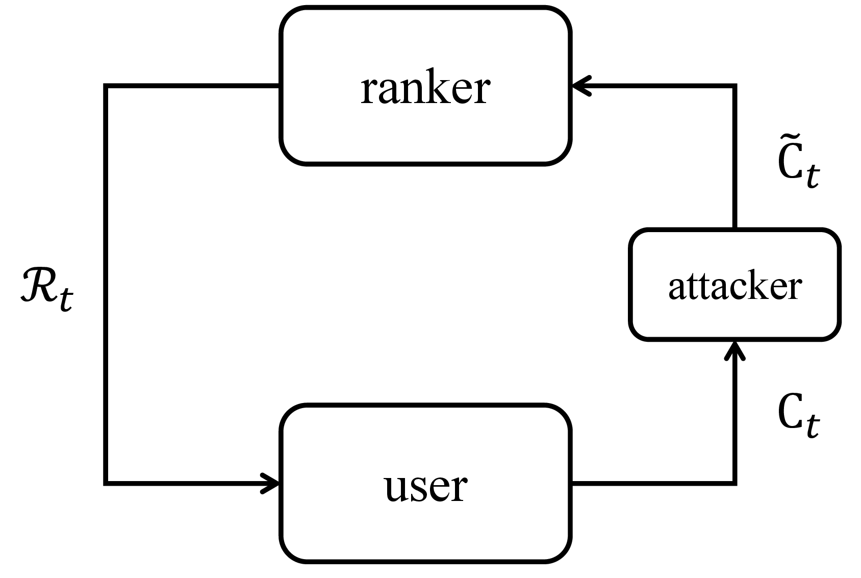
(a) Click poisoning attack.

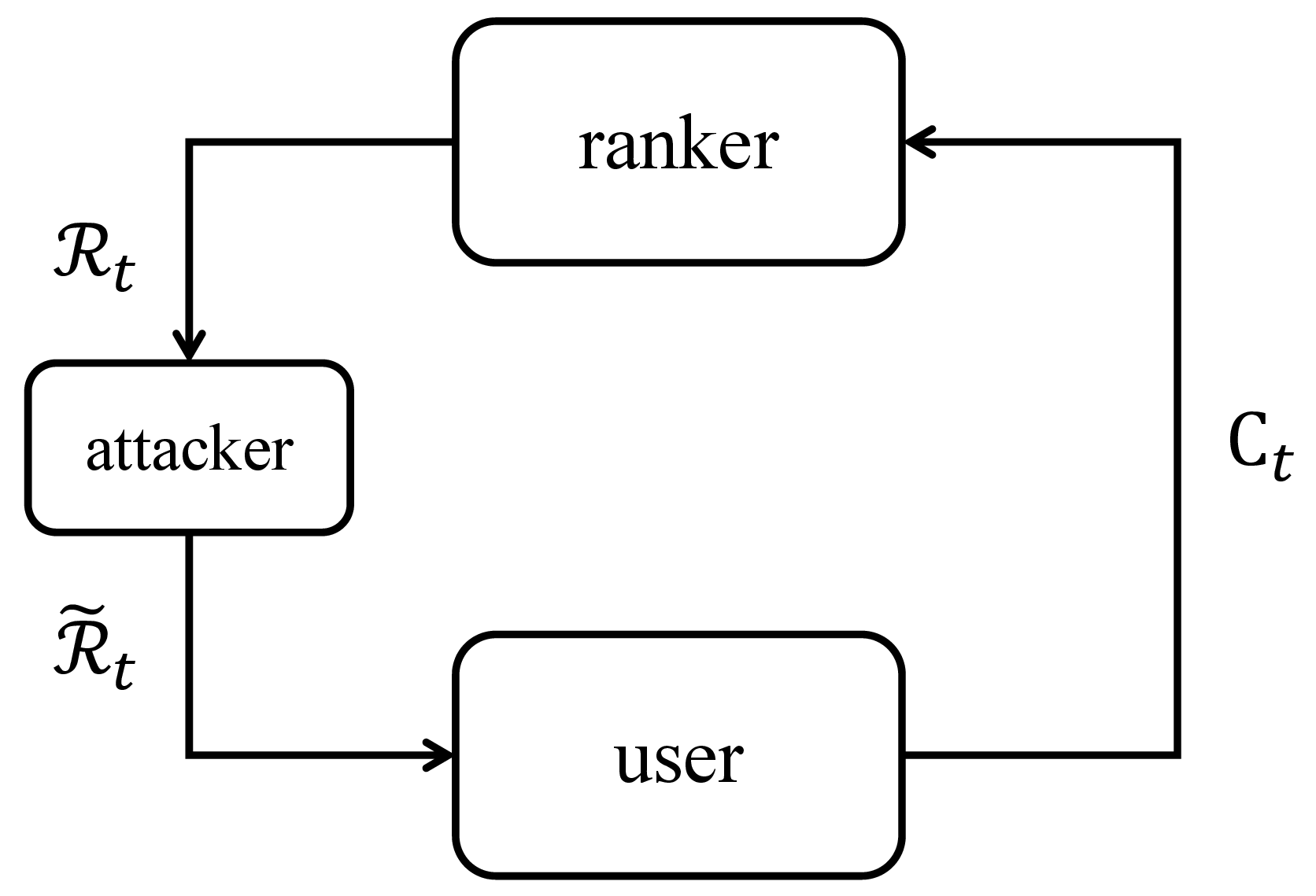
(b) List poisoning attack.

Figure 1: Threat models on online learning to rank.

Click poisoning attacks.

We illustrate click poisoning attacks in Figure 1(a). This is similar to the reward poisoning attacks studied on multi-armed bandits (Jun et al., 2018; Liu and Shroff, 2019). In each round, the attacker obtains the user’s feedback ${\mathcal{C}}_{t}$, and modifies it to perturbed clicks $\tilde{{\mathcal{C}}}_{t}=(\tilde{{\mathcal{C}}}_{1}^{t},...,\tilde{{\mathcal{C}}}_{L}^{t})$. Naturally, the attacker needs to attain its attack goal with minimum attack cost defined as $\mathcal{C}(T)=\sum_{t=1}^{T}\sum_{k=1}^{L}|\tilde{{\mathcal{C}}}_{k}^{t}-{\mathcal{C}}_{k}^{t}|$.

List poisoning attack.

Instead of directly manipulating the click feedback, the list poisoning attacks manipulate the presented ranking list from ${\mathcal{R}}_{t}$ to $\tilde{{\mathcal{R}}}_{t}$ as illustrated in Figure 1(b). This is similar to the action poisoning attack proposed by Liu and Lai (2020, 2021) against multi-armed bandits. We assume the attacker can access items with low attractiveness denoted as $\{\eta_{k}\}_{k=1}^{2K+1}\not\in\mathcal{D}$ and for convenience, $\alpha(\eta_{1})>,...,>\alpha(\eta_{2K-1})$. The low attractiveness items satisfy $\alpha(\eta_{1})<\alpha(a_{L})$. We suppose the attacker does not need to know the actual attractiveness of these items, but only their relative utilities, i.e., the attractiveness of items in $\{\eta_{k}\}_{k=1}^{K-1}$ is larger than items in $\{\eta_{k}\}_{k=K}^{2K-1}$. The attacker uploads these items to the candidate action set before exploration and we denote $\tilde{\mathcal{D}}=\mathcal{D}\cup\{\eta_{k}\}_{k=1}^{2K+1}$. In each round, the attacker can replace items in original ranking ${\mathcal{R}}_{t}$ with items in $\{\eta_{k}\}_{k=1}^{2K-1}$. This modified list $\tilde{{\mathcal{R}}}_{t}=(\tilde{\mathbb{a}}^{t}_{1},...,\tilde{\mathbb{a}}^{t}_{K})$ is then sent to the user. The cost of the attack is $\mathcal{C}(T)=\sum_{t=1}^{T}\sum_{k=1}^{K}\mathds{1}\{\tilde{\mathbb{a}}^{t}_{k}\neq{\mathbb{a}}^{t}_{k}\}$. Note that the click feedback $\mathcal{C}_{t}$ in list poisoning attacks is generated by $\tilde{\mathcal{R}}_{t}$ instead of $\mathcal{R}_{t}$, but the ranker assumes that the feedback is for $\mathcal{R}_{t}$.

In practice, the click poisoning attack could be related to fake clicks/click farms as mentioned in WSJ (2018); BuzzFeed (2019); Golrezaei et al. (2021); list poisoning attack could be achieved by malware installed as a browser extension, where the malware does not directly change the click feedback but can manipulate the web page of ranking list locally. We aim to design efficient attack strategies against online rankers, which is defined as follows.

Definition 3 (Efficient attack).

We say an attack strategy is efficient if

1. It misguides an online stochastic ranker to place the target item $\tilde{a}$ at the first position of ${\mathcal{R}}_{t}$ for $T-o(T)$ times in expectation with cost $\mathcal{C}(T)=o(T)$.

2. To keep the click poisoning attack stealthy, the returned total clicks $\sum_{k=1}^{L}\tilde{{\mathcal{C}}}_{k}^{t}$ in the cascade model is at most $1$ and in the position-based model is at most $K$.

We conclude the preliminary with the difference between poisoning attacks on stochastic bandits (Jun et al., 2018; Liu and Shroff, 2019; Xu et al., 2021) and online learning rankers. Data poisoning attack on stochastic bandits aims to fool the bandit algorithm to pull the target arm $T-o(T)$ times with $o(T)$ cost. The main idea of this class of attack strategies is to hold the expected reward of the target item and reduce the expected reward of the non-target items. However, in the OLTR setting, 1) the ranker would interact with a length $K$ list ${\mathcal{R}}_{t}$ instead of a single arm; 2) the user would generate click feedback under different click models that depend on examination probability. Recall from the definition of click models, in the position-based model the user would return at most $K$ clicks in one round, while in the cascade model, the user would return at most $1$ click. Thus, if the attacker returns more than one click in the cascade model, its attack is unstealthy and inefficient.

3 Generalized list poisoning attack strategy

In this section, we would propose a generalized list poisoning attack (GA) that misguides any no-regret ranker to place the target item at the first position of $\mathcal{R}_{t}$ for $T-o(T)$ times in expectation with $o(T)$ cost.

Algorithm 1 Generalized List Poisoning Attack (GA)

1:  Inputs: List $\mathcal{T}=(\tilde{a},\eta_{1},...,\eta_{K-1})$ and $\{\eta_{k}\}_{k=1}^{2K-1}$

2:  Upload $\{\eta_{k}\}_{k=1}^{2K-1}$ to the candidate action set

3:  for $t=1:T$ do

4:   Observe $\mathcal{R}_{t}=(\mathbb{a}_{1}^{t},...,\mathbb{a}_{K}^{t})$

5:   if $\mathcal{R}_{t}\backslash\mathcal{T}\not=\emptyset$ then

6:    for $k=1:K$ do

7:     if $\mathbb{a}_{k}^{t}\not\in\mathcal{T}$ then

8:      Set $\tilde{\mathbb{a}}_{k}^{t}=\eta_{K+k-1}$.

9:     else

10:      Set $\tilde{\mathbb{a}}_{k}^{t}=\mathbb{a}_{k}^{t}$

11:    Return $\tilde{\mathcal{R}}_{t}=(\tilde{\mathbb{a}}_{1}^{t},...,\tilde{\mathbb{a}}_{K}^{t})$ to the user

12:   else

13:    Do not attack

GA against no-regret rankers.

We briefly illustrate the process of GA. The strategy is summarized in Algorithm 1. The attacker first needs to design list $\mathcal{T}$, where $\mathcal{T}=\{\tilde{a},\eta_{1},...,\eta_{K-1}\}$. Intuitively, items $\eta_{1},...,\eta_{K-1}$ are utilized to fill in the rest of the positions when $\tilde{a}$ is in $\mathcal{R}_{t}$. The attacker would not manipulate item $\mathbb{a}_{k}^{t}\in\mathcal{T}$. If items $\mathbb{a}_{k}^{t}\in\tilde{\mathcal{D}}/\mathcal{T}$ are placed in the position $k$, the attacker would replace it with $\eta_{K+k-1}$ (lines 5-9 in Algorithm 1). This manipulation strategy can mislead the ranker to believe the items in $\tilde{D}/\mathcal{T}$ are smaller than $\alpha(\eta_{K})$ (due to $\alpha(\eta_{K})<\alpha(\eta_{K-1})<\alpha(a_{L})$). Hence, list $\mathcal{T}$ would be deemed as the optimal list and $\tilde{a}$ is the item with the highest attractiveness. Theorem 1 demonstrates that GA can efficiently attack any no-regret ranker.

Theorem 1.

GA can efficiently attack any no-regret ranker, i.e., $\mathds{E}[N_{T}(\tilde{a})]=T-o(T)$ and $\mathcal{C}(T)=o(T)$.

Although we do not include all rankers with $o(T)$ regret in the cascade model as no-regret rankers from Remark 1, we can still show that classic cascade ranking algorithms such as CascadeUCB1 (Kveton et al., 2015a) can be efficiently attacked by Algorithm 1.

Theorem 2.

Consider the ranker applies CascadeUCB1 and is attacked by Algorithm 1. The expected number of $\tilde{a}$ be placed at the first position till round $T$ satisfies

$$\begin{split}\mathds{E}[N_{T}(\tilde{a})]\geq T-\sum_{k=1}^{K-1}\frac{3+81\log(T)}{(\alpha(\tilde{a})-\alpha(\eta_{k}))^{2}}-\sum_{k=1}^{L+K-1}\frac{3+81\log(T)}{(\alpha(\tilde{a})-\alpha(\eta_{K}))^{2}}\end{split}$$ (7)

and the cost is $o(T)$.

After the above observation, one may wonder why we don’t utilize click poisoning strategy to achieve the same goal of GA, we propose an motivated example.

Example 1.

Consider an example of the Cascade model, where the examination probability of an item in $\mathcal{R}_{t}$ is related to other items’ attractiveness in $\mathcal{R}_{t}$. We suppose the case when item $a_{1}\in\mathcal{T}$ is placed before item $a_{2}\not\in\mathcal{T}$ and the click feedback of item $a_{1}$ is $1$ (which implies the user will not examine the following items and thus true click feedback of $a_{2}$ will be $0$). If the attacker trivially reduces the click feedback of all the items $\not\in\mathcal{T}$ to $0$ (which is a common strategy of attack on bandits (Jun et al., 2018; Garcelon et al., 2020)), this can be interpreted as the attractiveness of item $a_{2}$ is reduced to $0$. Since $a_{1}$ is not clicked, the following items should be examined and the OLTR algorithm would recognize items placed after $a_{1}$ (includes $a_{2}$) as $0$ attractiveness. The click manipulation strategy clearly harms the attack in this cascade model example, making the attack results hard to be analyzed. According to this instance, existing reward (e.g., click) poisoning strategies on bandits can hard to be proved to succeed in different click models, as the clicks should be manipulated according to the property of the click model. However, our GA can adapt to stochastic click models for any no-regret ranker and enjoys a simple theoretical characteristic.

Remark 2.

The idea of GA against online stochastic rankers is similar to the previous reward poisoning attack idea against stochastic bandits, i.e., reduces the expected reward (i.e., clicks) of the non-target items and holds the expected reward of the target item. The main difference is 1) we enlarge our target from an item to a list; 2) we manipulate the ranking list $\mathcal{R}_{t}$ instead of manipulating ’rewards’; 3) the attack is applied to the comprehensive stochastic click models.

4 Attack-then-quit strategy

In this section, we provide a click poisoning attack strategy that applied to elimination-based rankers and divide-and-conquer-based rankers. We will demonstrate our strategy can efficiently attack some specific rankers under any click models. Previous reward poisoning attack strategies on multi-armed bandits only manipulate the reward of the non-target item and never perturb the reward of the target item (Jun et al., 2018; Liu and Shroff, 2019; Garcelon et al., 2020; Wang et al., 2022). However, the attack strategy proposed in this section perturbs the click feedback of every item. The attacker would spend a linear cost in a short period $T_{1}=o(T)$ and then stop the attack and quit. Thus, we call our attack strategy the attack-then-quit (ATQ) strategy.

As mentioned in the previous section, the BatchRank and TopRank can work in general stochastic click models, while other UCB-type algorithms can only work in specific click models (e.g., CascadeUCB1 or PBM-UCB). Hence, the BatchRank and TopRank can be deemed as the superior ranker to those UCB-type algorithms, which are worth more significant consideration. Moreover, to our best knowledge, current algorithms dedicate to the stochastic click models all follow the elimination/divide-and-conquer idea.

4.1 Click poisoning-based ATQ

Algorithm 2 can efficiently attack elimination-based rankers (e.g., BatchRank) and divide-and-conquer-based rankers (e.g., TopRank). At the initialization stage, the attacker would receive target item $\tilde{a}$ and threshold $T_{1}$. In each round, if click feedback $\mathcal{C}_{k}^{t}$ is returned from $\tilde{a}$ and $\tilde{a}\in\mathcal{R}_{t}$, the attacker would set $\tilde{\mathcal{C}}_{k}^{t}=1$, otherwise, $\tilde{\mathcal{C}}_{k}^{t}=0$. Besides, as we mention in Assumption 1 and Definition 1, the item $a_{k}\not\in\mathcal{R}_{t}$ would not be observed by the user in round $t$, and would not be clicked either. This implies their click feedback would be 0. In ATQ, the attacker does not (cannot) modify the click feedback of items $a_{k}\not\in\mathcal{R}_{t}$ (line 9$\sim$10 in Algorithm 2). After scanning $\mathcal{C}_{t}$, the attacker would return $\tilde{\mathcal{C}}_{t}=(\tilde{\mathcal{C}}_{1}^{t},...,\tilde{\mathcal{C}}_{L}^{t})$ to the ranker. Note that $\sum_{k=1}^{L}\tilde{\mathcal{C}}_{k}^{t}\leq 1$ (line 4-10 in Algorithm 2), hence Algorithm 2 can work stealthily and efficiently in different click models. Note that the general stochastic click models in (Zoghi et al., 2017) and (Lattimore et al., 2018) directly ensure $\mathcal{R}^{*}$ can uniquely maximize the expected click number. Hence, the target of BatchRank and TopRank is to quickly estimate the attractiveness of items and rank them accordingly. Our attack Algorithm 2 aims to mislead these rankers to ’believe’ the target item is the best item with the smallest rounds. Once these rankers make this judgment, they would place the target item at the first position until $T$. In the following sections, we will demonstrate Algorithm 2 can efficiently attack BatchRank and TopRank with suitable $T_{1}$.

Algorithm 2 Attack-Then-Quit (ATQ) Algorithm

1:  Inputs: The target item $\tilde{a}$, threshold $T_{1}$

2:  for $t=1:T_{1}$ do

3:   Observe $\mathcal{C}_{t}=(\mathcal{C}_{1}^{t},...,\mathcal{C}_{L}^{t})$ and $\mathcal{R}_{t}=(\mathbb{a}_{1}^{t},...,\mathbb{a}_{K}^{t})$

4:   for $k=1:L$ do

5:    if $a_{k}=\tilde{a}$ and $a_{k}\in\mathcal{R}_{t}$ then

6:     Set $\tilde{\mathcal{C}}_{k}^{t}=1$

7:    else if $a_{k}\not=\tilde{a}$ and $a_{k}\in\mathcal{R}_{t}$ then

8:     Set $\tilde{\mathcal{C}}_{k}^{t}=0$

9:    else

10:     Set $\tilde{\mathcal{C}}_{k}^{t}=\mathcal{C}_{k}^{t}$

11:   Return $\tilde{\mathcal{C}}_{t}=(\tilde{\mathcal{C}}_{1}^{t},...,\tilde{\mathcal{C}}_{L}^{t})$ to the ranker

4.2 Attack on BatchRank

Brief explanation of BatchRank.

The BatchRank falls into the category of elimination-based algorithms (Zoghi et al., 2017). The BatchRank would begin with stage $\ell_{1}=0$ and the first batch $B_{1,\ell_{1}}=\mathcal{D}$. In stage $\ell_{1}$, every item would be explored for $\displaystyle{\bm{n}}_{\ell_{1}}=16\tilde{\Delta}^{-1}_{\ell_{1}}\log(T)$ times and $\tilde{\Delta}^{-1}_{\ell_{1}}=2^{-\ell_{1}}$. Afterward, if BatchRank collects enough information to confirm the attractiveness of every item in a group is larger than the others, BatchRank then splits the initial batch into two sub-batches $B_{2,\ell_{2}}$ and $B_{3,\ell_{3}}$. Items that are considered with higher attractiveness (i.e., in sub-batch $B_{2,\ell_{2}}$) would be always placed before items with lower attractiveness (i.e., in sub-batch $B_{3,\ell_{3}}$). The BatchRank would restart with stage $\ell_{2}=0$ and $\ell_{3}=0$ and sub-batches $B_{2,\ell_{2}}$ and $B_{3,\ell_{3}}$. Batches would recursively split until round $T$. Intuitively, the action ‘split’ of BatchRank is similar to the elimination action in the elimination-based bandit algorithms (Even-Dar et al., 2006; Lykouris et al., 2018; Bogunovic et al., 2021). The details of BatchRank are provided in the appendix.

Algorithm 2 can successfully attack BatchRank owing to BatchRank’s elimination property. Algorithm 2 maximizes the returned clicks of the target item and minimizes the returned click of the non-target item in a short period $o(T)$. After this period, BatchRank regards the target item owning the highest attractiveness (i.e., split). Then the target item would be always placed at the first position of the list $\mathcal{R}_{t}$ and the attacker achieves the attack goal. We also provide an example in the appendix to further illustrate the process of Algorithm 2 attack BatchRank.

Theorem 3 (Attack against BatchRank).

Consider the attacker aims to attack BatchRank with stochastic click models (Zoghi et al., 2017). If the attacker runs Algorithm 2 with $T_{1}=16L\log(T)$, we have $N_{T}(\tilde{a})\geq T-T_{1}$ and the cost can be bounded by $\mathcal{C}(T)\leq KT_{1}$.

Besides BatchRank, this attack idea can also be utilized to attack some rankers that do not belong to the elimination-based category, such as TopRank.

4.3 Attack on TopRank

Brief explanation of TopRank.

TopRank is a divide-and-conquer-based ranker (Lattimore et al., 2018). It begins with a blank graph $G_{1}=\emptyset$. In round $t$, TopRank would establish blocks $\mathcal{P}_{t1},...,\mathcal{P}_{td}$ via graph $G_{t}$. The items in block $\mathcal{P}_{t1}$ would be placed at the first $|\mathcal{P}_{t1}|$ positions and the items in block $\mathcal{P}_{t2}$ would be placed at the next $|\mathcal{P}_{t2}|$ positions, and so on. During rounds $1$ to $T$, TopRank would explore items with blocks, collect click information and compare attractiveness between items in the same block. If the collected evidence is enough to let TopRank regards the attractiveness of item $a_{i}$ as larger than the attractiveness of item $a_{j}$, a directional edge $(a_{j},a_{i})$ would be established. This behavior is similar to the ‘split’ action in BatchRank. Besides, graph $G_{t}$ would not contain cycles with high probability. If the graph contains at least one cycle, we consider TopRank would be out of control. Details of TopRank are provided in the appendix.

Note that if there exist edges from every non-target item to the target item and $G_{t}$ contains no cycle, then the target item would be isolated from the non-target items and would always be placed at the first position of $\mathcal{R}_{t}$. This is because the first block only contains the target item. We also provide an example to specifically explain how Algorithm 2 attacks TopRank in the appendix.

Theorem 4 (Attack against TopRank).

Consider the attacker aims to attack TopRank and TopRank runs in the click model in (Lattimore et al., 2018). If the attacker sets $T_{1}=\frac{4\log(c/\delta)}{\frac{K}{L}+(1-\sqrt{1+8K/L})/4}$ and runs Algorithm 2. The attacker can achieve $N_{T}(\tilde{a})\geq T-T_{1}$ with probability at least $1-(1/c+L^{2})\delta$. The cost can be bounded by $\mathcal{C}(T)\leq KT_{1}$.

By choosing $\delta=1/T$ and $c=4\sqrt{2/\pi}/\emph{erf}(\sqrt{2})\approx 3.43$ which is same as in TopRank algorithm, we have $T_{1}=O((L/K)\log T)$. The proof of Theorem 4 mainly focuses on how to bound the number of the target item to be placed in $\mathcal{R}_{t}$ ($\sum_{s=1}^{t}\mathds{1}\{\tilde{a}\in\mathcal{R}_{s}\}$) when $G_{t}=\emptyset$. Note that we can manipulate the click of the target item only if $\tilde{a}\in\mathcal{R}_{t}$. Hence, we can deduce when are the edges from the non-target item to the target item established with $\sum_{s=1}^{t}\mathds{1}\{\tilde{a}\in\mathcal{R}_{s}\}$. The probability of the attack failure is at most $L^{2}\delta+\delta/c$, where $L^{2}\delta$ is the intrinsic probability of TopRank’s $G_{t}$ contains cycle and $\delta/c$ is the probability the attacker fails to bound $\sum_{s=1}^{t}\mathds{1}\{\tilde{a}\in\mathcal{R}_{s}\}$ when $G_{t}(\tilde{a})=\emptyset$.

5 Experiments

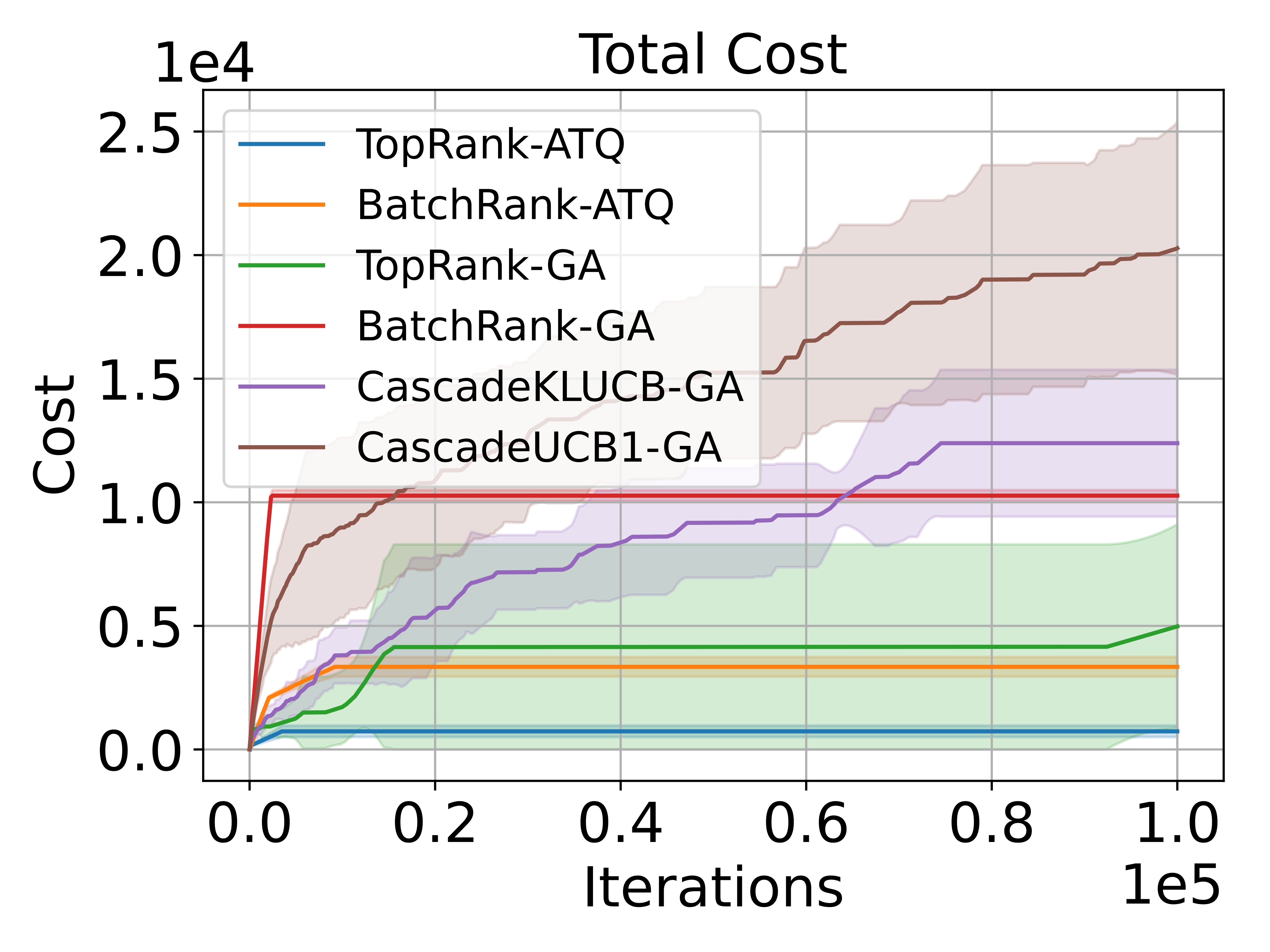
(a) Cost in CM.

(b) $N_{t}(\tilde{a})$ in CM.

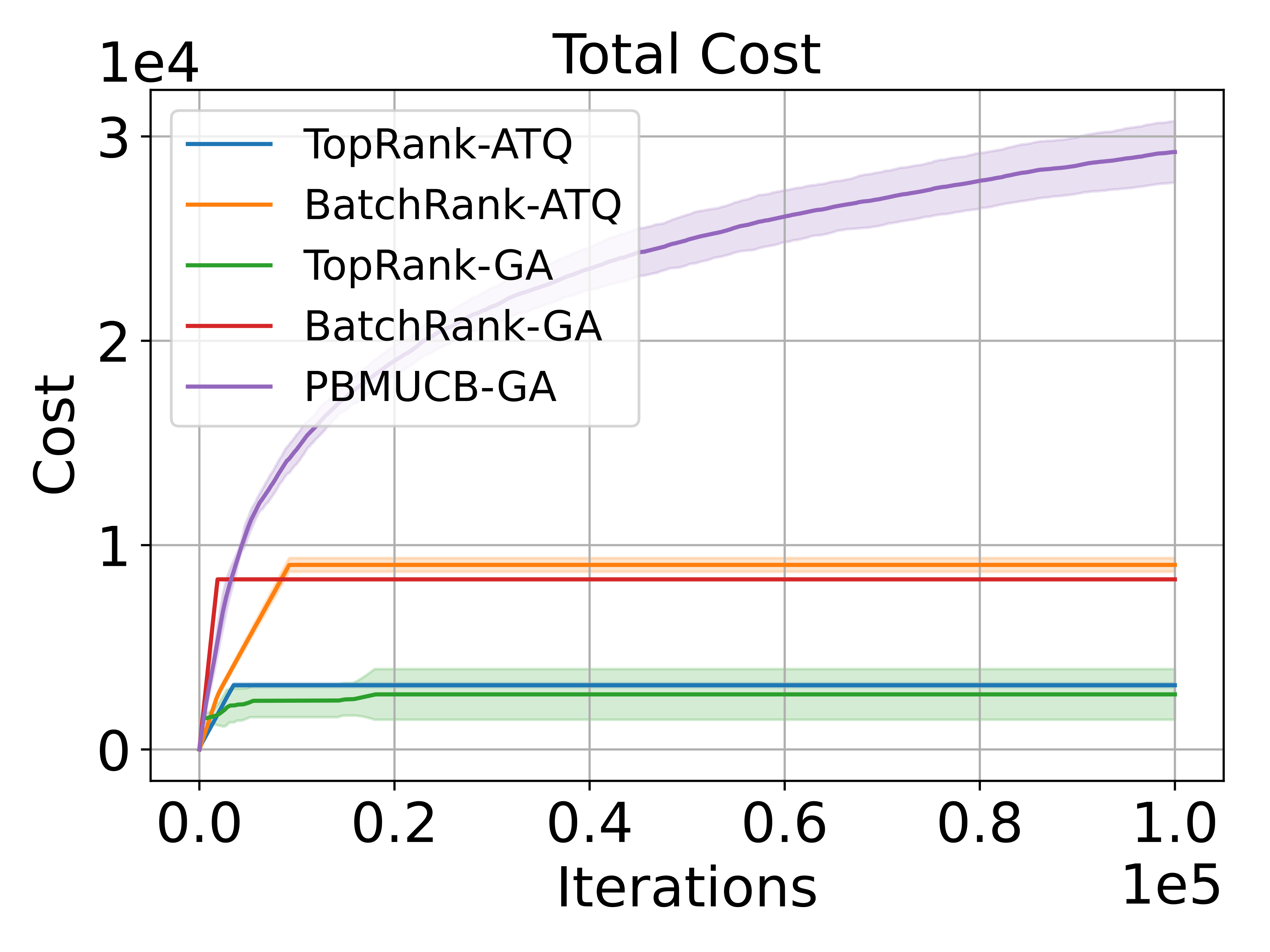
(c) Cost in PBM.

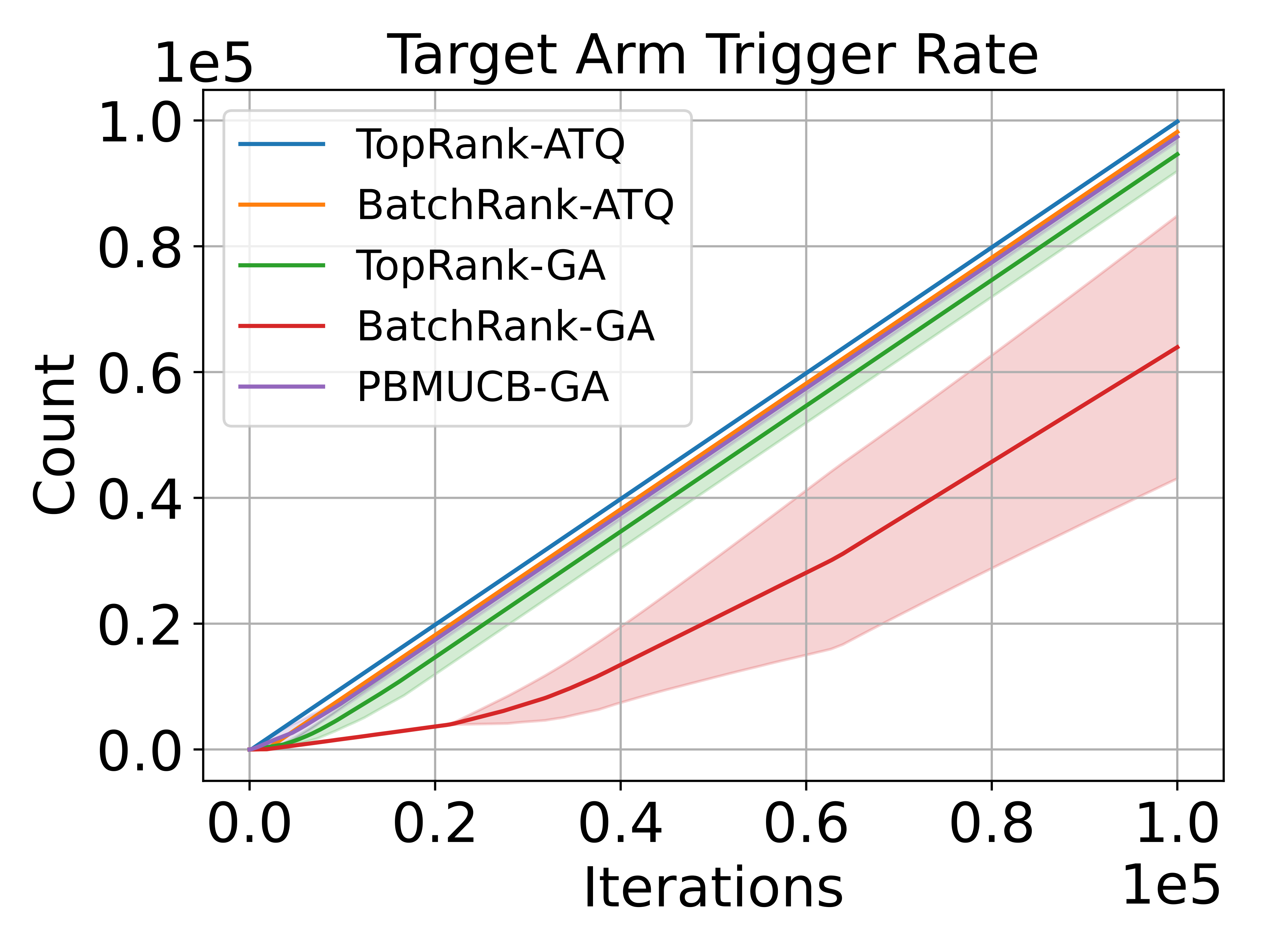
(d) $N_{t}(\tilde{a})$ in PBM.

Figure 2: Synthetic data experiment: (a) total cost spend in the cascade model, (b) $N_{t}(\tilde{a})$ in the cascade model, (c) the total cost spend in the cascade model and (d) $N_{t}(\tilde{a})$ in the position-based model. We report averaged result and variance of 10 runs.

In the experiment section, we apply the proposed attack methods against the OLTR algorithms listed in Table 1 with their corresponding click models. We compare the effectiveness of our attack on synthetic data and real-world MovieLens dataset. For all our experiments, we use $L=50$, $K=5$ (the set up of Zoghi et al. (2017); Lattimore et al. (2018) is $L=10$ and $K=5$) and $T=10^{5}$. For ATQ, we set the $T_{1}$ in Algorithm 2 by Theorem 3 and Theorem 4.

Table 1: Target ranking algorithms and their applied click models

Algorithm	Click model
BatchRank Zoghi et al. (2017)	Stochastic click model
TopRank Lattimore et al. (2018)	Stochastic click model
PBM-UCB Lagrée et al. (2016)	Position-based model
CascadeUCB1 Kveton et al. (2015a)	Cascade model
CascadeKLUCB Kveton et al. (2015a)	Cascade model

5.1 Synthetic data

First, we verify the effectiveness of our proposed attack strategies on synthetic data. We generate a size-$L$ item set $\mathcal{D}$, in which each item $a_{k}$ is related to a unique attractiveness score $\alpha(a_{k})$. Each attractiveness score $\alpha(a_{k})$ is drawn from a uniform distribution $U(0,1)$. We randomly select a suboptimal target item $\tilde{a}$. Figure 2 shows the results and variances of 10 runs.

In Figures 2(a) and 2(b), we plot the results of the GA against CascadeUCB1, CascadeKLUCB, BatchRank, and TopRank, and the ATQ against BatchRank and TopRank in the cascade model. Both attack strategies can efficiently misguide the rankers to place the target item at the first position for $T-o(T)$ times as shown in Figure 2(b), and the cost of the attack is sublinear as shown in Figure 2(a). The GA is cost-efficient when attacking all four algorithms. We can observe that when it attacks TopRank and BatchRank, the cost would not increase after some periods (similar to the ATQ’s results). This is when the TopRank and BatchRank believe the target item and the auxiliary items have a relatively higher attractiveness than the other items, they would only put the target item and the auxiliary items in $\mathcal{R}_{t}$. Besides, when attacking TopRank and BatchRank, the growth rate of GA’s target arm pulls $N_{t}(\tilde{a})$ slowly increased from $0.2$ per iteration to 1 per iteration. This is because the GA does not manipulate the items in $\mathcal{T}$ and the TopRank and BatchRank need time to confirm the target item has a higher attractiveness than $\{\eta_{k}\}_{k=1}^{K-1}$. Hence, the smaller the gap between $\tilde{a}$ and $\eta_{1}$, the larger the confirmed time. Compare with the GA, the ATQ can also efficiently attack BatchRank and TopRank with a sublinear cost. However, its $N_{T}(\tilde{a})$ is almost $T$, which is relatively larger than GA’s $N_{T}(\tilde{a})$. This is because the ATQ is specifically designed for divide-and-conquer-based algorithms like TopRank and BatchRank. The ATQ can maximize the target item’s click number and misguide these algorithms to believe the target item is the best in the shortest period.

Figures 2(c) and 2(d) report the results in the position-based model. We can observe that the spending cost of the GA on the PBM-UCB is slightly larger than the spending cost on the CascadeKLUCB and CascadeUCB1. Besides, although the GA can let the TopRank believe the target item is the best item in almost 500 iterations, it still needs a large number of iterations (around $6\times 10^{4}$ iterations) to make the BatchRank make such a decision. From the results of the two models, the ATQ is obviously more effective than the GA when the target algorithms are TopRank and BatchRank.

Due to the page limitation, the experiment results based on real-world data are provided in the appendix.

6 Related Work

Online learning to rank.

OLTR is first studied as ranked bandits (Radlinski et al., 2008; Slivkins et al., 2013), where each position in the list is modeled as an individual multi-armed bandits problem (Auer et al., 2002). Such a problem can be settled down by bandit algorithms which can maximize the expected click number in each round. Recently studied of OLTR focused on different click models (Craswell et al., 2008; Chuklin et al., 2015), including the cascade model (Kveton et al., 2015a, b; Zong et al., 2016; Li et al., 2016; Vial et al., 2022), the position-based model (Lagrée et al., 2016) and the dependent click model (Katariya et al., 2016; Liu et al., 2018). OLTR with general stochastic click models is studied in (Zoghi et al., 2017; Lattimore et al., 2018; Li et al., 2018, 2019; Gauthier et al., 2022).

Adversarial attack against bandits.

Adversarial reward poisoning attacks against multi-armed bandits have been recently studied in stochastic bandits (Jun et al., 2018; Liu and Shroff, 2019; Xu et al., 2021) and linear bandits (Wang et al., 2022; Garcelon et al., 2020). These works share a similar attack idea, where the attacker holds the reward of the target arm, meanwhile lowers the reward of the non-target arm. Besides reward poisoning attacks, other threat models such as action poisoning attacks (Liu and Lai, 2020, 2021) were also being studied. However, adversarial attack on online ranking problem has not been explored yet. In this paper, we first time studied click poisoning attacks and list poisoning attacks against OLTR algorithms. Our click poisoning attacks share the same threat model as reward poisoning attacks, and list poisoning attacks follow a similar idea as action poisoning attacks against multi-armed bandits.

7 Conclusion

In this paper, we proposed the first study of adversarial attacks on online learning to rank. Different from the poisoning attacks studied in the multi-armed bandits setting where reward or action is manipulated, the attacker manipulates binary click feedback instead of reward and item list instead of a single action in our model. In addition, due to the interference of the click models, it is difficult for the attacker to precisely control the ranker behavior under different unknown click models with simple click manipulation. Based on this insight, we developed the GA that can efficiently attack any no-regret ranking algorithm. Moreover, we also proposed the ATQ that follows the click poisoning idea, which can efficiently attack BatchRank and TopRank. Finally, we presented experimental results based on synthetic data and real-world data that validated the cost-efficient and effectiveness of our attack strategies.

In our future work, it is interesting to study the adversarial attack on online learning to rank where the target is a list instead of a single item. Another intriguing direction is to establish robust rankers against poisoning attacks. In the ideal case, the robust ranker should achieve sublinear regret in general stochastic click models under different threat models.

Appendix A Notations

For clarity, we collect the frequently used notations in this paper.

$\mathcal{D}$	Total item set
$\mathcal{R}_{t}$	$K$-length item list be shown to the user in round $t$
$\mathcal{R}^{*}$	Optimal list
$\tilde{\mathcal{R}}_{t}$	Manipulated list in round $t$
$\mathcal{C}_{t}$	Click feedback list in round $t$
$\tilde{\mathcal{C}}_{t}$	Manipulated click feedback list in round $t$
$\mathcal{T}$	Ordered list $(\tilde{a},\bar{a}_{1},...,\bar{a}_{K})$
$\tilde{a}$	Target item
$a_{k}$	$k$-th most attractive item in $\mathcal{D}$
$\bar{a}_{k}$	$k$-th most attractive auxiliary item
$\eta_{k}$	Particular item in the list poisoning attack
$\alpha(a_{k})$	Attractiveness of item $a_{k}$
$\mathbb{a}_{k}^{t}$	Item on the $k$-th position in $\mathcal{R}_{t}$
$\tilde{\mathbb{a}}_{k}^{t}$	Manipulated item on the $k$-th position in $\tilde{\mathcal{R}}_{t}$
$\mathcal{C}_{k}^{t}$	Click feedback of item $a_{k}$ in round $t$
$\tilde{\mathcal{C}}_{k}^{t}$	Manipulated click feedback of the item $a_{k}$ in round $t$
$v(\mathcal{R}_{t},\mathbb{a}_{k}^{t},k)$	Click probability of item at the $k$-th position in round $t$
$R(T)$	Cumulative regret in $T$ rounds
$\mathcal{C}(T)$	Total cost in $T$ rounds
$N_{t}(a_{k})$	Number of item $a_{k}$ be placed at the first position in $t$ rounds
$\mathcal{N}_{t}(a_{k})$	Number of item $a_{k}$ be examined in $t$ rounds
$T$	Total number of interaction
$T_{1}$	Input threshold value of the attack-then-quit algorithm
BatchRank
$b$	Batch index
$\ell$	Stage index
$B_{b,\ell}$	$b$-th batch explored in stage $\ell$
$\displaystyle{\bm{n}}_{\ell}$	Exploration number of item in batch $B_{b,\ell}$ in stage $\ell$
$\mathcal{C}_{b,\ell}(a_{k})$	Total received click number of item $a_{k}$ during stage $\ell$
$\hat{\mathcal{C}}_{b,\ell}(a_{k})$	Attractiveness estimator of item $a_{k}$ in stage $\ell$
$U_{b,\ell}(a_{k})$	Upper confidence bound of item $a_{k}$ in stage $\ell$
$L_{b,\ell}(a_{k})$	Lower confidence bound of item $a_{k}$ in stage $\ell$
TopRank
$G_{t}$	Auxiliary graph in round $t$
$(a_{j},a_{i})$	Directional edge from item $a_{j}$ to item $a_{i}$
$\mathcal{P}_{tc}$	$c$-th block in round $t$
$S_{tij}$	Sum of the $U_{tij}$ from round $1$ to $t$
$N_{tij}$	Sum of the absolute value of $U_{tij}$ from round $1$ to $t$

Appendix B Additional experiment

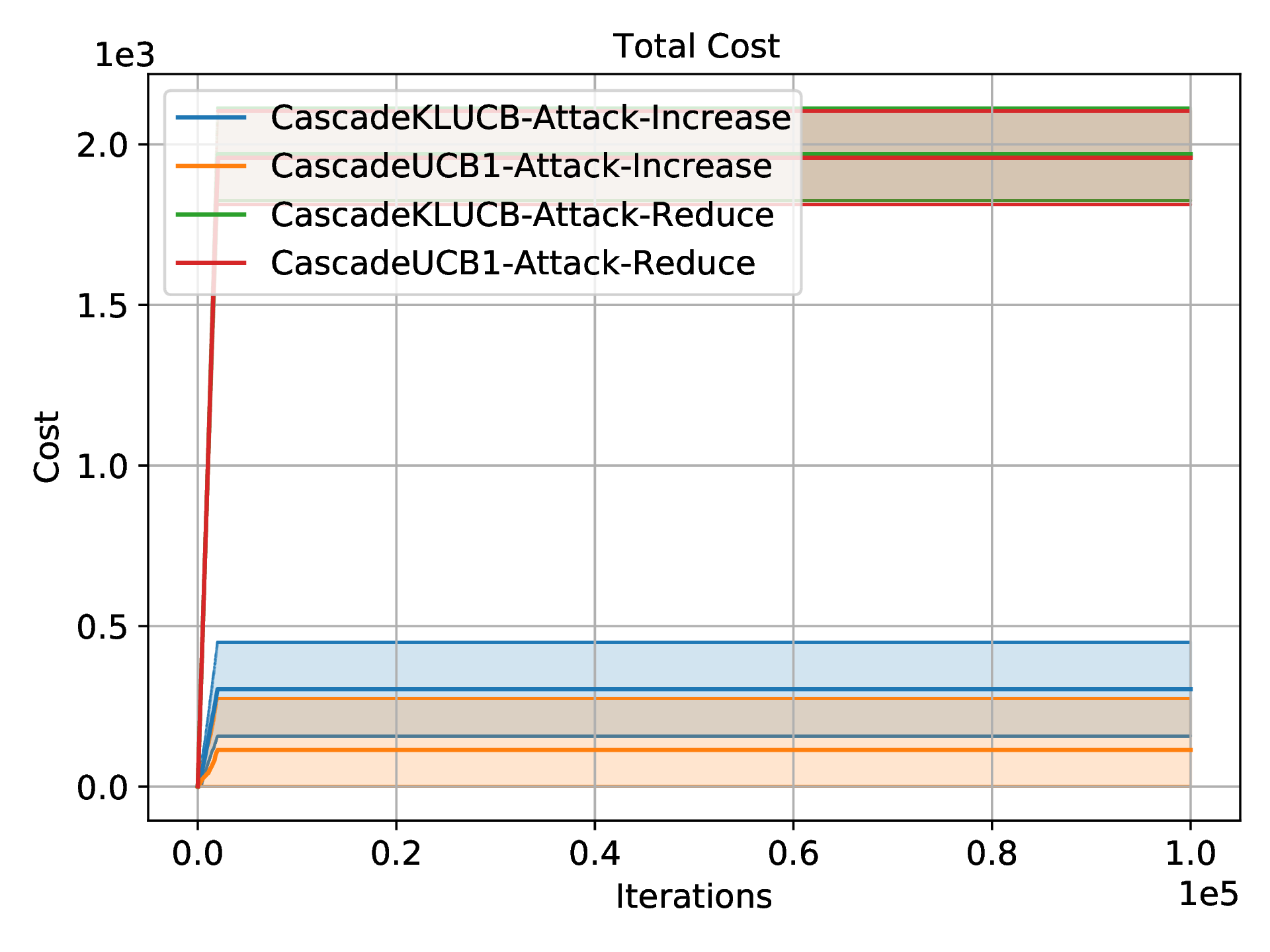
(a) Cost in CM.

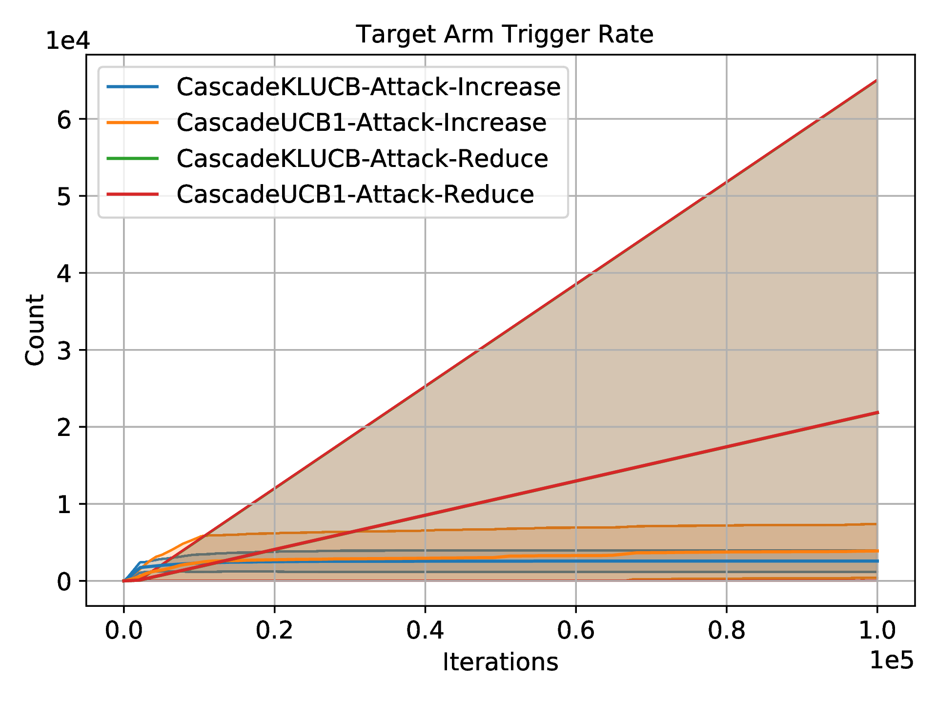
(b) $N_{t}(\tilde{a})$ in CM.

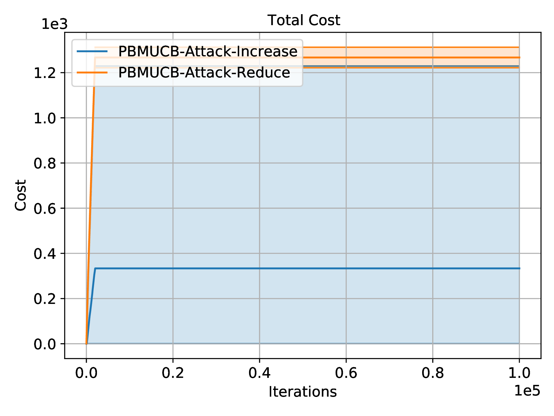
(c) Cost in PBM.

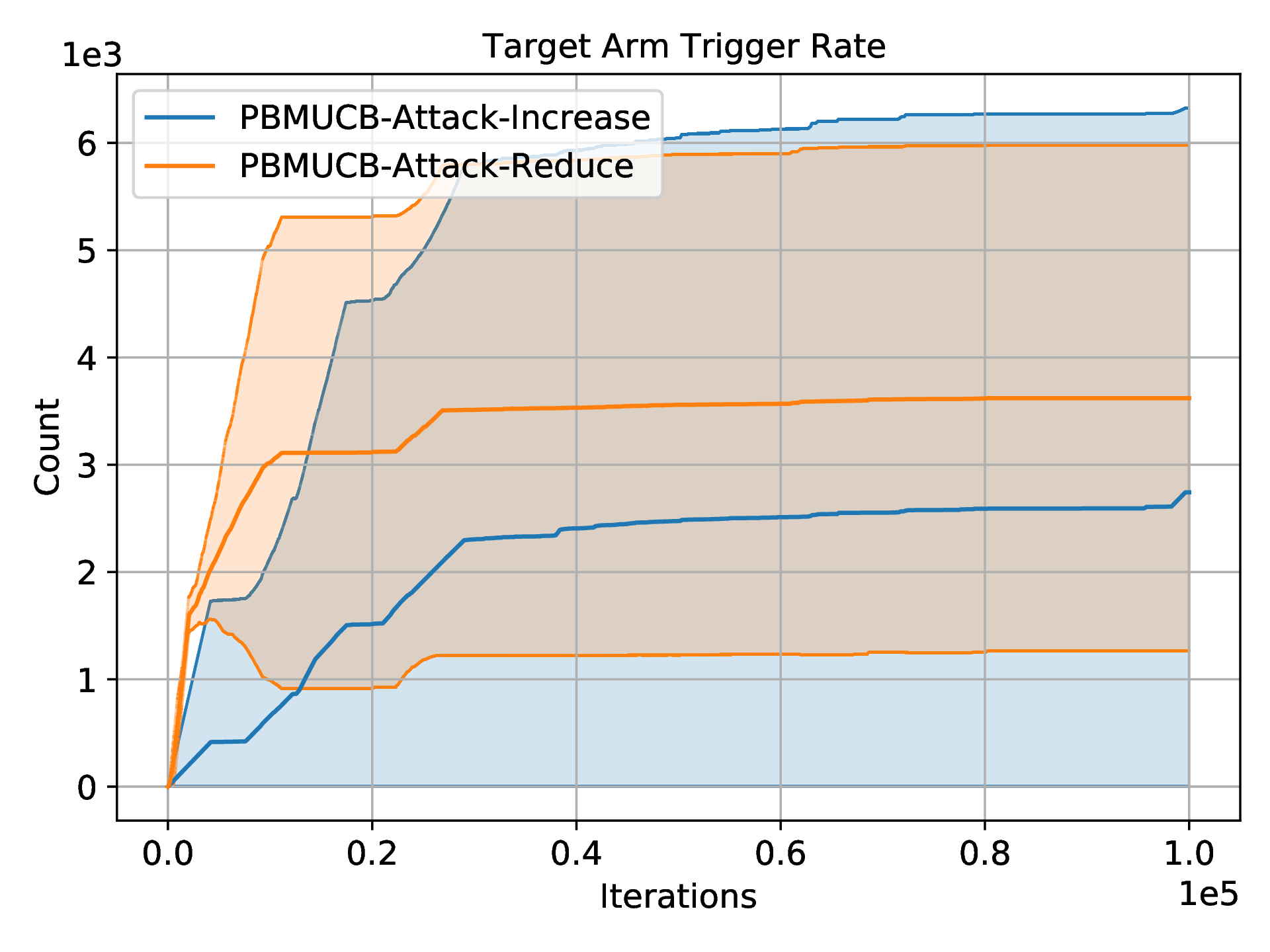
(d) $N_{t}(\tilde{a})$ in PBM.

Figure 3: Additional baseline: (a) the total cost spend in the cascade model, (b) $N_{t}(\tilde{a})$ in the cascade model, (c) the total cost spend in the cascade model and (d) $N_{t}(\tilde{a})$ in the position-based model. We report averaged result and variance of 10 runs.

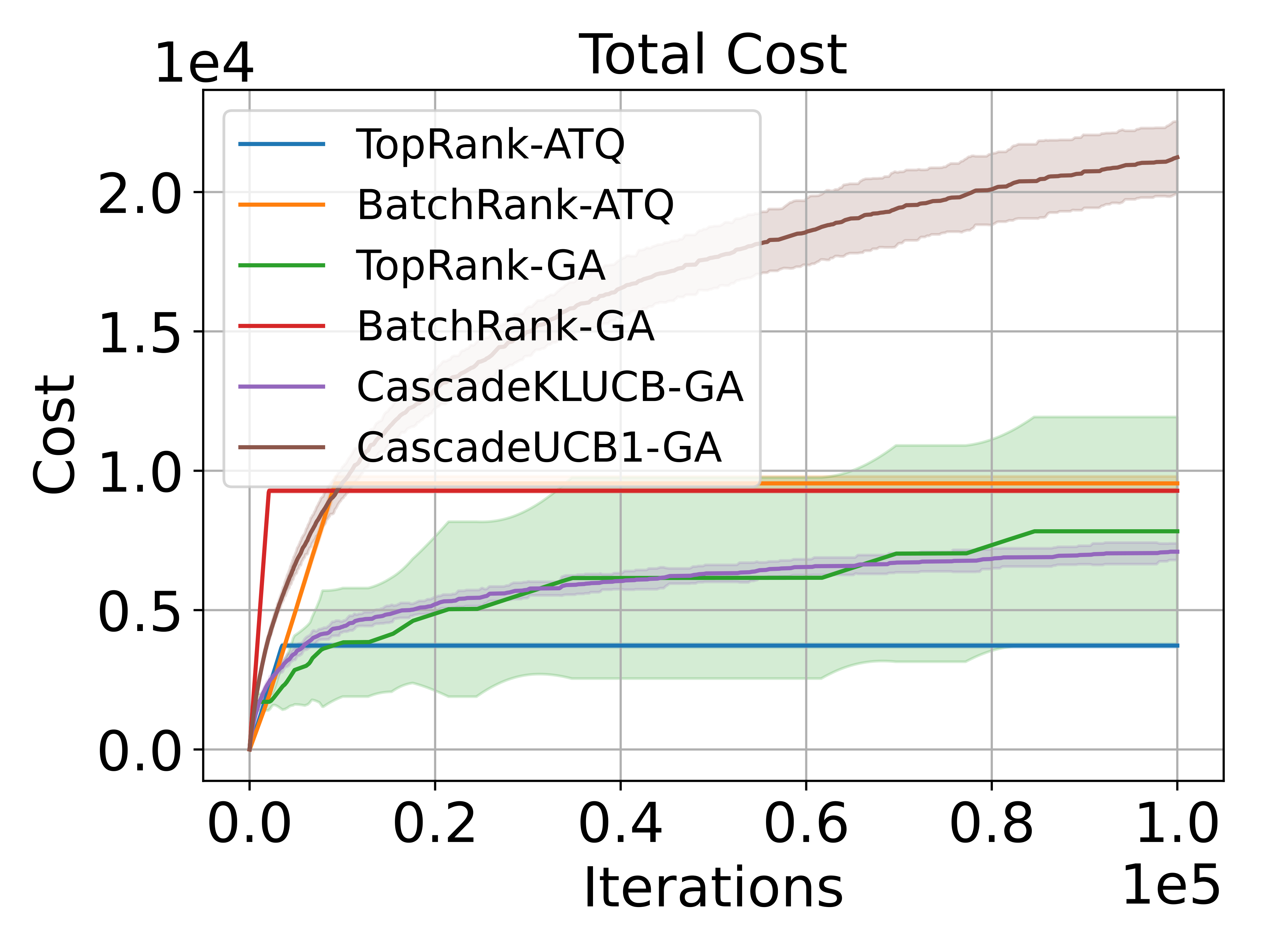
(a) Cost in CM.

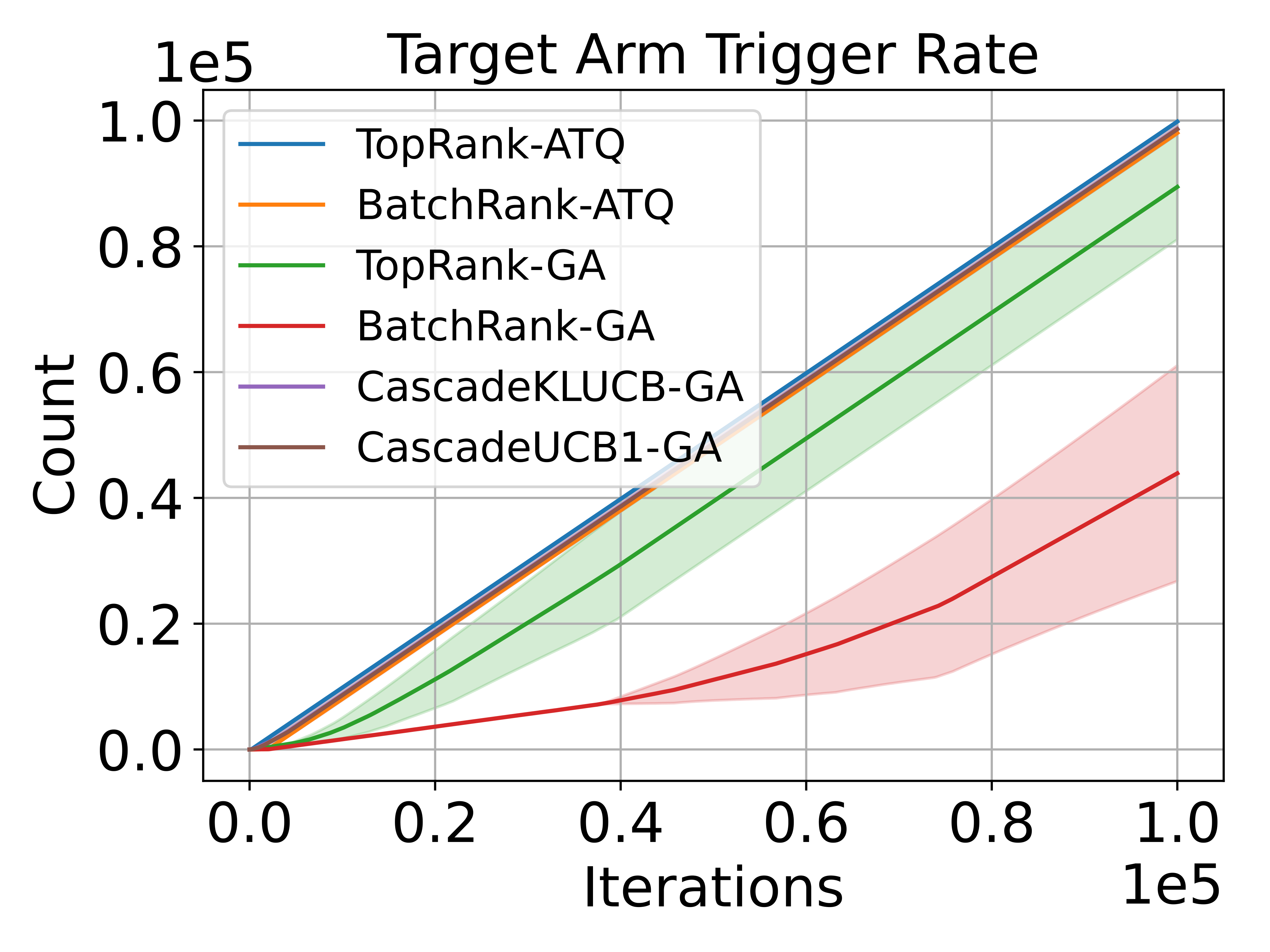
(b) $N_{t}(\tilde{a})$ in CM.

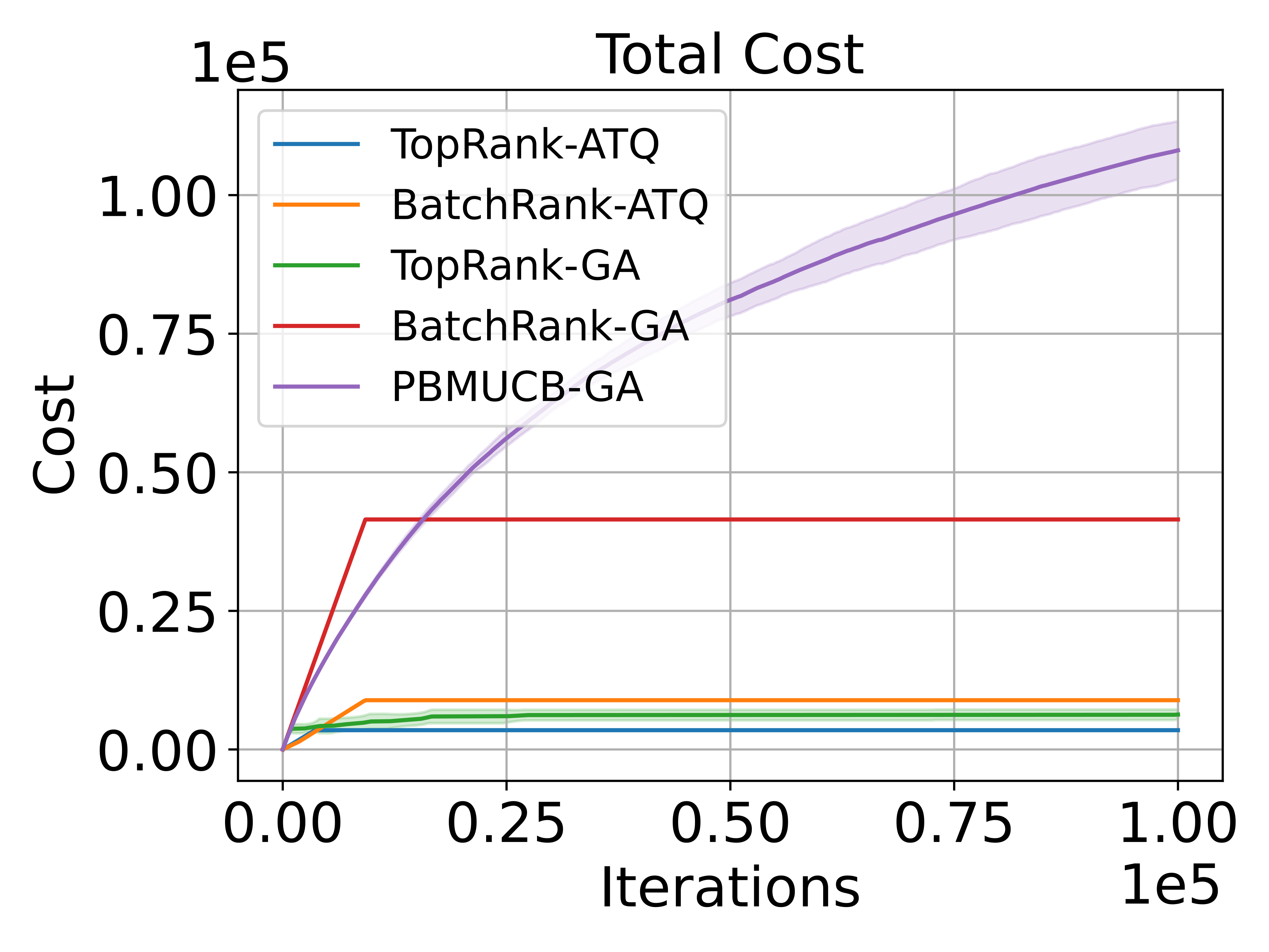
(c) Cost in PBM.

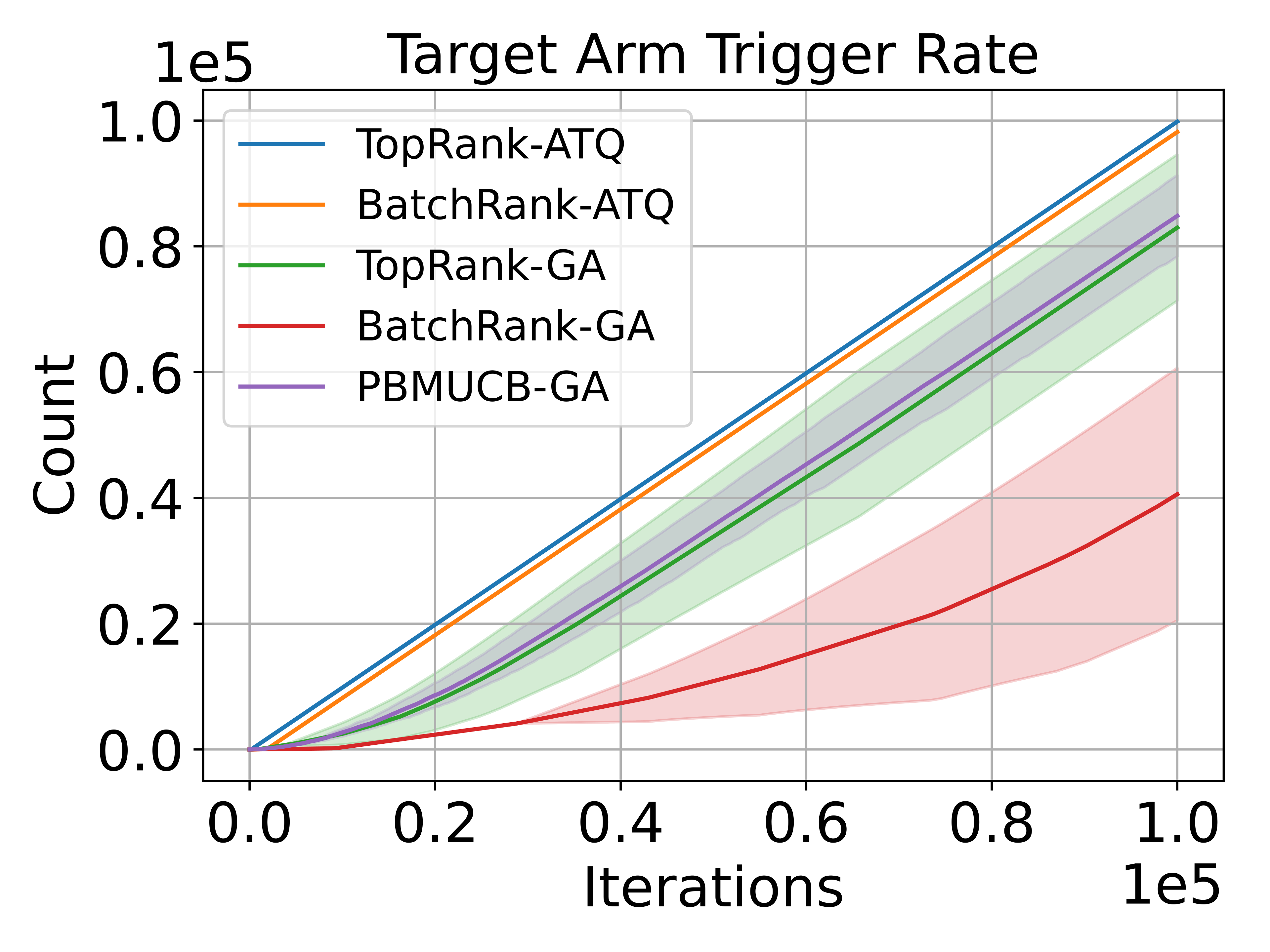
(d) $N_{t}(\tilde{a})$ in PBM.

Figure 4: MovieLens experiment: (a) the total cost spend in the cascade model, (b) $N_{t}(\tilde{a})$ in the cascade model, (c) the total cost spend in the cascade model and (d) $N_{t}(\tilde{a})$ in the position-based model. We report averaged result and variance of 10 runs.

B.1 Additional experiments on synthetic data

Since we propose the first attack against OLTR, there are no existing baseline attack strategies in the literature to compare with. Nevertheless, We build two additional simple click-poisoning attack strategies as baselines. The setting of this experiment is the same as our experiment on synthetic data in Section 5. The first baseline directly reduces all the non-target item’s click feedback to $0$ in the first two thousand rounds (indexed by Attack-reduce). The second baseline directly increases the click feedback of the target item to $1$ when the target item is in $\mathcal{R}_{t}$ in the first two thousand rounds. These two attack strategies are tested to attack OLTR algorithms CascadeUCB1, KL-CascadeUCB, and PBM-UCB. The attack results are provided in Figure 3.

From Figure 3, we can observe that although baseline attacks achieve a sublinear cost (due to their stopping attack at around $2000$), none of them can fool at least one of the target algorithms to place the target item at the top position for $T-o(T)$ times. However, our attack strategies (including GA and ATQ) can efficiently attack all of these target OLTR algorithms, which are shown in Section 5.

B.2 Experiments on real-world data

We also evaluate the proposed attacks on MovieLens dataset (Harper and Konstan, 2016). We first split the dataset into train and test data subsets. Using the training data, we compute a $d$-rank SVD approximation, which is used to compute a mapping from movie rating to the probability that a user selected at random would rate the movie with 3 stars or above. We use the learned probability to simulate user’s clicks given the ranking list. We refer the reader to the Appendix C of (Vial et al., 2022) for further details. Figure 4 shows the attack results of our attack strategy averaged over $10$ rounds.

We can observe that the trends in Figure 4 are similar to those in Figure 2, and the two attack algorithms are again able to efficiently fool the OLTR algorithms. In the cascade model, we see that successfully attacking CascadeKLUCB, TopRank, and BatchRank with GA only needs a relatively low cost, and the cost is higher when the target is CascadeUCB1. Besides, the ATQ strategy can still outperform the GA in $N_{T}(\tilde{a})$ when the target algorithms are TopRank and BatchRank. In the position-based model, the results are similar to the results in the cascade model, and the cost spent in the PBM-UCB is larger than the cost spent in the other algorithms.

Appendix C Proof of Theorem 1

Recall the definition of the no-regret ranker, we can derive that the item with the highest attractiveness would be placed at the first position of $\mathcal{R}_{t}$ for $T-o(T)$ times, otherwise, the regret would be linear. The reader should remember when the attacker implements Algorithm 1, the optimal list becomes $\mathcal{R}^{*}=\mathcal{T}=(\tilde{a},\eta_{1},...,\eta_{K-1})$ due to the attractiveness of items belong to $\tilde{\mathcal{D}}\backslash\mathcal{T}$ is smaller than $\alpha(\eta_{K-1})$ (i.e., $\alpha(\eta_{K})<\alpha(\eta_{K-1})\leq\alpha(\tilde{a})$). Based on Definition 1 and Assumption 1, the target item $\tilde{a}$ has the highest attractiveness and we can derive $\mathds{E}[N_{T}(\tilde{a})]=T-o(T)$.

Besides, according to the line 4 of the Algorithm 1, the cost of Algorithm 1 can be bounded by

$$\mathcal{C}(T)=\mathds{E}\bigg{[}\sum_{t=1}^{T}\sum_{k=1}^{K}\mathds{1}\{\mathbb{a}_{k}^{t}\in\tilde{\mathcal{D}}\backslash\mathcal{T}\}\bigg{]}\leq K\mathds{E}\bigg{[}\sum_{t=1}^{T}\mathds{1}\{\mathcal{R}_{t}\backslash\mathcal{T}\not=\emptyset\}\bigg{]}.$$ (8)

Due to the optimal list becomes $\mathcal{T}$ during the attack, if $\mathcal{R}_{t}\backslash\mathcal{T}\not=\emptyset$, the per step regret is at least $\Delta_{\min}=\min_{\mathcal{R}\in\Pi_{K}(\Lambda)}(\sum_{k=1}^{K}v(\mathcal{T},\mathbb{a}_{k}^{t},k)-\sum_{k=1}^{K}v({\mathcal{R}},\mathbb{a}_{k}^{t},k))>0$, where $\Lambda$ consists of $\mathcal{T}$ and $L+K-1$ items with attractiveness smaller equals then $\alpha(\eta_{K})$. The cost can be bounded by

$$\mathcal{C}(T)\leq K\mathds{E}\bigg{[}\sum_{t=1}^{T}\mathds{1}\{\mathcal{R}_{t}\backslash\mathcal{T}\not=\emptyset\}\bigg{]}\leq\frac{KR(T)}{\Delta_{\min}}.$$ (9)

Therefore, if the target ranker can achieve a sublinear regret $R(T)=o(T)$ in its click model under Assumption 1 (the definition of the no-regret ranker), the cost of Algorithm 1 would be sublinear. According to Definition 3 and our deduction, we can conclude that if a ranker belongs to no-regret rankers, it can be efficiently attacked by Algorithm 1. Here finish the proof of Theorem 1.

Appendix D Proof of Theorem 2

D.1 Introduction of CascadeUCB1

The pseudo-code of the CascadeUCB1 is provided as follows.

Algorithm 3 The CascadeUCB1 (Kveton et al., 2015a)

1:  Input: Item set $\mathcal{D}$

2:  for $k=1:L$ do

3:   Explore item $a_{k}$ and derive $\mathcal{C}_{k}^{0}$

4:   Set $\mathcal{N}_{0}(a_{k})=1$ and $\hat{\alpha}_{1}(a_{k})=\mathcal{C}_{k}^{0}$

5:  for $t=1:T$ do

6:   for $k=1:L$ do

7:    Compute $UCB_{t}(a_{k})$

8:   Let $\mathbb{a}_{1}^{t},...,\mathbb{a}_{K}^{t}$ be $K$ items with largest UCBs and set $\mathcal{R}_{t}=(\mathbb{a}_{1}^{t},...,\mathbb{a}_{K}^{t})$

9:   Observe click feedback $\mathcal{C}_{t}$

10:   for $k=1:K$ do

11:    if $\mathbb{a}^{t}_{k}$ is clicked then

12:     Set $s=k$

13:   for $k=1:L$ do

14:    Set $\mathcal{N}_{t}(a_{k})=\mathcal{N}_{t-1}(a_{k})$

15:   for $k=1:s$ do

16:    Set $\mathcal{N}_{t}(\mathbb{a}_{k}^{t})=\mathcal{N}_{t}(\mathbb{a}_{k}^{t})+1$

17:    $\hat{\alpha}_{\mathcal{N}_{t}(\mathbb{a}_{k}^{t})}(\mathbb{a}_{k}^{t})=\frac{\mathcal{N}_{t-1}(\mathbb{a}_{k}^{t})\hat{\alpha}_{\mathcal{N}_{t-1}(\mathbb{a}_{k}^{t})}(\mathbb{a}_{k}^{t})+\mathds{1}\{s=k\}}{\mathcal{N}_{t}(\mathbb{a}_{k}^{t})}$

We let $\mathcal{N}_{t}(a_{k})$ denotes the number of item $a_{k}$ be examined till round $t$. The upper confidence bound is defined as $UCB_{t}(a_{k})=\hat{\alpha}_{\mathcal{N}_{t-1}(a_{k})}(a_{k})+3\sqrt{(\log(t-1))/\mathcal{N}_{t-1}(a_{k})}$.

D.2 Proof of Theorem 2

The proof of Theorem 2 relies on the following lemmas.

Lemma 1 (The Hoeffding inequality).

Let $X_{1},X_{2},...,X_{n}$ i.i.d drawn from a Bernoulli distribution, $\bar{X}=\frac{1}{n}\sum_{i=1}^{n}X_{i}$ and $\mathds{E}[X]$ be the mean, then

$$P(\bar{X}-\mathds{E}[X]\leq-a)\leq e^{-na^{2}/2}.$$ (10)

Lemma 2.

Consider item $a_{1}$ is the item with the highest attractiveness and $a_{k}\neq a_{1}$. When the principal runs the CascadeUCB1, the expected number of $a_{k}$ be placed at the first position till round $T$ can be bounded by $\mathds{E}[N_{T}(a_{k})]\leq 3+81\log(T)/\Delta_{k}^{2}$, where $\Delta_{k}=\alpha(a_{1})-\alpha(a_{k})$.

Proof of Lemma 2.

We first decompose $\mathds{E}[N_{T}(a_{k})]$ as follows

$$\begin{split}\mathds{E}[N_{T}(a_{k})]&\leq 1+\mathds{E}\bigg{[}\sum_{t=1}^{T}\mathds{1}\bigg{\{}\mathbb{a}_{1}^{t}=a_{k},\ N_{t-1}(a_{k})<\frac{81\log(T)}{\Delta_{k}^{2}}\bigg{\}}\bigg{]}+\mathds{E}\bigg{[}\sum_{t=1}^{T}\mathds{1}\bigg{\{}\mathbb{a}_{1}^{t}=a_{k},\ N_{t-1}(a_{k})\geq\frac{81\log(T)}{\Delta_{k}^{2}}\bigg{\}}\bigg{]}\\ &\leq 1+\frac{81\log(T)}{\Delta_{k}^{2}}+\mathds{E}\bigg{[}\sum_{t=1}^{T}\mathds{1}\bigg{\{}\mathbb{a}_{1}^{t}=a_{k},\ N_{t-1}(a_{k})\geq\frac{81\log(T)}{\Delta_{k}^{2}}\bigg{\}}\bigg{]}\\ &\leq 1+\frac{81\log(T)}{\Delta_{k}^{2}}+\sum_{t=1}^{T}P\bigg{(}UCB_{t}(a_{k})\geq UCB_{t}(a_{1}),\ N_{t-1}(a_{k})\geq\frac{81\log(T)}{\Delta_{k}^{2}}\bigg{)}.\end{split}$$ (11)

By union bound, we then decompose and bound probability $P\Big{(}UCB_{t}(a_{k})\geq UCB_{t}(a_{1}),\ N_{t-1}(a_{k})\geq 81\log(T)/\Delta_{k}^{2}\Big{)}$

$$\begin{split}&P\bigg{(}UCB_{t}(a_{k})\geq UCB_{t}(a_{1}),\ N_{t-1}(a_{k})\geq\frac{81\log(T)}{\Delta_{k}^{2}}\bigg{)}\\ \leq&\sum_{\lambda=1}^{t-1}\sum_{\sigma\geq\frac{81\log(T)}{\Delta_{k}^{2}}}^{t-1}P\bigg{(}UCB_{t}(a_{k})\geq UCB_{t}(a_{1})\bigg{|}\mathcal{N}_{t-1}(a_{k})=\sigma,\ \mathcal{N}_{t-1}(a_{1})=\lambda\bigg{)}.\end{split}$$ (12)

The inequality holds due to $\mathcal{N}_{t-1}(a_{k})\geq N_{t-1}(a_{k})$. We further upper bound $P\Big{(}UCB_{t}(a_{k})\geq UCB_{t}(a_{1})\Big{|}\mathcal{N}_{t-1}(a_{k})=\sigma,\ \mathcal{N}_{t-1}(a_{1})=\lambda\Big{)}$. Consider for $1\leq\lambda\leq t-1$ and $81\log(T)/\Delta_{k}^{2}\leq\sigma\leq t-1$, we have

$$\begin{split}&P\bigg{(}UCB_{t}(a_{k})\geq UCB_{t}(a_{1})\bigg{|}\mathcal{N}_{t-1}(a_{k})=\sigma,\ \mathcal{N}_{t-1}(a_{1})=\lambda\bigg{)}\\ \leq&P\bigg{(}\hat{\alpha}_{\mathcal{N}_{t-1}(a_{k})}(a_{k})+3\sqrt{\frac{\log(T)}{\mathcal{N}_{t-1}(a_{k})}}+\frac{\Delta_{k}}{3}\geq\hat{\alpha}_{\mathcal{N}_{t-1}(a_{1})}(a_{1})+3\sqrt{\frac{\log(T)}{\mathcal{N}_{t-1}(a_{1})}}\bigg{|}\mathcal{N}_{t-1}(a_{k})=\sigma,\ \mathcal{N}_{t-1}(a_{1})=\lambda\bigg{)}\\ \leq&P\bigg{(}\hat{\alpha}_{\mathcal{N}_{t-1}(a_{k})}(a_{k})+\frac{2\Delta_{k}}{3}\geq\hat{\alpha}_{\mathcal{N}_{t-1}(a_{1})}(a_{1})+3\sqrt{\frac{\log(T)}{\mathcal{N}_{t-1}(a_{1})}}\bigg{|}\mathcal{N}_{t-1}(a_{k})=\sigma,\ \mathcal{N}_{t-1}(a_{1})=\lambda\bigg{)}\\ \leq&P\bigg{(}\hat{\alpha}_{\mathcal{N}_{t-1}(a_{k})}(a_{k})+\alpha(a_{1})-\alpha(a_{k})\geq\frac{\Delta_{k}}{3}+\hat{\alpha}_{\mathcal{N}_{t-1}(a_{1})}(a_{1})+3\sqrt{\frac{\log(T)}{\mathcal{N}_{t-1}(a_{1})}}\bigg{|}\mathcal{N}_{t-1}(a_{k})=\sigma,\ \mathcal{N}_{t-1}(a_{1})=\lambda\bigg{)}.\end{split}$$ (13)

The first inequality relies on the definition of the $UCB_{t}(a_{k})$. The second inequality holds because $\sigma\geq 81\log(T)/\Delta_{k}^{2}$. The third inequality holds because $\Delta_{k}=\alpha(a_{1})-\alpha(a_{k})$.

Based on the Hoeffding inequality, we have for any $\lambda\geq 1$ and $\sigma\geq 81\log(T)/\Delta_{k}^{2}$

$$\begin{split}&P\bigg{(}\alpha(a_{1})-\hat{\alpha}_{\mathcal{N}_{t-1}(a_{1})}(a_{1})\geq 3\sqrt{\frac{\log(T)}{\mathcal{N}_{t-1}(a_{1})}}\bigg{|}\mathcal{N}_{t-1}(a_{1})=\lambda\bigg{)}\leq\frac{1}{T^{9/2}}\\ &P\bigg{(}\hat{\alpha}_{\mathcal{N}_{t-1}(a_{k})}(a_{k})-\alpha(a_{k})\geq\frac{\Delta_{k}}{3}\bigg{|}\mathcal{N}_{t-1}(a_{k})=\sigma\bigg{)}\leq\frac{1}{T^{9/2}}.\end{split}$$ (14)

The last term of (13) can be further bounded by

$$\begin{split}&P\bigg{(}\hat{\alpha}_{\mathcal{N}_{t-1}(a_{k})}(a_{k})+\alpha(a_{1})-\alpha(a_{k})\geq\frac{\Delta_{k}}{3}+\hat{\alpha}_{\mathcal{N}_{t-1}(a_{1})}(a_{1})+3\sqrt{\frac{\log(T)}{\mathcal{N}_{t-1}(a_{1})}}\bigg{|}\mathcal{N}_{t-1}(a_{k})=\sigma,\ \mathcal{N}_{t-1}(a_{1})=\lambda\bigg{)}\\ \leq&P\bigg{(}\hat{\alpha}_{\mathcal{N}_{t-1}(a_{k})}(a_{k})-\alpha(a_{k})\geq\frac{\Delta_{k}}{3}\bigg{|}\mathcal{N}_{t-1}(a_{k})=\sigma\bigg{)}+P\bigg{(}\alpha(a_{1})-\hat{\alpha}_{\mathcal{N}_{t-1}(a_{1})}(a_{1})\geq 3\sqrt{\frac{\log(T)}{\mathcal{N}_{t-1}(a_{1})}}\bigg{|}\mathcal{N}_{t-1}(a_{1})=\lambda\bigg{)}\\ \leq&\frac{1}{T^{9/2}}+\frac{1}{T^{9/2}}\leq\frac{2}{T^{9/2}}.\end{split}$$ (15)

The first inequality holds due to the union bound and the last inequality holds due to (LABEL:2).

With the fact that

$$\sum_{t=1}^{T}\sum_{\lambda=1}^{t-1}\sum_{\sigma\geq\frac{81\log(T)}{\Delta_{k}^{2}}}^{t-1}\frac{2}{T^{9/2}}\leq\frac{2}{T^{3/2}}\leq 2.$$ (16)

In the light of (16), the total expected number of $a_{k}$ been placed at the first position can be bounded by

$$\mathds{E}[N_{T}(a_{k})]\leq 3+\frac{81\log(T)}{\Delta_{k}^{2}}.$$ (17)

Here finish the proof of Lemma 2. ∎

Proof of Theorem 2.

With Lemma 2, we can bound the total expected number of $a_{k}\not=a_{1}$ being placed at the first position till round $T$. Thus, from round $1$ to round $T$, the expected number of CascadeUCB1 place item $a_{1}$ at the first position satisfies

$$N_{T}(a_{1})\geq T-\sum_{k=2}^{L}\bigg{(}3+\frac{81\log(T)}{\Delta_{k}^{2}}\bigg{)}.$$ (18)

Remember when the attacker implements attack Algorithm 1, the target item would become the item with the highest attractiveness. The rest of the items consist of $\{\eta_{k}\}_{k=1}^{K-1}$ and $L+K-1$ items with attractiveness at most $\alpha(\eta_{K})$. Therefore, when Algorithm 1 attacks the CascadeUCB1, $N_{T}(\tilde{a})$ can be lower bounded by

$$\mathds{E}[N_{T}(\tilde{a})]\geq T-\sum_{k=1}^{K-1}\bigg{(}\frac{3+81\log(T)}{(\alpha(\tilde{a})-\alpha(\eta_{k}))^{2}}\bigg{)}-\sum_{s=1}^{L+K-1}\bigg{(}\frac{3+81\log(T)}{(\alpha(\tilde{a})-\alpha(\eta_{K}))^{2}}\bigg{)}.$$ (19)

Besides, according to the line 4 of Algorithm 1, the cost of Algorithm 1 attack CascadeUCB1 can be bounded by

$$\mathcal{C}(T)\leq K\mathds{E}\bigg{[}\sum_{t=1}^{T}\mathds{1}\{\mathcal{R}_{t}\backslash\mathcal{T}\not=\emptyset\}\bigg{]}.$$ (20)

It is worth noting that Algorithm 1 only manipulates items in list $\mathcal{R}_{t}$, hence the cost generates in one round is at most $K$. Recall the definition of regret in the cascade model

$$\begin{split}R(T)&=\mathds{E}\bigg{[}T\sum_{k=1}^{K}v(\mathcal{T},\mathbb{a}_{k}^{t},k)-\sum_{t=1}^{T}\sum_{k=1}^{K}v(\mathcal{R}_{t},\mathbb{a}_{k}^{t},k)\bigg{]}\\ &=\mathds{E}\bigg{[}T\bigg{(}1-(1-\alpha(\tilde{a}))\prod_{k=1}^{K-1}(1-\alpha(\bar{a}_{k}))\bigg{)}-\sum_{t=1}^{T}\bigg{(}1-\prod_{k=1}^{K}(1-\alpha(\mathbb{a}_{k}^{t}))\bigg{)}\bigg{]}.\end{split}$$ (21)

The total regret is generated by $K$ positions. Algorithm 1 only attacks when $\mathcal{R}_{t}\backslash\mathcal{T}\not=\emptyset$. And situation $\mathcal{R}_{t}\backslash\mathcal{T}\not=\emptyset$ implies there is at least one item $\not\in\mathcal{T}$ be placed in the $\mathcal{R}_{t}$ and its attractiveness is reduced to at most $\alpha(\eta_{K})$. Due to when $\mathcal{R}_{t}\backslash\mathcal{T}\not=\emptyset$, the number of items is placed in $\mathcal{R}_{t}$ and belongs to $\tilde{\mathcal{D}}\backslash\mathcal{T}$ is at least $1$. Then for the cascade model, the regret generates in round $t$ is at least

$$\begin{split}&\sum_{k=1}^{K}\bigg{(}v(\mathcal{T},\mathbb{a}_{k}^{t},k)-v(\mathcal{R}_{t},\mathbb{a}_{k}^{t},k)\bigg{)}\\ \geq&1-(1-\alpha(\tilde{a}))\prod_{k=1}^{K-1}(1-\alpha(\eta_{k}))-1+(1-\alpha(\tilde{a}))(1-\alpha(\eta_{K}))\prod_{k=1}^{K-2}(1-\alpha(\eta_{k}))\\ =&(\alpha(\eta_{1})-\alpha(\eta_{K}))(1-\alpha(\tilde{a}))\prod_{k=1}^{K-2}(1-\alpha(\eta_{k})).\end{split}$$ (22)

The first inequality holds due to $\alpha(\eta_{K-1})$ has the lowest attractiveness in $\mathcal{T}$. With the above derivation, we can derive when $\mathcal{R}_{t}\backslash\mathcal{T}\not=\emptyset$, the regret generates in each round is at least $(\alpha(\eta_{1})-\alpha(\eta_{K}))(1-\alpha(\tilde{a}))\prod_{k=1}^{K-2}(1-\alpha(\eta_{k}))$. With this in mind, we can further bound the total cost by

$$\mathcal{C}(T)\leq K\mathds{E}\bigg{[}\sum_{t=1}^{T}\mathds{1}\{\mathcal{R}_{t}\backslash\mathcal{T}\not=\emptyset\}\bigg{]}\leq\frac{KR(T)}{(\alpha(\eta_{1})-\alpha(\eta_{K}))(1-\alpha(\tilde{a}))\prod_{k=1}^{K-2}(1-\alpha(\eta_{k}))}$$ (23)

Due to the regret of the CascadeUCB1 satisfies $R(T)=o(T)$, the cost of Algorithm 1 would be sublinear. We conclude that the CascadeUCB1 can be efficiently attacked by Algorithm 1. Here finish the proof of Theorem 2. ∎

Appendix E Proof of Theorem 3

E.1 Introduction of BatchRank

We here specifically illustrate details of BatchRank. The pseudo-code of the BatchRank is provided as follows.

Algorithm 4 BatchRank (Zoghi et al., 2017)

1:  Initialize: $b_{\max}=1$, $\mathbb{I}_{1}=(\mathbb{I}_{1}(1)=1,\mathbb{I}_{1}(2)=K)$, $\ell_{1}=0$, $B_{1,0}=\mathcal{D}$, $\mathbb{B}=\{1\}$

2:  for $b=1:K$ do

3:   for $\ell=0:T-1$ do

4:    for all $a_{k}\in\mathcal{D}$ do

5:     $\mathcal{C}_{b,\ell}(a_{k})=0$, $\displaystyle{\bm{n}}_{b,\ell}(a_{k})=0$

6:  for $t=1:T$ do

7:   for all $b\in\mathbb{B}$ do

8:    DisplayBatch($t$,$b$)

9:   for all $b\in\mathbb{B}$ do

10:    CollectClicks($t$,$b$)

11:   for all $b\in\mathbb{B}$ do

12:    UpdateBatch($t$,$b$)

Algorithm 5 DisplayBatch

1:  Input: batch index $b$, time $t$

2:  Set $\ell=\ell_{b}$

3:  Let $a_{1},...,a_{|B_{b,\ell}|}$ be a random permutation of items in $B_{b,\ell}$ such that $\displaystyle{\bm{n}}_{b,\ell}(a_{1})\leq...\leq\displaystyle{\bm{n}}_{b,\ell}(a_{|B_{b,\ell}|})$

4:  Let $\pi\in\prod_{len(b)}([len(b)])$ be a random permutation of position assignments

5:  for $k=\mathbb{I}_{b}(1):\mathbb{I}_{b}(2)$ do

6:   $\mathbb{a}_{k}^{t}=a_{\pi(k-\mathbb{I}_{b}(1)+1)}$

Algorithm 6 CollectClicks

1:  Input: batch index $b$, time $t$

2:  Set $\ell=\ell_{b}$ and $\displaystyle{\bm{n}}_{\min}=\min_{a_{k}\in B_{b,\ell}}\displaystyle{\bm{n}}_{b,\ell}(a_{k})$

3:  Receive the click feedback $\mathcal{C}_{t}=(\mathcal{C}_{1}^{t},...,\mathcal{C}_{L}^{t})$

4:  for $k=\mathbb{I}_{b}(1):\mathbb{I}_{b}(2)$ do

5:   if $\displaystyle{\bm{n}}_{b,\ell}(\mathbb{a}_{k}^{t})=\displaystyle{\bm{n}}_{\min}$ then

6:    Set $\mathcal{C}_{b,\ell}(\mathbb{a}_{k}^{t})=\mathcal{C}_{b,\ell}(\mathbb{a}_{k}^{t})+\sum_{s=1}^{L}\mathcal{C}_{s}^{t}\mathds{1}\{a_{s}=\mathbb{a}_{k}^{t}\}$ and $\displaystyle{\bm{n}}_{b,\ell}(\mathbb{a}_{k}^{t})=\displaystyle{\bm{n}}_{b,\ell}(\mathbb{a}_{k}^{t})+1$

Algorithm 7 UpdateBatch

1:  Input: batch index $b$, time $t$

2:  Set $\ell=\ell_{b}$

3:  if $\min_{a_{k}\in B_{b,\ell}}\displaystyle{\bm{n}}_{b,\ell}(a_{k})=\displaystyle{\bm{n}}_{\ell}$

4:   for all $a_{k}\in B_{b,\ell}$ do

5:    Compute $U_{b,\ell}(a_{k})$ and $L_{b,\ell}(a_{k})$

6:   Let $a_{1},...,a_{|B_{b,\ell}|}$ be any permutation of $B_{b,\ell}$ such that $L_{b,\ell}(a_{1})\geq...\geq L_{b,\ell}(a_{|B_{b,\ell}|})$

7:   for $k=1:len(b)$ do

8:    Set $B_{k}^{+}=\{a_{1},...,a_{k}\}$ and $B_{k}^{-}=B_{b,\ell}\backslash B^{+}_{k}$

9:   for $k=1:len(b)-1$ do

10:    if $L_{b,\ell}(a_{k})>\max_{a_{k}\in B_{k}^{-}}U_{b,\ell}(a_{k})$ then

11:     Set $s=k$

12:   if $s=0$ and $|B_{b,\ell}|>len(b)$ then

13:    Set $B_{b,\ell+1}=\{a_{k}\in B_{b,\ell}:U_{b,\ell}(a_{k})\geq L_{b,\ell}(a_{len(b)})\}$ and $\ell=\ell+1$

14:   else if $s>0$ then

15:    Set $\mathbb{B}=\mathbb{B}\bigcup\{b_{\max}+1,b_{\max}+2\}\backslash\{b\}$, $B_{b_{\max}+1,0}=B_{s}^{+}$, $B_{b_{\max}+2,0}=B_{s}^{-}$, $\ell_{b_{\max}+1}=0$

16:    $\ell_{b_{\max}+2}=0$, $\mathbb{I}_{b_{\max}+1}=(\mathbb{I}_{b}(1),\mathbb{I}_{b}(1)+s-1)$, $\mathbb{I}_{b_{\max}+2}=(\mathbb{I}_{b}(1)+s,\mathbb{I}_{b}(2))$, $b_{\max}=b_{\max}+2$

The BatchRank explores items with batches, which are indexed by $b$. The BatchRank would begin with stage $\ell_{1}=0$, batch index $b=1$, and the first batch $B_{b,\ell_{1}}=\mathcal{D}$. The first position in batch $b$ is indexed by $\mathbb{I}_{b}(1)$ and the last position is indexed by $\mathbb{I}_{b}(2)$, and the number of positions in batch $b$ is $\text{len}(b)=\mathbb{I}_{b}(1)-\mathbb{I}_{b}(2)+1$. The first batch $B_{b,\ell_{1}}$ contains all the positions in $\mathcal{R}_{t}$. In stage $\ell_{1}$, every item in $B_{b,\ell_{1}}$ would be explored for $\displaystyle{\bm{n}}_{\ell_{1}}=16\tilde{\Delta}_{\ell_{1}}^{-2}\log(T)$ times (DisplayBatch) and $\tilde{\Delta}^{-1}_{\ell_{1}}=2^{-\ell_{1}}$. Afterward, the BatchRank would estimate the attractiveness of item $a_{k}$ as

$$\hat{\mathcal{C}}_{b,\ell}(a_{k})=\mathcal{C}_{b,\ell}(a_{k})/\displaystyle{\bm{n}}_{\ell}.$$ (24)

After the CollectClicks section, the ranker would compute the KL-upper confidence bound and lower confidence bound (Garivier and Cappé, 2011; Zoghi et al., 2017) for every item in the batch, denote as $U_{b,\ell}(a_{k})$ and $L_{b,\ell}(a_{k})$

$$\begin{split}&U_{b,\ell}(a_{k})=\operatorname*{arg\,max}_{q\in[\hat{\mathcal{C}}_{b,\ell}(a_{k}),1]}\{\displaystyle{\bm{n}}_{\ell}D_{KL}(\hat{\mathcal{C}}_{b,\ell}(a_{k})\|q)\leq\log(T)+3\log\log(T)\}\\ &L_{b,\ell}(a_{k})=\operatorname*{arg\,min}_{q\in[0,\hat{\mathcal{C}}_{b,\ell}(a_{k})]}\{\displaystyle{\bm{n}}_{\ell}D_{KL}(\hat{\mathcal{C}}_{b,\ell}(a_{k})\|q)\leq\log(T)+3\log\log(T)\}\\ \end{split}$$ (25)

where $D_{KL}$ represents the Kullback-Leibler divergence between Bernoulli random variables with means $p$ and $q$. In the UpdateBatch section, all the items in batch $B_{b,\ell_{1}}$ would be placed by order $a_{1},...,a_{|B_{b,\ell_{1}}|}$, where $L_{b,\ell_{1}}(a_{1})\geq,...,\geq L_{b,\ell_{1}}(a_{|B_{b,\ell_{1}}|})$. The BatchRank would compare the first $len(b)-1$ item’s lower confidence bound to the maximal upper confidence bound in $B_{k}^{-}$. If $L_{b,\ell_{1}}(a_{k})>\max_{a_{k}\in B_{k}^{-}}U_{b,\ell_{1}}(a_{k})$, the BatchRank would set $s=k$. Ones $s>0$, the batch would spilt from position $s$ and the ranker derives sub-batches $B_{b+1,\ell_{2}}$ and $B_{b+2,\ell_{3}}$. Sub-batch $B_{b+1,\ell_{2}}$ contains $s$ items and the first $s$ positions in $\mathcal{R}_{t}$ and sub-batch $B_{b+2,\ell_{3}}$ contains $L-s$ items and positions from $s$ to $K$. The BatchRank would restart with stages $\ell_{2}=0$ and $\ell_{3}=0$ and sub-batches $B_{b+1,\ell_{2}}$ and $B_{b+2,\ell_{3}}$. The batches would recursively run and split until round $T$.

E.2 Missing example in section 4.2

Example 2.

Consider the item set $\mathcal{D}=\{a_{1},a_{2},...,a_{10}\}$ contains $10$ items. The target item is $\tilde{a}=a_{1}$ with arbitrary attractiveness and item list $\mathcal{R}_{t}$ contains $3$ positions. The BatchRank begins with $B_{1,\ell_{1}}=\mathcal{D}$ and recursively explores items. The attacker begins the attack at round $1$ and ends at $T_{1}$. During $T_{1}$ rounds, the attacker returns $\tilde{\mathcal{C}}_{k}^{t}=1$ if $\tilde{a}=a_{k}$ and $\tilde{a}\in\mathcal{R}_{t}$, otherwise $\tilde{\mathcal{C}}_{k}^{t}=0$. This fraudulent strategy misleads BatchRank to believe the attractiveness of the non-target items $a_{k}\neq\tilde{a}$ is $0$ and the attractiveness of $\tilde{a}$ is $1$. After BatchRank finishes the split section, the batch $B_{1,\ell_{1}}$ split into $B_{2,\ell_{2}}=\{a_{1}\}$ and $B_{3,\ell_{3}}=\{a_{2},...,a_{10}\}$. Sub-batch $B_{2,\ell_{2}}$ contains position $1$ (i.e., $\mathbb{a}_{1}^{t}$) and $B_{3,\ell_{3}}$ contains position $2$ and $3$ (i.e., $\mathbb{a}_{2}^{t}$ and $\mathbb{a}_{3}^{t}$). The process is illustrated in Figure 5. The target item $\tilde{a}$ would always be placed at the first position of the $\mathcal{R}_{t}$ in the next $T-T_{1}$ rounds due to $B_{2,\ell_{2}}$ only contains $\tilde{a}$. The attack cost would be $o(T)$ because the attacker only manipulates the click feedback for $o(T)$ rounds.

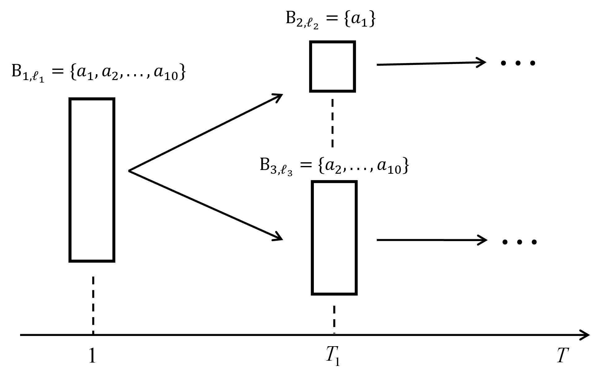
Figure 5: Process of the Algorithm 2 attacks BatchRank.

E.3 Proof of Theorem 3

The proof of Theorem 3 relies on the following Lemma 3.

Lemma 3.

The attacker utilizes Algorithm 2 to manipulate the returned click feedback of the BatchRank. After $16L\log(T)$ rounds attack and the BatchRank begins its first split. The upper confidence bound and lower confidence bound of every non-target item satisfies $L_{b,\ell_{1}}(a_{k})=0$ and $U_{b,\ell_{1}}(a_{k})=1-(T\log(T)^{3})^{-1/\displaystyle{\bm{n}}_{\ell_{1}}}$. The lower confidence bound and the upper confidence bound of the target item are $L_{b,\ell_{1}}(\tilde{a})=1$ and $U_{b,\ell_{1}}(\tilde{a})=1$.

Proof of Lemma 3.

According to the introduction of BatchRank, the estimated click probability of an arbitrary item is written as (24) and $\mathcal{C}_{b,\ell_{1}}(a_{k})$ is at most $16\log(T)$ in the first stage ($\ell_{1}=0$ and $\tilde{\Delta}_{\ell_{1}}^{-2}=2^{2\ell_{1}}=1$). Recall our attack Algorithm 2 returns $\tilde{\mathcal{C}}_{k}^{t}=0$ when $a_{k}\neq\tilde{a}$ and $a_{k}\in\mathcal{R}_{t}$. Thus, the total collected click number of the non-target item is $\mathcal{C}_{b,\ell_{1}}(a_{k})=0$, and the estimated click probability is $\hat{\mathcal{C}}_{b,\ell_{1}}(a_{k})=0$.

We first introduce the definition of the KL-divergence

$$\begin{split}D_{KL}(p\|q)=p\log(\frac{p}{q})+(1-p)\log(\frac{1-p}{1-q}).\end{split}$$ (26)

By convenience, we define $0\log(0)=0\log(0/0)=0$ and $x\log(x/0)=+\infty$ for $x>0$ (Garivier and Cappé, 2011). With this knowledge, we can derive the upper confidence bound of the non-target item in stage $\ell_{1}$

$$\begin{split}U_{b,\ell_{1}}(a_{k})&=\operatorname*{arg\,max}_{q\in[\hat{\mathcal{C}}_{b,\ell_{1}}(a_{k}),1]}\{\displaystyle{\bm{n}}_{\ell_{1}}D_{KL}(\hat{\mathcal{C}}_{b,\ell_{1}}(a_{k})\|q)\leq\log(T)+3\log\log(T)\}\\ &=\operatorname*{arg\,max}_{q\in[0,1]}\{\displaystyle{\bm{n}}_{\ell_{1}}(0\log\frac{0}{q}+1\log\frac{1}{1-q})\leq\log(T)+3\log\log(T)\}\\ &=\operatorname*{arg\,max}_{q\in[0,1]}\{\displaystyle{\bm{n}}_{\ell_{1}}\log\frac{1}{1-q}\leq\log(T)+3\log\log(T)\}.\end{split}$$ (27)

Apparently, when $q=1$, $\log(T)+3\log\log(T)\leq\displaystyle{\bm{n}}_{\ell_{1}}\log(1/1-q)=+\infty$, hence $q$ should smaller than $1$. When $\displaystyle{\bm{n}}_{\ell_{1}}\log(1/(1-q))=\log(T)+3\log\log(T)$, we have

$$\begin{split}\displaystyle{\bm{n}}_{\ell_{1}}\log(\frac{1}{1-q})&=\log(T\log(T)^{3})\\ \log(\frac{1}{1-q})&=\log\bigg{(}(T\log(T)^{3})^{1/\displaystyle{\bm{n}}_{\ell_{1}}}\bigg{)}\\ \frac{1}{1-q}&=(T\log(T)^{3})^{1/\displaystyle{\bm{n}}_{\ell_{1}}}\\ q&=1-(T\log(T)^{3})^{-1/\displaystyle{\bm{n}}_{\ell_{1}}}.\end{split}$$ (28)

Due to $T\log(T)^{3}>1$ and $\displaystyle{\bm{n}}_{\ell_{1}}>0$, we can derive $0<(T\log(T)^{3})^{-1/\displaystyle{\bm{n}}_{\ell_{1}}}<1$ and $0<U_{b,\ell_{1}}(a_{k})<1$.

The lower confidence bound of the non-target item has

$$L_{b,\ell_{1}}(a_{k}) =\operatorname*{arg\,min}_{q\in[0,0]}\{\displaystyle{\bm{n}}_{\ell_{1}}D_{KL}(\hat{\mathcal{C}}_{b,\ell_{1}}(a_{k})\|q)\leq\log(T)+3\log\log(T)\}=0.$$ (29)

Remember the attacker returns $\tilde{\mathcal{C}}_{k}^{t}=1$ if $a_{k}=\tilde{a}$ and $a_{k}\in\mathcal{R}_{t}$. Thus, the total collected click number of target item is $\mathcal{C}_{b,\ell_{1}}(\tilde{a})=16\log(T)$ and $\hat{\mathcal{C}}_{b,\ell_{1}}(\tilde{a})=1$. We can further deduce the upper confidence bound of the target item as

$$\begin{split}U_{b,\ell_{1}}(\tilde{a})&=\operatorname*{arg\,max}_{q\in[1,1]}\{\displaystyle{\bm{n}}_{\ell_{1}}D_{KL}(\hat{\mathcal{C}}_{b,\ell_{1}}(\tilde{a})\|q)\leq\log(T)+3\log\log(T)\}=1.\end{split}$$ (30)

The lower confidence bound of the target item has

$$\begin{split}L_{b,\ell_{1}}(\tilde{a})&=\operatorname*{arg\,min}_{q\in[0,1]}\{\displaystyle{\bm{n}}_{\ell_{1}}D_{KL}(\hat{\mathcal{C}}_{b,\ell_{1}}(\tilde{a})\|q)\leq\log(T)+3\log\log(T)\}=1\\ &=\operatorname*{arg\,min}_{q\in[0,1]}\{\displaystyle{\bm{n}}_{\ell_{1}}(1\log\frac{1}{q}+(1-1)\log\frac{1-1}{1-q})\leq\log(T)+3\log\log(T)\}\\ &=\operatorname*{arg\,min}_{q\in[0,1]}\{\displaystyle{\bm{n}}_{\ell_{1}}\log\frac{1}{q}\leq\log(T)+3\log\log(T)\}\\ &=1.\end{split}$$ (31)

Here finish the proof of Lemma 3. ∎

Proof of Theorem 3.

Consider the attacker implements attack Algorithm 2 with $T_{1}=16L\log(T)$. With the knowledge of Lemma 3, we can obtain when the BatchRank begins to split the first batch $B_{1,\ell_{1}}=\mathcal{D}$, the lower confidence bound of every non-target item satisfies $L_{b,\ell_{1}}(a_{k})=0$, and the lower confidence bound of the target item satisfies $L_{b,\ell_{1}}(\tilde{a})=1$. Therefore $\tilde{a}$ would be ranked at the first position because it has the highest lower confidence bound (line 6 in UpdateBatch). The BatchRank starts comparing $L_{b,\ell_{1}}(a_{k})$ and $\max_{a_{k}\in B_{k}^{-}}U_{b,\ell_{1}}(a_{k})$ for $k=1$ to $K-1$ (line 10 in UpdateBatch). Owing to $L_{b,\ell_{1}}(\tilde{a})=1>U_{b,\ell_{1}}(a_{k})$ and $L_{b,\ell_{1}}(a_{k})<U_{b,\ell_{1}}(a_{k})$, the split point is $s=1$ (line 11 in Updatebatch). After the split action, the BatchRank would derive two sub-batches $B_{2,\ell_{2}}=\{\tilde{a}\}$ and $B_{3,\ell_{3}}=\mathcal{D}\backslash\tilde{a}$. Sub-batch $B_{2,\ell_{2}}$ contains the first position of $\mathcal{R}_{t}$ (i.e., $\mathbb{a}_{1}^{t}$) and $B_{3,\ell_{3}}$ contains the rest of the positions of $\mathcal{R}_{t}$ (i.e., $\mathbb{a}_{2}^{t},...,\mathbb{a}_{K}^{t}$). Sub-batch $B_{2,\ell_{2}}$ would not split until round $T$ because it only contains a position and an item. This implies after round $16L\log(T)$, the target item would always be placed at the first position of $\mathcal{R}_{t}$ until round $T$ is over, i.e., $\mathds{E}[N_{T}(\tilde{a})]\geq T-16L\log(T)$. Due to the click number in each round being at most $K$, the cost in one round is at most $K$. Hence, the cost of Algorithm 2 can be bounded by $\mathcal{C}\leq KT_{1}$.

Based on the above results, we conclude that Algorithm 2 can efficiently attack BatchRank when $T_{1}=16L\log(T)$. Here finish the proof of Theorem 3. ∎

Appendix F Proof of Theorem 4

F.1 Introduction of TopRank

We here specifically illustrate details of the TopRank. The pseudo-code of the TopRank is provided.

Algorithm 8 The TopRank (Lattimore et al., 2018)

1:  Input: Graph $G_{1}=\emptyset$, round number $T$, $c=\frac{4\sqrt{2/\pi}}{\text{erf}(\sqrt{2})}\approx 3.43$

2:  for $t=1:T$ do

3:   Set $d=0$

4:   while $\mathcal{D}\backslash\bigcup_{c=1}^{d}\mathcal{P}_{tc}\neq\emptyset$ do

5:    Set $d=d+1$

6:    Set $\mathcal{P}_{td}=\min_{G_{t}}\Big{(}\mathcal{D}\backslash\bigcup_{c=1}^{d-1}\mathcal{P}_{tc}\Big{)}$

7:   Choose $\mathcal{R}_{t}$ uniformly at random from $\mathcal{P}_{t1},...,\mathcal{P}_{td}$

8:   Observe click feedback $\mathcal{C}_{t}=(\mathcal{C}_{1}^{t},...,\mathcal{C}_{L}^{t})$

9:   for $(i,j)\in[L]^{2}$ do

10:    if $a_{i},a_{j}\in\mathcal{P}_{td}$ for some $d$ then

11:     Set $U_{tij}=\mathcal{C}_{i}^{t}-\mathcal{C}_{j}^{t}$

12:    else

13:     Set $U_{tij}=0$

14:    Set $S_{tij}=\sum_{s=1}^{t}U_{tij}$ and $N_{tij}=\sum_{s=1}^{t}|U_{tij}|$

15:   Set $G_{t+1}=G_{t}\bigcup\Big{\{}(a_{j},a_{i}):S_{tij}\geq\sqrt{2N_{tij}\log(\frac{c}{\delta}\sqrt{N_{tij}})}$ and $N_{tij}>0\Big{\}}$

The TopRank would begin with a blank graph $G_{1}\subseteq[L]^{2}$. A directional edge $(a_{j},a_{i})\in G_{t}$ denotes the TopRank believes item $a_{i}$’s attractiveness is larger than item $a_{j}$. Let $\min_{G_{t}}(\mathcal{D}\backslash\bigcup_{c=1}^{d-1}\mathcal{P}_{tc})=\{a_{i}\in\mathcal{D}\backslash\bigcup_{c=1}^{d-1}\mathcal{P}_{tc}:(a_{i},a_{j})\not\in G_{t}\ \text{for}\ \text{all}\ a_{j}\in\mathcal{D}\backslash\bigcup_{c=1}^{d-1}\mathcal{P}_{tc}\}$. The algorithm would begin from round $1$ to round $T$. In each round, the TopRank would establish blocks $\mathcal{P}_{t1},...,\mathcal{P}_{td}$ via the graph $G_{t}$. Items in block $\mathcal{P}_{t1}$ would be placed randomly at the first $|\mathcal{P}_{t1}|$ positions in $\mathcal{R}_{t}$, and items in $\mathcal{P}_{t2}$ would be placed randomly at the next $|\mathcal{P}_{t2}|$ positions, and so on. In each round, after deriving click feedback $\mathcal{C}_{t}$, the TopRank would compute $U_{tij}=\mathcal{C}_{i}^{t}-\mathcal{C}_{j}^{t}$ if item $a_{i}$ and item $a_{j}$ are in the same block, otherwise, $U_{tij}=0$. Afterward, the TopRank would compute $S_{tij}=\sum_{s=1}^{t}U_{sij}$ and $N_{tij}=\sum_{s=1}^{t}|U_{sij}|$ and establish edge $(a_{j},a_{i})$ if $S_{tij}\geq\sqrt{2N_{tij}\log(\frac{c}{\delta}\sqrt{N_{tij}})}$ and $N_{tij}>0$. Without the attacker interference, the graph would not contain any cycle with probability at least $1-\delta L^{2}$, if the graph contains at least one cycle the TopRank would behave randomly (Lattimore et al., 2018). Parameter $\delta$ would be set as $\delta=1/T$.

F.2 Missing example in section 4.3

Example 3.

The process of the attack is shown in Figure 6. Consider the total item set $\mathcal{D}=\{a_{1},a_{2},a_{3}\}$ with $3$ items. The length of the list $\mathcal{R}_{t}$ is $K=2$ and the target item is $\tilde{a}=a_{1}$. The TopRank would start with block $\mathcal{P}_{11}=\mathcal{D}$ and $d=1$ because the graph contains no edges at the beginning. In the first $T_{1}$ rounds, the attacker receives click feedback $\mathcal{C}_{t}$ and modifies click feedback $\tilde{\mathcal{C}}_{k}^{t}=1$ if $a_{k}=\tilde{a}$ and $a_{k}\in\mathcal{R}_{t}$, otherwise $\tilde{\mathcal{C}}_{k}^{t}=0$. After $T_{1}$, the edges $(a_{k},\tilde{a}),\ k=2,3$ are established simultaneously. In the last $T-T_{1}$ rounds, the block $\mathcal{P}_{t1}$ would only contain $\tilde{a}$ and $\tilde{a}$ would always be placed at the first position of $\mathcal{R}_{t}$. Due to TopRank would only compare items’ attractiveness in the same block, the edges from $\tilde{a}$ to $a_{k}\neq\tilde{a}$ would never be established and cycle would appear in $G_{t}$ with very low probability (will be explained in the proof of Theorem 4 in the appendix).

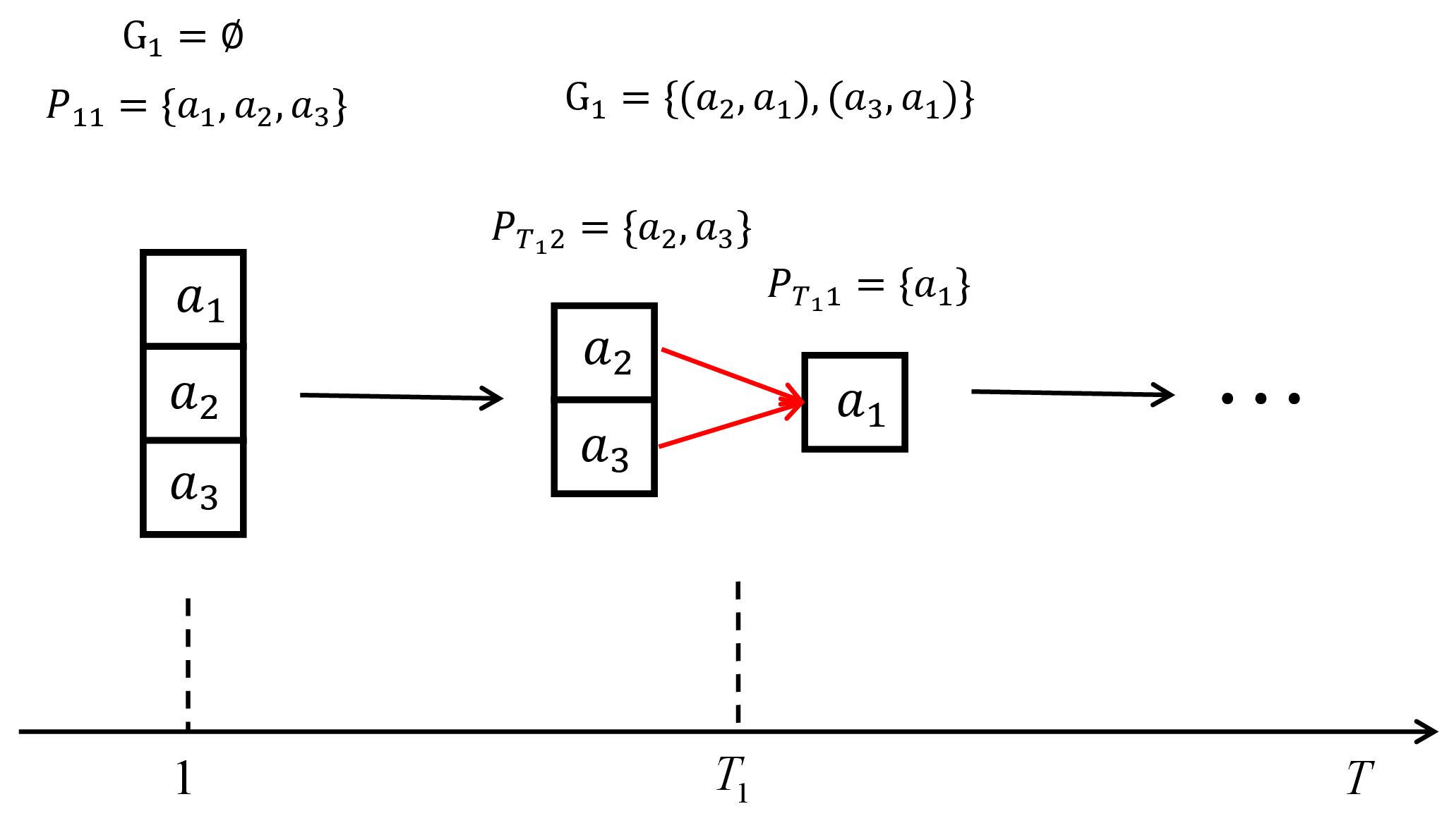
Figure 6: Process of the Algorithm 2 attacks TopRank.

F.3 Proof of Theorem 4

The proof of Theorem 4 relies on the following lemmas.

Lemma 4.

Consider the TopRank is under the attack of Algorithm 2. Denotes $a_{i}=\tilde{a}$ as the target item and $a_{j}\neq\tilde{a}$ as non-target items. When $\sum_{t=1}^{T_{1}}\mathds{1}\{\tilde{a}\in\mathcal{R}_{t}\}=4\log(c/\delta)$, then $S_{T_{1}ij}\geq\sqrt{2N_{T_{1}ij}\log(\frac{c}{\delta}\sqrt{N_{T_{1}ij}})}$ and $N_{T_{1}ij}>0$ are satisfied and edges from non-target items to target item (i.e., $(a_{j},a_{i})$, $a_{j}\not=a_{i}$) are established simultaneously.

Proof of Lemma 4.

Note that the TopRank sets $U_{tij}=\mathcal{C}_{i}^{t}-\mathcal{C}_{j}^{t}$ if $a_{i},a_{j}\in\mathcal{P}_{td}$ for some $d$, otherwise, $U_{tij}=0$. According to attack Algorithm 2, the TopRank would receive $\mathcal{C}_{i}^{t}=1$ ($\mathcal{C}_{i}^{t}$ is generates by the target item) if $\tilde{a}\in\mathcal{R}_{t}$ and $\mathcal{C}_{j}^{t}=0$ ($\mathcal{C}_{j}^{t}$ is generated by non-target items) when $t\leq T_{1}$. Based on this, we can derive

$$U_{tij}=\mathcal{C}^{t}_{i}-\mathcal{C}^{t}_{j}=1,\ t\leq T_{1},\ \tilde{a}\in\mathcal{R}_{t},\ a_{i},a_{j}\in\mathcal{P}_{td}.$$ (32)

Thus, when $\mathcal{P}_{t1}=\{\mathcal{D}\}$, we have

$$S_{tij}=\sum_{s=1}^{t}U_{tij}=N_{tij}=\sum_{s=1}^{t}|U_{tij}|=\sum_{s=1}^{t}\mathds{1}\{\tilde{a}\in\mathcal{R}_{t}\},\quad t\leq T_{1}.$$ (33)

In the light of (33) and line 15 of TopRank, if $\sum_{s=1}^{t}\mathds{1}\{\tilde{a}\in\mathcal{R}_{t}\}\geq\sqrt{2\sum_{s=1}^{t}\mathds{1}\{\tilde{a}\in\mathcal{R}_{t}\}\log(\frac{c}{\delta}\sqrt{\sum_{s=1}^{t}\mathds{1}\{\tilde{a}\in\mathcal{R}_{t}\}})}$, edges $(a_{j},a_{i})$ would establish. Utilizing the knowledge of the elementary algebra, we have

$$\begin{split}\sum_{s=1}^{t}\mathds{1}\{\tilde{a}\in\mathcal{R}_{t}\}&\geq\sqrt{2\sum_{s=1}^{t}\mathds{1}\{\tilde{a}\in\mathcal{R}_{t}\}\log\bigg{(}\frac{c}{\delta}\sqrt{\sum_{s=1}^{t}\mathds{1}\{\tilde{a}\in\mathcal{R}_{t}\}}\bigg{)}}\\ \bigg{(}\sum_{s=1}^{t}\mathds{1}\{\tilde{a}\in\mathcal{R}_{t}\}\bigg{)}^{2}&\geq 2\sum_{s=1}^{t}\mathds{1}\{\tilde{a}\in\mathcal{R}_{t}\}\Bigg{(}\log(\frac{c}{\delta})+\log\bigg{(}\sqrt{\sum_{s=1}^{t}\mathds{1}\{\tilde{a}\in\mathcal{R}_{t}\}}\bigg{)}\Bigg{)}\\ \frac{1}{2}\sum_{s=1}^{t}\mathds{1}\{\tilde{a}\in\mathcal{R}_{t}\}-\log\bigg{(}\sqrt{\sum_{s=1}^{t}\mathds{1}\{\tilde{a}\in\mathcal{R}_{t}\}}\bigg{)}&\geq\log(\frac{c}{\delta})\\ \sum_{s=1}^{t}\mathds{1}\{\tilde{a}\in\mathcal{R}_{t}\}&\geq 4\log(\frac{c}{\delta}).\end{split}$$ (34)

The second inequality holds because of $\sum_{s=1}^{t}\mathds{1}\{\tilde{a}\in\mathcal{R}_{t}\}>0$. The fourth inequality holds because of $(1/4)x>log(\sqrt{x})$ when $x>0$. Thus, when $\sum_{s=1}^{t}\mathds{1}\{\tilde{a}\in\mathcal{R}_{t}\}\geq 4\log(c/\delta)$ and $t\leq T_{1}$, edges $(a_{j},a_{i})$ would establish simultaneously. We here finish the proof of Lemma 4. ∎

Lemma 5.

Suppose input $T_{1}=\frac{4\log(c/\delta)}{\frac{K}{L}+(1-\sqrt{1+8K/L})/4}$, then with probability at least $1-\delta/c$, the TopRank would achieve $\sum_{t=1}^{T_{1}}\mathds{1}\{\tilde{a}\in\mathcal{R}_{t}\}>4\log(c/\delta)$.

Proof of Lemma 5.

According to the previous discussion, we can separate $T_{1}$ into two periods $P_{1}$ and $P_{2}$ (i.e., $T_{1}=P_{1}+P_{2}$). In period one $G_{t}=\emptyset$ and in period two $G_{t}$ only contains edges from non-target items to the target item. Based on the TopRank property, in period one $P(\tilde{a}\in\mathcal{R}_{t}|t\leq P_{1})=K/L$ and in period two $P(\tilde{a}\in\mathcal{R}_{t}|P_{1}+1\leq t\leq T_{1})=1$. Define a Bernoulli distribution $X$ that satisfies $X=1$ with probability $K/L$. With the help of the Hoeffding inequality, we can derive

$$P\bigg{(}\sum_{t=1}^{T_{1}}X_{t}-\frac{K}{L}T_{1}\leq-aT_{1}\bigg{)}\leq e^{-T_{1}a^{2}/2}.$$ (35)

Set $T_{1}=\frac{4\log(c/\delta)}{\frac{K}{L}+(1-\sqrt{1+8K/L})/4}$ and $a=-(1-\sqrt{1+8K/L})/4$. We can derive

$$P\bigg{(}\sum_{t=1}^{T_{1}}X_{t}\leq 4\log(c/\delta)\bigg{)}\leq\frac{\delta}{c}.$$ (36)

Further derivation shows that

$$P\bigg{(}\sum_{t=1}^{T_{1}}X_{t}>4\log(c/\delta)\bigg{)}>1-\frac{\delta}{c}.$$ (37)

Follows the definition of the TopRank, one has

$$\begin{split}P\bigg{(}\sum_{t=1}^{P_{1}}\mathds{1}\{\tilde{a}\in\mathcal{R}_{t}\}+\sum_{t=P_{1}+1}^{T_{1}}\mathds{1}\{\tilde{a}\in\mathcal{R}_{t}\}>4\log(c/\delta)\bigg{)}&=P\bigg{(}\sum_{t=1}^{P_{1}}\mathds{1}\{\tilde{a}\in\mathcal{R}_{t}\}+P_{2}>4\log(c/\delta)\bigg{)}\\ &\geq P\bigg{(}\sum_{t=1}^{T_{1}}X_{t}>4\log(c/\delta)\bigg{)}\end{split}$$ (38)

where the first equation holds because $\sum_{t=P_{1}+1}^{T_{1}}\mathds{1}\{\tilde{a}\in\mathcal{R}_{t}\}=P_{2}$. The last inequality holds because $P_{2}\geq\sum_{t=P_{1}+1}^{T_{1}}X_{t}$. Combining (37) and (38), we can finally get

$$P\bigg{(}\sum_{t=1}^{T_{1}}\mathds{1}\{\tilde{a}\in\mathcal{R}_{t}\}\geq 4\log(c/\delta)\bigg{)}>1-\frac{\delta}{c}$$ (39)

when $T_{1}=\frac{4\log(c/\delta)}{\frac{K}{L}+(1-\sqrt{1+8K/L})/4}$. Here finish the proof of Lemma 5. ∎

Lemma 6.

If the attacker implements attack Algorithm 2 and $T_{1}=\frac{4\log(c/\delta)}{\frac{K}{L}+(1-\sqrt{1+8K/L})/4}$, the graph $G_{t}$ would not contain any cycle with probability at least $1-(L^{2}+1/c)\delta$.

Proof of Lemma 6.

We here analyze our attack Algorithm 2 would not case $G_{t}$ contains any cycle with high probability if the input $T_{1}=\frac{4\log(c/\delta)}{\frac{K}{L}+(1-\sqrt{1+8K/L})/4}$. Consider the attacker implementing our attack strategy from round $1$ to round $T_{1}$. Define $a_{i}=\tilde{a}$ and $a_{j}\neq\tilde{a}$. The attacker frauds the TopRank to believe the target item $\tilde{a}$ is clicked $\sum_{t=1}^{T_{1}}\mathds{1}\{\tilde{a}\in\mathcal{R}_{t}\}$ times and non-target items are clicked 0 time in $T_{1}$. After $S_{tij}\geq\sqrt{2N_{tij}\log(\frac{c}{\delta}\sqrt{N_{tij}})}$ and $N_{tij}>0$ are satisfied, the edges would be established at the same time and $\tilde{a}$ would belong to the first block (line 6 in the TopRank and Lemma 4 and 6). Note that during $T_{1}$, the attacker sets $\mathcal{C}_{j}^{t}=0$. Thus

$$\begin{split}N_{T_{1}ji}&=\sum_{t=1}^{T_{1}}|U_{tji}|=\sum_{t=1}^{T_{1}}|\mathcal{C}_{j}^{t}-\mathcal{C}_{i}^{t}|=\sum_{t=1}^{T_{1}}\mathds{1}\{\tilde{a}\in\mathcal{R}_{t}\}\\ S_{T_{1}ji}&=\sum_{t=1}^{T_{1}}U_{tji}=\sum_{t=1}^{T_{1}}(\mathcal{C}_{j}^{t}-\mathcal{C}_{i}^{t})=-\sum_{t=1}^{T_{1}}\mathds{1}\{\tilde{a}\in\mathcal{R}_{t}\}.\end{split}$$ (40)

Since $U_{tij}$ and $U_{tji}$ would be $0$ after $t>T_{1}$ (line 9-13 in TopRank), we can obtain $S_{T_{1}ji}=-\sum_{t=1}^{T_{1}}\mathds{1}\{\tilde{a}\in\mathcal{R}_{t}\}$ and $N_{T_{1}ji}=\sum_{t=1}^{T_{1}}\mathds{1}\{\tilde{a}\in\mathcal{R}_{t}\}$ hold when $t>T_{1}$. This implies the directional edges from the target item to non-target items would never establish, i.e., $-\sum_{t=1}^{T_{1}}\mathds{1}\{\tilde{a}\in\mathcal{R}_{t}\}<\sqrt{2\sum_{t=1}^{T_{1}}\mathds{1}\{\tilde{a}\in\mathcal{R}_{t}\}\log(\frac{c}{\delta}\sqrt{\sum_{t=1}^{T_{1}}\mathds{1}\{\tilde{a}\in\mathcal{R}_{t}\}})}$). Besides, due to the received click number from non-target items being $0$ in $T_{1}$, the $S_{T_{1}}$ and $N_{T_{1}}$ between non-target items would be $0$. This implies the manipulation of the attacker would not influence the TopRank judgment of the attractiveness between non-target items. In other words, the TopRank under Algorithm 2 attack can be considered as the TopRank interacts with item set $\mathcal{D}\backslash\tilde{a}$ in $T-T_{1}$ rounds.

According to the above discussion and Lemma 5, if $T_{1}=\frac{4\log(c/\delta)}{\frac{K}{L}+(1-\sqrt{1+8K/L})/4}$, then $S_{T_{1}ij}\geq\sqrt{2N_{T_{1}ij}\log(\frac{c}{\delta}\sqrt{N_{T_{1}ij}})}$ would satisfy with probability at least $1-\delta/c$. Besides, from round $T_{1}+1$ to $T$, cycles would occur with probability at most $\delta L^{2}$. Thus graph $G_{t}$ would not contain cycles with probability at least $1-(L^{2}+1/c)\delta$ until $T$. ∎

Proof of Theorem 4.

Suppose the attacker implements attack Algorithm 2 with input value $T_{1}=\frac{4\log(c/\delta)}{\frac{K}{L}+(1-\sqrt{1+8K/L})/4}$. Then, the TopRank would establish edges from non-target items to $\tilde{a}$ with probability at least $1-\delta/c$ (According to Lemma 4 and Lemma 5). Based on the analysis in Lemma 6, the cycle would appear with probability at most $(L^{2}+1/c)\delta$ and the first block would only contain $\tilde{a}$ till $T$. That is to say, the target item in block $\mathcal{P}_{t1}$ would always be placed at the first positions after $T_{1}$ with probability at least $1-(L^{2}+1/c)\delta$. Following Algorithm 2, the attacker would only manipulate the returned click feedback for $T_{1}$ times. Thus the attack cost can be bounded by $\mathcal{C}(T)\leq KT_{1}$.

According to the above observation, we summarize that Algorithm 2 can efficiently attack TopRank when $T_{1}=\frac{4\log(c/\delta)}{\frac{K}{L}+(1-\sqrt{1+8K/L})/4}$. Here finish the proof of Theorem 4. ∎

References

- Auer et al. (2002) Peter Auer, Nicolo Cesa-Bianchi, and Paul Fischer. Finite-time analysis of the multiarmed bandit problem. Machine learning, 47(2-3):235–256, 2002.
- Bogunovic et al. (2021) Ilija Bogunovic, Arpan Losalka, Andreas Krause, and Jonathan Scarlett. Stochastic linear bandits robust to adversarial attacks. In International Conference on Artificial Intelligence and Statistics, pages 991–999. PMLR, 2021.
- BuzzFeed (2019) BuzzFeed. Some amazon sellers are paying 10,000 a month to trick their way to the top. 2019.
- Chuklin et al. (2015) Aleksandr Chuklin, Ilya Markov, and M. de Rijke. Click models for web search. In Click Models for Web Search, 2015.
- Craswell et al. (2008) Nick Craswell, Onno Zoeter, Michael J. Taylor, and Bill Ramsey. An experimental comparison of click position-bias models. In Web Search and Data Mining, 2008.
- Even-Dar et al. (2006) Eyal Even-Dar, Shie Mannor, and Y. Mansour. Action elimination and stopping conditions for the multi-armed bandit and reinforcement learning problems. J. Mach. Learn. Res., 7:1079–1105, 2006.
- Garcelon et al. (2020) Evrard Garcelon, Baptiste Roziere, Laurent Meunier, Jean Tarbouriech, Olivier Teytaud, Alessandro Lazaric, and Matteo Pirotta. Adversarial attacks on linear contextual bandits. Advances in Neural Information Processing Systems, 33, 2020.
- Garivier and Cappé (2011) Aurélien Garivier and Olivier Cappé. The kl-ucb algorithm for bounded stochastic bandits and beyond. In Annual Conference Computational Learning Theory, 2011.
- Gauthier et al. (2022) Camille-Sovanneary Gauthier, R. Gaudel, and Élisa Fromont. Unirank: Unimodal bandit algorithms for online ranking. ArXiv, abs/2208.01515, 2022.
- Golrezaei et al. (2021) Negin Golrezaei, Vahideh Manshadi, Jon Schneider, and Shreyas Sekar. Learning product rankings robust to fake users. Proceedings of the 22nd ACM Conference on Economics and Computation, 2021.
- Grotov and de Rijke (2016) Artem Grotov and Maarten de Rijke. Online learning to rank for information retrieval: Sigir 2016 tutorial. In Proceedings of the 39th International ACM SIGIR conference on Research and Development in Information Retrieval, pages 1215–1218. ACM, 2016.
- Harper and Konstan (2016) F. Maxwell Harper and Joseph A. Konstan. The movielens datasets: History and context. ACM Trans. Interact. Intell. Syst., 5:19:1–19:19, 2016.
- Jia et al. (2021) Yiling Jia, Huazheng Wang, Stephen Guo, and Hongning Wang. Pairrank: Online pairwise learning to rank by divide-and-conquer. In Proceedings of the Web Conference 2021, pages 146–157, 2021.
- Jun et al. (2018) Kwang-Sung Jun, Lihong Li, Yuzhe Ma, and Jerry Zhu. Adversarial attacks on stochastic bandits. In Advances in Neural Information Processing Systems, pages 3640–3649, 2018.
- Katariya et al. (2016) Sumeet Katariya, Branislav Kveton, Csaba Szepesvari, and Zheng Wen. Dcm bandits: Learning to rank with multiple clicks. In International Conference on Machine Learning, pages 1215–1224, 2016.
- Kveton et al. (2015a) Branislav Kveton, Csaba Szepesvari, Zheng Wen, and Azin Ashkan. Cascading bandits: Learning to rank in the cascade model. In International Conference on Machine Learning, 2015a.
- Kveton et al. (2015b) Branislav Kveton, Zheng Wen, Azin Ashkan, and Csaba Szepesvari. Combinatorial cascading bandits. In NIPS, 2015b.
- Lagrée et al. (2016) Paul Lagrée, Claire Vernade, and Olivier Cappé. Multiple-play bandits in the position-based model. In NIPS, 2016.
- Lattimore et al. (2018) Tor Lattimore, Branislav Kveton, Shuai Li, and Csaba Szepesvari. Toprank: A practical algorithm for online stochastic ranking. In NeurIPS, 2018.
- Li et al. (2018) Chang Li, Branislav Kveton, Tor Lattimore, Ilya Markov, M. de Rijke, Csaba Szepesvari, and Masrour Zoghi. Bubblerank: Safe online learning to re-rank via implicit click feedback. In Conference on Uncertainty in Artificial Intelligence, 2018.
- Li et al. (2016) Shuai Li, Baoxiang Wang, Shengyu Zhang, and Wei Chen. Contextual combinatorial cascading bandits. In International Conference on Machine Learning, pages 1245–1253, 2016.
- Li et al. (2019) Shuai Li, Tor Lattimore, and Csaba Szepesvari. Online learning to rank with features. ArXiv, abs/1810.02567, 2019.
- Liu and Shroff (2019) Fang Liu and Ness Shroff. Data poisoning attacks on stochastic bandits. In International Conference on Machine Learning, pages 4042–4050, 2019.
- Liu and Lai (2020) Guanlin Liu and Lifeng Lai. Action-manipulation attacks on stochastic bandits. ICASSP 2020 - 2020 IEEE International Conference on Acoustics, Speech and Signal Processing (ICASSP), pages 3112–3116, 2020.
- Liu and Lai (2021) Guanlin Liu and Lifeng Lai. Efficient action poisoning attacks on linear contextual bandits. ArXiv, abs/2112.05367, 2021.
- Liu et al. (2009) Tie-Yan Liu et al. Learning to rank for information retrieval. Foundations and Trends® in Information Retrieval, 3(3):225–331, 2009.
- Liu et al. (2018) Weiwen Liu, Shuai Li, and Shengyu Zhang. Contextual dependent click bandit algorithm for web recommendation. In International Computing and Combinatorics Conference, 2018.
- Lykouris et al. (2018) Thodoris Lykouris, Vahab Mirrokni, and Renato Paes Leme. Stochastic bandits robust to adversarial corruptions. In Proceedings of the 50th Annual ACM SIGACT Symposium on Theory of Computing, pages 114–122. ACM, 2018.
- Oosterhuis and de Rijke (2018) Harrie Oosterhuis and Maarten de Rijke. Differentiable unbiased online learning to rank. Proceedings of the 27th ACM International Conference on Information and Knowledge Management - CIKM ’18, 2018. doi: 10.1145/3269206.3271686. URL http://dx.doi.org/10.1145/3269206.3271686.
- Ouni et al. (2022) Achref Ouni, Eric Royer, Thierry Chateau, Marc Chevaldonné, and Michel Dhome. Deep learning for robust information retrieval system. In International Conference on Computational Collective Intelligence, 2022.
- Radlinski et al. (2008) Filip Radlinski, Madhu Kurup, and Thorsten Joachims. How does clickthrough data reflect retrieval quality? In CIKM ’08, 2008.
- Richardson et al. (2007) Matthew Richardson, Ewa Dominowska, and Robert J. Ragno. Predicting clicks: estimating the click-through rate for new ads. In The Web Conference, 2007.
- Slivkins et al. (2013) Aleksandrs Slivkins, Filip Radlinski, and Sreenivas Gollapudi. Ranked bandits in metric spaces: learning diverse rankings over large document collections. J. Mach. Learn. Res., 14:399–436, 2013.
- Sun and Jafar (2016) Hua Sun and Syed Ali Jafar. The capacity of robust private information retrieval with colluding databases. IEEE Transactions on Information Theory, 64:2361–2370, 2016.
- Vial et al. (2022) Daniel Vial, S. Sanghavi, Sanjay Shakkottai, and Rayadurgam Srikant. Minimax regret for cascading bandits. ArXiv, abs/2203.12577, 2022.
- Wang et al. (2019) Huazheng Wang, Sonwoo Kim, Eric McCord-Snook, Qingyun Wu, and Hongning Wang. Variance reduction in gradient exploration for online learning to rank. In Proceedings of the 42nd International ACM SIGIR Conference on Research and Development in Information Retrieval, pages 835–844, 2019.
- Wang et al. (2022) Huazheng Wang, Haifeng Xu, and Hongning Wang. When are linear stochastic bandits attackable? In International Conference on Machine Learning, pages 23254–23273. PMLR, 2022.
- WSJ (2018) WSJ. How sellers trick amazon to boost sales. 2018.
- Xu et al. (2021) Ying Xu, Bhuvesh Kumar, and Jacob D. Abernethy. Observation-free attacks on stochastic bandits. In NeurIPS, 2021.
- Zoghi et al. (2017) Masrour Zoghi, Tomas Tunys, Mohammad Ghavamzadeh, Branislav Kveton, Csaba Szepesvari, and Zheng Wen. Online learning to rank in stochastic click models. In International Conference on Machine Learning, pages 4199–4208, 2017.
- Zong et al. (2016) Shi Zong, Hao Ni, Kenny Sung, Nan Rosemary Ke, Zheng Wen, and Branislav Kveton. Cascading bandits for large-scale recommendation problems. ArXiv, abs/1603.05359, 2016.