dotears: Scalable, consistent DAG estimation using observational and interventional data

Albert Xue1  Jingyou Rao1  Sriram Sankararaman1∗  Harold Pimentel1∗
1University of California, Los Angeles
{asxue, roserao, hjp}@ucla.edu
sriram@cs.ucla.edu
Abstract

Learning causal directed acyclic graphs (DAGs) from data is complicated by a lack of identifiability and the combinatorial space of solutions. Recent work has improved tractability of score-based structure learning of DAGs in observational data, but is sensitive to the structure of the exogenous error variances. On the other hand, learning exogenous variance structure from observational data requires prior knowledge of structure. Motivated by new biological technologies that link highly parallel gene interventions to a high-dimensional observation, we present dotears [doo-tairs], a scalable structure learning framework which leverages observational and interventional data to infer a single causal structure through continuous optimization. dotears exploits predictable structural consequences of interventions to directly estimate the exogenous error structure, bypassing the circular estimation problem. We extend previous work to show, both empirically and analytically, that the inferences of previous methods are driven by exogenous variance structure, but dotears is robust to exogenous variance structure. Across varied simulations of large random DAGs, dotears outperforms state-of-the-art methods in structure estimation. Finally, we show that dotears is a provably consistent estimator of the true DAG under mild assumptions.

**footnotetext: These authors contributed equally to this work.

1 Introduction

Causal structure learning considers the problem of learning causal relationships between variables in the form of a Directed Acyclic Graph (DAG). Inferring causal structure from data disentangles causal from correlational relationships, and is therefore helpful to understanding problems in fields ranging from protein signaling and genetics to finance [1, 2, 3].

Identifiability and tractability are the primary difficulties in learning DAGs from data. For identifiability, two distinct DAGs contain the same conditional independence relationships under observational data, and DAGs are therefore only identifiable up to Markov equivalence [4, 5, 6]. Here we contrast observational data with interventional data, and characterize observational data as data with no interventions made to the system. For tractability, the search space of DAGs grows combinatorially in the number of nodes, and learning DAGs from data is therefore NP-hard [7, 8, 9].

Recent work has improved tractability of the structure learning problem. DAGs with NO TEARS introduces a continuous, differentiable acyclicity constraint, which avoids combinatorial characterizations of DAGs and allows for continuous optimization of structure [10]. In simulations, however, NO TEARS infers DAGs with high “varsortability", where varsortability measures the “agreement between the order of increasing marginal variance and the [topological] order" [11]. NO TEARS estimates are therefore sensitive to exogenous variance structure, edge weight magnitude, or even simple re-scaling and unit measurement conversion, further complicating identifiability [11].

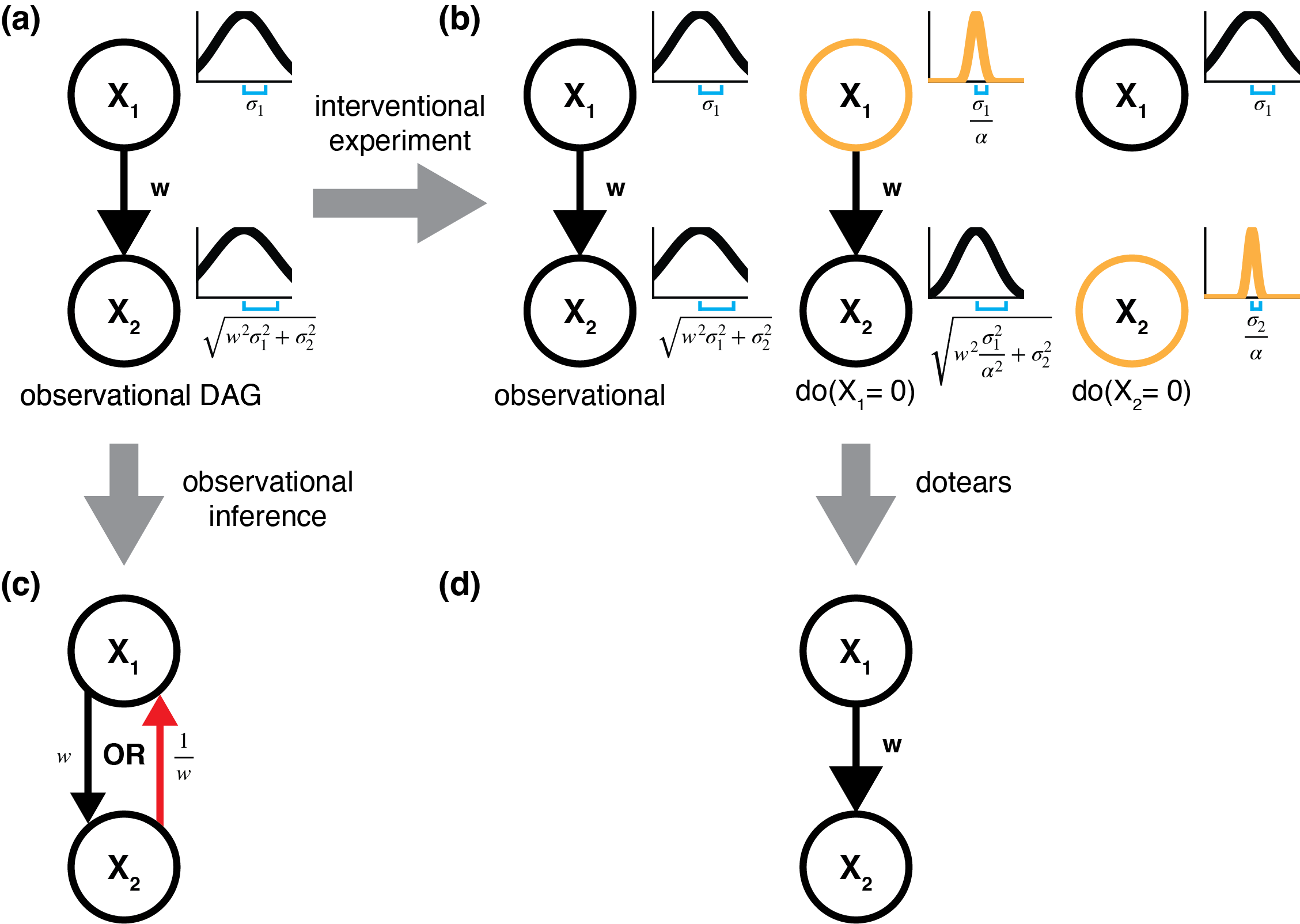
We argue that any loss function modeling the linear Structural Equation Model (SEM) without accounting for the exogenous variance is similarly limited. Specifically, let $X$ be a $p$-dimensional random vector, $W_{0}\in\mathbb{R}^{p\times p}$ the unknown weighted adjacency matrix of the true DAG, and $\epsilon$ an unknown $p$-dimensional random vector specifying the exogenous error. Then the linear SEM gives the autoregressive formulation

$$X=XW_{0}+\epsilon,\quad\Omega_{0}\coloneqq\text{Cov}\left(\epsilon\right).$$

Under this linear SEM, the two unknowns $W_{0}$ and $\Omega_{0}$ form an interdependent relationship that determines the marginal variance structure of $X$ (Figure 1).

We first explore the impact of using a least squares loss (as used in NO TEARS) for inference in this model. In the non-trivial two node case, we extend previous work[12] to derive a bound on correct inference. Our bound is a function of the effect size and the ratio between the exogenous variances, and also holds if and only if the system is varsortable – one whose topological ordering is identical to the ordering based on increasing marginal variance. In simulations, we verify the relationship between varsortable systems and correct inference, and demonstrate that our findings generalize beyond the least squares loss.

We further argue that issues of interdependence between $W_{0}$ and $\Omega_{0}$ are inseparable from the use of observational data for structure estimation. In observational data, we have a circular estimation problem, where without knowledge of $\Omega_{0}$ we cannot marginally infer $W_{0}$, and without knowledge of $W_{0}$ we cannot marginally infer $\Omega_{0}$. Despite these and other limitations, observational studies have been used for causal inference because of the difficulty and cost in obtaining interventional data.

Inspired by recent high-throughput genomic technologies that link high-dimensional observations to highly parallel known interventions [13, 14, 15], we present dotears, a novel optimization framework for structure learning. dotears extends the NO TEARS framework for continuous optimization on DAGs through 1.) a novel marginal estimation procedure for $\Omega_{0}$ using the structural consequences of interventions, and 2.) joint estimation of the causal DAG from observational and interventional data, given the estimated $\Omega_{0}$. In simulations, dotears outperforms all other tested state-of-the-art methods and is robust to exogenous variance structure. Further, we show that dotears is a consistent estimator of the true DAG under mild assumptions by extending results from [16].

Refer to caption
Figure 1: dotears uses both observational and interventional data to identify the true DAG, while methods only using observational data can only identify the true DAG up to Markov Equivalency. Patterns in marginal variance affect continuous optimization methods on observational data. Interventional experiments can be done through high-throughput CRISPR screens like Perturb-seq [13]. (a) The true observational DAG $X_{1}\overset{w}{\to}X_{2}$, with corresponding distributions. (b) Interventions on node $k$ remove incoming edges to $k$. Upon intervention, the marginal variance shrinks due to removal of upstream variance and effects from the intervention. (c) NO TEARS cannot effectively distinguish between members of the Markov Equivalence class of the DAG in (a), and in fact infers as a deterministic function of $\sigma_{1}^{2}$ and $\sigma_{2}^{2}$ (see Figure 2). (d) dotears estimates exogenous variance from interventional data to robustly infer the true DAG.

2 Formulation

Let $G=\left([p],\,\mathcal{E}\right)$ a DAG on $p$ nodes with node set $[p]\coloneqq\{1\dots p\}$ and edge set $\mathcal{E}$. We represent $\mathcal{E}$ with the weighted adjacency matrix $W\in\mathcal{D}\subset\mathbb{R}^{p\times p}$, where $\mathcal{D}\subset\mathbb{R}^{p\times p}$ is the set of weighted adjacency matrices on $p$ nodes whose support is a DAG. We denote the parent set of node $i$ in the observational setting as $\text{Pa}(i)$. For $w_{ij}$ the $i,j$ entry in $W$, $|w_{ij}|>0$ indicates an edge $i\rightarrow j$ with weight $w_{ij}$, equivalently denoted $i\overset{w_{ij}}{\rightarrow}j$. $k=0,1,\dots,p$ indexes the intervention, where $k=0$ is reserved for the observational system, and $k\neq 0$ denotes intervention on node $k$. Similarly, we denote $\left(\cdot\right)^{(0)}$ for observational quantities, and $\left(\cdot\right)^{(k)}$ for quantities under intervention on node $k$. For brevity, a variable without a superscript is assumed to be observational; for example, $X\equiv X^{(0)}$. $\boldsymbol{X}$ (bolded) denotes $n_{0}$ samples drawn from the (unbolded) $p$-dimensional random vector $X$, and $\boldsymbol{\epsilon}$ (bolded) denotes $n_{0}$ samples drawn from the (unbolded) $p$-dimensional random vector $\epsilon$. Similarly, if $X^{(k)}$ is a $p$-dimensional random vector, then $\boldsymbol{X}^{(k)}\in\mathbb{R}^{n_{k}\times p}$ represents $n_{k}$ observations of $X$. We denote the total sample size $n\coloneqq\sum_{k=0}^{p}n_{k}$, and the true weighted adjacency matrix $W_{0}$.

The linear SEM is an autoregressive representation of $X^{(k)}$ and weighted adjacency matrix $W_{0}^{(k)}$,

$$X^{(k)}=X^{(k)}W_{0}^{(k)}+\epsilon^{(k)},\quad k=0,\dots,p.$$ (1)

Here, $W_{0}^{(k)}$ is permutation-similar to a strictly upper triangular matrix, representing the constraint $W_{0}^{(k)}\in\mathcal{D}$. For each $k$, $\epsilon^{(k)}$ is a $p$-dimensional random vector such that $\mathbb{E}\epsilon^{(k)}=0_{p}$, $\Omega_{0}^{(k)}\coloneqq\text{Cov}(\epsilon^{(k)})$, and $\epsilon^{(k)}\mathchoice{\mathrel{\hbox to0.0pt{$\displaystyle\perp$\hss}\mkern 2.0mu{\displaystyle\perp}}}{\mathrel{\hbox to0.0pt{$\textstyle\perp$\hss}\mkern 2.0mu{\textstyle\perp}}}{\mathrel{\hbox to0.0pt{$\scriptstyle\perp$\hss}\mkern 2.0mu{\scriptstyle\perp}}}{\mathrel{\hbox to0.0pt{$\scriptscriptstyle\perp$\hss}\mkern 2.0mu{\scriptscriptstyle\perp}}}X^{(k)}$. Denote $\epsilon_{i}$ as the $i$th element of $\epsilon$. Then $\epsilon_{i}^{(k)}$ is the exogenous error on node $i$, such that $\mathbb{E}\epsilon_{i}^{(k)}=0$ and $\epsilon_{i}^{(k)}\mathchoice{\mathrel{\hbox to0.0pt{$\displaystyle\perp$\hss}\mkern 2.0mu{\displaystyle\perp}}}{\mathrel{\hbox to0.0pt{$\textstyle\perp$\hss}\mkern 2.0mu{\textstyle\perp}}}{\mathrel{\hbox to0.0pt{$\scriptstyle\perp$\hss}\mkern 2.0mu{\scriptstyle\perp}}}{\mathrel{\hbox to0.0pt{$\scriptscriptstyle\perp$\hss}\mkern 2.0mu{\scriptscriptstyle\perp}}}\epsilon_{j}^{(k)}$ for $i\neq j$. We further define

$\displaystyle\Omega_{0}$ $\displaystyle\coloneqq\text{Cov}(\epsilon^{(0)})$
$\displaystyle=\text{diag}\left(\sigma_{1}^{2},\sigma_{2}^{2},\cdots,\sigma_{p}^{2}\right).$

Under Eq. 1, $W_{0}$ and $\Omega_{0}$ determine the marginal variance of $X_{j}$. In particular, for a node $j$

$$\text{Var}\left(X_{j}\right)=\sum_{i=1}^{p}w_{ij}^{2}\text{Var}(X_{i})+\sigma_{j}^{2},$$

and $\text{Var}(X_{j})=\sigma_{j}^{2}$ if and only if $|w_{ij}|=0\,\,\forall i\in[p]$, or equivalently when $j$ is a source node.

3 Related work

DAGs with NO TEARS [10] transforms the combinatorial constraint $W\in\mathcal{D}$ into the continuous constraint $h(W)=0$, where

$$h(W)=\textrm{tr}\left[\exp\left({W\circ W}\right)\right]-p$$

for $\circ$ the Hadamard product. Define $\|\cdot\|_{1}$ as the vector $\ell_{1}$ norm on $\text{vec}\left(W\right)$, i.e. $\|\text{vec}\left(W\right)\|_{1}$, and $\left|\left|{\cdot}\right|\right|_{F}$ the Frobenius norm. The differentiability of $h$ allows for the optimization framework

$$\begin{aligned} \min_{W}&\,\,\frac{1}{2n_{0}}\left|\left|\boldsymbol{X}-\boldsymbol{X}W\right|\right|_{F}^{2}+\lambda\|W\|_{1}\\ \text{s.t.}&\,\,h(W)=0\end{aligned}.$$ (2)

3.1 The least squares loss is equivalent to varsortability

The loss function $\left|\left|\boldsymbol{X}-\boldsymbol{X}W\right|\right|_{F}^{2}$ follows naturally from the SEM formulation $X=XW+\epsilon$, and is equivalent to the least squares formulation [10, 16]. However, we show that the least squares loss deterministically infers varsortable structures in the simplest non-trivial DAG $X_{1}\overset{w}{\rightarrow}X_{2}$. Assume $X_{1}\overset{w}{\to}X_{2}$ has true weighted adjacency matrix $W_{0}\coloneqq\begin{pmatrix}0&w\\ 0&0\end{pmatrix}$ and SEM

$\displaystyle X_{1}$ $\displaystyle=\epsilon_{1},$ $\displaystyle\text{Var}\left(\epsilon_{1}\right)=\sigma_{1}^{2},$ (3)
$\displaystyle X_{2}$ $\displaystyle=wX_{1}+\epsilon_{2},$ $\displaystyle\text{Var}\left(\epsilon_{2}\right)=\sigma_{2}^{2}.$

Kaiser and Sipos (2022) show that, in expectation, the least squares loss infers correctly when $|w|\geq 1$, under the assumption $\sigma_{2}^{2}=0$ [12]. We obtain a more general bound in the variance ratio $\gamma\coloneqq\frac{\sigma_{1}^{2}}{\sigma_{2}^{2}}$, and recover the previous as $\gamma\to\infty$.

Lemma 1.

Let $\gamma\coloneqq\frac{\sigma_{1}^{2}}{\sigma_{2}^{2}}$. The system $X_{1}\overset{w}{\rightarrow}X_{2}$ is varsortable if and only if $|w|\geq\sqrt{1-\frac{1}{\gamma}}$.

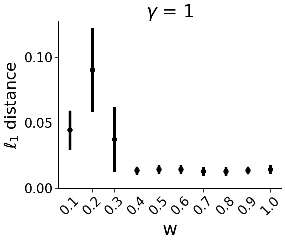
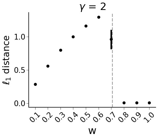
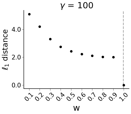
For the proof, see Supplementary Material 7.1.1. Figure 2 shows the performance of NO TEARS without $\ell_{1}$ regularization on simulated Gaussian data across a range of $w,\gamma$, for the generative model in Eq. 3. NO TEARS infers structure correctly only when $|w|\geq\sqrt{1-\frac{1}{\gamma}}$, matching Lemma 1. For simulation details and results on all simulated values of $w$ and $\gamma$, see Supplementary Material 7.4.

Refer to caption
(a) Under the equal variance assumption $\gamma=1$, NO TEARS will infer correctly for all $w$.
Refer to caption
(b) At $\gamma=2$, the bound $\sqrt{1-\frac{1}{\gamma}}\approx 0.7$. NO TEARS infers incorrectly when $w<0.7$, correctly when $w>0.7$, and randomly when $w=0.7$.
Refer to caption
(c) $\gamma=100$. As $\gamma$ grows large, the bound $|w|\geq\sqrt{1-\frac{1}{\gamma}}$ approaches $|w|\geq 1$.
Figure 2: Comparison of $\ell_{1}$ distance (lower is better) between the NO TEARS estimate and the true structure. For each $w=0.1,0.2,\dots,1.0$ and $\gamma=1,2,100$, we generate Gaussian data from the structure $X_{1}\overset{w}{\to}X_{2}$ such that $\sigma_{1}^{2}=\gamma\sigma_{2}^{2}$. For each pair $w,\gamma$, we draw 25 simulations at a sample size of $n=3000$. The dashed grey line represents the varsortability bound $|w|\geq\sqrt{1-\frac{1}{\gamma}}$. Black bars represent standard errors; some standard errors are too small to see. Y-axis is not shared.

We verify that the least squares loss infers varsortable structures by comparing against the false but Markov equivalent model $X_{1}\overset{\delta}{\leftarrow}X_{2}$, with weighted adjacency matrix $W_{\delta}\coloneqq\begin{pmatrix}0&0\\ \delta&0\end{pmatrix}$ and SEM

$\displaystyle X_{1}$ $\displaystyle=\delta X_{2}+\epsilon_{1},$ (4)
$\displaystyle X_{2}$ $\displaystyle=\epsilon_{2}.$

Let $\left(\cdot\right)_{i}$ represent the $i$th column vector, and denote the least squares loss as

$$\ell\left(W,\boldsymbol{X}\right)\coloneqq\frac{1}{2n_{0}}\sum_{i=1}^{p}\left|\left|\left(\boldsymbol{X}-\boldsymbol{X}W\right)_{i}\right|\right|_{F}^{2}.$$ (5)
Theorem 1.

Let $\gamma\coloneqq\frac{\sigma_{1}^{2}}{\sigma_{2}^{2}}$. $\mathbb{E}\ell\left(W_{0},\boldsymbol{X}\right)\leq\mathbb{E}\ell\left(W_{\delta},\boldsymbol{X}\right)$ for all $\delta$ if and only if $|w|\geq\sqrt{1-\frac{1}{\gamma}}$.

Corollary 1.

In the system $X_{1}\overset{w}{\rightarrow}X_{2}$, the least squares loss is uniquely minimized in expectation by the true DAG if and only if the system is varsortable.

For the proof of Theorem 1, see Supplementary Material 7.1.2. Theorem 1 implies 3 cases: $\gamma>1$, $\gamma=1$, and $\gamma<1$. For $\gamma>1$, as $\gamma\to\infty$ we recover the bound $|w|\geq 1$ given by Kaiser and Sipos [12]. $\gamma=1$ is the equal variance assumption, under which DAGs are guaranteed varsortable and identifiable, and has trivial bound $|w|\geq 0$ [11, 17, 18]. Finally, $\gamma<1$ is guaranteed varsortable and gives no solution for $\delta$, and thus infers structure correctly regardless of $w$.

4 dotears

We present dotears, a consistent, intervention-aware joint estimation procedure for structure learning. Loh and Buhlmann (2014) showed that the Mahalanobis norm is a consistent estimator of $W_{0}$, and is uniquely minimized in expectation by $W_{0}$ given $\Omega_{0}$ [16]. However, no estimation procedure for $\Omega_{0}$ is given [12, 16]. Note the Mahalanobis norm’s characterization as inverse-variance-weighted by $\Omega_{0}$,

$$\left|\left|\left(\boldsymbol{X}-\boldsymbol{X}W\right)\Omega_{0}^{-\frac{1}{2}}\right|\right|_{F}^{2}=\sum_{i=1}^{p}\frac{1}{\sigma_{i}^{2}}\left|\left|\left(\boldsymbol{X}-\boldsymbol{X}W\right)_{i}\right|\right|_{F}^{2}.$$

4.1 Incorporating interventional data allows estimation of exogenous variance structure

First, we discuss the framework and assumptions which enable our algorithm’s behavior. In the interventional setting, we have a system of $p+1$ linear SEMs

$\displaystyle X^{(0)}$ $\displaystyle=X^{(0)}W^{(0)}+\epsilon^{(0)}$
$\displaystyle\vdots$
$\displaystyle X^{(p)}$ $\displaystyle=X^{(p)}W^{(p)}+\epsilon^{(p)}.$

In this setting we have complicated our problem. Before, with the single data matrix $\boldsymbol{X}$, we inferred a single $W$; now, with the $p+1$ data matrices $\boldsymbol{X}^{(0)},\boldsymbol{X}^{(1)},\dots,\boldsymbol{X}^{(p)}$, it seems that we must infer $p+1$ adjacency matrices $W^{(0)},W^{(1)},\dots,W^{(p)}$. To simplify, we relate $W^{(k)}$ to $W^{(0)}$ by assuming hard interventions, which remove edges incoming to the target [19, 20]. Equivalently, under hard intervention on $k$ we may set the $k$th column of $W$ to $\vec{0}_{p}$, giving

$$W^{(k)}\coloneqq\begin{cases}W_{ij}&j\neq k\\ 0&j=k\end{cases}.$$ (6)
Assumption 1.

For an intervention $k\neq 0$, if in the observational setting

$$X_{k}^{(0)}=\sum_{i\in\text{Pa}(k)}W_{ik}X_{i}^{(0)}+\epsilon_{k}^{(0)},$$

then upon intervention on $k$

$$X_{k}^{(k)}=\epsilon_{k}^{(k)}.$$

As a result, we have $p+1$ linear SEMs inferring a single $W$ constrained by Eq. 6, enabling joint optimization of a single $W$ through the $p+1$ data matrices $\boldsymbol{X}^{(0)},\boldsymbol{X}^{(1)},\dots,\boldsymbol{X}^{(p)}$.

Assumption 2.

Let unknown $\alpha\in\mathbb{R}$. Then $\forall\,\,k$, if $\text{Var}\left(\epsilon_{k}^{(0)}\right)=\sigma_{k}^{2}$ then $\text{Var}\left(\epsilon_{k}^{(k)}\right)=\frac{\sigma_{k}^{2}}{\alpha^{2}}$.

Note that $\alpha$ is shared across interventions. Further, when $\alpha\to\infty$ the intervention is equivalent to $\texttt{do}(X_{k}=0)$, as defined by Pearl (2009) [20]. Together, Assumption 1 and Assumption 2 allow direct estimation of $\Omega_{0}$. By Assumption 1 an intervention on node $k$ turns $k$ into a source node in the interventional system, so that $\text{Var}\left(X_{k}^{(k)}\right)=\text{Var}\left(\epsilon_{k}^{(k)}\right)$. By Assumption 2, $\text{Var}\left(\epsilon_{k}^{(k)}\right)=\frac{\sigma_{k}^{2}}{\alpha^{2}}$ for an unknown $\alpha$, representing downweighting of variance due to interventional effects. Then we give

$$\hat{\Omega}_{0}=\text{diag}\left(\widehat{\text{Var}}\left(X_{1}^{(1)}\right),\widehat{\text{Var}}\left(X_{2}^{(2)}\right),\cdots\widehat{\text{Var}}\left(X_{p}^{(p)}\right)\right),$$ (7)

where $\widehat{\text{Var}}$ denotes the unbiased sample variance. Note that $\mathbb{E}\hat{\Omega}_{0}=\frac{1}{\alpha^{2}}\Omega_{0}$. We assume that the exogenous variance of non-targeted nodes $j\neq k$ is unchanged.

Assumption 3.

For an intervention $k\neq 0$, $\text{Var}\left(\epsilon_{j}^{(k)}\right)=\text{Var}\left(\epsilon_{j}^{(0)}\right)=\sigma_{j}^{2}$ for $j\neq k$.

4.2 Optimization and consistency

dotears solves the following optimization problem:

$\displaystyle\min_{W}$ $\displaystyle\,\,\frac{1}{p}\sum_{k=0}^{p}\frac{1}{2n_{k}}\left|\left|\left(\boldsymbol{X}^{(k)}-\boldsymbol{X}^{(k)}W^{(k)}\right)\hat{\Omega}_{0}^{-\frac{1}{2}}\right|\right|_{F}^{2}+\lambda\|W\|_{1}$ (8)
s.t. $\displaystyle h(W)=0,$

where

$$W_{ij}^{(k)}=\begin{cases}W_{ij}&j\neq k\\ 0&j=k\end{cases}.$$

Note that dotears retains the continuous DAG constraint and $\ell_{1}$ regularization of $W$ from NO TEARS [10], but incorporates exogenous variance structure through $\hat{\Omega}_{0}$ as well as interventional data $(k=1,\dots,p)$.

Two natural problems arise from our usage of $\hat{\Omega}_{0}$. First, we have provided no estimation procedure for $\alpha$, but $\mathbb{E}\hat{\Omega}_{0}\neq\Omega_{0}$ for $\alpha\neq 1$. However, $\mathbb{E}\hat{\Omega}_{0}\propto\Omega_{0}$ for all $\alpha$, and constant scalings of $\Omega$ are rescalings of the loss [16]. $\hat{\Omega}_{0}$ is therefore well-specified for inference on observational data $k=0$.

However, if $\alpha\neq 1$ then $\hat{\Omega}_{0}$ is misspecified for interventional data $k\neq 0$. Under Assumption 2

$$\text{Cov}\left(\epsilon^{(k)}\right)=\text{diag}\left(\sigma_{1}^{2},\sigma_{2}^{2},\dots,\frac{\sigma_{k}^{2}}{\alpha^{2}},\dots,\sigma_{p}^{2}\right),$$

and thus $\mathbb{E}\hat{\Omega}_{0}\not\propto\text{Cov}\left(\epsilon^{(k)}\right)$. To avoid misspecification, a naive approach might estimate $\hat{W}$ from observational data only. However, this approach ignores the vast majority of our data, and performs substantially worse in downstream simulations (Supplementary Material 7.6.6). We prove that $\hat{\Omega}_{0}$ is well-specified even for $k\neq 0$, and further that estimation of $\alpha$ is unnecessary (see Corollary 2).

Under a sub-Gaussian assumption, Loh and Buhlmann show consistency of the Mahalanobis norm on observational data given $\Omega_{0}$ [16]. We extend these results, along with the fact that $\hat{\Omega}_{0}\overset{p}{\to}\Omega_{0}$, to show

$$\operatorname*{arg\,min}_{W}\left|\left|\left(\boldsymbol{X}^{(k)}-\boldsymbol{X}^{(k)}W^{(k)}\right)\hat{\Omega}_{0}^{-\frac{1}{2}}\right|\right|_{F}^{2}$$

is a consistent estimator of $W_{0}^{(k)}$ for each $k$, where $\overset{p}{\to}$ denotes convergence in probability. A full proof is given in Supplementary Material 7.2.

Assumption 4.

For any $k$, we assume $X^{(k)}$ is a sub-Gaussian random vector with parameter $\sigma^{2}$.

5 Results

We examine the performance of structure learning methods by simulating a range of DAG topologies, edge weights, and exogenous variance structures. We benchmark methods using interventional data (dotears, GIES, IGSP, UT-IGSP, DCDI-G) together with methods using only observational data (NO TEARS, sortnregress, GOLEM-EV, GOLEM-NV, DirectLiNGAM) [5, 10, 11, 21, 22, 23, 24, 25, 26]. Broadly, we evaluate structure learning methods in small two node simulations and large random graphs. Through two-node simulations, we show that dotears is robust to exogenous variance structure. In large random DAGs, dotears outperforms all other tested methods in DAG estimation.

Some tested methods come with important caveats in evaluating their performance. sortnregress is not intended as a “true" structure learning method, but a measure of the validity of varsortability in recovering structure [11]. UT-IGSP is able to infer structure with unknown targets, but out of fairness we constrain to the regime with known interventions [24]. The non-Gaussianity assumption is violated for Direct-LiNGAM, and the equal variance assumption is violated for GOLEM-EV [21, 26]. Our simulations use Gaussian data, but NO TEARS, sortnregress, GIES, IGSP, and UT-IGSP do not make an assumption about Gaussianity; dotears makes an assumption only on sub-Gaussianity.

5.1 Two node simulations
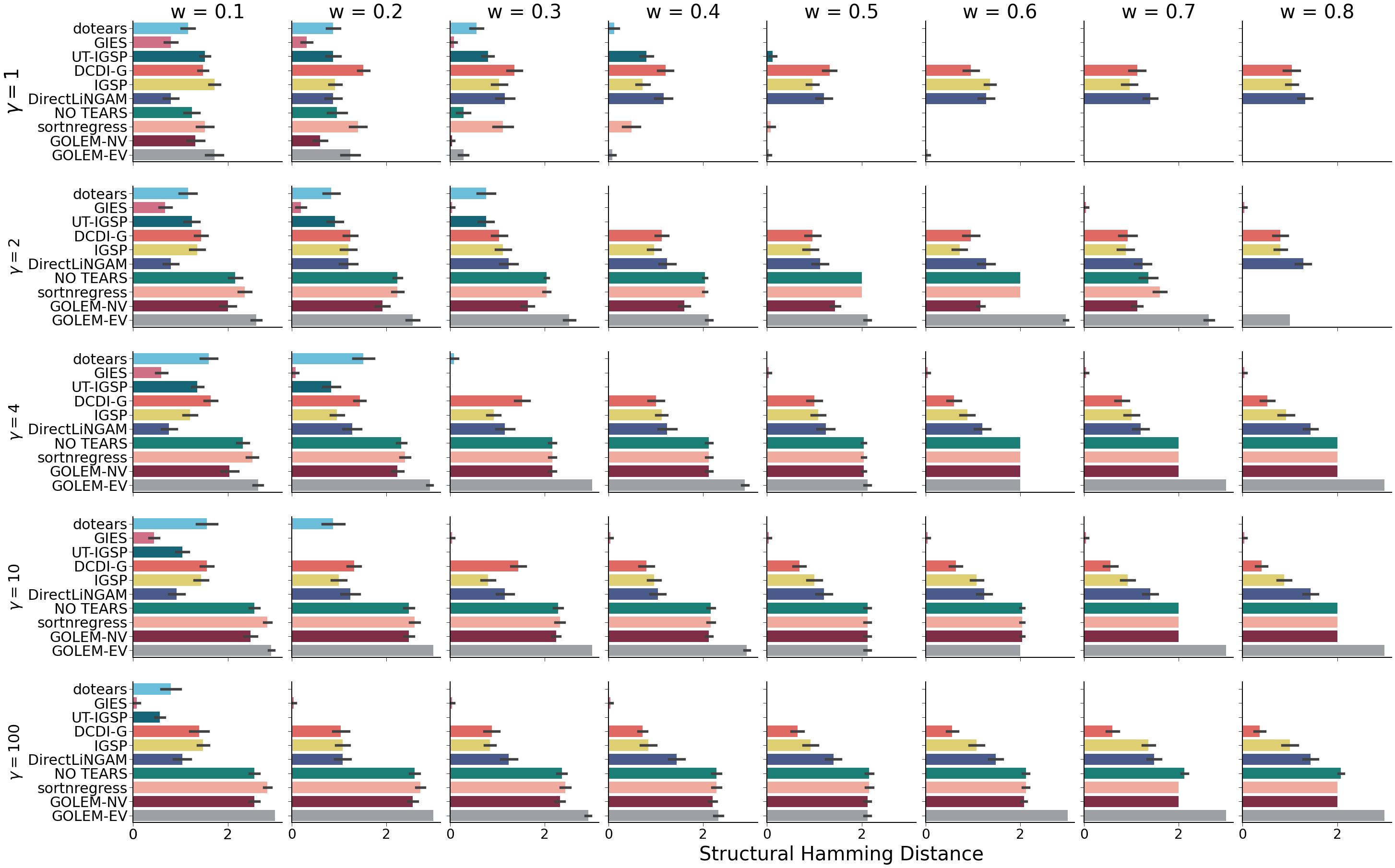
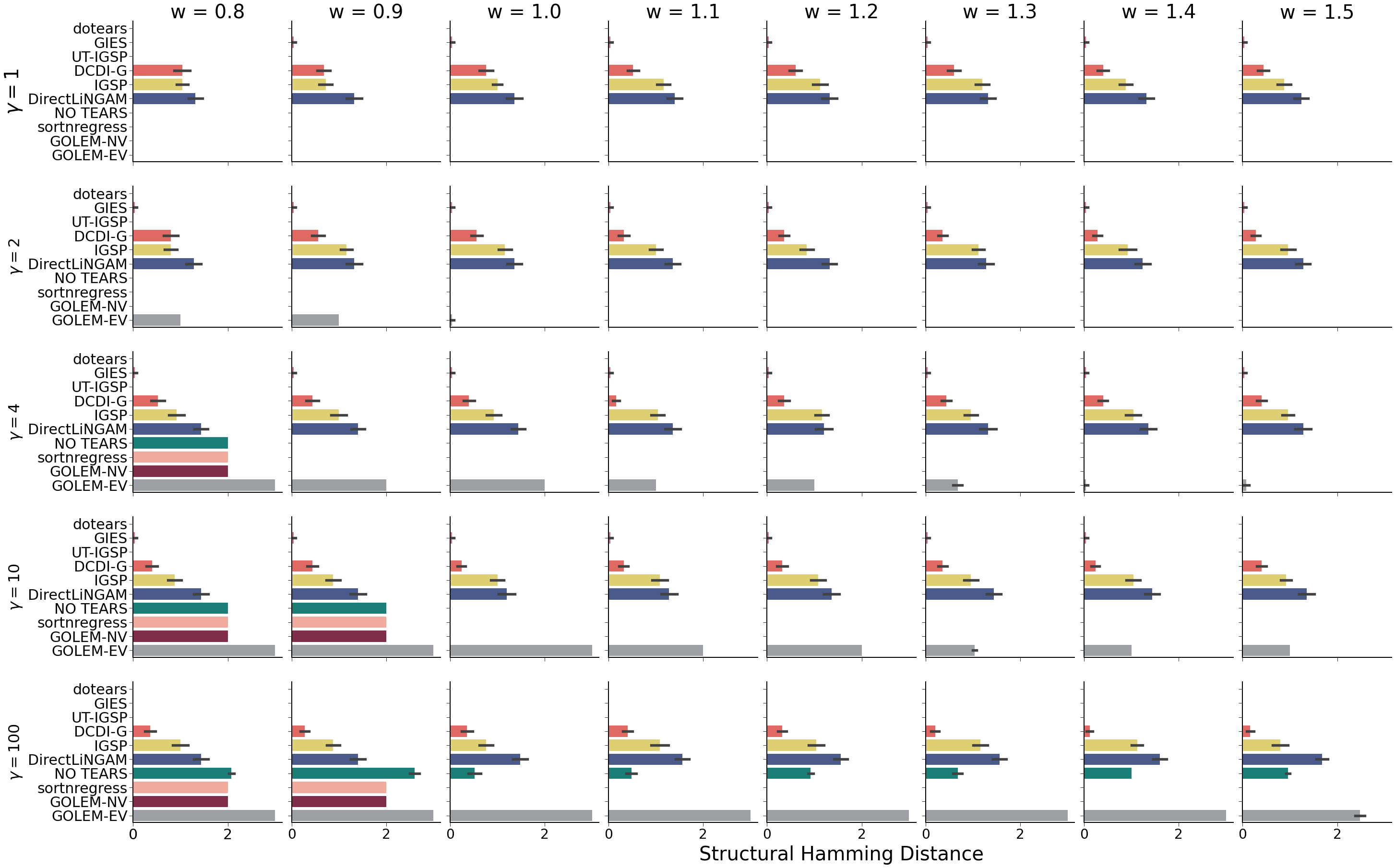
In the two node case, we let $\Omega_{0}=\begin{pmatrix}\gamma&0\\ 0&1\end{pmatrix}$ and $W_{0}=\begin{pmatrix}0&w\\ 0&0\end{pmatrix}$. For observational data, we draw Gaussian data under the SEM in Eq. 3. This data is also used in Figure 2. For the interventional methods, we draw Gaussian data under the system of observational and interventional SEMs in Supplementary Material 7.4. For each set of parameters $w,\gamma$, we draw 25 simulations of observational and interventional data, with sample size $n=(p+1)*1000=3000$ each. For observational data, this represents $3000$ observations from the observational system; for interventional data, this represents $1000$ observations from each system $k=0,1,2$. To isolate the behavior of the loss, we remove regularization where appropriate. Figure 3 shows the Structural Hamming Distance (SHD) between the true DAG $W_{0}$ and the inferred DAG for each method, for selected $w,\gamma$. SHD is defined as the number of edge insertions, deletions, and reversals required to transform one DAG to another. Full simulation details and results are given in Supplementary Material 7.4.

Refer to caption
Figure 3: Methodological comparison on simulated data for $w=0.3,0.5,0.7,0.8,1.0$ and $\gamma=1,2,100$. We generate Gaussian data from the structure $X_{1}\overset{w}{\rightarrow}X_{2}$, where $\sigma_{1}^{2}=\gamma\sigma_{2}^{2}$. For each pair $w,\gamma$, we draw 25 simulations at a sample size of $n=(p+1)*1000=3000$; for interventional methods, $n_{k}=1000$ observations were drawn for each intervention $k$. Methods are compared using Structural Hamming Distance (SHD) between the inferred DAG and the ground-truth DAG (lower is better). Black bars represent standard errors; some standard errors are too small to see.

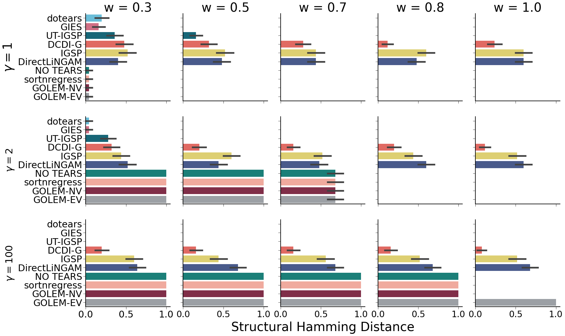
In Figure 3, GOLEM-NV is deterministic in $w,\gamma$, and correct only on varsortable pairs. However, the loss of GOLEM-NV is not least squares, and in fact provides a conditional estimate $\Omega_{0}\>|\>W$ using the residuals of $X-XW$ [12, 21]. This suggests that dependence on $\Omega_{0}$ generalizes beyond the least squares loss, and further that conditional estimation of $\Omega_{0}$ is insufficient for structure estimation. NO TEARS and GOLEM-NV perform identically in Figure 3, but become distinct deterministic functions of $w,\gamma$ in three node simulations (see Supplementary Material 7.5).

dotears is the only tested continuous optimization framework whose performance is independent of $\gamma$ (equivalently, $\Omega_{0}$). Under this simulation model, marginal estimation of $\Omega_{0}$ is thus sufficient to infer structure. dotears is one of only three structure learning methods (dotears, GIES, and UT-IGSP) to reliably estimate structure across $w,\gamma$. All three use interventional data, but IGSP and DCDI-G show that using interventional data is not sufficient for correct structure estimation.

5.2 Large random graph simulations

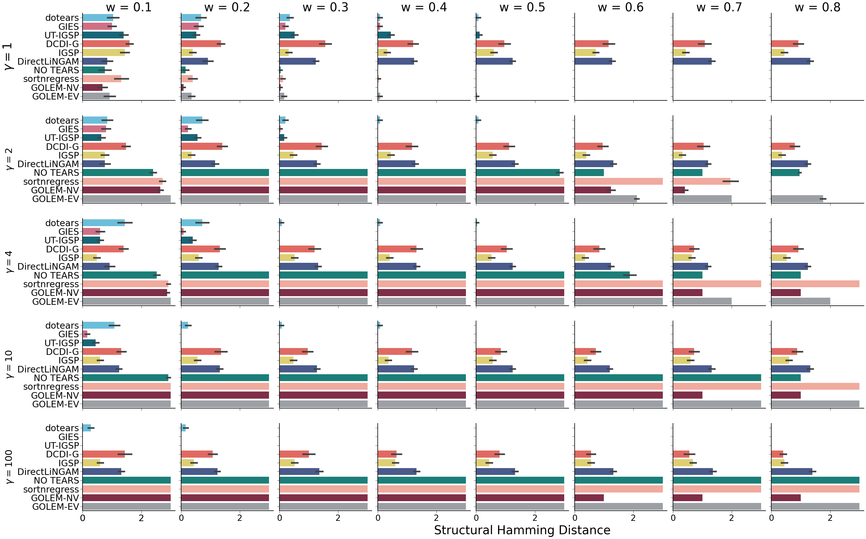
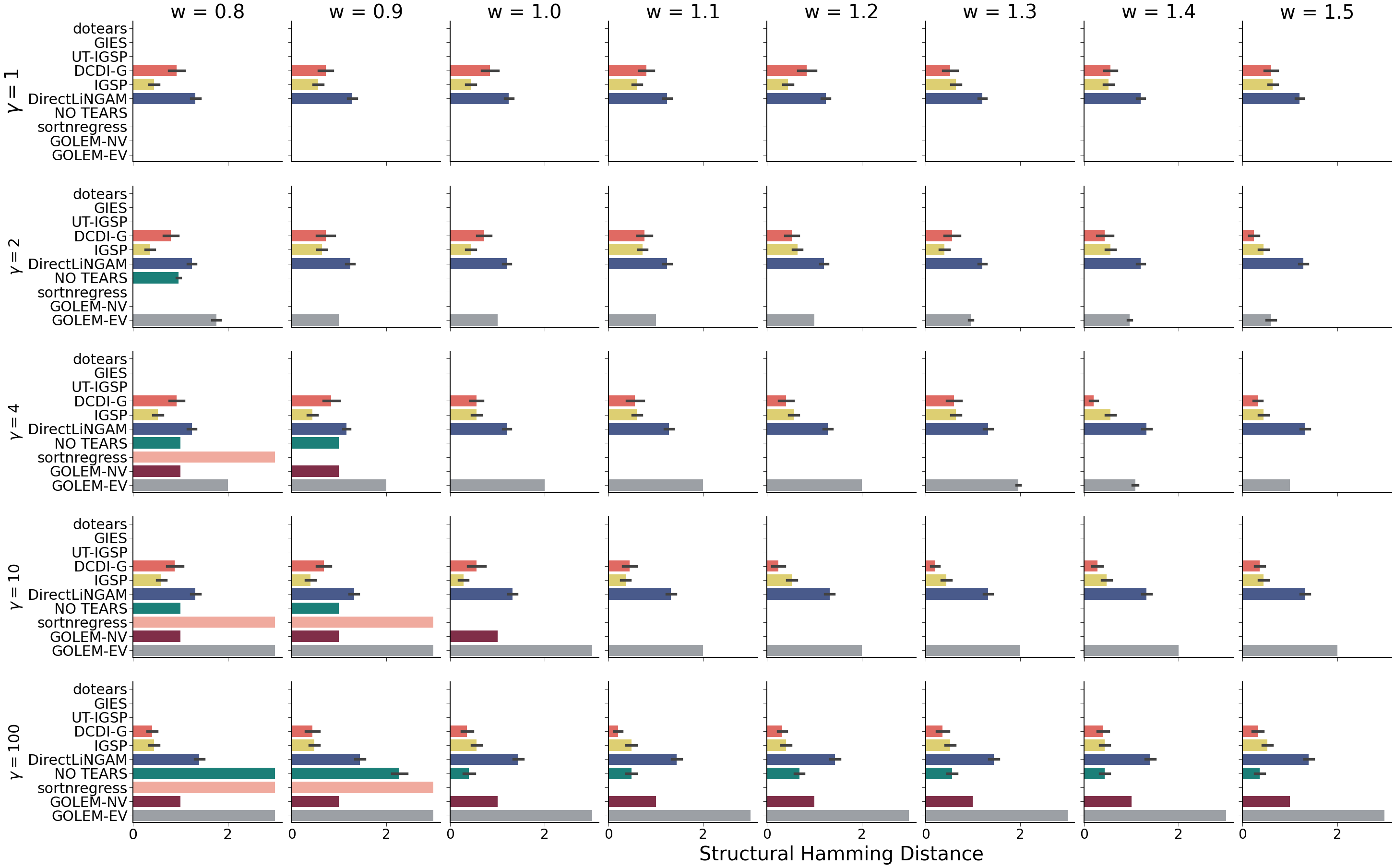
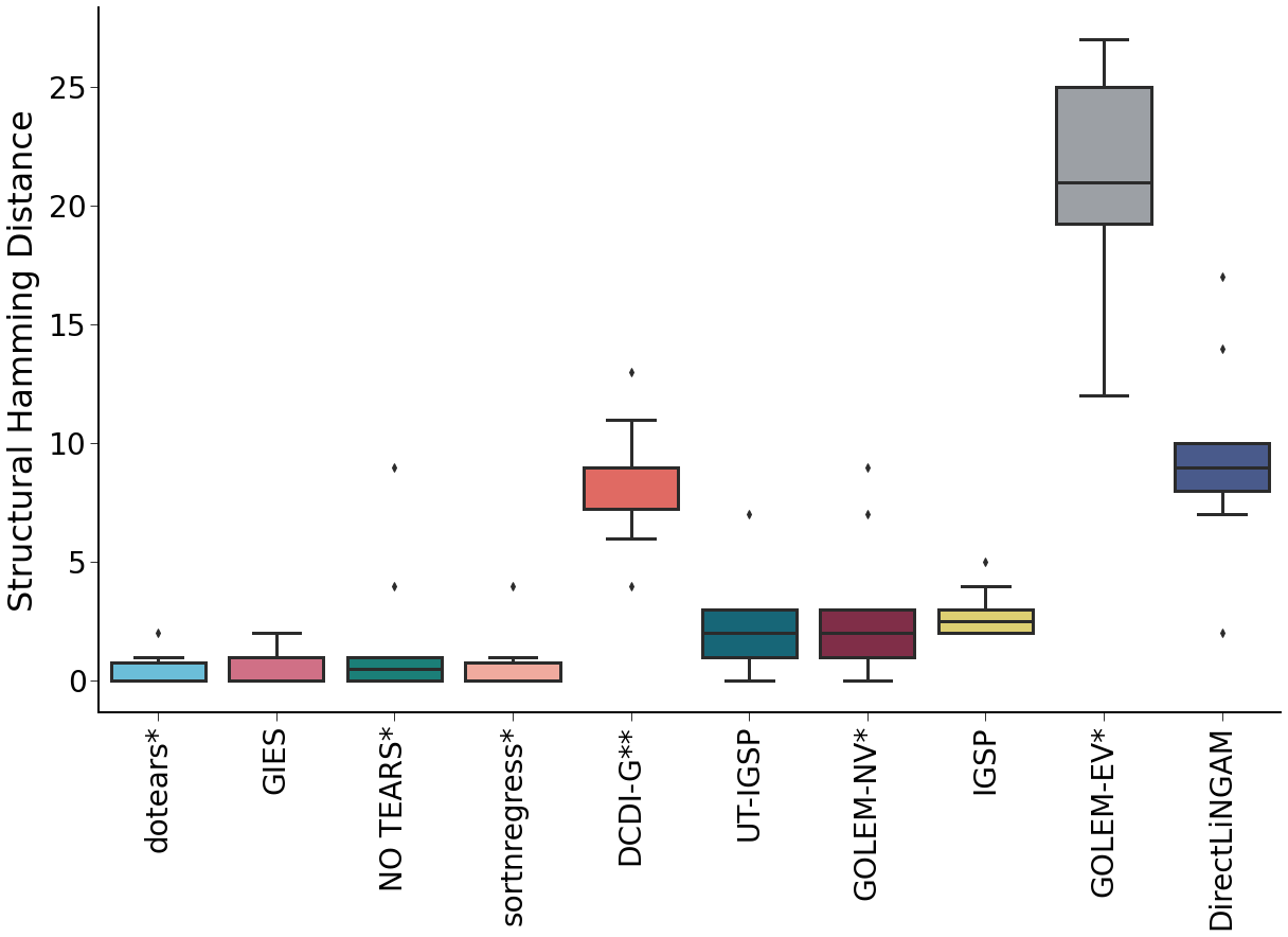
dotears outperforms all tested state of the art methods on synthetic data simulated from random networks with $p=50$. Structures are drawn from Erdős-Rényi (ER) and Scale-Free (SF) DAGs [27, 28]. We simulate under four possible parameterizations, which represent two parameterizations of edge density crossed with two parameterizations of edge weights: $\{\text{Low Density, High Density}\}\times\{\text{Weak Effects, Strong Effects}\}$. Observational and interventional data have sample size $n=(p+1)\times 100=5100$, matched as in Section 5.1. Methods performed under 5-fold cross-validation are denoted by *, i.e. dotears*. For non-binary methods, edge weights are thresholded for evaluation of SHD. Methods are robust to threshold choice (Supplementary Material 7.6.3) [11]. For simulation, cross-validation, and thresholding details, see Supplementary Material 7.6.1; for runtime and memory usage, see Supplementary Material 7.6.2.

Refer to caption
Figure 4: Relative performance (higher is better) to dotears across simulations for $p=50$. Relative performance is defined as $\frac{A-B}{A+1}$ over one simulation draw, where $A$ is the Structural Hamming Distance of dotears and $B$ is the Structural Hamming Distance of the compared method. Grey dashed line at 0 represents the baseline dotears performance. Methods are sorted, left to right, by average performance.
Refer to caption
Figure 5: Comparison of method performance on large random graphs ($p$ = 50) using Structural Hamming Distance (lower is better). Each row represents simulations with Erdős-Rényi or Scale Free topologies, respectively. Each column represents a different parameterization of edge density and edge weights, ordered in terms of increasing difficulty. For details, see Supplementary Material 7.6.1. 100 simulations were drawn for each parameterization with sample size $(p+1)*100=5100$, and * indicates cross-validated methods. Methods are sorted, left to right, by average performance.

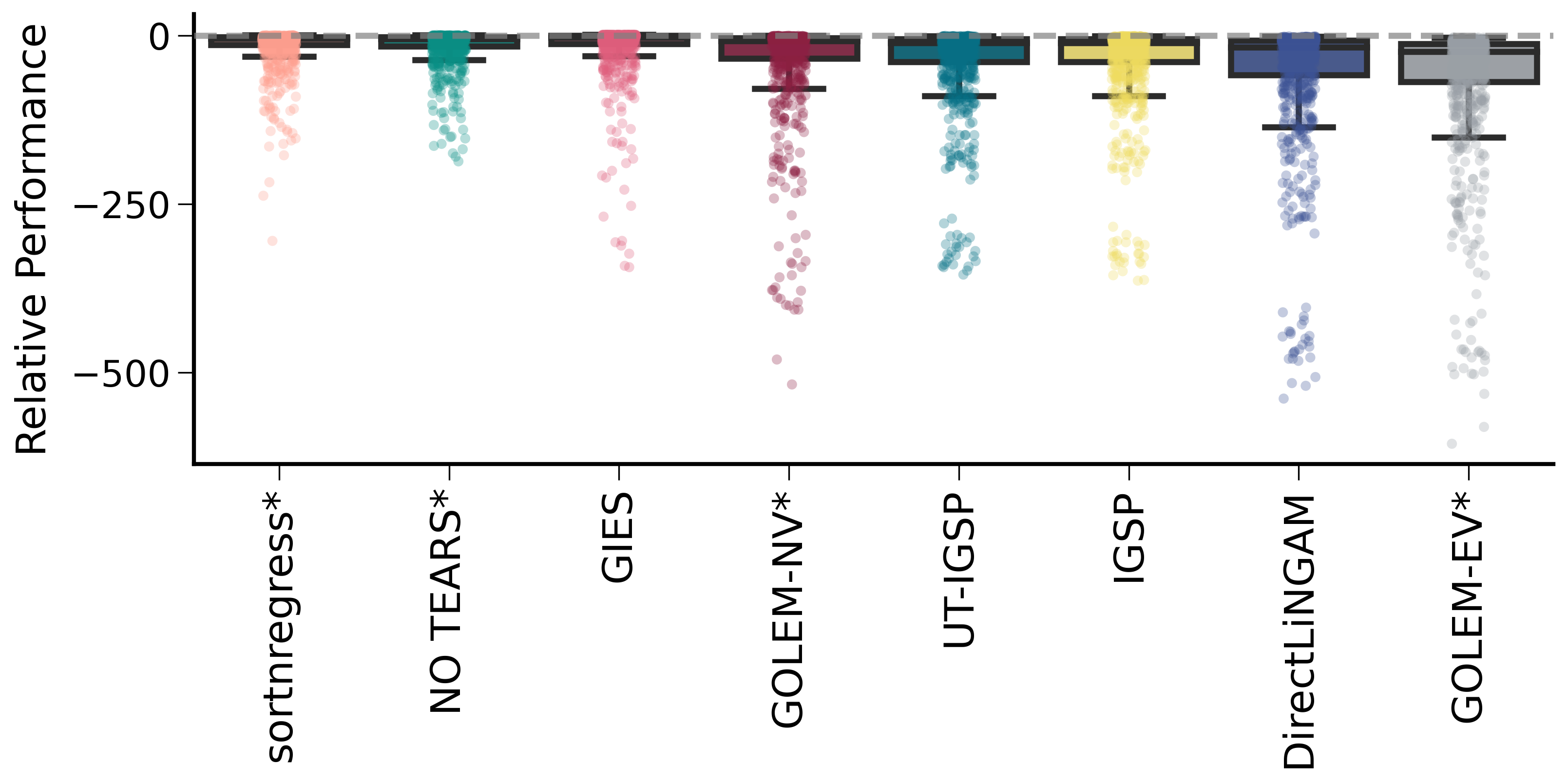
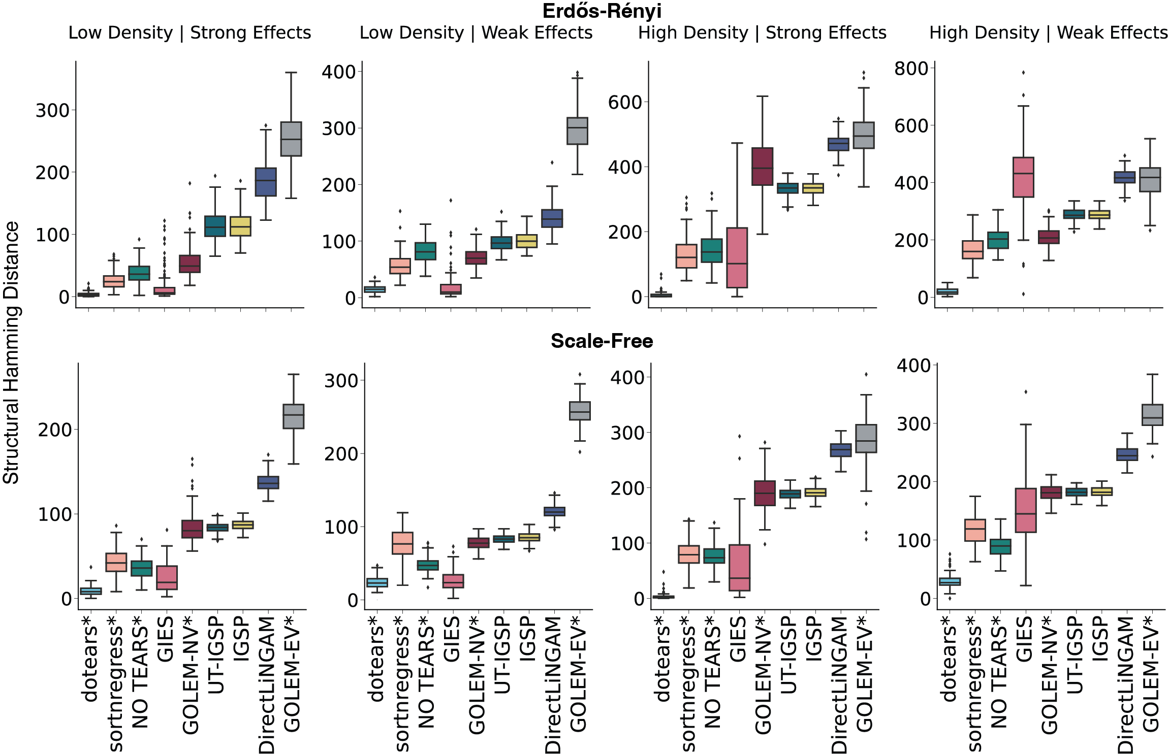
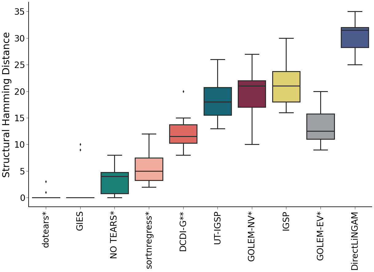
Averaged across parameterizations, all tested methods have greater SHD than dotears (Figure 4). Further, the distribution of SHD of all tested methods are significantly different from dotears under a Mann-Whitney U test (Supplementary Material 7.6.4). Averaged across parameter sets, sortnregress and NO TEARS were the second and third best performing methods after dotears, while the strongest performing interventional method was only 4th (GIES). dotears outperforms all other tested methods in terms of both structural recovery (SHD, Figure 5) and edge weight recovery ($\ell_{1}$ distance, Supplementary Figure 12). The sole exception is “Low Density" and “Weak Effects", where GIES outperforms dotears in median SHD (but not mean). However, GIES performs substantially worse in “High Density" simulations, which we hypothesize is due to the greedy nature of GIES.

For DCDI-G, memory usage issues were prohibitive for cross-validated runs on simulations with $p=50$. We ran DCDI-G in a limited number of smaller simulations ($p=10$), under a cross-validation procedure favorable to DCDI-G. In these simulations, DCDI-G is outperformed by dotears, GIES, NO TEARS, and sortnregress (in order). Full results are available in Supplementary Material 7.7.

6 Discussion

Our work demonstrates that inferences of many previous methods for Causal DAG inference are sensitive to exogenous variance structure. In response, we present dotears, a structure learning framework that estimates leverages interventional data to estimate exogenous variance structure and subsequently leverages observational and interventional data to learn the underlying causal graph. We verify that dotears is robust to exogenous variance structure, prove that its loss function provides consistent DAG estimation, and show that dotears outperforms all tested state-of-the-art methods in varied simulations on random graphs. In particular, since dotears extends NO TEARS, its substantial performance gain in simulations demonstrates the utility of our contributions.

To correct for exogenous variance structure, we make two key observations on the linear Structural Equation Model: 1.) a hard intervention creates a source node in the interventional system, and 2.) the marginal variance of a source node is equal to its exogenous variance. These observations are sufficient for estimation of exogenous variance under mild assumptions.

We caution that dotears is a nonconvex optimization problem, and is not guaranteed to arrive at a global minimum despite the consistency properties of its loss. Further, dotears is likely sensitive to violations of Assumption 1, which assumes that upstream variance is completely removed under intervention. We encourage future investigations to examine if relaxations of these assumptions provide consistent DAG estimation. Despite these limitations, dotears improves upon previous structure learning frameworks by combining robust, consistent structure estimation with a scalable optimization framework.

References

  • [1] Karen Sachs, Omar Perez, Dana Pe’er, Douglas A Lauffenburger, and Garry P Nolan. Causal protein-signaling networks derived from multiparameter single-cell data. Science, 308(5721):523–529, 2005.
  • [2] Bin Zhang, Chris Gaiteri, Liviu-Gabriel Bodea, Zhi Wang, Joshua McElwee, Alexei A Podtelezhnikov, Chunsheng Zhang, Tao Xie, Linh Tran, Radu Dobrin, et al. Integrated systems approach identifies genetic nodes and networks in late-onset alzheimer’s disease. Cell, 153(3):707–720, 2013.
  • [3] Andrew D Sanford and Imad A Moosa. A bayesian network structure for operational risk modelling in structured finance operations. Journal of the Operational Research Society, 63:431–444, 2012.
  • [4] Thomas Verma and Judea Pearl. On equivalence of causal models. In Proceedings of the Sixth Conference Annual Conference on Uncertainty in Artificial Intelligence (UAI-90), pages 220–227, 1990.
  • [5] Alain Hauser and Peter Bühlmann. Characterization and greedy learning of interventional markov equivalence classes of directed acyclic graphs. The Journal of Machine Learning Research, 13(1):2409–2464, 2012.
  • [6] Chandler Squires and Caroline Uhler. Causal structure learning: a combinatorial perspective. Foundations of Computational Mathematics, pages 1–35, 2022.
  • [7] Ali Shojaie and George Michailidis. Penalized likelihood methods for estimation of sparse high-dimensional directed acyclic graphs. Biometrika, 97(3):519–538, 2010.
  • [8] David Maxwell Chickering. Learning bayesian networks is np-complete. Learning from data: Artificial intelligence and statistics V, pages 121–130, 1996.
  • [9] Max Chickering, David Heckerman, and Chris Meek. Large-sample learning of bayesian networks is np-hard. Journal of Machine Learning Research, 5:1287–1330, 2004.
  • [10] Xun Zheng, Bryon Aragam, Pradeep K Ravikumar, and Eric P Xing. Dags with no tears: Continuous optimization for structure learning. Advances in neural information processing systems, 31, 2018.
  • [11] Alexander Reisach, Christof Seiler, and Sebastian Weichwald. Beware of the simulated dag! causal discovery benchmarks may be easy to game. Advances in Neural Information Processing Systems, 34:27772–27784, 2021.
  • [12] Marcus Kaiser and Maksim Sipos. Unsuitability of notears for causal graph discovery when dealing with dimensional quantities. Neural Processing Letters, 54(3):1587–1595, 2022.
  • [13] Atray Dixit, Oren Parnas, Biyu Li, Jenny Chen, Charles P Fulco, Livnat Jerby-Arnon, Nemanja D Marjanovic, Danielle Dionne, Tyler Burks, Raktima Raychowdhury, et al. Perturb-seq: dissecting molecular circuits with scalable single-cell rna profiling of pooled genetic screens. cell, 167(7):1853–1866, 2016.
  • [14] Joseph M Replogle, Reuben A Saunders, Angela N Pogson, Jeffrey A Hussmann, Alexander Lenail, Alina Guna, Lauren Mascibroda, Eric J Wagner, Karen Adelman, Gila Lithwick-Yanai, et al. Mapping information-rich genotype-phenotype landscapes with genome-scale perturb-seq. Cell, 185(14):2559–2575, 2022.
  • [15] Thomas M Norman, Max A Horlbeck, Joseph M Replogle, Alex Y Ge, Albert Xu, Marco Jost, Luke A Gilbert, and Jonathan S Weissman. Exploring genetic interaction manifolds constructed from rich single-cell phenotypes. Science, 365(6455):786–793, 2019.
  • [16] Po-Ling Loh and Peter Bühlmann. High-dimensional learning of linear causal networks via inverse covariance estimation. The Journal of Machine Learning Research, 15(1):3065–3105, 2014.
  • [17] Jonas Peters and Peter Bühlmann. Identifiability of gaussian structural equation models with equal error variances. Biometrika, 101(1):219–228, 2014.
  • [18] Wenyu Chen, Mathias Drton, and Y Samuel Wang. On causal discovery with an equal-variance assumption. Biometrika, 106(4):973–980, 2019.
  • [19] Frederick Eberhardt and Richard Scheines. Interventions and causal inference. Philosophy of Science, 74(5):981–995, 2007.
  • [20] Judea Pearl. Causality. Cambridge university press, 2009.
  • [21] Ignavier Ng, AmirEmad Ghassami, and Kun Zhang. On the role of sparsity and dag constraints for learning linear dags. Advances in Neural Information Processing Systems, 33:17943–17954, 2020.
  • [22] Karren Yang, Abigail Katcoff, and Caroline Uhler. Characterizing and learning equivalence classes of causal dags under interventions. In International Conference on Machine Learning, pages 5541–5550. PMLR, 2018.
  • [23] Yuhao Wang, Liam Solus, Karren Yang, and Caroline Uhler. Permutation-based causal inference algorithms with interventions. Advances in Neural Information Processing Systems, 30, 2017.
  • [24] Chandler Squires, Yuhao Wang, and Caroline Uhler. Permutation-based causal structure learning with unknown intervention targets. In Conference on Uncertainty in Artificial Intelligence, pages 1039–1048. PMLR, 2020.
  • [25] Philippe Brouillard, Sébastien Lachapelle, Alexandre Lacoste, Simon Lacoste-Julien, and Alexandre Drouin. Differentiable causal discovery from interventional data. Advances in Neural Information Processing Systems, 33:21865–21877, 2020.
  • [26] Shohei Shimizu, Takanori Inazumi, Yasuhiro Sogawa, Aapo Hyvarinen, Yoshinobu Kawahara, Takashi Washio, Patrik O Hoyer, Kenneth Bollen, and Patrik Hoyer. Directlingam: A direct method for learning a linear non-gaussian structural equation model. Journal of Machine Learning Research-JMLR, 12(Apr):1225–1248, 2011.
  • [27] Paul Erdős, Alfréd Rényi, et al. On the evolution of random graphs. Publ. Math. Inst. Hung. Acad. Sci, 5(1):17–60, 1960.
  • [28] Albert-László Barabási and Réka Albert. Emergence of scaling in random networks. science, 286(5439):509–512, 1999.
  • [29] Yuhao Wang, Chandler Squires, Anastasiya Belyaeva, and Caroline Uhler. Direct estimation of differences in causal graphs. Advances in neural information processing systems, 31, 2018.
  • [30] Johannes Köster and Sven Rahmann. Snakemake—a scalable bioinformatics workflow engine. Bioinformatics, 28(19):2520–2522, 2012.
  • [31] Gabor Csardi and Tamas Nepusz. The igraph software package for complex network research. InterJournal, Complex Systems:1695, 2006.

7 Supplementary Material

7.1 Proofs for varsortability

7.1.1 Proof of Lemma 1

Proof.

Under the generative SEM in Eq. 3, we have

$$\begin{aligned} \text{Var}\left(X_{1}\right)&=\sigma_{1}^{2}\\ \text{Var}\left(X_{2}\right)&=w^{2}\sigma_{1}^{2}+\sigma_{2}^{2}\end{aligned}.$$ (9)

The system is therefore varsortable if and only if $w^{2}\sigma_{1}^{2}+\sigma_{2}^{2}\geq\sigma_{1}^{2}$. Using the substitution $\sigma_{1}^{2}=\gamma\sigma_{2}^{2}$, we obtain

$\displaystyle w^{2}\sigma_{1}^{2}+\sigma_{2}^{2}$ $\displaystyle\geq\sigma_{1}^{2}$ (10)
$\displaystyle w^{2}\gamma\sigma_{2}^{2}+\sigma_{2}^{2}$ $\displaystyle\geq\gamma\sigma_{2}^{2}$
$\displaystyle w^{2}\gamma+1$ $\displaystyle\geq\gamma$
$\displaystyle|w|$ $\displaystyle\geq\sqrt{1-\frac{1}{\gamma}}$

7.1.2 Proof of Theorem 1

Proof.

From Eq. 5, we can calculate both $\mathbb{E}\ell\left(W_{0},\boldsymbol{X}\right)$ and $\mathbb{E}\ell\left(W_{\delta},\boldsymbol{X}\right)$ component-wise. Under $W_{0}$ we obtain component-wise

$\displaystyle\left({X}-{X}W_{0}\right)_{1}$ $\displaystyle={X_{1}}$ (11)
$\displaystyle={\epsilon_{1}}$ by Eq. 3
$\displaystyle\left({X}-{X}W_{0}\right)_{2}$ $\displaystyle={X_{2}}-w{X_{1}}$
$\displaystyle={\epsilon_{2}}$ by Eq. 3

As a result,

$\displaystyle\mathbb{E}\ell\left(W_{0},\boldsymbol{X}\right)$ $\displaystyle=\frac{1}{2n_{0}}\sum_{i=1}^{p}\mathbb{E}\left|\left|\left({\boldsymbol{X}}-{\boldsymbol{X}}W_{0}\right)_{i}\right|\right|_{F}^{2}$ (12)
$\displaystyle=\frac{1}{2n_{0}}\left(\mathbb{E}\left(\left|\left|{\boldsymbol{\epsilon}_{1}}\right|\right|_{F}^{2}\right)+\mathbb{E}\left(\left|\left|\boldsymbol{\epsilon}_{2}\right|\right|_{F}^{2}\right)\right)$
$\displaystyle=\frac{1}{2}\left(\sigma_{1}^{2}+\sigma_{2}^{2}\right)$

Here we note that the expected loss under the generative DAG is $\mathbb{E}\ell\left(W_{0},\boldsymbol{X}\right)=\frac{1}{2}\sum_{i=1}^{p}\text{Var}\left({\epsilon_{i}}\right)$.

Similarly, under $W_{\delta}$ we have

$\displaystyle\left(X-XW_{\delta}\right)_{1}$ $\displaystyle=X_{1}-\delta X_{2}$ (13)
$\displaystyle=\epsilon_{1}-\delta\left(w\epsilon_{1}+\epsilon_{2}\right)$ by Eq. 3
$\displaystyle=(1-\delta w)\epsilon_{1}-\delta\epsilon_{2}$
$\displaystyle\left(X-XW_{\delta}\right)_{2}$ $\displaystyle=X_{2}$
$\displaystyle=w\epsilon_{1}+\epsilon_{2}$ by Eq. 3

and therefore

$$\mathbb{E}\ell\left(W_{\delta},\boldsymbol{X}\right)=\frac{1}{2}\left(\sigma_{1}^{2}\left(w^{2}+\left(1-\delta w\right)^{2}\right)+\sigma_{2}^{2}\left(1+\delta^{2}\right)\right).$$ (14)

We can now ask when $\mathbb{E}\ell\left(W_{\delta},\boldsymbol{X}\right)\leq\mathbb{E}\ell\left(W_{0},\boldsymbol{X}\right)$, or equivalently,

$\displaystyle\sigma_{1}^{2}\left(w^{2}+\left(1-\delta w\right)^{2}\right)+\sigma_{2}^{2}\left(1+\delta^{2}\right)$ $\displaystyle\leq\sigma_{1}^{2}+\sigma_{2}^{2}$ (15)
$\displaystyle(\text{by }\sigma_{1}^{2}=\gamma\sigma_{2}^{2})\iff$ $\displaystyle\gamma\sigma_{2}^{2}\left(w^{2}+\left(1-\delta w\right)^{2}\right)+\sigma_{2}^{2}\left(1+\delta^{2}\right)$ $\displaystyle\leq\gamma\sigma_{2}^{2}+\sigma_{2}^{2}$
$\displaystyle\iff$ $\displaystyle\gamma\left(w^{2}+1-2\delta w+\delta^{2}w^{2}\right)+1+\delta^{2}$ $\displaystyle\leq\gamma+1$
$\displaystyle\iff$ $\displaystyle\gamma\left(w^{2}-2\delta w+\delta^{2}w^{2}\right)+\delta^{2}$ $\displaystyle\leq 0$
$\displaystyle\iff$ $\displaystyle\delta^{2}\left(1+\gamma w^{2}\right)-\delta\left(2\gamma w\right)+\gamma w^{2}$ $\displaystyle\leq 0$

The inequality becomes a quadratic in $\delta$, which when solved gives us roots at

$\displaystyle\delta$ $\displaystyle=\frac{2\gamma w\pm\sqrt{(-2\gamma w)^{2}-4\left(1+\gamma w^{2}\right)\left(\gamma w^{2}\right)}}{2\left(1+\gamma w^{2}\right)}$ (16)
$\displaystyle=\frac{2\gamma w\pm 2\gamma w\sqrt{1-\frac{1}{\gamma}\left(1+\gamma w^{2}\right)}}{2\left(1+\gamma w^{2}\right)}$
$\displaystyle=\frac{\gamma w\left(1\pm\sqrt{1-w^{2}-\frac{1}{\gamma}}\right)}{1+\gamma w^{2}}.$

Note that for the quadratic in Eq. 15, $\gamma w^{2}\geq 0$. Then $\exists\delta$ such that $\mathbb{E}\ell\left(W_{\delta},\boldsymbol{X}\right)\leq\mathbb{E}\ell\left(W_{0},\boldsymbol{X}\right)$ when the term in the root exists in Eq. 16. Equivalently, we can say that $\mathbb{E}\ell\left(W_{0},\boldsymbol{X}\right)\leq\mathbb{E}\ell\left(W_{\delta},\boldsymbol{X}\right)$ is guaranteed for all $\delta$ if and only if

$$|w|\geq\sqrt{1-\frac{1}{\gamma}}.$$ (17)

7.2 Proof of Consistency

For a diagonal matrix $\Omega$, define

$\displaystyle\mathcal{L}_{\Omega}\left(W^{(k)},\boldsymbol{X}^{(k)}\right)$ $\displaystyle\coloneqq\frac{1}{n_{k}}\left|\left|\left(\boldsymbol{X}^{(k)}-\boldsymbol{X}^{(k)}W^{(k)}\right)\Omega^{-\frac{1}{2}}\right|\right|_{F}^{2}$ (18)
$\displaystyle=\frac{1}{n_{k}}\sum_{j=1}^{p}\frac{1}{\Omega_{jj}}\left|\left|\left(\boldsymbol{X}^{(k)}-\boldsymbol{X}^{(k)}W^{(k)}\right)_{j}\right|\right|_{F}^{2},$

where $\Omega_{jj}$ is the $j,j$th entry of $\Omega$. Further, recall the definition

$$\Omega_{0}^{(k)}\coloneqq\text{Cov}\left(\epsilon^{(k)}\right).$$ (19)

Denote convergence in probability by $\overset{p}{\rightarrow}.$

Lemma 2.

For any intervention $k$,

$$\mathcal{L}_{{\Omega}_{0}}\left(W^{(k)},\boldsymbol{X}^{(k)}\right)=\mathcal{L}_{\Omega_{0}^{(k)}}\left(W^{(k)},\boldsymbol{X}^{(k)}\right)+\mathcal{O}_{W}(1)$$

For the proof, see Supplementary Material 7.2.1.

Corollary 2.
$$\arg\min_{W}\mathcal{L}_{\Omega_{0}}\left(W^{(k)},\boldsymbol{X}^{(k)}\right)=\arg\min_{W}\mathcal{L}_{\Omega_{0}^{(k)}}\left(W^{(k)},\boldsymbol{X}^{(k)}\right)$$

For any intervention $k$ and any $\alpha$, Lemma 2 and Corollary 2 show that true exogenous variance structure $\Omega_{0}=\alpha^{2}\mathbb{E}\hat{\Omega}_{0}$ is sufficient for structure recovery. Results from Loh and Buhlmann (2014) are then sufficient to establish consistency of the estimator $\operatorname*{arg\,min}_{W}\mathcal{L}_{\Omega_{0}}\left(W^{(k)},X^{(k)}\right)$. We wish to show consistency of $\operatorname*{arg\,min}_{W}\mathcal{L}_{\hat{\Omega}_{0}}\left(W^{(k)},\boldsymbol{X}^{(k)}\right)$, where we have an estimated $\hat{\Omega}_{0}$ rather than $\Omega_{0}$.

For simplicity, in the following we assume $\alpha=1$ without loss of generality, which is justified by Corollary 2 and Lemma 2. Note then that $\Omega_{0}=\Omega_{0}^{(k)}$, which allows us to drop the (k) notation.

Remark 1.

For consistency under an estimated $\hat{\Omega}_{0}$, we have two cases: the observational case $k=0$ and the interventional case $k\neq 0$. The observational case is simplest - in particular, when $k=0$, $\hat{\Omega}_{0}$ is independent of $\boldsymbol{X}^{(0)}$, and we may therefore freely estimate $W_{0}^{(0)}$ from $\mathcal{L}_{\hat{\Omega}_{0}}\left(W^{(0)},\boldsymbol{X}^{(0)}\right)$. When $k\neq 0$, we can assume independence of $\hat{\Omega}_{0}$ and $\boldsymbol{X}^{(k)}$ under a data splitting framework, where some fraction of our $n_{k}$ samples are reserved for estimation of $\hat{\sigma}_{k}^{2}$, and the remaining samples are given in $\boldsymbol{X}^{(k)}$.

Assumption 5.

Let

$$\hat{\sigma}_{k}^{2}\coloneqq\left(\hat{\Omega}_{0}\right)_{kk}.$$ (20)

Then

$$\hat{\sigma}_{k}^{2}\mathchoice{\mathrel{\hbox to0.0pt{$\displaystyle\perp$\hss}\mkern 2.0mu{\displaystyle\perp}}}{\mathrel{\hbox to0.0pt{$\textstyle\perp$\hss}\mkern 2.0mu{\textstyle\perp}}}{\mathrel{\hbox to0.0pt{$\scriptstyle\perp$\hss}\mkern 2.0mu{\scriptstyle\perp}}}{\mathrel{\hbox to0.0pt{$\scriptscriptstyle\perp$\hss}\mkern 2.0mu{\scriptscriptstyle\perp}}}\boldsymbol{X}^{(k)}_{k}.$$ (21)

However, in the presented applications we use the full $n_{k}$ samples of $\boldsymbol{X}_{k}^{(k)}$ for both estimates.

Note that we abuse notation to write $\boldsymbol{X}^{(k)}$ as the set of samples used to estimate $\hat{W}_{0}^{(k)}$ given $\hat{\Omega}_{0}$. Further, for convenience we abuse notation to write $n_{k}$ as the sample size of $\boldsymbol{X}^{(k)}$ AND the sample size of $\hat{\sigma}_{k}^{2}$, since the respective sample sizes are equal to $n_{k}$ up to a multiplicative constant which can be ignored as $n_{k}\to\infty$.

We further define

$$\mathbb{E}\mathcal{L}_{\Omega}\left(W^{(k)},\boldsymbol{X}^{(k)}\right)\coloneqq\frac{1}{n_{k}}\sum_{j=1}^{p}\frac{1}{\Omega_{jj}}\mathbb{E}\left|\left|\left(\boldsymbol{X}^{(k)}-\boldsymbol{X}^{(k)}W^{(k)}\right)_{j}\right|\right|_{F}^{2}.$$ (22)

Here, we abuse notation to remove $\Omega_{jj}$ from the expectation. Moreover, for the random vector $X$ we write

$$\mathbb{E}\mathcal{L}_{\Omega}\left(W^{(k)},X^{(k)}\right)\coloneqq\sum_{j=1}^{p}\frac{1}{\Omega_{jj}}\mathbb{E}\left[\left(X^{(k)}-X^{(k)}W^{(k)}\right)_{j}^{2}\right],$$ (23)

and note that the two definitions are equivalent under expectation. Note further that

$$\text{score}_{\Omega}(W)\equiv\mathbb{E}\mathcal{L}_{\Omega}(W,X),$$ (24)

where score is defined in [16].

Remark 2.

Loh and Buhlmann differentiate between the weighted adjacency matrix $W$ and the binary DAG $G$. In particular, they define

$$\text{score}_{\Omega}\left(G,X\right)\coloneqq\min_{W\in\mathcal{U}_{G}}\left\{\text{score}_{\Omega}\left(W,X\right)\right\},$$ (25)

where $\mathcal{U}_{G}$ is the set of weighted adjacency matrices with support in $G$. However, for the true binary DAG $G_{0}$,

$$\text{score}_{\Omega}\left(G,X\right)=\text{score}_{\Omega}\left(G_{0},X\right)\quad\forall G\supseteq G_{0},$$ (26)

which leads to identifiability issues (see Lemma 6 and discussion of Lemma 19 [16]).

We define everything directly on the weighted adjacency matrix $W$, and ignore the binary DAG $G$. This discrepancy is essentially due to methodological differences. Loh and Buhlmann first find a superset of the binary structure $G_{0}$, and subsequently rely on sparse regression to recover edge weights [16]. However, dotears searches directly in the space of weighted adjacency matrices to find $W_{0}$. While the end result is similar, we use this remark to explain discrepancies in notation and proof structure for readers following with [16].

We start by restating results from [16]. Let $\Omega_{1}\in\mathbb{R}^{p\times p}$ an arbitrary diagonal weight matrix. Define

$$a_{\text{max}}\coloneqq\lambda_{\text{max}}\left(\Omega_{0}\Omega_{1}^{-1}\right)\quad\text{and}\quad a_{\text{min}}\coloneqq\lambda_{\text{min}}\left(\Omega_{0}\Omega_{1}^{-1}\right)$$ (27)

to be the maximum and minimum ratios between the corresponding diagonal entries of $\Omega_{0}$ and $\Omega_{1}$, and further define

$$\xi^{(k)}_{\Omega}\coloneqq\min_{\begin{subarray}{c}W\in\mathcal{D}\\ W\neq W_{0}\end{subarray}}\left\{\mathbb{E}\mathcal{L}_{\Omega}\left(W^{(k)},X^{(k)}\right)-\mathbb{E}\mathcal{L}_{\Omega}\left(W_{0}^{(k)},X^{(k)}\right)\right\}$$ (28)

to be the additive gap between the expected loss of the true weighted adjacency matrix $W_{0}$ and the expected loss of the next-best weighted adjacency matrix under an arbitrary diagonal matrix $\Omega$. Note that $\xi_{\Omega_{0}}>0$ (see Theorem 7 in [16]). Then we have the following theorem, whose proof is given in [16]:

Theorem 2.

Suppose

$$\frac{a_{\text{max}}}{a_{\text{min}}}\leq 1+\frac{\xi_{\Omega_{0}}^{(k)}}{p}.$$ (29)

Then $W_{0}^{(k)}\in\operatorname*{arg\,min}_{W\in\mathcal{D}}\left\{\mathbb{E}\mathcal{L}_{\Omega_{1}}\left(W,X^{(k)}\right)\right\}$. If Inequality 29 is strict, then $W_{0}^{(k)}$ is the unique minimizer of $\mathbb{E}\mathcal{L}_{\Omega_{1}}\left(W,X^{(k)}\right)$.

Theorem 3.

For any intervention $k$, as $n_{j}\to\infty$ for all $j=1,\dots,p$, with high probability $W_{0}^{(k)}$ is the unique minimizer of $\mathbb{E}\mathcal{L}_{\hat{\Omega}_{0}}\left(W^{(k)},X^{(k)}\right)$, and thus $\xi_{\hat{\Omega}_{0}}^{(k)}>0$.

For the proof, see Supplementary Material 7.2.2.

Lemma 3.

For any intervention $k$, suppose $X^{(k)}$ is a sub-Gaussian random vector with parameter $\sigma^{2}$. Then $X^{(k)}_{k}$ is a sub-Gaussian random variable with parameter $\sigma^{2}$, and for all $t\geq 0$, we have

$$\left|\frac{1}{\hat{\sigma}_{k}^{2}}-\frac{1}{\sigma_{k}^{2}}\right|\leq\frac{2\sigma^{2}}{\sigma_{k}^{2}}\cdot\max\{\delta,\delta^{2}\}$$ (30)

with probability at least $1-2\exp(-cn_{k}t^{2})$, where $\delta=c^{\prime}\sqrt{\frac{1}{n_{k}}}+c^{\prime\prime}t$ and

$$\frac{\sigma^{2}}{\sigma_{k}^{2}}\cdot\max\{\delta,\delta^{2}\}\leq\frac{1}{2}.$$ (31)
Proof.

Lemma 31 is a re-statement of Lemma 29 in [16] (Appendix E) for the degenerate case $p=1$. ∎

Following [16], we introduce the new notation $f^{(k)}_{\sigma_{j}}$. For a node $j$ and a set $S\subseteq\{1\dots p\}\backslash\{j\}$, define

$$f^{(k)}_{\sigma_{j}}(S)\coloneqq\frac{1}{\sigma_{j}^{2}}\mathbb{E}\left[\left(X^{(k)}_{j}-X^{(k)}_{S}w_{j}\right)^{2}\right],$$ (32)

where $X^{(k)}_{j}$ is the $j$th column vector of $X^{(k)}$, and $X^{(k)}_{S}w_{j}$ is the best linear predictor for $X^{(k)}_{j}$ regressed upon $X_{S}^{(k)}$. Similarly,

$$\hat{f}_{\sigma_{j}}^{(k)}(S)\coloneqq\frac{1}{\sigma_{j}^{2}}\frac{1}{n_{k}}\left|\left|\boldsymbol{X}^{(k)}_{j}-\boldsymbol{X}^{(k)}_{S}\hat{w}_{j}\right|\right|_{F}^{2},$$ (33)

where $\hat{w}_{j}$ is the ordinary least squares solution for linear regression of $\boldsymbol{X}^{(k)}_{j}$ upon $\boldsymbol{X}^{(k)}_{S}$, i.e.

$\displaystyle\hat{w}_{j}$ $\displaystyle\coloneqq\left(\left(\left(\boldsymbol{X}^{(k)}_{S}\right)^{\textrm{T}}\boldsymbol{X}^{(k)}_{S}\right)^{-1}\left(\boldsymbol{X}^{(k)}_{S}\right)^{\textrm{T}}\boldsymbol{X}^{(k)}_{j}\right)$ (34)
$\displaystyle=\left(\left(\left(\boldsymbol{X}^{(k)}_{S}\right)^{\textrm{T}}\boldsymbol{X}^{(k)}_{S}\right)^{-1}\left(\boldsymbol{X}^{(k)}_{S}\right)^{\textrm{T}}\left(\boldsymbol{X}^{(k)}_{S}w_{j}+\boldsymbol{e}^{(k)}_{j}\right)\right)$
$\displaystyle=w_{j}+\left(\left(\boldsymbol{X}^{(k)}_{S}\right)^{\textrm{T}}\boldsymbol{X}^{(k)}_{S}\right)^{-1}\left(\boldsymbol{X}^{(k)}_{S}\right)^{\textrm{T}}\boldsymbol{e}^{(k)}_{j},$

where note that

$$\boldsymbol{X}_{j}^{(k)}=\boldsymbol{X}_{S}^{(k)}w_{j}+\boldsymbol{e}^{(k)}_{j}.$$ (35)

Lastly, denote the vector $\ell_{2}$ norm as $\|\|\cdot\|\|_{2}$.

Loh and Buhlmann achieve a high-dimensional consistency result by first conditioning on the support of a sparse precision matrix $\Theta^{(k)}$, since the support of $\Theta^{(k)}\coloneqq\text{Cov}\left(X^{(k)}\right)^{-1}$ defines the moralized graph, an undirected graph obtained from a DAG by adding edges between all parents with a shared child node [16, 29]. Since the edge set of the moralized graph is a superset of the edge set of the true DAG, for a given node $j$ one may condition on the maximum size of the putative neighbor set, $N_{\Theta^{(k)}}(j)$. Indeed, in [16] Loh and Buhlmann restrict $|N_{\Theta^{(k)}}(j)|\leq d$ for all $j$, with the only restriction on $d$ being that $d\leq n$.

dotears does not condition on $\Theta^{(k)}$, and therefore does not condition on the moralized graph or $N_{\Theta}(j)$. To maintain the validity of our consistency proof, we let $d=p-1\leq n$. Under this restriction, we no longer have a high-dimensional result, but maintain consistency of the loss function of dotears for low dimensionality of $p$.

Assumption 6.

For all $k=0,\dots,p$, let $d=p-1\leq n_{k}$.

Lemma 4.

For any intervention $k$, suppose $X^{(k)}$ is sub-Gaussian with parameter $\sigma^{2}$. Then $\forall j\text{ and }S\subseteq\{1\dots p\}\backslash\{j\}$,

$$\sigma_{j}^{2}\left|\hat{f}^{(k)}_{\hat{\sigma}_{j}}(S)-\hat{f}^{(k)}_{\sigma_{j}}(S)\right|\leq\sigma^{2}\cdot\max\{\delta,\delta^{2}\}\cdot\frac{C}{n_{k}}\left|\left|\boldsymbol{e}^{(k)}_{j}\right|\right|_{2}^{2}$$ (36)

with probability $1-c_{1}\exp(-c_{2}\log p)$, where $\delta=c^{\prime}\sqrt{\frac{1}{n_{j}}}+c^{\prime\prime}\sqrt{\frac{\log p}{n_{j}}}$, if

$$\frac{\sigma^{2}}{\sigma_{j}^{2}}\cdot\delta\leq\frac{1}{2}.$$ (37)

For the proof, see Supplementary Material 7.2.3.

Lemma 5.

For any intervention $k$, suppose $X^{(k)}$ is sub-Gaussian with parameter $\sigma^{2}$. Then as $n_{i}\to\infty$ for all $i=1\dots p$, $\forall j\text{ and }S\subseteq\{1\dots p\}\backslash\{j\}$ it is true that

$$\left|\hat{f}^{(k)}_{\hat{\sigma}_{j}}(S)-f^{(k)}_{\sigma_{j}}(S)\right|\leq c_{0}\sigma^{4}\sqrt{\frac{\log p}{n_{j}}}+c_{1}\sigma^{2}\sqrt{\frac{\log p}{n_{k}}}+c_{2}\frac{p}{n_{k}}$$ (38)

with probability at least $1-c_{1}\exp(-c_{2}\log p)$.

For the proof, see Supplementary Material 7.2.4.

Theorem 4.

For any intervention $k$, suppose Inequality 38 holds, and suppose

$$\left(c_{0}\sigma^{4}\sqrt{\frac{\log p}{n_{j}}}+c_{1}\sigma^{2}\sqrt{\frac{\log p}{n_{k}}}+c_{2}\frac{p}{n_{k}}\right)\cdot\sum_{j=1}^{p}\frac{1}{\sigma_{j}^{2}}<\frac{\xi_{{\Omega}_{0}}^{(k)}}{2}.$$ (39)

Then

$$\mathcal{L}_{\hat{\Omega}_{0}}\left(W_{0}^{(k)},\boldsymbol{X}^{(k)}\right)<\mathcal{L}_{\hat{\Omega}_{0}}\left(W^{(k)},\boldsymbol{X}^{(k)}\right)\quad\forall W\in\mathcal{D},$$ (40)

and the estimator

$$\hat{W}^{(k)}\coloneqq\operatorname*{arg\,min}_{W}\mathcal{L}_{\hat{\Omega}_{0}}\left(W,\boldsymbol{X}^{(k)}\right)$$ (41)

is therefore consistent as $n_{j}\to\infty$ for all $j=1\dots p$.

For the proof, see Supplementary Material 7.2.5.

7.2.1 Proof of Lemma 2

Proof.

Note that

$\displaystyle\mathcal{L}_{\Omega_{0}^{(k)}}\left(W^{(k)},\boldsymbol{X}^{(k)}\right)$ $\displaystyle\coloneqq\frac{1}{n_{k}}\left|\left|\left(\boldsymbol{X}^{(k)}-\boldsymbol{X}^{(k)}W^{(k)}\right)\left(\Omega_{0}^{(k)}\right)^{-\frac{1}{2}}\right|\right|_{F}^{2}$ (42)
$\displaystyle=\frac{1}{n_{k}}\sum_{i=1}^{p}\frac{1}{\text{Var}\left(\epsilon_{i}^{(k)}\right)}\left|\left|\left(\boldsymbol{X}^{(k)}-\boldsymbol{X}^{(k)}W^{(k)}\right)_{i}\right|\right|_{F}^{2}$
$\displaystyle=\frac{1}{n_{k}}\frac{\alpha^{2}}{\sigma_{k}^{2}}\left|\left|\left(\boldsymbol{X}^{(k)}-\boldsymbol{X}^{(k)}W^{(k)}\right)_{k}\right|\right|_{F}^{2}$
$\displaystyle+\frac{1}{n_{k}}\sum_{\begin{subarray}{c}i=1\\ i\neq k\end{subarray}}^{p}\frac{1}{\sigma_{i}^{2}}\left|\left|\left(\boldsymbol{X}^{(k)}-\boldsymbol{X}^{(k)}W^{(k)}\right)_{i}\right|\right|_{F}^{2}$
$\displaystyle\mathcal{L}_{\Omega_{0}}\left(W^{(k)},\boldsymbol{X}^{(k)}\right)$ $\displaystyle\coloneqq\frac{1}{n_{k}}\left|\left|\left(\boldsymbol{X}^{(k)}-\boldsymbol{X}^{(k)}W^{(k)}\right)\Omega_{0}^{-\frac{1}{2}}\right|\right|_{F}^{2}$
$\displaystyle=\frac{1}{n_{k}}\sum_{i=1}^{p}\frac{1}{\sigma_{i}^{2}}\left|\left|\left(\boldsymbol{X}^{(k)}-\boldsymbol{X}^{(k)}W^{(k)}\right)_{i}\right|\right|_{F}^{2}.$

Let $I_{0}^{k}=\text{diag}(1,1,\dots,0,\dots,1)$ a modifier on the $p\times p$ identity matrix, where the diagonal entries are all $1$ except for the $k,k$ entry, which is 00.

Then in the interventional system,

$$W^{(k)}=WI_{0}^{k}$$ (43)

and thus

$$\mathcal{L}_{\Omega_{0}}\left(W^{(k)},\boldsymbol{X}^{(k)}\right)=\frac{1}{n_{k}}\left|\left|\left(\boldsymbol{X}^{(k)}-\boldsymbol{X}^{(k)}WI_{0}^{k}\right)\Omega_{0}^{-\frac{1}{2}}\right|\right|_{F}^{2}.$$ (44)

We expand $\mathcal{L}_{\Omega_{0}}$ to obtain

$\displaystyle\mathcal{L}_{\Omega_{0}}\left(W^{(k)},\boldsymbol{X}^{(k)}\right)$ $\displaystyle=\frac{1}{n_{k}}\sum_{i=1}^{p}\frac{1}{\sigma_{i}^{2}}\left|\left|\left(\boldsymbol{X}^{(k)}-\boldsymbol{X}^{(k)}W^{(k)}\right)_{i}\right|\right|_{F}^{2}$ (45)
$\displaystyle=\frac{1}{n_{k}}\frac{1}{\sigma_{k}^{2}}\left|\left|\left(\boldsymbol{X}^{(k)}-\boldsymbol{X}^{(k)}W^{(k)}\right)_{k}\right|\right|_{F}^{2}$
$\displaystyle+\frac{1}{n_{k}}\sum_{\begin{subarray}{c}i=1\\ i\neq k\end{subarray}}^{p}\frac{1}{\sigma_{i}^{2}}\left|\left|\left(\boldsymbol{X}^{(k)}-\boldsymbol{X}^{(k)}W^{(k)}\right)_{i}\right|\right|_{F}^{2}$

and note that

$\displaystyle\left(\boldsymbol{X}^{(k)}W^{(k)}\right)_{k}$ $\displaystyle=\boldsymbol{X}^{(k)}\left(WI_{0}^{k}\right)_{k}$ (46)
$\displaystyle=\boldsymbol{X}^{(k)}\vec{0}_{p}$
$\displaystyle=\vec{0}_{n_{k}}.$

As a result,

$$\left|\left|\left(\boldsymbol{X}^{(k)}-\boldsymbol{X}^{(k)}W^{(k)}\right)_{k}\right|\right|_{F}^{2}=\left|\left|\boldsymbol{X}_{k}^{(k)}\right|\right|_{F}^{2}=\mathcal{O}_{W}(1)$$ (47)

is constant in $W$, and

$\displaystyle\mathcal{L}_{\Omega_{0}}\left(W^{(k)},\boldsymbol{X}^{(k)}\right)$ $\displaystyle=\frac{1}{n_{k}}\frac{1}{\sigma_{k}^{2}}\left|\left|\left(\boldsymbol{X}^{(k)}-\boldsymbol{X}^{(k)}W^{(k)}\right)_{k}\right|\right|_{F}^{2}$ (48)
$\displaystyle+\frac{1}{n_{k}}\sum_{\begin{subarray}{c}i=1\\ i\neq k\end{subarray}}^{p}\frac{1}{\sigma_{i}^{2}}\left|\left|\left(\boldsymbol{X}^{(k)}-\boldsymbol{X}^{(k)}W^{(k)}\right)_{i}\right|\right|_{F}^{2}$
$\displaystyle=\frac{1}{n_{k}}\frac{1}{\sigma_{k}^{2}}\left|\left|\boldsymbol{X}_{k}^{(k)}\right|\right|_{F}^{2}+\frac{1}{n_{k}}\sum_{\begin{subarray}{c}i=1\\ i\neq k\end{subarray}}^{p}\frac{1}{\sigma_{i}^{2}}\left|\left|\left(\boldsymbol{X}^{(k)}-\boldsymbol{X}^{(k)}W^{(k)}\right)_{i}\right|\right|_{F}^{2}$
$\displaystyle=\mathcal{L}_{\Omega_{0}^{(k)}}\left(W^{(k)},\boldsymbol{X}^{(k)}\right)+\mathcal{O}_{W}(1)$

7.2.2 Proof of Theorem 3

Proof.

Let $a_{\text{max}}\coloneqq\lambda_{\text{max}}\left(\Omega_{0}\hat{\Omega}_{0}^{-1}\right)$, and $a_{\text{min}}\coloneqq\lambda_{\text{min}}\left(\Omega_{0}\hat{\Omega}_{0}^{-1}\right)$ similarly. We first prove that $a_{\text{max}}\overset{p}{\rightarrow}\alpha^{2}$ without loss of generality. For all $k$, note first that

$$\frac{\sigma_{k}^{2}}{\hat{\sigma}_{k}^{2}}\overset{p}{\rightarrow}\alpha^{2}.$$ (49)

Then by Continuous Mapping Theorem we have

$$a_{\text{max}}\overset{p}{\rightarrow}{\alpha^{2}}.$$ (50)

Similarly, $a_{\text{min}}\overset{p}{\rightarrow}{\alpha^{2}}$, and therefore

$$\frac{a_{\text{max}}}{a_{\text{min}}}\overset{p}{\rightarrow}1.$$ (51)

We note that $\frac{a_{\text{max}}}{a_{\text{min}}}=1$ is almost impossible empirically, but can be controlled with high probability to $1$ with arbitrary precision. Then by Theorem 2, with high probability $W_{0}^{(k)}$ is the unique minimizer of $\mathbb{E}\mathcal{L}_{\hat{\Omega}_{0}}\left(W^{(k)},X^{(k)}\right)$ as $n_{j}\to\infty$ for all $j=1\dots p$. Further, $\xi_{\hat{\Omega}_{0}}^{(k)}>0$. ∎

7.2.3 Proof of Lemma 37

Proof.

Let $P_{\boldsymbol{X}_{S}^{(k)}}\coloneqq\boldsymbol{X}_{S}^{(k)}\left(\left(\boldsymbol{X}_{S}^{(k)}\right)^{\textrm{T}}\boldsymbol{X}_{S}^{(k)}\right)^{-1}\left(\boldsymbol{X}_{S}^{(k)}\right)^{\textrm{T}}$ be the projection matrix of $\boldsymbol{X}_{S}^{(k)}$.

Given the least squares estimate in Eq. 34, we may write

$\displaystyle\sigma_{j}^{2}\cdot\hat{f}^{(k)}_{\sigma_{j}}(S)$ $\displaystyle=\frac{1}{n_{k}}\left|\left|\boldsymbol{X}^{(k)}_{j}-\boldsymbol{X}_{S}^{(k)}\hat{w}_{j}\right|\right|_{F}^{2}$ (52)
$\displaystyle=\frac{1}{n_{k}}\left|\left|\boldsymbol{X}_{j}^{(k)}\left(w_{j}-\hat{w}_{j}\right)+\boldsymbol{e}^{(k)}_{j}\right|\right|_{F}^{2}$
$\displaystyle=\frac{1}{n_{k}}\left|\left|\left(I-P_{\boldsymbol{X}_{S}^{(k)}}\right)\boldsymbol{e}_{j}^{(k)}\right|\right|_{F}^{2}.$

Note by Triangle Inequality, we have for the $\ell_{2}$ norm $\left|\left|\cdot\right|\right|_{2}$ and the spectral norm $\left|\left|\left|\cdot\right|\right|\right|_{2}$

$\displaystyle\left|\left|\left|\left(I-P_{\boldsymbol{X}_{S}^{(k)}}\right)\boldsymbol{e}_{j}^{(k)}\right|\right|_{F}-\left|\left|\boldsymbol{e}_{j}^{(k)}\right|\right|_{2}\right|$ (53)
$\displaystyle\leq$ $\displaystyle\left|\left|P_{\boldsymbol{X}_{S}^{(k)}}\boldsymbol{e}_{j}^{(k)}\right|\right|_{F}$
$\displaystyle\leq$ $\displaystyle\left|\left|\left|P_{\boldsymbol{X}_{S}^{(k)}}\right|\right|\right|_{2}\left|\left|\boldsymbol{e}_{j}^{(k)}\right|\right|_{2}$
$\displaystyle\leq$ $\displaystyle\left|\left|\boldsymbol{e}_{j}^{(k)}\right|\right|_{2},$

where the spectral norm of the projection matrix $\left|\left|\left|P_{\boldsymbol{X}_{S}^{(k)}}\right|\right|\right|_{2}$ is 1. Then

$$\sigma_{j}^{2}\cdot\hat{f}^{(k)}_{\sigma_{j}}(S)=\frac{1}{n_{k}}\left|\left|\boldsymbol{X}^{(k)}_{j}-\boldsymbol{X}_{S}^{(k)}\hat{w}_{j}\right|\right|_{F}^{2}\leq\frac{2}{n_{k}}\left|\left|\boldsymbol{e}_{j}^{(k)}\right|\right|_{2}^{2}.$$ (54)

Expanding the left hand side of Eq. 36, we obtain

$\displaystyle\sigma_{j}^{2}\left|\hat{f}^{(k)}_{\hat{\sigma}_{j}}(S)-\hat{f}^{(k)}_{\sigma_{j}}(S)\right|$ $\displaystyle=\sigma_{j}^{2}\left|\frac{1}{\hat{\sigma}_{j}^{2}}-\frac{1}{\sigma_{j}^{2}}\right|\frac{1}{n_{k}}\left|\left|\boldsymbol{X}_{j}^{(k)}-\boldsymbol{X}_{S}^{(k)}\hat{w}_{j}\right|\right|_{F}^{2}$ (55)
$\displaystyle\leq\sigma_{j}^{2}\cdot 2\frac{\sigma^{2}}{\sigma_{j}^{2}}\cdot\max\{\delta,\delta^{2}\}\cdot\frac{1}{n_{k}}\left|\left|\boldsymbol{X}_{j}^{(k)}-\boldsymbol{X}_{S}^{(k)}\hat{w}_{j}\right|\right|_{F}^{2}$
$\displaystyle\leq 2\sigma^{2}\cdot\max\{\delta,\delta^{2}\}\cdot\frac{2}{n_{k}}\left|\left|\boldsymbol{e}^{(k)}_{j}\right|\right|_{2}^{2}$

with probability $\min\{1-c_{1}\exp(-c_{2}\log p),1-2\exp(-cn_{j}t^{2})\}$, where $\delta=c^{\prime}\sqrt{\frac{1}{n_{j}}}+c^{\prime\prime}t$, if $\frac{\sigma^{2}}{\sigma_{j}^{2}}\cdot\max\{\delta,\delta^{2}\}\leq\frac{1}{2}$. The first inequality is by Lemma 31. Set $t=\sqrt{\frac{\log p}{n_{j}}}$. Then

$\displaystyle\delta$ $\displaystyle=c^{\prime}\sqrt{\frac{1}{n_{j}}}+c^{\prime\prime}\sqrt{\frac{\log p}{n_{j}}},$ (56)
$\displaystyle\delta^{2}$ $\displaystyle=(c^{\prime})^{2}\frac{1}{n_{j}}+(c^{\prime\prime})^{2}\frac{\log p}{n_{j}}+2c^{\prime}c^{\prime\prime}\frac{\sqrt{\log p}}{n_{j}}.$

By Assumption 6, $\log p<p-1<n_{j}$. Then $\max\{\delta,\delta^{2}\}=\delta$, and $1-2\exp(-cn_{j}t^{2})=1-2\exp(-c\log p)$. ∎

7.2.4 Proof of Lemma 5

Proof.

Give the singular value decomposition on the $n_{k}$ by $p$ matrix $\boldsymbol{X}^{(k)}_{S}$ as

$$\boldsymbol{X}^{(k)}_{S}=U\Sigma V^{\textrm{T}},$$ (57)

where $U$ is an $n_{k}\times p$ matrix, $\Sigma$ is a diagonal $p\times p$ matrix, $V$ is a $p\times p$ matrix, and $U^{\textrm{T}}U=V^{\textrm{T}}V=I$. Then

$\displaystyle\boldsymbol{X}_{S}^{(k)}\left(\left(\boldsymbol{X}_{S}^{(k)}\right)^{\textrm{T}}\boldsymbol{X}_{S}^{(k)}\right)^{-1}\left(\boldsymbol{X}_{S}^{(k)}\right)^{\textrm{T}}$ $\displaystyle=U\Sigma V^{\textrm{T}}\left(V\Sigma^{2}V^{\textrm{T}}\right)^{-1}V\Sigma U^{\textrm{T}}$ (58)
$\displaystyle=UU^{\textrm{T}}.$

We substitute into the expansion in Equation 52 to obtain

$\displaystyle\sigma_{j}^{2}\cdot\hat{f}^{(k)}_{\sigma_{j}}(S)$ $\displaystyle=\frac{1}{n_{k}}\left|\left|\left(I-\boldsymbol{X}_{S}^{(k)}\left(\left(\boldsymbol{X}_{S}^{(k)}\right)^{\textrm{T}}\boldsymbol{X}_{S}^{(k)}\right)^{-1}\left(\boldsymbol{X}_{S}^{(k)}\right)^{\textrm{T}}\right)\boldsymbol{e}_{j}^{(k)}\right|\right|_{F}^{2}$ (59)
$\displaystyle=\frac{1}{n_{k}}\left|\left|\left(I-UU^{\textrm{T}}\right)\boldsymbol{e}_{j}^{(k)}\right|\right|_{F}^{2}$
$\displaystyle=\frac{1}{n_{k}}\textrm{tr}\left[\left(\boldsymbol{\epsilon}_{j}^{(k)}\right)^{\textrm{T}}\left(I-UU^{\textrm{T}}\right)\left(I-UU^{\textrm{T}}\right)\left(\boldsymbol{e}_{j}^{(k)}\right)\right]$
$\displaystyle=\frac{1}{n_{k}}\textrm{tr}\left[\left(\boldsymbol{e}_{j}^{(k)}\right)^{\textrm{T}}\left(I-UU^{\textrm{T}}\right)\left(\boldsymbol{e}_{j}^{(k)}\right)\right]$
$\displaystyle=\frac{1}{n_{k}}\textrm{tr}\left[\left(\boldsymbol{e}_{j}^{(k)}\right)^{\textrm{T}}\left(\boldsymbol{e}_{j}^{(k)}\right)-\left(U^{\textrm{T}}\left(\boldsymbol{e}_{j}^{(k)}\right)\right)^{\textrm{T}}U^{\textrm{T}}\left(\boldsymbol{e}_{j}^{(k)}\right)\right].$

Let

$$Y\coloneqq U^{\textrm{T}}\boldsymbol{e}_{j}^{(k)}\in\mathbb{R}^{p}.$$ (60)

Then

$\displaystyle\sigma_{j}^{2}\cdot\hat{f}^{(k)}_{\sigma_{j}}(S)$ $\displaystyle=\frac{1}{n_{k}}\textrm{tr}\left[\left(\boldsymbol{e}_{j}^{(k)}\right)^{\textrm{T}}\left(\boldsymbol{e}_{j}^{(k)}\right)-Y^{\textrm{T}}Y\right]$ (61)
$\displaystyle=\frac{1}{n_{k}}\left[\sum_{i=1}^{n_{k}}\left(\boldsymbol{e}_{i,j}^{(k)}\right)^{2}-\sum_{l=1}^{p}Y_{l}^{2}\right].$

Here, $Y$ is a random vector with expectation 0 and covariance

$\displaystyle\text{Cov}(Y)$ $\displaystyle=\mathbb{E}(YY^{\textrm{T}})$ (62)
$\displaystyle=\mathbb{E}\left[U^{\textrm{T}}\left(\boldsymbol{e}_{j}^{(k)}\right)\left(\boldsymbol{e}_{j}^{(k)}\right)^{\textrm{T}}U\right]$
$\displaystyle=U^{\textrm{T}}\mathbb{E}\left[\left(\boldsymbol{e}_{j}^{(k)}\right)\left(\boldsymbol{e}_{j}^{(k)}\right)^{\textrm{T}}\right]U$
$\displaystyle=U^{\textrm{T}}\left(\sigma_{j}^{2}I_{n_{k}}\right)U$
$\displaystyle=\sigma_{j}^{2}U^{\textrm{T}}U$
$\displaystyle=\sigma_{j}^{2}I_{p}.$

As a result, for fixed $p$, $\sum_{l=1}^{p}Y_{l}^{2}=\mathcal{O}_{p}(1)$, and as $n_{k}\to\infty$ we have $\frac{1}{n_{k}}\sum_{l=1}^{p}Y_{l}^{2}=\mathcal{O}_{p}(1)\overset{p}{\to}0$. Further, since $e_{i,j}^{(k)}$ are i.i.d sub-Gaussian with parameter at most $c\sigma^{2}$, for $t\geq 0$ we can apply the sub-Gaussian tail bound

$$\mathbb{P}\left(\frac{1}{n_{k}}\left|\sum_{i=1}^{n_{k}}\left(\boldsymbol{e}_{i,j}^{(k)}\right)^{2}-\mathbb{E}\left[\left(e_{i,j}^{(k)}\right)^{2}\right]\right|\geq c\sigma^{2}t\right)\leq c_{1}\exp\left(-c_{2}n_{k}t^{2}\right).$$ (63)

Note that

$$\frac{1}{n_{k}}\mathbb{E}\left[\left(e_{i,j}^{(k)}\right)^{2}\right]=\sigma_{j}^{2}\cdot f^{(k)}_{\sigma_{j}}(S)$$ (64)

By setting $t=\sqrt{\frac{\log p}{n_{k}}}$, we therefore obtain the bound

$\displaystyle\sigma_{j}^{2}\left|\hat{f}^{(k)}_{\sigma_{j}}(S)-f^{(k)}_{\sigma_{j}}(S)\right|$ $\displaystyle\leq c\sigma^{2}\sqrt{\frac{\log p}{n_{k}}}+\left|\frac{1}{n_{k}}\sum_{j=1}^{p}Y_{j}^{2}\right|$ (65)

with probability at least $c_{1}\exp\left(-c_{2}\log p\right)$.

We now use Lemma 37. We set $t^{\prime}=\sqrt{\frac{\log p}{n_{j}}}$, which for $\delta=c^{\prime}\sqrt{\frac{1}{n_{j}}}+c^{\prime\prime}t^{\prime}$ gives

$\displaystyle\sigma_{j}^{2}\left|\hat{f}^{(k)}_{\hat{\sigma}_{j}}(S)-f^{(k)}_{\sigma_{j}}(S)\right|$ $\displaystyle\leq\sigma_{j}^{2}\left(\left|\hat{f}^{(k)}_{\hat{\sigma}_{j}}(S)-\hat{f}^{(k)}_{\sigma_{j}}(S)\right|+\left|\hat{f}^{(k)}_{\sigma_{j}}(S)-f^{(k)}_{\sigma_{j}}(S)\right|\right)$ (66)
$\displaystyle\leq\sigma^{2}\cdot\max\{\delta,\delta^{2}\}\cdot\frac{C}{n_{k}}\mathbb{E}\left[\left|\left|\boldsymbol{e}^{(k)}_{j}\right|\right|_{2}^{2}\right]+c_{0}\sigma^{2}\sqrt{\frac{\log p}{n_{k}}}+\left|\frac{1}{n_{k}}\sum_{j=1}^{p}Y_{j}^{2}\right|$
$\displaystyle\leq c_{0}^{\prime}\sigma^{4}\sqrt{\frac{\log p}{n_{j}}}+c_{1}^{\prime}\sigma^{2}\sqrt{\frac{\log p}{n_{k}}}+c_{2}^{\prime}\frac{p}{n_{k}}$

if

$$\frac{\sigma^{2}}{\sigma_{j}^{2}}\cdot\delta\leq\frac{1}{2}.$$ (67)

with probability at least $1-c_{1}\exp(-c_{2}\log p)$. ∎

7.2.5 Proof of Theorem 4

Proof.

Suppose the gap $\xi_{\hat{\Omega}_{0}}^{(k)}$ is nonzero, which we guarantee with high probability by Theorem 3. Then the following inequality is valid, by Eq. 38 and Eq. 39:

$\displaystyle\left|\mathcal{L}_{\hat{\Omega}_{0}}\left(W^{(k)},\boldsymbol{X}^{(k)}\right)-\mathbb{E}\mathcal{L}_{\Omega_{0}}\left(W^{(k)},X^{(k)}\right)\right|$ $\displaystyle\leq\sum_{j=1}^{p}\left|\hat{f}_{\hat{\sigma}_{j}}^{(k)}\left(\{1\dots p\}\backslash\{j\}\right)-f_{\sigma_{j}}\left(\{1\dots p\}\backslash\{j\}\right)\right|$ (68)
$\displaystyle<\frac{\xi^{(k)}_{\hat{\Omega}_{0}}}{2}$

for all $W\in\mathcal{D}$. Then for all $W\in\mathcal{D}$, $W\neq W_{0}$,

$\displaystyle\mathcal{L}_{\hat{\Omega}_{0}}\left(W_{0}^{(k)},\boldsymbol{X}^{(k)}\right)$ $\displaystyle<\mathbb{E}\mathcal{L}_{\Omega_{0}}\left(W_{0}^{(k)},X^{(k)}\right)+\frac{\xi_{\hat{\Omega}_{0}}^{(k)}}{2}$ (69)
$\displaystyle\leq\left(\mathbb{E}\mathcal{L}_{\Omega_{0}}\left(W^{(k)},X^{(k)}\right)-\xi_{\Omega_{0}}^{(k)}\right)+\frac{\xi_{\hat{\Omega}_{0}}^{(k)}}{2}$
$\displaystyle<\mathcal{L}_{\hat{\Omega}_{0}}\left(W^{(k)},\boldsymbol{X}^{(k)}\right),$

where the first and third inequalities come from Eq. 68 and the second inequality comes from the definition of the gap $\xi^{(k)}_{\Omega_{0}}$. ∎

7.3 Two node system - dotears

We return to the two-node system described by Eq. 3, and re-examine the system under the dotears loss $\mathcal{L}_{\Omega_{0}}$, defined in Eq. 18. As before, we define the ground-truth weighted adjacency matrix $W_{0}\coloneqq\begin{pmatrix}0&w\\ 0&0\end{pmatrix}$ and false weighted adjacency matrix $W_{\delta}\coloneqq\begin{pmatrix}0&0\\ \delta&0\end{pmatrix}$. For simplicity, we assume we are given $\Omega_{\alpha}=\mathbb{E}\hat{\Omega}_{0}={\alpha^{2}}\Omega_{0}$, the expected value of the estimator $\hat{\Omega}_{0}$. We show that $\mathbb{E}\mathcal{L}_{\Omega_{\alpha}}\left(W_{0}^{(k)},\boldsymbol{X}^{(k)}\right)<\mathbb{E}\mathcal{L}_{\Omega_{\alpha}}\left(W_{\delta}^{(k)},\boldsymbol{X}^{(k)}\right)$ for all $k=0,1,2$.

7.3.1 Observational system

In the observational system, we retain the generative SEM in Eq. 3:

$\displaystyle X_{1}^{(0)}$ $\displaystyle=\epsilon_{1}^{(0)}$ (70)
$\displaystyle X_{2}^{(0)}$ $\displaystyle=wX_{1}^{(0)}+\epsilon_{2}^{(0)}$
$\displaystyle=w\epsilon_{1}^{(0)}+\epsilon_{2}^{(0)}.$

To calculate $\mathbb{E}\mathcal{L}_{\Omega_{\alpha}}\left(W_{0}^{(0)},\boldsymbol{X}^{(0)}\right)$, we decompose the loss $\mathcal{L}$ component-wise by noting that

$$\mathbb{E}\mathcal{L}_{\Omega_{\alpha}}\left(W^{(k)},\boldsymbol{X}^{(k)}\right)=\frac{1}{n_{k}}\sum_{i=0}^{p}\frac{\alpha^{2}}{\sigma_{i}^{2}}\mathbb{E}\left|\left|\left(\boldsymbol{X}^{(k)}-\boldsymbol{X}^{(k)}W^{(k)}\right)_{i}\right|\right|_{F}^{2},$$ (71)

to obtain

$\displaystyle\left(\boldsymbol{X}^{(0)}-\boldsymbol{X}^{(0)}W_{0}\right)_{1}$ $\displaystyle=\boldsymbol{X}_{1}^{(0)}$ (72)
$\displaystyle=\boldsymbol{\epsilon}_{1}^{(0)}$
$\displaystyle\left(\boldsymbol{X}^{(0)}-\boldsymbol{X}^{(0)}W_{0}\right)_{2}$ $\displaystyle=\boldsymbol{X}_{2}^{(0)}-w\boldsymbol{X}_{1}^{(0)}$
$\displaystyle=w\boldsymbol{\epsilon}_{1}^{(0)}+\boldsymbol{\epsilon}_{2}^{(0)}-w\boldsymbol{\epsilon}_{1}^{(0)}$
$\displaystyle=\boldsymbol{\epsilon}_{2}^{(0)}$

and therefore

$\displaystyle\frac{1}{n_{0}}\frac{\alpha^{2}}{\sigma_{1}^{2}}\mathbb{E}\left|\left|\left(\boldsymbol{X}^{(0)}-\boldsymbol{X}^{(0)}W_{0}\right)_{1}\right|\right|_{F}^{2}$ $\displaystyle=\frac{\alpha^{2}}{\sigma_{1}^{2}}\left(\frac{1}{n_{0}}\mathbb{E}\left|\left|\boldsymbol{\epsilon}_{1}^{(0)}\right|\right|_{F}^{2}\right)$ (73)
$\displaystyle=\left(\frac{\alpha^{2}}{\sigma_{1}^{2}}\right)\sigma_{1}^{2}$
$\displaystyle=\alpha^{2}$
$\displaystyle\frac{1}{n_{0}}\frac{\alpha^{2}}{\sigma_{2}^{2}}\mathbb{E}\left|\left|\left(\boldsymbol{X}^{(0)}-\boldsymbol{X}^{(0)}W_{0}\right)_{2}\right|\right|_{F}^{2}$ $\displaystyle=\frac{\alpha^{2}}{\sigma_{2}^{2}}\left(\frac{1}{n_{0}}\mathbb{E}\left|\left|\boldsymbol{\epsilon}_{2}^{(0)}\right|\right|_{F}^{2}\right)$
$\displaystyle=\left(\frac{\alpha^{2}}{\sigma_{2}^{2}}\right)\sigma_{2}^{2}$
$\displaystyle=\alpha^{2}$

As a result,

$$\mathbb{E}\mathcal{L}_{\Omega_{\alpha}}\left(W_{0}^{(0)},\boldsymbol{X}^{(0)}\right)=2a^{2}.$$ (74)

Similarly, we calculate $\mathbb{E}\mathcal{L}_{\Omega_{\alpha}}\left(W_{\delta}^{(0)},\boldsymbol{X}^{(0)}\right)$ component-wise:

$\displaystyle\left(\boldsymbol{X}^{(0)}-\boldsymbol{X}^{(0)}W_{\delta}\right)_{1}$ $\displaystyle=\boldsymbol{X}_{1}^{(0)}-\delta\boldsymbol{X}_{2}^{(0)}$ (75)
$\displaystyle=\boldsymbol{\epsilon}_{1}^{(0)}-\delta\left(w\boldsymbol{\epsilon}_{1}^{(0)}+\boldsymbol{\epsilon}_{2}^{(0)}\right)$
$\displaystyle=\left(1-\delta w\right)\boldsymbol{\epsilon}_{1}^{(0)}-\delta\boldsymbol{\epsilon}_{2}^{(0)}$
$\displaystyle\left(\boldsymbol{X}^{(0)}-\boldsymbol{X}^{(0)}W_{\delta}\right)_{2}$ $\displaystyle=\boldsymbol{X}_{2}^{(0)}$
$\displaystyle=w\boldsymbol{\epsilon}_{1}^{(0)}+\boldsymbol{\epsilon}_{2}^{(0)}$

Let $\gamma\in\mathbb{R}^{+}$, such that $\sigma_{1}^{2}=\gamma\sigma_{2}^{2}$. Then we calculate expected loss component-wise as

$\displaystyle\frac{1}{n_{0}}\frac{\alpha^{2}}{\sigma_{1}^{2}}\mathbb{E}\left|\left|\left(\boldsymbol{X}^{(0)}-\boldsymbol{X}^{(0)}W_{\delta}\right)_{1}\right|\right|_{F}^{2}$ $\displaystyle=\frac{\alpha^{2}}{\sigma_{1}^{2}}\left((1-\delta w)^{2}\sigma_{1}^{2}+\delta^{2}\sigma_{2}^{2}\right)$ (76)
$\displaystyle=\alpha^{2}\left((1-\delta w)^{2}+\frac{\delta^{2}}{\gamma}\right)$
$\displaystyle\frac{1}{n_{0}}\frac{\alpha^{2}}{\sigma_{2}^{2}}\mathbb{E}\left|\left|\left(\boldsymbol{X}^{(0)}-\boldsymbol{X}^{(0)}W_{\delta}\right)_{2}\right|\right|_{F}^{2}$ $\displaystyle=\frac{\alpha^{2}}{\sigma_{2}^{2}}\left(w^{2}\sigma_{1}^{2}+\sigma_{2}^{2}\right)$
$\displaystyle=\alpha^{2}\left(1+w^{2}\gamma\right)$

As a result,

$$\mathbb{E}\mathcal{L}_{\Omega_{\alpha}}\left(W_{\delta}^{(0)},\boldsymbol{X}^{(0)}\right)=\alpha^{2}\left((1-\delta w)^{2}+\frac{\delta^{2}}{\gamma}+1+w^{2}\gamma\right).$$ (77)

We can now ask whether $\mathbb{E}\mathcal{L}_{\Omega_{\alpha}}\left(W_{\delta}^{(0)},\boldsymbol{X}^{(0)}\right)\geq\mathbb{E}\mathcal{L}_{\Omega_{\alpha}}\left(W_{0}^{(0)},\boldsymbol{X}^{(0)}\right)$ for all $w,\delta,\gamma$.

$\displaystyle\mathbb{E}\mathcal{L}_{\Omega_{\alpha}}\left(W_{\delta}^{(0)},\boldsymbol{X}^{(0)}\right)$ $\displaystyle\overset{?}{\geq}\mathbb{E}\mathcal{L}_{\Omega_{\alpha}}\left(W_{0}^{(0)},\boldsymbol{X}^{(0)}\right)$ (78)
$\displaystyle\alpha^{2}\left((1-\delta w)^{2}+\frac{\delta^{2}}{\gamma}+1+w^{2}\gamma\right)$ $\displaystyle\overset{?}{\geq}2a^{2}$
$\displaystyle(1-\delta w)^{2}+\frac{\delta^{2}}{\gamma}+1+w^{2}\gamma$ $\displaystyle\overset{?}{\geq}2$
$\displaystyle 1-2\delta w+\delta^{2}w^{2}+\frac{\delta^{2}}{\gamma}+w^{2}$ $\displaystyle\overset{?}{\geq}1$

In the end, we obtain the inequality

$$w^{2}\left(\delta^{2}+\gamma\right)-w(2\delta)+\frac{\delta^{2}}{\gamma}\overset{?}{\geq}0$$ (79)

which is also a quadratic in $w$. We can solve for the roots of $w$:

$\displaystyle w$ $\displaystyle=\frac{2\delta\pm\sqrt{4\delta^{2}-4\left(\frac{\delta^{2}}{\gamma}\right)\left(\delta^{2}+\gamma\right)}}{2\left(\delta^{2}+\gamma\right)}$ (80)
$\displaystyle=\frac{2\delta\pm 2\sqrt{\delta^{2}-\frac{\delta^{4}}{\gamma}-\delta^{2}}}{2\left(\delta^{2}+\gamma\right)}$
$\displaystyle=\frac{2\delta\pm 2\sqrt{-\frac{\delta^{4}}{\gamma}}}{2\left(\delta^{2}+\gamma\right)}$

$\gamma\in\mathbb{R}^{+}$ shows that $w$ has no solution in $\mathbb{R}$. Moreover, the intercept term $\frac{\delta^{2}}{\gamma}>0$ in Eq. 79, proving the result for all $w,\delta,\gamma$.

7.3.2 Intervention on node 1

We proceed similarly for the interventional cases. Upon intervention on node 1, the generative structure does not change, i.e. $W_{0}^{(1)}=\begin{pmatrix}0&w\\ 0&0\end{pmatrix}$, with SEM

$$\begin{aligned} X_{1}^{(1)}&=\epsilon_{1}^{(1)}\\ X_{2}^{(1)}&=wX_{1}^{(1)}+\epsilon_{2}^{(1)}\\ &=w\epsilon_{1}^{(1)}+\epsilon_{2}^{(1)}\end{aligned}.$$ (81)

Note that $\text{Var}\left(\epsilon_{i}^{(1)}\right)=\frac{\sigma_{1}^{2}}{\alpha^{2}}=\frac{1}{\alpha^{2}}\text{Var}\left(\epsilon_{i}^{(0)}\right)$, in accordance with Assumption 2. Component-wise under $W_{0}^{(1)}$ we have

$\displaystyle\left(\boldsymbol{X}^{(1)}-\boldsymbol{X}^{(1)}W_{0}^{(1)}\right)_{1}$ $\displaystyle=\boldsymbol{X}_{1}^{(1)}$ (82)
$\displaystyle=\boldsymbol{\epsilon}_{1}^{(1)}$
$\displaystyle\left(\boldsymbol{X}^{(1)}-\boldsymbol{X}^{(1)}W_{0}^{(1)}\right)_{2}$ $\displaystyle=\boldsymbol{X}_{2}^{(1)}-w\boldsymbol{X}_{1}^{(1)}$
$\displaystyle=\boldsymbol{X}_{2}^{(1)}-w\boldsymbol{X}_{1}^{(1)}$
$\displaystyle=w\boldsymbol{\epsilon}_{1}^{(1)}+\boldsymbol{\epsilon}_{2}^{(1)}-w\boldsymbol{\epsilon}_{1}^{(1)}$
$\displaystyle=\boldsymbol{\epsilon}_{2}^{(1)}$

which gives us the expected component-wise losses

$\displaystyle\frac{1}{n_{1}}\frac{\alpha^{2}}{\sigma_{1}^{2}}\mathbb{E}\left|\left|\left(\boldsymbol{X}^{(1)}-\boldsymbol{X}^{(1)}W_{0}^{(1)}\right)_{1}\right|\right|_{F}^{2}$ $\displaystyle=\frac{\alpha^{2}}{\sigma_{1}^{2}}\frac{\sigma_{1}^{2}}{\alpha^{2}}$ (83)
$\displaystyle=1$
$\displaystyle\frac{1}{n_{1}}\frac{\alpha^{2}}{\sigma_{2}^{2}}\mathbb{E}\left|\left|\left(\boldsymbol{X}^{(1)}-\boldsymbol{X}^{(1)}W_{0}^{(1)}\right)_{2}\right|\right|_{F}^{2}$ $\displaystyle=\frac{\alpha^{2}}{\sigma_{2}^{2}}\sigma_{2}^{2}$
$\displaystyle=\alpha^{2}$

and thus

$$\mathbb{E}\mathcal{L}_{\Omega_{\alpha}}\left(W_{0}^{(1)},\boldsymbol{X}^{(1)}\right)=1+\alpha^{2}.$$ (84)

Note that under intervention on $X_{1}$, $W_{\delta}^{(1)}=\begin{pmatrix}0&0\\ 0&0\end{pmatrix}$. Component-wise, we then have

$\displaystyle\left(\boldsymbol{X}^{(1)}-\boldsymbol{X}^{(1)}W_{\delta}^{(1)}\right)_{1}$ $\displaystyle=\boldsymbol{X}_{1}^{(1)}$ (85)
$\displaystyle=\boldsymbol{\epsilon}_{1}^{(1)}$
$\displaystyle\left(\boldsymbol{X}^{(1)}-\boldsymbol{X}^{(1)}W_{\delta}^{(1)}\right)_{2}$ $\displaystyle=\boldsymbol{X}_{2}^{(1)}$
$\displaystyle=w\boldsymbol{\epsilon}_{1}^{(1)}+\boldsymbol{\epsilon}_{2}^{(1)}$

and the expected component-wise loss

$\displaystyle\frac{1}{n_{1}}\frac{\alpha^{2}}{\sigma_{1}^{2}}\mathbb{E}\left|\left|\left(\boldsymbol{X}^{(1)}-\boldsymbol{X}^{(1)}W_{\delta}^{(1)}\right)_{1}\right|\right|_{F}^{2}$ $\displaystyle=\frac{\alpha^{2}}{\sigma_{1}^{2}}\frac{\sigma_{1}^{2}}{\alpha^{2}}$ (86)
$\displaystyle=1$
$\displaystyle\frac{1}{n_{1}}\frac{\alpha^{2}}{\sigma_{2}^{2}}\mathbb{E}\left|\left|\left(\boldsymbol{X}^{(1)}-\boldsymbol{X}^{(1)}W_{\delta}^{(1)}\right)_{2}\right|\right|_{F}^{2}$ $\displaystyle=\frac{\alpha^{2}}{\sigma_{2}^{2}}\left(w^{2}\frac{\sigma_{1}^{2}}{\alpha^{2}}+\sigma_{2}^{2}\right)$
$\displaystyle=\alpha^{2}\left(w^{2}\frac{\sigma_{1}^{2}}{\sigma_{2}^{2}}+1\right).$

Thus,

$\displaystyle\mathbb{E}\mathcal{L}_{\Omega_{\alpha}}\left(W_{\delta}^{(1)},\boldsymbol{X}^{(1)}\right)$ $\displaystyle=1+\alpha^{2}+\alpha^{2}w^{2}\frac{\sigma_{1}^{2}}{\sigma_{2}^{2}}$ (87)
$\displaystyle>\mathbb{E}\mathcal{L}_{\Omega_{\alpha}}\left(W_{0}^{(1)},\boldsymbol{X}^{(1)}\right),$

which proves the result.

7.3.3 Intervention on node 2

Under intervention on $X_{2}$, $W_{0}^{(2)}=\begin{pmatrix}0&0\\ 0&0\end{pmatrix}$, with corresponding SEM

$$\begin{aligned} X_{1}^{(2)}&=\epsilon_{1}^{(2)}\\ X_{2}^{(2)}&=\epsilon_{2}^{(2)}\\ \end{aligned}.$$ (88)

Component-wise, we obtain the terms

$\displaystyle\left(\boldsymbol{X}^{(2)}-\boldsymbol{X}^{(2)}W_{0}^{(2)}\right)_{1}$ $\displaystyle=\boldsymbol{X}_{1}^{(2)}$ (89)
$\displaystyle=\boldsymbol{\epsilon}_{1}^{(2)}$
$\displaystyle\left(\boldsymbol{X}^{(2)}-\boldsymbol{X}^{(2)}W_{0}^{(2)}\right)_{2}$ $\displaystyle=\boldsymbol{X}_{2}^{(2)}$
$\displaystyle=\boldsymbol{\epsilon}_{2}^{(2)}$

Note that $\text{Var}\left(\epsilon_{2}^{(2)}\right)=\frac{\sigma_{2}}{\alpha^{2}}$ in accordance with Assumption 2. Then the expected loss component-wise is

$\displaystyle\frac{1}{n_{2}}\frac{\alpha^{2}}{\sigma_{1}^{2}}\mathbb{E}\left|\left|\left(\boldsymbol{X}^{(2)}-\boldsymbol{X}^{(2)}W_{0}^{(2)}\right)_{1}\right|\right|_{F}^{2}$ $\displaystyle=\frac{\alpha^{2}}{\sigma_{1}^{2}}\sigma_{1}^{2}$ (90)
$\displaystyle=\alpha^{2}$
$\displaystyle\frac{1}{n_{2}}\frac{\alpha^{2}}{\sigma_{2}^{2}}\mathbb{E}\left|\left|\left(\boldsymbol{X}^{(2)}-\boldsymbol{X}^{(2)}W_{0}^{(2)}\right)_{2}\right|\right|_{F}^{2}$ $\displaystyle=\frac{\alpha^{2}}{\sigma_{2}^{2}}\frac{\sigma_{2}^{2}}{\alpha^{2}}$
$\displaystyle=1,$

giving

$$\mathbb{E}\mathcal{L}_{\Omega_{\alpha}}\left(W_{0}^{(2)},\boldsymbol{X}^{(2)}\right)=1+\alpha^{2}.$$ (91)

Under $W_{\delta}^{(2)}=\begin{pmatrix}0&0\\ \delta&0\end{pmatrix}$, we obtain the terms component-wise

$\displaystyle\left(\boldsymbol{X}^{(2)}-\boldsymbol{X}^{(2)}W_{\delta}^{(2)}\right)_{1}$ $\displaystyle=\boldsymbol{X}_{1}^{(2)}-\delta\boldsymbol{X}_{2}^{(2)}$ (92)
$\displaystyle=\boldsymbol{\epsilon}_{1}^{(2)}-\delta\boldsymbol{\epsilon}_{2}^{(2)}$
$\displaystyle\left(\boldsymbol{X}^{(2)}-\boldsymbol{X}^{(2)}W_{\delta}^{(2)}\right)_{2}$ $\displaystyle=\boldsymbol{X}_{2}^{(2)}$
$\displaystyle=\boldsymbol{\epsilon}_{2}^{(2)}$

which in expectation gives the component-wise losses

$\displaystyle\frac{1}{n_{2}}\frac{\alpha^{2}}{\sigma_{1}^{2}}\mathbb{E}\left|\left|\left(\boldsymbol{X}^{(2)}-\boldsymbol{X}^{(2)}W_{\delta}^{(2)}\right)_{1}\right|\right|_{F}^{2}$ $\displaystyle=\frac{\alpha^{2}}{\sigma_{1}^{2}}\left(\sigma_{1}^{2}+\delta^{2}\frac{\sigma_{2}^{2}}{\alpha^{2}}\right)$ (93)
$\displaystyle=\alpha^{2}+\delta^{2}\frac{\sigma_{2}^{2}}{\sigma_{1}^{2}}$
$\displaystyle\frac{1}{n_{2}}\frac{\alpha^{2}}{\sigma_{2}^{2}}\mathbb{E}\left|\left|\left(\boldsymbol{X}^{(2)}-\boldsymbol{X}^{(2)}W_{\delta}^{(2)}\right)_{2}\right|\right|_{F}^{2}$ $\displaystyle=\frac{\alpha^{2}}{\sigma_{2}^{2}}\frac{\sigma_{2}^{2}}{\alpha^{2}},$

which gives

$$\mathbb{E}\mathcal{L}_{\Omega_{\alpha}}\left(W_{\delta}^{(2)},\boldsymbol{X}^{(2)}\right)=1+\alpha^{2}+\delta^{2}\frac{\sigma_{2}^{2}}{\sigma_{1}^{2}}$$ (94)

which is trivially greater than $\mathbb{E}\mathcal{L}_{\Omega_{\alpha}}\left(W_{\delta}^{(2)},\boldsymbol{X}^{(2)}\right)$ for all $\alpha,\delta,\sigma_{1}^{2},\sigma_{2}^{2}$.

7.4 Full two node simulation details

In Section 5.1, we simulate from the system of SEMs

$\displaystyle X^{(0)}$ $\displaystyle=X^{(0)}W+\epsilon^{(0)}$ (95)
$\displaystyle X^{(1)}$ $\displaystyle=X^{(1)}W^{(1)}+\epsilon^{(1)}$
$\displaystyle X^{(2)}$ $\displaystyle=X^{(2)}W^{(2)}+\epsilon^{(2)},$

such that in the observational system

$\displaystyle X_{1}^{(0)}$ $\displaystyle=\epsilon_{1}^{(1)}$ $\displaystyle\epsilon_{1}^{(0)}\sim\mathcal{N}\left(0,\gamma\right)$ (96)
$\displaystyle X_{2}^{(0)}$ $\displaystyle=wX_{1}^{(0)}+\epsilon_{2}^{(0)}$ $\displaystyle\epsilon_{2}^{(0)}\sim\mathcal{N}\left(0,1\right),$

under intervention on node 1 we have

$\displaystyle X_{1}^{(1)}$ $\displaystyle=\epsilon_{1}^{(1)}$ $\displaystyle\epsilon_{1}^{(1)}\sim\mathcal{N}\left(0,\frac{\gamma}{\alpha^{2}}\right)$ (97)
$\displaystyle X_{2}^{(1)}$ $\displaystyle=wX_{1}^{(1)}+\epsilon_{2}^{(1)}$ $\displaystyle\epsilon_{2}^{(1)}\sim\mathcal{N}\left(0,1\right),$

and under intervention on node 2

$\displaystyle X_{1}^{(2)}$ $\displaystyle=\epsilon_{1}^{(2)}$ $\displaystyle\epsilon_{1}^{(2)}\sim\mathcal{N}\left(0,\gamma\right)$ (98)
$\displaystyle X_{2}^{(2)}$ $\displaystyle=\epsilon_{2}^{(2)}$ $\displaystyle\epsilon_{2}^{(2)}\sim\mathcal{N}\left(0,\frac{1}{\alpha^{2}}\right).$

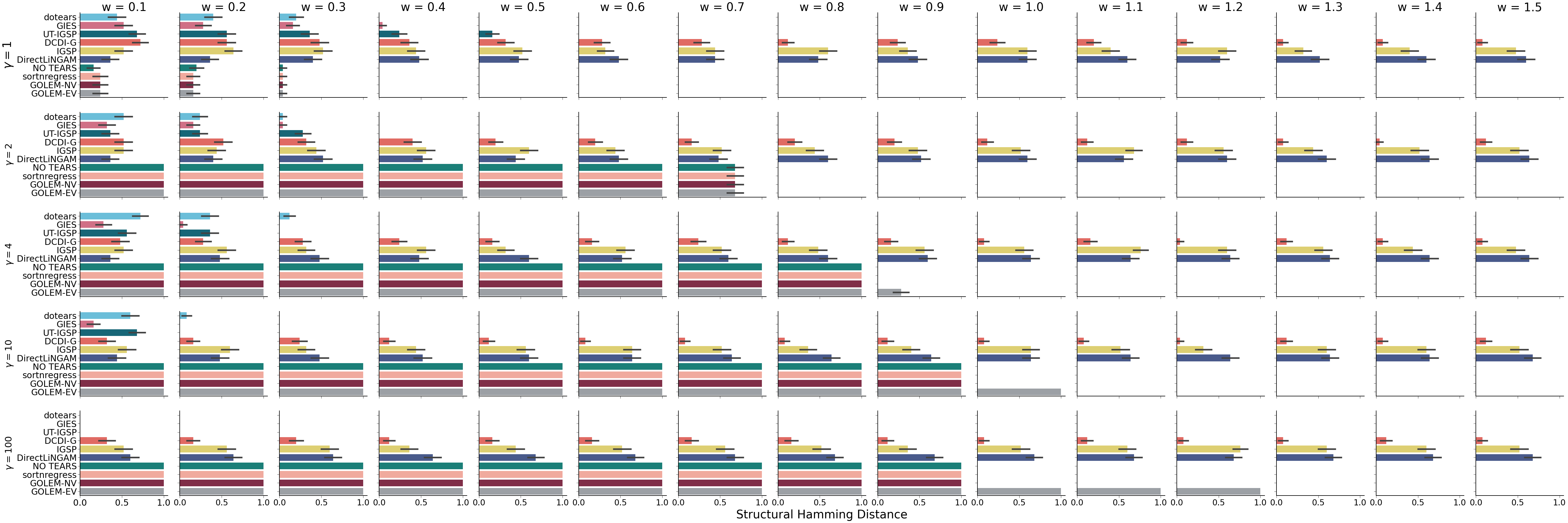
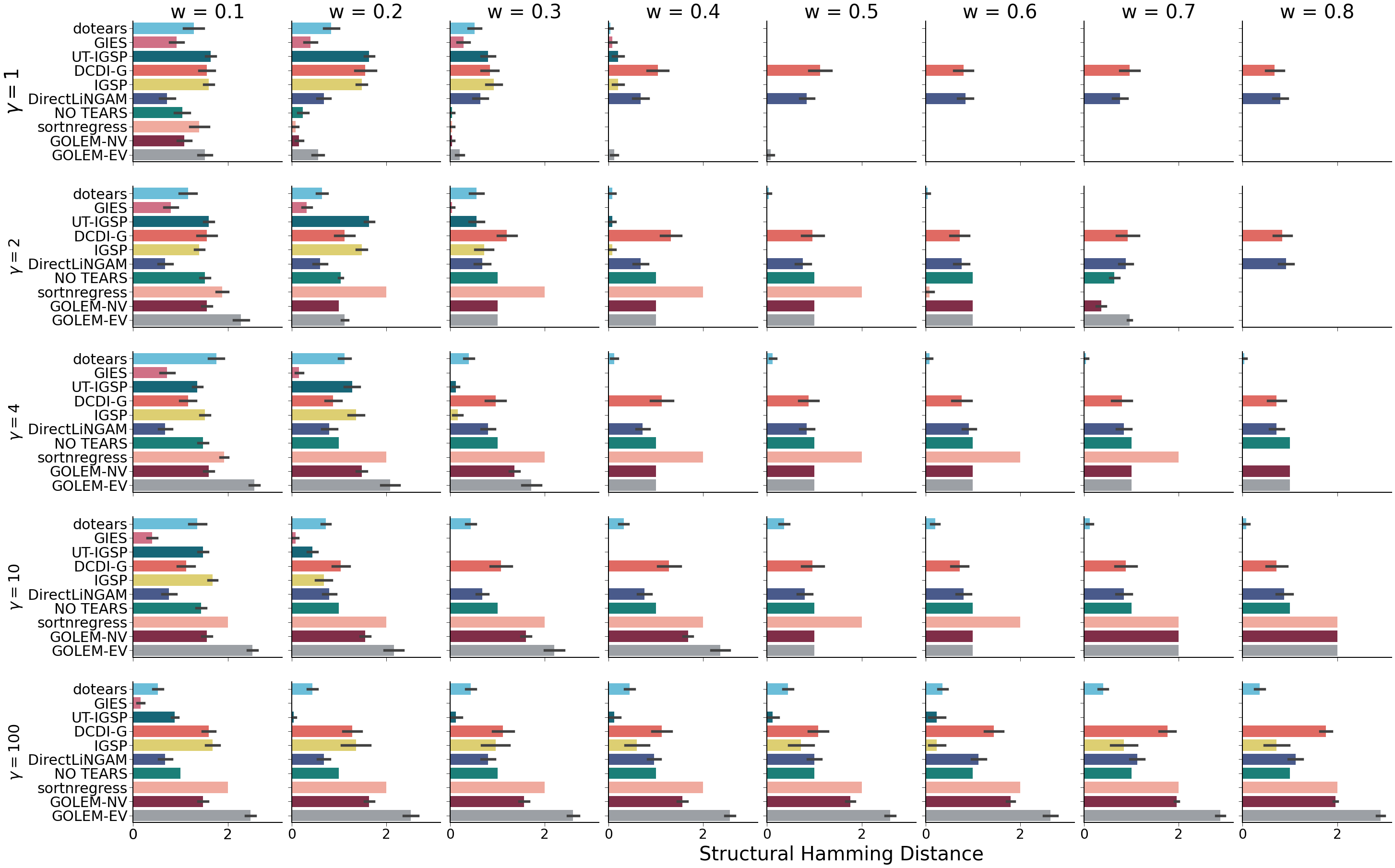
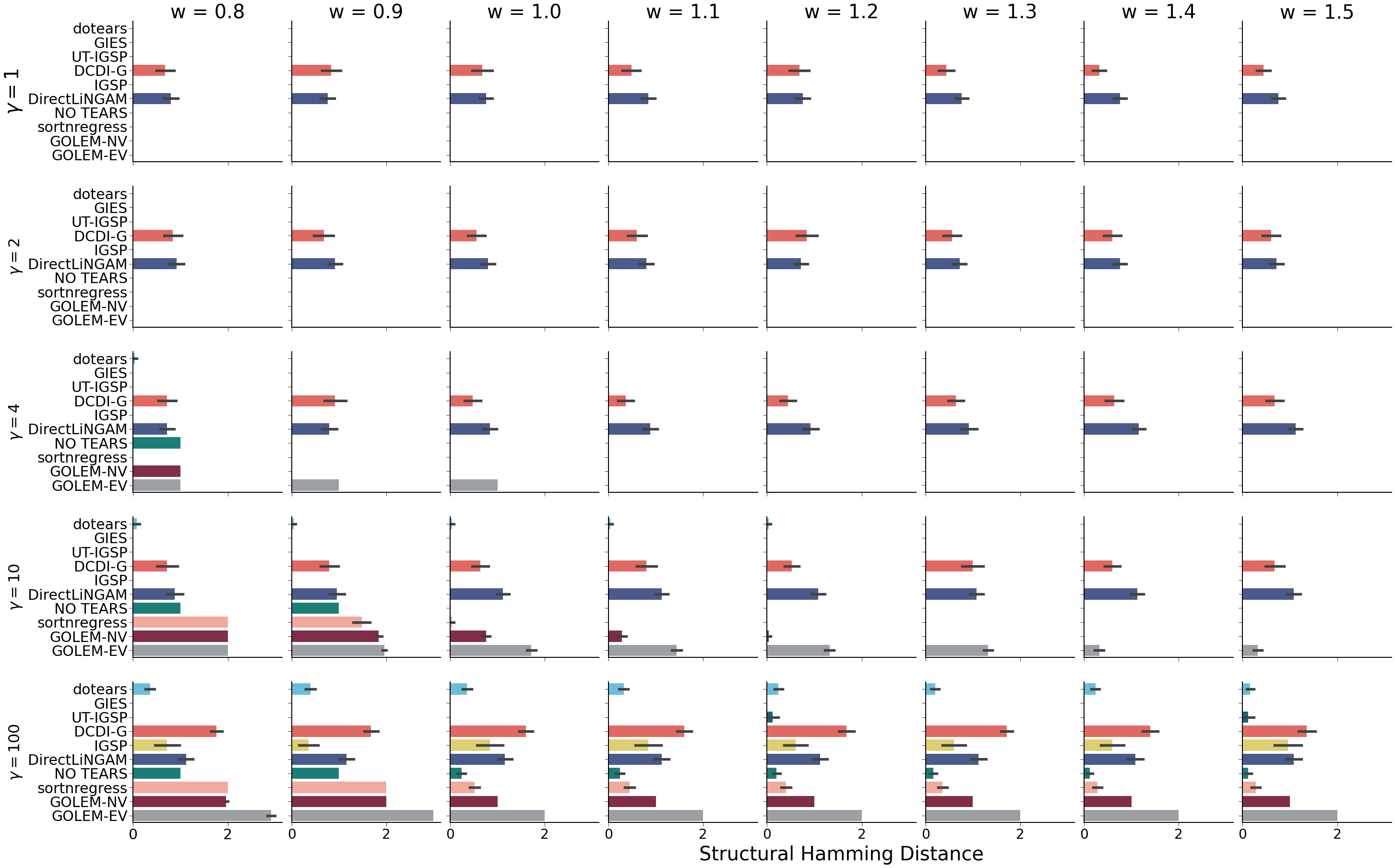
For observational data, we simulate only from the SEM given in Eq. 96, with a sample size $n=3000$. For interventional data, we draw a sample size of $n_{k}=1000$ from each intervention $k$. This gives a total sample size of $n=(p+1)\times 3000$ for interventional data, which matches the sample size of observational data. We set $\alpha=4$. In Section 5.1, we presented empirical results on two node simulations for $(w,\gamma)\in\{0.3,0.5,0.7,0.8,1.0\}\times\{1,2,100\}$. Figure 6 shows the $\ell_{1}$ distance between the ground truth DAG $W_{0}$ and the inferred DAG for each method, for all $(w,\gamma)\in\{0.1,0.2,\dots,1.5\}\times\{1,2,4,10,100\}$. For each parameter combination of $(w,\gamma)$, we draw 25 instances of simulated data for both the interventional and strictly observational case, at the described sample size.

For dotears, sortnregress, and NO TEARS, we set the regularization parameter $\lambda$ to 0, to isolate the performance of the loss function. In GOLEM-EV and GOLEM-NV we set the $\ell_{1}$ regularization parameter $\lambda_{1}$ to 0, but let $\lambda_{2}=5$ to enforce DAG-ness, as recommended by the authors.

Figure 6 , for the full set of simulated $w,\gamma$.

Refer to caption
Figure 6: Full simulations for the two-node DAG for all $(w,\gamma)\in\{0.1,0.2,\dots,1.5\}\times\{1,2,4,10,100\}$, where $X_{1}\overset{w}{\rightarrow}X_{2}$ and $\sigma_{1}^{2}=\gamma\sigma_{2}^{2}$. Methods are compared using SHD (lower is better).

7.5 Full three node simulations

Simulations in the two-node DAG showed that NO TEARS and GOLEM-NV are deterministic functions of the true structure $W$ and the true exogenous variance structure $\Omega_{0}$ (Sections 5.1, 7.4). Simulations in more complex three-node topologies verify determinism of NO TEARS and GOLEM-NV in $W$ and $\Omega_{0}$, but show they are distinct deterministic functions.

We simulate observational and interventional data under the three node chain $X_{1}\overset{w}{\rightarrow}X_{2}\overset{w}{\rightarrow}X_{3}$, the three node collider $X_{1}\overset{w}{\rightarrow}X_{3}\overset{w}{\leftarrow}X_{2}$, and the three node fork $X_{2}\overset{w}{\leftarrow}X_{1}\overset{w}{\rightarrow}X_{3}$. In each topology, we let $\Omega_{0}\coloneqq\begin{pmatrix}\gamma&0&0\\ 0&1&0\\ 0&0&1\end{pmatrix}$, so that $\gamma$ is the exogenous variance of a source node. For simplicity, we constrain the edge weights to be equal, and simulate data under Gaussian exogenous variance for $(w,\gamma)\in\{0.1,\dots,1.5\}\times\{1,2,4,10,100\}$. For interventional data with interventions $i\in\{0,1,2,3\}$, we draw $n_{i}=1000$ observations in all simulations, giving us a total sample size of $n=4000$ that is matched in observational data. As in section 5.1, we set $\alpha=4$, and remove $\ell_{1}$ regularization where appropriate. We benchmark dotears, NO TEARS, sortnregress, GOLEM-EV, GOLEM-NV, DirectLingam, GIES, IGSP, UT-IGSP, and DCDI-G [5, 10, 11, 21, 22, 23, 24, 25, 26].

We evaluate each method by the SHD between the ground truth DAG $W$ and the method inferred DAG. In the two node case, the least squares loss performed identically to the likelihood loss of GOLEM-NV; here, their performances diverge, but remain essentially deterministic functions in $w$ and $\gamma$.

7.5.1 Chain

In the chain, we have the true structure $W_{0}=\begin{pmatrix}0&w&0\\ 0&0&w\\ 0&0&0\end{pmatrix}$. We simulate under the system of SEMs

$\displaystyle X^{(0)}$ $\displaystyle=X^{(0)}W_{0}+\epsilon^{(0)}$ (99)
$\displaystyle X^{(1)}$ $\displaystyle=X^{(1)}W_{0}^{(1)}+\epsilon^{(1)}$
$\displaystyle X^{(2)}$ $\displaystyle=X^{(2)}W_{0}^{(2)}+\epsilon^{(2)},$
$\displaystyle X^{(3)}$ $\displaystyle=X^{(3)}W_{0}^{(3)}+\epsilon^{(3)},$

such that in the observational system

$\displaystyle X_{1}^{(0)}$ $\displaystyle=\epsilon_{1}^{(1)}$ $\displaystyle\epsilon_{1}^{(0)}\sim\mathcal{N}\left(0,\gamma\right)$ (100)
$\displaystyle X_{2}^{(0)}$ $\displaystyle=wX_{1}^{(0)}+\epsilon_{2}^{(0)}$ $\displaystyle\epsilon_{2}^{(0)}\sim\mathcal{N}\left(0,1\right),$
$\displaystyle X_{3}^{(0)}$ $\displaystyle=wX_{2}^{(0)}+\epsilon_{3}^{(0)}$ $\displaystyle\epsilon_{3}^{(0)}\sim\mathcal{N}\left(0,1\right),$

under intervention on node 1 we have

$\displaystyle X_{1}^{(1)}$ $\displaystyle=\epsilon_{1}^{(1)}$ $\displaystyle\epsilon_{1}^{(1)}\sim\mathcal{N}\left(0,\frac{\gamma}{\alpha^{2}}\right)$ (101)
$\displaystyle X_{2}^{(1)}$ $\displaystyle=wX_{1}^{(1)}+\epsilon_{2}^{(1)}$ $\displaystyle\epsilon_{2}^{(1)}\sim\mathcal{N}\left(0,1\right),$
$\displaystyle X_{3}^{(1)}$ $\displaystyle=wX_{2}^{(1)}+\epsilon_{3}^{(1)}$ $\displaystyle\epsilon_{3}^{(1)}\sim\mathcal{N}\left(0,1\right),$

under intervention on node 2

$\displaystyle X_{1}^{(2)}$ $\displaystyle=\epsilon_{1}^{(2)}$ $\displaystyle\epsilon_{1}^{(2)}\sim\mathcal{N}\left(0,\gamma\right)$ (102)
$\displaystyle X_{2}^{(2)}$ $\displaystyle=\epsilon_{2}^{(2)}$ $\displaystyle\epsilon_{2}^{(2)}\sim\mathcal{N}\left(0,\frac{1}{\alpha^{2}}\right),$
$\displaystyle X_{3}^{(2)}$ $\displaystyle=wX_{2}^{(2)}+\epsilon_{3}^{(2)}$ $\displaystyle\epsilon_{3}^{(2)}\sim\mathcal{N}\left(0,1\right),$

and under intervention on node 3

$\displaystyle X_{1}^{(3)}$ $\displaystyle=\epsilon_{1}^{(3)}$ $\displaystyle\epsilon_{1}^{(3)}\sim\mathcal{N}\left(0,\gamma\right)$ (103)
$\displaystyle X_{2}^{(3)}$ $\displaystyle=wX_{1}^{(3)}+\epsilon_{2}^{(3)}$ $\displaystyle\epsilon_{2}^{(3)}\sim\mathcal{N}\left(0,1\right),$
$\displaystyle X_{3}^{(1)}$ $\displaystyle=\epsilon_{3}^{(3)}$ $\displaystyle\epsilon_{3}^{(3)}\sim\mathcal{N}\left(0,\frac{1}{\alpha^{2}}\right).$

Figure 7 shows the full results.

Refer to caption
(a) Results for $w$ in $0.1,\dots,0.8$, inclusive.
Refer to caption
(b) Results for $w$ in $0.8,\dots,1.5$, inclusive.
Figure 7: Full simulations for the chain topology $X_{1}\overset{w}{\rightarrow}X_{2}\overset{w}{\rightarrow}X_{3}$, where $\Omega_{0}=\begin{pmatrix}\gamma&0&0\\ 0&1&0\\ 0&0&1\\ \end{pmatrix}$. We iterate across all $(w,\gamma)\in\{0.1,0.2,\dots,1.5\}\times\{1,2,4,10,100\}$. Methods are compared using SHD (lower is better). (a) shows results for $w$ in $0.1,\dots,0.8$, inclusive, while (b) shows results for $w$ in $0.8,\dots,1.5$, inclusive. $w=0.8$ is repeated across subpanels.

7.5.2 Collider

In the collider, we have the true structure $W_{0}=\begin{pmatrix}0&0&w\\ 0&0&w\\ 0&0&0\end{pmatrix}$. We simulate under the system of SEMs

$\displaystyle X^{(0)}$ $\displaystyle=X^{(0)}W_{0}+\epsilon^{(0)}$ (104)
$\displaystyle X^{(1)}$ $\displaystyle=X^{(1)}W_{0}^{(1)}+\epsilon^{(1)}$
$\displaystyle X^{(2)}$ $\displaystyle=X^{(2)}W_{0}^{(2)}+\epsilon^{(2)},$
$\displaystyle X^{(3)}$ $\displaystyle=X^{(3)}W_{0}^{(3)}+\epsilon^{(3)},$

such that in the observational system

$\displaystyle X_{1}^{(0)}$ $\displaystyle=\epsilon_{1}^{(1)}$ $\displaystyle\epsilon_{1}^{(0)}\sim\mathcal{N}\left(0,\gamma\right)$ (105)
$\displaystyle X_{2}^{(0)}$ $\displaystyle=\epsilon_{2}^{(0)}$ $\displaystyle\epsilon_{2}^{(0)}\sim\mathcal{N}\left(0,1\right),$
$\displaystyle X_{3}^{(0)}$ $\displaystyle=wX_{1}^{(0)}+wX_{2}^{(0)}+\epsilon_{3}^{(0)}$ $\displaystyle\epsilon_{3}^{(0)}\sim\mathcal{N}\left(0,1\right),$

under intervention on node 1 we have

$\displaystyle X_{1}^{(1)}$ $\displaystyle=\epsilon_{1}^{(1)}$ $\displaystyle\epsilon_{1}^{(1)}\sim\mathcal{N}\left(0,\frac{\gamma}{\alpha^{2}}\right)$ (106)
$\displaystyle X_{2}^{(1)}$ $\displaystyle=\epsilon_{2}^{(1)}$ $\displaystyle\epsilon_{2}^{(1)}\sim\mathcal{N}\left(0,1\right),$
$\displaystyle X_{3}^{(1)}$ $\displaystyle=wX_{1}^{(1)}+wX_{2}^{(1)}+\epsilon_{3}^{(1)}$ $\displaystyle\epsilon_{3}^{(1)}\sim\mathcal{N}\left(0,1\right),$

under intervention on node 2

$\displaystyle X_{1}^{(2)}$ $\displaystyle=\epsilon_{1}^{(2)}$ $\displaystyle\epsilon_{1}^{(2)}\sim\mathcal{N}\left(0,\gamma\right)$ (107)
$\displaystyle X_{2}^{(2)}$ $\displaystyle=\epsilon_{2}^{(2)}$ $\displaystyle\epsilon_{2}^{(2)}\sim\mathcal{N}\left(0,\frac{1}{\alpha^{2}}\right),$
$\displaystyle X_{3}^{(2)}$ $\displaystyle=wX_{1}^{(2)}+wX_{2}^{(2)}+\epsilon_{3}^{(2)}$ $\displaystyle\epsilon_{3}^{(2)}\sim\mathcal{N}\left(0,1\right),$

and under intervention on node 3

$\displaystyle X_{1}^{(3)}$ $\displaystyle=\epsilon_{1}^{(3)}$ $\displaystyle\epsilon_{1}^{(3)}\sim\mathcal{N}\left(0,\gamma\right)$ (108)
$\displaystyle X_{2}^{(3)}$ $\displaystyle=\epsilon_{2}^{(3)}$ $\displaystyle\epsilon_{2}^{(3)}\sim\mathcal{N}\left(0,1\right),$
$\displaystyle X_{3}^{(1)}$ $\displaystyle=\epsilon_{3}^{(3)}$ $\displaystyle\epsilon_{3}^{(3)}\sim\mathcal{N}\left(0,\frac{1}{\alpha^{2}}\right).$
Refer to caption
(a) Results for $w$ in $0.1,\dots,0.8$, inclusive.
Refer to caption
(b) Results for $w$ in $0.8,\dots,1.5$, inclusive.
Figure 8: Full simulations for the collider topology $X_{1}\overset{w}{\rightarrow}X_{3}\overset{w}{\leftarrow}X_{2}$, where $\Omega_{0}=\begin{pmatrix}\gamma&0&0\\ 0&1&0\\ 0&0&1\\ \end{pmatrix}$. We iterate across all $(w,\gamma)\in\{0.1,0.2,\dots,1.5\}\times\{1,2,4,10,100\}$. Methods are compared using SHD (lower is better). (a) shows results for $w$ in $0.1,\dots,0.8$, inclusive, while (b) shows results for $w$ in $0.8,\dots,1.5$, inclusive. $w=0.8$ is repeated across subpanels.

7.5.3 Fork

In the collider, we have the true structure $W_{0}=\begin{pmatrix}0&w&w\\ 0&0&0\\ 0&0&0\end{pmatrix}$. We simulate under the system of SEMs

$\displaystyle X^{(0)}$ $\displaystyle=X^{(0)}W_{0}+\epsilon^{(0)}$ (109)
$\displaystyle X^{(1)}$ $\displaystyle=X^{(1)}W_{0}^{(1)}+\epsilon^{(1)}$
$\displaystyle X^{(2)}$ $\displaystyle=X^{(2)}W_{0}^{(2)}+\epsilon^{(2)},$
$\displaystyle X^{(3)}$ $\displaystyle=X^{(3)}W_{0}^{(3)}+\epsilon^{(3)},$

such that in the observational system

$\displaystyle X_{1}^{(0)}$ $\displaystyle=\epsilon_{1}^{(1)}$ $\displaystyle\epsilon_{1}^{(0)}\sim\mathcal{N}\left(0,\gamma\right)$ (110)
$\displaystyle X_{2}^{(0)}$ $\displaystyle=wX_{1}^{(0)}+\epsilon_{2}^{(0)}$ $\displaystyle\epsilon_{2}^{(0)}\sim\mathcal{N}\left(0,1\right),$
$\displaystyle X_{3}^{(0)}$ $\displaystyle=wX_{1}^{(0)}+\epsilon_{3}^{(0)}$ $\displaystyle\epsilon_{3}^{(0)}\sim\mathcal{N}\left(0,1\right),$

under intervention on node 1 we have

$\displaystyle X_{1}^{(1)}$ $\displaystyle=\epsilon_{1}^{(1)}$ $\displaystyle\epsilon_{1}^{(1)}\sim\mathcal{N}\left(0,\frac{\gamma}{\alpha^{2}}\right)$ (111)
$\displaystyle X_{2}^{(1)}$ $\displaystyle=wX_{1}^{(0)}+\epsilon_{2}^{(1)}$ $\displaystyle\epsilon_{2}^{(1)}\sim\mathcal{N}\left(0,1\right),$
$\displaystyle X_{3}^{(1)}$ $\displaystyle=wX_{1}^{(1)}+\epsilon_{3}^{(1)}$ $\displaystyle\epsilon_{3}^{(1)}\sim\mathcal{N}\left(0,1\right),$

under intervention on node 2

$\displaystyle X_{1}^{(2)}$ $\displaystyle=\epsilon_{1}^{(2)}$ $\displaystyle\epsilon_{1}^{(2)}\sim\mathcal{N}\left(0,\gamma\right)$ (112)
$\displaystyle X_{2}^{(2)}$ $\displaystyle=\epsilon_{2}^{(2)}$ $\displaystyle\epsilon_{2}^{(2)}\sim\mathcal{N}\left(0,\frac{1}{\alpha^{2}}\right),$
$\displaystyle X_{3}^{(2)}$ $\displaystyle=wX_{1}^{(2)}+\epsilon_{3}^{(2)}$ $\displaystyle\epsilon_{3}^{(2)}\sim\mathcal{N}\left(0,1\right),$

and under intervention on node 3

$\displaystyle X_{1}^{(3)}$ $\displaystyle=\epsilon_{1}^{(3)}$ $\displaystyle\epsilon_{1}^{(3)}\sim\mathcal{N}\left(0,\gamma\right)$ (113)
$\displaystyle X_{2}^{(3)}$ $\displaystyle=wX_{1}^{(3)}+\epsilon_{2}^{(3)}$ $\displaystyle\epsilon_{2}^{(3)}\sim\mathcal{N}\left(0,1\right),$
$\displaystyle X_{3}^{(1)}$ $\displaystyle=\epsilon_{3}^{(3)}$ $\displaystyle\epsilon_{3}^{(3)}\sim\mathcal{N}\left(0,\frac{1}{\alpha^{2}}\right).$
Refer to caption
(a) Results for $w$ in $0.1,\dots,0.8$, inclusive.
Refer to caption
(b) Results for $w$ in $0.8,\dots,1.5$, inclusive.
Figure 9: Full simulations for the fork topology $X_{2}\overset{w}{\leftarrow}X_{1}\overset{w}{\rightarrow}X_{3}$, where $\Omega_{0}=\begin{pmatrix}\gamma&0&0\\ 0&1&0\\ 0&0&1\\ \end{pmatrix}$. We iterate across all $(w,\gamma)\in\{0.1,0.2,\dots,1.5\}\times\{1,2,4,10,100\}$. Methods are compared using SHD (lower is better). (a) shows results for $w$ in $0.1,\dots,0.8$, inclusive, while (b) shows results for $w$ in $0.8,\dots,1.5$, inclusive. $w=0.8$ is repeated across subpanels.

7.6 Large random graph simulations

7.6.1 Data generation

For evaluation, data is generated for DAGs with $p=50$ nodes. Structures are drawn from both Erdős-Rényi (ER) and Scale-Free (SF) DAGs [27, 28]. We parameterize ER graphs as ER-$r$ and SF graphs as SF-$z$, where $r\in[0,1]$ represents the probability of assignment of each individual edge, whereas $z\in\mathbb{Z}$ is the integer number of edges assigned per node.

We simulate under two parameterizations $\{\text{Low Density, High Density}\}$ of the edge densities $(r,z)$. In the “Low Density" parameterization, we match the number of expected edges for simulations found in Reisach et al., i.e. $(r,z)=(0.08,2)$. To evaluate performance on higher density topologies, we also give “High Density" parameterizations, where $(r,z)=(0.2,4)$.

Given an edge density scenario, we simulate under two parameterizations of the edge weights. In the “Strong Effects" parameterization, $w\sim\text{Unif}\left([-2.0,0.5]\cup[0.5,2.0]\right)$. In this scenario, for an edge $w_{ij}$ the nodes $i$ and $j$ are varsortable with probability at least $\frac{2}{3}$, when $|w|\geq 1$ [11]. We therefore also give the “Weak Effects" parameterization, which edge weights are drawn from $w\sim\text{Unif}\left([-1.0,0.3]\cup[0.3,1.0]\right)$ such that $|w|\leq 1$ is guaranteed. Here, there is no guarantee any two nodes will be varsortable (although they may be in practice, as a function of $\Omega_{0}$) [11, 12]. Table 1 summarizes all four possible simulation parameterizations.

For each node $i$, we draw $\sigma_{i}\sim\text{Unif}\left([0.5,2.0]\right)$, and draw $n_{0}$ observations from $\boldsymbol{\epsilon}_{i}^{(0)}\sim\mathcal{N}\left(0,\sigma_{i}^{2}\right)$. For each DAG we generate an instance of observational data, where $n_{0}=(p+1)*n_{k}=5100$, and an instance of interventional data, where $n_{k}=100$ for all $k=0\dots p$ to match sample size. We set the distribution of $\epsilon_{i}^{(k)}$ according to Assumptions 2 and 3 for $\alpha=4$.

Simulation Type Topology $w$
Low Density , Strong Effects ER-0.08 OR SF-2 $\text{Unif}\left([-2.0,-0.5]\cup[0.5,2.0]\right)$
Low Density , Weak Effects ER-0.08 OR SF-2 $\text{Unif}\left([-1.0,-0.3]\cup[0.3,1.0]\right)$
High Density , Strong Effects ER-0.2 OR SF-4 $\text{Unif}\left([-2.0,-0.5]\cup[0.5,2.0]\right)$
High Density , Weak Effects ER-0.2 OR SF-4 $\text{Unif}\left([-1.0,-0.3]\cup[0.3,1.0]\right)$
Table 1: For each simulation type, we provide the parameterizations of the Erdős-Rényi and Scale-Free topologies, the distribution on the drawn edge weights, and the distribution on the standard deviations of the exogenous variance.

For dotears, NO TEARS, sortnregress, GOLEM-EV, and GOLEM-NV, 5-fold cross-validation was performed to select the regularization parameters. For each drawn DAG, a separate data instance of interventional and observational data was re-drawn from the same distribution specifically for cross-validation. After choosing a $\lambda$ (or for GOLEM-EV and GOLEM-NV, the set $(\lambda_{1},\lambda_{2})$) from the data for cross-validation, the methods were evaluated on the original simulated data. For dotears, NO TEARS, and sortnregress, 5-fold cross-validation was performed across the grid $\lambda\in\{.001,.01,.1,1,10,100\}$. For GOLEM-EV and GOLEM-NV, 5-fold cross-validation was performed across the grid $\lambda_{1}\times\lambda_{2}\in\{.001,.01,.1,1,10,100\}\times\{.05,.5,5,50\}$.

7.6.2 Benchmarking

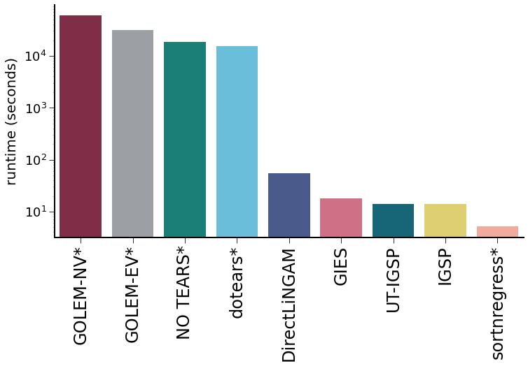
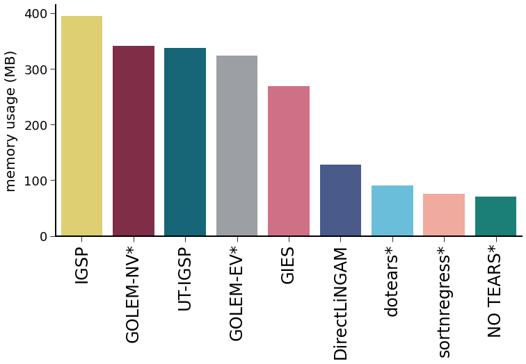
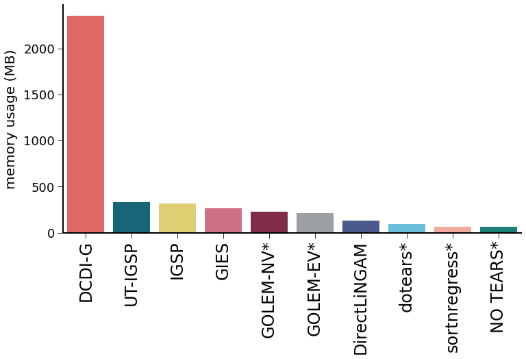
In Figure 10, we benchmark wallclock time and memory usage for all methods in $p=50$ simulations [30]. All continuous optimization methods (dotears, NO TEARS, GOLEM-EV, and GOLEM-NV) have significantly higher average runtimes than other methods, which is partially explained by cross-validation procedures. dotears has relatively light memory usage, outperformed only by NO TEARS and sortnregress.

Refer to caption
(a) Wallclock time across all $p=50$ simulations in seconds. Y-axis is in log-scale.
Refer to caption
(b) Memory usage across all $p=50$ simulations, defined as the maximum unique set size used by the process, or max_uss (see psutil documentation).
Figure 10: Comparison of mean runtime (a) and mean memory usage (b) between methods across all $p=50$ simulations. For both figures, standard errors were uninformative and thus removed.

7.6.3 Thresholding on large simulation results

Edge thresholding for weighted adjacency matrices is necessary for accurate evaluation using SHD, but the choice of threshold can feel arbitrary. We find that methods are generally robust to thresholding choice, following similar results from [11].

Figure 11 examines the effect on thresholding of small weights in $W$ in large random DAG simulations, for methods that infer weighted adjacency matrices (dotears, NO TEARS, sortnregress, DirectLiNGAM, GOLEM-NV, and GOLEM-EV) [10, 11, 21, 26]. For simplicity, we summarize simulations in terms of the generative edge distribution. Simulations with “Weak Effects", $w\sim\text{Unif}\left([-1.0,-0.3]\cup[0.3,1.0]\right)$, are shown in Figure 11(a); simulations with “Strong Effects", $w\sim\text{Unif}\left([-2.0,-0.5]\cup[0.5,2.0]\right)$ are shown in Figure 11(b). We compare the SHD between the ground truth adjacency matrix and the inferred adjacency matrix for each method at all thresholds between 0 and the absolute lower bound of the true edge weight distribution (0.3 for “Weak Effects", 0.5 for “Strong Effects"). Any edge whose magnitude is below the chosen threshold is set to 0 for SHD evaluation.

Refer to caption
(a) Structural Hamming Distance (lower is better) as a function of $\hat{w}$ threshold for “Weak Effects" scenarios, where $w\sim\text{Unif}\left([-1.0,-0.3]\cup[0.3,1.0]\right)$.
Refer to caption
(b) Structural Hamming Distance (lower is better) as a function of $\hat{w}$ threshold for “Strong Effects" scenarios, where $w\sim\text{Unif}\left([-2.0,-0.5]\cup[0.5,2.0]\right)$.
Figure 11: Structural Hamming Distance (lower is better) as a function of thresholding choice for $p=50$ simulations detailed in 7.6.1. Parameterizations with “Weak Effects", $w\sim\text{Unif}\left([-1.0,-0.3]\cup[0.3,1.0]\right)$, are consolidated in (a), while parameterizations with “Strong Effects", $w\sim\text{Unif}\left([-2.0,-0.5]\cup[0.5,2.0]\right)$, are consolidated in (b). Standard errors were uninformative and thus removed.

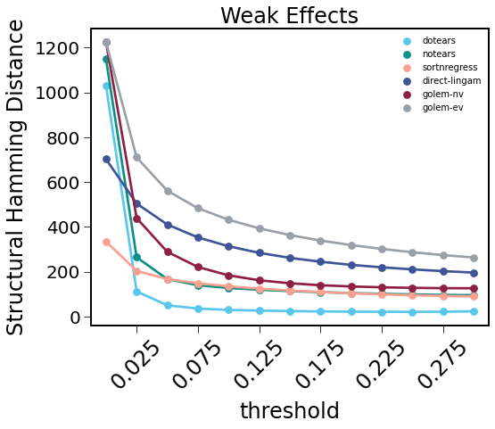
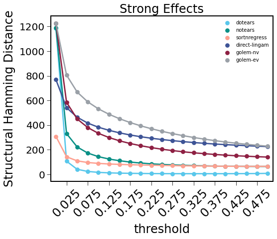
Figure 11 shows that thresholding is necessary for evaluation of SHD between weighted adjacency matrices, but also that methods are generally robust to thresholding choice. Without thresholding (equivalently, a threshold of 0), SHD results are inflated, but recover even at low thresholds.

7.6.4 Edge weight estimation for large random simulations

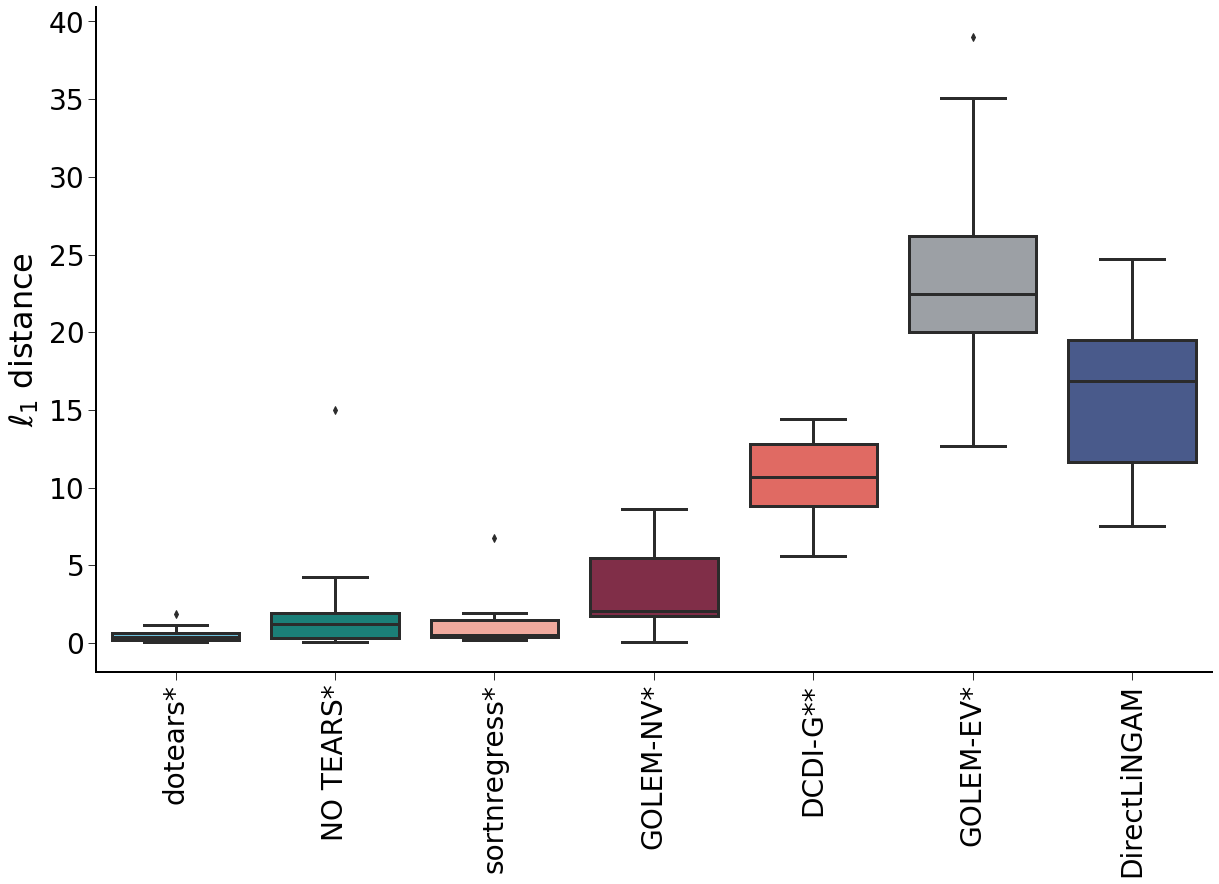
Accurate estimation of edge weights is important for understanding structure. Figure 5 gives results on structural recovery through SHD, but does not inform edge weight recovery. To measure edge weight recovery we use $\ell_{1}$ distance, defined as the vector $\ell_{1}$ norm between the flattened true weighted adjacency matrix and the flattened inferred weighted adjacency matrix. $\ell_{1}$ distance gives information on both structure recovery and edge weight estimation simultaneously. In Figure 12, we benchmark the recovery of edge weights for methods that return a weighted adjacency matrix (dotears, sortnregress, NO TEARS, GOLEM-EV, GOLEM-NV, DirectLiNGAM [10, 11, 21, 26]) for simulations given in 7.6.1. For fairness, we exclude methods that only return a binary adjacency matrix. Methods are thresholded in the same manner as in Figure 5.

Refer to caption
Figure 12: Methodological comparison of structure learning methods on large random graphs ($p$ = 50) using $\ell_{1}$ distance (lower is better). Each row represents simulations drawn with a topology in {Erdős-Rényi, Scale Free}, respectively, and each column represents a different parameterization of edge density and edge weights ordered in terms of increasing difficulty. For details, see Table 1. 100 simulations were drawn for each set of parameters with sample size $(p+1)*100=5100$, and * indicates methods performed with 5-fold cross-validation on a separate draw from the same distribution. Y-axis scales are not shared between figures. Methods are sorted, left to right, by strongest average performance across all simulations. GIES, IGSP, and UT-IGSP infer binary edges and are therefore omitted for fairness.

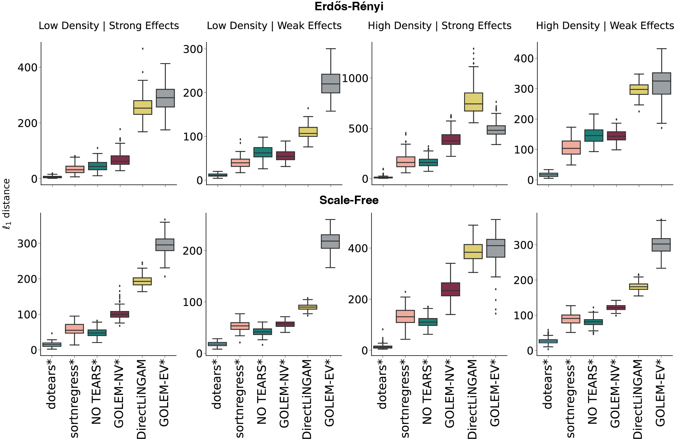
dotears outperforms all other methods in terms of effect size recovery. In addition, the relative ordering of the methods stays consistent with Figure 5.

7.6.5 Statistical significance of SHD distribution difference

For each method, and across all simulations in Section 7.6.1, we compare the SHD distributions, marginalized across all simulation parameterizations, against that of dotears. For each method, we perform a one-sided Mann-Whitney U test to test difference between the method’s SHD distribution and the SHD distribution of dotears. The resulting p-values are reported in Table 2, and are significant for all methods.

Method p-value
GIES 2.85e-75
sortnregress 4.30e-220
NO TEARS 5.38e-231
GOLEM-NV 3.92e-258
DirectLiNGAM 3.88e-263
GOLEM-EV 3.88e-263
IGSP 4.10e-263
UT-IGSP 4.51e-263
Table 2: p-value from asymptotic one-sided Mann-Whitney U test comparing distribution of indicated method SHD against distribution of dotears SHD.

7.6.6 Incorporation of interventional loss

We note that inferring $W$ from strictly observational data, given $\hat{\Omega}_{0}$ from interventional data, has convenient theoretical properties but ignores the majority of our data. Figure 13 compares the performance, in Structural Hamming Distance, of dotears using both observational and interventional data $\left(\mathcal{L}_{\hat{\Omega}_{0}}\left(W^{(k)},\boldsymbol{X}^{(k)}\right)\text{ for }k=0\dots p\right)$ with dotears using only observational data $\left(\mathcal{L}_{\hat{\Omega}_{0}}\left(W^{(k)},\boldsymbol{X}^{(k)}\right)\text{ for }k=0\right)$. We use the simulations drawn in Section 7.6.1, aggregated across all scenarios in Table 1. Note that $\hat{\Omega}_{0}$ is estimated identically for both.

Refer to caption
Figure 13: Comparison of dotears performance when using only $\mathcal{L}_{\hat{\Omega}_{0}}\left(W^{(k)},\boldsymbol{X}^{(k)}\right)$ for observational data ($k=0$), right, and when including interventional data ($k=0\dots p$), left. Methods are run on simulation data generated in Section 7.6.1, aggregated across all scenarios in Table 1. Methods are compared using Structural Hamming Distance (lower is better).

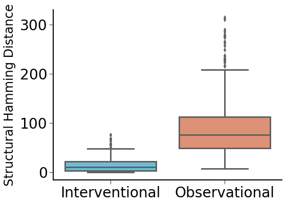
As expected, restricting dotears to inference only using the observational data (Figure 13, right) drastically decreases performance when compared to inference using both observational and interventional data (Figure 13, left). This motivates including $k=1\dots p$ into the loss and proving consistency for all $k$.

7.7 DCDI-G

The memory usage of DCDI-G was prohibitive for the large simulations ($p=50$) in 7.6.1, and cross-validation was not easily supported. We evaluate DCDI-G on smaller simulations based on Section 7.6.1, on random DAGs such that $p=10$ [25]. As before, we evaluate methods on both structural recovery and edge weight estimation using SHD and $\ell_{1}$ distance, respectively. DCDI-G returns a binary adjacency matrix, and is excluded from evaluation on edge weight recovery.

7.7.1 Data generation

Random DAGs are parameterized as in 7.6.1; for $p=10$ simulations, we choose $(r,z)=(0.2,4)$, or equivalently “High Density" simulations. Similarly, we draw edges from $w\sim\text{Unif}\left([-2.0,0.5]\cup[0.5,2.0]\right)$, as in the “Strong Effects" scenario. For each node $i$, we draw $\sigma_{i}\sim\text{Unif}\left([0.5,2.0]\right)$. Sample sizes are matched between observational and interventional data. For interventional data, we draw $n_{k}=100$ observations per intervention $k=0\dots p$, for a total of $1100$ observations across interventions. For observational data, we draw $n_{0}=1100$ observations to match sample size. $\alpha=4$ is set in all draws, and $10$ total simulations were drawn for each random DAG type (ER or SF).

For each value of $\lambda\in\{.001,.01,.1,1,10,100\}$, we ran DCDI-G using the chosen $\lambda$ value on the drawn data. The best-performing output in terms of SHD was selected for comparison against the other methods. Note that cross-validation procedure is favorable to DCDI-G compared to other methods.

7.7.2 Results

Figure 14 shows method results in SHD, while Figure 15 shows method results in $\ell_{1}$ distance. In all figures DCDI-G is denoted with **, to indicate its favorable cross-validation procedure.

Refer to caption
(a) Performance in SHD (lower is better) on $p=10$ Erdős-Rényi-0.2 graphs.
Refer to caption
(b) Performance in SHD (lower is better) on $p=10$ Scale Free-4 graphs.
Figure 14: Comparison of performance of structure learning methods on random graphs for $p=10$ using Structural Hamming Distance. Simulations were drawn from Erdős-Rényi-0.2 and Scale Free-4 graphs, for edge weights $w\in\text{Unif}\left([-2.0,0.5]\cup[0.5,2.0]\right)$. 10 simulations were drawn for each set of parameters with sample size $(p+1)\times 100=1100$. * indicates methods performed with 5-fold cross-validation on a separate draw from the same distribution. DCDI-G is denoted with **, to indicate its more favorable cross-validation procedure. In each simulation, DCDI-G was run for all values of $\lambda$ and the best-performing result was selected. Methods are sorted, left to right, by average performance across all parameterizations.
Refer to caption
(a) Performance of structure learning methods in $\ell_{1}$ distance on $p=10$ ER-0.2 graphs (lower is better).
Refer to caption
(b) Performance of structure learning methods in $\ell_{1}$ distance on $p=10$ SF-4 graphs (lower is better).
Figure 15: Comparison of performance of structure learning methods on random graphs for $p=10$ using $\ell_{1}$ distance. Simulations were drawn from Erdős-Rényi-0.2 and Scale Free-4 graphs, for edge weights $w\in\text{Unif}\left([-2.0,0.5]\cup[0.5,2.0]\right)$. 10 simulations were drawn for each set of parameters with sample size $(p+1)*100=1100$. Methods are sorted, left to right, by average performance across all parameterizations.

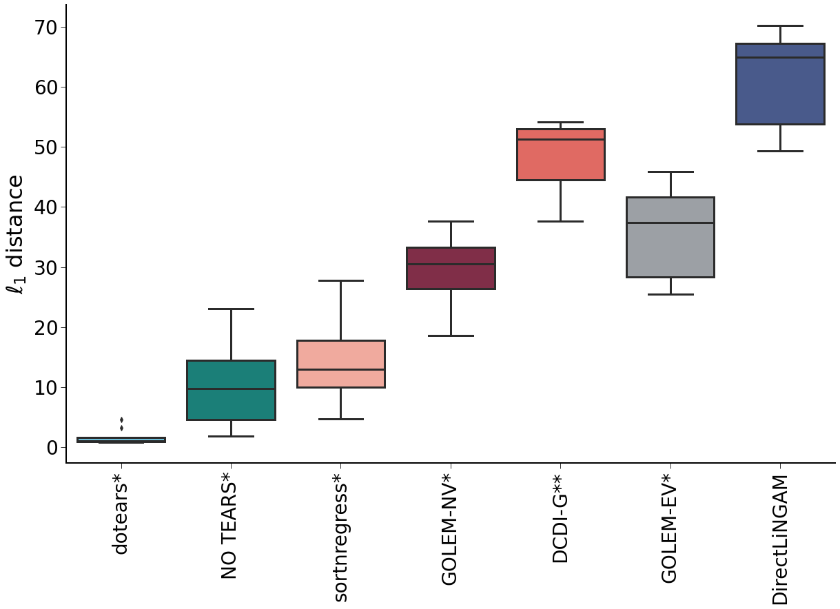
DCDI-G performs poorly in Erdős-Rényi-0.2 graphs, and slightly worse than sortnregress in Scale Free-4 graphs. We note that Erdős-Rényi-0.2 graphs have $9$ edges in expectation, while Scale Free-4 graphs have $30$ edges (see igraph implementation for details [31]), out of a possible 45 total edges. The increased density of Scale Free-4 graphs may account for this discrepancy.

dotears is still the best performing method in small graphs in both structural recovery and edge weight recovery. GIES improves from the 4th best performing method in $p=50$ simulations (Figure 5) to the second-best performing method in $p=10$ simulations. We hypothesize that this relative performance increase is due to the greedy nature of GIES, which is more suited to inference on smaller graphs. Outside of GIES and the addition of DCDI-G, the relative ordering of method performance does not change from Figure 5.

7.7.3 Benchmarking

For small random graph simulations, we evaluate the wallclock time and memory usage for all methods, including DCDI-G, in Figure 16. We evaluate only a single run of DCDI-G, for a single value of $\lambda$, and not the entire cross-validation procedure. As such, DCDI-G is not denoted with the double asterisks ** in Figure 14; cross-validation of DCDI-G will necessitate more resources than shown. Even without considering cross-validation, DCDI-G is a clear outlier in terms of memory usage (Figure 16(b)).

Refer to caption
(a) Wallclock time in $p=10$ simulations in seconds. Y-axis is in log-scale.
Refer to caption
(b) Memory usage in $p=10$ simulations, defined as the maximum unique set size used by the process, or max_uss (see psutil documentation).
Figure 16: Comparison of mean runtime (a) and mean memory usage (b) between methods in $p=10$ simulations. For both figures, standard errors were uninformative and thus removed. DCDI-G is denoted without the double asterisks in Figure 14 because the results represent a single run of DCDI-G for a single value of $\lambda$, and not the total runtime or memory usage for a cross-validated run of DCDI-G.

Code Availability

Code to reproduce the experiments in this paper, as well as a working implementation of dotears, is available at https://github.com/asxue/dotears/.

Acknowledgments

AX was supported by the NIH Training Grant in Genomic Analysis and Interpretation T32HG002536. This work was partially funded by HHMI Hanna H Gray and Sloan fellows programs to HP. This work was partially funded by NIH grant (R35GM125055) and NSF grants (CAREER-1943497, IIS-2106908) to SS. We thank Nathan LaPierre for helpful conversations.