Fast global convergence of gradient descent for low-rank matrix approximation

Abstract

This paper investigates gradient descent for solving low-rank matrix approximation problems. We begin by establishing the local linear convergence of gradient descent for symmetric matrix approximation. Building on this result, we prove the rapid global convergence of gradient descent, particularly when initialized with small random values. Remarkably, we show that even with moderate random initialization, which includes small random initialization as a special case, gradient descent achieves fast global convergence in scenarios where the top eigenvalues are identical. Furthermore, we extend our analysis to address asymmetric matrix approximation problems and investigate the effectiveness of a retraction-free eigenspace computation method. Numerical experiments strongly support our theory. In particular, the retraction-free algorithm outperforms the corresponding Riemannian gradient descent method, resulting in a significant 29% reduction in runtime.

1 Introduction

Low-rank problems play a crucial role in statistics and engineering. One fundamental problem in low-rank approximation aims to find a low-rank matrix $\bm{\Sigma}_{r}$ that provides the best approximation to a given positive semi-definite matrix $\bm{\Sigma}\in\mathbb{R}^{d\times d}$, subject to the constraint:

$$\bm{\Sigma}_{r}=\mathop{\mathrm{argmin}}_{\bm{M}}\|\bm{\Sigma}-\bm{M}\|_{{\scriptstyle\mathrm{F}}}^{2},\quad\textnormal{s.t. }{\rm rank}(\bm{M})\leq r.$$ (1.1)

This problem is commonly referred to as symmetric low-rank matrix approximation, and it is well-known that $\bm{\Sigma}_{r}=\sum_{i=1}^{r}\lambda_{i}^{*}\bm{e}_{i}\bm{e}_{i}^{\top}$, where $\lambda_{i}^{*},\bm{e}_{i}$ denote the $i$-th leading eigenvalue and eigenvector of $\bm{\Sigma}$. Thus $\bm{\Sigma}_{r}$ can be obtained by naively performing eigen-decomposition.

In this paper, we employ the Burer-Montario factorization $\bm{M}=\bm{X}\bm{X}^{\top}$ with the low-rank factor $\bm{X}\in\mathbb{R}^{d\times r}$ (Burer and Monteiro, 2003, 2005) to recover $\bm{\Sigma}_{r}=\bm{X}^{*}\bm{X}^{*\top}$ by solving the following non-convex optimization problem:

$$\bm{X}^{*}=\mathop{\mathrm{argmin}}_{\bm{X}\in\mathbb{R}^{d\times r}}\|\bm{\Sigma}-\bm{X}\bm{X}^{\top}\|_{{\scriptstyle\mathrm{F}}}^{2}.$$ (1.2)

Despite the non-convex nature of this problem, it is often computationally efficient to solve (1.2) using gradient descent, which follows the update rule:

$$\bm{X}_{t+1}=\bm{X}_{t}+\eta(\bm{\Sigma}-\bm{X}_{t}\bm{X}_{t}^{\top})\bm{X}_{t},\quad t=0,1,\ldots,$$ (1.3)

where $\bm{X}_{0}\in\mathbb{R}^{d\times r}$ represents the initialization point, and $\eta$ is the learning rate. By adopting this economical representation of the low-rank matrix, our approach offers several computational advantages, including reduced storage requirements, affordable per-iteration computational cost, parallelizability, and scalability to handle large-scale problems.

The optimization properties of the first-order algorithm (1.3) for the non-convex problem (1.2) are still not fully understood. Zhu et al. (2018, 2021) showed that problem (1.2) does not contain spurious local minima, and all saddle points are strict. Lee et al. (2019) further proved that gradient descent almost surely converges to the global minima, but did not provide any convergence rate results. In fact, Du et al. (2017) demonstrated that there exist problems such that GD can take exponential time to escape the saddle points when initialized randomly. Towards characterizing the convergence rate, recent research has focused on the implicit regularization of gradient descent with small random initialization (Jiang et al., 2022; Stöger and Soltanolkotabi, 2021). These studies revealed that gradient descent, with a small random initialization, quickly approaches an $\epsilon$-neighborhood of the global minima, where $\epsilon$ is a small constant depending on the initialization. These results provide that gradient descent can achieve reasonable approximate solutions but are still one step away from global convergence rate results, due to the lack of local convergence properties. Recently, in the case when $\bm{\Sigma}$ is of exact rank $r$, Zhu et al. (2021) showed that problem (1.2) satisfies a certain local regularity condition, leading to the linear convergence of gradient descent with a good enough local initialization. However, extending their analysis to the general $\bm{\Sigma}$ case remains challenging and unknown.

The goal of this paper is to establish the local linear convergence of gradient descent (1.3). To accomplish this, we introduce a novel dynamic analysis technique. We begin by defining a local region surrounding the global minima of problem (1.2) and prove that it acts as an absorbing region for gradient descent, preventing the solution sequence from leaving once it enters. Next, we show that within this region, the noise-to-signal ratio of the sequence, to be defined later, converges linearly to zero. This property allows us to establish the local linear convergence.

As a result of the local linear convergence, we obtain fast global convergence for gradient descent (1.3) with small random initialization. Furthermore, we consider a special case where the leading eigenvalues of $\bm{\Sigma}$ are identical. In this scenario, we prove that even with moderate random initialization, gradient descent still achieves fast convergence to the global minima. This is the first result that relaxes the requirement of small initialization for $r\geq 1$. In general, we conjecture that gradient descent with moderate random initialization, which includes small random initialization as a special case, also achieves fast global convergence.

Finally, we extend our analysis to cover asymmetric matrix approximation problems. We also provide an application to eigenspace computation. Specifically, we show that the following retraction-free Riemannian gradient descent algorithm can efficiently compute the leading eigenspace of a given positive semi-definite matrix $\bm{\Sigma}\in\mathbb{R}^{d\times d}$:

$$\bm{L}_{t+1}=\bm{L}_{t}+\eta(\bm{I}_{d}-\bm{L}_{t}\bm{L}_{t}^{\top})\bm{\Sigma}\bm{L}_{t},$$ (1.4)

where $\bm{L}_{0}\in\mathbb{R}^{d\times r}$ represents the initialization point, and $\eta$ is the learning rate. We show that $\bm{L}_{t}\bm{L}_{t}^{\top}$ rapidly converges to the projection matrix associated with the top $r$ eigenspace of $\bm{\Sigma}$. Our theory builds on the connection between (1.4) and a symmetric matrix approximation problem. Through numerical experiments, we demonstrate that the retraction-free method outperforms the original Riemannian gradient descent method, resulting in a 29% reduction in runtime.

Notation

We adopt the convention of using regular letters for scalars and bold letters for both vectors and matrices. For any matrix $\bm{Q}$, we denote the $j$-th largest singular value and eigenvalue as $\sigma_{j}(\bm{Q})$ and $\lambda_{j}(\bm{Q})$, respectively. The Frobenius norm of $\bm{Q}$ is denoted by $\|\bm{Q}\|_{{\scriptstyle\mathrm{F}}}$, and $\bm{Q}^{\top}$ represents the transpose of $\bm{Q}$. We use $\bm{I}_{r}$ to denote the identity matrix of size $r$, and ${\bm{0}}$ represents an all-zero matrix with size depending on the context. When referring to a sequence of real numbers $a_{1},\ldots,a_{d}$, ${\rm diag}(a_{1},\ldots,a_{d})$ denotes the diagonal matrix of size $d$ with diagonal elements equal to $a_{1},\ldots,a_{d}$. In the comparison of two sequences $\{a_{n}\}$ and $\{b_{n}\}$, we use the notation $a_{n}\lesssim b_{n}$ or $a_{n}=\mathcal{O}(b_{n})$ if there exists a constant $C$ such that $a_{n}\leq Cb_{n}$. We denote $b_{n}\gtrsim a_{n}$ if $a_{n}\lesssim b_{n}$, and $b_{n}\asymp a_{n}$ if $a_{n}\lesssim b_{n}$ and $b_{n}\lesssim a_{n}$.

Paper organization

The rest of this paper proceeds as follows. Section 2 provides the proof of local linear convergence of gradient descent (1.3). Section 3 and 4 with the fast global convergence of gradient descent with small and moderate random initializations, respectively. In Section 5, we apply our result to the analysis of the retraction-free eigenspace computation method. We present numerical experiments in Section 6. Additional related works are given in Section 7 and concluding remarks are provided in Section 8. The proofs of all resutls are collected in the appendix.

2 Local linear convergence

This section shows that the local linear convergence of gradient descent (1.3). We begin by assuming, without loss of generality, that $\bm{\Sigma}={\rm diag}(\lambda_{1}^{*},\ldots,\lambda_{d}^{*})$ is a diagonal matrix with $\lambda_{1}^{*}\geq\ldots\geq\lambda_{d}^{*}\geq 0$. We also assume a positive eigengap between the $r$-th eigenvalue and the $(r+1)$-th eigenvalue, aka $\Delta\coloneqq\lambda_{r}^{*}-\lambda_{r+1}^{*}>0$. To facilitate our analysis, we represent $\bm{X}_{t}$ as $(\bm{U}_{t}^{\top}\bm{J}_{t}^{\top})^{\top}$, where $\bm{U}_{t}\in\mathbb{R}^{r\times r}$ and $\bm{J}_{t}\in\mathbb{R}^{(d-r)\times r}$ correspond to the first $r$ rows and the remaining $d-r$ rows of $\bm{X}_{t}$, respectively. Additionally, we express $\bm{\Sigma}$ as ${\rm diag}(\bm{\Lambda}_{r},\bm{\Lambda}_{\rm res})$, where $\bm{\Lambda}_{r}={\rm diag}(\lambda_{1}^{*},\ldots,\lambda_{r}^{*})$ and $\bm{\Lambda}_{\rm res}={\rm diag}(\lambda_{r+1}^{*},\ldots,\lambda_{d}^{*})$.

With these notations, we can rewrite the update rule (1.3) as

$$\bm{U}_{t+1} =\bm{U}_{t}+\eta\bm{\Lambda}_{r}\bm{U}_{t}-\eta\bm{U}_{t}\bm{X}_{t}^{\top}\bm{X}_{t},$$ (2.1)

$$\bm{J}_{t+1} =\bm{J}_{t}+\eta\bm{\Lambda}_{\rm res}\bm{J}_{t}-\eta\bm{J}_{t}\bm{X}_{t}^{\top}\bm{X}_{t}.$$ (2.2)

In order to establish the global convergence rate of gradient descent, we need to analyze the rate at which $\bm{U}_{t}\bm{U}_{t}^{\top}$ converges to $\bm{\Lambda}_{r}$, and the rate at which $\bm{J}_{t}$ converges to zero. When $\bm{\Sigma}$ is of exact rank $r$, meaning that $\bm{\Lambda}_{{\rm res}}={\bm{0}}$, the analysis becomes easier because

$$\sigma_{1}(\bm{J}_{t+1})\leq\sigma_{1}(\bm{J}_{t})\cdot(1-\eta\sigma_{r}^{2}(\bm{X}_{t})),$$

which implies that $\sigma_{1}(\bm{J}_{t})$ always decreases and converges to zero linearly when $\sigma_{r}(\bm{X}_{t})$ is larger than a positive constant. When $\bm{\Lambda}_{{\rm res}}\neq{\bm{0}}$, however, the analysis becomes more involved as $\sigma_{1}(\bm{J}_{t})$ may also increase. In this case, we need to carefully examine the interplay between the updates of $\bm{U}_{t}$ and $\bm{J}_{t}$ to characterize the convergence rate.

Before presenting the formal result, let us first introduce the set $\mathcal{R}$, defined as follows:

$$\mathcal{R}=\left\{\bm{X}=(\bm{U}^{\top}\bm{J}^{\top})^{\top}\in\mathbb{R}^{d\times r}\mid\sigma_{1}^{2}(\bm{X})\leq 2\lambda_{1}^{*},\ \sigma_{1}^{2}(\bm{J})\leq\lambda_{r}^{*}-\Delta/2,\ \sigma_{r}^{2}(\bm{U})\geq\Delta/4\right\},$$ (2.3)

where $\bm{U}\in\mathbb{R}^{r\times r}$ and $\bm{J}\in\mathbb{R}^{(d-r)\times r}$. Recall that any global minimum $\bm{X}^{*}\in\mathbb{R}^{d\times r}$ to problem (1.2) satisfies the conditions $\bm{U}^{*}\bm{U}^{*\top}=\bm{\Lambda}_{r}$ and $\bm{J}^{*}={\bm{0}}$, where $\bm{U}^{*}$ and $\bm{J}^{*}$ correspond to the first $r$ rows and the remaining $d-r$ rows of $\bm{X}^{*}$. Therefore, $\mathcal{R}$ contains the set of global minima of problem (1.2). Intuitively, we can interpret $\bm{U}$ as the signal component and $\bm{J}$ as the noise component. Thus, the set $\mathcal{R}$ consists of elements $\bm{X}$ with bounded magnitude $\sigma_{1}^{2}(\bm{X})$, well controlled noise strength $\sigma_{1}(\bm{J})$, and sufficiently large signal strength $\sigma_{r}(\bm{U})$.

Our main result is stated in the following theorem, which establishes that when initialized within the region $\mathcal{R}$, the gradient descent update achieves $\epsilon$-accuracy in $\mathcal{O}(\log(1/\epsilon))$ iterations. Here, $\bm{\Sigma}_{r}={\rm diag}(\bm{\Lambda}_{r},{\bm{0}})\in\mathbb{R}^{d\times d}$ represents the best rank-$r$ matrix approximation to $\bm{\Sigma}$.

Theorem 2.1.

Suppose $\eta\leq{\Delta^{2}}/({36\lambda_{1}^{*3}})$ and $\bm{X}_{0}\in\mathcal{R}$. Then, for any $\epsilon>0$, $\|\bm{\Sigma}_{r}-\bm{X}_{t}\bm{X}_{t}^{\top}\|_{{\scriptstyle\mathrm{F}}}\leq\epsilon$ in

$$T_{\textnormal{II}}^{\epsilon}=\mathcal{O}\left(\frac{6}{\eta\Delta}\log\frac{200r\lambda_{1}^{*2}}{\eta\Delta^{2}\epsilon}\right)~{}~{}\text{iterations.}$$

2.1 Proof sketch

Our proof of Theorem 2.1 consists of three steps. First, we establish that region $\mathcal{R}$ serves as an absorbing region for gradient descent, implying that once the sequence enters $\mathcal{R}$, it will remain within $\mathcal{R}$ and not exit.

Lemma 2.2.

Suppose $\eta\leq{\Delta^{2}}/({36\lambda_{1}^{*3}})$ and $\bm{X}_{t}\in\mathcal{R}$. Then $\bm{X}_{t^{\prime}}\in\mathcal{R}$ for all $t^{\prime}\geq t$.

Since $\bm{X}_{0}\in\mathcal{R}$, we have $\bm{X}_{t}\in\mathcal{R}$ for all $t\geq 0$. It is worth noting that any element $\bm{X}$ in $\mathcal{R}$ has a signal strength $\sigma_{r}^{2}(\bm{U})$ constrained within the range $[{\Delta}/{4},2\lambda_{1}^{*}]$. Therefore, in order to establish the linear convergence of $\sigma_{1}(\bm{J}_{t})$ to zero, it suffices to show that the noise-to-signal ratio $\frac{\sigma_{1}^{2}(\bm{J}_{t})}{\sigma_{r}^{2}(\bm{U}_{t})}$ converges linearly to zero. This constitutes the second step of our analysis, which is summarized as follows.

Lemma 2.3.

Suppose $\eta\leq{\Delta^{2}}/({36\lambda_{1}^{*3}})$ and $\bm{X}_{0}\in\mathcal{R}$. Then, for all $t\geq 0$, we have

$$\frac{\sigma_{1}^{2}(\bm{J}_{t+1})}{\sigma_{r}^{2}(\bm{U}_{t+1})}\leq(1-\eta\Delta/3)\cdot\frac{\sigma_{1}^{2}(\bm{J}_{t})}{\sigma_{r}^{2}(\bm{U}_{t})}.$$

Hence, $\sigma_{1}^{2}(\bm{J}_{t})\leq{8\lambda_{1}^{*2}}(1-\eta\Delta/3)^{t}/{\Delta}$ for all $t$ and $\sigma_{1}^{2}(\bm{J}_{t})<\epsilon$ after

$$T_{\bm{J}}^{\epsilon}=\mathcal{O}\left(\frac{3}{\eta\Delta}\log\frac{8\lambda_{1}^{*2}}{\epsilon\Delta}\right)~{}~{}\text{iterations.}$$

Lemma 2.4 encapsulates the final step of our analysis, which establishes the linear convergence of $\bm{P}_{t}\coloneqq\bm{\Lambda}_{r}-\bm{U}_{t}\bm{U}_{t}^{\top}$ to zero.

Lemma 2.4.

Suppose $\eta\leq{\Delta^{2}}/({36\lambda_{1}^{*3}})$ and $\bm{X}_{0}\in\mathcal{R}$. Then, for all $t\geq 0$, we have

$$\sigma_{1}(\bm{P}_{t+1})\leq\frac{100\lambda_{1}^{*2}}{\eta\Delta^{2}}(1-\eta\Delta/4)^{t+1}.$$

Hence, for any $\epsilon>0$, it takes $T_{\bm{P}}^{\epsilon}=\mathcal{O}\left(\frac{4}{\eta\Delta}\log\frac{100\lambda_{1}^{*2}}{\eta\Delta^{2}\epsilon}\right)$ iterations to reach $\sigma_{1}(\bm{P}_{t})\leq\epsilon$.

By combining Lemma 2.3 and Lemma 2.4, we can prove Theorem 2.1. Specifically, we utilize the following inequality:

$$\|\bm{\Sigma}_{r}-\bm{X}_{t}\bm{X}_{t}^{\top}\|_{{\scriptstyle\mathrm{F}}}\leq\|\bm{P}_{t}\|_{{\scriptstyle\mathrm{F}}}+2\|\bm{J}_{t}\bm{X}_{t}^{\top}\|_{{\scriptstyle\mathrm{F}}}\leq r\sigma_{1}(\bm{P}_{t})+2r\sqrt{2\lambda_{1}^{*}}\sigma_{1}(\bm{J}_{t}),\quad\forall\bm{X}_{t}\in\mathcal{R},$$

where we use the fact that $\|\bm{A}\|_{\mathrm{F}}\leq r\sigma_{1}(\bm{A})$ for any rank-$r$ matrix $\bm{A}$. Let

$$T_{\textnormal{II}}^{\epsilon}=\max\left\{T_{\bm{J}}^{\epsilon^{2}/(32r^{2}\lambda_{1}^{*})},T_{\bm{P}}^{\epsilon/(2r)}\right\}.$$

Then, for all $t\geq T_{\textnormal{II}}^{\epsilon}$, we have $\|\bm{\Sigma}_{r}-\bm{X}_{t}\bm{X}_{t}^{\top}\|_{{\scriptstyle\mathrm{F}}}\leq\epsilon$ . Theorem 2.1 immediately follows from the fact that $T_{\textnormal{II}}^{\epsilon}=\mathcal{O}(\frac{6}{\eta\Delta}\log\frac{200r\lambda_{1}^{*2}}{\eta\Delta^{2}\epsilon})$.

3 Small random initialization

In this section, we examine gradient descent (1.3) with a small random initialization. In practice, the region $\mathcal{R}$ is generally unknown, making initializing within $\mathcal{R}$ not feasible. A possible solution is to initialize randomly. The objective of this section is to show that when using a small random initialization, gradient descent will converge to the global minimum fast. Since we established local linear convergence in the previous section, it remains to show that the gradient descent sequence quickly enters the region $\mathcal{R}$.

First, let us consider a superset $\mathcal{R}_{2}$ of $\mathcal{R}$:

$$\mathcal{R}_{2}=\left\{\bm{X}=(\bm{U}^{\top}\bm{J}^{\top})^{\top}\mid\sigma_{1}^{2}(\bm{X})\leq 2\lambda_{1}^{*},\ \sigma_{1}^{2}(\bm{J})\leq\lambda_{r}^{*}-\Delta/2\right\},$$ (3.1)

where $\bm{U}\in\mathbb{R}^{r\times r}$ and $\bm{J}\in\mathbb{R}^{(d-r)\times r}$. Similar to Lemma 2.2, we can show that region $\mathcal{R}_{2}$ is also an absorbing region of gradient descent, meaning that once the solution sequence enters $\mathcal{R}_{2}$, it will stay there. We state this as the following lemma.

Lemma 3.1.

Suppose $\eta\leq{1}/({12\lambda_{1}^{*}})$ and $\bm{X}_{t}\in\mathcal{R}_{2}$. Then $\bm{X}_{t^{\prime}}\in\mathcal{R}_{2}$ for all $t^{\prime}\geq t$.

Now we proceed with the random initialization. Consider $\bm{X}_{0}=\alpha\bm{N}_{0}$, where $\alpha>0$ represents the magnitude of initialization, and $\bm{N}_{0}\in\mathbb{R}^{d\times r}$ has independent entries following $\mathcal{N}(0,1/d)$. When $\alpha$ is sufficiently small, we can prove that $\bm{X}_{0}\in\mathcal{R}_{2}$ with high probability. By Lemma 3.1, we have $\bm{X}_{t}\in\mathcal{R}_{2}$ for all $t\geq 0$. To demonstrate that $\bm{X}_{t}$ quickly enters $\mathcal{R}$, it suffices to show that $\sigma_{r}^{2}(\bm{U}_{t})$ rapidly exceeds $\Delta/4$.

Intuitively, when using a small random initialization, the higher-order term $\bm{U}_{t}\bm{J}_{t}^{\top}\bm{J}_{t}$ is negligible in (2.1) during the early iterations. Consequently, the gradient descent update rule behaves approximately as follows:

$$\bm{U}_{t+1} \approx\bm{U}_{t}+\eta\Lambda_{r}\bm{U}_{t}-\eta\bm{U}_{t}\bm{U}_{t}^{\top}\bm{U}_{t}.$$

Upon analysis, we find that

$$\sigma_{r}(\bm{U}_{t+1}) \geq(1+\eta\lambda_{r}^{*}-\eta\Delta/2)\cdot\sigma_{r}(\bm{U}_{t}),\quad\textnormal{when }\sigma_{r}(\bm{U}_{t})\leq\Delta/4,$$

$$\sigma_{1}(\bm{J}_{t+1}) \leq(1+\eta\lambda_{r+1}^{*})\cdot\sigma_{1}(\bm{J}_{t}),$$

indicating that $\sigma_{r}(\bm{U}_{t})$ increases much more rapidly than $\sigma_{1}(\bm{J}_{t})$ during the early iterations. By using an inductive argument, we can show that $\bm{U}_{t}\bm{J}_{t}^{\top}\bm{J}_{t}$ remains negligible until $\sigma_{r}^{2}(\bm{U}_{t})$ exceeds $\Delta/4$, provided that $\alpha$ is chosen sufficiently small. As a result, $\bm{X}_{t}$ quickly enters $\mathcal{R}$, leading to the following theorem.

Theorem 3.2.

Suppose $\eta\leq{\Delta^{2}}/({36\lambda_{1}^{*3}})$ and $\bm{X}_{0}=\alpha\bm{N}_{0}$ with $\alpha\lesssim d^{-\frac{1+\kappa}{1-\kappa}}$ and $\kappa={\log(1+\eta\lambda_{r+1}^{*})}/{\log(1+\eta(\lambda_{r}^{*}-\Delta/2))}$. Then, with high probability, $\|\bm{\Sigma}_{r}-\bm{X}_{t}\bm{X}_{t}^{\top}\|_{{\scriptstyle\mathrm{F}}}\leq\epsilon$ in $T=\mathcal{O}(\log(1/\alpha)+\log(1/\epsilon))$ iterations.

4 Moderate random initialization

This section shows that gradient descent can achieve rapid global convergence even with moderate random initialization, which is defined as $\bm{X}_{0}=\alpha\bm{N}_{0}$, where $\alpha\asymp 1$ and the elements of $\bm{N}_{0}$ are i.i.d. $\mathcal{N}(0,1/d)$. By relaxing the constraint of a small $\alpha$ from the previous section, this type of theory becomes more practical in real-world applications. Additionally, numerical experiments in Section 5 indicate that gradient descent with moderate initialization can converge faster than with small initialization. Therefore, it is important to explore moderate initialization.

We focus on cases where the top $r$ eigenvalues of $\bm{\Sigma}$ are equal, that is, $\lambda_{1}^{*}=\ldots=\lambda_{r}^{*}$. We conjecture our results would hold in the case of a general $\bm{\Sigma}$. After establishing the local convergence theory in Section 2, this section shows that $\bm{X}_{t}$ quickly enters $\mathcal{R}$, the benign local region introduced in Section 2.

First, we can show that $\bm{X}_{0}\in\mathcal{R}_{2}$ with high probability, and according to Lemma 3.1, $\bm{X}_{t}\in\mathcal{R}_{2}$ for all $t\geq 0$. To prove that $\bm{X}_{t}$ quickly enters $\mathcal{R}$, it suffices to show that $\sigma_{r}^{2}(\bm{U}_{t})$ rises rapidly above $\Delta/4$. This is supported by the following lemma.

Lemma 4.1.

Suppose $\eta\leq{1}/({12\lambda_{1}^{*}})$, $\bm{X}_{0}\in\mathcal{R}_{2}$, $\sigma_{r}(\bm{U}_{0})>0$, and $\lambda_{1}^{*}=\ldots=\lambda_{r}^{*}$. Then it takes $T_{\bm{U}}=\mathcal{O}\left(\frac{1}{\eta\Delta}\log\frac{\Delta}{4\sigma_{r}^{2}(\bm{U}_{0})}\right)$ iterations to achieve $\sigma_{r}^{2}(\bm{U}_{t})\geq\Delta/4$.

By combining Lemma 4.1 and Theorem 2.1, we can show that gradient descent achieves fast global convergence when initialized with moderate random initialization. This is summarized in the following theorem. It is worth noting that Theorem 4.2 is valid for $\alpha\lesssim 1$, encompassing small initialization $\alpha\lesssim d^{-\frac{1+\kappa}{1-\kappa}}$ as a special case.

Theorem 4.2.

Suppose $\eta\leq{\Delta^{2}}/({36\lambda_{1}^{*3}})$ and $\lambda_{1}^{*}=\ldots=\lambda_{r}^{*}$. Let $\bm{X}_{0}=\alpha\bm{N}_{0}$ with $\alpha\lesssim 1$, where the entries of $\bm{N}_{0}\in\mathbb{R}^{d\times r}$ are $\rm i.i.d.$ $\mathcal{N}(0,1/d)$. Then with high probability, we have $\|\bm{X}_{t}\bm{X}_{t}^{\top}-\bm{\Sigma}_{r}\|_{{\scriptstyle\mathrm{F}}}\leq\epsilon$ in $T=\mathcal{O}(\max\{\log(d),\log(1/\alpha)\}+\log(1/\epsilon))$ iterations.

5 Applications

This section first extends our findings to asymmetric matrix approximation problems, and then investigates the effectiveness of a retraction-free eigenspace computation algorithm.

5.1 Asymmetric low-rank matrix approximation

The goal of asymmetric low-rank matrix approximation is to find the best rank-$r$ approximation $\bm{\Sigma}_{r}$ for a general matrix $\bm{\Sigma}\in\mathbb{R}^{d_{1}\times d_{2}}$. One common approach is to represent $\bm{\Sigma}_{r}$ as $\bm{X}^{*}\bm{Y}^{*\top}$, where $\bm{X}^{*}\in\mathbb{R}^{d_{1}\times r}$ and $\bm{Y}^{*}\in\mathbb{R}^{d_{2}\times r}$ are obtained by solving the following optimization problem (Ge et al., 2017; Zhu et al., 2021):

$$\bm{X}^{*},\bm{Y}^{*}=\mathop{\mathrm{argmin}}_{\bm{X}\in\mathbb{R}^{d_{1}\times r},\bm{Y}\in\mathbb{R}^{d_{2}\times r}}f_{\rm reg}(\bm{X},\bm{Y})=\frac{1}{2}\|\bm{\Sigma}-\bm{X}\bm{Y}^{\top}\|_{{\scriptstyle\mathrm{F}}}^{2}+\frac{1}{8}\|\bm{X}^{\top}\bm{X}-\bm{Y}^{\top}\bm{Y}\|_{{\scriptstyle\mathrm{F}}}^{2}.$$ (5.1)

Here, the term $\|\bm{X}^{\top}\bm{X}-\bm{Y}^{\top}\bm{Y}\|_{{\scriptstyle\mathrm{F}}}^{2}$ represents a balancing regularizer that encourages the balance between $\bm{X}^{\top}\bm{X}$ and $\bm{Y}^{\top}\bm{Y}$. Thus, any global minimum $(\bm{X}^{*},\bm{Y}^{*})$ of the problem satisfies $\bm{X}^{*}\bm{Y}^{*\top}=\bm{\Sigma}_{r}$ and $\bm{X}^{*\top}\bm{X}^{*}=\bm{Y}^{*\top}\bm{Y}^{*}$.

In this section, we investigate the gradient descent algorithm for solving the asymmetric problem stated above. Specifically, the update rules for gradient descent are as follows:

$$\bm{X}_{t+1} =\bm{X}_{t}+\eta(\bm{\Sigma}-\bm{X}_{t}\bm{Y}_{t}^{\top})\bm{Y}_{t}-\frac{1}{2}\eta\bm{X}_{t}(\bm{X}_{t}^{\top}\bm{X}_{t}-\bm{Y}_{t}^{\top}\bm{Y}_{t}),$$ (5.2)

$$\bm{Y}_{t+1} =\bm{Y}_{t}+\eta(\bm{\Sigma}-\bm{X}_{t}\bm{Y}_{t}^{\top})^{\top}\bm{X}_{t}+\frac{1}{2}\eta\bm{Y}_{t}(\bm{X}_{t}^{\top}\bm{X}_{t}-\bm{Y}_{t}^{\top}\bm{Y}_{t}),$$ (5.3)

where $(\bm{X}_{0},\bm{Y}_{0})\in\mathbb{R}^{d_{1}\times r}\times\mathbb{R}^{d_{2}\times r}$ represents the initialization point, and $\eta$ is the learning rate. Our objective is to show that both $\bm{X}_{t}\bm{Y}_{t}^{\top}-\bm{\Sigma}_{r}$ and $\bm{X}_{t}^{\top}\bm{X}_{t}-\bm{Y}_{t}^{\top}\bm{Y}_{t}$ converge to zero as a linear rate. Our analysis builds upon the connection between (5.2) and (5.3) and the update rule (1.3) of a related symmetric matrix approximation problem. Specifically, we present the following corollary.

Corollary 5.1.

Assume $\Delta=\sigma_{r}^{*}-\sigma_{r+1}^{*}>0$, where $\sigma_{i}^{*}=\sigma_{i}(\bm{\Sigma})$ is the $i$-th largest singular value of$\bm{\Sigma}$. Let $(\bm{X}_{0},\bm{Y}_{0})=\alpha(\bm{N}_{0},\bm{N}_{1})\in\mathbb{R}^{d_{1}\times r}\times\mathbb{R}^{d_{2}\times r}$, where $\alpha>0$ is the magnitude of initialization and the entries of $\bm{N}_{0}$ and $\bm{N}_{1}$ are i.i.d. random variables following $\mathcal{N}(0,1/d)$ with $d=\max\{d_{1},d_{2}\}$. Suppose $\eta\lesssim{\Delta^{2}}/({36\sigma_{1}^{*3}})$ and $\alpha\lesssim d^{-\frac{1+\kappa}{1-\kappa}}$, where $\kappa={\log(1+\eta\sigma_{r+1}^{*})}/{\log(1+\eta(\sigma_{r}^{*}-\Delta/2))}.$ Then, with high probability, it holds that $\|\bm{\Sigma}_{r}\bm{X}_{t}\bm{Y}_{t}^{\top}\|_{{\scriptstyle\mathrm{F}}}\leq\epsilon$ and $\|\bm{X}_{t}^{\top}\bm{X}_{t}\bm{Y}_{t}^{\top}\bm{Y}_{t}\|_{{\scriptstyle\mathrm{F}}}\leq\epsilon$ in$T=\mathcal{O}(\log(1/\alpha)+\log(1/\epsilon))$ iterations.

5.2 Retraction-free eigenspace computation

Our second application focuses on a retraction-free method for computing the top $r$ eigenspace of a positive semi-definite matrix $\bm{\Sigma}\in\mathbb{R}^{d\times d}$. One commonly used approach is Riemannian gradient descent on the Stiefel manifold (Ding et al., 2021; Pitaval et al., 2015). This method proceeds as follows:

$$\bm{L}_{t} =\widetilde{\bm{L}}_{t}(\widetilde{\bm{L}}_{t}^{\top}\widetilde{\bm{L}}_{t})^{-1/2},$$ (5.4)

$$\widetilde{\bm{L}}_{t+1} =\bm{L}_{t}+\eta(\bm{I}_{d}-\bm{L}_{t}\bm{L}_{t}^{\top})\bm{\Sigma}\bm{L}_{t},$$ (5.5)

where $\widetilde{\bm{L}}_{0}\in\mathbb{R}^{d\times r}$ is the initialization point and $\eta$ is the learning rate.

This section shows that the retraction step (5.4) is not necessary, and the following retraction-free Riemannian gradient descent method works efficiently:

$$\bm{L}_{t+1}=\bm{L}_{t}+\eta(\bm{I}_{d}-\bm{L}_{t}\bm{L}_{t}^{\top})\bm{\Sigma}\bm{L}_{t},$$ (5.6)

where $\bm{L}_{0}\in\mathbb{R}^{d\times r}$ is the initialization point and $\eta$ is the learning rate. We will show that $\bm{L}_{t}\bm{L}_{t}^{\top}$ rapidly converges to the projection matrix $\bm{\Pi}_{r}$ corresponding to the top $r$ eigenspace of $\bm{\Sigma}$, where $\bm{L}_{t}$ is given by (5.6). This provides the first fast convergence result of $\bm{L}_{t}\bm{L}_{t}^{\top}$ to $\bm{\Pi}_{r}$ for $r>1$. Previous results, for the retraction-free method (5.6), are limited to the case of $r=1$ (Ding et al., 2021; Xu and Li, 2021). Our theory complements the previous result by extending it to the top-$r$ case. This also provides significant insights for the Riemannian gradient descent method, which we will study in the future work. Now we present the main corollary in this subsection.

Corollary 5.2.

Assume $\Delta=\lambda_{r}^{*}-\lambda_{r+1}^{*}>0$, where $\lambda_{i}^{*}=\lambda_{i}(\bm{\Sigma})$ is the $i$-th largest eigenvalue of $\bm{\Sigma}$. Consider $\bm{L}_{0}=\alpha\bm{N}_{0}\in\mathbb{R}^{d\times r}$, where $\alpha>0$ is the magnitude of initialization and the $\bm{N}_{0}$ has $\rm i.i.d.$ entries following $\mathcal{N}(0,1/d)$. Suppose $\eta\lesssim{\Delta^{2}}/({36\lambda_{1}^{*3}})$ and $\alpha\lesssim d^{-\frac{1+\kappa}{1-\kappa}}$, where $\kappa={\log(1+\eta\lambda_{r+1}^{*})}/{\log(1+\eta(\lambda_{r}^{*}-\Delta/2))}$. Then, with high probability, we have $\|\bm{\Pi}_{r}-\bm{L}_{t}\bm{L}_{t}^{\top}\|_{{\scriptstyle\mathrm{F}}}\leq\epsilon$ in $T=\mathcal{O}(\log(1/\alpha)+\log(1/\epsilon))$ iterations.

6 Numerical studies

In this section, we conduct numerical experiments to support our theories and explore additional insights. In Section 6.1, we study the effects of the initialization magnitude and numerically demonstrate the fast global convergence of gradient descent (1.3) with random initialization. Section 6.2 studies the effects of the balancing regularizer in asymmetric matrix approximation problems. Section 6.3 demonstrates the effectiveness of the retraction-free eigenspace computation method.

6.1 Symmetric matrix approximation

Our first experiment focuses on a symmetric matrix approximation problem. We set $d=1000$, $r=10$, and consider $\bm{\Sigma}={\rm diag}(7,6.5,\ldots,2,\bm{I}_{d-r})\in\mathbb{R}^{d\times d}$. In this case, the target approximation matrix is $\bm{\Sigma}_{r}={\rm diag}(7,6.5,\ldots,2,{\bm{0}})\in\mathbb{R}^{d\times d}$. We utilize the gradient descent algorithm (1.3) to solve the matrix approximation problem (1.2). The algorithm is initialized with $\bm{X}_{0}=\alpha\bm{N}_{0}$, where $\alpha>0$ represents the initialization magnitude, and the entries of $\bm{N}_{0}\in\mathbb{R}^{d\times r}$ follow an independent and identically distributed (i.i.d.) Gaussian distribution $\mathcal{N}(0,1/d)$. We explore three different initialization magnitudes: $\alpha=0.5$, $\alpha=0.5d^{-1}$, and $\alpha=0.5d^{-2}$. For each setting, we set $\eta=0.05$, compute $\bm{X}_{t}$ using (1.3), and record the error $\|\bm{\Sigma}_{r}-\bm{X}_{t}\bm{X}_{t}^{\top}\|_{{\scriptstyle\mathrm{F}}}$. We repeat the experiment five times for each setting, and the results are presented in Figure 1.

The figure demonstrates that gradient descent achieves rapid global convergence in all settings. Notably, gradient descent with an initialization magnitude of $\alpha=0.5$ exhibits the fastest convergence among the three settings. The differences among the settings primarily manifest in the number of iterations required for a significant reduction in error. Smaller initialization magnitudes result in a longer period before the error starts decreasing noticeably. Overall, the experimental findings indicate that gradient descent with moderate random initialization achieves faster global convergence, compared with two other schemes. However, providing a rigorous characterization of this phenomenon remains a challenging theoretical question.

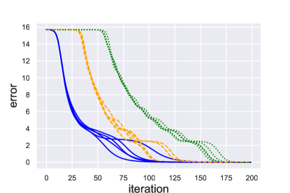
Figure 1: Convergence of gradient descent with different magnitude of initialization: $\alpha=0.5$ (blue, solid), $\alpha=0.5d^{-1}$ (orange, dashed), and $\alpha=0.5d^{-2}$ (green, dotted).

6.2 Asymmetric matrix approximation

Our second experiment focuses on the asymmetric matrix approximation problem. We investigate the convergence of gradient descent when solving the regularized problem (5.1) or the following unregularized problem:

$$\bm{X}^{*},\bm{Y}^{*}=\mathop{\mathrm{argmin}}_{\bm{X}\in\mathbb{R}^{d_{1}\times r},\bm{Y}\in\mathbb{R}^{d_{2}\times r}}f_{\rm unreg}(\bm{X},\bm{Y})=\frac{1}{2}\|\bm{\Sigma}-\bm{X}\bm{Y}^{\top}\|_{{\scriptstyle\mathrm{F}}}^{2}.$$ (6.1)

Specifically, when solving problem (6.1), the gradient descent algorithm proceeds as follows:

$$\bm{X}_{t+1} =\bm{X}_{t}+\eta(\bm{\Sigma}-\bm{X}_{t}\bm{Y}_{t}^{\top})\bm{Y}_{t},$$

$$\bm{Y}_{t+1} =\bm{Y}_{t}+\eta(\bm{\Sigma}-\bm{X}_{t}\bm{Y}_{t}^{\top})^{\top}\bm{X}_{t},$$

where $(\bm{X}_{0},\bm{Y}_{0})\in\mathbb{R}^{d_{1}\times r}\times\mathbb{R}^{d_{2}\times r}$ represents the initialization point and $\eta$ is the learning rate. We aim to study the effects of the balancing regularizer by comparing the convergence behaviors of gradient descent in solving the regularized problem (5.1) and the unregularized problem (6.1).

In the experiment, we adopt the same values of $d$, $r$, and $\bm{\Sigma}$ as in the previous subsection. For both the regularized problem and the unregularized problem, we initialize $(\bm{X}_{0},\bm{Y}_{0})=\alpha(\bm{N}_{0},\bm{N}_{1})$, where $\bm{N}_{0}\in\mathbb{R}^{d\times r}$ and $\bm{N}_{1}\in\mathbb{R}^{d\times r}$ have i.i.d. entries following $\mathcal{N}(0,1/d)$. We consider two types of initialization magnitudes: $\alpha=1/d$ and $\alpha=4$. For each algorithm, we set the learning rate $\eta=0.05$, compute $(\bm{X}_{t},\bm{Y}_{t})$ for each iteration, and report the error $\|\bm{\Sigma}_{r}-\bm{X}_{t}\bm{Y}_{t}^{\top}\|_{{\scriptstyle\mathrm{F}}}$. We repeat the experiment five times for each algorithm and display the results in Figure 2.

As shown in the results, when using relatively small random initialization ($\alpha=1/d$), both the regularized and unregularized methods perform efficiently. However, with moderate random initialization ($\alpha=4$), the regularized method achieves faster convergence compared to the unregularized method. This improvement can be attributed to the balancing regularizer, which promotes more balanced iterations $(\bm{X}_{t},\bm{Y}_{t})$, ultimately contributing to improved convergence.

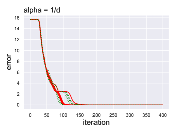
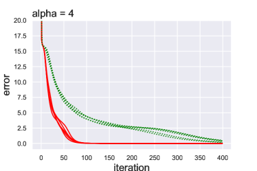
Figure 2: Comparison between the regularized (red, solid) and the unregularized (green, dotted) approaches for solving the asymmetric matrix approximation problems.

6.3 Retraction-free eigenspace computation

In this subsection, we numerically demonstrate the effectiveness of the retraction-free eigenspace computation method. We solve the eigenspace computation problems using both the Riemannian gradient descent (RGD) method (5.4) and (5.5), and the retraction-free method (5.6), and then compare the results. We consider the following settings: (A) $d=500$, $r=10$, and $\bm{\Sigma}={\rm diag}(7,6.5,\ldots,2,\bm{I}_{d-r})\in\mathbb{R}^{d\times d}$; (B) $d=500$, $r=10$, and $\bm{\Sigma}={\rm diag}(3,\ldots,3,\bm{I}_{d-r})\in\mathbb{R}^{d\times d}$. In both settings, $\bm{\Pi}_{r}={\rm diag}(\bm{I}_{r},{\bm{0}})$. We initialize $\widetilde{\bm{L}}_{0}=\bm{N}_{0}$ for RGD and $\bm{L}_{0}=\bm{N}_{0}$ for the retraction-free algorithm, where $\bm{N}_{0}\in\mathbb{R}^{d\times r}$ has i.i.d. entries following $\mathcal{N}(0,1/d)$. We set the learning rate $\eta=0.05$, compute $\bm{L}_{t}$ using both methods, and report the error $\|\bm{\Pi}_{r}-\bm{L}_{t}\bm{L}_{t}^{\top}\|_{{\scriptstyle\mathrm{F}}}$. We repeat the experiment five times for each setting and display the results in Figure 3.

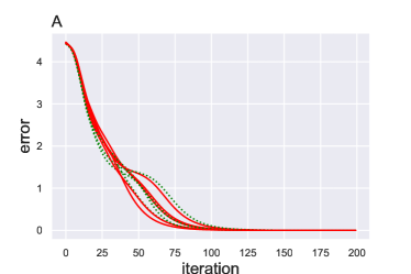
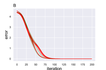
Figure 3: Comparison between RGD (green, dotted) and the retraction-free algorithm (red, solid).

As illustrated, $\bm{\Pi}_{r}-\bm{L}_{t}\bm{L}_{t}^{\top}$ converges rapidly to zero using both methods in both settings. This demonstrates that (1) both eigenspace computation methods are efficient, and (2) the retraction-free method is as efficient as the original RGD method in terms of the number of iterations.

To achieve the same precision, both RGD and the retraction-free algorithm require approximately the same number of iterations. However, since the retraction-free algorithm does not perform the retraction step (5.4), it is expected to be faster than RGD. To validate this claim, we compare the runtime performance between RGD and the retraction-free algorithm using setting (A) as the basis for our evaluation. We employ the same initialization mechanism as in the previous experiment. Let $\epsilon=0.0001$. We calculate the runtime needed for each algorithm to reach the precision level $\|\bm{\Pi}_{r}-\bm{L}_{t}\bm{L}_{t}^{\top}\|_{{\scriptstyle\mathrm{F}}}\leq\epsilon$. We repeat the experiment 200 times and report the total runtime for each algorithm in Table 1. The results demonstrate that the retraction-free algorithm is considerably more efficient than RGD, saving a total of 29.1% runtime.

Table 1: Comparison of the runtime performance between RGD and the retraction-free algorithm.

	RGD	retraction-free algorithm
Runtime	304.4s	215.7s

7 Related work

Low-rank matrix approximation (1.2) plays a significant role in statistics and engineering. In Section 5, we highlight the close relationship between this problem and the eigenspace computation problem, a connection also noted by Pitaval et al. (2015). Additionally, matrix approximation is relevant to a variety of low-rank optimization problems, such as matrix sensing (Ma et al., 2019; Zhu et al., 2021), phase retrieval (Chen et al., 2019), and matrix completion (Chen et al., 2020; Ma et al., 2019). These problems can be consolidated into the following optimization problem:

$$\bm{X}^{*}=\mathop{\mathrm{argmin}}_{\bm{X}\in\mathbb{R}^{d\times r}}\mathcal{L}(\bm{X}\bm{X}^{\top}),$$ (7.1)

where $\mathcal{L}(\cdot)$ represents a specific loss function depending on the problem at hand. The major challenge lies in the optimization properties for the algorithms in solving (7.1). Fortunately, despite its non-convex nature, many studies have demonstrated the effectiveness of gradient descent in solving problem (7.1) (Ma et al., 2019; Chen et al., 2019; Stöger and Soltanolkotabi, 2021). However, most of these works focus on the factorization problem, which corresponds to problem (1.2) with $\bm{\Sigma}$ having an exact rank of $r$. The sole exception is Chen et al. (2019), which only addresses the case of $r=1$. Consequently, the convergence rate of gradient descent in solving problem (1.2) with general $\bm{\Sigma}$ remains unknown, which is addressed by this paper.

The convergence analysis of gradient descent for problem (1.2) or (7.1) can be divided into two distinct stages: local convergence and warm-up. Most of the aforementioned studies concentrate on the local convergence stage, meaning that the algorithm is initialized within a benign region surrounding the global minimum. These studies do not address the issue of avoiding saddle points in the warm-up stage when a random initialization is utilized. To tackle the saddle point escaping problem, one line of research investigates the optimization landscape. They demonstrate that for problems including matrix sensing (Zhu et al., 2021), matrix completion (Ge et al., 2017), phase retrieval (Sun et al., 2018), dictionary learning (Sun et al., 2016), there are no spurious local minima, and all of the saddle points are strict, that is, the Hessian matrices evaluated at the saddle point has a negative eigenvalue. These geometric theories, in conjunction with the theory by Lee et al. (2019), imply that first-order algorithms almost surely converge to the global minimum. However, these arguments do not provide a convergence rate. In some cases, gradient descent may take exponential time to escape the saddle points (Du et al., 2017). To efficiently escape saddle points and converge to the global minimum in polynomial time, several saddle point escaping algorithms have been proposed, including perturbed gradient descent (Jin et al., 2017) and cubic regularization (Nesterov and Polyak, 2006). Nonetheless, these theories do not apply to the vanilla gradient descent algorithm.

Recent years have witnessed more research investigating the implicit regularization of vanilla gradient descent in solving matrix approximation problems (Li et al., 2018; Jiang et al., 2022; Stöger and Soltanolkotabi, 2021; Ye and Du, 2021). Stöger and Soltanolkotabi (2021) demonstrated that with small random initialization, gradient descent in solving matrix approximation problems behaves like a spectral method during the early iterations. Building on this observation, Jiang et al. (2022) studied the asymmetric matrix approximation problem and Jin et al. (2023) revealed the incremental learning of gradient descent in solving matrix sensing problems. In our paper, we combine this implicit regularization with our local convergence theory to demonstrate the fast global convergence of gradient descent with small random initialization. Furthermore, our paper suggests that small random initialization may not be necessary for fast global convergence. We demonstrate this statement in the special case where the top eigenvalues of $\bm{\Sigma}$ are identical, extending the rank-one result by Chen et al. (2019); Yi et al. (2005). For more general $\bm{\Sigma}$, we leave it to future research.

8 Discussion

This paper establishes the local linear convergence of gradient descent in solving the matrix approximation problem (1.2). A major novel technique employed is the analysis of the ratio $\sigma_{1}^{2}(\bm{J})/\sigma_{r}^{2}(\bm{U})$ in Lemma 2.3, which may be of independent interest. By combining this analysis with the implicit regularization effect of gradient descent with small random initialization, we prove the fast global convergence of gradient descent when such initialization is used. Furthermore, we conjecture that small initialization is not necessary for achieving fast global convergence, and we demonstrate this statement in the special case where the leading eigenvalues of $\bm{\Sigma}$ are identical. Our results are extended to the asymmetric matrix approximation problem, and we also apply our findings to validate the effectiveness of a retraction-free eigenspace computation method. The results of our numerical experiments provide strong support for our theoretical findings. Finally, we point out the following topics for future research:

• Investigating the conjecture: exploring whether gradient descent (1.3) achieves rapid global convergence even with moderate random initialization.

• Examining the retraction-free eigenspace computation method in a streaming setting (Shamir, 2016; Tang, 2019).

Appendix

In Appendix A, we demonstrate the local linear convergence of gradient descent (1.3). Appendix B establishes the fast global convergence with small random initialization. Appendix C provides the proof for the fast global convergence when utilizing moderate random initialization. Appendix D proves all corollaries in Section 5.

Appendix A Proof of Section 2: local linear convergence

We prove Lemma 2.2 in Section A.1. In Section A.2, we provide the proof for Lemma 2.3 and in Section A.3, we demonstrate Lemma 2.4.

A.1 Proof of Lemma 2.2

Proof.

We prove this lemma by induction. Suppose $\bm{X}_{t}\in\mathcal{R}$. By Lemma A.1, since $\sigma_{1}^{2}(\bm{X}_{t})\leq 2\lambda_{1}^{*}$, we have $\sigma_{1}^{2}(\bm{X}_{t+1})\leq 2\lambda_{1}^{*}$. By Lemma A.2, since $\sigma_{1}^{2}(\bm{X}_{t})\leq 2\lambda_{1}^{*}$ and $\sigma_{1}^{2}(\bm{J}_{t})\leq\lambda_{r}^{*}-\Delta/2$, we have $\sigma_{1}^{2}(\bm{J}_{t+1})\leq\lambda_{r}^{*}-\Delta/2$. Finally, by Lemma A.3, since $\bm{X}_{t}\in\mathcal{R}$, we have $\sigma_{r}^{2}(\bm{U}_{t+1})\geq\Delta/4$ and thus $\bm{X}_{t+1}\in\mathcal{R}$. By induction, we conclude that $\bm{X}_{t^{\prime}}\in\mathcal{R}$ for all $t^{\prime}\geq t.$ ∎

A.1.1 Technical lemmas

We summarize technical lemmas used in the proof of Lemma 2.2. Lemma A.1 shows that ${\mathcal{S}}_{1}=\{\bm{X}\in\mathbb{R}^{d\times r}\mid\sigma_{1}(\bm{X})\leq a\}$ is an absorbing set of gradient descent for any $a\in[\sqrt{\lambda_{1}^{*}},1/\sqrt{3\eta}]$. In other words, once $\bm{X}_{t}$ enters ${\mathcal{S}}_{1}$, it will remain in it.

Lemma A.1.

Suppose $\eta\leq\frac{1}{3\lambda_{1}^{*}}$. For any $a\in[\sqrt{\lambda_{1}^{*}},1/\sqrt{3\eta}]$, if $\sigma_{1}(\bm{X}_{t})\leq a$, then $\sigma_{1}(\bm{X}_{t^{\prime}})\leq a$ for all $t^{\prime}\geq t$.

Proof.

Lemma A.4 states that if $\sigma_{1}(\bm{X}_{t})\leq 1/\sqrt{3\eta}$, then the following inequality holds

$$\sigma_{1}(\bm{X}_{t+1})\leq(1+\eta\lambda_{1}^{*}-\eta\sigma_{1}^{2}(\bm{X}_{t}))\cdot\sigma_{1}(\bm{X}_{t}).$$

When $\sqrt{\lambda_{1}^{*}}\leq\sigma_{1}(\bm{X}_{t})\leq a$, the inequality above implies that $\sigma_{1}(\bm{X}_{t+1})\leq\sigma_{1}(\bm{X}_{t})\leq a$. If $\sigma_{1}(\bm{X}_{t})\leq\sqrt{\lambda_{1}^{*}}\leq a$, then considering that $g_{1}(s)=(1+\eta\lambda_{1}^{*}-\eta s^{2})s$ is increasing on $[0,1/\sqrt{3\eta}]$, we obtain

$$\sigma_{1}(\bm{X}_{t+1})\leq(1+\eta\lambda_{1}^{*}-\eta\lambda_{1}^{*})\sqrt{\lambda_{1}^{*}}\leq a.$$

Hence, $\sigma_{1}(\bm{X}_{t+1})\leq a$. By induction, it follows that $\sigma_{1}(\bm{X}_{t^{\prime}})\leq a$ for all $t^{\prime}\geq t$. ∎

Lemma A.2 demonstrates that if $\sigma_{1}(\bm{X}_{t})\leq\sqrt{2\lambda_{1}^{*}}$ and $\sigma_{1}^{2}(\bm{J}_{t})\leq a$ for any $a\geq\lambda_{r+1}^{*}$, then $\sigma_{1}^{2}(\bm{J}_{t+1})\leq a$. By induction and Lemma A.1, this implies that ${\mathcal{S}}_{2}=\{\bm{X}=(\bm{U}^{\top}\bm{J}^{\top})^{\top}\in\mathbb{R}^{d\times r}\mid\sigma_{1}(\bm{X})\leq\sqrt{2\lambda_{1}^{*}},\sigma_{1}^{2}(\bm{J})\leq a\}$ is an absorbing set of gradient descent, provided that $a\geq\lambda_{r+1}^{*}$ and $\eta\leq\frac{1}{12\lambda_{1}^{*}}$. In other words, if $\bm{X}_{t}$ enters ${\mathcal{S}}_{2}$, then $\bm{X}_{t}$ will remain in ${\mathcal{S}}_{2}$ afterwards.

Lemma A.2.

Suppose $\eta\leq\frac{1}{12\lambda_{1}^{*}}$ and $\sigma_{1}(\bm{X}_{t})\leq\sqrt{2\lambda_{1}^{*}}$. For any $a\geq\lambda_{r+1}^{*}$, if $\sigma_{1}^{2}(\bm{J}_{t})\leq a$, then $\sigma_{1}^{2}(\bm{J}_{t+1})\leq a$.

Proof.

By Lemma A.5, we have

$$\sigma_{1}(\bm{J}_{t+1})\leq(1+\eta(\lambda_{r+1}^{*}-\sigma_{1}^{2}(\bm{J}_{t})))\cdot\sigma_{1}(\bm{J}_{t}).$$

If $\lambda_{r+1}^{*}<\sigma_{1}^{2}(\bm{J}_{t})\leq a$, then this inequality implies that $\sigma_{1}^{2}(\bm{J}_{t+1})\leq\sigma_{1}^{2}(\bm{J}_{t})\leq a$. If $\sigma_{1}^{2}(\bm{J}_{t})\leq\lambda_{r+1}^{*}\leq a$, then the observation that $g_{2}(s)=(1+\eta(\lambda_{r+1}^{*}-s^{2}))s$ is increasing on $[0,1/\sqrt{3\eta}]$ gives that

$$\sigma_{1}^{2}(\bm{J}_{t+1})\leq(1+\eta(\lambda_{r+1}^{*}-\lambda_{r+1}^{*}))^{2}\lambda_{r+1}^{*}\leq a,$$

which concludes the proof. ∎

Lemma A.3 is the last piece needed to show that region $\mathcal{R}$ is an absorbing set of gradient descent.

Lemma A.3.

Suppose $\eta\leq\frac{\Delta^{2}}{32\lambda_{1}^{*3}}$, $\sigma_{1}(\bm{X}_{t})\leq\sqrt{2\lambda_{1}^{*}}$, $\sigma_{1}^{2}(\bm{J}_{t})\leq\lambda_{r}^{*}-\Delta/2$. If $\sigma_{r}^{2}(\bm{U}_{t})\geq\Delta/4$, then $\sigma_{r}^{2}(\bm{U}_{t+1})\geq\Delta/4$.

Proof.

Since $\eta\leq\frac{1}{32\lambda_{1}^{*}}$ and $\sigma_{1}^{2}(\bm{J}_{t})\leq\lambda_{r}^{*}-\Delta/2$, by Lemma A.6, we have

$$\sigma_{r}^{2}(\bm{U}_{t+1})\geq(1+\eta\Delta-2\eta\sigma_{r}^{2}(\bm{U}_{t}))\sigma_{r}^{2}(\bm{U}_{t})-4\eta^{2}\lambda_{1}^{*3}.$$

Since the function $g_{3}(s)=(1+\eta\Delta-2\eta s)s$ is increasing on $(-\infty,\frac{1}{4\eta}]$ and $\Delta/4\leq\sigma_{r}^{2}(\bm{U}_{t})\leq 2\lambda_{1}^{*}\leq 1/4\eta$, we have

$$\sigma_{r}^{2}(\bm{U}_{t+1}) \geq(1+\eta\Delta/2)\Delta/4-4\eta^{2}\lambda_{1}^{*3}$$

$$\geq\Delta/4,$$

where the last inequality follows from $\eta\leq\frac{\Delta^{2}}{32\lambda_{1}^{*3}}$. ∎

The following three lemmas provide bounds for singular value. Lemma A.4 establishes an upper bound for $\sigma_{1}(\bm{X}_{t+1})$, Lemma A.5 gives an upper bound for $\sigma_{1}(\bm{J}_{t+1})$, and Lemma A.6 provides an lower bound for $\sigma_{r}^{2}(\bm{U}_{t+1})$ in terms of the previous iteration.

Lemma A.4.

If $\sigma_{1}(\bm{X}_{t})\leq 1/\sqrt{3\eta}$, then we have

$$\sigma_{1}(\bm{X}_{t+1})\leq(1+\eta\lambda_{1}^{*}-\eta\sigma_{1}^{2}(\bm{X}_{t}))\cdot\sigma_{1}(\bm{X}_{t}).$$

Proof.

By the singular value inequality and (1.3),

$$\sigma_{1}(\bm{X}_{t+1}) \leq\sigma_{1}(\bm{X}_{t}(\bm{I}_{r}-\eta\bm{X}_{t}^{\top}\bm{X}_{t}))+\eta\sigma_{1}(\bm{\Sigma}\bm{X}_{t})$$

$$\leq\sigma_{1}(\bm{X}_{t}(\bm{I}_{r}-\eta\bm{X}_{t}^{\top}\bm{X}_{t}))+\eta\lambda_{1}^{*}\sigma_{1}(\bm{X}_{t}),$$ (A.1)

where we use $\sigma_{1}(\bm{\Sigma})=\lambda_{1}^{*}$. Observe that all $r$ singular values of $\bm{X}_{t}(\bm{I}_{r}-\eta\bm{X}_{t}^{\top}\bm{X}_{t})$ are given by

$$(1-\eta\sigma_{i}^{2}(\bm{X}_{t}))\cdot\sigma_{i}(\bm{X}_{t}),\ i=1,\ldots,r,$$

since $\eta\sigma_{1}^{2}(\bm{X}_{t})\leq 1$. Since $g_{4}(s)=(1-\eta s^{2})s$ is increasing on $[0,1/\sqrt{3\eta}]$, and $0\leq\sigma_{i}(\bm{X}_{t})\leq\sigma_{1}(\bm{X}_{t})\leq 1/\sqrt{3\eta}$, we get

$$\sigma_{1}(\bm{X}_{t}(\bm{I}_{r}-\eta\bm{X}_{t}^{\top}\bm{X}_{t}))=(1-\eta\sigma_{1}^{2}(\bm{X}_{t}))\cdot\sigma_{1}(\bm{X}_{t}).$$

Substituting this equality into (A.1), we conclude the proof. ∎

Lemma A.5.

Suppose $\eta\leq\frac{1}{12\lambda_{1}^{*}}$ and $\sigma_{1}(\bm{X}_{t})\leq\sqrt{2\lambda_{1}^{*}}$, then we have

$$\sigma_{1}(\bm{J}_{t+1})\leq(1+\eta(\lambda_{r+1}^{*}-\sigma_{1}^{2}(\bm{J}_{t})-\sigma_{r}^{2}(\bm{U}_{t})))\cdot\sigma_{1}(\bm{J}_{t}).$$

Proof.

The update rule (2.2) can be decomposed as follows:

$$\bm{J}_{t+1}=\underbrace{\frac{1}{2}\bm{J}_{t}-\eta\bm{J}_{t}\bm{J}_{t}^{\top}\bm{J}_{t}}_{\bm{B}}+\underbrace{(\frac{1}{4}\bm{I}_{d-r}+\eta\bm{\Lambda}_{\rm res})\bm{J}_{t}}_{\bm{C}}+\underbrace{\bm{J}_{t}(\frac{1}{4}\bm{I}_{r}-\eta\bm{U}_{t}^{\top}\bm{U}_{t})}_{\bm{D}}.$$

By the singular value inequality,

$$\sigma_{1}(\bm{J}_{t+1})\leq\sigma_{1}(\bm{B})+\sigma_{1}(\bm{C})+\sigma_{1}(\bm{D}).$$

Observe that all singular values of $\bm{B}$ are given by

$$\sigma_{i}(\bm{J}_{t})/2-\eta\sigma_{i}^{3}(\bm{J}_{t}),\quad i=1,\ldots,d-r.$$

Since $g_{5}(s)=s/2-\eta s^{3}$ is increasing on $[0,1/\sqrt{6\eta}]$, the condition $\sigma_{i}(\bm{J}_{t})\leq\sigma_{1}(\bm{J}_{t})\leq\sqrt{2\lambda_{1}^{*}}\leq 1/\sqrt{6\eta}$ implies that

$$\sigma_{1}(\bm{B})=\sigma_{1}(\bm{J}_{t})/2-\eta\sigma_{1}^{3}(\bm{J}_{t}).$$

For the second term $\bm{C}$, it follows from the singular value inequality that

$$\sigma_{1}(\bm{C})\leq\sigma_{1}(\frac{1}{4}\bm{I}_{d-r}+\eta\bm{\Lambda}_{\rm res})\sigma_{1}(\bm{J}_{t})\leq(1/4+\eta\lambda_{r+1}^{*})\sigma_{1}(\bm{J}_{t}),$$

where the second inequality uses $\eta\sigma_{1}(\bm{\Lambda}_{\rm res})\leq\eta\lambda_{1}^{*}\leq 1/4.$ For the third term $\bm{D}$, since $\eta\sigma_{1}^{2}(\bm{U}_{t})\leq 2\eta\lambda_{1}^{*}\leq 1/4$,

$$\sigma_{1}(\bm{D})\leq(1/4-\eta\sigma_{r}^{2}(\bm{U}_{t}))\sigma_{1}(\bm{J}_{t}).$$

Finally, we conclude the proof by combining the analysis of $\bm{B},\bm{C},$ and $\bm{D}$. ∎

Lemma A.6.

Suppose $\eta\leq\frac{1}{32\lambda_{1}^{*}}$ and $\sigma_{1}(\bm{X}_{t})\leq\sqrt{2\lambda_{1}^{*}}$, then we have

$$\sigma_{r}^{2}(\bm{U}_{t+1})\geq(1+2\eta(\lambda_{r}^{*}-\sigma_{1}^{2}(\bm{J}_{t})-\sigma_{r}^{2}(\bm{U}_{t})))\cdot\sigma_{r}^{2}(\bm{U}_{t})-4\eta^{2}\lambda_{1}^{*3}.$$

Proof.

Substituting the update rule (2.1) into $\bm{U}_{t+1}\bm{U}_{t+1}^{\top}$ and we get

$$\bm{U}_{t+1}\bm{U}_{t+1}^{\top} =(\bm{U}_{t}-\eta\bm{U}_{t}\bm{X}_{t}^{\top}\bm{X}_{t}+\eta\bm{\Lambda}_{r}\bm{U}_{t})\cdot(\bm{U}_{t}-\eta\bm{U}_{t}\bm{X}_{t}^{\top}\bm{X}_{t}+\eta\bm{\Lambda}_{r}\bm{U}_{t})^{\top}$$

$$=\bm{B}+\bm{C}-\eta^{2}\bm{R}_{1}+\eta^{2}\bm{R}$$

where

$$\bm{B} =\bm{U}_{t}(\frac{1}{2}\bm{I}_{r}-2\eta\bm{X}_{t}^{\top}\bm{X}_{t})\bm{U}_{t}^{\top},$$

$$\bm{C} =(\frac{1}{\sqrt{2}}\bm{I}_{r}+\sqrt{2}\eta\bm{\Lambda}_{r})\bm{U}_{t}\bm{U}_{t}^{\top}(\frac{1}{\sqrt{2}}\bm{I}_{r}+\sqrt{2}\eta\bm{\Lambda}_{r}),$$

$$\bm{R}_{1} =2\bm{\Lambda}_{r}\bm{U}_{t}\bm{U}_{t}^{\top}\bm{\Lambda}_{r},$$

$$\bm{R} =(\bm{\Lambda}_{r}\bm{U}_{t}-\bm{U}_{t}\bm{X}_{t}^{\top}\bm{X}_{t})(\bm{\Lambda}_{r}\bm{U}_{t}-\bm{U}_{t}\bm{X}_{t}^{\top}\bm{X}_{t})^{\top}.$$

Here $\bm{B}$ is positive semi-definite (PSD) since $2\eta\sigma_{1}^{2}(\bm{X}_{t})\leq 4\eta\lambda_{1}^{*}\leq 1/2$ and $\bm{C},\bm{R}_{1},\bm{R}$ are all PSD. By the eigenvalue inequality and the equivalence between eigenvalues and singular values of a PSD matrix, we have

$$\sigma_{r}^{2}(\bm{U}_{t+1}) \geq\sigma_{r}(\bm{B})+\sigma_{r}(\bm{C})-\eta^{2}\sigma_{1}(\bm{R}_{1})+\eta^{2}\sigma_{r}(\bm{R})$$

$$\geq\sigma_{r}(\bm{B})+\sigma_{r}(\bm{C})-\eta^{2}\sigma_{1}(\bm{R}_{1}).$$ (A.2)

For the first term $\bm{B}$, we decompose it into two terms:

$$\bm{B}=\underbrace{\bm{U}_{t}((\frac{1}{2}-2\eta\sigma_{1}^{2}(\bm{J}_{t}))\cdot\bm{I}_{r}-2\eta\bm{U}_{t}^{\top}\bm{U}_{t})\bm{U}_{t}^{\top}}_{\bm{B}_{1}}+2\eta\cdot\underbrace{\bm{U}_{t}(\sigma_{1}^{2}(\bm{J}_{t})\cdot\bm{I}_{r}-\bm{J}_{t}^{\top}\bm{J}_{t})\bm{U}_{t}^{\top}}_{\bm{B}_{2}}.$$

The inequality $2\eta(\sigma_{1}^{2}(\bm{J}_{t})+\sigma_{1}^{2}(\bm{U}_{t}))\leq 8\eta\lambda_{1}^{*}\leq 1/2$ implies that $\bm{B}_{1}$ is PSD. Since $\bm{B}_{2}$ is also PSD, we have $\sigma_{r}(\bm{B})\geq\sigma_{r}(\bm{B}_{1})$. To determine $\sigma_{r}(\bm{B}_{1})$, we write the singular values of $\bm{B}_{1}$ as

$$(\frac{1}{2}-2\eta\sigma_{1}^{2}(\bm{J}_{t}))\cdot\sigma_{i}^{2}(\bm{U}_{t})-2\eta\sigma_{i}^{4}(\bm{U}_{t}),\ i=1,\ldots,r.$$

Since $1/2-2\eta\sigma_{1}^{2}(\bm{J}_{t})\geq 1/4$, the function $g_{6}(s)=(1/2-2\eta\sigma_{1}^{2}(\bm{J}_{t}))s-2\eta s^{2}$ is increasing on $(-\infty,\frac{1}{16\eta}]$. Then the inequality $\sigma_{i}^{2}(\bm{U}_{t})\leq\sigma_{1}^{2}(\bm{U}_{t})\leq 2\lambda_{1}^{*}\leq\frac{1}{16\eta}$ implies that

$$\sigma_{r}(\bm{B}_{1})=(\frac{1}{2}-2\eta(\sigma_{1}^{2}(\bm{J}_{t})+\sigma_{r}^{2}(\bm{U}_{t})))\cdot\sigma_{r}^{2}(\bm{U}_{t}).$$

For the second term $\bm{C}$, we have

$$\sigma_{r}(\bm{C})\geq\sigma_{r}^{2}(\frac{1}{\sqrt{2}}\bm{I}_{r}+\sqrt{2}\eta\bm{\Lambda}_{r})\sigma_{r}^{2}(\bm{U}_{t})\geq(\frac{1}{2}+2\eta\lambda_{r}^{*})\sigma_{r}^{2}(\bm{U}_{t}).$$

For the third term $\bm{R}_{1}$, since $\sigma_{1}(\bm{X}_{t})\leq\sqrt{2\lambda_{1}^{*}}$, we have

$$\sigma_{1}(\bm{R}_{1})\leq 4\lambda_{1}^{*3}.$$

Finally, substituting the analysis of $\bm{B},\bm{C},\bm{R}_{1}$ into (A.2) gives the desired result. ∎

A.2 Proof of Lemma 2.3

Proof.

By Lemma 2.2, we have $\bm{X}_{t}\in\mathcal{R}$ for all $t\geq 0$. Then by Lemma A.5,

$$\sigma_{1}^{2}(\bm{J}_{t+1}) \leq(1+2\eta(\lambda_{r+1}^{*}-\sigma_{1}^{2}(\bm{J}_{t})-\sigma_{r}^{2}(\bm{U}_{t}))+16\eta^{2}\lambda_{1}^{*2})\cdot\sigma_{1}^{2}(\bm{J}_{t})$$

$$\leq(1-\eta\Delta/2+2\eta(\lambda_{r}^{*}-\Delta/2-\sigma_{1}^{2}(\bm{J}_{t})-\sigma_{r}^{2}(\bm{U}_{t})))\cdot\sigma_{1}^{2}(\bm{J}_{t}),$$

where the second inequality follows from $\eta\leq\frac{\Delta}{32\lambda_{1}^{*2}}$. By Lemma A.6,

$$\sigma_{r}^{2}(\bm{U}_{t+1}) \geq(1+\eta\Delta+2\eta(\lambda_{r}^{*}-\Delta/2-\sigma_{1}^{2}(\bm{J}_{t})-\sigma_{r}^{2}(\bm{U}_{t})))\cdot\sigma_{r}^{2}(\bm{U}_{t})-4\eta^{2}\lambda_{1}^{*3}$$

$$\geq(1+\eta\Delta/2+2\eta(\lambda_{r}^{*}-\Delta/2-\sigma_{1}^{2}(\bm{J}_{t})-\sigma_{r}^{2}(\bm{U}_{t})))\cdot\sigma_{r}^{2}(\bm{U}_{t}),$$

where we use $\sigma_{r}^{2}(\bm{U}_{t})\geq\Delta/4$ and $\eta\leq\frac{\Delta^{2}}{32\lambda_{1}^{*3}}$ in the second inequality. A combination of the above two inequalities gives that

$$\frac{\sigma_{1}^{2}(\bm{J}_{t+1})}{\sigma_{r}^{2}(\bm{U}_{t+1})}\leq\frac{1-\eta\Delta/2+2\eta(\lambda_{r}^{*}-\Delta/2-\sigma_{1}^{2}(\bm{J}_{t})-\sigma_{r}^{2}(\bm{U}_{t}))}{1+\eta\Delta/2+2\eta(\lambda_{r}^{*}-\Delta/2-\sigma_{1}^{2}(\bm{J}_{t})-\sigma_{r}^{2}(\bm{U}_{t}))}\cdot\frac{\sigma_{1}^{2}(\bm{J}_{t})}{\sigma_{r}^{2}(\bm{U}_{t})}.$$

Since the function $g_{7}(s)=\frac{1-\eta\Delta/2+s}{1+\eta\Delta/2+s}$ is increasing on $[-1/2,1/2]$, the condition $-1/2\leq 2\eta(\lambda_{r}^{*}-\Delta/2-\sigma_{1}^{2}(\bm{J}_{t})-\sigma_{r}^{2}(\bm{U}_{t}))\leq 1/2$ implies that

$$\frac{\sigma_{1}^{2}(\bm{J}_{t+1})}{\sigma_{r}^{2}(\bm{U}_{t+1})}\leq\frac{3/2-\eta\Delta/2}{3/2+\eta\Delta/2}\cdot\frac{\sigma_{1}^{2}(\bm{J}_{t})}{\sigma_{r}^{2}(\bm{U}_{t})}\leq(1-\eta\Delta/3)\cdot\frac{\sigma_{1}^{2}(\bm{J}_{t})}{\sigma_{r}^{2}(\bm{U}_{t})}.$$

By deduction, we have

$$\sigma_{1}^{2}(\bm{J}_{t}) \leq(1-\eta\Delta/3)^{t}\cdot\sigma_{r}^{2}(\bm{U}_{t})\frac{\sigma_{1}^{2}(\bm{J}_{0})}{\sigma_{r}^{2}(\bm{U}_{0})}\leq(1-\eta\Delta/3)^{t}\cdot\frac{8\lambda_{1}^{*2}}{\Delta},$$

where the second inequality follows from $\sigma_{r}^{2}(\bm{U}_{t})\leq 2\lambda_{1}^{*}$, $\sigma_{1}^{2}(\bm{J}_{0})\leq\lambda_{1}^{*}$, and $\sigma_{r}^{2}(\bm{U}_{0})\geq\Delta/4$. Therefore, for any $\epsilon>0$, it takes at most $T_{\bm{J}}^{\epsilon}=\mathcal{O}(\frac{3}{\eta\Delta}\log\frac{8\lambda_{1}^{*2}}{\epsilon\Delta})$ iterations to have $\sigma_{1}^{2}(\bm{J}_{t})\leq\epsilon$. ∎

A.3 Proof of Lemma 2.4

Proof.

By Lemma 2.2, $\bm{X}_{t}\in\mathcal{R}$ for all $t\geq 0$. Using the notation of $\bm{P}_{t}$, (2.1) can be rewritten as

$$\bm{U}_{t+1}=\bm{U}_{t}+\eta\bm{P}_{t}\bm{U}_{t}-\eta\bm{U}_{t}\bm{J}_{t}^{\top}\bm{J}_{t}.$$

By direct calculation, we have

$$\bm{P}_{t+1}=(\bm{I}_{r}-\eta\bm{U}_{t}\bm{U}_{t}^{\top})\bm{P}_{t}(\bm{I}_{r}-\eta\bm{U}_{t}\bm{U}_{t}^{\top})-\eta^{2}(\bm{P}_{t}\bm{U}_{t}\bm{U}_{t}^{\top}\bm{P}_{t}+\bm{U}_{t}\bm{U}_{t}^{\top}\bm{P}_{t}\bm{U}_{t}\bm{U}_{t}^{\top})+\bm{R}_{t},$$

where

$$\bm{R}_{t}=\eta(\bm{I}_{r}+\eta\bm{P}_{t})\bm{U}_{t}\bm{J}_{t}^{\top}\bm{J}_{t}\bm{U}_{t}^{\top}+\eta\bm{U}_{t}\bm{J}_{t}^{\top}\bm{J}_{t}\bm{U}_{t}^{\top}(\bm{I}_{r}+\eta\bm{P}_{t})-\eta^{2}\bm{U}_{t}(\bm{J}_{t}^{\top}\bm{J}_{t})^{2}\bm{U}_{t}^{\top}.$$

By the singular value inequality,

$$\sigma_{1}(\bm{P}_{t+1}) \leq((1-\eta\Delta/4)^{2}+8\eta^{2}\lambda_{1}^{*2})\cdot\sigma_{1}(\bm{P}_{t})+\sigma_{1}(\bm{R}_{t})$$

$$\leq(1-\eta\Delta/4)\cdot\sigma_{1}(\bm{P}_{t})+\sigma_{1}(\bm{R}_{t}),$$

where we use $\Delta/4\leq\sigma_{r}^{2}(\bm{U}_{t})\leq\sigma_{1}^{2}(\bm{U}_{t})\leq 2\lambda_{1}^{*}$ in the first inequality and $\eta\leq\frac{\Delta}{36\lambda_{1}^{*2}}$ in the second inequality. For the remainder term $\bm{R}_{t}$, by the singular value inequality and the condition $\eta\leq\frac{\Delta^{2}}{36\lambda_{1}^{*3}}$, we have

$$\sigma_{1}(\bm{R}_{t})\leq\sigma_{1}^{2}(\bm{J}_{t})\leq(1-\eta\Delta/3)^{t}\cdot\frac{8\lambda_{1}^{*2}}{\Delta},$$

where the last inequality follows from Lemma 2.3. Then by deduction, we have

$$\frac{\sigma_{1}(\bm{P}_{t+1})}{(1-\eta\Delta/4)^{t+1}} \leq\frac{\sigma_{1}(\bm{P}_{t})}{(1-\eta\Delta/4)^{t}}+\left(\frac{1-\eta\Delta/3}{1-\eta\Delta/4}\right)^{t}\frac{8\lambda_{1}^{*2}}{(1-\eta\Delta/4)\Delta}$$

$$\leq\sigma_{1}(\bm{P}_{0})+\sum_{i=1}^{t}\left(\frac{1-\eta\Delta/3}{1-\eta\Delta/4}\right)^{i}\frac{8\lambda_{1}^{*2}}{(1-\eta\Delta/4)\Delta}$$

$$\leq\sigma_{1}(\bm{P}_{0})+\frac{96\lambda_{1}^{*2}}{\eta\Delta^{2}}\leq\frac{100\lambda_{1}^{*2}}{\eta\Delta^{2}},$$

where the last inequality follows from $\sigma_{1}(\bm{P}_{0})\leq 2\lambda_{1}^{*}$. Therefore, it takes $T_{\bm{P}}^{\epsilon}=\mathcal{O}(\frac{4}{\eta\Delta}\log\frac{100\lambda_{1}^{*2}}{\eta\Delta^{2}\epsilon})$ iterations to achieve $\sigma_{1}(\bm{P}_{t})\leq\epsilon$. ∎

Appendix B Proof of Section 3: small random initialization

B.1 Proof of Lemma 3.1

Proof.

The proof is similar to that of Lemma 2.2. Suppose $\bm{X}_{t}\in\mathcal{R}_{2}$. By Lemma A.1 and Lemma A.2, we have $\bm{X}_{t+1}\in\mathcal{R}_{2}$. Thus we conclude the proof by induction. ∎

B.2 Proof of Theorem 3.2

The proof of Theorem 3.2 is composed of two parts. First, we introduce a deterministic condition on the initialization, and establish the corresponding convergence rate in Theorem B.2. Then, by verifying the conditions of Theorem B.2 when utilizing a small random initialization, we finish the proof of Theorem 3.2. To proceed, let us introduce the following condition on the initialization.

Condition B.1.

Assume $\sigma_{1}^{2}(\bm{X}_{0})\leq\lambda_{1}^{*}$, $\sigma_{1}^{2}(\bm{J}_{0})\leq\lambda_{r}^{*}-\Delta/2$, $\Delta/4>\sigma_{r}^{2}(\bm{U}_{0})>0$, and

$$\sigma_{1}^{2}(\bm{J}_{0})\leq c_{1}\cdot\sigma_{r}(\bm{U}_{0})^{1+\kappa},$$

where $c_{1}=\frac{\Delta^{1-\kappa/2}}{2^{3-\kappa}\sqrt{\lambda_{1}^{*}}}$ and $\kappa=\frac{\log(1+\eta\lambda_{r+1}^{*})}{\log(1+\eta(\lambda_{r}^{*}-\Delta/2))}$.

Under Condition B.1, we can demonstrate the fast global convergence of gradient descent as follows.

Theorem B.2.

Suppose $\eta\leq\frac{\Delta^{2}}{36\lambda_{1}^{*3}}$ and Condition B.1 holds. Then for any $\epsilon>0$, $\|\bm{\Sigma}_{r}-\bm{X}_{t}\bm{X}_{t}^{\top}\|_{{\scriptstyle\mathrm{F}}}\leq\epsilon$ after $T=\mathcal{O}(\frac{1}{\eta\Delta}\log\frac{\Delta}{4\sigma_{r}^{2}(\bm{U}_{0})}+\frac{6}{\eta\Delta}\log\frac{200r\lambda_{1}^{*2}}{\eta\Delta^{2}\epsilon})$ iterations.

Proof of Theorem B.2.

By Lemma A.1 and Lemma 2.2, we obtain $\sigma_{1}^{2}(\bm{X}_{t})\leq\lambda_{1}^{*}$ and $\sigma_{1}^{2}(\bm{J}_{t})\leq\lambda_{r}^{*}-\Delta/2$ for all $t\geq 0$. By Lemma A.5, we have

$$\sigma_{1}(\bm{J}_{t+1})\leq(1+\eta\lambda_{r+1}^{*})\cdot\sigma_{1}(\bm{J}_{t}),\quad\forall t\geq 0.$$ (B.1)

Let $T_{\textnormal{I}}^{\prime}=\frac{\log(\frac{\Delta}{4\sigma_{r}^{2}(\bm{U}_{0})})}{2\log(1+\eta(\lambda_{r}^{*}-\Delta/2))}.$ Then Condition B.1 implies that

$$(1+\eta\max\{0,\lambda_{r+1}^{*}\})^{T_{\textnormal{I}}^{\prime}}\cdot\sigma_{1}^{2}(\bm{J}_{0}) =\left(\frac{\Delta}{4\sigma_{r}^{2}(\bm{U}_{0})}\right)^{\kappa/2}\cdot\sigma_{1}^{2}(\bm{J}_{0})\leq\frac{\Delta}{8\sqrt{\lambda_{1}^{*}}}\cdot\sigma_{r}(\bm{U}_{0}),$$

where $\kappa=\frac{\log(1+\eta\max\{0,\lambda_{r+1}^{*}\})}{\log(1+\eta(\lambda_{r}^{*}-\Delta/2))}$. Thus, for any $t\leq T_{\textnormal{I}}^{\prime}$, we have

$$(1+\eta\lambda_{r+1}^{*})^{2t}\cdot\sigma_{1}^{2}(\bm{J}_{0}) \leq(1+\eta\max\{0,\lambda_{r+1}^{*}\})^{t}\cdot\frac{\Delta}{8\sqrt{\lambda_{1}^{*}}}\cdot\sigma_{r}(\bm{U}_{0})$$

$$\leq(1+\eta\lambda_{r}^{*}-\eta\Delta/2)^{t}\cdot\frac{\Delta}{8\sqrt{\lambda_{1}^{*}}}\cdot\sigma_{r}(\bm{U}_{0}),$$ (B.2)

where we use $\lambda_{r+1}^{*}\leq\max\{0,\lambda_{r+1}^{*}\}\leq\lambda_{r}^{*}-\Delta/2$.

Let $T_{\textnormal{I}}=\min\{t\geq 0\mid\sigma_{r}^{2}(\bm{U}_{t})\geq\Delta/4\}$. We claim that the following inequality holds:

$$\sigma_{r}(\bm{U}_{t+1})\geq(1+\eta\lambda_{r}^{*}-\eta\Delta/2)\cdot\sigma_{r}(\bm{U}_{t}),\quad\forall t<\min\{T_{\textnormal{I}},T_{\textnormal{I}}^{\prime}\}.$$ (B.3)

This can be proved by induction. First, we show that if (B.3) holds for all $0\leq t<u<\min\{T_{\textnormal{I}},T_{\textnormal{I}}^{\prime}\}$, then (B.3) also holds for $t=u$. To see this, we have

$$\sigma_{1}^{2}(\bm{J}_{u})\leq(1+\eta\lambda_{r+1}^{*})^{2u}\cdot\sigma_{1}^{2}(\bm{J}_{0})\leq\frac{\Delta}{8\sqrt{\lambda_{1}^{*}}}\cdot(1+\eta\lambda_{r}^{*}-\eta\Delta/2)^{u}\cdot\sigma_{r}(\bm{U}_{0})\leq\frac{\Delta}{8\sqrt{\lambda_{1}^{*}}}\cdot\sigma_{r}(\bm{U}_{u}),$$ (B.4)

where the first inequality follows from (B.1), the second inequality follows from (B.2) and $u<T_{\textnormal{I}}^{\prime}$, and the third inequality follows from (B.3) for all $t<u$. Since $u<T_{\textnormal{I}}$, we have $\sigma_{r}^{2}(\bm{U}_{u})<\Delta/4$ by definition. Then by Lemma B.3 and the singular value inequality, we obtain

$$\sigma_{r}(\bm{U}_{u+1}) \geq\sigma_{r}\left(\bm{U}_{u}+\eta(\bm{\Lambda}_{r}-\bm{U}_{u}\bm{U}_{u}^{\top})\bm{U}_{u}\right)-\eta\sigma_{1}(\bm{U}_{u}\bm{J}_{u}^{\top}\bm{J}_{u})$$

$$\geq(1-2\eta^{2}\sigma_{1}(\bm{\Lambda}_{r}\bm{U}_{u}\bm{U}_{u}^{\top}))(1+\eta\lambda_{r}^{*})\sigma_{r}(\bm{U}_{u})(1-\eta\sigma_{r}^{2}(\bm{U}_{u}))-\eta\sigma_{1}(\bm{U}_{u}\bm{J}_{u}^{\top}\bm{J}_{u})$$

$$\geq(1-2\eta^{2}\lambda_{1}^{*2})(1+\eta\lambda_{r}^{*})(1-\eta\Delta/4)\sigma_{r}(\bm{U}_{u})-\frac{\eta\Delta}{8}\sigma_{r}(\bm{U}_{u})$$

$$\geq(1+\eta\lambda_{r}^{*}-\eta\Delta/2)\cdot\sigma_{r}(\bm{U}_{u}),$$

where the third inequality uses $\sigma_{r}^{2}(\bm{U}_{u})<\Delta/4$ and (B.4) and the fourth inequality uses $\eta\leq\frac{\Delta^{2}}{36\lambda_{1}^{*3}}$. By the same argument, we can show that (B.3) also holds for $t=0$ if $T_{\textnormal{I}}>0$. Thus, we finish the proof of the claim and (B.3) holds for all $t<\min\{T_{\textnormal{I}},T_{\textnormal{I}}^{\prime}\}$.

We claim that $T_{\textnormal{I}}\leq T_{\textnormal{I}}^{\prime}$. Otherwise, if $T_{\textnormal{I}}>T_{\textnormal{I}}^{\prime}$, then by (B.3), we have

$$\sigma_{r}(\bm{U}_{T_{\textnormal{I}}^{\prime}})\geq(1+\eta\lambda_{r}^{*}-\eta\Delta/2)^{T_{\textnormal{I}}^{\prime}}\cdot\sigma_{r}(\bm{U}_{0})=\sqrt{\Delta/4},$$

which contradicts to the definition of $T_{\textnormal{I}}$. Therefore, after $T_{\textnormal{I}}$ iterations, $\bm{X}_{t}$ enters the region $\mathcal{R}$ defined in (2.3), and we can apply Theorem 2.1 to the subsequent iterations. In particular, let $T=T_{\textnormal{I}}+T_{\textnormal{II}}^{\epsilon}=\mathcal{O}(\frac{1}{\eta\Delta}\log\frac{\Delta}{4\sigma_{r}^{2}(\bm{U}_{0})}+\frac{6}{\eta\Delta}\log\frac{200r\lambda_{1}^{*2}}{\eta\Delta^{2}\epsilon})$, where we use $T_{\textnormal{I}}=\mathcal{O}(\frac{1}{\eta\Delta}\log\frac{\Delta}{4\sigma_{r}^{2}(\bm{U}_{0})})$. Then $\|\bm{\Sigma}_{r}-\bm{X}_{t}\bm{X}_{t}^{\top}\|_{{\scriptstyle\mathrm{F}}}\leq\epsilon$ for all $t\geq T$, which concludes the proof. ∎

Lemma B.3 (Lemma D.4 in Jiang et al. [2022]).

Let $\bm{U}$ be an $r\times r$ matrix and $\bm{\Lambda}_{r}={\rm diag}(\lambda_{1}^{*},\ldots,\lambda_{r}^{*})\in\mathbb{R}^{r\times r}$ be a diagonal matrix with $\lambda_{1}^{*}\geq\ldots\geq\lambda_{r}^{*}>0$. Suppose $\sigma_{1}(\bm{U})>0$, $\eta\sigma_{1}(\bm{\Lambda}_{r}-\bm{U}\bm{U}^{\top})\leq 1/2$, $\sigma_{1}(\bm{U})\leq 1/\sqrt{3\eta}$, $2\eta^{2}\sigma_{1}(\bm{\Lambda}_{r}\bm{U}\bm{U}^{\top})<1$, and

$$\widetilde{\bm{U}}=\bm{U}+\eta(\bm{\Lambda}_{r}-\bm{U}\bm{U}^{\top})\bm{U}.$$

Then we have $\sigma_{r}(\widetilde{\bm{U}})\geq(1-2\eta^{2}\sigma_{1}(\bm{\Lambda}_{r}\bm{U}\bm{U}^{\top}))(1+\eta\lambda_{r}^{*})\sigma_{r}(\bm{U})(1-\eta\sigma_{r}^{2}(\bm{U}))$.

Now we proceed to prove Theorem 3.2. The key is to verify conditions in Theorem B.2 using the following concentration results.

Lemma B.4 (Random initialization Rudelson and Vershynin [2009], Wainwright [2019]).

Suppose $\bm{X}_{0}=\alpha\bm{N}_{0}$ with entries of $\bm{N}_{0}\in\mathbb{R}^{d\times r}$ $\rm i.i.d.$ $\mathcal{N}(0,\frac{1}{d})$. Let $\bm{X}_{0}=(\bm{U}_{0}^{\top}\bm{J}_{0}^{\top})^{\top}$ with $\bm{U}_{0}\in\mathbb{R}^{r\times r}$ and $\bm{J}_{0}\in\mathbb{R}^{(d-r)\times r}$. Then with probability greater than $1-Cc_{3}-C\exp(-d/C)$, we have

$$\sigma_{1}^{2}(\bm{J}_{0}) \leq\sigma_{1}^{2}(\bm{X}_{0})\leq c_{2}\alpha^{2},$$

$$\sigma_{r}(\bm{U}_{0}) \geq c_{3}\alpha/\sqrt{dr}\geq c_{3}\alpha/d,$$

where $C,c_{2},c_{3}$ are constants independent of $d$ and $r$.

Proof of Theorem 3.2.

By Lemma B.4, we have with high probability,

$$\sigma_{1}^{2}(\bm{J}_{0})\leq\sigma_{1}^{2}(\bm{X}_{0})\leq c_{2}\alpha^{2},\quad\sigma_{r}(\bm{U}_{0})\geq c_{3}\alpha/d,$$

where $c_{2}$ and $c_{3}$ are constants independent of $d$. If the magnitude of initialization $\alpha=\alpha_{0}d^{-\frac{1+\kappa}{1-\kappa}}$ for some constant $\alpha_{0}\leq(\frac{c_{1}c_{3}^{1+\kappa}}{c_{2}})^{\frac{1}{1-\kappa}}$, then with high probability, $\sigma_{1}^{2}(\bm{X}_{0})\leq\lambda_{1}^{*}$, $\sigma_{1}^{2}(\bm{J}_{0})\leq\lambda_{r}^{*}-\Delta/2$, and

$$c_{1}\cdot\sigma_{r}(\bm{U}_{0})^{1+\kappa} \geq c_{1}\cdot(c_{3}\alpha_{0}d^{-\frac{2}{1-\kappa}})^{1+\kappa}\geq\frac{c_{1}c_{3}^{1+\kappa}}{\alpha_{0}^{1-\kappa}c_{2}}\cdot\sigma_{1}^{2}(\bm{J}_{0})\geq\sigma_{1}^{2}(\bm{J}_{0}),$$

This verifies Condition B.1 and by Theorem B.2, we prove the result. ∎

Appendix C Proof of Section 4: moderate random initialization

C.1 Proof of Lemma 4.1

Proof.

By Lemma 3.1, we have $\bm{X}_{t}\in\mathcal{R}_{2}$ for all $t\geq 0$. Since $\lambda_{1}^{*}=\ldots=\lambda_{r}^{*}$, we have

$$\bm{U}_{t+1}=\bm{U}_{t}+\eta\lambda_{r}^{*}\bm{U}_{t}-\eta\bm{U}_{t}\bm{X}_{t}^{\top}\bm{X}_{t}.$$

Substituting this into $\bm{U}_{t+1}\bm{U}_{t+1}^{\top}$, we obtain

$$\bm{U}_{t+1}\bm{U}_{t+1}^{\top} =\bm{U}_{t}\bm{U}_{t}^{\top}+2\eta\lambda_{r}^{*}\bm{U}_{t}\bm{U}_{t}^{\top}-2\eta\bm{U}_{t}\bm{X}_{t}^{\top}\bm{X}_{t}\bm{U}_{t}^{\top}+\eta^{2}\bm{R}$$

$$=\bm{B}+\bm{C}+\eta^{2}\bm{R},$$

where

$$\bm{B} =\bm{U}_{t}(\frac{1}{2}\bm{I}_{r}+2\eta\lambda_{r}^{*}\bm{I}_{r}-2\eta\bm{J}_{t}^{\top}\bm{J}_{t})\bm{U}_{t}^{\top},$$

$$\bm{C} =\frac{1}{2}\bm{U}_{t}\bm{U}_{t}^{\top}-2\eta(\bm{U}_{t}\bm{U}_{t}^{\top})^{2},$$

$$\bm{R} =(\lambda_{r}^{*}\bm{U}_{t}-\bm{U}_{t}\bm{X}_{t}^{\top}\bm{X}_{t})(\lambda_{r}^{*}\bm{U}_{t}-\bm{U}_{t}\bm{X}_{t}^{\top}\bm{X}_{t})^{\top}.$$

Here $\bm{B},\bm{C}$, and $\bm{R}$ are all positive semi-definite (PSD) matrices. Hence, by the eigenvalue inequality and the equivalence between eigenvalues and singular values of a PSD matrix, we conclude that

$$\sigma_{r}^{2}(\bm{U}_{t+1})\geq\sigma_{r}(\bm{B})+\sigma_{r}(\bm{C}).$$

For the term $\bm{B}$, we have

$$\sigma_{r}(\bm{B})\geq(\frac{1}{2}+2\eta\lambda_{r}^{*}-2\eta\sigma_{1}^{2}(\bm{J}_{t}))\cdot\sigma_{r}^{2}(\bm{U}_{t}).$$

For $\bm{C}$, we can write its singular value as follows:

$$\frac{1}{2}\sigma_{i}^{2}(\bm{U}_{t})-2\eta\sigma_{i}^{4}(\bm{U}_{t}),\quad i=1,\ldots,r.$$

Since the function $g_{8}(x)=\frac{1}{2}x-2\eta x^{2}$ is increasing on $[0,1/8\eta]$, the condition that $\sigma_{r}^{2}(\bm{U}_{t})\leq\sigma_{i}^{2}(\bm{U}_{t})\leq 1/8\eta$ implies that

$$\sigma_{r}(\bm{C})=\frac{1}{2}\sigma_{r}^{2}(\bm{U}_{t})-2\eta\sigma_{r}^{4}(\bm{U}_{t}).$$

Combining, we have

$$\sigma_{r}^{2}(\bm{U}_{t+1}) \geq(1+2\eta\lambda_{r}^{*}-2\eta\sigma_{1}^{2}(\bm{J}_{t})-2\eta\sigma_{r}^{2}(\bm{U}_{t}))\cdot\sigma_{r}^{2}(\bm{U}_{t})$$

$$\geq(1+\eta\Delta-2\eta\sigma_{r}^{2}(\bm{U}_{t}))\cdot\sigma_{r}^{2}(\bm{U}_{t}).$$

where the second inequality holds due to the inequality $\sigma_{1}^{2}(\bm{J}_{t})\leq\lambda_{r}^{*}-\Delta/2.$ Let $T_{\bm{U}}=\{t\mid\sigma_{r}^{2}(\bm{U}_{t})\geq\Delta/4\}$. For all $t<T_{\bm{U}}$, we have

$$\sigma_{r}^{2}(\bm{U}_{t+1})\geq(1+\eta\Delta/2)\sigma_{r}^{2}(\bm{U}_{t}).$$

Hence, $\sigma_{r}^{2}(\bm{U}_{t})\geq(1+\eta\Delta/2)^{t}\sigma_{r}^{2}(\bm{U}_{0})$ for all $t\leq T_{\bm{U}}$. This implies that $T_{\bm{U}}=\mathcal{O}(\frac{2}{\eta\Delta}\log\frac{\Delta}{4\sigma_{r}^{2}(\bm{U}_{0})})$, which concludes the proof. ∎

C.2 Proof of Theorem 4.2

Proof.

Using a standard concentration result, Lemma B.4, we find that $\sigma_{1}(\bm{X}_{0})\asymp\alpha$ and $\sigma_{r}(\bm{U}_{0})\gtrsim\alpha/d$ with high probability. When $\alpha$ is small, it is highly probable that $\bm{X}_{0}\in\mathcal{R}_{2}$. By Lemma 3.1, it holds that $\bm{X}_{t}\in\mathcal{R}_{2}$ for all $t\geq 0$. According to Lemma 4.1 and Lemma B.4, it takes $T_{\bm{U}}=\mathcal{O}(\max\{\log(d),\log(1/\alpha)\})$ iterations to achieve $\sigma_{r}^{2}(\bm{U}_{t})\geq\Delta/4$, which leads to $\bm{X}_{t}\in\mathcal{R}$ for all $t\geq T_{\bm{U}}$. Finally, by invoking Theorem 2.1, we conclude the proof of this theorem. ∎

Appendix D Proof of Section 5: extensions

D.1 Proof of Corollary 5.1

Proof.

Assume with loss of generality that $d_{1}=d_{2}=d$ and $\bm{\Sigma}={\rm diag}(\sigma_{1}^{*},\ldots,\sigma_{d}^{*})$ with $\lambda_{1}^{*}\geq\ldots\geq\lambda_{d}^{*}$. Define

$$\bm{W}_{t}=(\frac{\bm{X}_{t}^{\top}+\bm{Y}_{t}^{\top}}{\sqrt{2}}\ \frac{\bm{X}_{t}^{\top}-\bm{Y}_{t}^{\top}}{\sqrt{2}})^{\top}\in\mathbb{R}^{2d\times r}.$$

Then (5.2) and (5.3) can be rewritten as

$$\bm{W}_{t+1}=\bm{W}_{t}+\frac{\eta}{2}\widetilde{\bm{\Sigma}}\bm{W}_{t}-\frac{\eta}{2}\bm{W}_{t}\bm{W}_{t}^{\top}\bm{W}_{t},\quad\widetilde{\bm{\Sigma}}=\begin{bmatrix}2\bm{\Sigma}&{\bm{0}}\\ {\bm{0}}&-2\bm{\Sigma}\end{bmatrix}\in\mathbb{R}^{2d\times 2d}.$$

This is exactly (1.4) with $(\bm{\Sigma},\bm{X}_{t},\eta)$ replaced by $(\widetilde{\bm{\Sigma}},\bm{W}_{t},\eta/2)$. By applying a modified version of Theorem 3.2, we can assert that $\widetilde{\bm{\Sigma}}_{r}-\bm{W}_{t}\bm{W}_{t}^{\top}$ converges to zero at a linear rate, where $\widetilde{\bm{\Sigma}}_{r}={\rm diag}(2\sigma_{1}^{*},\ldots,2\sigma_{r}^{*},{\bm{0}})\in\mathbb{R}^{2d\times 2d}$. Let $\bm{X}_{t}=(\bm{U}_{t}^{\top}\bm{J}_{t}^{\top})^{\top}$ and $\bm{Y}_{t}=(\bm{V}_{t}^{\top}\bm{H}_{t}^{\top})^{\top}$ with $\bm{U}_{t},\bm{V}_{t}\in\mathbb{R}^{r\times r}$ and $\bm{J}_{t},\bm{H}_{t}\in\mathbb{R}^{(d-r)\times r}$. The convergence $\widetilde{\bm{\Sigma}}_{r}-\bm{W}_{t}\bm{W}_{t}^{\top}\to{\bm{0}}$ implies that

$$(\bm{U}_{t}+\bm{V}_{t})(\bm{U}_{t}+\bm{V}_{t})^{\top}\to 4\bm{\Lambda}_{r},\quad\bm{J}_{t},\bm{H}_{t},\bm{U}_{t}-\bm{V}_{t}\to{\bm{0}},$$

where $\bm{\Lambda}_{r}={\rm diag}(\sigma_{1}^{*},\ldots,\sigma_{r}^{*})$. This implies that $\bm{\Sigma}_{r}-\bm{X}_{t}\bm{Y}_{t}^{\top}\to{\bm{0}}$ and $\bm{X}_{t}^{\top}\bm{X}_{t}-\bm{Y}_{t}^{\top}\bm{Y}_{t}\to{\bm{0}}$. The convergence rate follows in the same way, and we prove the corollary. ∎

D.2 Proof of Corollary 5.2

Proof.

The key idea is to relate (5.6) to the gradient descent updates (1.3) for a related symmetric low-rank matrix approximation. Specifically, we let $\bm{X}_{t}=\bm{\Sigma}^{1/2}\bm{L}_{t}$. By (5.6), we have

$$\bm{X}_{t+1}=\bm{X}_{t}+\eta\bm{\Sigma}\bm{X}_{t}-\eta\bm{X}_{t}\bm{X}_{t}^{\top}\bm{X}_{t},$$ (D.1)

which is exactly (1.3). By Theorem 3.2, we know $\bm{X}_{t}\bm{X}_{t}^{\top}$ converges to $\bm{\Sigma}_{r}$ quickly. The remaining task is to use this result to show that $\bm{\Pi}_{r}-\bm{L}_{t}\bm{L}_{t}^{\top}$ converges to zero rapidly.

Without loss of generality, we assume $\bm{\Sigma}={\rm diag}(\lambda_{1}^{*},\ldots,\lambda_{d}^{*})$ and thus $\bm{\Pi}_{r}={\rm diag}(\bm{I}_{r},{\bm{0}})$. Let $\bm{L}_{t}=(\bm{V}_{t}^{\top}\bm{H}_{t}^{\top})^{\top}$ with $\bm{V}_{t}\in\mathbb{R}^{r\times r}$ and $\bm{H}_{t}\in\mathbb{R}^{(d-r)\times r}$. Our aim is to show that both $\bm{I}_{r}-\bm{V}_{t}\bm{V}_{t}^{\top}$ and $\bm{H}_{t}$ converge fast to zero.

Let $\bm{\Lambda}_{r}={\rm diag}(\lambda_{1}^{*},\ldots,\lambda_{r}^{*})$, $\bm{\Lambda}_{\rm res}={\rm diag}(\lambda_{r+1}^{*},\ldots,\lambda_{d}^{*})$, and $\bm{X}_{t}=(\bm{U}_{t}^{\top}\bm{J}_{t}^{\top})^{\top}$ with $\bm{U}_{t}\in\mathbb{R}^{r\times r}$ and $\bm{J}_{t}\in\mathbb{R}^{(d-r)\times r}$. Then the fact that $\bm{X}_{t}\bm{X}_{t}^{\top}$ converges fast to $\bm{\Sigma}_{r}$ implies that both $\bm{\Lambda}_{r}-\bm{U}_{t}\bm{U}_{t}^{\top}$ and $\bm{J}_{t}$ converges quickly to zero.

By the rapid convergence of $\bm{\Lambda}_{r}-\bm{U}_{t}\bm{U}_{t}^{\top}\to{\bm{0}}$ and the equality $\bm{U}_{t}=\bm{\Lambda}_{r}^{1/2}\bm{V}_{t}$, we know $\bm{I}_{r}-\bm{V}_{t}\bm{V}_{t}^{\top}$ converges quickly to zero. Since $\bm{\Sigma}_{r}-\bm{X}_{t}\bm{X}_{t}^{\top}$ converges fast to zero, we have $\sigma_{r}^{2}(\bm{X}_{t})\geq(\lambda_{r}^{*}+\lambda_{r+1}^{*})/2$ for all $t\geq t_{0}$ and some small constant $t_{0}$. By (5.6), we have

$$\bm{H}_{t+1} =\bm{H}_{t}+\eta\bm{\Lambda}_{\rm res}\bm{H}_{t}-\eta\bm{H}_{t}\bm{X}_{t}^{\top}\bm{X}_{t}.$$

By the singular value inequality,

$$\sigma_{1}(\bm{H}_{t+1})\leq(1+\eta\lambda_{r+1}^{*}-\eta\sigma_{r}^{2}(\bm{X}_{t}))\cdot\sigma_{1}(\bm{H}_{t})\leq(1-\eta\Delta/2)\cdot\sigma_{1}(\bm{H}_{t}),\quad\forall t\geq t_{0}.$$

Hence, $\sigma_{1}(\bm{H}_{t})\leq(1-\eta\Delta/2)^{t-t_{0}}\sigma_{1}(\bm{H}_{t_{0}})$ for all $t\geq t_{0}$. This concludes the proof. ∎

References

- Burer and Monteiro (2003) Samuel Burer and Renato DC Monteiro. A nonlinear programming algorithm for solving semidefinite programs via low-rank factorization. Mathematical Programming, 95(2):329–357, 2003.
- Burer and Monteiro (2005) Samuel Burer and Renato DC Monteiro. Local minima and convergence in low-rank semidefinite programming. Mathematical programming, 103(3):427–444, 2005.
- Chen et al. (2020) Ji Chen, Dekai Liu, and Xiaodong Li. Nonconvex rectangular matrix completion via gradient descent without regularization. IEEE Transactions on Information Theory, 66(9):5806–5841, 2020.
- Chen et al. (2019) Yuxin Chen, Yuejie Chi, Jianqing Fan, and Cong Ma. Gradient descent with random initialization: Fast global convergence for nonconvex phase retrieval. Mathematical Programming, 176(1):5–37, 2019.
- Ding et al. (2021) Qinghua Ding, Kaiwen Zhou, and James Cheng. Tight convergence rate of gradient descent for eigenvalue computation. In Proceedings of the Twenty-Ninth International Conference on International Joint Conferences on Artificial Intelligence, pages 3276–3282, 2021.
- Du et al. (2017) Simon S Du, Chi Jin, Jason D Lee, Michael I Jordan, Aarti Singh, and Barnabas Poczos. Gradient descent can take exponential time to escape saddle points. Advances in neural information processing systems, 30, 2017.
- Ge et al. (2017) Rong Ge, Chi Jin, and Yi Zheng. No spurious local minima in nonconvex low rank problems: A unified geometric analysis. In International Conference on Machine Learning, pages 1233–1242. PMLR, 2017.
- Jiang et al. (2022) Liwei Jiang, Yudong Chen, and Lijun Ding. Algorithmic regularization in model-free overparametrized asymmetric matrix factorization. arXiv preprint arXiv:2203.02839, 2022.
- Jin et al. (2017) Chi Jin, Rong Ge, Praneeth Netrapalli, Sham M Kakade, and Michael I Jordan. How to escape saddle points efficiently. In International Conference on Machine Learning, pages 1724–1732. PMLR, 2017.
- Jin et al. (2023) Jikai Jin, Zhiyuan Li, Kaifeng Lyu, Simon S Du, and Jason D Lee. Understanding incremental learning of gradient descent: A fine-grained analysis of matrix sensing. arXiv preprint arXiv:2301.11500, 2023.
- Lee et al. (2019) Jason D Lee, Ioannis Panageas, Georgios Piliouras, Max Simchowitz, Michael I Jordan, and Benjamin Recht. First-order methods almost always avoid strict saddle points. Mathematical programming, 176(1):311–337, 2019.
- Li et al. (2018) Yuanzhi Li, Tengyu Ma, and Hongyang Zhang. Algorithmic regularization in over-parameterized matrix sensing and neural networks with quadratic activations. In Conference On Learning Theory, pages 2–47. PMLR, 2018.
- Ma et al. (2019) Cong Ma, Kaizheng Wang, Yuejie Chi, and Yuxin Chen. Implicit regularization in nonconvex statistical estimation: Gradient descent converges linearly for phase retrieval, matrix completion, and blind deconvolution. Foundations of Computational Mathematics, 2019.
- Nesterov and Polyak (2006) Yurii Nesterov and Boris T Polyak. Cubic regularization of newton method and its global performance. Mathematical Programming, 108(1):177–205, 2006.
- Pitaval et al. (2015) Renaud-Alexandre Pitaval, Wei Dai, and Olav Tirkkonen. Convergence of gradient descent for low-rank matrix approximation. IEEE Transactions on Information Theory, 61(8):4451–4457, 2015.
- Rudelson and Vershynin (2009) Mark Rudelson and Roman Vershynin. Smallest singular value of a random rectangular matrix. Communications on Pure and Applied Mathematics: A Journal Issued by the Courant Institute of Mathematical Sciences, 62(12):1707–1739, 2009.
- Shamir (2016) Ohad Shamir. Fast stochastic algorithms for svd and pca: Convergence properties and convexity. In International Conference on Machine Learning, pages 248–256. PMLR, 2016.
- Stöger and Soltanolkotabi (2021) Dominik Stöger and Mahdi Soltanolkotabi. Small random initialization is akin to spectral learning: Optimization and generalization guarantees for overparameterized low-rank matrix reconstruction. Advances in Neural Information Processing Systems, 34:23831–23843, 2021.
- Sun et al. (2016) Ju Sun, Qing Qu, and John Wright. Complete dictionary recovery over the sphere i: Overview and the geometric picture. IEEE Transactions on Information Theory, 63(2):853–884, 2016.
- Sun et al. (2018) Ju Sun, Qing Qu, and John Wright. A geometric analysis of phase retrieval. Foundations of Computational Mathematics, 18(5):1131–1198, 2018.
- Tang (2019) Cheng Tang. Exponentially convergent stochastic k-pca without variance reduction. Advances in Neural Information Processing Systems, 32, 2019.
- Wainwright (2019) Martin J Wainwright. High-dimensional statistics: A non-asymptotic viewpoint, volume 48. Cambridge University Press, 2019.
- Xu and Li (2021) Zhiqiang Xu and Ping Li. A comprehensively tight analysis of gradient descent for pca. Advances in Neural Information Processing Systems, 34:21935–21946, 2021.
- Ye and Du (2021) Tian Ye and Simon S Du. Global convergence of gradient descent for asymmetric low-rank matrix factorization. Advances in Neural Information Processing Systems, 34:1429–1439, 2021.
- Yi et al. (2005) Zhang Yi, Mao Ye, Jian Cheng Lv, and Kok Kiong Tan. Convergence analysis of a deterministic discrete time system of oja’s pca learning algorithm. IEEE Transactions on Neural Networks, 16(6):1318–1328, 2005.
- Zhu et al. (2018) Zhihui Zhu, Qiuwei Li, Gongguo Tang, and Michael B Wakin. Global optimality in low-rank matrix optimization. IEEE Transactions on Signal Processing, 66(13):3614–3628, 2018.
- Zhu et al. (2021) Zhihui Zhu, Qiuwei Li, Gongguo Tang, and Michael B Wakin. The global optimization geometry of low-rank matrix optimization. IEEE Transactions on Information Theory, 67(2):1308–1331, 2021.