Method of Exact Solutions Code Verification of a Superelastic Constitutive Model in a Commercial Finite Element Solver

Abstract

The superelastic constitutive model implemented in the commercial finite element code ABAQUS is verified using the method of exact solutions (MES). An analytical solution for uniaxial strain is first developed under a set of simplifying assumptions including von Mises-like transformation surfaces, symmetric transformation behavior, and monotonic loading. Numerical simulations are then performed, and simulation predictions are compared to the exact analytical solutions. Results reveal the superelasticity model agrees with the analytical solution to within one ten-thousandth of a percent (0.0001%) or less for stress and strain quantities of interest when using displacement-driven boundary conditions. Full derivation of the analytical solution is provided in an Appendix, and simulation input files and post-processing scripts are provided as supplemental material.

1 Introduction

Superelastic nickel titanium (nitinol) alloys are commonly used in medical devices such as guidewires, dental arches, and self-expanding peripheral stents, stent grafts, heart valve frames, and inferior vena cava filters. Because of nitinol’s unique material behavior and the complex geometry of most nitinol devices, engineers and scientists often use physics-based computational modeling and simulation to predict device mechanics and fatigue safety factors as part of non-clinical bench performance testing. As described in ASME V&V40-2018 [1], model predictions relied on for decision making should be accompanied by verification and validation (V&V) evidence demonstrating simulation credibility commensurate with the risk associated with the intended model use. However, rigorous code verification evidence for medical device simulations is often omitted (e.g., see Figure 1 in [2]), in part due to the lack of detailed examples to facilitate these studies. Herein, we aim to provide such an example for superelastic nitinol.

In previous work, we demonstrated gold-standard method of manufactured solutions (MMS) code verification of the commercial finite element software ABAQUS for various linear and nonlinear elastostatics problems [3]. However, direct MMS verification of the superelastic model commonly used to simulate nitinol was not possible due to the lack of a closed-form representation of the underlying rate- and history-dependent constitutive equations. An approach recommended in the literature for rigorously verifying similarly complex, plasticity-based constitutive models is to perform method of exact solutions (MES) verification on an affine deformation problem with prescribed strains or displacements [4]. In this study, we perform MES code verification of the superelastic constitutive model in ABAQUS.

2 Methods

2.1 Constitutive model summary

Superelastic constitutive behavior was first implemented in ABAQUS/Standard as a user-material (UMAT) by Rebelo et al [5, 6] in 2000. In brief, the model is based on the work of Auricchio and Taylor [7, 8] and leverages generalized plasticity theory to model the dependency of the material stiffness on the current stress state. More specifically, the model uses a mixture-based approach to simulate the stress-induced solid-solid phase transformation between cubic (B2) austenite and monoclinic (B19’) martensite, tracked by the martensite fraction parameter $\zeta$. Additional details on the constitutive model and the associated transformation flow rule are provided in the Appendix. A notional stress-strain response and associated input parameters are summarized in Figure 1 and Table 1, respectively.

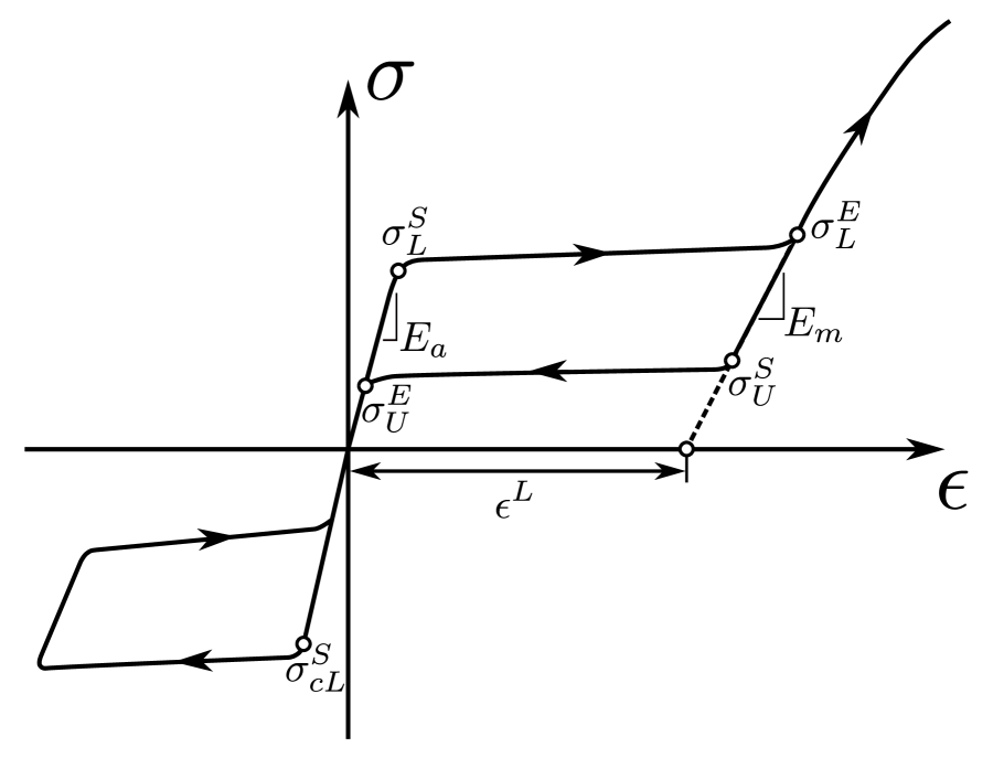
Figure 1: Notional uniaxial stress-strain curve for superelasticity UMAT in ABAQUS/Standard.

Table 1: Input parameters for superelastic UMAT in ABAQUS/Standard.

parameter	description
$E_{a}$	Young’s modulus, austenite
$\nu_{a}$	Poisson’s ratio, austenite
$E_{m}$	Young’s modulus, martensite
$\nu_{m}$	Poisson’s ratio, martensite
$\epsilon^{L}$	transformation strain
$\left(\frac{\partial\sigma}{\partial T}\right)_{L}$	change in transformation stresses with temperature, loading
$\sigma_{L}^{S}$	start of transformation, loading
$\sigma_{L}^{E}$	end of transformation, loading
$T_{0}$	reference temperature
$\left(\frac{\partial\sigma}{\partial T}\right)_{U}$	change in transformation stresses with temperature, unloading
$\sigma_{U}^{S}$	start of transformation, unloading
$\sigma_{U}^{E}$	end of transformation, unloading
$\sigma_{cL}^{S}$	start of transformation, compression
$\epsilon_{V}^{L}$	volumetric transformation strain

2.2 Simplifying assumptions

The superelastic constitutive model in ABAQUS uses pressure-dependent Drucker–Prager-like transformation surfaces and cubic transformation equations to define nonlinear hardening during phase transformation between austenite and martensite. As such, a general analytical solution to the associated rate equations is not easily obtained and to our knowledge has not been derived. Here, we instead derive an analytical solution for linear transformation behavior. Because of the way the nonlinear transformation equations are defined in ABAQUS, the linear and nonlinear transformation solutions should be equivalent at the beginning, mid-point, and end of both the loading (austenite $\rightarrow$ martensite) and unloading (martensite $\rightarrow$ austenite) transformations under the following assumptions (see Figure 2 and Table 2):

• symmetric transformation behavior in tension and compression, i.e. $\sigma_{L}^{S}=\sigma_{cL}^{S}$ (constitutive model becomes von Mises-like rather than Drucker–Prager-like)

• constant temperature (isothermal)

• equal elastic moduli for austenite and martensite, i.e. $E_{a}=E_{m}$

• pseudo-plasticity/superelasticity behavior only (i.e., the model is not superelastic-plastic)

• monotonic and proportional (i.e., radial) loading.

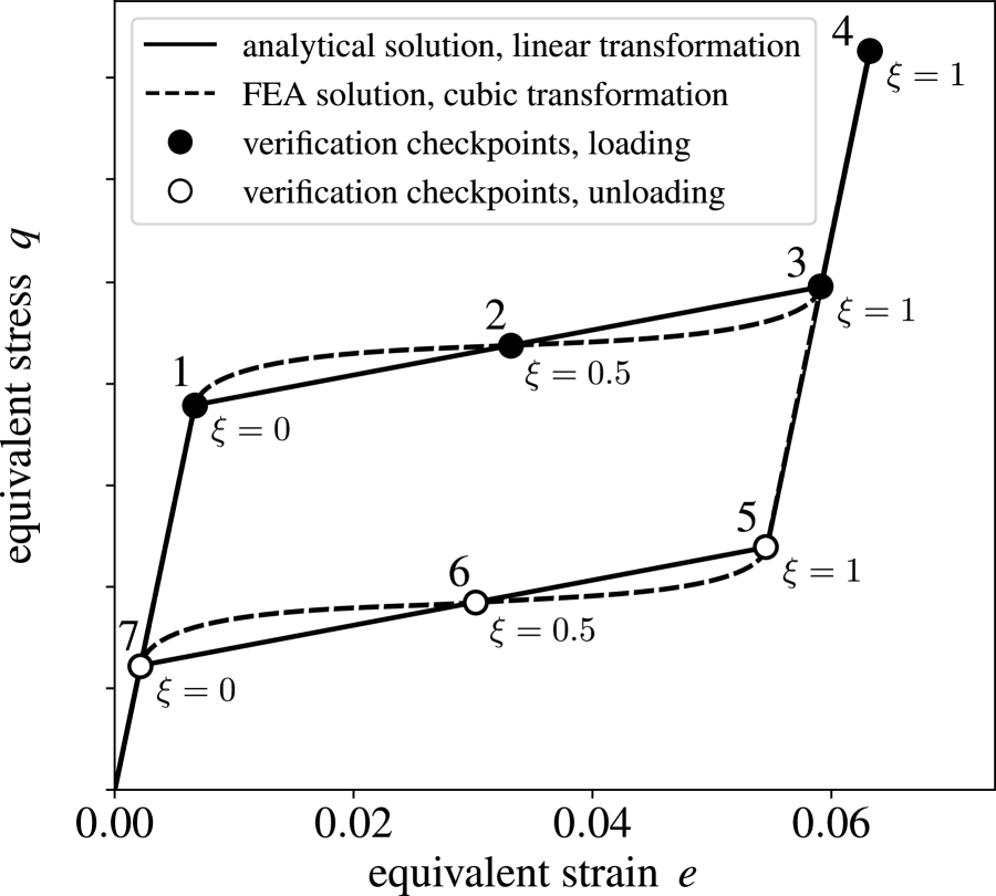
Figure 2: Illustration comparing the linear and nonlinear transformation solutions. Markers indicate locations at the beginning (1,5), mid-point (2,6), and end (3,7) of the loading and unloading transformation plateaus where the solutions are equivalent, and $\xi$ indicates the martensite fraction. The cubic shape of the nonlinear curve is exaggerated to facilitate visualization.

Table 2: Pairs of Mises equivalent stresses $q$ and martensite fractions $\xi$ defining verification points where the linear and nonlinear transformation solutions are equivalent. Note each combination of $q$ and $\xi$ defines a unique location in Figure 2.

		description	$q$	$\xi$
loading	1	beginning of transformation	$\sigma_{L}^{S}$	0.0
	2	mid-point of transformation	$\frac{\sigma_{L}^{S}+\sigma_{L}^{E}}{2}$	0.5
	3	end of transformation	$\sigma_{L}^{E}$	1.0
	4	end of loading (pure martensite)	$q_{\textrm{max}}$	1.0
unloading	5	beginning of transformation	$\sigma_{U}^{S}$	1.0
	6	mid-point of transformation	$\frac{\sigma_{U}^{S}+\sigma_{U}^{E}}{2}$	0.5
	7	end of transformation	$\sigma_{U}^{E}$	0.0

With these assumptions, we derive an exact analytical solution for the uniaxial strain of a single cubic element undergoing linear transformation and monotonic loading.

2.3 Problem description

Uniaxial strain of a unit cube is considered, i.e.,

$$\epsilon_{11} =f(t)$$ (1)

$$\epsilon_{22} =\epsilon_{33}=\epsilon_{12}=\epsilon_{13}=\epsilon_{23}=0$$ (2)

where $\epsilon_{ij}$ are the components of the logarithmic strain tensor and $t$ is the simulation pseudo-time for the elastostatic analysis. The cube has an initial side length $L_{0}=1$ and final side length in the direction of the applied strain of $L_{F}=L_{0}+u$, where $u$ is the applied displacement (Figure 3).

Figure 3: Schematic showing uniaxial strain of a unit cube with starting side length $L_{0}$ and final length $L_{F}=L_{0}+u$.

An unloading analysis is additionally performed to return the single element to the reference configuration.

During the loading and unloading analyses, the current length $l$ is defined as a linear ramping between $L_{0}$ and $L_{F}$,

$$l=\begin{cases}L_{0}+u\,t&\textrm{loading}\\ L_{0}+u\left(1-t\right)&\textrm{unloading}\end{cases}$$ (3)

with pseudo-time $t$ in the range

$$0<t<1\,.$$ (4)

We can also quantify the deformation using the non-dimensional stretch,

$$\lambda=\frac{l}{L_{0}}=\begin{cases}1+\frac{u\,t}{L_{0}}&\textrm{loading}\\ 1+\frac{u\left(1-t\right)}{L_{0}}&\textrm{unloading.}\end{cases}$$ (5)

2.4 Analytical solution

The exact analytical solution is derived in detail in the Appendix. In summary, given

• Mises stress $q$ and martensite fraction $\xi$ at the verification points in Table 2,

• shear and bulk moduli $G$ and $K$,

• assumptions from Section 2.2,

the analytical solutions for pseudo-time and the remaining field variables are summarized in Table 3.

Table 3: Analytical solutions for key quantities of interest at verification points $\left(q,\,\xi\right)$ listed in Table 2 and illustrated in Figure 2.

description	parameter	expression
total logarithmic strain	$\epsilon$	$\frac{q}{2G}+\frac{3}{2}\epsilon^{L}\xi$
hydrostatic pressure	$p$	$-K\epsilon$
deviatoric stress tensor	$\mathbf{S}$	$\frac{2}{3}q\,\mathbf{n}$
Cauchy stress tensor	$\boldsymbol{\sigma}$	$\mathbf{S}-p\mathbf{I}$
stretch	$\lambda$	$\exp\left(\epsilon\right)$
simulation pseudo-time	$t$	$\begin{cases}\frac{L_{0}(\lambda-1)}{u}&\text{loading}\\ 1-\frac{L_{0}(\lambda-1)}{u}&\text{unloading}\end{cases}$

2.5 Numerical simulations

Single-element verification simulations were performed in ABAQUS/Standard versions R2016x and 2022 using a single core of an Intel Xeon E5-4627 v4 processor. Commonly used continuum element types C3D8, C3D8R, C3D8I, C3D20, and C3D20R are investigated in both software versions. Material constants are prescribed as defined in Table 4. The input files for all cases are provided in supplemental material.

ABAQUS solves nonlinear mechanics problems in an incremental fashion for each simulation “step” or load sequence. For the present verification exercise, multiple steps are defined to facilitate extraction of field outputs at the precise pseudo-times where the analytical and numerical solutions agree if the constitutive code is correctly implemented (Tables 2 and 3). Displacement-controlled boundary conditions are prescribed to enforce the uniaxial strain conditions described in Eqn. 1–3. Increment sizes are defined such that each step consists of 100 increments. Numerical calculations of Mises stress $q$, uniaxial strain $\epsilon_{11}$, and stress components $\sigma_{11}$, $\sigma_{22}$, and $\sigma_{33}$ are extracted at each pseudo-time point using an ABAQUS/Python script. Note these results could also be obtained from ABAQUS printed output provided such output is requested at appropriate simulation pseudo-times. For elements with multiple integration points, quantities of interest are averaged across all integration points. Percentage error magnitudes between the numerical and analytical solutions are calculated as $|\phi_{\textrm{numerical}}-\phi_{\textrm{analytical}}|/\phi_{\textrm{analytical}}\times 100$ for each quantity of interest $\phi$.

A second set of single-element verification simulations using traction boundary conditions was also performed. In brief, the moving displacement boundary condition used above was replaced with a pressure boundary condition, with the prescribed pressure equal to the negative of the $\sigma_{11}$ component of the Cauchy stress tensor from the analytical solution (Table 3).

Table 4: Input variables for single-element verification problem.

description	parameter	value	units
initial length	$L_{0}$	1	mm
maximum displacement	$u$	0.1	mm
shear modulus	$G$	19,000	MPa
bulk modulus	$K$	42,000	MPa
Young’s modulus	$E_{\left\{a,m\right\}}$	$\frac{9KG}{3K+G}$	MPa
Poisson’s ratio	$\nu_{\left\{a,m\right\}}$	$\frac{3K-2G}{2(3K+G)}$	–
transformation strain	$\epsilon^{L}=\epsilon_{V}^{L}$*	0.05	–
change in transformation stress with temperature	$\left(\frac{\partial\sigma}{\partial T}\right)_{\{L,U\}}$	0	$\frac{\textrm{MPa}}{{{}^{\circ}}C}$
start of transformation, loading	$\sigma_{L}^{S}=\sigma_{cL}^{S}$	370	MPa
end of transformation, loading	$\sigma_{L}^{E}$	410	MPa
reference temperature	$T_{0}$	0	°C
start of transformation, unloading	$\sigma_{U}^{S}$	160	MPa
end of transformation, unloading	$\sigma_{U}^{E}$	120	MPa
*The input of a desired volumetric transformation strain $\epsilon_{V}^{L}$ in ABAQUS other than $\epsilon^{L}$ toggles
the use of a non-associated flow rule. Because the model herein simplifies to Mises-equivalent
transformation, the volumetric transformation strain is automatically zero.

3 Results

Each single-element simulation was completed within approximately 30 seconds with no clear influence of element type or solver version on simulation time (25.7 $\pm$ 1.3 sec and 35.6 $\pm$ 3.4 sec for displacement- and traction-controlled simulations, respectively). Simulations converged at each pseudo-time increment without the need for decreasing the increment size. Qualitatively, the numerical and analytical solutions are identical across all element types and software versions considered (Figure 4). The loading and unloading plateaus exhibit relatively large stiffnesses under uniaxial strain conditions compared to those associated with uniaxial stress conditions (Figure 4). Indeed, the $\sigma_{11}$ Cauchy stresses reach values nearly an order of magnitude larger under uniaxial strain conditions.

Quantitatively, for the displacement-controlled simulations, the results are relatively insensitive to the continuum element type or software version used, and extracted stress and strain measures are equivalent to within six to eight significant figures (see Supplemental Materials). One exception is the final equilibrium state after unloading where small residual stresses and strains are observed (Table 5). Comparing the analytical and numerical results, maximum errors in stress and strain are on the order of one ten-thousandth of a percent (Table 5). Although differences in the percent error magnitudes are observed among the various solver versions and element types investigated, the differences are relatively small. Accordingly, only the largest error magnitudes are reported in Table 5 for brevity.

Results are similar for traction-controlled conditions, although percent error magnitudes increase to approximately 1e-03 at the end of transformation in both loading and unloading. One exception is encountered using C3D8I elements, where percent error magnitudes reach approximately 1% at the end of transformation in unloading, and finite residual stresses and strains are observed at the end of unloading. For full details, see the supplemental material.

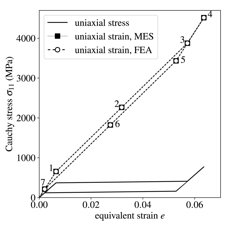
Figure 4: Comparison of the numerical and analytical results under uniaxial strain conditions. The corresponding superelastic stress-strain curve under uniaxial stress is also shown for reference.

Table 5: Numerical quantities of interest and percent error magnitudes calculated at the verification time points using displacement-controlled boundary conditions. The final row shows the largest deviations from the anticipated zero-stress and zero-strain condition across the simulations performed. The final three columns likewise report the maximum percent error magnitudes (% err.) observed across all simulations comparing the numerical and analytical solutions. Percent error magnitudes are omitted for the last row given division by zero. Stresses are in units of megapascals (MPa). For full results using each solver version and element type, see supplemental material.

step	$t$	$q$	$\epsilon_{11}$	$\sigma_{11}$	$\sigma_{\{22,33\}}$	$\epsilon_{11}$ % err.	$\sigma_{11}$ % err.	$\sigma_{\{22,33\}}$ % err.
1	0.09784	370	0.009737	655.6	285.6	3.806e-06	3.267e-06	3.187e-06
2	0.4892	390	0.04776	2266	1876	5.419e-07	6.237e-06	1.027e-06
3	0.8958	410	0.08579	3876	3466	2.121e-06	4.420e-07	4.942e-07
4	1	771.8	0.09531	4518	3746	6.165e-06	7.726e-06	3.672e-06
5	0.1757	160	0.07921	3434	3274	1.168e-06	4.990e-07	5.234e-07
6	0.5796	140	0.04118	1823	1683	3.009e-06	5.874e-06	6.362e-06
7	0.9684	120	0.003158	212.6	92.63	1.078e-04	1.088e-04	1.179e-04
8	1	3.796e-04	1.000e-08	6.739e-04	2.943e-04	N/A	N/A	N/A

4 Discussion and Conclusions

Using the method of exact solutions, we demonstrate verification of the superelastic constitutive model implemented in the ABAQUS/Standard implicit finite element solver. Specifically, uniaxial strain conditions are used to facilitate derivation of a closed-form solution for monotonic loading and unloading through the full range of transformation behavior. Although the uniaxial conditions are relatively simple to implement, they generate a nontrivial stress state that differs from the uniaxial stress condition typically used for model calibration. The verification exercise is performed by extracting quantities of interest at specific simulation increments where the numerical and analytical solutions should theoretically agree if the superelastic model is properly implemented. Simulation results reveal maximum errors in quantities of interest are on the order of one ten-thousandth of a percent, providing evidence that the model is indeed correctly implemented. The results are quantitatively similar for all solver versions and continuum element types investigated.

Note that, while we observe relatively small error magnitudes, the errors exceed machine precision for the double-precision floating-point operations performed by ABAQUS/Standard. A potential explanation is numerical incrementation. Each ABAQUS solution is computed in 800 increments, and there is a potential for errors to be generated at each increment. The results do not indicate obvious trends in error magnitude with increasing pseudo-time increment during loading. Accordingly, errors generated through incrementation are either negligible compared to the overall observed error magnitudes, or they are offset by subsequent increments such that they do not accumulate in simulation pseudo-time. In contrast, error magnitudes do increase i) during unloading when using C3D8I elements in the 2022 solver under displacement control, and ii) at the end of transformation for all element types and solver versions under traction control (see supplemental material), possibly due to incrementation error. The largest error magnitudes are observed at the end of unloading when using the C3D8I elements under traction control. Based on further investigation, this latter observation is uniquely associated with a combination of C3D8I elements, traction boundary conditions, and the superelastic model and is believed to be caused by the particular formulation of the incompatible mode element type.

A few limitations should be noted. First, although the fully integrated and simplified closed-form solution provided in Table 3 is convenient for performing the verification exercise, the solution is limited to strictly monotonic loading. Alternatively, the solution could be generalized to consider the activation and evolution of the martensite fraction $\xi$ under other loading paths, for example, unloading from the midpoint on the upper plateau (i.e., between verification points 2 and 6 in Figure 2). Second, a number of simplifying assumptions were used to derive the closed-form analytical solution. Consideration of tension-compression asymmetry, differences in austenite and martensite elastic moduli, and extensions of the superelasticity model such as the superelastic-plastic implementation could be investigated in future work. Third, the verification tests considered herein only address three-dimensional continuum elements using the implicit solver in ABAQUS. Verification using other element (e.g., beam and tetrahedral) and solver types (e.g., ABAQUS/Explicit) could be investigated in future work.

In conclusion, method of exact solutions code verification of the superelasticity model in ABAQUS was successful under uniaxial strain conditions. Code verification evidence like that generated by this study, alongside solution verification, experimental validation, and uncertainty quantification evidence, are useful to support the credibility of computational models, especially when model predictions are used to inform high-risk decision making. To facilitate reproducibility of this study using other hardware systems or software versions, and adaptation of the approach to other rate-based constitutive models, the full derivation of the analytical solution is provided in the Appendix, and simulation input files and post-processing scripts are provided as supplemental material.

Conflict of interest statement

One of the authors (NR) was formerly an employee of Dassault Systèmes Simulia, makers of ABAQUS.

Appendix A Appendix

In the following, standard typeface symbols are scalars (e.g., $\phi$), boldface symbols denote second-order tenors (e.g., $\mathbf{F}$ or $\boldsymbol{\sigma}$), and blackboard bold characters denote fourth-order tensors (e.g., $\mathbb{A}$). Additionally, the overdot operator (e.g., $\dot{A}$) indicates a time derivative.

A.1 General kinematic equations

Begin with the problem setup provided in Section 2.3 of the manuscript. The deformation gradient tensor is

$$\mathbf{F}=\mathbf{I}+\nabla\mathbf{u}$$ (6)

or, in matrix form,

$$\mathbf{F}=\begin{bmatrix}\lambda&0&0\\ 0&1&0\\ 0&0&1\end{bmatrix}$$ (7)

where $\mathbf{I}$ is the second-order identity tensor and $\lambda=\frac{l}{L_{0}}$ is the stretch. For finite-strain problems, ABAQUS solves the problem incrementally and calculates the strain by integrating the strain increments. The resulting strain measure is thus the logarithmic or “true” strain

$$\boldsymbol{\epsilon}=\ln\mathbf{V}$$ (8)

where $\ln$ is the principal matrix logarithm and

$$\mathbf{V}=\sqrt{{\mathbf{F}\mathbf{F}}^{T}}$$ (9)

is the left Cauchy stretch tensor.

Since $\mathbf{F}$ is diagonal here, $\mathbf{F}=\mathbf{F}^{T}$ and $\mathbf{V}=\mathbf{F}$. Therefore, the logarithmic strain tensor is simply $\ln\mathbf{F}$ or

$$\boldsymbol{\epsilon}=\begin{bmatrix}\ln\lambda&0&0\\ 0&0&0\\ 0&0&0\end{bmatrix}\,.$$ (10)

Since the only non-zero strain component for this uniaxial strain problem is $\epsilon_{11}$, let

$$\epsilon =\epsilon_{11}$$

$$=\ln\lambda$$ (11)

to simplify notation.

The volumetric strain $\epsilon_{V}$ is next defined as

$$\epsilon_{V} =\mathrm{tr}\,\boldsymbol{\epsilon}$$

$$=\epsilon_{11}+\epsilon_{22}+\epsilon_{33}$$

$$=\epsilon\,,$$ (12)

which represents a measure of volume change or dilation, where $\textrm{tr}\,\mathbf{A}=\mathbf{A}:\mathbf{I}$ is the trace operator for a second-order tensor and $\left(:\right)$ is the double-inner product operator $\mathbf{A}:\mathbf{B}=A_{ij}B_{ij}$. Note that the volumetric strain is sometimes defined in other literature as $\epsilon_{V}=\frac{1}{3}\textrm{tr}\,\boldsymbol{\epsilon}$, which represents a measure of mean normal strain.

The strain rate tensor

$$\dot{\boldsymbol{\epsilon}}=\begin{bmatrix}\dot{\epsilon}&0&0\\ 0&0&0\\ 0&0&0\end{bmatrix}$$ (13)

is obtained by taking the time derivative of $\boldsymbol{\epsilon}$. The deviatoric strain rate tensor $\dot{\mathbf{e}}$ is

$$\dot{\mathbf{e}}=\boldsymbol{\dot{\epsilon}}-\frac{1}{3}\,\textrm{tr}\,\dot{\boldsymbol{\epsilon}}\,\mathbf{I}\,,$$ (14)

or, in matrix form,

$$\dot{\mathbf{e}}=\begin{bmatrix}\frac{2}{3}\dot{\epsilon}&0&0\\ 0&-\frac{1}{3}\dot{\epsilon}&0\\ 0&0&-\frac{1}{3}\dot{\epsilon}\end{bmatrix}\,.$$ (15)

The scalar equivalent strain rate $\dot{e}$ is

$$\dot{e} =\sqrt{\frac{2}{3}\dot{\mathbf{e}}:\dot{\mathbf{e}}}$$

$$=\frac{2}{3}\dot{\epsilon}\,.$$ (16)

A.2 Equations for linear, monotonic transformation behavior

The superelastic constitutive model in ABAQUS [5, 6] is based on the work of Aurrichio and Taylor [7, 8] and leverages generalized plasticity theory to model the dependency of the material stiffness on the current stress state (see Online SIMULIA User Assistance 2022 >Abaqus >Materials >Elastic Mechanical Properties >Superelasticity). The constitutive model uses the additive strain rate decomposition

$$\dot{\boldsymbol{\epsilon}}^{e}=\dot{\boldsymbol{\epsilon}}-\dot{\boldsymbol{\epsilon}}^{\textrm{tr}}\,,$$ (17)

where $\dot{\boldsymbol{\epsilon}}^{e}$ is the elastic strain rate tensor and $\dot{\boldsymbol{\epsilon}}^{\textrm{tr}}$ is the transformation strain rate tensor. The Cauchy stress rate tensor is then

$$\dot{\boldsymbol{\sigma}}=\mathbb{D}:\dot{\boldsymbol{\epsilon}}^{e}$$ (18)

where $\mathbb{D}$ is the fourth-order elasticity or stiffness tensor and $\left(:\right)$ is the operator $\mathbb{A}:\mathbf{B}=A_{ijkl}B_{kl}$. For an isotropic material,

$$\mathbb{D}=2G\,\left(\mathbb{I}-\frac{1}{3}\,\mathbf{I}\otimes\mathbf{I}\right)+K\,\mathbf{I}\otimes\mathbf{I}\,,$$ (19)

where $G$ is the shear modulus, $K$ is the bulk modulus, $\left(\mathbf{I}\otimes\mathbf{I}\right)_{ijkl}=\delta_{ij}\delta_{kl}$, $\left(\mathbb{I}\right)_{ijkl}=\frac{1}{2}\left(\delta_{ik}\delta_{jl}+\delta_{il}\delta_{jk}\right)$, and $\delta_{ij}$ is the Kronecker delta function $\delta_{ij}=\begin{cases}0&i\neq j\\ 1&i=j\end{cases}$ [9]. Substituting Eqn. 19 into Eqn. 18 and simplifying, the Cauchy stress rate can be written in Hooke’s law form as

$$\dot{\boldsymbol{\sigma}} =2G\left(\dot{\boldsymbol{\epsilon}}^{e}-\frac{1}{3}\textrm{tr}\,\dot{\boldsymbol{\epsilon}}^{e}\mathbf{I}\right)+K\,\textrm{tr}\,\dot{\boldsymbol{\epsilon}}^{e}\mathbf{I}$$

$$=2G\dot{\mathbf{e}}^{e}+K\,\textrm{tr}\,\dot{\boldsymbol{\epsilon}}^{e}\mathbf{I}\,.$$ (20)

In ABAQUS, the flow rule describing the transformation strain rate for superelastic materials is

$$\dot{\boldsymbol{\epsilon}}^{\textrm{tr}}=\epsilon^{L}\,\dot{\xi}\,\frac{\partial G^{\textrm{tr}}}{\partial\boldsymbol{\sigma}}\,,$$ (21)

where $\epsilon^{L}$ is a material constant, $\xi$ is the martensite fraction, and $G^{\textrm{tr}}$ is a Drucker–Prager type transformation potential

$$G^{\textrm{tr}}=q-p\tan\psi\,.$$ (22)

In the above, $p$ is hydrostatic pressure, $\psi$ is a scaling constant, and $q$ is the von Mises stress

$$q=\sqrt{\frac{3}{2}\mathbf{S}:\mathbf{S}}\,,$$ (23)

where $\mathbf{S}$ is the deviatoric stress tensor

$$\mathbf{S}=\boldsymbol{\sigma}-\frac{1}{3}\,\textrm{tr}\boldsymbol{\sigma}.$$ (24)

As stated earlier, here we assume symmetric compression and tension behavior (i.e., $\sigma_{L}^{S}=\sigma_{cL}^{S}$). Thus, $\psi=0$, and the transformation potential takes on a von Mises form as simply

$$G^{\textrm{tr}}=q\,.$$ (25)

A.3 An aside: radial return and the direction tensor $\mathbf{n}$

Because the transformation behavior has been simplified as von Mises-type, the deviatoric stress and deviatoric strain rate tensors point in the same direction (in 6D space). The transformation potential is $q$, and the transformation strain rate is proportional to (i.e., in the direction of) the gradient of $q$ with respect to stress $\frac{\partial q}{\partial\boldsymbol{\sigma}}$, which we denote as $\mathbf{n}$. Expanding using Eqn. 23 and applying chain rule,

$$\mathbf{n} =\frac{\partial q}{\partial\boldsymbol{\sigma}}$$

$$=\frac{\partial\sqrt{\frac{3}{2}\mathbf{S}:\mathbf{S}}}{\partial\boldsymbol{\sigma}}$$

$$=\frac{\partial\left(\mathbf{S}:\mathbf{S}\right)^{\frac{1}{2}}}{\partial\mathbf{S}}\cdot\frac{\partial\mathbf{S}}{\partial\boldsymbol{\sigma}}$$

$$=\frac{1}{2}\left(\frac{3}{2}\mathbf{S}:\mathbf{S}\right)^{-\frac{1}{2}}\frac{3}{2}\left(2\mathbf{S}\right)\cdot\frac{\partial(\boldsymbol{\sigma}-\frac{1}{3}\,\textrm{tr}\boldsymbol{\sigma})}{\partial\boldsymbol{\sigma}}$$

$$=\frac{3}{2}\frac{\mathbf{S}}{q}\cdot(\mathbb{I}-\frac{1}{3}\,\mathbf{I}\otimes\mathbf{I})$$

$$=\frac{3}{2}\frac{\mathbf{S}}{q}\,.$$ (26)

Note the inner product of $\mathbf{n}$ with itself is

$$\mathbf{n}:\mathbf{n} =\frac{3}{2}\left(\frac{3}{2}\frac{\mathbf{S}:\mathbf{S}}{q^{2}}\right)$$ (27)

$$=\frac{3}{2}\frac{q^{2}}{q^{2}}$$

$$=\frac{3}{2}\,.$$

The double-inner product between the deviatoric stress tensor $\mathbf{S}$ and the direction of the deviatoric strain $\mathbf{n}$ is also useful since

$$\mathbf{S}:\mathbf{n} =\frac{3}{2}\frac{\mathbf{S}:\mathbf{S}}{q}$$

$$=\frac{q^{2}}{q}$$

$$=q\,.$$ (28)

Radial return algorithms project the trial stress back onto the yield (here transformation) surface by scaling the stress radially with respect to the hydrostatic axis $\sigma_{1}=\sigma_{2}=\sigma_{3}$, where $\sigma_{i}$ are principal stresses. We assume radial return to be exact under the given simplifications and approximations, specifically, equal transformation stresses in compression and tension and thereby von Mises-like transformation behavior, and proportional (radial) loading. Accordingly, the loading direction coincides with the projection direction and the (pseudo)plastic strain rate direction. As derived below,

$$\dot{\mathbf{e}}^{tr}=\dot{e}^{tr}\,\mathbf{n}$$ (29)

where $\dot{\mathbf{e}}^{tr}$and $\dot{e}^{tr}$ are the deviatoric transformation strain rate tensor and equivalent scalar, respectively, and $\mathbf{n}$ specifies the direction of the deviatoric transformation strain rate (the normal direction to the transformation surface with the given problem description). Following standard Mises plasticity arguments and given proportional loading, $\dot{\mathbf{e}}$ and $\dot{\mathbf{e}}^{tr}$are collinear. Accordingly, using Eqn. 16, the deviatoric strain rate tensor may also be written

$$\dot{\mathbf{e}} =\dot{e}\,\mathbf{n}$$

$$=\frac{2}{3}\dot{\epsilon}\,\mathbf{n}$$ (30)

and therefore, given Eqn. 15,

$$\mathbf{n}=\begin{bmatrix}1&0&0\\ 0&-\frac{1}{2}&0\\ 0&0&-\frac{1}{2}\end{bmatrix}\,.$$ (31)

A.4 Equations for linear, monotonic transformation behavior (continued)

Continuing from Eqn. 21, using Eqn. 25 and the definition of $\mathbf{n}$, the last term on the right-hand side becomes

$$\frac{\partial G^{\textrm{tr}}}{\partial\boldsymbol{\sigma}} =\frac{\partial q}{\partial\boldsymbol{\sigma}}$$

$$=\mathbf{n}\,.$$ (32)

The transformation strain rate from Eqn. 21 can thus be written

$$\dot{\boldsymbol{\epsilon}}^{\textrm{tr}}=\epsilon^{L}\,\dot{\xi}\,\mathbf{n}\,,$$ (33)

and the scalar equivalent transformation strain rate becomes

$$\dot{\epsilon}^{\textrm{tr}} =\sqrt{\frac{2}{3}\dot{\boldsymbol{\epsilon}}^{\textrm{tr}}:\dot{\boldsymbol{\epsilon}}^{\textrm{tr}}}$$

$$=\epsilon^{L}\,\dot{\xi}\,.$$ (34)

Note that $\mathbf{n}$ is deviatoric and $\textrm{tr}\,\mathbf{n}=0$. Therefore,

$$\textrm{tr}\,\dot{\boldsymbol{\epsilon}}^{\textrm{tr}}=0$$ (35)

and

$$\textrm{tr}\,\dot{\boldsymbol{\epsilon}}^{e} =\textrm{tr}\,\left(\dot{\boldsymbol{\epsilon}}-\dot{\boldsymbol{\epsilon}}^{\textrm{tr}}\right)$$

$$=\textrm{tr}\,\dot{\boldsymbol{\epsilon}}$$

$$=\dot{\epsilon}_{V}\,,$$ (36)

where $\dot{\epsilon}_{V}$ is the volumetric strain rate.

Using Eqns. 14, 17, and 33—36, the Cauchy stress rate from Eqn. 20 becomes

$$\dot{\boldsymbol{\sigma}} =2G\left[\left(\dot{\boldsymbol{\epsilon}}-\epsilon^{L}\,\dot{\xi}\,\mathbf{n}\right)-\frac{1}{3}\textrm{tr}\,\left(\dot{\boldsymbol{\epsilon}}-\epsilon^{L}\,\dot{\xi}\,\mathbf{n}\right)\mathbf{I}\right]+K\,\dot{\epsilon}_{V}\mathbf{I}$$

$$=2G\left[\left(\dot{\boldsymbol{\epsilon}}-\epsilon^{L}\,\dot{\xi}\,\mathbf{n}\right)-\frac{1}{3}\textrm{tr}\,\left(\dot{\boldsymbol{\epsilon}}\right)\mathbf{I}\right]+K\,\dot{\epsilon}_{V}\mathbf{I}$$

$$=2G\left(\dot{\mathbf{e}}-\epsilon^{L}\,\dot{\xi}\,\mathbf{n}\right)+K\,\dot{\epsilon}_{V}\,\mathbf{I}\,.$$ (37)

The Cauchy stress rate can be split into deviatoric and hydrostatic components

$$\dot{\boldsymbol{\sigma}}=\dot{\mathbf{S}}-\dot{p}\,\mathbf{I}\,,$$ (38)

where

$$\dot{\mathbf{S}}=2G\left(\dot{\mathbf{e}}-\epsilon^{L}\,\dot{\xi}\,\mathbf{n}\right)$$ (39)

is the deviatoric stress rate and

$$\dot{p}=-K\,\dot{\epsilon}_{V}$$ (40)

is the hydrostatic pressure rate.

The martensite fraction rate $\dot{\xi}$ is a function of the equivalent stress,

$$\dot{\xi}=f(q)\,,$$ (41)

and this function is called the transformation law (equivalent to a work-hardening law in plasticity). In general, the martensite fraction rate must be calculated for each increment, as its sign and magnitude depend on the current stress state as well as the direction and magnitude of the stress rate. However, for the linear hardening approximation and monotonic loading, we can define the martensite fraction directly as a linear function of the von Mises equivalent stress. For loading, we have

$$\xi_{\textrm{L}}\left(q\right)=\begin{cases}0&q\leq\sigma_{L}^{S}\\ \frac{q-\sigma_{L}^{S}}{\sigma_{L}^{E}-\sigma_{L}^{S}}&\sigma_{L}^{S}<q<\sigma_{L}^{E}\\ 1&q\geq\sigma_{L}^{E}\end{cases}\,,$$ (42)

and for unloading,

$$\xi_{\textrm{U}}\left(q\right)=\begin{cases}0&q\leq\sigma_{U}^{E}\\ \frac{q-\sigma_{U}^{E}}{\sigma_{U}^{S}-\sigma_{U}^{E}}&\sigma_{U}^{E}<q<\sigma_{U}^{S}\\ 1&q\geq\sigma_{U}^{S}\end{cases}\,.$$ (43)

For strictly monotonic proportional (constant $\mathbf{n}$) loading or unloading, we can now integrate the rate tensors in Eqns. 38—40 from $t=0$ to $t=t$ to obtain

$$\boldsymbol{\sigma}=\mathbf{S}-p\,\mathbf{I}$$ (44)

$$\mathbf{S}=2G\,\left(\mathbf{e}-\epsilon^{L}\,\xi\,\mathbf{n}\right)$$ (45)

$$p=-K\,\epsilon_{V}\,.$$ (46)

Similarly, substituting Eqn. 45 into Eqn. 28 and expanding using Eqns. 30 and 27, the equivalent stress $q$ becomes

$$q =\mathbf{S}:\mathbf{n}$$

$$=2G\left(\mathbf{e}:\mathbf{n}-\epsilon^{L}\,\xi\,\mathbf{n}:\mathbf{n}\right)$$

$$=2G\left(\frac{2}{3}\epsilon\,\mathbf{n}:\mathbf{n}-\epsilon^{L}\,\xi\,\mathbf{n}:\mathbf{n}\right)$$

$$=2G\left(\epsilon-\frac{3}{2}\epsilon^{L}\,\xi\right)$$

$$=2G\,\epsilon-3G\epsilon^{L}\,\xi\,.$$ (47)

Note the integrated equations take the same form for both loading and unloading. Pairings of $q$ and $\xi$, however, define specific locations on the stress-strain curve such that the solutions for loading and unloading are unique (see Figure 2 and Table 2).

A.5 Final analytical solution for uniaxial strain conditions

Given $q$ and $\xi$ (Table 2), solve Eqn. 47 for the total logarithmic strain $\epsilon$,

$$\boxed{\epsilon=\underbrace{\frac{q}{2G}}_{\text{elastic strain}}+\underbrace{\frac{3}{2}\epsilon^{L}\xi}_{\text{transformation strain}}}\,.$$ (48)

Next, use Eqn. 26 to calculate the deviatoric stress tensor,

$$\boxed{\mathbf{S}=\frac{2}{3}q\,\mathbf{n}}$$ (49)

and Eqns. 46 and 12 to calculate the hydrostatic pressure,

$$\boxed{p=-K\epsilon}\,.$$ (50)

Use Eqn. 44 to calculate the Cauchy stress tensor,

$$\boxed{\boldsymbol{\sigma}=\mathbf{S}-p\mathbf{I}}\,.$$ (51)

Finally, using Eqns. 5 and 11, calculate the corresponding solution pseudo-time $t$,

$$\boxed{t=\begin{cases}\frac{L_{0}\left(\lambda-1\right)}{u}&\text{loading}\\ 1-\frac{L_{0}\left(\lambda-1\right)}{u}&\text{unloading}\end{cases}}$$ (52)

where $\lambda=\exp\left(\epsilon\right)$.

References

- [1] ASME V&V40, “Assessing credibility of computational modeling through verification and validation: application to medical devices,” The American Society of Mechanical Engineers, 2018.
- [2] A. P. Baumann, T. Graf, J. H. Peck, A. E. Dmitriev, D. Coughlan, and J. C. Lotz, “Assessing the use of finite element analysis for mechanical performance evaluation of intervertebral body fusion devices,” JOR SPINE, vol. 4, no. 1, jan 2021.
- [3] K. I. Aycock, N. Rebelo, and B. A. Craven, “Method of manufactured solutions code verification of elastostatic solid mechanics problems in a commercial finite element solver,” Computers & Structures, vol. 229, p. 106175, 2020.
- [4] K. Kamojjala, R. Brannon, A. Sadeghirad, and J. Guilkey, “Verification tests in solid mechanics,” Engineering with Computers, vol. 31, no. 2, pp. 193–213, 2015.
- [5] N. Rebelo and M. Perry, “Finite element analysis for the design of nitinol medical devices,” Minimally Invasive Therapy & Allied Technologies, vol. 9, no. 2, pp. 75–80, 2000.
- [6] N. Rebelo, M. Hsu, and H. Foadian, “Simulation of superelastic alloys behavior with ABAQUS,” in SMST-2000: Proceedings of the International Conference on Shape Memory and Superelastic Technologies, 2001, pp. 457–469.
- [7] F. Auricchio and R. L. Taylor, “Shape-memory alloys: modelling and numerical simulations of the finite-strain superelastic behavior,” Computer Methods in Applied Mechanics and Engineering, vol. 143, no. 1-2, pp. 175–194, 1997.
- [8] F. Auricchio, R. L. Taylor, and J. Lubliner, “Shape-memory alloys: macromodelling and numerical simulations of the superelastic behavior,” Computer Methods in Applied Mechanics and Engineering, vol. 146, no. 3-4, pp. 281–312, 1997.
- [9] E. A. de Souza Neto, D. Peric, and D. R. Owen, Computational methods for plasticity: theory and applications. John Wiley & Sons, 2011.