Enhanced triplet superconductivity in next generation ultraclean UTe₂

Abstract

The spin-triplet superconductor UTe₂ exhibits a myriad of exotic physical phenomena, including the possession of three distinct superconducting phases at ambient pressure for magnetic field $\mu_{0}H\leq$ 40 T aligned in certain orientations. However, contradictory reports between studies performed on UTe₂ specimens of varying quality have severely impeded theoretical efforts to understand the microscopic properties of this material. Here, we report high magnetic field measurements on a new generation of ultraclean UTe₂ crystals grown by a salt flux technique, which possess enhanced superconducting critical temperatures and fields compared to previous sample generations. Remarkably, for $H$ applied close to the hard magnetic $b$ direction, we find that the angular extent of magnetic field-reinforced superconductivity is significantly increased in these pristine quality crystals. This suggests that in close proximity to a field-induced metamagnetic transition the enhanced role of magnetic fluctuations – that are strongly suppressed by disorder – is likely responsible for tuning UTe₂ between two distinct spin-triplet superconducting phases. Our results reveal a strong sensitivity to crystalline disorder of the field-reinforced superconducting state of UTe₂.

I Introduction

A superconducting state is attained when a material exhibits macroscopic quantum phase coherence. Conventional (BCS) superconductors possess a bosonic coherent quantum fluid composed of pairs of electrons that are weakly bound together by phononic mediation to form a Cooper pair [1, 2]. The condensation of Cooper pairs also drives superconductivity in unconventional superconductors, but in these materials the pairing glue originates not from phonons but instead from attractive interactions typically found on the border of density or magnetic instabilities [3]. The majority of known unconventional superconductors exhibit magnetically mediated superconductivity located in close proximity to an antiferromagnetically ordered state, comprising Cooper pairs in a spin-singlet configuration that have a total charge of 2$e$ and zero net spin [4, 5].

The discovery of superconductivity in the ferromagnetic metals UGe₂ [6], URhGe [7], and UCoGe [8] was surprising because most superconducting states are fragile to the presence of a magnetic field, as this tends to break apart the Cooper pairs that compose the charged superfluid. However, an alternative pairing mechanism was proposed for these materials, involving two electrons of the same spin combined in a triplet configuration, for which ferromagnetic correlations may thus enhance the attractive interaction [9].

The discovery of superconductivity below 1.6 K in UTe₂ [10] was also met with surprise, as although this material also exhibits several features characteristic of spin-triplet pairing, it possesses a paramagnetic rather than ferromagnetic groundstate. Two of the strongest observations in favor of triplet superconductivity in UTe₂ include a negligible change in the NMR Knight shift on cooling through the superconducting critical temperature ($T_{\text{c}}$), and large upper critical fields along each crystallographic axis that are considerably higher than the Pauli-limit for spin-singlet Cooper pairs [11]. Notably, for a magnetic field, $H$, applied along the hard magnetic $b$ direction, superconductivity persists to $\mu_{0}H\approx$ 35 T – over an order of magnitude higher than the Pauli limit [12, 13], at which point it is sharply truncated by a first-order metamagnetic (MM) transition into a field-polarised phase [14, 15]. Remarkably, this field-polarised state hosts a magnetic field-reentrant superconducting phase over a narrow angular range of applied field, which onsets at $\mu_{0}H\approx$ 40 T [14, 16, 17] and appears to persist to $\mu_{0}H\approx$ 70 T [18].

Careful angle-dependent resistivity measurements in high magnetic fields, for field applied in close proximity to the $b$-axis, observed that there appear to be two distinct superconducting phases over the field interval of 0 T $\leq\mu_{0}H\lessapprox$ 35 T [14, 15]. This interpretation has recently been corroborated by bulk thermodynamic measurements at this field orientation, indicating the presence of a distinct field-reinforced superconducting state for $\mu_{0}H\gtrapprox 15$ T [19]. Throughout this report we shall refer to the zero field superconducting state as SC1, to the field-reinforced phase for field applied close to the $b$ direction as SC2, and to the very high magnetic field-reentrant phase, located at $\mu_{0}H\gtrapprox$ 40 T for inclined angles in the $b-c$ rotation plane, as SC3.

Several early studies of the superconducting properties of UTe₂ observed two superconducting transitions in the temperature dependence of the specific heat (in zero applied magnetic field) [10, 20, 21], leading to speculation regarding a possible multi-component nature of the superconducting order parameter at ambient pressure and magnetic field. However, subsequent reports demonstrated that this was perhaps instead an artifact of sample inhomogeneity [22, 11], with higher quality samples found to exhibit a singular sharp superconducting transition [23, 24, 25]. Kerr effect measurements on samples exhibiting two specific heat transitions yielded evidence for time reversal symmetry breaking [20]; however, this observation could not be reproduced on higher quality samples [26]. Theoretical efforts to understand the microscopic details of the remarkable superconducting properties of UTe₂ have thus been stymied by these discrepancies between experimental studies performed on samples of varying quality.

In this work we report measurements on a new generation of UTe₂ crystals grown by a molten salt flux (MSF) method, using starting materials of elemental uranium refined by the solid state electrotransport technique [27] and tellurium pieces of 6N purity. The pristine quality of the resulting single crystals is evidenced by their high $T_{\text{c}}$ values of up to 2.10 K, low residual resistivities down to 0.48 $\upmu\Omega$ cm, and the observation of magnetic quantum oscillations at high magnetic fields and low temperatures [25]. Concomitant with the enhancement in $T_{\text{c}}$, the upper critical fields ($H_{\text{c2}}$) of SC1 along the $a$ and $c$ directions are also enhanced in comparison to samples with lower $T_{\text{c}}$ values. Notably, we also find that the angular extent of SC2 – that is, the rotation angle away from $b$ over which a zero resistance state is still observed at low temperatures for $\mu_{0}H\approx 30$ T – is significantly enhanced for this new generation of high purity crystals. We find that this can be well described by considering the enhanced role of magnetic fluctuations close to the MM transition.

By contrast, we find that the MM transition to the field polarised state still sharply truncates superconductivity at $\mu_{0}H_{m}\approx$ 35 T in MSF samples. This indicates that while the SC1 and SC2 superconducting phases of UTe₂ are highly sensitive to the effects of crystalline disorder, the first-order phase transition to the high magnetic field polarised paramagnetic state is an intrinsic magnetic feature of the UTe₂ system, and is robust against disorder. We also find that the formation of the SC3 phase in ultraclean MSF samples appears to follow the same field-angle profile found in prior sample generations grown by the chemical vapor transport (CVT) method.

II Experimental details

UTe₂ single crystals were grown by the MSF technique [28] using the methodology detailed in ref. [25]. Electrical transport measurements were performed using the standard four-probe technique, with current sourced along the $a$ direction. Electrical contacts on single crystal samples were formed by spot-welding gold wires of 25 $\upmu$m diameter onto the sample surface. Wires were then secured in place with a low temperature epoxy. All electrical transport measurements reported in this study up to maximal magnetic field strengths $\leq$ 14 T were performed in a Quantum Design Ltd. Physical Properties Measurement System (QD PPMS) at the University of Cambridge, down to a base temperature of 0.5 K. Electrical transport measurements up to applied magnetic field strengths of 41.5 T were obtained in a resistive magnet at the National High Magnetic Field Lab, Florida, USA, in a ³He cryostat with a base temperature of 0.35 K.

Skin depth measurements were performed using the proximity detector oscillator (PDO) technique [29]. This is achieved by measuring the resonant frequency, $f$, of an LC circuit connected to a coil of wire secured in close proximity to a sample, in order to achieve a high effective filling factor, $\eta$. As the magnetic field is swept, the resulting change in the resistivity, $\rho$, and magnetic susceptibility, $\chi_{s}$, of the sample induce a change in the inductance of the measurement coil. This in turn shifts the resonant frequency of the PDO circuit, which may be expressed as

$$\frac{\Delta f}{f}\approx-\eta\frac{\delta}{d}\left(\mu_{r}\frac{\Delta\rho}{\rho}+\Delta\chi_{s}\right),$$ (1)

where $d$ is the sample thickness, $\mu_{r}=\chi_{s}+1$, and the skin depth $\delta$ may be written as $\delta=\sqrt{\frac{2\rho}{\mu_{r}\mu_{0}\omega}}$, for excitation frequency $\omega$ [29, 30]. Thus, the PDO measurement technique is sensitive to changes in both the electrical resistivity and the magnetic susceptibility of the sample.

Steady (dc) field PDO measurements were performed at the National High Magnetic Field Lab, Florida, USA. One set of measurements was performed in an all-superconducting magnet utilising a dilution fridge sample space, over the temperature- and field-ranges of 20-100 mK and 0-28 T. Higher temperature, higher field measurements were obtained using a resistive magnet fitted with a ³He sample environment. Pulsed magnetic field PDO measurements were performed at Hochfeld-Magnetlabor Dresden, Germany, down to a base temperature of 0.6 K and up to a maximum applied field strength of 70 T.

III Enhancement of $T_{\text{c}}$ and $H_{\text{c2}}$ of SC1

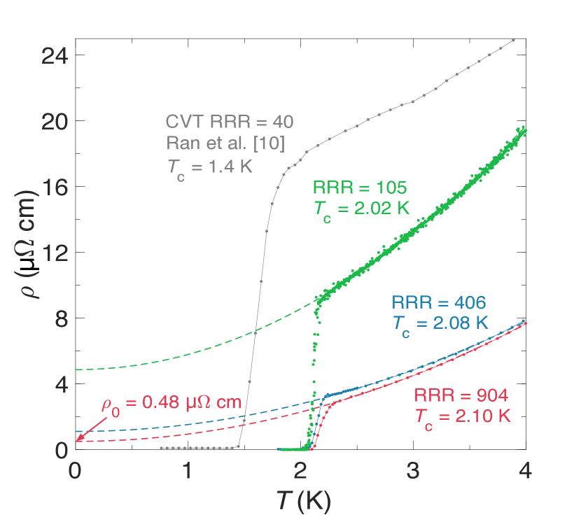
Figure 1: Electrical resistivity, $\rho$, as a function of temperature, $T$, for three samples grown by the molten salt flux (MSF) technique (colored points), plotted alongside data reported for a chemical vapor transport (CVT) specimen in ref. [10]. $T_{\text{c}}$ values were determined by zero resistivity. Residual resistivity ratios (RRRs) were computed by fitting the low temperature normal state resistivity with the dashed curves, of functional form $\rho=AT^{2}+\rho_{0}$ for constant $A$, to extract the residual normal state resistivity $\rho_{0}$. The dimensionless RRR value is defined as $\rho(T=$ 300 K$)/\rho_{0}$.

Table 1: Comparison of critical superconducting temperature ($T_{\text{c}}$), residual resistivity ($\rho_{0}$), and the residual resistivity ratio (RRR) for UTe₂ samples grown by the MSF and CVT techniques from various reports as indicated. In all cases, $T_{\text{c}}$ is defined by zero resistivity, which we identify as the first measurement point to fall below 0.1 $\upmu\Omega$ cm on cooling. $\rho_{0}$ is determined by a quadratic fitting at low temperatures, as depicted in Figure 1, to give the expected normal state resistivity value at 0 K in the absence of superconductivity. RRR is the ratio between $\rho_{0}$ and $\rho$($T=$ 300 K). FIB stands for focused ion beam. Note that in Sakai et al. [28] the authors stated that their RRR = 1000 sample was too small to accurately determine the resistivity – therefore a value for $\rho_{0}$ was not obtained.

Growth method	$T_{\text{c}}$ (K)	$\rho_{0}$ ($\upmu\Omega~{}\mathrm{cm}$)	RRR	Reference
	2.10	0.48	904
MSF	2.08	1.1	406	This study
	2.02	4.7	105
MSF	2.06	1.7	220	Aoki et al. (2022) [24]
MSF	2.10	-	1000	Sakai et al.
	2.04	2.4	170	(2022) [28]
	2.00	7	88
CVT	1.95	9	70	Rosa et al. (2022) [23]
	1.85	12	55
CVT	1.44	16	40	Ran et al. (2019) [10]
CVT	1.55 - 1.60	19	35	Aoki et al. (2019) [31]
CVT	1.55 - 1.60	16	35 - 40	Helm et al.
CVT FIB	1.55 - 1.60	27	25 - 30	(2022) [18]

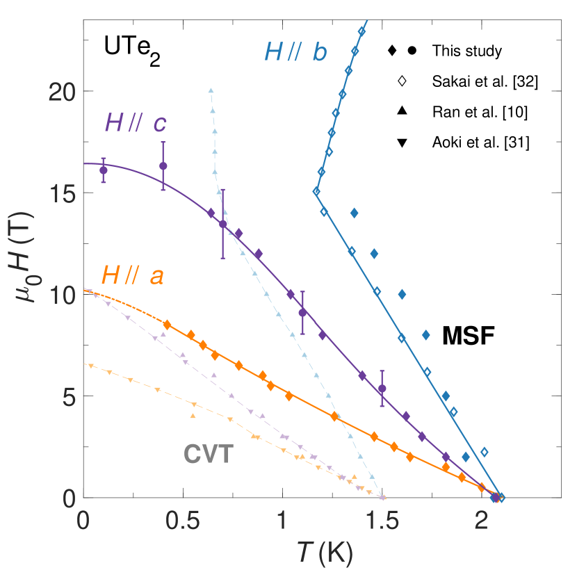
Figure 2: Magnetic field–temperature superconducting phase diagram of UTe₂. For field oriented along each crystallographic axis, $T_{\text{c}}$($H$) is enhanced for MSF samples (bold symbols) in comparison to CVT samples (pale symbols). Lines are given as a guide to the eye. Contacted (contactless) resistivity measurements from this study are represented by solid diamonds (circles). Raw resistivity data used in part to construct this figure are given in Appendix B. The procedure for determining error bars for contactless resistivity points is detailed in Appendix A. All contacted resistivity measurements were performed on the RRR = 406 sample from Table 1. Additional MSF resistivity data along the $b$ direction are reproduced from ref. [32]. CVT resistivity data are given by up (down) triangles, reproduced from ref. [10] (ref. [31]). We identify the normal-superconducting transition temperature by the point at which zero resistivity is first attained, as defined in Table 1.

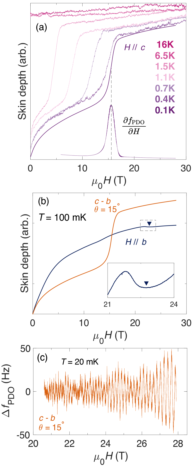
Figure 3: (a) PDO measurement of the skin depth of UTe₂ for magnetic field applied along the $c$ direction at various temperatures (strictly, this is a measurement of $\frac{\Delta f}{f}$ as per Eq. 1, which we refer to as skin depth for succinctness). The derivative of the 0.1 K curve is also plotted ($\frac{\partial f_{\text{PDO}}}{\partial H}$), identifying the superconducting transition out of the SC1 state. These data form part of Fig 1. (b) Skin depth for field oriented along the $b$ direction (dark blue curve) and tilted 15$\degree$ from $c$ towards $b$ (ochre curve). The inset shows a zoomed view of the $H\parallel b$ data, with an arrow marking the location of an anomalous feature that appears to indicate the boundary between SC1 and SC2. (c) Oscillatory component of the PDO signal at 20 mK, showing prominent quantum oscillations of frequencies $\approx$ 3.5 kT, consistent with prior studies [24, 25]. All data in this figure were collected on the same sample.

Figure 1 shows the temperature dependence of the electrical resistivity, $\rho(T)$, for three MSF samples (colored points) of varying quality. Data for $\rho(T)$ of a CVT sample reported in ref. [10] is plotted in gray for comparison. A clear trend is apparent, with samples exhibiting higher $T_{\text{c}}$ values also possessing higher residual resistivity ratios (RRRs), where the RRR is the ratio between the residual resistivity, $\rho_{0}$, and $\rho$($T=$ 300 K).

Table 1 tabulates these data presented in Fig. 1, and also includes data from other studies as indicated. Here, the correlation between $T_{\text{c}}$ and RRR is further emphasised, with samples exhibiting high $T_{\text{c}}$ values also possessing low residual resistivities (and thus high RRRs). A high RRR is indicative of high sample purity [23], as samples containing less crystalline disorder will thus have lower scattering rates for the charge carriers partaking in the electrical transport measurement. Characterising sample quality by comparison of RRR values is a particularly effective methodology, as it is agnostic with regards to the source of the crystalline disorder – be it from grain boundaries or vacancies or impurities, from some other source of disorder, or indeed a combination of several types. The presence of any such defects will lead to an increase in the charge carrier scattering rate, thereby yielding a lower resultant RRR.

Figure 2 shows a comparison of the extent of superconductivity for CVT and MSF samples. For magnetic field applied along the crystallographic $a$ and $c$ directions, $H_{c2}$ is clearly enhanced for the cleaner MSF samples, in good agreement with ref. [33]. Along the hard magnetic $b$ direction, $T_{\text{c}}$($H$) is also enhanced for all temperatures measured. The effect of magnetic field-reinforced superconductivity along this direction is observed as a kink in the $T_{\text{c}}$($H$) curve at $\mu_{0}H\approx$ 15 T, as reported previously [14, 19] – but this feature occurs at higher temperature in the case of MSF-grown UTe₂ compared to CVT samples. We also find that the lower critical field ($H_{c1}$) is enhanced for MSF samples, consistent with a recent report [34], as shown in Appendix B.

This observation of increased sample purity leading to an enhancement of $T_{\text{c}}$ and $H_{c}$ is not uncommon for unconventional superconductors, with a strong correlation between $T_{\text{c}}$ and $\rho_{0}$ previously reported, for example, in studies of ruthenates [35], cuprates [36], and heavy fermion superconductors [37, 38]. A quantitative analysis of the effect of crystalline disorder can often be achieved by utilizing the Abrikosov-Gor’kov theory [39]. However, it has been suggested that this approach does not appear to be valid for the case of UTe₂ [40], indicating a complex dependence of superconductivity on the presence of disorder, as may be expected for a $p$-wave superconductor.

The high purity of UTe₂ samples investigated in this study is further underlined by their ability to exhibit the de Haas-van Alphen (dHvA) and Shubnikov-de Haas (SdH) effects at high magnetic fields and low temperatures. All measurements reported in this study were performed on crystals from the same batch as those previously reported [25] to exhibit high frequency quantum oscillations, indicative of a long mean free path and thus high crystalline quality.

Figure 3 shows the PDO response of UTe₂ at low temperatures up to intermediate magnetic field strengths. Note that the response of the PDO circuit is expressed in full in Eq. 1 – for brevity, we shall refer to this throughout as the skin depth, as aspects of both $\rho$ and $\chi_{s}$ are important. Fig. 3(a) maps the superconducting phase boundary for $H\parallel c$. In Fig. 3(c) the oscillatory component ($\Delta f_{\text{PDO}}$) of the PDO signal at $T=$ 20 mK is isolated, which exhibits clear quantum oscillations. The observation of quantum oscillations in a material requires $\omega_{c}\tau\gtrsim$ 1, where $\omega_{c}$ is the cyclotron frequency and $\tau$ is the quasiparticle lifetime [41]. Therefore, the manifestation of quantum oscillations in our samples indicates that the mapping of the UTe₂ phase diagram presented in this study gives an accurate description of the UTe₂ system in the clean quantum limit.

IV Pronounced angular enhancement of SC2

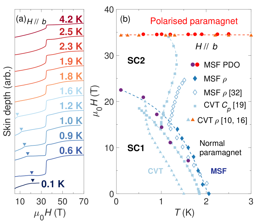
Figure 4: (a) PDO measurements for $H\parallel b$ at indicated temperatures. The 0.1 K curve is the same data as in Fig. 3b, measured in a dc magnet; all other data were obtained in a pulsed magnet. Arrows indicate the anomalous feature in the PDO signal displayed in Fig.  3b, marked by purple circles in panel (b), which indicates a magnetic field-induced transition between two superconducting states (SC1 and SC2). (b) Field-temperature phase diagram comparing the phase-space of CVT and MSF UTe₂ samples for $H\parallel b$. Points are from refs [10, 32, 16, 19] as indicated. Lines are as a guide to the eye. Two distinct superconducting phases are observed at low temperatures for this field orientation, which we label as SC1 and SC2. The extent of both SC1 and SC2 in temperature is clearly enhanced for MSF samples compared to CVT specimens. However, both types of samples see the SC2 phase sharply truncated by a MM transition to a field polarised state at $\mu_{0}H_{m}\approx$ 35 T.

One of the most remarkable features of the UTe₂ phase diagram (at ambient pressure) is the presence of three distinct superconducting phases for magnetic field aligned along certain orientations [14]. For $H$ applied along the $b$ direction, at low temperatures ($T<$ 0.5 K) zero resistance is observed all the way up to 34.5 T [16]. Remarkably, at higher temperatures ($T\approx$ 1 K) and for field applied at a slight tilt angle away from $H\parallel b$, measurements of CVT samples have shown that rather than a single superconducting state persisting for 0 T $\leq\mu_{0}H\leq$ 34.5 T, there are instead two distinct superconducting phases present over this field interval [19], with the higher-field phase (SC2) having been referred to as a “field-reinforced” superconducting state [11].

Figure 4 shows the skin depth of UTe₂ measured in pulsed magnetic fields up to 70 T, for field applied along the hard magnetic $b$ direction. The MM transition to the polarised paramagnetic state is clearly observed by a sharp step in the skin depth at $\mu_{0}H_{m}\approx 35$ T for all temperatures [11]. An interesting aspect of our PDO measurements is the presence of an anomalous kink feature, marked with arrows in Fig. 4(a) (and in the inset of Fig. 3(b)), which appears to demarcate the phase boundary between SC1 and either SC2 or the normal state, depending on the temperature. These points are plotted as purple circles in Fig. 4, along with resistivity and specific heat data from previous reports [10, 32, 19, 16]. By Eq. 1 the change in frequency of the PDO circuit is sensitive to both the electrical resistivity and the magnetic susceptibility of the sample. Thus, this observation appears consistent with recent reports [32, 17] in which a kink in the magnetic susceptibility has been attributed to marking the termination of SC1, which is visible in our skin depth measurements even though the resistivity remains zero as the material passes from SC1 to SC2.

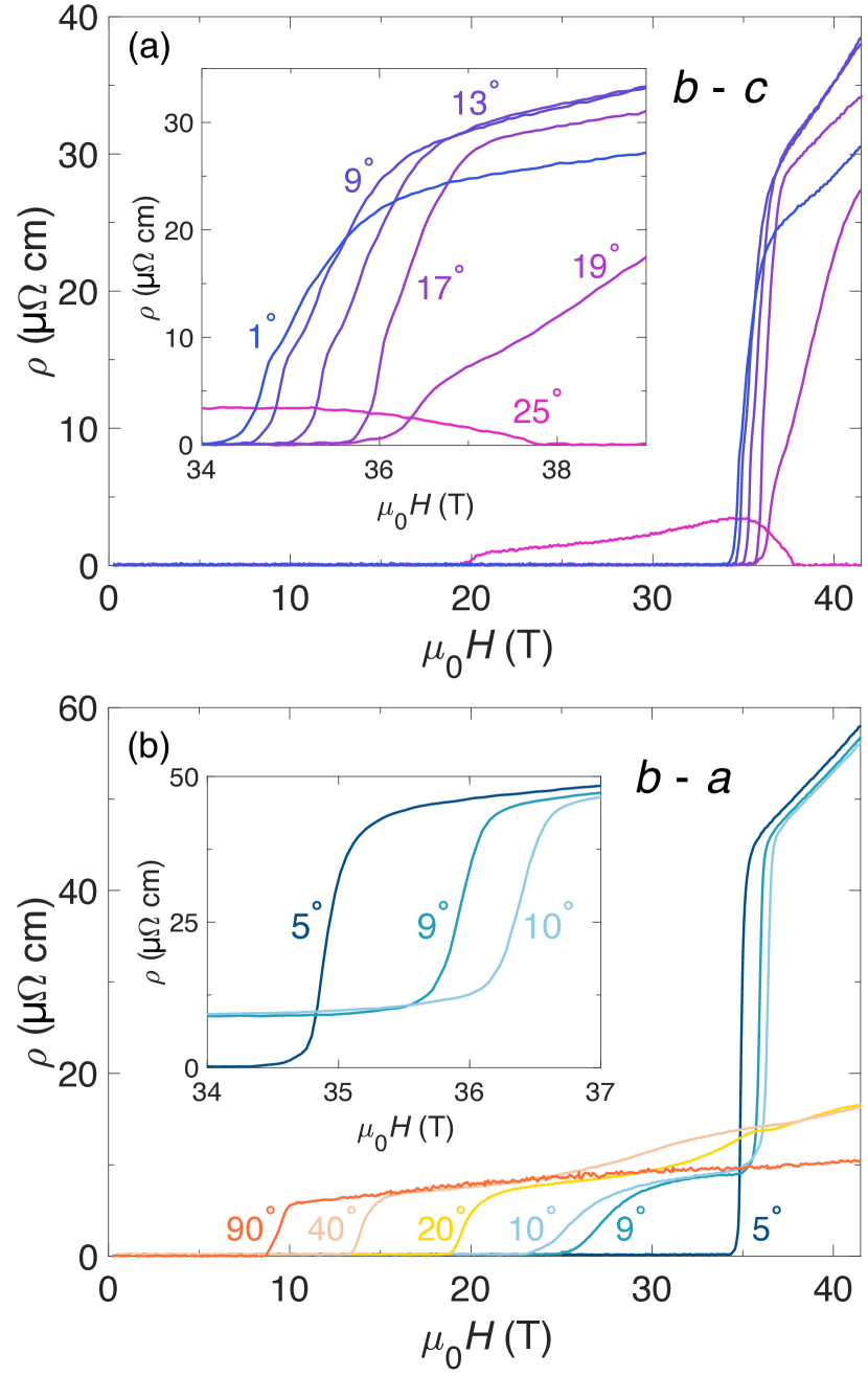
Figure 5: Angular dependence of resistivity for rotation in (a) the $b-c$ plane and (b) the $b-a$ plane. 0$\degree$ corresponds to $H\parallel b$ for both panels. Insets give a zoomed view of the magnetic field interval over which the MM transition is located. The data in panel (a) were recorded on the RRR = 406 sample from Table 1 while those in panel (b) are from the RRR = 105 sample. All data were obtained at $T=0.4$ K.

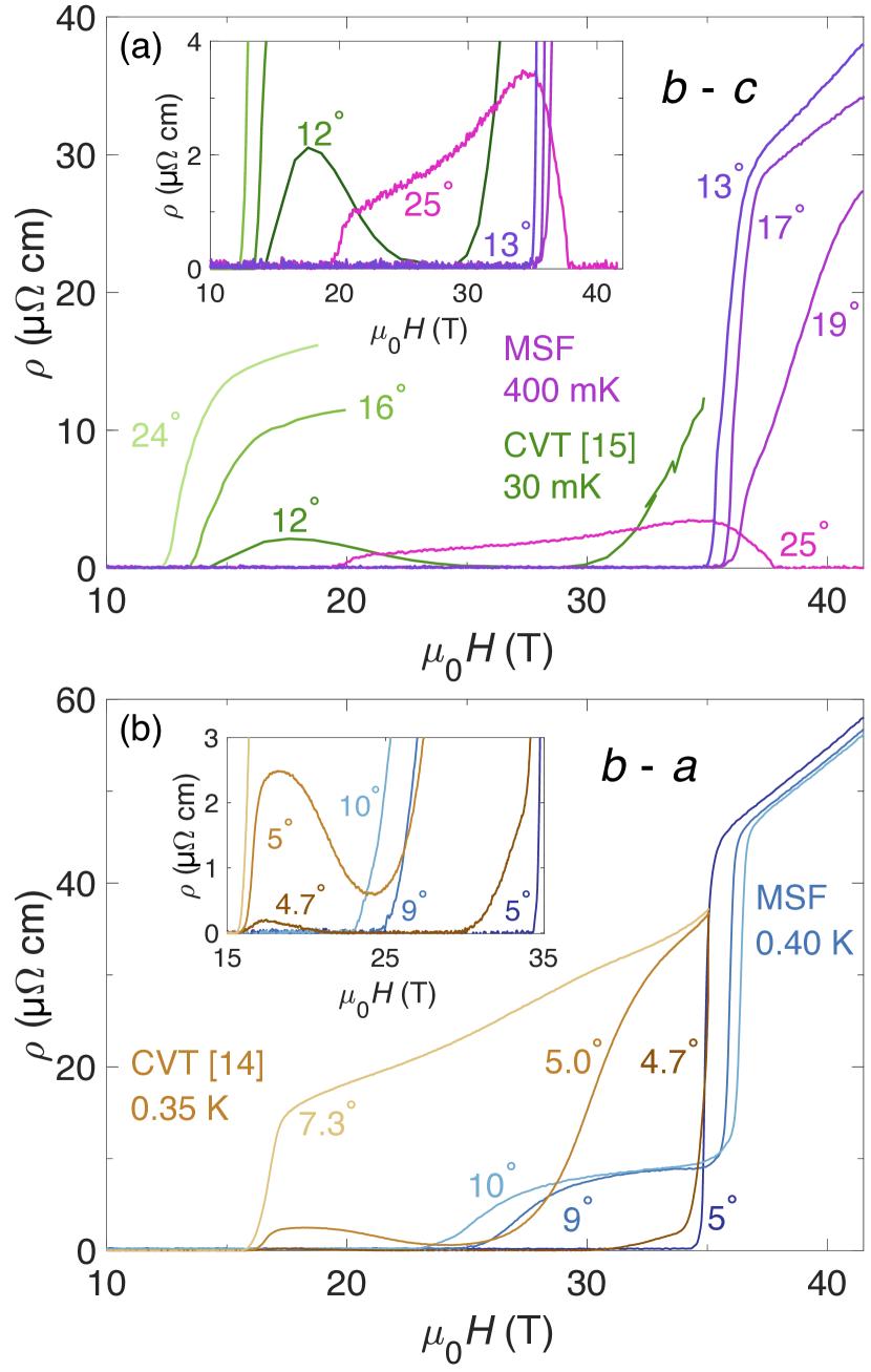
Figure 6: Comparison of UTe₂ $\rho(H)$ data for MSF and CVT samples in (a) the $b-c$ rotation plane and (b) the $b-a$ rotation plane. Insets give a zoomed view of the main panels. MSF curves for selected angles are reproduced from Fig. 5. CVT data in (a) are reproduced from ref. [15] while those in (b) are from ref. [14].

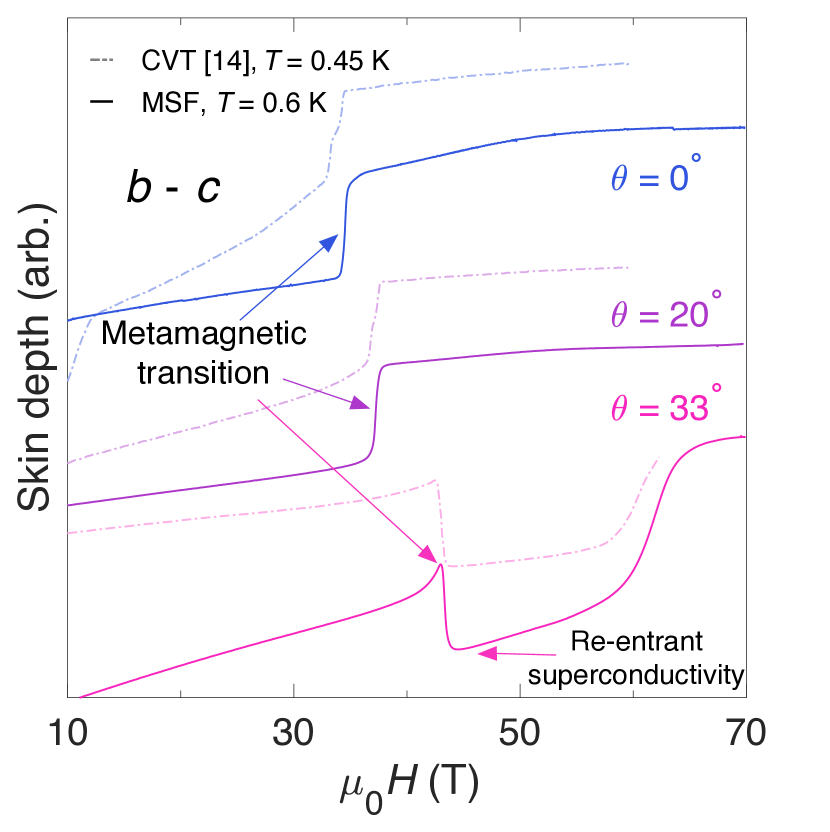
Figure 7: Angular evolution of the MM transition at high fields in the $b-c$ plane; $\theta=$ 0$\degree$ corresponds to $H\parallel b$. Notably, we find that the location of the MM transition is unchanged comparing between MSF (solid curves) and CVT (dashed curves from ref. [14]) samples, including for the onset of re-entrant superconductivity (SC3) at $\theta=~{}$33$\degree$.

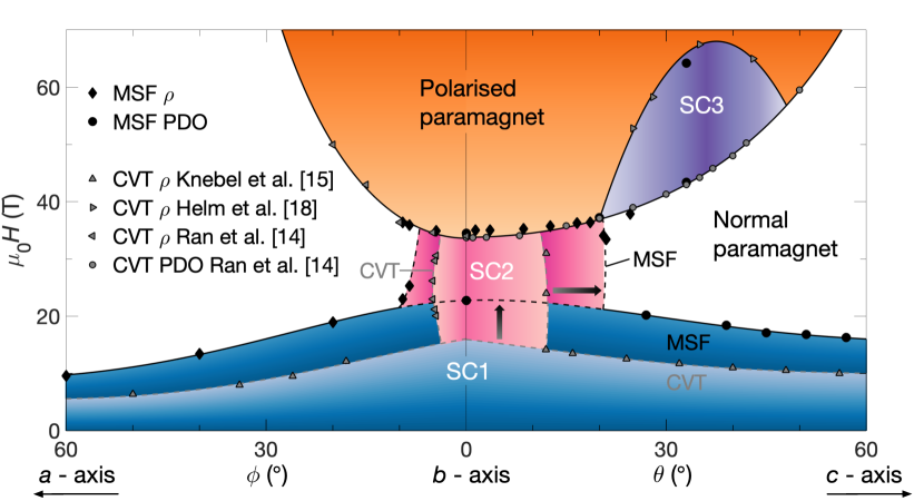
Figure 8: Angular magnetic field phase diagram of UTe₂ for $\mu_{0}H\leq 70$ T. The phase boundary between SC1 and the normal state is located at higher magnetic field strengths for MSF samples compared to prior studies on CVT specimens (blue region). Furthermore, the angular extent of SC2 is greatly enhanced for MSF samples (pink region). The polarised paramagnetic state (orange region) is found to have the same angular profile for both types of samples. Lines and shading are as a guide to the eye. CVT data points from refs. [15, 18, 14].

Figure 5 shows the resistivity of MSF-grown UTe₂ measured in a resistive magnet over the field interval 0 T $\leq\mu_{0}H\leq$ 41.5 T at $T=0.4$ K for various magnetic field tilt angles as indicated. Data in the $b-c$ plane were taken on the RRR = 406 sample from Table 1 while those in the $b-a$ plane are from the RRR = 105 sample.

At $T=0.4$ K, for small tilt angles within 5$\degree$ from the $b$ direction in both rotation planes, zero resistivity persists until the magnetic field strength exceeds 34.0 T, whereupon the resistivity increases rapidly at the MM transition as SC2 terminates and the polarised paramagnetic state is entered. In the $b-c$ rotation plane, this remains the case for angles up to 19$\degree$ away from $b$; however, by 25$\degree$ nonzero resistivity is observed at $\mu_{0}H$ as low as 20 T (Fig. 5(a)). Above 20 T the resistivity at this angle then remains small but nonzero up to 38 T. At this point the SC3 phase is accessed and zero resistivity is observed up to this measurement’s highest applied field strength of 41.5 T.

Figure 6 compares the angular extent of SC2 by collating selected angles from Fig. 5 alongside prior CVT studies. In the $b-c$ rotation plane, CVT measurements reported by Knebel et al. [15] found that for a rotation angle of 8$\degree$ away from $b$, zero resistivity persisted up to their highest accessed field strength of 35 T. However, at 12$\degree$ this was no longer the case, with nonzero resistance observed over the field interval of 14 T $\lessapprox\mu_{0}H\lessapprox$ 25 T. The resistivity then returned to zero for 25 T $\lessapprox\mu_{0}H\approx$ 30 T, above which it increased up until 35 T (Fig. 6(a)).

By contrast, our measurements on MSF-grown UTe₂ yield zero resistivity over the entire field interval 0 T $\leq\mu_{0}H\lessapprox$ 34.5 T for successive tilt angles up to and including 19$\degree$ away from $b$ towards $c$. Notably, our measurements in the $b-c$ plane were performed in a ³He system, at a temperature an order of magnitude higher than those reported by Knebel et al. [15]. This indicates a remarkable angular expansion of SC2 resulting from the enhancement of purity in this new generation of crystals.

A similar trend is found in the $b-a$ rotation plane. Prior measurements on a CVT specimen reported by Ran et al. [14] found a strong sensitivity of the extent of SC2 within a very small angular range of only 0.3$\degree$, with markedly different $\rho(H)$ observed for 4.7$\degree$ compared to 5.0$\degree$ (Fig. 6(b)). By comparison, at 5$\degree$ we observed zero resistance persisting to $\mu_{0}H>$ 34 T, while at 9$\degree$ and 10$\degree$ the resistive transition is notably sensitive to such a small change in angle, indicating that the boundary of SC2 for MSF samples lies close to here. Interestingly, it appears that the angular extent of SC2 in both rotation planes appears to be approximately doubled for MSF compared to CVT samples – for angles $b-c$ from approximately 12$\degree$ to between 19$\degree$-25$\degree$, and for $b-a$ from 5$\degree$ to around 10$\degree$.

V Field-angle phase space of UT$\text{e}_{2}$

The previous sections have demonstrated that the critical fields of SC1, and the angular extent of SC2, have been enhanced for this new generation of pristine quality UTe₂ crystals. We turn our attention now to consider the behavior of the field polarised state, which is instructive as it is this phase into which SC2 is abruptly quenched, and out of which SC3 emerges.

Fig. 4 shows a clear step in the skin depth for $H\parallel b$ at $\mu_{0}H\approx 35$ T. Extensive prior high magnetic field measurements on CVT-grown samples have identified this feature as a first-order MM transition to a polarised paramagnetic state at which the magnetization of the material abruptly jumps by $\approx$ 0.5 $\mu_{\text{B}}$ per formula unit [42, 11, 43, 14].

Figure 7 tracks the MM transition as the orientation of the magnetic field is rotated away from $b$ towards $c$, and compares with prior PDO measurements on a CVT specimen reported in ref. [14]. At $\theta=\{0\degree,20\degree\}$ the sharp rise in the skin depth – caused by the abrupt increase in resistivity characteristic of entering the polarised paramagnetic phase – occurs at the same value of $H$ for both CVT and MSF samples (within experimental resolution). At $\theta=33\degree$, again both samples see a jump in the skin depth at the same field strength – but here the jump is in the opposite direction, due to the presence of SC3.

Figure 8 depicts the phase space of UTe₂ for applied magnetic fields oriented in the $b-c$ and $b-a$ planes, at strengths up to 70 T, combining our MSF data with prior CVT studies. CVT $\rho$ from Knebel et al. [15] was reportedly measured at $T=$ 30 mK; our MSF PDO points tracking the termination of SC1 were measured at $T=0.1$ K. All our $\rho$ points in this figure were measured at $T=$ 0.4 K in steady fields, while the $\rho$ and PDO measurements reported by Ran et al. [14] were performed both in steady and pulsed fields, at $T\approx$ 0.4-0.5 K. Our pulsed field PDO measurements tracking the field polarised state, and the $\rho$ measurements reported in Helm et al. [18], were performed at $T\approx$ 0.6-0.7 K.

Upon inspecting Figs. 7 and 8, there appears to be negligible difference between measurements of the MM transition for MSF and CVT samples. This indicates that this transition is an intrinsic property of the UTe₂ system that, unlike SC1 and SC2, is insensitive to crystalline disorder. Furthermore, we find that the temperature evolution of the MM transition tracks very similarly between MSF and CVT samples, implying that the associated energy scale is unchanged under the improvement of sample quality (see Figure 16 in Appendix B for steady field data up to $T=$ 34 K) [44, 16].

VI Modelling the origin of SC2

The mechanism behind, and the precise form of, the superconducting order parameter in UTe₂ remains the subject of much theoretical debate [45, 46, 47, 48, 49, 50, 51, 52]. The current consensus appears to be that at zero external field a triplet order parameter is stabilized by some form of magnetic fluctuations, giving rise to the SC1 phase [11]. The experimental data suggests, however, that the SC2 phase has a rather different character, as evidenced by its acute sensitivity to the field direction, its starkly different NMR spectra, and by the observation of $T_{c}$ growing with increasing field aligned along the $b$-axis [52, 53, 32, 19].

These observations suggest that the SC2 phase likely has a very different pairing mechanism compared to SC1, with a distinct possibility being that it is driven by MM fluctuations. Such a mechanism for magnetic field-reinforced superconductivity has previously been considered in the case of the ferromagnetic superconductors URhGe and UCoGe [9, 54, 55, 56]. We theoretically model this scenario (taking $k_{\text{B}}=\hslash=1$ throughout) for the case of UTe₂ by first considering a Ginzburg-Landau theory describing the MM phase transition [57, 56, 58]:

$$\mathcal{F}[\mathbf{M}](\mathbf{H}) =\frac{1}{2}\chi^{-1}_{i}M_{i}^{2}+\frac{1}{4}\beta_{ij}M_{i}^{2}M_{j}^{2}+\frac{1}{6}\gamma M_{y}^{6}-\mathbf{M\cdot H}+$$

$$+\kappa_{j}(\partial_{j}M_{j})^{2}$$ (2)

where $i,j=x,y,z$, $\mathbf{M}$ is the magnetic order parameter, and $\chi^{-1}_{i},\beta_{ij},\gamma,$ and $\kappa_{j}$ are Ginzburg-Landau parameters. Good agreement with the experimental data is obtained only if $\beta_{xy}$ is non-zero (see caption of Fig. 9 for parameter values). We chose the parameters such that at zero applied field, the free energy has two minima: a global minimum at $\mathbf{M}=0$, and a minimum with higher energy at $\mathbf{M}=\mathbf{M}_{*}$ pointing along the $b$ direction. As the field is applied, the minimum at $\mathbf{M}_{*}$ decreases until it becomes the new global minimum at the metamagnetic phase transition point $H_{m}$. We denote the energy at this minimum as $\Omega_{*}(\mathbf{q})$. We find that with the free energy Eq. (2), for magnetic fields aligned within the crystallographic $ab$ and $bc$ planes, a good fit is given by

$$\Omega_{*}(\mathbf{q})\approx g(H_{m}-H_{y}+\alpha H_{x}^{2})+\sum_{j}\kappa_{j}q_{j}^{2},$$ (3)

where $g$ is a constant with dimensions of the magnetic field, and $\alpha$ is a dimensionless constant (in particular, within this approximation $\Omega_{*}(\mathbf{q})$ is independent of $H_{z}$ when $H_{z}\neq 0$ and $H_{x}=0$). To include the effect of fluctuations on superconductivity about this minimum, we quantize the associated mode as a bosonic field $m_{\mathbf{q}}$, a massive magnon we refer to as a “metamagnon,” with Hamiltonian $\mathcal{H}_{M}=\sum_{\mathbf{q}}\Omega_{*}(\mathbf{q})m_{\mathbf{q}}^{\dagger}m_{\mathbf{q}}$. The metamagnon couples to the electron spin $\mathbf{S}(\mathbf{q})=\sum_{\mathbf{k}s_{1}s_{2}}c^{\dagger}_{\mathbf{k+q}s_{1}}\left(\bm{\sigma}\right)_{\alpha\beta}c_{\mathbf{k}s_{2}}$ (where $s_{1},s_{2}=\uparrow,\downarrow$ are spin indices) as $\mathcal{H}_{m,el}=\mu_{e}\sum_{\mathbf{q}}(m_{\mathbf{q}}+m_{-\mathbf{q}}^{\dagger})S_{\parallel}(\mathbf{q})M_{*}$, where $S_{\parallel}(\mathbf{q})=\mathbf{S}(\mathbf{q})\cdot\mathbf{M}_{*}/M_{*}$, and $\mu_{e}$ is the electron magnetic moment. Integrating out the metamagnon $m_{\mathbf{q}}$ (see Appendix C for details) gives rise to the usual ferromagnetic spin-fluctuation interactions $\mathcal{H}_{int}=\sum_{\mathbf{q}}J(\mathbf{q})S_{\parallel}(\mathbf{q})S_{\parallel}(-\mathbf{q})$, where

$$J(q)=-\frac{\mu_{e}^{2}M_{*}^{2}\Omega_{*}(\mathbf{q})}{\Omega^{2}_{*}(\mathbf{q})+\Gamma_{m}^{2}}.$$

Here we account for disorder via the metamagnon decay rate $\Gamma_{m}$ (see Appendix C for details). Crucially, $J(\mathbf{q})<0$ is an increasing function of $H_{y}$ and $J(0)$ is maximized at the metamagnetic phase transition.

Solving the linearized gap equation, we find that the superconducting order parameter expressed in the $\mathbf{d}$-vector notation is $\Delta(\mathbf{p})=\mathbf{d}(\mathbf{p})\cdot\bm{\sigma}i\sigma^{y}$, with $d_{x}=-id_{z}$ and $d_{y}=0$ and $d_{x}(\mathbf{p})=p_{j}$ with $j=x,y,z$ corresponding to the largest $\kappa_{j}$ parameter (see Appendix C for details). We do not speculate which $\kappa_{j}$ is the largest as there are insufficient data to determine it; however, we note that possible forms of the order parameter we find include the non-unitary paired state proposed for UTe₂ in [59] (belonging to the $B_{1u}+iB_{3u}$ irreducible representation of $D_{2h}$), as well as that considered in [52] in order to explain the field direction sensitivity of the SC2 phase.

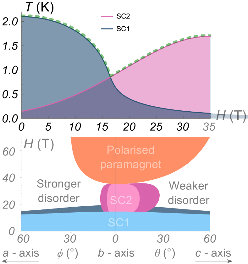
Figure 9: (a) Magnetic field dependence of critical temperatures for superconducting phases SC1 and SC2 for $\mathbf{H}$ oriented along the $b-$axis estimated from Eq. (4). We used $T_{c}=2.1$ K, $\mu_{e}=0.2\mu_{\text{B}}$, $c(0)=0.7$ for SC1 (see Eq. (5)) and $\Lambda=1.5$ K, $\frac{8M_{*}^{2}\nu\kappa}{g^{2}}=500$, $H_{m}=35$ T for SC2. The green dashed line is an envelope of the two transition lines that is measured experimentally. (b) Calculated angular magnetic field phase diagram. The color coding is the same as for the experimental phase diagram in Fig. 8. The MM phase transition is obtained from Eq. (2) and is well fit with $\chi^{-1}_{y}=1$, $\chi^{-1}_{z}=0.5$, $\chi^{-1}_{x}=0.01$, $\beta_{xx}=0.02$, $\beta_{yy}=-2$, $\beta_{zz}=2$, $\beta_{xy}=20$, and $\gamma=0.8$ (all other parameters set to zero), with magnetic field measured in Tesla. For SC1, we took $c=0.7+0.1\sin^{2}\theta$, $T=0.35$ K ($0.035$ K) and $\Gamma_{e}=0$ ($0.2$) to model the clean (dirty) sample. (We neglect the anisotropy of $H_{c}$ seen in experiment in this case.) For SC2 we use Eq. (4) with $\Omega_{*}$ from Eq. (3), with resulting parameters $H_{m}=35$ T, $g=1.6\times 10^{-3}$ and $\alpha=0.024$. For the metamagnon decay rate $\Gamma_{m}=\gamma_{x}\sin^{4}\phi+\gamma_{z}\sin^{4}\theta$, we took $\gamma_{x}=0.4$ and $\gamma_{z}=0.007$ to model the MSF samples and $\gamma_{x}=4$ and $\gamma_{z}=0.07$ to model the CVT samples (i.e. $\Gamma_{m}(\text{CVT})=10\Gamma_{m}(\text{MSF})$), and we took $T=0.1$ K. A good agreement with experimental data is observed for both panels.

For any form of the parameter, the critical temperature for SC2 is given by

$$T_{c}^{(SC2)}(\mathbf{H})=1.13\Lambda\exp\left[-\frac{\left(\Omega^{2}_{*}(0)+\Gamma_{m}^{2}\right)^{2}}{8\nu\tilde{\kappa}\mu_{e}^{2}M_{*}^{2}\Omega^{2}_{*}(0)}\right],$$ (4)

where $\nu$ is the density of states, $\Lambda$ is the energy cutoff, and $\tilde{\kappa}$ is equal to the largest $\kappa_{j}$ times some form factor with units of momentum squared coming from integration over momentum. The corresponding $T_{c}$ vs $H_{y}$ plot is shown in Fig. 9(a), which also shows a cartoon picture of $T_{c}^{(SC1)}$ in the SC1 phase. Importantly, we assume that SC1 is driven by some spin fluctuations that do not involve the metamagnon and have a strength that is independent of the applied field. We model the corresponding critical temperature for the SC1 phase as

$$\log\frac{T_{c}^{(SC1)}}{T_{c0}^{(SC1)}}=-(1-c(\theta,\phi))F\left(\frac{\Gamma_{e}}{T_{c}}\right)-c(\theta,\phi)F\left(\frac{\Gamma_{e}+ih}{T_{c}}\right)$$ (5)

with $F(x)=\text{Re}\left[\psi\left(\frac{1}{2}+\frac{x}{2\pi}\right)-\psi\left(\frac{1}{2}\right)\right]$, where $h=\mu_{e}H=\mu_{\text{B}}g_{e}H/2$, $T_{c0}^{(SC1)}$ is the critical temperature of SC1 without disorder in zero magnetic field (that we take to be $2.1$ K), $0<c<1$ is a phenomenological form factor that depends on the direction of the applied field, $\Gamma_{e}$ is the electron decay rate due to disorder, and $\psi(x)$ is the digamma function. We derive this equation under the assumption that pairing is mediated by generic spin fluctuations that are insensitive to the applied field, with some further simplifying assumptions (see Appendix C). Note that in Fig. 9(a) we extrapolated Eq. (4) all the way up to $H_{y}=H_{m}$, though the formula is not strictly valid at that point as the coupling becomes strong.

In modelling the effects of disorder, we find that it is crucial that the metamagnon decay rate $\Gamma_{m}$ depends on the direction of the applied magnetic field, in particular if the decay is dominated by two magnon scattering and/or Gilbert damping processes [60, 61, 62]. The exact functional form depends on the precise decay mechanism, but we find phenomenologically that the data is well described with $\Gamma_{m}=\gamma_{x}\sin^{4}\phi+\gamma_{z}\sin^{4}\theta$, where $\phi$ and $\theta$ are the angles between the direction of magnetic field and the $b-$axis in the $ab-$ and $bc-$crystallographic planes, respectively. The resulting phase diagram in Fig. 9(b) is in good qualitative agreement with the experimental data.

Here we neglected several other effects that give SC2 additional dependence on the direction and strength of the magnetic field. First, fields pointing away from the $b$-axis have a component parallel to the $\mathbf{d}$-vector, and therefore suppress SC2; we find, however, that this effect does not significantly alter the phase diagram. Second, the magnetization $\mathbf{M}_{*}$ of the polarized paramagnetic phase is itself a function of the applied field and changes both magnitude and direction, which in turn alters the direction of the $\mathbf{d}$-vector. Third, we have neglected any mixing between SC1 and SC2, which necessarily occurs due to the breaking of crystalline symmetries by fields aligned away from the $b$-axis. And finally, we assumed the high energy cutoff is independent of the applied field, though it is likely a function of $\Omega_{*}$.

VII Discussion and outlook

It is likely that a significant contributory factor to the enhancement of $T_{\text{c}}$ for MSF-grown UTe₂ is the minimization of uranium vacancies. Recent x-ray diffraction (XRD) studies on UTe₂ specimens of varying quality found that CVT samples with 1.5 K $\leq T_{\text{c}}\leq$ 2.0 K possessed uranium site defects of between $\approx 1$-$3\%$, while low quality samples that did not exhibit (SC1) superconductivity at temperatures down to 0.45 K showed uranium vacancies of $\approx 4$-$5\%$ [28, 63, 40]. By contrast, an MSF specimen with $T_{\text{c}}=$ 2.1 K exhibited no uranium deficiency within the experimental resolution of the XRD instrument [28].

Therefore, the enhancement of $T_{\text{c}}(H)$ of the SC1 phase for field applied along each crystallographic direction, as reported for measurements of MSF samples in ref. [33] and reproduced here in Section III, is likely to be due to the minimization of uranium site vacancies for this alternative growth process utilizing a salt flux. Our striking observation of the enhanced angular profile of the SC2 phase, which we detailed in Sections IV & V, can be very well described by considering the effects of disorder on MM fluctuations, as we outlined in Section VI.

It has been proposed in ref. [19] that the SC2 phase may be spin-singlet in character, rather than spin-triplet as widely considered by other studies [54, 52, 53, 11, 58, 64, 65, 46, 45]. The authors of ref. [19] argue in favor of a singlet pairing mechanism for SC2 based on the profile of their high field specific heat measurements performed on CVT specimens. However, recent NMR measurements up to applied field strengths of 24.8 T argue strongly in favor of SC1 and SC2 both being spin-triplet [53]. Interestingly, the field dependence of the ¹²⁵Te-NMR intensity reported in ref. [53] indicates that in the SC1 phase the dominant spin component of the triplet pair points along the $a$-axis, while measurements at higher fields show that in the SC2 state the spins are instead aligned along the $b$-axis. This scenario is fully consistent with our MM fluctuation model presented in Section VI. We note that the broader profile of the SC2 superconducting transition (compared to that of SC1) observed in specific heat measurements in ref. [19] fits this picture of strong magnetic fluctuations near $H_{m}$ driving the formation of the SC2 phase, with the broader heat capacity anomaly being analogous to prior studies of superconducting states driven by nematic fluctuations [66, 67]. Indeed, such a profile of a broad specific heat anomaly for magnetic fluctuation-induced field-reinforced superconductivity has recently been considered for the case of the ferromagnetic superconductor URhGe [55]. More empirical guidance, particularly from thermodynamic probes, is urgently needed to carefully unpick the microscopics underpinning the remarkable magnetic field-reinforced SC2 superconducting phase of UTe₂.

An interesting question posed by the observation of higher $T_{\text{c}}(H)$ for the SC1 phase of MSF UTe₂, and the purity-driven enhancement of the angular range of the SC2 phase, concerns the dependence of the SC3 state on the crystalline disorder. It has recently been observed that a very low quality sample with a RRR of 7.5, which does not exhibit SC1 superconductivity down to $T\approx$ 0.5 K, nevertheless exhibits SC3 superconductivity at high magnetic fields [68]. This robustness to disorder of the SC3 phase implies that it is likely very different in character to the SC2 phase, which as we showed in Section IV is highly sensitive to crystalline quality.

Since the optimization of the MSF growth technique for high quality UTe₂ specimens in 2022 [28], a number of experiments on this new generation of samples have helped clarify important physical properties of this system. These include dHvA and SdH effect measurements that reveal the Fermi surface geometry [24, 25], NMR and thermal conductivity measurements that give strikingly different results to prior CVT studies [69, 70] – providing a new perspective on the possible gap symmetry – along with Kerr rotation and specific heat measurements that also differ from prior observations and interpretations of studies on CVT specimens [26, 11]. We are therefore hopeful that continued experimental investigation of this new generation of higher quality crystals will provide the empirical impetus to enable more detailed theoretical models of this intriguing material to soon be attained.

In summary, we have performed a detailed comparative study of UTe₂ crystals grown by the molten salt flux (MSF) and chemical vapor transport (CVT) techniques. We found that the higher critical temperatures and lower residual resistivities of our ultraclean MSF crystals translated into higher critical field values compared to prior CVT studies. Comparatively, the properties of the metamagnetic (MM) transition, located at $\mu_{0}H_{m}\approx 35$ T for $H\parallel b$, appeared the same for both types of samples. This implies that the MM transition is a robust feature of the UTe₂ system that is insensitive to crystalline disorder, unlike the superconductivity. Strikingly, we found that the magnetic field-reinforced superconducting state close to this MM transition (SC2) has a significantly enhanced angular range for the cleaner MSF crystals. This observation can be well described by considering the enhanced role of magnetic fluctuations in proximity to the MM transition, thereby underpinning this intriguing field-reinforced superconducting phase, which is then quenched upon passing through the MM transition. This interpretation is consistent with recent NMR measurements, which taken together strongly imply that the field-reinforced phase (SC2) is markedly different in character compared to the zero-field superconducting state (SC1).

Appendix A SAMPLE CHARACTERIZATION AND CALIBRATION

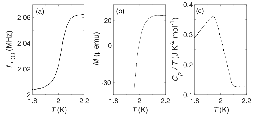
Figure 10: Superconducting transition of the sample measured to high fields in Fig. 4, measured at ambient magnetic field. The superconducting transition was measured by (a) PDO, (b) SQUID, and (c) heat capacity.

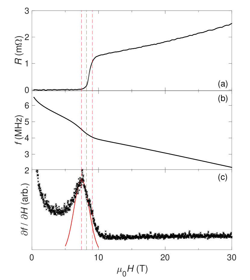
Figure 11: Simultaneous measurement of (a) contacted resistivity and (b) contactless resistivity performed on the same sample. The derivative of the contactless resistivity data is given in (c).

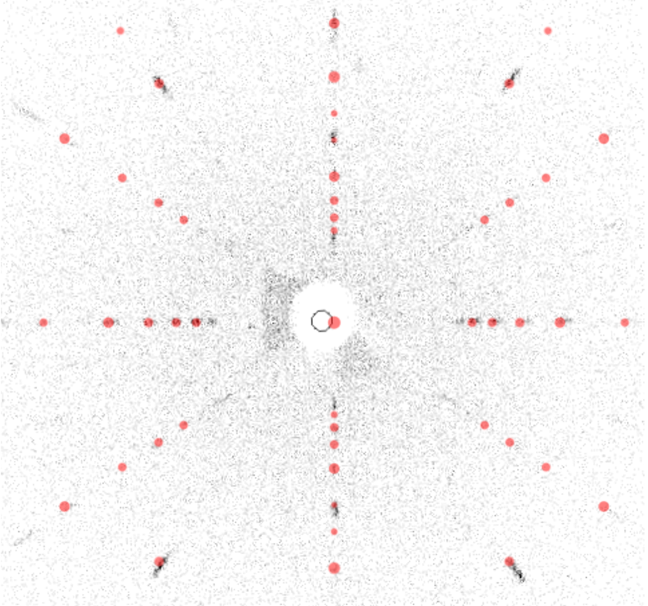
Figure 12: Lauegram of a UTe₂ sample (black and white), overlaid with the expected diffraction pattern for x-rays incident on the (001) plane (in red). Single crystallinity is evidenced, with the [001] direction aligned to within 1$\degree$.

In this section we compare characterization measurements of the sample measured by the PDO technique to high fields, for which the data are presented in Fig. 4. We measured the superconducting transition of this sample by three different methods: (a) PDO, (b) superconducting quantum interference device (dc SQUID), and (c) specific heat. PDO was measured by connecting the same coil as was later used in the 70 T pulsed magnet onto a homemade low temperature probe by a coaxial cable. This was then measured on cooling to the base temperature (1.8 K) of a PPMS system at 0.02 K/min in zero applied field. The dc magnetic moment, $M$, was measured by a QD Magnetic Property Measurement System (MPMS). The curve shown in Fig. 10(b) was measured on warming with a 10 Oe field applied after a zero-field cool-down. Heat capacity ($C_{p}$) was measured by a standard QD PPMS heat capacity module.

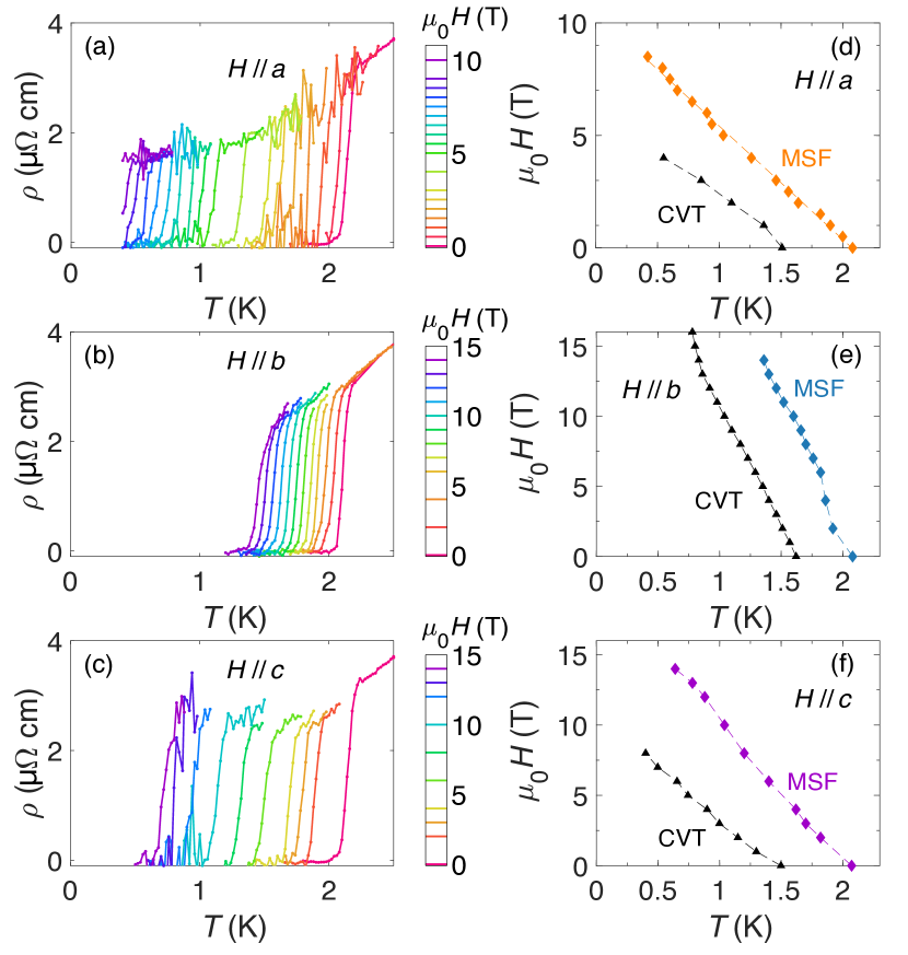
Figure 13: Resistivity curves as a function of temperature for the RRR = 406 sample from Table 1 at intermediate magnetic fields with $H$ applied along the (a) $a$-axis, (b) $b$-axis, and (c) $c$-axis. The strength of the applied field is indicated by the color scale. The corresponding profile of $T_{c}(H)$ is given in panels (d-f). A comparison is made between MSF-grown and CVT-grown $\mathrm{UTe}_{2}$ using CVT data points from ref. [10].

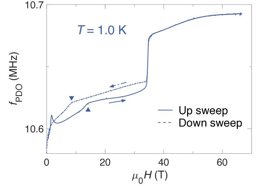
Figure 14: Comparison of pulsed field PDO data, with $H\parallel b$ at 1.0 K, for the up-sweep (solid) and down-sweep (dashed) of a magnetic field pulse. Arrows indicate the direction of field sweep, with markers indicating the anomalous kink feature displayed in Fig. 4(b). We note that the sharp feature at the start of the up-sweep is likely due to a flux line moving in the SC1 state – similar features have been observed in prior pulsed field studies of superconductors [14, 71, 72]. The overlap of the rising and falling traces is very good above 35 T in the field polarised state, which is known to have minimal temperature dependence around 1 K, but is noticeably different below 35 T when superconductivity returns, where the temperature dependence is much more sensitive. This observation is consistent with heating effects from eddy currents and/or vortex motion during the pulse.

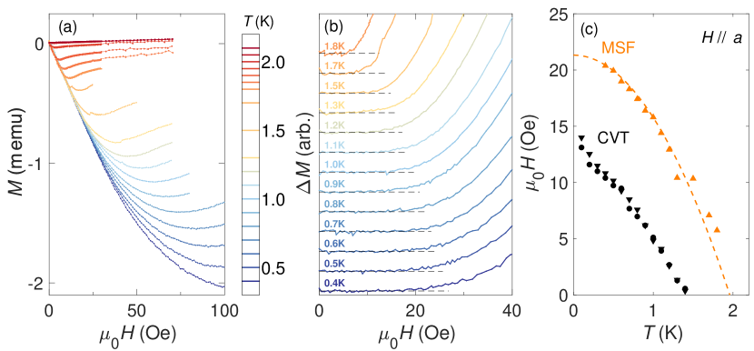
Figure 15: Magnetization measurements at low temperatures and magnetic fields. Measurements were performed on the RRR = 105 sample from Table 1. (a) Isothermal measurements of the dc magnetic moment, M, as a function of magnetic field strength for $H\parallel a$. Temperature points are indicated by the color scale. (b) Magnetic moment versus field after subtracting a linear fit to the data for $\mu_{0}H<5$ Oe, as described in the text. Each curve is offset for clarity. (c) Magnetic field–temperature phase diagram of the Meissner state of UTe₂ for $H\parallel a$. A comparison of CVT data is included from ref. [73].

Figure 11 shows contacted and contactless resistivity measurements performed simultaneously on the same sample. A Gaussian is fitted to the derivative, with dashed lines marking the location of the Gaussian midpoint, 0.5$\sigma$, and 1$\sigma$. We find in Fig. 2 that very good correspondence between PDO and contacted resistivity measurements is observed by empirically taking the Gaussian centre of the derivative of the PDO signal plus 0.5$\sigma$. The PDO error bars in Fig. 2 are each of length 1$\sigma$ (to represent an approximate uncertainty of $\pm$ 0.5$\sigma$).

Crystallographic orientation was calibrated by Laue diffraction as shown in Fig. 12. For pulsed field measurements, the data at 20$\degree$ and 33$\degree$ shown in Fig. 7 were obtained by mounting the sample on wedges of PEEK machined to the desired angles. The rotation study in dc magnetic fields presented in Fig. 5 was performed with a single-axis rotation probe utilizing a gear mechanism, with the rotation angle calibrated using a Hall sensor.

Appendix B PHASE MAPPING OF UTe₂

All contacted resistivity measurements to determine the upper critical field ($H_{c2}$) of the SC1 phase, presented as solid diamonds in Fig. 2, were obtained on the RRR = 406 sample from Table 1. This sample was oriented by Laue diffractometry and then securely mounted on a G10 sample board to enable easy orientation along each crystallographic axis. Figure 13 shows the raw data from which Fig. 2 is partly constructed. These data were obtained using the dc electrical transport module of a QD PPMS down to a base temperature of 0.5 K. Each data point was obtained by stabilizing the temperature and averaging over several measurements. $T_{c}(H)$ was defined by zero resistivity, which we identify as the first measurement point to fall below 0.1 $\upmu\Omega$ cm on cooling. The excitation current for measurements with field applied along the $a$- and $c$-axes was 100 $\upmu$A; the excitation current for measurements with field applied along the $b$-axis was 200 $\upmu$A. Small applied currents were required to maintain the temperature stability, due to low cooling power for $T\lessapprox$ 1 K.

Figure 14 shows the PDO signal for rising and falling magnetic field over the duration of a pulsed field measurement. Due to the high $\partial{H}/\partial{t}$ of a pulsed magnet, some amount of heating (from eddy currents and vortex motion) is inevitable [14, 71, 72]. On inspecting the up- and down-sweeps in Fig. 14, the location of the kink feature – which identifies the transition from SC1 to SC2 – has clearly moved to lower field on the down-sweep. This is highly likely to be an effect of heating during the pulse. Therefore, in Fig. 4 we use only the up-sweep data of each PDO measurement, to mitigate this effect.

Magnetization measurements to determine the lower critical field ($H_{c1}$) were obtained using the helium-3 option of a QD MPMS, for which the data are presented in Figure. 15. The sample was mounted inside a Kapton tube, with the field aligned along the $a$-axis. For each isothermal field sweep, the sample was first warmed up above its critical temperature and the magnet was turned off at high temperature. Then the sample was cooled down to the assigned temperature in zero field. dc magnetic moment measurements were then performed with stabilized magnetic field.

When a sample is in the Meissner phase, it will be in a diamagnetic state of constant susceptibility [74]. In terms of moment versus field, a straight line is thus expected within the Meissner state. The lower critical field may therefore be identified as the lowest field value where the $M$ vs $H$ curve deviates from linearity (with a correction for the demagnetization effect, as detailed in e.g. refs. [75, 76]). We fit a linear function to the data below 5 Oe at each temperature, which is then subtracted from each curve. The background-subtracted data for each temperature are shown in Fig. 15(b). The flux penetration field $H_{p}$ is then extracted by finding the first point that deviates from the flat line at each temperature. Following the discussion in ref. [77], $H_{c1}$ may be related to $H_{p}$ via the expression:

$$H_{c1}=\frac{H_{p}}{\tanh{\sqrt{0.36t/w}}},$$ (6)

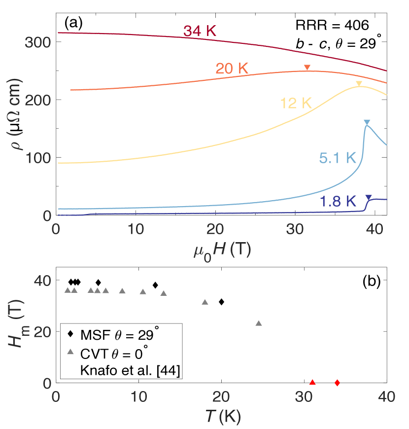
Figure 16: (a) dc field resistivity data tracking the evolution of the metamagnetic transition at $H_{m}$ (indicated with markers). (b) Comparison between the progression in temperature of $H_{m}$ from panel (a) with that reported for a CVT sample in ref. [44]. The red symbols indicate the first measured temperature point of each study at which the MM transition is no longer observed (which at elevated temperatures is identified as a broad maximum).

where $t$ is the sample thickness and $w$ is the sample width. For this measurement, with $H\parallel a$, $t=3.46$ mm (along the $a$ direction) and $w=0.51$ mm.

We find that $H_{c1}$ is enhanced for this new generation of higher quality samples (Fig. 15(c)), similar to the higher $H_{c2}$ values shown in Fig. 2. We note that the $H_{c1}$ value of $\approx$ 20 Oe we observe for $H\parallel a$ agrees well with a recent report of a similar study on MSF-grown UTe₂ [34].

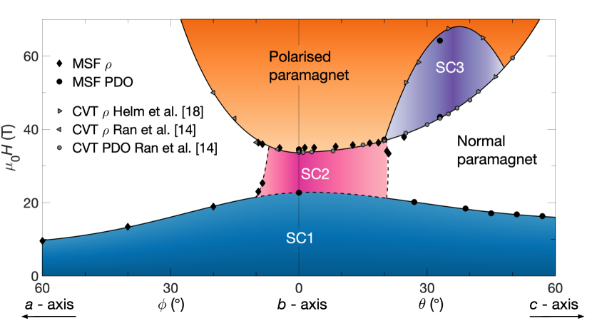
Figure 17: Angular magnetic field phase diagram for MSF-grown $\mathrm{UTe}_{2}$ for $\mu_{0}H\leq 70$ T. Lines are as a guide to the eye. Comparative data points from pulsed field studies on CVT samples are from refs. [14, 18].

Figure 4 shows the temperature evolution of the MM transition up to 3 K, over which interval it displays little change. We also tracked the evolution of $H_{m}$ to higher temperatures, as shown in Figure 16. Whereas at low temperature $H_{m}$ is very clearly visible by the sudden increase of the resistivity, at high temperatures this feature rounds out into a broad maximum, indicated with markers in Fig. 16(a).

In Fig.  16(b) we compare the temperature evolution of the MM transition between our study on a MSF sample with that reported previously in ref. [44] for a CVT specimen. Note that our study and that of ref.  [44] are performed at different angles, so the location of $H_{m}$ (at equivalent temperature) is slightly different. However, as we show in Figs. 7 & 8 the angular evolution of $H_{m}$ is the same for MSF and CVT samples. Furthermore, from the comparison in Fig. 16(b), it is clear that $H_{m}$ displays a very similar temperature dependence for both types of sample. This indicates that the energy scale of the MM transition is unchanged between the two types of samples. We note that the MM transition at $H_{m}$ is still observed even in very low quality samples that do not show SC1 superconductivity down to temperatures $\approx$ 0.5 K [68]. Given that we observe no change in the profile of this transition for this new generation of ultraclean crystals, we conclude that the MM transition is an intrinsic feature of the UTe₂ system, and unlike the superconductivity, is insensitive to the presence of crystalline disorder.

Appendix C DETAILS OF THEORETICAL CALCULATIONS

C.1 Model for SC2

Here we present the details of the derivation of the spin-fluctuation interactions by integrating out the metamagnons. The action is given by

$$\begin{gathered}\mathcal{S}=-\sum_{n,\mathbf{q}}(i\Omega_{n}-\Omega_{*}(\mathbf{q})+i\Gamma_{m}\mathcal{\text{sgn}}\Omega_{n})m^{\dagger}_{\mathbf{q}}m_{\mathbf{q}}+\\ +\sum_{\mathbf{q}}\mu_{e}(m_{\mathbf{q}}+m_{-\mathbf{q}}^{\dagger})M_{*}S_{\parallel}\end{gathered}$$ (7)

with $\Omega_{*}(\mathbf{q})$ given in Eq. (3) and where we use the Matsubara formalism; $\Omega_{n}=2\pi nT$ are bosonic Matsubara frequencies. We also introduced the decay term $\Gamma_{m}$ to account for the finite lifetime of the metamagnon. Here we assume that the metamagnon is a degree of freedom that stems from localized magnetic moments and not the itinerant fermionic degrees of freedom; this is consistent with recent theories of metamagnetic phase transitions in Kondo lattices [78, 79]. This assumption allows us to integrate the bosons out in the standard way, which gives an effective dimensionless action for the fermions

$$\mathcal{S}_{M}[c,c^{\dagger}]=\beta\sum_{n,\mathbf{q}}J(i\Omega_{n},\mathbf{q})S_{\parallel}(i\Omega_{n},\mathbf{q})S_{\parallel}(-i\Omega_{n},-\mathbf{q}),$$ (8)

where

$$J(i\Omega_{n},\mathbf{q})=-\frac{\mu_{e}^{2}M_{*}^{2}\Omega_{*}(\mathbf{q})}{\Omega^{2}_{*}(\mathbf{q})+\Omega_{n}^{2}+\Gamma_{m}^{2}}$$ (9)

are the effective ferromagnetic-fluctuation type interactions. This is equivalent to writing the interaction Hamiltonian as

$$\mathcal{H}_{int}=\sum_{n,\mathbf{q,k,p}}J(i\Omega_{n},\mathbf{q})c^{\dagger}_{\mathbf{k+q}s_{1}}\left(\bm{\sigma}\cdot\hat{\mathbf{M}}_{*}\right)_{s_{1}s_{2}}c_{\mathbf{k}s_{2}}c^{\dagger}_{\mathbf{p-q}s_{3}}\left(\bm{\sigma}\cdot\hat{\mathbf{M}}_{*}\right)_{s_{3}s_{4}}c_{\mathbf{p}s_{4}}.$$ (10)

A proper treatment of the frequency dependence of the interaction would require solving the Eliashberg equations [80, 81, 82]. However, because close to the metamagnetic phase transition the interaction strength has a similar frequency dependence as in the case of phonons, i.e., the attraction happens mostly at low frequency, we can approximate $J(i\Omega_{n},\mathbf{q})\approx J(0,\mathbf{q})$. This gives us the form of the interactions as stated in Section VI. We note that there are additional corrections due to the fact that the metamagnons, unlike phonons, are massive excitations away from the metamagnetic transition. This would likely modify the low energy cutoff of the theory in a more rigorous treatment, but the effect should be small close to the metamagnetic transition.

To get the gap equation and obtain the expression for $T_{c}$ we first need to recast the interaction in the singlet/triplet pairing channels using the Pauli matrix completeness relation

$$2\delta_{s_{1}s_{2}}\delta_{s_{3}s_{4}} =\sum_{\mu=0,x,y,z}\sigma^{\mu}_{s_{1}s_{3}}\sigma^{\mu}_{s_{2}s_{4}}=$$

$$=\sum_{\mu}(\sigma^{\mu}i\sigma^{y})_{s_{1}s_{3}}\left[(\sigma^{\mu}i\sigma^{y})^{\dagger}\right]_{s_{2}s_{4}}$$ (11)

that yields (using the four-momentum notation $p=(i\omega_{n},\mathbf{p})$ etc)

$$H_{int} =V_{\mu}(p;k)$$ (12)

$$\times\left(c^{\dagger}_{-ks_{1}}(\sigma^{\mu}i\sigma^{y})_{s_{1}s_{3}}c^{\dagger}_{ks_{3}}\right)\left(c_{ps_{4}}(\sigma^{\mu}i\sigma^{y})^{*}_{s_{4}s_{2}}c_{-ps_{2}}\right)$$

with $\mu=0$ and $\mu=j=x,y,z$ corresponding to singlet and triplet pairing channels respectively, where

$$V_{0}(p;k) =-J^{(S)}_{x}(p-k)-J^{(S)}_{y}(p-k)-J^{(S)}_{z}(p-k)$$

$$V_{x}(p;k) =-J^{(A)}_{x}(p-k)+J^{(A)}_{y}(p-k)+J^{(A)}_{z}(p-k)$$

$$V_{y}(p;k) =J^{(A)}_{x}(p-k)-J^{(A)}_{y}(p-k)+J^{(A)}_{z}(p-k)$$

$$V_{z}(p;k) =J^{(A)}_{x}(p-k)+J^{(A)}_{y}(p-k)-J^{(A)}_{z}(p-k)$$ (13)

and where $J^{(S/A)}_{j}=J^{(S/A)}(q)\hat{M}_{*j}$ is proportional to the $j^{th}$ component of $\hat{\mathbf{M}}_{*}$, with

$$J^{(S/A)}(p-k)=\frac{J(p-k)\pm J(p+k)}{2}\,.$$ (14)

The functions $J^{(S/A)}(p-k)$ can be decomposed into terms transforming according to particular irreducible representations of the crystalline point group symmetries. To leading order, this can be achieved by expanding $J^{(S/A)}(p-k)$ in momentum and keeping only the leading term. This yields

$$J^{(S)}(\mathbf{p-k}) \sim-\frac{\mu_{e}^{2}M_{*}^{2}\Omega_{*}(0)}{\Omega^{2}_{*}(0)+\Gamma_{m}^{2}},$$

$$J^{(A)}(\mathbf{p-k}) \sim-\frac{2\mu_{e}^{2}M_{*}^{2}\Omega_{*}^{2}(0)}{(\Omega^{2}_{*}(0)+\Gamma_{m}^{2})^{2}}\sum_{j}\kappa_{j}p_{j}k_{j}.$$ (15)

We next introduce the gap functions via a Hubbard-Stratonovich transformation:

$$H_{\Delta}=\sum\Delta^{(\mu)}(p)(\sigma^{\mu}i\sigma^{y})_{s_{1}s_{2}}c^{\dagger}_{ps_{1}}c^{\dagger}_{-ps_{2}}.$$ (16)

The corresponding linearized gap equation (valid in the weak coupling approximation) reads

$$\Delta^{(\mu)}(p)=-T\sum_{k}V_{\mu}(p;k)\Pi_{\mu\mu^{\prime}}(k)\Delta^{(\mu^{\prime})}(k)$$ (17)

where

$$\Pi_{\mu\mu^{\prime}}(k)=\text{Tr}\left[\sigma^{\mu}i\sigma^{y}G(k)(\sigma^{\mu^{\prime}}i\sigma^{y})^{*}G^{T}(-k)\right]$$ (18)

is the particle-particle bubble (before the Matsubara sum), the trace is over spin indices, and

$$G(k) =\frac{1}{i\omega_{n}-\varepsilon(\mathbf{k})-\mu_{e}\mathbf{H}\cdot\bm{\sigma}}=$$ (19)

$$=\frac{i\omega_{n}-\varepsilon(\mathbf{k})+\mu_{e}\mathbf{H}\cdot\bm{\sigma}}{(i\omega_{n}-\varepsilon(\mathbf{k}))^{2}-\mu_{e}^{2}H^{2}}$$

is the Green’s function that includes the Zeeman term.

For the special case of $\mathbf{H}$ along the $y$ axis, since we can assume that the Fermi surfaces are spin polarized close to the phase transition, we take $G(k)\propto\frac{1}{2}(\pm 1+\sigma^{y})$ (with $\pm$ corresponding to the two spin split Fermi surfaces). One can then check that the $\mu=0,y$ channels vanish while

$$\Pi_{xx}(k)=\Pi_{zz}(k)=\frac{1}{\omega_{n}^{2}-(\varepsilon(\mathbf{k})\pm\mu_{e}H)^{2}}$$

$$\Pi_{xz}(k)=\pm\Pi_{zx}(k)=\frac{i}{\omega_{n}^{2}-(\varepsilon(\mathbf{k})\pm\mu_{e}H)^{2}}$$ (20)

with the $\pm$ in the denominator corresponding to the Fermi surface with spin aligned against and with the magnetic field, respectively. Note that the relevant interactions are thus $V_{x}=V_{z}=J_{y}^{(A)}$, so that the $\mathbf{d}=d(1,0,\pm i)$ vector is interestingly non-unitary, similar to that proposed in [59].

Combining with our knowledge of the $\mathbf{d}$-vector, we obtain the final equation for $\Delta$ with $\Delta^{(x)}(\mathbf{k})=-i\Delta^{(z)}(\mathbf{k})=\Delta(\mathbf{k})$ (summing over both spin polarized Fermi surfaces for additional factor of two, another factor of two from the eigenvalue of $\Pi$ matrix, and neglecting form factors from Fermi surface shapes):

$$\Delta(\mathbf{p})=\frac{8\nu\mu_{e}^{2}M_{*}^{2}\Omega_{*}^{2}(0)}{(\Omega^{2}_{*}(0)+\Gamma_{m}^{2})^{2}}\log\frac{1.13\Lambda}{T_{c}}\sum_{j}\kappa_{j}\int p_{j}k_{j}\Delta(\mathbf{k})dS_{FS}$$ (21)

where the surface integral is taken over the Fermi surface. The solutions are thus $\Delta(\mathbf{p})\propto p_{j}$, with different $j$ belonging to different irreps. Possibilities include the $B_{1u}+iB_{3u}$ irrep combination of $D_{2h}$ irrep for $j=y$ (corresponding to the $B_{u}$ irrep of $C_{2h}$ in the presence of a magnetic field along the $b$ axis) as proposed in [59]; or, for either $j=x$ or $j=z$, the $A_{u}+iB_{2u}$ combination ($A_{u}$ irrep of $C_{2h}$) that was considered in [52]. Regardless of the form of the order parameter, within weak coupling we obtain an expression for $T_{c}$ in Eq. (4) with a parameter $\kappa$ that accounts for any form factors resulting from the integration over the Fermi surface. As the form of the order parameter is still under debate, we simply consider $\kappa$ as a phenomenological parameter.

C.2 Model for SC1

To model SC1, let us assume that the FM (or AFM) fluctuation-induced interaction at zero external field has the form

$$H_{int} =V\left(c^{\dagger}_{-ks_{1}}(\hat{\mathbf{d}}(\mathbf{k})\cdot\bm{\sigma}i\sigma^{y})_{s_{1}s_{3}}c^{\dagger}_{ks_{3}}\right)\left(c_{ps_{4}}(\hat{\mathbf{d}}(\mathbf{p})\cdot\bm{\sigma}i\sigma^{y})^{*}_{s_{4}s_{2}}c_{-ps_{2}}\right)$$ (22)

where $V$ is a constant. Unlike the SC2 model, here we assume that $V$ is independent of the applied field and arises from intrinsic spin fluctuations present in the ground state of the system in the absence of any field. It is then easy to see that the self-consistent gap functions have the form $\Delta(\mathbf{p})=\mathbf{d}(\mathbf{k})\cdot\bm{\sigma}i\sigma^{y}$. For simplicity, let us quantize spin along the direction of $\mathbf{H}$, so that

$$G(k)=\left(\begin{array}[]{cc}\frac{1}{i\omega_{n}-\varepsilon(\mathbf{k})-h+i\Gamma_{e}\mathcal{\text{sgn}}\omega_{n}}&0\\ 0&\frac{1}{i\omega_{n}-\varepsilon(\mathbf{k})+h+i\Gamma_{e}\mathcal{\text{sgn}}\omega_{n}}\end{array}\right)\equiv\left(\begin{array}[]{cc}G_{\uparrow}(k)&0\\ 0&G_{\downarrow}(k)\end{array}\right)$$ (23)

where $h=\mu_{e}H=\mu_{B}g_{e}H/2$ and we introduced the electron decay rate $\Gamma_{e}$ to account for disorder. Evaluating the trace we then obtain the following self-consistency gap equation (cf. [83, 84]):

$$1=-VT\sum_{\mathbf{k}}\left[(|d_{x}(\mathbf{k})|^{2}+|d_{y}(\mathbf{k})|^{2})(G_{\uparrow}(k)G_{\uparrow}(-k)+G_{\downarrow}(k)G_{\downarrow}(-k))+|d_{z}(\mathbf{k})|^{2}(G_{\uparrow}(k)G_{\downarrow}(-k)+G_{\uparrow}(-k)G_{\downarrow}(k))\right].$$ (24)

We can generalize to any orientation of the magnetic field by using a coordinate-free notation:

$$1=-VT\sum_{\mathbf{k}}\left[|d_{\perp}(\mathbf{k})|^{2}(G_{\uparrow}(k)G_{\uparrow}(-k)+G_{\downarrow}(k)G_{\downarrow}(-k))+|d_{\parallel}(\mathbf{k})|^{2}(G_{\uparrow}(k)G_{\downarrow}(-k)+G_{\uparrow}(-k)G_{\downarrow}(k))\right].$$ (25)

The Matsubara sums for the $d_{\perp}$ part are the same as without magnetic field (these components are thus insensitive to the magnetic field), and in the absence of disorder we obtain the usual logarithmic term. With disorder, we get

$$\sum_{n}\int d\varepsilon G_{\uparrow}(k)G_{\uparrow}(-k)=\sum_{n}\int d\varepsilon G_{\downarrow}(k)G_{\downarrow}(-k)=\log\frac{1.13\Lambda}{T}-\psi\left(\frac{1}{2}+\frac{\Gamma_{e}}{2\pi T}\right)+\psi\left(\frac{1}{2}\right).$$ (26)

Evaluating the sum for the $d_{\parallel}$ term, on the other hand, gives (assuming $h\ll\Lambda$)

$$\sum_{n}\int d\varepsilon G_{\uparrow}(k)G_{\downarrow}(-k)=\log\frac{1.13\Lambda}{T}-\text{Re}\left[\psi\left(\frac{1}{2}+\frac{\Gamma_{e}+ih}{2\pi T}\right)-\psi\left(\frac{1}{2}\right)\right]$$ (27)

where $\psi$ is the digamma function. After doing the sum over $\mathbf{k}$ in Eq. (25), we then have

$$1=-\tilde{V}\left[\log\frac{1.13\Lambda}{T}-(1-c(\theta,\phi))\left[\psi\left(\frac{1}{2}+\frac{\Gamma_{e}}{2\pi T}\right)-\psi\left(\frac{1}{2}\right)\right]-c(\theta,\phi)\text{Re}\left[\psi\left(\frac{1}{2}+\frac{\Gamma_{e}+ih}{2\pi T}\right)-\psi\left(\frac{1}{2}\right)\right]\right]$$

with

$$\tilde{V}=2V\nu\int|\mathbf{d}(\mathbf{k})|^{2}dS_{FS}$$

and

$$0<c(\theta,\phi)=\frac{\int|d_{\parallel}(\mathbf{k})|^{2}dS_{FS}}{\int|\mathbf{d}(\mathbf{k})|^{2}dS_{FS}}<1$$

is a form factor that we can treat as a phenomenological parameter that only depends on the direction of the field $\mathbf{H}$. This is most conveniently re-written as

$$\log\frac{T_{c}(\mathbf{H},\Gamma_{e})}{T_{c0}}=-(1-c(\theta,\phi))F\left(\frac{\Gamma_{e}}{T_{c}}\right)-c(\theta,\phi)F\left(\frac{\Gamma_{e}+ih}{T_{c}}\right)$$

where $F(x)=\text{Re}\left[\psi\left(\frac{1}{2}+\frac{x}{2\pi}\right)-\psi\left(\frac{1}{2}\right)\right]$, leading to the expression in the main text that was used to obtain the plots in Fig. 9.

References

- Bardeen et al. [1957] J. Bardeen, L. N. Cooper, and J. R. Schrieffer, Theory of Superconductivity, Phys. Rev. 108, 1175 (1957).
- Cooper [1956] L. N. Cooper, Bound Electron Pairs in a Degenerate Fermi Gas, Phys. Rev. 104, 1189 (1956).
- Monthoux et al. [2007] P. Monthoux, D. Pines, and G. G. Lonzarich, Superconductivity without phonons, Nature 450, 1177 (2007).
- Norman [2011] M. R. Norman, The Challenge of Unconventional Superconductivity, Science 332, 196 (2011).
- Stewart [2017] G. R. Stewart, Unconventional superconductivity, Adv. Phys. 66, 75 (2017).
- Saxena et al. [2000] S. S. Saxena, P. Agarwal, K. Ahilan, F. M. Grosche, R. K. W Haselwimmer, M. J. Steiner, E. Pugh, I. R. Walker, S. R. Julian, P. Monthoux, G. G. Lonzarich, A. Huxley, I. Sheikin, D. Braithwaite, and J. Flouquet, Superconductivity on the border of itinerant-electron ferromagnetism in UGe2, Nature 406, 587 (2000).
- Aoki et al. [2001] D. Aoki, A. Huxley, E. Ressouche, D. Braithwaite, J. Flouquet, J. P. Brison, E. Lhotel, and C. Paulsen, Coexistence of superconductivity and ferromagnetism in URhGe, Nature 413, 613 (2001).
- Huy et al. [2007] N. T. Huy, A. Gasparini, D. E. de Nijs, Y. Huang, J. C. P. Klaasse, T. Gortenmulder, A. de Visser, A. Hamann, T. Görlach, and H. v. Löhneysen, Superconductivity on the Border of Weak Itinerant Ferromagnetism in UCoGe, Phys. Rev. Lett. 99, 067006 (2007).
- Aoki et al. [2019a] D. Aoki, K. Ishida, and J. Flouquet, Review of U-based Ferromagnetic Superconductors: Comparison between UGe2, URhGe, and UCoGe, J. Phys. Soc. Jpn. 88, 022001 (2019a).
- Ran et al. [2019a] S. Ran, C. Eckberg, Q. P. Ding, Y. Furukawa, T. Metz, S. R. Saha, I. L. Liu, M. Zic, H. Kim, J. Paglione, and N. P. Butch, Nearly ferromagnetic spin-triplet superconductivity, Science 365, 684 (2019a).
- Aoki et al. [2022a] D. Aoki, J. P. Brison, J. Flouquet, K. Ishida, G. Knebel, Y. Tokunaga, and Y. Yanase, Unconventional superconductivity in UTe2, J. Phys. Condens. Matter 34, 243002 (2022a).
- Chandrasekhar [1962] B. Chandrasekhar, A note on the maximum critical field of high-field superconductors, Appl. Phys. Lett. 1, 7 (1962).
- Clogston [1962] A. M. Clogston, Upper Limit for the Critical Field in Hard Superconductors, Phys. Rev. Lett. 9, 266 (1962).
- Ran et al. [2019b] S. Ran, I. L. Liu, Y. S. Eo, D. J. Campbell, P. M. Neves, W. T. Fuhrman, S. R. Saha, C. Eckberg, H. Kim, D. Graf, F. Balakirev, J. Singleton, J. Paglione, and N. P. Butch, Extreme magnetic field-boosted superconductivity, Nat. Phys. 15, 1250 (2019b).
- Knebel et al. [2019] G. Knebel, W. Knafo, A. Pourret, Q. Niu, M. Vališka, D. Braithwaite, G. Lapertot, M. Nardone, A. Zitouni, S. Mishra, I. Sheikin, G. Seyfarth, J. P. Brison, D. Aoki, and J. Flouquet, Field-Reentrant Superconductivity Close to a Metamagnetic Transition in the Heavy-Fermion Superconductor , J. Phys. Soc. Jpn. 88, 63707 (2019).
- Knafo et al. [2021] W. Knafo, M. Nardone, M. Vališka, A. Zitouni, G. Lapertot, D. Aoki, G. Knebel, and D. Braithwaite, Comparison of two superconducting phases induced by a magnetic field in UTe2, Commun. Phys. 4, 40 (2021).
- Schönemann et al. [2022] R. Schönemann, P. F. S. Rosa, S. M. Thomas, Y. Lai, D. N. Nguyen, J. Singleton, E. L. Brosha, R. D. McDonald, V. Zapf, B. Maiorov, and M. Jaime, Thermodynamic evidence for high-field bulk superconductivity in UTe2 (2022), arXiv:2206.06508 .
- Helm et al. [2022] T. Helm, M. Kimata, K. Sudo, A. Miyata, J. Stirnat, T. Förster, J. Hornung, M. König, I. Sheikin, A. Pourret, G. Lapertot, D. Aoki, J.-P. Brison, G. Knebel, and J. Wosnitza, Suppressed magnetic scattering sets conditions for the emergence of 40 T high-field superconductivity in UTe2 (2022), arXiv:2207.08261 .
- Rosuel et al. [2023] A. Rosuel, C. Marcenat, G. Knebel, T. Klein, A. Pourret, N. Marquardt, Q. Niu, S. Rousseau, A. Demuer, G. Seyfarth, G. Lapertot, D. Aoki, D. Braithwaite, J. Flouquet, and J. P. Brison, Field-Induced Tuning of the Pairing State in a Superconductor, Phys. Rev. X 13, 011022 (2023).
- Hayes et al. [2021] I. M. Hayes, D. S. Wei, T. Metz, J. Zhang, Y. S. Eo, S. Ran, S. R. Saha, J. Collini, N. P. Butch, D. F. Agterberg, A. Kapitulnik, and J. Paglione, Multicomponent superconducting order parameter in UTe2, Science 373, 797 (2021).
- Thomas et al. [2020] S. M. Thomas, F. B. Santos, M. H. Christensen, T. Asaba, F. Ronning, J. D. Thompson, E. D. Bauer, R. M. Fernandes, G. Fabbris, and P. F. Rosa, Evidence for a pressure-induced antiferromagnetic quantum critical point in intermediate-valence UTe2, Sci. Adv. 6, 8709 (2020).
- Thomas et al. [2021] S. M. Thomas, C. Stevens, F. B. Santos, S. S. Fender, E. D. Bauer, F. Ronning, J. D. Thompson, A. Huxley, and P. F. S. Rosa, Spatially inhomogeneous superconductivity in , Phys. Rev. B 104, 224501 (2021).
- Rosa et al. [2022] P. F. S. Rosa, A. Weiland, S. S. Fender, B. L. Scott, F. Ronning, J. D. Thompson, E. D. Bauer, and S. M. Thomas, Single thermodynamic transition at 2 K in superconducting UTe2 single crystals, Commun. Mater. 3, 33 (2022).
- Aoki et al. [2022b] D. Aoki, S. Hironori, O. Petr, T. Yoshifumi, I. Jun, Y. Youichi, H. Hisatomo, N. Ai, L. Dexin, H. Yoshiya, S. Yusei, K. Georg, F. Jacques, and H. Yoshinori, First Observation of the de Haas–van Alphen Effect and Fermi Surfaces in the Unconventional Superconductor UTe2, J. Phys. Soc. Jpn. 91, 083704 (2022b).
- Eaton et al. [2023] A. G. Eaton, T. I. Weinberger, N. J. M. Popiel, Z. Wu, A. J. Hickey, A. Cabala, J. Pospíšil, J. Prokleška, T. N. Haidamak, G. Bastien, P. Opletal, H. Sakai, Y. Haga, R. Nowell, S. M. Benjamin, V. Sechovský, G. G. Lonzarich, F. M. Grosche, and M. Vališka, Quasi-2D Fermi surface in the anomalous superconductor (2023), arXiv:2302.04758 .
- Ajeesh et al. [2023] M. Ajeesh, M. Bordelon, C. Girod, S. Mishra, F. Ronning, E. Bauer, B. Maiorov, J. Thompson, P. Rosa, and S. Thomas, The fate of time-reversal symmetry breaking in UTe2 (2023), arXiv:2305.00589 .
- Haga et al. [1998] Y. Haga, T. Honma, E. Yamamoto, H. Ohkuni, Y. Ōnuki, M. Ito, and N. Kimura, Purification of Uranium Metal using the Solid State Electrotransport Method under Ultrahigh Vacuum, Jpn. J. Appl. Phys. 37, 3604 (1998).
- Sakai et al. [2022] H. Sakai, P. Opletal, Y. Tokiwa, E. Yamamoto, Y. Tokunaga, S. Kambe, and Y. Haga, Single crystal growth of superconducting by molten salt flux method, Phys. Rev. Mater. 6, 073401 (2022).
- Altarawneh et al. [2009] M. M. Altarawneh, C. H. Mielke, and J. S. Brooks, Proximity detector circuits: An alternative to tunnel diode oscillators for contactless measurements in pulsed magnetic field environments, Rev. Sci. Inst. 80, 066104 (2009).
- Ghannadzadeh et al. [2011] S. Ghannadzadeh, M. Coak, I. Franke, P. Goddard, J. Singleton, and J. L. Manson, Measurement of magnetic susceptibility in pulsed magnetic fields using a proximity detector oscillator, Rev. Sci. Inst. 82, 113902 (2011).
- Aoki et al. [2019b] D. Aoki, A. Nakamura, F. Honda, D. X. Li, Y. Homma, Y. Shimizu, Y. J. Sato, G. Knebel, J. P. Brison, A. Pourret, D. Braithwaite, G. Lapertot, Q. Niu, M. Vališka, H. Harima, and J. Flouquet, Unconventional Superconductivity in Heavy Fermion UTe2, J. Phys. Soc. Jpn. 88, 43702 (2019b).
- Sakai et al. [2023] H. Sakai, Y. Tokiwa, P. Opletal, M. Kimata, S. Awaji, T. Sasaki, D. Aoki, S. Kambe, Y. Tokunaga, and Y. Haga, Field Induced Multiple Superconducting Phases in along Hard Magnetic Axis, Phys. Rev. Lett. 130, 196002 (2023).
- Tokiwa et al. [2022] Y. Tokiwa, P. Opletal, H. Sakai, K. Kubo, E. Yamamoto, S. Kambe, M. Kimata, S. Awaji, T. Sasaki, D. Aoki, Y. Tokunaga, and Y. Haga, Stabilization of superconductivity by metamagnetism in an easy-axis magnetic field on UTe2 (2022), arXiv:2210.11769 .
- Ishihara et al. [2023] K. Ishihara, M. Kobayashi, K. Imamura, M. Konczykowski, H. Sakai, P. Opletal, Y. Tokiwa, Y. Haga, K. Hashimoto, and T. Shibauchi, Anisotropic enhancement of lower critical field in ultraclean crystals of spin-triplet superconductor candidate , Phys. Rev. Res. 5, L022002 (2023).
- Mackenzie et al. [1998] A. P. Mackenzie, R. K. W. Haselwimmer, A. W. Tyler, G. G. Lonzarich, Y. Mori, S. Nishizaki, and Y. Maeno, Extremely Strong Dependence of Superconductivity on Disorder in , Phys. Rev. Lett. 80, 161 (1998).
- Rullier-Albenque et al. [2003] F. Rullier-Albenque, H. Alloul, and R. Tourbot, Influence of pair breaking and phase fluctuations on disordered high cuprate superconductors, Phys. Rev. Lett. 91, 047001 (2003).
- Bauer et al. [2006] E. D. Bauer, F. Ronning, C. Capan, M. J. Graf, D. Vandervelde, H. Q. Yuan, M. B. Salamon, D. J. Mixson, N. O. Moreno, S. R. Brown, J. D. Thompson, R. Movshovich, M. F. Hundley, J. L. Sarrao, P. G. Pagliuso, and S. M. Kauzlarich, Thermodynamic and transport investigation of , Phys. Rev. B 73, 245109 (2006).
- Chen et al. [2019] J. Chen, M. B. Gamża, K. Semeniuk, and F. M. Grosche, Composition dependence of bulk superconductivity in , Phys. Rev. B 99, 020501 (2019).
- Abrikosov and Gor’kov [1960] A. A. Abrikosov and L. P. Gor’kov, Contribution to the Theory of Superconducting Alloys with Paramagnetic Impurities, J. Exptl. Theoret. Phys. 39 (1960).
- Weiland et al. [2022] A. Weiland, S. Thomas, and P. Rosa, Investigating the limits of superconductivity in UTe2, J. Phys. Mater. 5, 044001 (2022).
- Shoenberg [1984] D. Shoenberg, Magnetic Oscillations in Metals (Cambridge University Press, Cambridge, UK, 1984).
- Miyake et al. [2021] A. Miyake, Y. Shimizu, Y. J. Sato, D. Li, A. Nakamura, Y. Homma, F. Honda, J. Flouquet, M. Tokunaga, and D. Aoki, Enhancement and Discontinuity of Effective Mass through the First-Order Metamagnetic Transition in , J. Phys. Soc. Jpn. 90, 103702 (2021).
- Miyake et al. [2019] A. Miyake, Y. Shimizu, Y. J. Sato, D. Li, A. Nakamura, Y. Homma, F. Honda, J. Flouquet, M. Tokunaga, and D. Aoki, Metamagnetic Transition in Heavy Fermion Superconductor , J. Phys. Soc. Jpn. 88 (2019).
- Knafo et al. [2019] W. Knafo, M. Vališka, D. Braithwaite, G. Lapertot, G. Knebel, A. Pourret, J.-P. Brison, J. Flouquet, and D. Aoki, Magnetic-field-induced phenomena in the paramagnetic superconductor , J. Phys. Soc. Jpn. 88, 063705 (2019).
- Shishidou et al. [2021] T. Shishidou, H. G. Suh, P. M. R. Brydon, M. Weinert, and D. F. Agterberg, Topological band and superconductivity in , Phys. Rev. B 103, 104504 (2021).
- Ishizuka et al. [2019] J. Ishizuka, S. Sumita, A. Daido, and Y. Yanase, Insulator-Metal Transition and Topological Superconductivity in from a First-Principles Calculation, Phys. Rev. Lett. 123, 217001 (2019).
- Shaffer and Chichinadze [2022] D. Shaffer and D. V. Chichinadze, Chiral Superconductivity in via Emergent Symmetry and Spin-orbit coupling, Phys. Rev. B 106, 014502 (2022).
- Hazra and Volkov [2022] T. Hazra and P. Volkov, Pair-Kondo effect: a mechanism for time-reversal broken superconductivity and finite-momentum pairing in UTe2 (2022), arXiv:2210.16293 .
- Choi et al. [2023] H. C. Choi, S. H. Lee, and B.-J. Yang, Correlated normal state fermiology and topological superconductivity in UTe2 (2023), arXiv:2206.04876 .
- Tei et al. [2023] J. Tei, T. Mizushima, and S. Fujimoto, Possible realization of topological crystalline superconductivity with time-reversal symmetry in , Phys. Rev. B 107, 144517 (2023).
- Hazra and Coleman [2023] T. Hazra and P. Coleman, Triplet Pairing Mechanisms from Hund’s-Kondo Models: Applications to and , Phys. Rev. Lett. 130, 136002 (2023).
- Yu et al. [2023] J. J. Yu, Y. Yu, D. F. Agterberg, and S. Raghu, Theory of the low- and high-field superconducting phases of UTe2 (2023), arXiv:2303.02152 .
- Kinjo et al. [2023] K. Kinjo, H. Fujibayashi, S. Kitagawa, K. Ishida, Y. Tokunaga, H. Sakai, S. Kambe, A. Nakamura, Y. Shimizu, Y. Homma, D. X. Li, F. Honda, D. Aoki, K. Hiraki, M. Kimata, and T. Sasaki, Change of superconducting character in induced by magnetic field, Phys. Rev. B 107, L060502 (2023).
- Machida [2021] K. Machida, Nonunitary triplet superconductivity tuned by field-controlled magnetization: URhGe, UCoGe, and , Phys. Rev. B 104, 014514 (2021).
- Mineev [2021] V. P. Mineev, Metamagnetic phase transition in the ferromagnetic superconductor URhGe, Phys. Rev. B 103, 144508 (2021).
- Mineev [2015] V. P. Mineev, Reentrant superconductivity in URhGe, Phys. Rev. B 91, 014506 (2015).
- Yamada [1993] H. Yamada, Metamagnetic transition and susceptibility maximum in an itinerant-electron system, Phys. Rev. B 47, 11211 (1993).
- Lin et al. [2020] W.-C. Lin, D. J. Campbell, S. Ran, I.-L. Liu, H. Kim, A. H. Nevidomskyy, D. Graf, N. P. Butch, and J. Paglione, Tuning magnetic confinement of spin-triplet superconductivity, npj Quantum Mater. 5, 68 (2020).
- Nevidomskyy [2020] A. H. Nevidomskyy, Stability of a Nonunitary Triplet Pairing on the Border of Magnetism in UTe2 (2020), arXiv:2001.02699 .
- Zakeri et al. [2007] K. Zakeri, J. Lindner, I. Barsukov, R. Meckenstock, M. Farle, U. von Hörsten, H. Wende, W. Keune, J. Rocker, S. S. Kalarickal, K. Lenz, W. Kuch, K. Baberschke, and Z. Frait, Spin dynamics in ferromagnets: Gilbert damping and two-magnon scattering, Phys. Rev. B 76, 104416 (2007).
- Mourigal et al. [2010] M. Mourigal, M. E. Zhitomirsky, and A. L. Chernyshev, Field-induced decay dynamics in square-lattice antiferromagnets, Phys. Rev. B 82, 144402 (2010).
- Zhitomirsky and Chernyshev [2013] M. E. Zhitomirsky and A. L. Chernyshev, Colloquium: Spontaneous magnon decays, Rev. Mod. Phys. 85, 219 (2013).
- Haga et al. [2022] Y. Haga, P. Opletal, Y. Tokiwa, E. Yamamoto, Y. Tokunaga, S. Kambe, and H. Sakai, Effect of uranium deficiency on normal and superconducting properties in unconventional superconductor UTe2, J. Phys.: Condens. Matter 34, 175601 (2022).
- Mineev [2020a] V. Mineev, Reentrant Superconductivity in UTe2, JETP Lett. 111, 715 (2020a).
- Miyake [2021] K. Miyake, On Sharp Enhancement of Effective Mass of Quasiparticles and Coefficient of Term of Resistivity around First-Order Metamagnetic Transition Observed in UTe2, J. Phys. Soc. Jpn. 90, 024701 (2021).
- Hosoi et al. [2016] S. Hosoi, K. Matsuura, K. Ishida, H. Wang, Y. Mizukami, T. Watashige, S. Kasahara, Y. Matsuda, and T. Shibauchi, Nematic quantum critical point without magnetism in FeSe1-xSx superconductors, Proc. Natl. Acad. Sci. USA 113, 8139 (2016).
- Mizukami et al. [2021] Y. Mizukami, M. Haze, O. Tanaka, K. Matsuura, D. Sano, J. Böker, I. Eremin, S. Kasahara, Y. Matsuda, and T. Shibauchi, Thermodynamics of transition to BCS-BEC crossover superconductivity in FeSe1-xSx (2021), arXiv:2105.00739 .
- Frank et al. [2023] C. E. Frank, S. K. Lewin, G. S. Salas, P. Czajka, I. Hayes, H. Yoon, T. Metz, J. Paglione, J. Singleton, and N. P. Butch, Orphan High Field Superconductivity in Non-Superconducting Uranium Ditelluride (2023), arXiv:2304.12392 .
- Matsumura et al. [2023] H. Matsumura, H. Fujibayashi, K. Kinjo, S. Kitagawa, K. Ishida, Y. Tokunaga, H. Sakai, S. Kambe, A. Nakamura, Y. Shimizu, et al., Large Reduction in the -axis Knight Shift on UTe2 with = 2.1 K, J. Phys. Soc. Jpn. 92, 063701 (2023).
- Suetsugu et al. [2023] S. Suetsugu, M. Shimomura, M. Kamimura, T. Asaba, H. Asaeda, Y. Kosuge, Y. Kasahara, H. Sakai, P. Opletal, Y. Tokiwa, et al., Fully gapped pairing state in spin-triplet superconductor UTe2, Bulletin of the American Physical Society (2023).
- Nikolo et al. [2017] M. Nikolo, J. Singleton, D. Solenov, J. Jiang, J. D. Weiss, and E. E. Hellstrom, Upper critical and irreversibility fields in Ba(Fe0.95Ni0.05)2As2 and Ba(Fe0.94Ni0.06)2As2 pnictide bulk superconductors, J. Supercond. 30, 331 (2017).
- Smylie et al. [2019] M. P. Smylie, A. E. Koshelev, K. Willa, R. Willa, W.-K. Kwok, J.-K. Bao, D. Y. Chung, M. G. Kanatzidis, J. Singleton, F. F. Balakirev, H. Hebbeker, P. Niraula, E. Bokari, A. Kayani, and U. Welp, Anisotropic upper critical field of pristine and proton-irradiated single crystals of the magnetically ordered superconductor , Phys. Rev. B 100, 054507 (2019).
- Paulsen et al. [2021] C. Paulsen, G. Knebel, G. Lapertot, D. Braithwaite, A. Pourret, D. Aoki, F. Hardy, J. Flouquet, and J.-P. Brison, Anomalous anisotropy of the lower critical field and Meissner effect in , Phys. Rev. B 103, L180501 (2021).
- Tilley and Tilley [1990] D. R. Tilley and J. Tilley, Superfluidity and superconductivity (Routledge, Oxfordshire, UK, 1990).
- Konczykowski et al. [1991] M. Konczykowski, L. I. Burlachkov, Y. Yeshurun, and F. Holtzberg, Evidence for surface barriers and their effect on irreversibility and lower-critical-field measurements in Y-Ba-Cu-O crystals, Phys. Rev. B 43, 13707 (1991).
- Abdel-Hafiez et al. [2013] M. Abdel-Hafiez, J. Ge, A. N. Vasiliev, D. A. Chareev, J. Van de Vondel, V. V. Moshchalkov, and A. V. Silhanek, Temperature dependence of lower critical field shows nodeless superconductivity in FeSe, Phys. Rev. B 88, 174512 (2013).
- Klemm and Clem [1980] R. A. Klemm and J. R. Clem, Lower critical field of an anisotropic type-II superconductor, Phys. Rev. B 21, 1868 (1980).
- Bernhard [2022] B. H. Bernhard, Metamagnetism and tricritical behavior in the Kondo lattice model, Phys. Rev. B 106, 054436 (2022).
- Thomas et al. [2023] C. Thomas, S. Burdin, and C. Lacroix, Metamagnetic transition in the two orbitals Kondo lattice model (2023), arXiv:2305.13559 .
- Marsiglio [2020] F. Marsiglio, Eliashberg theory: A short review, Ann. Phys. 417, 168102 (2020).
- Abanov et al. [2003] A. Abanov, A. V. Chubukov, and J. Schmalian, Quantum-critical theory of the spin-fermion model and its application to cuprates: Normal state analysis, Adv. Phys. 52, 119 (2003).
- Chubukov et al. [2020] A. V. Chubukov, A. Abanov, I. Esterlis, and S. A. Kivelson, Eliashberg theory of phonon-mediated superconductivity — When it is valid and how it breaks down, Ann. Phys. 417, 168190 (2020).
- Frigeri et al. [2004] P. A. Frigeri, D. F. Agterberg, A. Koga, and M. Sigrist, Superconductivity without Inversion Symmetry: MnSi versus , Phys. Rev. Lett. 92, 097001 (2004).
- Mineev [2020b] V. Mineev, Upper critical field in ferromagnetic metals with triplet pairing, Ann. Phys. 417, 168139 (2020b).