Point estimation through Stein’s method

Abstract

Stein operators allow to characterise probability distributions via differential operators. We use these characterizations to obtain a new class of point estimators for marginal parameters of strictly stationary and ergodic processes. These so-called Stein estimators satisfy the desirable classical properties such as consistency and asymptotic normality. As a consequence of the usually simple form of the operator, we obtain explicit estimators in cases where standard methods such as (pseudo-) maximum likelihood estimation require a numerical procedure to calculate the estimate. In addition, with our approach, one can choose from a large class of test functions which allows to improve significantly on the moment estimator. For several probability laws, we can determine an estimator that shows an asymptotic behaviour close to efficiency in the i.i.d. case. Moreover, for i.i.d. observations, we retrieve data-dependent functions that result in asymptotically efficient estimators and give a sequence of explicit Stein estimators that converge to the MLE.

1 Introduction

Point estimation in a parametric model is one of the most classical problems in statistics. Considering a parameterised family of probability distributions gives rise to two desirable characteristics of a model: Taking into account possible previous knowledge about the structure of the underlying data and enough flexibility in choosing the shape of the probability distribution. Therefore, the estimation of a parameter vector belonging to a family of probability distributions receives great attention in all kinds of different fields, let it be medicine, biology, physics or machine learning. Over the last decades an immense amount of literature on the topic has been provided proposing different kinds of procedures.

In the case of independent and identically distributed (i.i.d.) data, maximum likelihood estimation (MLE) can count itself among the most sought-after, which is mostly due to its simple idea and asymptotic efficiency for regular target distributions. On the other hand, several difficulties can occur including highly complex probability density functions (pdfs), failure of numerical procedures due to local extrema of the likelihood function and the complexity of extending the method to the non-i.i.d. case. Additionally, the efficient asymptotic behaviour of the MLE does not necessarily guarantee a high performance for smaller sample sizes.

The method of moments provides a simple alternative to the MLE but requires that the moments of the target distribution can be calculated analytically. This is often the case for basic univariate probability distributions resulting in an explicit estimator which can serve as an initial guess for the numerical procedure in order to calculate the MLE. If the moments are of a complicated form, the moment estimator itself can eventually only be computed through a numerical algorithm and loses its simplicity. Moreover, it is well-known that moment estimation is outplayed by the MLE regarding the asymptotic behaviour in the i.i.d. case. The generalised method of moments was introduced in [34] and is applicable in a general paradigm. More precisely, it is suitable for stationary and ergodic time series and does not require an i.i.d. setting. The generalised method of moments incorporates a wide class of estimation techniques such as MLE and the classical method of moments. A difficulty that comes along with the method is the problem of finding a suitable target function. Moreover, estimation can get numerically tedious if the target function is complicated, and necessitates a first-step estimator if one wishes to minimize the asymptotic variance.

A vast number of alternative estimation techniques have been developed over the years. Amongst others, different kinds of minimum-distance approaches have been considered that compare characterising functions of the target distributions, such as the Fourier or Laplace transform, to empirical approximations. We refer to [1, Chapter 3] ($\alpha$-stable distributions), [44] (Cauchy distribution), [48] (mixtures of normal distributions), [60] (Gompertz and Power exponential distribution among others), to name just a few references.

However, the methods mentioned above can run into numerical hardships as soon as the characterizing object used for estimation becomes complicated. In this context, [9] developed a new class of minimum-distance-type estimators based on Stein characterizations, which are obtained by the so-called density approach [47]. With their approach, the authors obtain new representations of the cumulative distribution function (cdf) in terms of an expectation and compare the respective sample mean to the empirical cdf (see also [8]). Their concept allows to eliminate the normalizing constant of the probability law considered, since the latter representations of the cdf involves the fraction $p^{\prime}/p$ where $p$ is the pdf of the target distribution. Nevertheless, since the distance of the empirical cdf and the approximated representation is obtained through integration with respect to some weight function, explicit estimators are only obtained in very simple models and estimation becomes computationally challenging as soon as a numerical procedure is required.

This is where we want to tie on. We aim to study a new class of point estimators that are obtained through a Stein characterization based on the density approach by applying the corresponding Stein operator to selected test functions and solving the resulting empirical version of the Stein equation for the unknown parameter. This combines the benefits of independence on a possibly complicated normalizing constant and the simplicity of the estimator. A similar idea was already proposed in [2], in which the authors considered a generalized version of Hudson’s identity in order to develop parameter estimators for exponential families. However, our work can be seen as a significant extension in which we consider a larger class of probability distributions and Stein operators. We also address the problem of how to choose ‘optimal’ test functions that result in asymptotically efficient estimators, and we are able to obtain sequences of explicit Stein estimators that converge to the MLE. In [59], a Stein-type characterization for the Lindley distribution is developed and applied to parameter estimation as well as goodness-of-fit testing. In this context, we also mention the work of [7] (see [51] for a more recent reference), where a new class of estimators are obtained through minimizing a Stein discrepancy, whereupon their method incorporates the score matching approach, a further technique to estimate the parameters of non-normalized model based on the score function (see [40]).

1.1 Outline of the paper

In Section 1.2, we provide the basic results with respect to the density approach in the framework of Stein’s method, which is used for the purpose of characterizing the target distribution. In Section 2.1, we introduce the new class of estimators and deal with questions of existence, measurability, consistency and asymptotic normality. In Section 2.2, we investigate the problem of how to choose the best possible estimator in the previously introduced class in terms of asymptotic variance and develop a new type of two-step estimators that reach asymptotic efficiency. Moreover, we recover the MLE through an iteratively defined sequence of the aforementioned estimators. In Section 3, we provide a variety of applications of our new estimators, including target distributions like the gamma and Cauchy family, as well as exponential polynomial models, and compare the new estimators to other available approaches by means of competitive simulation studies.

1.2 Stein’s method

We give a short introduction to the version of Stein’s method [57] that we will work with and fix the notation that we will use throughout the paper.

For a real valued function $(\theta,x)\mapsto g_{\theta}(x)$, where $\theta\in\mathbb{R}^{p}$ and $x\in\mathbb{R}$, we will write $\frac{\partial}{\partial\theta}g_{\theta}(x)$ for its gradient with respect to $\theta=(\theta_{1},\ldots,\theta_{p})^{\top}$, which is a column vector of size $p$. If the function $g_{\theta}(x)$ takes values in $\mathbb{R}^{q}$ with $q\geq 2$, $\frac{\partial}{\partial\theta}g_{\theta}(x)$ is its Jacobian with respect to $\theta$, which is a $(q\times p)$-matrix. By $\frac{\partial}{\partial\theta_{i}}g_{\theta}(x)$ we mean the partial derivative with respect to $\theta_{i}$. If we want to address the derivative with respect to the argument in the parentheses (with respect to $x$ in $g_{\theta}(x)$) we simply write $g_{\theta}^{\prime}(x)$ which remains real-valued or a column vector of size $q$.

Let $\mathbb{P}_{\theta}$ be a probability distribution on $(a,b)\subset\mathbb{R}$ with corresponding differentiable pdf $p_{\theta}(x)$ that depends on a parameter $\theta\in\Theta\subset\mathbb{R}^{p}$. Throughout the paper, we assume that $\Theta$ is open and convex. We assume $-\infty\leq a<b\leq\infty$ and $p_{\theta}(x)>0$ for all $\theta\in\Theta$ and $x\in(a,b)$. Let $X$ be a real-valued random variable with values in $(a,b)$, $\mathscr{F}_{\theta}$ be a class of functions $f:(a,b)\rightarrow\mathbb{R}$, and $\mathcal{A}_{\theta}$ be an operator defined on $\mathscr{F}_{\theta}$. We call $(\mathcal{A}_{\theta},\mathscr{F}_{\theta})$ a Stein operator for $\mathbb{P}_{\theta}$ if

$$\mathbb{E}[\mathcal{A}_{\theta}f(X)]=0\quad\text{for all }f\in\mathscr{F}_{\theta}$$ (1)

if and only if $X\sim\mathbb{P}_{\theta}$. In this article, we will consider Stein operators obtained through the density approach as developed in [47]. These are of the form

$$\mathcal{A}_{\theta}f(x)=\frac{(\tau(x)p_{\theta}(x)f(x))^{\prime}}{p_{\theta}(x)},$$ (2)

where $\tau$ is some differentiable function $\tau:(a,b)\rightarrow\mathbb{R}$. For more details on such Stein operators, see also [46]. We introduce the function class

$$\mathscr{F}_{\theta}:=\bigg{\{}f:(a,b)\rightarrow\mathbb{R}\ |\ f\text{ is differentiable and}\int_{a}^{b}\frac{\partial}{\partial x}f(x)\tau_{\theta}(x)p_{\theta}(x)\,dx=0\bigg{\}}.$$ (3)

The next theorem states that the couple $(\mathcal{A}_{\theta},\mathscr{F}_{\theta})$ characterizes the probability distribution $\mathbb{P}_{\theta}$. Since the Stein operator $\mathcal{A}_{\theta}$ incorporates an additional function $\tau_{\theta}$ and for the sake of completeness, we give a proof, whereby we follow along the lines of [47, Theorem 2.2].

Theorem 1.1.

Let $\mathcal{A}_{\theta}$ be the Stein operator defined in (2) and $\mathscr{F}_{\theta}$ the corresponding class of functions introduced in (3). Moreover, assume that $\tau_{\theta}(x)\neq 0$ almost everywhere on $(a,b)$ and let $X$ be a random variable with values in $(a,b)$. Then we have that

$$\mathbb{E}[\mathcal{A}_{\theta}f(X)]=0$$

if and only if $X\sim\mathbb{P}_{\theta}$.

Proof.

To see sufficiency, note that

$$\mathbb{E}[\mathcal{A}_{\theta}f(X)]=\int_{a}^{b}\mathcal{A}_{\theta}f(x)p_{\theta}(x)\,dx=\int_{a}^{b}\frac{\partial}{\partial x}f(x)\tau_{\theta}(x)p_{\theta}(x)\,dx=0,$$

where we used that $f\in\mathscr{F}_{\theta}$ in the last step. For the necessity, we define $l_{z}(x)=1_{(a,z)}(x)-P_{\theta}(z)$ for $z,x\in(a,b)$, where $P_{\theta}$ is the cdf with respect to $\mathbb{P}_{\theta}$. We obviously have $\mathbb{E}[l_{z}(X)]=0$ for all $z\in(a,b)$ if $X\sim\mathbb{P}_{\theta}$. Then the function

$$f_{z}(x)=\frac{1}{p_{\theta}(x)\tau_{\theta}(x)}\int_{a}^{x}l_{z}(u)p_{\theta}(u)\,du$$

belongs to $\mathscr{F}_{\theta}$ for all $z\in(a,b)$ and satisfies the equation $\mathcal{A}_{\theta}f_{z}(x)=l_{z}(x)$ for all $x,z\in(a,b)$. Hence, for each $z\in(a,b)$ we have

$$0=\mathbb{E}[l_{z}(X)]=\mathbb{E}[\mathcal{A}_{\theta}f_{z}(X)]=\mathbb{P}(X\leq z)-P_{\theta}(z),$$

and it follows that $X\sim\mathbb{P}_{\theta}.$ ∎

It is often convenient to consider the so-called Stein kernel

$$\tau_{\theta}(x)=\frac{1}{p_{\theta}(x)}\int_{x}^{b}(\mathbb{E}[X]-y)p_{\theta}(y)\,dy,\quad x\in(a,b).$$ (4)

One of the key properties of the Stein kernel above is that the Stein operator simplifies to

$$\mathcal{A}_{\theta}f(x)=\tau_{\theta}(x)f^{\prime}(x)+(\mathbb{E}[X]-x)f(x),$$

whereby the Stein kernel $\tau_{\theta}$ is polynomial for each member of the Pearson family (see [58, Theorem 1, p. 65] and [26, Lemma 2.9]). We give two simple examples of how the density approach can be used to find suitable Stein operators.

Example 1.2 (Gaussian distribution).

The density of the Gaussian distribution $N(\mu,\sigma^{2})$ with parameter $\theta=(\mu,\sigma^{2}),\mu\in\mathbb{R},\sigma^{2}>0$, is given by

$$p_{\theta}(x)=\frac{1}{\sqrt{2\pi\sigma^{2}}}\exp\bigg{(}-\frac{(x-\mu)^{2}}{2\sigma^{2}}\bigg{)},\quad x\in\mathbb{R},$$

and the Stein kernel is $\tau_{\theta}(x)=\sigma^{2}$. We have $\mathbb{E}[X]=\mu$ and retrieve the well-known Stein operator of [57],

$$\mathcal{A}_{\theta}f(x)=\sigma^{2}f^{\prime}(x)+(\mu-x)f(x).$$

Example 1.3 (Inverse-Gaussian distribution).

The density of the inverse Gaussian distribution $IG(\mu,\lambda)$ with $\theta=(\mu,\lambda),\mu,\lambda>0$, is given by

$$p_{\theta}(x)=\sqrt{\frac{\lambda}{2\pi x^{3}}}\exp\left(-\frac{\lambda(x-\mu)^{2}}{2\mu^{2}x}\right),\quad x>0.$$

Here the Stein kernel is not tractable but with the choice $\tau_{\theta}(x)=2\mu^{2}x^{2}$ we are still able to find a tractable Stein operator (which is a special case of the Stein operator of [43] for the generalized inverse Gaussian distribution),

$$\mathcal{A}_{\theta}f(x)=2\mu^{2}x^{2}f^{\prime}(x)+(\lambda\mu^{2}+\mu^{2}x-\lambda x^{2})f(x).$$

Before we dive into the exploration of our new estimators, we fix the notation with respect to norms of which we will make use in the paper. For a vector $x=(x_{1},\ldots,x_{n})^{\top}\in\mathbb{R}^{n}$, we denote by $\|x\|=\sqrt{x_{1}^{2}+\ldots+x_{n}^{2}}$ the standard Euclidean norm. Moreover, for a (possibly non-square) matrix $X\in\mathbb{R}^{p\times q}$ we let $\|X\|$ be the spectral norm, which is defined as the square-root of the largest eigenvalue of $X^{\top}X$. Additionally, we write $\overset{\mathrm{a.s.}}{\longrightarrow}$ for almost sure convergence, $\overset{\mathbb{P}}{\longrightarrow}$ for convergence in probability and $\overset{D}{\longrightarrow}$ for weak convergence.

2 Stein estimators

2.1 Definition and properties

Let $\{X_{n},n\in\mathbb{Z}\}$ be a real-valued strictly stationary and ergodic discrete process defined on a common probability space $(\Omega,\mathcal{F},\mathbb{P})$. In order to clarify the in the literature sometimes ambiguous terms we elaborate on what we mean by strict stationarity and ergodicity. We say that $\{X_{n},n\in\mathbb{Z}\}$ is strictly stationary if

$$\{X_{n},n\in\mathbb{Z}\}\overset{\mathrm{D}}{=}\{X_{n+k},n\in\mathbb{Z}\}$$

for each $k\in\mathbb{Z}$. Moreover let $\zeta:\Omega\rightarrow\Omega$ measurable such that $X_{n+1}(\omega)=X_{n}(\zeta(\omega))$ for each $\omega\in\Omega$ and $n\in\mathbb{N}$. Then we say that $\{X_{n},n\in\mathbb{Z}\}$ is ergodic if $\zeta$ is measure-preserving ($\mathbb{P}(\zeta^{-1}(A))=\mathbb{P}(A)$ for all $A\in\mathcal{F}$) and the $\sigma$-algebra of invariant events $\mathcal{I}=\{A\in\mathcal{F}\,|\,\zeta^{-1}(A)=\zeta(A)\}$ is $\mathbb{P}$-trivial, i.e. $\mathbb{P}(A)\in\{0,1\}$ for all $A\in\mathcal{I}$. We know assume that the marginal distribution of each $X_{n},n\in\mathbb{Z}$ is to $\mathbb{P}_{\theta_{0}}$ for some $\theta_{0}\in\Theta$. We shortly state a version of a central limit theorem for strictly stationary and ergodic time series used and in [34], stated in [33] and originally proved in [30].

Theorem 2.1.

Let $\{Y_{n},n\in\mathbb{Z}\}$ strictly stationary and ergodic with values in $\mathbb{R}^{p}$. Moreover suppose that $\mathbb{E}[Y_{1}]=0,\mathbb{E}[\|Y_{1}Y_{1}^{\top}\|]<\infty$ as well as

$$\mathbb{E}\Big{[}\mathbb{E}[Y_{0}\,|\,Y_{-j},\dots]\mathbb{E}[Y_{0}\,|\,Y_{-j},\dots]^{\top}\Big{]}\rightarrow 0,\qquad j\rightarrow\infty.$$

Furthermore for

$$Y_{j}^{\prime}=\mathbb{E}[Y_{0}\,|\,Y_{-j},\dots]-\mathbb{E}[Y_{0}\,|\,Y_{-j-1},\dots],\qquad j\geq 0$$

we suppose that $\sum_{j=0}^{\infty}(\mathbb{E}[(Y_{j}^{\prime})^{\top}(Y_{j}^{\prime}])^{1/2}<\infty$. Then

$$\frac{1}{\sqrt{n}}\sum_{i=1}^{n}Y_{i}\overset{D}{\longrightarrow}N(0,\Xi),$$

where $\Xi=\sum_{i\in\mathbb{Z}}\mathbb{E}[Y_{0}Y_{i}^{\top}]$.

For the purpose of estimating the unknown parameter $\theta_{0}$ from a sample $X_{1},\ldots,X_{n}$ drawn from the stochastic process $\{X_{n},n\in\mathbb{Z}\}$ we choose $p$ measurable test functions $f_{1},\ldots,f_{p}$ and replace the expectations by their empirical counterparts. Therefore, we get a system of equations

$$\begin{split}\begin{gathered}\frac{1}{n}\sum_{i=1}^{n}\mathcal{A}_{\theta}f_{1}(X_{i})=0\\ \vdots\\ \frac{1}{n}\sum_{i=1}^{n}\mathcal{A}_{\theta}f_{p}(X_{i})=0.\end{gathered}\end{split}$$ (5)

In the following, we will refer to (5) as the Stein equation. Moreover, we call any solution to this system of equations with respect to $\theta$ a Stein estimator, which we denote by $\hat{\theta}_{n}$. The necessary conditions on the test functions $f_{1},\ldots,f_{p}$, the Stein operator $\mathcal{A}_{\theta}$ and the target distribution $\mathbb{P}_{\theta}$ in order to achieve existence, measurability and asymptotic normality of the Stein estimator $\hat{\theta}_{n}$ will be introduced below. With this definition at hand, one observes that Stein estimators can be seen as moment estimators (resp. generalized moment estimators as proposed in [34]), whereupon we suggest suitable target functions through Stein’s method. Subsequently, we will simply write $\mathcal{A}_{\theta}f:\Theta\times(a,b)\rightarrow\mathbb{R}^{p}$ for the function defined by

$$\mathcal{A}_{\theta}f:=(\mathcal{A}_{\theta}f_{1}(x),\ldots,\mathcal{A}_{\theta}f_{p}(x))^{\top}.$$

Furthermore, we impose the following assumptions.

Assumption 2.2.

(a)

Let $X\sim\mathbb{P}_{\theta_{0}}$ and $\theta\in\Theta$. Then $\mathbb{E}[\mathcal{A}_{\theta}f(X)]=0$ if and only if $\theta=\theta_{0}$.

(b)

Let $q\geq p$ and $X\sim\mathbb{P}_{\theta_{0}}$. We can write $\mathcal{A}_{\theta}f(x)=M(x)g(\theta)$ for some measurable $p\times q$ matrix $M$ with $\mathbb{E}[\|M(X)\|]<\infty$ for all $\theta\in\Theta$, $x\in(a,b)$ and a continuously differentiable function $g(=(g_{1},\ldots,g_{q})^{\top}):\Theta\rightarrow\mathbb{R}^{q}$ for all $\theta\in\Theta,x\in(a,b)$. Moreover, we assume that $\mathbb{E}[M(X)]\frac{\partial}{\partial\theta}g(\theta)|_{\theta_{0}}$ is invertible.

Assumption 2.2(a) assures that the true parameter $\theta_{0}$ can be well identified by means of the Stein equation, and is (for a proper choice of test functions) always satisfied for operators of the form (2), which follows trivially by Theorem 1.1. Assumption 2.2(b) requires that the parameters can be well separated from the sample. Moreover, if the function $g$ is fairly simple, we are likely to obtain explicit estimators which turns out to be the case in all our examples in Section 3. The following result deals with existence and consistency of our proposed estimators.

Theorem 2.3.

Suppose Assumptions 2.2(a)–(b) are fulfilled. The probability that a solution to (5), $\hat{\theta}_{n}$, exists and is measurable converges to $1$ as $n\rightarrow\infty$. Furthermore, $\hat{\theta}_{n}$ is strongly consistent in the following sense: There is a set $A\subset\Omega$ with $\mathbb{P}_{\theta_{0}}(A)=1$ such that for all $\omega\in A$ we have that there is $N=N(\omega)\in\mathbb{N}$ such that $\hat{\theta}_{n}$ exists for all $n\geq N$ and

$$\hat{\theta}_{n}(\omega)\rightarrow\theta_{0}.$$

Proof.

Let $X\sim\mathbb{P}_{\theta_{0}}$. Define the function $F(M,\theta)=Mg(\theta)$, where $M\in\mathbb{R}^{p\times q}$ and $g$ as in Assumption 2.2(b). Then $F$ is continuously differentiable. By Assumption 2.2(a), we have $F(\mathbb{E}[M(X)],\theta_{0})=0$ and by Assumption 2.2(b) the Jacobian $\mathbb{E}[M(X)]\frac{\partial}{\partial\theta}g(\theta)|_{\theta_{0}}$ is invertible. Now the implicit function theorem implies that there are neighbourhoods $U\subset\mathbb{R}^{p\times q}$, $V\subset\mathbb{R}^{p}$ of $\mathbb{E}[M(X)]$ and $\theta_{0}$ such that there exists a continuously differentiable function $h:U\rightarrow V$ with $F(M,h(M))=0$ for all $M\in U$. By an application of the ergodic theorem (see for example [41, Theorem 20.14])

$$\frac{1}{n}\sum_{i=1}^{n}M(X_{i})\overset{\mathrm{a.s.}}{\longrightarrow}\mathbb{E}[M(X)].$$

Thus by defining $A_{n}=\big{\{}\frac{1}{n}\sum_{i=1}^{n}M(X_{i})\in U\big{\}}$ we have $\mathbb{P}_{\theta_{0}}(A_{n})\rightarrow 1$ as $n\rightarrow\infty$ and a solution $\hat{\theta}_{n}$ to (5) (in $V$) exists for each $\omega\in A_{n}$ since $\hat{\theta}_{n}=h\big{(}\frac{1}{n}\sum_{i=1}^{n}M(X_{i})\big{)}$. Measurability is clear and the consistency part now follows from the continuous mapping theorem. ∎

As we will see in Section 3, the new estimators will mostly be solutions to systems of linear equations which exist and are measurable with probability $1$ for any sample size if $\Theta=\mathbb{R}^{p}$. Nonetheless, it can happen that an estimator returns a value which lies outside of the truncation domain if the parameter space is a strict subset of $\mathbb{R}^{p}$. These issues will be addressed separately for each example in Section 3.

Remark 2.4.

Although our estimators can be seen as generalized method of moments estimators, in our setting it is not convenient to apply the consistency proof of [34] (see [35] for a more concrete derivation), which is based on a compactification of the parameter space. Let $\Theta^{\star}$ be the closure of the bounded set

$$\Theta^{\prime}=\bigg{\{}\frac{g(\theta)}{\sqrt{1+\|g(\theta)\|^{2}}}\ |\ \theta\in\Theta\bigg{\}}.$$

We revisit Example 1.2 and choose $g(\theta)=(\mu,\sigma^{2},1)^{\top}$ and obtain $\Theta^{\star}=[-1,1]\times[0,1]\times[0,1/\sqrt{2}].$ We have

$$M(x)=\begin{pmatrix}f_{1}(x)&f_{1}^{\prime}(x)&-xf_{1}(x)\\ f_{2}(x)&f_{2}^{\prime}(x)&-xf_{2}(x)\end{pmatrix},$$

and now $\mathbb{E}[M(X)\theta]=0$ for $X\sim\mathbb{P}_{\theta_{0}}$ and some $\theta\in\Theta^{\star}$ does not imply $\theta=g(\theta_{0})/\sqrt{1+\|g(\theta_{0})\|^{2}}$, since $0\in\Theta^{\star}$.

Asymptotic normality can be obtained similarly to the classical moment estimators. We state the result in the next theorem and include a detailed proof. We slightly change the meaning of $\hat{\theta}_{n}$ as we need our estimator to be a random variable in order to establish weak convergence. In that spirit, we denote by $\hat{\theta}_{n}$ any measurable map $\hat{\theta}_{n}:\Omega\rightarrow\Theta$ that solves (5) for any $\omega\in A_{n}$ (where the sets $A_{n}=\big{\{}\frac{1}{n}\sum_{i=1}^{n}M(X_{i})\in U\big{\}}$ were introduced in the proof of Theorem 2.3) and is equal to any other measurable function outside of $A_{n}$. We also introduce the vectorization map that stacks the columns of a matrix $M=(m_{i,j},1\leq i\leq p,1\leq j\leq q)\in\mathbb{R}^{p\times q}$,

$$\mathrm{vec}:\mathbb{R}^{p\times q}\rightarrow\mathbb{R}^{pq}:M\mapsto(m_{1,1},\ldots,m_{p,1},m_{1,2},\ldots,m_{p,2},\ldots,\ldots,m_{p,q})^{\top},$$

and we remind the reader of the Kronecker product for two matrices $M\in\mathbb{R}^{p_{1}\times q_{2}},N\in\mathbb{R}^{p_{2}\times q_{2}}$ defined by

$$M\otimes N=\begin{pmatrix}m_{1,1}N&\ldots&m_{1,q_{1}}N\\ \vdots&\ddots&\vdots\\ m_{p_{1},1}N&\ldots&m_{p_{1},q_{1}}N\end{pmatrix}\in\mathbb{R}^{p_{1}p_{2}\times q_{1}q_{2}}.$$

Theorem 2.5.

Suppose Assumptions 2.2(a)–(b) are fulfilled. Moreover, assume that $\mathbb{E}[\mathrm{vec}(M(X))\mathrm{vec}(M(X))^{\top}],X\sim\mathbb{P}_{\theta_{0}}$ exists and that the time series $\{Y_{n},n\in\mathbb{Z}\}$, where $Y_{n}=\mathrm{vec}(M(X_{n})),n\in\mathbb{Z}$ satisfies the assumptions of Theorem 2.1. Now let

$$\Omega=\sum_{j\in\mathbb{Z}}\mathbb{E}\big{[}\mathcal{A}_{\theta_{0}}f(X_{0})\mathcal{A}_{\theta_{0}}f(X_{j})^{\top}\big{]}\quad\text{and}\quad G=\mathbb{E}\bigg{[}\frac{\partial}{\partial\theta}\mathcal{A}_{\theta}f(X)\Big{|}_{\theta_{0}}\bigg{]}$$

with $X\sim\mathbb{P}_{\theta_{0}}$ and let $\hat{\theta}_{n}$ be defined as in the preceding paragraph. Then the sequence $\sqrt{n}(\hat{\theta}_{n}-\theta_{0})$ is asymptotically normal with mean zero and covariance matrix $G^{-1}\Omega G^{-\top}$.

Proof.

We remark that it is enough to show weak convergence of the probability measures that are obtained when conditioning on $A_{n}$, since for any measurable set $B\subset\mathbb{R}^{p}$ we have

$$\mathbb{P}(\hat{\theta}_{n}\in B)=\mathbb{P}(\hat{\theta}_{n}\in B\,|\,A_{n})\mathbb{P}(A_{n})+\mathbb{P}(\hat{\theta}_{n}\in B\,|\,\bar{A}_{n})\mathbb{P}(\bar{A}_{n}),$$

where $\bar{A}$ denotes the complement of the set $A$ in $\mathbb{R}^{p}$. The second part of the last expression converges to $0$ and $\mathbb{P}(A_{n})$ converges to $1$, therefore it is enough to show that the random vector $\hat{\theta}_{n}\,|\,A_{n}$ conditioned on the events $A_{n}$ converges to the multivariate normal distribution on $\mathbb{R}^{p}$. On the sets $A_{n}$, we have $\hat{\theta}_{n}=h\big{(}\frac{1}{n}\sum_{i=1}^{n}M(X_{i})\big{)}$, where the function $h$ is defined in the proof of Theorem 2.3. By stacking up the columns we consider the function $h$ to be defined on $\mathbb{R}^{pq}$ here. The standard multivariate central limit theorem yields that

$$\sqrt{n}\bigg{(}\frac{1}{n}\sum_{i=1}^{n}\mathrm{vec}(M(X_{i}))-\mathbb{E}[\mathrm{vec}(M(X))]\bigg{)}\rightarrow N(0,\Lambda),$$

where $X\in\mathbb{P}_{\theta_{0}}$ and

$$\Lambda=\sum_{j\in\mathbb{Z}}\mathbb{E}\Big{[}\big{(}\mathrm{vec}(M(X_{0}))-\mathbb{E}[\mathrm{vec}(M(X))]\big{)}\big{(}\mathrm{vec}(M(X_{j})-\mathbb{E}[\mathrm{vec}(M(X))]\big{)}^{\top}\Big{]}.$$

Next we calculate the derivative of $h$ which, by the implicit function theorem, is given by

$$h^{\prime}(\mathrm{vec}(M))=-\bigg{(}M\frac{\partial}{\partial\theta}g(\theta)\bigg{)}^{-1}Mg(\theta)=-\bigg{(}M\frac{\partial}{\partial\theta}g(\theta)\bigg{)}^{-1}((g_{1}(\theta),\ldots,g_{q}(\theta))\otimes\mathrm{I}_{p})\mathrm{vec}(M).$$

Since $\frac{1}{n}\sum_{i=1}^{n}\mathrm{vec}(M(X_{i}))$ converges to $\mathbb{E}[\mathrm{vec}(M(X))]$ in probability and $h(\mathbb{E}[\mathrm{vec}(M(X))])=\theta_{0}$ for $X\sim\mathbb{P}_{\theta_{0}}$, an application of the delta method yields that

$$\sqrt{n}(\hat{\theta}_{n}-\theta_{0})\rightarrow N\big{(}0,G^{-1}\big{(}(g_{1}(\theta),\ldots,g_{q}(\theta))\otimes I_{d}\big{)}\,\Lambda\,\big{(}(g_{1}(\theta),\ldots,g_{q}(\theta))\otimes I_{d}\big{)}^{\top}G^{-\top}\big{)},$$

where $G$ is defined in the statement of the theorem. Noting now that

$$\big{(}(g_{1}(\theta),\ldots,g_{q}(\theta))\otimes I_{d}\big{)}\mathrm{vec}(M(x))=M(x)g(\theta)=\mathcal{A}_{\theta}f(x)$$

yields the claim. ∎

Remark 2.6.

Note that in the case where $\{X_{n},n\in\mathbb{Z}\}$ is i.i.d., the assumptions of Theorem 2.1 are easily verified and the matrix $\Omega$ appearing in the asymptotic covariance simplifies to

$$\Omega=\mathbb{E}\big{[}\mathcal{A}_{\theta_{0}}f(X)\mathcal{A}_{\theta_{0}}f(X)^{\top}\big{]},\qquad X\sim\mathbb{P}_{\theta_{0}}.$$

Remark 2.7.

As already pointed out in Remark 2.4, $\hat{\theta}_{n}$ can be seen as a generalized method of moments estimator. The asymptotic normality result above could also be obtained through an application of [34, Theorem 3.1]. For that, one has to show that the function $x\mapsto\frac{\partial}{\partial\theta}\mathcal{A}_{\theta}f(x)$ is first moment continuous, that is

$$\lim_{\delta\rightarrow 0}\mathbb{E}\bigg{[}\sup_{\theta^{\prime}\in\Theta}\bigg{\{}\bigg{\|}\frac{\partial}{\partial\theta}\mathcal{A}_{\theta}f(X)\Big{|}_{\theta^{\prime}}-\frac{\partial}{\partial\theta}\mathcal{A}_{\theta}f(X)\Big{|}_{\theta_{0}}\bigg{\|}\,\bigg{|}\,\|\theta^{\prime}-\theta_{0}\|<\delta\bigg{\}}\bigg{]}=0$$

for $X\sim\mathbb{P}_{\theta_{0}}$, which is clear with Assumption 2.2(b) by choosing a submultiplicative matrix norm $\|\cdot\|$ in the above formula. However, the setting in [34] is more general and therefore it requires more effort than needed in our proof above in order to establish the result.

We consider now two simple examples in order to demonstrate our estimation method and its flexibility. For that purpose we use a shorthand notation and write $\overline{f(X)}=\frac{1}{n}\sum_{i=1}^{n}f(X_{i})$ for a measurable function $f:(a,b)\rightarrow\mathbb{R}$.

Example 2.8 (Gaussian distribution, continuation of Example 1.2).

We choose two different test functions $f_{1},f_{2}$. We arrive at

$$\begin{cases}\overline{f_{1}(X)}\mu+\overline{f_{1}^{\prime}(X)}\sigma^{2}=\overline{Xf_{1}(X)},\\ \overline{f_{2}(X)}\mu+\overline{f_{2}^{\prime}(X)}\sigma^{2}=\overline{Xf_{2}(X)}.\end{cases}$$

We obtain the two estimators

$$\hat{\mu}_{n}= \frac{\overline{f_{2}^{\prime}(X)}\ \overline{Xf_{1}(X)}-\overline{f_{1}^{\prime}(X)}\ \overline{Xf_{2}(X)}}{\overline{f_{1}(X)}\ \overline{f_{2}^{\prime}(X)}-\overline{f_{1}^{\prime}(X)})\ \overline{f_{2}(X)}},$$

$$\hat{\sigma}_{n}^{2}= \frac{\overline{f_{1}(X)}\ \overline{Xf_{2}(X)}-\overline{f_{2}(X)}\ \overline{Xf_{1}(X)}}{\overline{f_{1}(X)}\ \overline{f_{2}^{\prime}(X)}-\overline{f_{1}^{\prime}(X)})\ \overline{f_{2}(X)}}.$$

By choosing $f_{1}(x)=1$ and $f_{2}(x)=x$ we obtain the classical MLE or moment estimators

$$\hat{\mu}_{n}=\overline{X},\quad\hat{\sigma}_{n}^{2}=\overline{X^{2}}-\overline{X}^{2}.$$

Example 2.9 (Inverse-Gaussian distribution, continuation of Example 1.3).

We choose two different test functions $f_{1},f_{2}$ which gives the following system of equations

$$\begin{cases}2\mu^{2}\overline{X^{2}f_{1}^{\prime}(X)}+\lambda\mu^{2}\overline{f_{1}(X)}+\mu^{2}\overline{Xf_{1}(X)}=\lambda\overline{X^{2}f_{1}(X)}\\ 2\mu^{2}\overline{X^{2}f_{2}^{\prime}(X)}+\lambda\mu^{2}\overline{f_{2}(X)}+\mu^{2}\overline{Xf_{2}(X)}=\lambda\overline{X^{2}f_{2}(X)}.\end{cases}$$

We obtain the two estimators $\hat{\mu}_{n}$ and $\hat{\lambda}_{n}$, where $\hat{\mu}$ is the positive solution of

$$\hat{\mu}_{n}^{2}= \frac{\overline{X^{2}f_{1}(X)}\big{(}2\overline{X^{2}f_{2}^{\prime}(X)}+\overline{Xf_{2}(X)}\big{)}-\overline{X^{2}f_{2}(X)}\big{(}2\overline{X^{2}f_{1}^{\prime}(X)}+\overline{Xf_{1}(X)}\big{)}}{\overline{f_{1}(X)}\big{(}2\overline{X^{2}f_{2}^{\prime}(X)}+\overline{Xf_{2}(X)}\big{)}-\overline{f_{2}(X)}\big{(}2\overline{X^{2}f_{1}^{\prime}(X)}+\overline{Xf_{1}(X)}\big{)}},$$

and

$$\hat{\lambda}_{n}= \frac{\overline{X^{2}f_{1}(X)}\big{(}2\overline{X^{2}f_{2}^{\prime}(X)}+\overline{Xf_{2}(X)}\big{)}-\overline{X^{2}f_{2}(X)}\big{(}2\overline{X^{2}f_{1}^{\prime}(X)}+\overline{Xf_{1}(X)}\big{)}}{\overline{f_{1}(X)}\ \overline{X^{2}f_{2}(X)}-\overline{f_{2}(X)}\ \overline{X^{2}f_{1}(X)}}.$$

Thus is an example in which we are not able to recover the moment estimator or the MLE. Although our method now allows us to choose any test functions $f_{1}$ and $f_{2}$ such that Assumptions 2.2(a)–(b) are satisfied, which results in a great flexibility. One possibility is to take $f_{1}(x)=1$ and $f_{2}(x)=x$, yielding the estimators

$$\hat{\mu}_{n}^{2}=\frac{\overline{X^{2}}^{2}-\overline{X^{3}}\ \overline{X}}{3\overline{X^{2}}-\overline{X}^{2}}\qquad and\qquad\hat{\lambda}_{n}=\frac{\overline{X^{2}}^{2}-\overline{X^{3}}\ \overline{X}}{\overline{X^{3}}-\overline{X}\ \overline{X^{2}}}.$$

Another possible choice are the test functions $f_{1}(x)=x$ and $f_{2}(x)=\frac{1}{x}$, which deliver

$$\hat{\mu}_{n}^{2}=\frac{\overline{X^{3}}+3\overline{X}\ \overline{X^{2}}}{\overline{X}+3\overline{X^{2}}\ \overline{1/X}}\quad and\quad\hat{\lambda}_{n}=\frac{\overline{X^{3}}+3\overline{X}\ \overline{X^{2}}}{\overline{1/X}\ \overline{X^{2}}-\overline{X^{2}}}.$$

We note that for the two sets of test functions above Assumptions 2.2(a)–(b) are easily verified and we can conclude strong consistency and asymptotic normality with Theorems 2.3 and 2.5. However, the MLE for the $IG(\mu,\lambda)$-distribution is completely explicit and shows a good small sample size behaviour, so we do not pursue this estimation problem further. For more relevant applications of our method, we refer to Section 3.

2.2 Optimal functions

We show that it is possible to achieve asymptotic efficiency under certain regularity conditions using Stein estimators by using specific parameter-dependent test functions. To this end, we suppose in this section without further notice that the sequence of random variables $\{X_{n},n\in\mathbb{Z}\}$ is i.i.d. (for possible extensions to non-i.i.d. data see Remark 2.13). Within this framework we compare our estimators to the MLE, which we will denote by $\hat{\theta}_{n}^{\mathrm{ML}}$, and which, under certain regularity conditions on the likelihood function, are defined through the equation

$$\frac{\partial}{\partial\theta}\overline{\log p_{\theta}(X)}\Big{|}_{\hat{\theta}_{n}^{\mathrm{ML}}}=0.$$ (6)

In this section, we will assume that the Stein operator $\mathcal{A}$ is of the form (2). It is well-known that for regular probability distributions the expectation of the latter expression is equal to zero. An important quantity when considering MLE estimation is the so-called Fisher-Information matrix, which is defined by

$$I_{\mathrm{ML}}(\theta):=\mathbb{E}\bigg{[}\bigg{(}\frac{\partial}{\partial\theta}\log p_{\theta}(X)\bigg{)}\bigg{(}\frac{\partial}{\partial\theta}\log p_{\theta}(X)\bigg{)}^{\top}\bigg{]},$$

where $X\sim\mathbb{P}_{\theta_{0}}$. Indeed, it is a standard result that, under certain regularity conditions, a suitable standardization of the MLE estimator $\hat{\theta}_{n}^{\mathrm{ML}}$ is asymptotically efficient with covariance matrix $I_{\mathrm{ML}}^{-1}(\theta_{0})$, i.e.

$$\sqrt{n}(\hat{\theta}_{n}^{\mathrm{ML}}-\theta_{0})\stackrel{{\scriptstyle D}}{{\longrightarrow}}N(0,I_{\mathrm{ML}}^{-1}(\theta_{0})),\quad\text{as }n\rightarrow\infty.$$

Motivated by the definition of the MLE, we consider the score function as the right-hand side of the Stein equation

$$\mathcal{A}_{\theta}f(x)=\frac{\partial}{\partial\theta}\log p_{\theta}(x).$$ (7)

This is an ordinary differential equation whose solution $f_{\theta}$ clearly depends on the unknown parameter $\theta$. If the Stein operator is of the form (2), it is an easy task to see that the solution of (7) is given by

$$f_{\theta}(x)=\big{(}f_{\theta}^{(1)}(x),\ldots,f_{\theta}^{(p)}(x)\big{)}^{\top}=\frac{\frac{\partial}{\partial\theta}P_{\theta}(x)+c}{\tau_{\theta}(x)p_{\theta}(x)},\quad x\in(a,b),$$

where $c\in\mathbb{R}$ and $P_{\theta}$ is the cdf corresponding to $p_{\theta}$. If $\tau_{\theta}(x)=0$, we set $f_{\theta}(x)=0$. Thus,

$$\overline{\mathcal{A}_{\theta}f_{\theta}(X)}=0$$

is exactly the maximum likelihood equation rewritten in terms of Stein operators. One can now use a consistent first-step estimator $\tilde{\theta}_{n}$ for the unknown parameter $\theta$ in $f_{\theta}=\big{(}f_{\theta}^{(1)},\ldots,f_{\theta}^{(p)}\big{)}^{\top}$ and resolve the system of equations (5) with respect to the latter test functions. This gives us the advantage that estimators remain explicit due to the tractable Stein operator. Mathematically speaking, given a first-step estimator $\tilde{\theta}_{n}$, we define $\hat{\theta}_{n}^{\star}$ through the equation

$$\overline{\mathcal{A}_{\hat{\theta}_{n}^{\star}}f_{\tilde{\theta}_{n}}(X)}=0$$ (8)

if such a solution exists. We remark that in this setting, the matrix $M$ from Assumption 2.2(b) depends on the parameter $\theta$ through our data-dependent test functions. We therefore introduce a new set of assumptions.

Assumption 2.10.

(a)

$\tilde{\theta}_{n}$ is a consistent estimator, i.e. $\tilde{\theta}_{n}\overset{\mathbb{P}}{\longrightarrow}\theta_{0}$.

(b)

Let $X\sim\mathbb{P}_{\theta_{0}}$ and $\theta_{1},\theta_{2}\in\Theta$. Then $f_{\theta_{2}}\in\mathscr{F}_{\theta}$ and $\mathbb{E}[\mathcal{A}_{\theta_{1}}f_{\theta_{2}}(X)]=0$ if and only if $\theta_{1}=\theta_{0}$.

(c)

For $q\geq p$, we can write $\mathcal{A}_{\theta_{1}}f_{\theta_{2}}(x)=M_{\theta_{2}}(x)g(\theta_{1})$ for some measurable $p\times q$ matrix $M_{\theta_{2}}$ for all $\theta_{1},\theta_{2}\in\Theta$, $x\in(a,b)$ and a continuously differentiable function $g(=(g_{1},\ldots,g_{q})^{\top}):\Theta\rightarrow\mathbb{R}^{q}$. Moreover, we assume that $\mathbb{E}[M_{\theta_{0}}(X)]\frac{\partial}{\partial\theta}g(\theta)|_{\theta_{0}}$, where $X\sim\mathbb{P}_{\theta_{0}}$, is invertible and the function $\theta\mapsto\mathrm{vec}(M_{\theta}(x))$ is continuously differentiable on $\Theta$ for all $x\in(a,b)$.

(d)

For $X\sim\mathbb{P}_{\theta_{0}}$ there exist two functions $F_{1}$, $F_{2}$ on $(a,b)$ with $\mathbb{E}[F_{i}(X)]<\infty,i=1,2$, and compact neighbourhoods $\Theta^{\prime},\Theta^{\prime\prime}$ of $\theta_{0}$ such that $\|M_{\theta}(x)\|\leq F_{1}(x)$ for all $\theta\in\Theta^{\prime}$ and $\|\frac{\partial}{\partial\theta}\mathrm{vec}(M_{\theta}(x))\|\leq F_{2}(x)$ for all $\theta\in\Theta^{\prime\prime}$, $x\in(a,b)$.

Assumptions 2.10(b)–(c) are adapted versions of Assumptions 2.2(a)–(b) with the supplement that the optimal function $f_{\theta}$ needs to be an element of the Stein class $\mathscr{F}_{\theta}$ for each $\theta\in\Theta$. The invertibility of $\mathbb{E}[M_{\theta_{0}}(X)]\frac{\partial}{\partial\theta}g(\theta)|_{\theta_{0}}$, $X\sim\mathbb{P}_{\theta_{0}}$, in (c) is easily verified for Stein operators that are linear in $\theta$. However, we have the additional Assumption 2.10(d) which can be tedious to verify if $f_{\theta}$ is complicated. Nevertheless, the latter assumption is satisfied for all our applications in Section 3.

We briefly discuss existence and measurability in the next theorem, whereby the proof follows along the lines of the proof of Theorem 2.3 with the difference that one has to take into account the dependence of the matrix $M_{\theta}$ on the first-step estimator $\tilde{\theta}_{n}$.

Theorem 2.11.

Suppose Assumptions 2.10(a)–(d) are fulfilled. The probability that a solution to (8), $\hat{\theta}_{n}^{\star}$, exists and is measurable converges to $1$ as $n\rightarrow\infty$, and $\hat{\theta}_{n}^{\star}$ is (weakly) consistent in the following sense: There is a sequence of sets $C_{n}\subset\Omega,n\in\mathbb{N}$ with $\mathbb{P}_{\theta_{0}}(C_{n})\rightarrow 1$ such that, for all $\epsilon>0$,

$$\mathbb{P}_{\theta_{0}}(|\hat{\theta}_{n}^{\star}-\theta_{0}|>\epsilon\,|\,C_{n})\rightarrow 0.$$

Proof.

Let $X\sim\mathbb{P}_{\theta_{0}}$. Define the function $F(M_{\theta_{0}},\theta)=M_{\theta_{0}}g(\theta)$, where $M\in\mathbb{R}^{p\times q}$ and $g$ is defined as in Assumption 2.10(c). Then $F$ is continuously differentiable and we have $F(\mathbb{E}[M_{\theta_{0}}(X)],\theta_{0})=0$ by Assumption 2.10(b). Now the implicit function theorem implies that there are neighbourhoods $U\subset\mathbb{R}^{p\times q},$ $V\subset\mathbb{R}^{p}$ of $\mathbb{E}[M_{\theta_{0}}(X)]$ and $\theta_{0}$ such that there is a continuously differentiable function $h:U\rightarrow V$ with $F(M,h(M))=0$ for all $M\in U$. Assumption 2.10(a) gives that for a compact set $K\subset\Theta$ with $\theta_{0}\in K$ and a set $B_{n}=\{\omega\in\Omega\,|\,\tilde{\theta}_{n}\in K\}$ we have $\mathbb{P}_{\theta_{0}}(B_{n})\rightarrow 1$. By a uniform strong law of large numbers (see for example [22, Theorem 16(a)]) together with Assumption 2.10(d) we know that

$$\sup_{\theta\in K}\bigg{\|}\frac{1}{n}\sum_{i=1}^{n}M_{\theta}(X_{i})-\mathbb{E}[M_{\theta}(X)]\bigg{\|}\overset{\mathrm{a.s.}}{\longrightarrow}0$$

(take $K=\Theta^{\prime}$). Moreover, we know that $\mathbb{E}[M_{\tilde{\theta}_{n}}(X)]\overset{\mathbb{P}}{\longrightarrow}\mathbb{E}[M_{\theta_{0}}(X)]$, where the first expectation is only taken with respect to $X$. Hence, we can conclude that $\frac{1}{n}\sum_{i=1}^{n}M_{\tilde{\theta}_{n}}(X_{i})$ is converging in probability to $\mathbb{E}[M_{\theta_{0}}(X)]$ with respect to the probability measure conditioned on the sets $B_{n}$. Thus, by defining $A_{n}=\big{\{}\frac{1}{n}\sum_{i=1}^{n}M_{\tilde{\theta}_{n}}(X_{i})\in U\big{\}}$ we have $\mathbb{P}_{\theta_{0}}(A_{n}\,|\,B_{n})\rightarrow 1$ as $n\rightarrow\infty$. Thus, we have existence and measurability for each $\omega\in A_{n}\cap B_{n}$ with $\mathbb{P}_{\theta_{0}}(A_{n}\cap B_{n})\rightarrow 1$, since we can write $\hat{\theta}_{n}^{\star}=h(\frac{1}{n}\sum_{i=1}^{n}M_{\tilde{\theta}_{n}}(X_{i}))$. The consistency part follows with $C_{n}=A_{n}\cap B_{n}$. ∎

We point out that we only have weak consistency in the previous theorem in contrast to strong consistency in Theorem 2.3. However, if we have $\tilde{\theta}_{n}\overset{\mathrm{a.s.}}{\longrightarrow}\theta_{0}$, it is an easy task to show that we also have $\hat{\theta}_{n}^{\star}\overset{\mathrm{a.s.}}{\longrightarrow}\theta_{0}$ (in the sense of Theorem 2.3). In the following theorem, we show that Stein estimators obtained in the way above are asymptotically normal and reach efficiency. In order to be able to work with a proper random variable, we need to manoeuvre around the existence and measurability issue by defining $\hat{\theta}_{n}^{\star}$ as a random variable that is equal to the solution of (8) on the sets $C_{n}$ as defined in the proof of Theorem 2.11 and equal to some other measurable function otherwise.

Theorem 2.12.

Suppose that Assumptions 2.10(a)–(d) are satisfied. Moreover, assume that $p_{\theta}$ is differentiable with respect to $\theta$ and

• the sequence of random vectors $\sqrt{n}(\tilde{\theta}_{n}-\theta_{0})$ is a uniformly tight;

• $\mathcal{A}_{\theta}$ is of the form (2) with $\tau_{\theta}$ differentiable with respect to $\theta$;

• we have $\lim_{x\rightarrow a,b}\frac{\partial}{\partial\theta}\big{(}p_{\theta}(x)\tau_{\theta}(x)\big{)}\big{|}_{\theta_{0}}f_{\theta_{0}}(x)=0$;

• $I_{\mathrm{ML}}(\theta_{0})$ exists and is finite.

Then, for $\hat{\theta}_{n}^{\star}$ as defined in the preceding paragraph, we have that

$$\sqrt{n}(\hat{\theta}_{n}^{\star}-\theta_{0})\stackrel{{\scriptstyle D}}{{\longrightarrow}}N(0,I_{\mathrm{ML}}^{-1}(\theta_{0})),\quad n\rightarrow\infty.$$

Proof.

Throughout the proof, let $X\sim\mathbb{P}_{\theta_{0}}$ be a random variable independent of all randomness involved. We observe that it suffices to consider the random variable $\hat{\theta}_{n}^{\star}\,|\,C_{n}$ conditioned on the events $C_{n}$. By a multivariate Taylor expansion with explicit remainder term we have

$$\sqrt{n}(\hat{\theta}_{n}^{\star}-\theta_{0})= -\bigg{(}\int_{0}^{1}\frac{1}{n}\sum_{i=1}^{n}\frac{\partial}{\partial\theta}\mathcal{A}_{\theta}f_{a_{t}(\tilde{\theta}_{n})}(X_{i})\Big{|}_{a_{t}(\hat{\theta}_{n}^{\star})}\,dt\bigg{)}^{-1}$$

$$\times\bigg{(}\frac{1}{\sqrt{n}}\sum_{i=1}^{n}\mathcal{A}_{\theta_{0}}f_{\theta_{0}}(X_{i})+\int_{0}^{1}\frac{1}{n}\sum_{i=1}^{n}\frac{\partial}{\partial\theta}\mathcal{A}_{a_{t}(\hat{\theta}_{n}^{\star})}f_{\theta}(X_{i})\Big{|}_{a_{t}(\tilde{\theta}_{n})}\,dt\sqrt{n}(\tilde{\theta}_{n}-\theta_{0})\bigg{)},$$

where $a_{t}(\theta)=\theta_{0}+t(\theta-\theta_{0})$ . Both integrals above have to be understood component-wise. We show

$$\int_{0}^{1}\frac{1}{n}\sum_{i=1}^{n}\frac{\partial}{\partial\theta}\mathcal{A}_{\theta}f_{a_{t}(\tilde{\theta}_{n})}(X_{i})\Big{|}_{a_{t}(\hat{\theta}_{n}^{\star})}\,dt\overset{\mathbb{P}}{\longrightarrow}\mathbb{E}\bigg{[}\frac{\partial}{\partial\theta}\mathcal{A}_{\theta}f_{\theta_{0}}(X)\Big{|}_{\theta_{0}}\bigg{]}.$$ (9)

With Theorem 2.11 we know that $\hat{\theta}_{n}^{\star}$ is consistent. We can now assume without loss of generality that $\hat{\theta}_{n}^{\star}$ and $\tilde{\theta}_{n}$ fall in some compact set whose interior contains $\theta_{0}$, since for any compact neighbourhood $K\subset\mathbb{R}^{p}$ of $\theta_{0}$ we have $\mathbb{P}(\{\hat{\theta}_{n}^{\star}\notin K\}\cup\{\tilde{\theta}_{n}\notin K\})\rightarrow 0$. Take $K=\Theta^{\prime}\cap\Theta^{\prime\prime}$. We write

$$\begin{split}\bigg{\|}\int_{0}^{1}\frac{1}{n}\sum_{i=1}^{n}\frac{\partial}{\partial\theta}\mathcal{A}_{\theta}f_{a_{t}(\tilde{\theta}_{n})}(X_{i})\Big{|}_{a_{t}(\hat{\theta}_{n}^{\star})}\,dt\bigg{\|}\leq&\sup_{\theta_{1},\theta_{2}\in K}\bigg{\|}\frac{1}{n}\sum_{i=1}^{n}\frac{\partial}{\partial\theta}\mathcal{A}_{\theta}f_{\theta_{2}}(X_{i})\Big{|}_{\theta_{1}}-\mathbb{E}\bigg{[}\frac{\partial}{\partial\theta}\mathcal{A}_{\theta}f_{\theta_{2}}(X)\Big{|}_{\theta_{1}}\bigg{\|}\\ &+\bigg{\|}\int_{0}^{1}\mathbb{E}\bigg{[}\frac{\partial}{\partial\theta}\mathcal{A}_{\theta}f_{a_{t}(\tilde{\theta}_{n})}(X)\Big{|}_{a_{t}(\hat{\theta}_{n}^{\star})}\bigg{]}\,dt\bigg{\|}.\end{split}$$ (10)

The first expression on the right-hand side converges to $0$ in probability by a uniform strong law of large numbers. To see that, note that we have

$$\bigg{\|}\frac{\partial}{\partial\theta}\mathcal{A}_{\theta}f_{\theta_{2}}(x)\Big{|}_{\theta_{1}}\bigg{\|}=\bigg{\|}M_{\theta_{2}}(x)\frac{\partial}{\partial\theta}g(\theta)\Big{|}_{\theta_{1}}\bigg{\|}\leq F_{1}(x)\sup_{\theta\in K}\bigg{\|}\frac{\partial}{\partial\theta}g(\theta)\bigg{\|}$$

for all $\theta_{1},\theta_{2}\in K$. The supremum is finite by Assumption 2.10(c) and the expectation exists by Assumption 2.10(d). For the second expression in (10), we note that the map

$$(\theta_{1},\theta_{2})\mapsto\int_{0}^{1}\mathbb{E}\bigg{[}\frac{\partial}{\partial\theta}\mathcal{A}_{\theta}f_{a_{t}(\theta_{2})}(X)\Big{|}_{a_{t}(\theta_{1})}\bigg{]}\,dt$$

is continuous on the set $K\times K$ by Assumptions 2.10(c),(d) and dominated convergence. We therefore have, due to the consistency of $\hat{\theta}_{n}^{\star}$ and $\tilde{\theta}_{n}$, that

$$\int_{0}^{1}\mathbb{E}\bigg{[}\frac{\partial}{\partial\theta}\mathcal{A}_{\theta}f_{a_{t}(\tilde{\theta}_{n})}(X)\Big{|}_{a_{t}(\hat{\theta}_{n}^{\star})}\bigg{]}\,dt\overset{\mathbb{P}}{\longrightarrow}\mathbb{E}\bigg{[}\frac{\partial}{\partial\theta}\mathcal{A}_{\theta}f_{\theta_{0}}(X)\Big{|}_{\theta_{0}}\bigg{]},$$

and (9) is established. We calculate the latter expectation and obtain with Assumptions (iii) and (iv)

$$\mathbb{E}\bigg{[}\frac{\partial}{\partial\theta}\mathcal{A}_{\theta}f_{\theta_{0}}(X)\Big{|}_{\theta_{0}}\bigg{]}= \mathbb{E}\bigg{[}\frac{\frac{\partial}{\partial\theta}\big{(}p_{\theta}(X)\tau_{\theta}(X)f_{\theta_{0}}(X)\big{)}^{\prime}\big{|}_{\theta_{0}}}{p_{\theta_{0}}(X)}-\frac{\frac{\partial}{\partial\theta}p_{\theta}(X)\big{|}_{\theta_{0}}\big{(}p_{\theta_{0}}(X)\tau_{\theta_{0}}(X)f_{\theta_{0}}(X)\big{)}^{\prime}}{p_{\theta_{0}}(X)}\bigg{]}$$

$$= \int_{a}^{b}\frac{\partial}{\partial\theta}\big{(}p_{\theta}(x)\tau_{\theta}(x)f_{\theta_{0}}(x)\big{)}^{\prime}\Big{|}_{\theta_{0}}\,dx-I(\theta_{0})=-I(\theta_{0}).$$

We can show in a similar manner to above that we also have

$$\int_{0}^{1}\frac{1}{n}\sum_{i=1}^{n}\frac{\partial}{\partial\theta}\mathcal{A}_{a_{t}(\hat{\theta}_{n}^{\star})}f_{\theta}(X_{i})\Big{|}_{a_{t}(\tilde{\theta}_{n})}\,dt\overset{\mathbb{P}}{\longrightarrow}\mathbb{E}\bigg{[}\frac{\partial}{\partial\theta}\mathcal{A}_{\theta_{0}}f_{\theta}(X)\Big{|}_{\theta_{0}}\bigg{]}.$$

With Assumption 2.10(d) we are allowed to switch expectation and differentiation to obtain

$$\mathbb{E}\bigg{[}\frac{\partial}{\partial\theta}\mathcal{A}_{\theta_{0}}f_{\theta}(X)\Big{|}_{\theta_{0}}\bigg{]}=0,$$

since $f_{\theta}\in\mathscr{F}_{\theta}$ for all $\theta\in\Theta$. Now the claim follows with Slutsky’s theorem, the central limit theorem, Assumptions (i) and (iv) and the continuous mapping theorem. ∎

We refer the reader as well to [50, Section 6], in which the asymptotic theory of two-step estimators is studied - although under slightly different assumptions and with the additional restriction that the first-step estimate needs to be obtained through the generalised method of moments.

Remark 2.13.

It is possible to extend the results from Theorems 2.11 and 2.12 to strictly stationary and ergodic time series as introduced in Section 2.1. For Theorem 2.11, it suffices to apply an adapted uniform strong law of large numbers as in stated in [35, Theorem 2.1] (note that with Assumption 2.10(d) the random function $\theta\rightarrow M_{\theta}(X),X\in\mathbb{P}_{\theta_{0}}$ is automatically first-moment-continuous, compare [18, p. 206]). With the latter result together with 2.1 we can also generalize Theorem 2.12, although we need the additional assumption that the sequence $\{\mathcal{A}_{\theta_{0}}f_{\theta_{0}}(X_{n}),n\in\mathbb{Z}\}$ satisfies the assumptions of Theorem 2.1. We then get

$$\sqrt{n}(\hat{\theta}_{n}^{\star}-\theta_{0})\stackrel{{\scriptstyle D}}{{\longrightarrow}}N\bigg{(}0,I_{\mathrm{ML}}^{-1}(\theta_{0})\bigg{(}\sum_{j\in\mathbb{Z}}\mathbb{E}\big{[}\mathcal{A}_{\theta_{0}}f_{\theta_{0}}(X_{0})\mathcal{A}_{\theta_{0}}f_{\theta_{0}}(X_{j})^{\top}\big{]}\bigg{)}I_{\mathrm{ML}}^{-1}(\theta_{0})\bigg{)},\quad n\rightarrow\infty.$$

Remark 2.14.

There is another possibility to achieve asymptotic efficiency of point estimators. In [12], a generalised method-of-moments-type estimator with a continuum of moment conditions is proposed. The idea is based on using an uncountable infinite number of moment conditions, i.e. a class of functions $h^{t}:\Theta\times(a,b)\rightarrow\mathbb{R},t\in\Pi\subset\mathbb{R}$ such that $\mathbb{E}[h^{t}(\theta_{0},X)]=0$ for all $t\in\Pi$, where $X\sim\mathbb{P}_{\theta_{0}}$. Under some conditions, the sequence of functions

$$\frac{1}{\sqrt{n}}\sum_{i=1}^{n}h^{t}(\theta,X_{i}),\quad t\in\Pi,$$

is converging to some zero-mean Gaussian process with covariance operator $K$ by the functional central limit theorem as $n\rightarrow\infty$. Let $K^{\alpha_{n}}$ be its Tikhonov regularization with smoothing term $\alpha_{n}$. Then under some additional technical assumptions it can be shown that the estimator defined by

$$\hat{\theta}_{n}=\operatorname*{arg\,min}_{\theta\in\Theta}\Big{\|}\big{(}K_{n}^{\alpha_{n}}\big{)}^{-1/2}h_{n}^{t}(\theta,X)\Big{\|}_{\mathscr{L}^{2}},$$

where $(K_{n}^{\alpha_{n}}\big{)}^{-1/2}$ is an estimate of $(K^{\alpha_{n}}\big{)}^{-1/2}$, $h_{N}^{t}(\theta,X)=\frac{1}{n}\sum_{i=1}^{n}h^{t}(\theta,X_{i})$ and $\|\cdot\|_{\mathscr{L}^{2}}$ is the standard ${\mathscr{L}^{2}}$-norm with respect to some positive measure, is asymptotically efficient (see [15]). Note that this procedure requires an estimation of a covariance operator and is computationally ambitious. For more information and some applications see also [14, 13, 11].

We now study the sequence of Stein estimators which is obtained by taking a starting point $\theta=\theta^{0}\in\Theta$ for the optimal function $f_{\theta}$ and then solving for $\hat{\theta}_{n}^{\star}$. Then we take the obtained estimate as a new starting value in order to update the Stein estimator $\hat{\theta}_{n}^{\star}$. Formally speaking, we consider the sequence of Stein estimators $\hat{\theta}_{n}^{(m)}$ defined by

$$0=\overline{\mathcal{A}_{\hat{\theta}_{n}^{(m+1)}}f_{\hat{\theta}_{n}^{(m)}}(X)},$$ (11)

where $\hat{\theta}_{n}^{(0)}=\theta^{0}\in\Theta$ is the starting value of the iterating process. Moreover, let $\Theta_{0}=\{\theta\in\Theta\ |\ \|\theta-\theta_{0}\|\leq\rho_{0}\}$, where $\rho_{0}=\|\theta^{0}-\theta_{0}\|$. We briefly discuss the existence of such a sequence. It is clear from Theorem 2.11 that, for fixed $m\in\mathbb{N}$, the probability that $\hat{\theta}_{n}^{(m)}$ exists converges to $1$. However, this does not guarantee the existence of the sequence. Therefore, when we study the asymptotic behaviour of the sequence $\hat{\theta}_{n}^{(m)},m\in\mathbb{N}$, we have to assume that such a sequence of solutions of (11) exist. Before stating the theorem, we introduce a new set of assumptions.

Assumption 2.15.

(a)

The MLE exists and is unique with probability converging to $1$. Moreover, we assume that the MLE is consistent (in the sense of Theorem 2.11) and that if the MLE exists, it is characterized by (6).

(b)

Let $X\sim\mathbb{P}_{\theta_{0}}$ and $\theta_{1},\theta_{2}\in\Theta_{0}$. Then $f_{\theta_{2}}\in\mathscr{F}_{\theta}$, and $\mathbb{E}[\mathcal{A}_{\theta_{1}}f_{\theta_{2}}(X)]=0$ if and only if $\theta_{1}=\theta_{0}$.

(c)

For $q\geq p$, we can write $\mathcal{A}_{\theta_{1}}f_{\theta_{2}}(x)=M_{\theta_{2}}(x)g(\theta_{1})$ for some measurable $p\times q$ matrix $M_{\theta_{2}}$ for all $\theta_{1},\theta_{2}\in\Theta_{0}$, $x\in(a,b)$ and $g(=(g_{1},\ldots,g_{q})^{\top}):\Theta\rightarrow\mathbb{R}^{q}$ is continuously differentiable. Moreover, we assume that $\mathbb{E}[M_{\theta}(X)]\frac{\partial}{\partial\theta}g(\theta)$ (where $X\sim\mathbb{P}_{\theta_{0}}$) is invertible for all $\theta\in\Theta_{0}$ and that the function $\theta\mapsto\mathrm{vec}(M_{\theta}(x))$ is continuously differentiable on $\Theta_{0}$ for all $x\in(a,b)$.

(d)

For $X\sim\mathbb{P}_{\theta_{0}}$, there exist two functions $F_{1}$, $F_{2}$ on $(a,b)$ with $\mathbb{E}[F_{i}(X)]<\infty,i=1,2$, such that $\|M_{\theta}(x)\|\leq F_{1}(x)$ and $\|\frac{\partial}{\partial\theta}\mathrm{vec}(M_{\theta}(x))\|\leq F_{2}(x)$ for all $\theta\in\Theta_{0}$, $x\in(a,b)$.

Assumptions 2.15(b)–(d) introduced above are mostly equivalent to Assumptions 2.10(b)–(d), although we now discuss a slight modification in (c). Here, we require the matrix $\mathbb{E}[M_{\theta}(X)]\frac{\partial}{\partial\theta}g(\theta)$, $X\sim\mathbb{P}_{\theta_{0}}$ to be invertible for all $\theta\in\Theta_{0}$, in contrast to 2.10(c) in which this needs to be the case only for $\theta=\theta_{0}$, which can be difficult to verify, especially if $f_{\theta}$ is complicated.

Theorem 2.16.

Suppose that Assumptions 2.15(a)–(d) hold. Then, for each sequence $\hat{\theta}_{n}^{(m)},m\in\mathbb{N}$, satisfying (11), there exists a sequence of sets $A_{n}\subset\Omega$, $n\in\mathbb{N}$ with $\mathbb{P}_{\theta_{0}}(A_{n})\rightarrow 1$ as $n\rightarrow\infty$ such that for each $n$ we have that on $A_{n}$,

$$\hat{\theta}_{n}^{(m)}\rightarrow\hat{\theta}_{n}^{\mathrm{ML}},\quad\text{as }m\rightarrow\infty.$$

Proof.

Let $X\sim\mathbb{P}_{\theta_{0}}$ and $L_{n}:\Theta\rightarrow\Theta$ be the map which maps $\hat{\theta}_{n}^{(m)}$ to $\hat{\theta}_{n}^{(m+1)}$. We show that $L_{n}$ is a contraction on $\Theta_{0}$ with probability converging to $1$. With Assumption 2.15(d) we know that

$$\sup_{\theta\in\Theta_{0}}\bigg{\|}\frac{1}{n}\sum_{i=1}^{n}M_{\theta}(X_{i})-\mathbb{E}[M_{\theta}(X)]\bigg{\|}\overset{\mathrm{a.s.}}{\longrightarrow}0.$$ (12)

With Assumption 2.15(c) we can conclude in a similar way as in the proof of Theorem 2.3 that for each $\theta\in\Theta_{0}$ there exist a function $F_{\theta}:U_{\theta}\rightarrow V_{\theta}$ with $\mathbb{E}[M_{\theta}(X)]\in U_{\theta}$, $\theta_{0}\in V_{\theta}$ and $L_{n}(\gamma)=F_{\theta}(\frac{1}{n}\sum_{i=1}^{n}M_{\gamma}(X_{i}))$ (defined for all $\gamma$ such that $\frac{1}{n}\sum_{i=1}^{n}M_{\gamma}(X_{i})\in U_{\theta}$). For each $\theta\in\Theta_{0}$ we use the continuity of each $F_{\theta}$ to conclude that there exists $\tilde{F}_{\theta}:\tilde{U}_{\theta}\rightarrow\tilde{V}_{\theta}$ with $\tilde{U}_{\theta}\subset U_{\theta}$, $\tilde{V}_{\theta}\subset V_{\theta}$, $\theta_{0}\in\tilde{V}_{\theta}$, $\theta\in\tilde{U}_{\theta}$ open such that $\tilde{F}_{\theta}=F_{\theta}$ on $\tilde{U}_{\theta}$ and $\tilde{V}_{\theta}\subset\Theta_{0}$. Since $\Theta_{0}$ is compact, we can find a finite cover $\tilde{U}_{\theta_{1}},\ldots,\tilde{U}_{\theta_{b}}$ of $\tilde{U}=\cup_{\theta\in\Theta_{0}}\mathbb{E}[M_{\theta}(X)]$ and can write $L_{n}(\theta)=F(\frac{1}{n}\sum_{i=1}^{n}M_{\theta}(X_{i}))$ for a continuously differentiable function $F$ (which coincides with $\tilde{F}_{\theta_{i}}$ on $\tilde{U}_{\theta_{i}}$, $i=1,\ldots,b$, and $L_{n}$ is now defined for all $\theta$ such that $\frac{1}{n}\sum_{i=1}^{n}M_{\theta}(X_{i})\in\tilde{U}$). This means that with (12) we can define $B_{n}\subset\Omega$ by $B_{n}=\{\frac{1}{n}\sum_{i=1}^{n}M_{\theta}(X_{i})\in\tilde{U},\theta\in\Theta_{0}\}$ and have $\mathbb{P}(B_{n})\rightarrow 1$. Moreover, on $B_{n}$ we know that $L_{n}(\Theta_{0})\subset\Theta_{0}$. Note that this also entails that $L_{n}$ is well-defined on $\Theta_{0}$ for all $\omega\in B_{n}$.

We now use an argument similar to [20, Lemma 3]. With a Taylor expansion we have, for $\theta_{1},\theta_{2}\in\Theta_{0}$ and $\omega\in B_{n}$, that

$$\|L_{n}(\theta_{1})-L_{n}(\theta_{2})\|\leq\bigg{\|}\int_{0}^{1}\bigg{(}\frac{1}{n}\sum_{i=1}^{n}M_{a_{t}}(X_{i})\frac{\partial}{\partial\theta}g(\theta)\Big{|}_{L_{n}(a_{t})}\bigg{)}^{-1}\bigg{(}\frac{1}{n}\sum_{i=1}^{n}\frac{\partial}{\partial\theta}M_{\theta}(X_{i})g(L_{n}(a_{t}))\Big{|}_{a_{t}}\bigg{)}\,dt\bigg{\|}\|\theta_{1}-\theta_{2}\|,$$

where $a_{t}=\theta_{1}+t(\theta_{2}-\theta_{1})$. The integral has to be understood component-wise. We denote the matrix-valued integral above by $K_{n}^{(1)}$ and define

$$K_{n}^{(2)}=\int_{0}^{1}\bigg{(}\mathbb{E}\bigg{[}M_{a_{t}}(X)\frac{\partial}{\partial\theta}g(\theta)\Big{|}_{L_{n}(a_{t})}\bigg{]}\bigg{)}^{-1}\bigg{(}\frac{1}{n}\sum_{i=1}^{n}\frac{\partial}{\partial\theta}M_{\theta}(X_{i})g(L_{n}(a_{t}))\Big{|}_{a_{t}}\bigg{)}\,dt,$$

where the expectation is taken with respect to the random variable $X$. Then we have

$$\|K_{n}^{(1)}-K_{n}^{(2)}\|\leq \int_{0}^{1}\bigg{\|}\bigg{(}\mathbb{E}\bigg{[}M_{a_{t}}(X)\frac{\partial}{\partial\theta}g(\theta)\Big{|}_{L_{n}(a_{t})}\bigg{]}\bigg{)}^{-1}\bigg{\|}\bigg{\|}\frac{1}{n}\sum_{i=1}^{n}M_{a_{t}}(X_{i})\frac{\partial}{\partial\theta}g(\theta)\Big{|}_{L_{n}(a_{t})}$$

$$-\mathbb{E}\bigg{[}M_{a_{t}}(X)\frac{\partial}{\partial\theta}g(\theta)\Big{|}_{L_{n}(a_{t})}\bigg{]}\bigg{\|}\bigg{\|}\bigg{(}\frac{1}{n}\sum_{i=1}^{n}M_{a_{t}}(X_{i})\frac{\partial}{\partial\theta}g(\theta)\Big{|}_{L_{n}(a_{t})}\bigg{)}^{-1}\bigg{\|}$$

$$\times\bigg{\|}\frac{1}{n}\sum_{i=1}^{n}\frac{\partial}{\partial\theta}M_{\theta}(X_{i})g(L_{n}(a_{t}))\Big{|}_{a_{t}}\bigg{\|}\,dt.$$

This expression can be further bounded by

$$\sup_{\gamma_{1},\gamma_{2}\in\Theta_{0}}\bigg{\|}\bigg{(}\mathbb{E}\bigg{[}M_{\gamma_{1}}(X)\frac{\partial}{\partial\theta}g(\theta)\Big{|}_{\gamma_{2}}\bigg{]}\bigg{)}^{-1}\bigg{\|}$$

$$\times\sup_{\gamma_{1},\gamma_{2}\in\Theta_{0}}\bigg{\|}\frac{1}{n}\sum_{i=1}^{n}M_{\gamma_{1}}(X_{i})\frac{\partial}{\partial\theta}g(\theta)\Big{|}_{\gamma_{2}}-\mathbb{E}\bigg{[}M_{\gamma_{1}}(X)\frac{\partial}{\partial\theta}g(\theta)\Big{|}_{\gamma_{2}}\bigg{]}\bigg{\|}$$

$$\times\sup_{\gamma_{1},\gamma_{2}\in\Theta_{0}}\bigg{\|}\bigg{(}\frac{1}{n}\sum_{i=1}^{n}M_{\gamma_{1}}(X_{i})\frac{\partial}{\partial\theta}g(\theta)\Big{|}_{\gamma_{2}}\bigg{)}^{-1}\bigg{\|}$$

$$\times\sup_{\gamma_{1},\gamma_{2}\in\Theta_{0}}\bigg{\|}\frac{1}{n}\sum_{i=1}^{n}\frac{\partial}{\partial\theta}M_{\theta}(X_{i})g(\gamma_{2})\Big{|}_{\gamma_{1}}\bigg{\|}$$

$$= V^{(1)}\times V_{n}^{(2)}\times V_{n}^{(3)}\times V_{n}^{(4)}.$$

We have $V^{(1)}<\infty$ by Assumptions 2.15(c),(d). Moreover, we have that $V_{n}^{(2)}$ converges almost surely to $0$ due to Assumption 2.15(d). This implies as well that there exists a sequence of sets $C_{n}$ with $\mathbb{P}_{\theta_{0}}(C_{n})\rightarrow 1$ such that $\frac{1}{n}\sum_{i=1}^{n}M_{\gamma_{1}}(X_{i})\frac{\partial}{\partial\theta}g(\theta)|_{\gamma_{2}}$ is invertible for all $\omega\in C_{n}$ and $\gamma_{1},\gamma_{2}\in\Theta_{0}$. We now tackle $V_{n}^{(3)}$. An application of a standard inequality for the spectral norm yields

$$V_{n}^{(3)} \leq\sup_{\gamma_{1},\gamma_{2}\in\Theta_{0}}\bigg{|}\det\bigg{(}\frac{1}{n}\sum_{i=1}^{n}M_{\gamma_{1}}(X_{i})\frac{\partial}{\partial\theta}g(\theta)\Big{|}_{\gamma_{2}}\bigg{)}\bigg{|}^{-1}\bigg{\|}\frac{1}{n}\sum_{i=1}^{n}M_{\gamma_{1}}(X_{i})\frac{\partial}{\partial\theta}g(\theta)\Big{|}_{\gamma_{2}}\bigg{\|}^{p-1}$$

$$\leq\bigg{(}\inf_{\gamma_{1},\gamma_{2}\in\Theta_{0}}\bigg{|}\det\bigg{(}\frac{1}{n}\sum_{i=1}^{n}M_{\gamma_{1}}(X_{i})\frac{\partial}{\partial\theta}g(\theta)\Big{|}_{\gamma_{2}}\bigg{)}\bigg{|}\bigg{)}^{-1}\bigg{(}\sup_{\gamma_{3},\gamma_{4}\in\Theta_{0}}\bigg{\|}\frac{1}{n}\sum_{i=1}^{n}M_{\gamma_{3}}(X_{i})\frac{\partial}{\partial\theta}g(\theta)\Big{|}_{\gamma_{4}}\bigg{\|}\bigg{)}^{p-1}.$$

For $\omega\in C_{n}$ we have that the infimum above is always strictly positive. The supremum can be bounded as follows:

$$\sup_{\gamma_{3},\gamma_{4}\in\Theta_{0}}\bigg{\|}\frac{1}{n}\sum_{i=1}^{n}M_{\gamma_{3}}(X_{i})\frac{\partial}{\partial\theta}g(\theta)\Big{|}_{\gamma_{4}}\bigg{\|}$$

$$\leq \sup_{\gamma_{1},\gamma_{2}\in\Theta_{0}}\bigg{\|}\frac{1}{n}\sum_{i=1}^{n}M_{\gamma_{1}}(X_{i})\frac{\partial}{\partial\theta}g(\theta)\Big{|}_{\gamma_{2}}-\mathbb{E}\bigg{[}M_{\gamma_{1}}(X)\frac{\partial}{\partial\theta}g(\theta)\Big{|}_{\gamma_{2}}\bigg{]}\bigg{\|}+\sup_{\gamma_{1},\gamma_{2}\in\Theta_{0}}\bigg{\|}\mathbb{E}\bigg{[}M_{\gamma_{1}}(X)\frac{\partial}{\partial\theta}g(\theta)\Big{|}_{\gamma_{2}}\bigg{]}\bigg{\|},$$

where the first term converges once again to $0$ almost surely and the second term is bounded by Assumptions 2.15(c),(d). We conclude that $V_{n}^{(3)}$ is bounded with probability converging to $1$ (take $\omega\in B_{n}\cap C_{n}$). We can proceed with $V_{n}^{(4)}$ in a similar way. This entails that for all $\omega\in B_{n}\cap C_{n}$ we have $\|K_{n}^{(1)}-K_{n}^{(2)}\|\rightarrow 0$. We continue and define

$$K_{n}^{(3)}=\int_{0}^{1}\bigg{(}\mathbb{E}\bigg{[}M_{a_{t}}(X)\frac{\partial}{\partial\theta}g(\theta)\Big{|}_{\theta_{0}}\bigg{]}\bigg{)}^{-1}\bigg{(}\frac{1}{n}\sum_{i=1}^{n}\frac{\partial}{\partial\theta}M_{\theta}(X_{i})g(L_{n}(a_{t}))\Big{|}_{a_{t}}\bigg{)}\,dt.$$

Direct calculations give

$$\|K_{n}^{(2)}-K_{n}^{(3)}\|\leq \int_{0}^{1}\bigg{\|}\bigg{(}\mathbb{E}\bigg{[}M_{a_{t}}(X)\frac{\partial}{\partial\theta}g(\theta)\Big{|}_{L_{n}(a_{t})}\bigg{]}\bigg{)}^{-1}-\bigg{(}\mathbb{E}\bigg{[}M_{a_{t}}(X)\frac{\partial}{\partial\theta}g(\theta)\Big{|}_{\theta_{0}}\bigg{]}\bigg{)}^{-1}\bigg{\|}$$

$$\times\bigg{\|}\frac{1}{n}\sum_{i=1}^{n}\frac{\partial}{\partial\theta}M_{\theta}(X_{i})g(L_{n}(a_{t}))\Big{|}_{a_{t}}\bigg{\|}\,dt.$$

Then, for all $\omega\in B_{n}$, with dominated convergence, the continuity of $\frac{\partial}{\partial\theta}g(\theta)$ and the matrix inversion and Theorem 2.3, we conclude that $\|K_{n}^{(2)}-K_{n}^{(3)}\|\rightarrow 0$ on $B_{n}$. Next we take

$$K_{n}^{(4)}=\int_{0}^{1}\bigg{(}\mathbb{E}\bigg{[}M_{a_{t}}(X)\frac{\partial}{\partial\theta}g(\theta)\Big{|}_{\theta_{0}}\bigg{]}\bigg{)}^{-1}\mathbb{E}\bigg{[}\frac{\partial}{\partial\theta}M_{\theta}(X)g(\theta_{0})\Big{|}_{a_{t}}\bigg{]}\,dt.$$

With similar techniques as before, it is not difficult to see that we have $\|K_{n}^{(3)}-K_{n}^{(4)}\|\rightarrow 0$ on $B_{n}$. Moreover, since we have $\mathcal{A}_{\theta_{1}}f_{\theta_{2}}(x)=M_{\theta_{2}}(x)g(\theta_{1})$, $\theta_{1},\theta_{2}\in\Theta$, we know the integrand in $K_{n}^{(4)}$ is just the derivative of the constant function which maps any $\theta\in\Theta_{0}$ to $\theta_{0}$ and is therefore equal to $0$ for any $t\in[0,1]$. Therefore, $K_{n}^{(4)}=0$ and together with all preceding calculations we have shown $\|K_{n}^{(1)}\|\rightarrow 0$ on $B_{n}\cap C_{n}$. Hence we know that there exists a sequence of sets $A_{n}$ with $\mathbb{P}_{\theta_{0}}(A_{n})\rightarrow 1$ such that $K_{n}^{(1)}\leq 1$ on $A_{n}$, and the function $L_{n}$ is a contraction on $\Theta_{0}$ for each $\omega\in A_{n}$. Since the MLE is the unique fixed point of $L_{n}$ and will fall into $\Theta_{0}$ with probability converging to $1$ by Assumption 2.15(a), the Banach fixed point theorem yields the claim. ∎

3 Applications

The objective of this section twofold. First, we want to give examples and establish small sample performance of our asymptotically efficient estimators obtained in Section 2.2. Secondly, by choosing suitable test functions, we propose alternatives to moment estimation that are as simple and improve significantly in terms of asymptotic variance. We stress that for all examples, if not explicitly stated differently, we suppose that $\{X_{n},n\in\mathbb{Z}\}$ is i.i.d. However, with Example 3.11 we also consider a case of dependent data. In Section 3.4, we also give an example for the iteratively defined sequence of Stein estimators and work out the existence conditions for the MLE. We emphasize that all Stein operators in the next section are obtained with the density approach (2) and thus Assumption (ii) of Theorem 2.12 is always satisfied.

3.1 Gamma distribution

The density of the gamma distribution $\Gamma(\alpha,\beta)$ with parameter $\theta=(\alpha,\beta)$, $\alpha,\beta>0$, is given by

$$p_{\theta}(x)=\frac{\beta^{\alpha}}{\Gamma(\alpha)}x^{\alpha-1}e^{-\beta x},\quad x>0.$$

Motivated by the Stein kernel we choose $\tau_{\theta}(x)=x$. Since $\mathbb{E}[X]=\alpha/\beta$, a Stein operator is given by

$$\mathcal{A}_{\theta}f(x)=xf^{\prime}(x)+(\alpha-\beta x)f(x).$$

(see also [19]). We have two unknown parameters, thus it suffices to choose two different test functions $f_{1}$, $f_{2}$. We arrive at

$$\begin{cases}\overline{Xf_{1}(X)}\beta-\overline{f_{1}(X)}\alpha=\overline{Xf_{1}^{\prime}(X)}\\ \overline{Xf_{2}(X)}\beta-\overline{f_{2}(X)}\alpha=\overline{Xf_{2}^{\prime}(X)},\end{cases}$$

and obtain the estimators

$$\hat{\alpha}_{n}= \frac{\overline{Xf_{2}(X)}\ \overline{Xf_{1}^{\prime}(X)}-\overline{Xf_{1}(X)}\ \overline{Xf_{2}^{\prime}(X)}}{\overline{Xf_{1}(X)}\ \overline{f_{2}(X)}-\overline{f_{1}(X)}\ \overline{Xf_{2}(X)}},$$

$$\hat{\beta}_{n}= \frac{\overline{f_{2}(X)}\ \overline{Xf_{1}^{\prime}(X)}-\overline{f_{1}(X)}\ \overline{Xf_{2}^{\prime}(X)}}{\overline{Xf_{1}(X)}\ \overline{f_{2}(X)}-\overline{f_{1}(X)}\ \overline{Xf_{2}(X)}}.$$

By choosing $f_{1}(x)=1$ and $f_{2}(x)=x$ we retrieve the classical moment estimator $\hat{\theta}_{n}^{\mathrm{MO}}=(\hat{\alpha}_{n}^{\mathrm{MO}},\hat{\beta}_{n}^{\mathrm{MO}})$ given by

$$\hat{\alpha}_{n}^{\mathrm{MO}}=\frac{\overline{X}^{2}}{\overline{X^{2}}-\overline{X}^{2}}\quad\text{and}\quad\hat{\beta}_{n}^{\mathrm{MO}}=\frac{\overline{X}}{\overline{X^{2}}-\overline{X}^{2}}.$$

Moreover, by choosing $f_{1}(x)=1$ and $f_{2}(x)=\log x$ we obtain the logarithmic estimators

$$\begin{split}\hat{\alpha}_{n}^{\mathrm{LOG}}=\frac{\overline{X}}{\overline{X\log X}-\overline{X}\ \overline{\log X}}\quad\text{and}\quad\hat{\beta}_{n}^{\mathrm{LOG}}=\frac{1}{\overline{X\log X}-\overline{X}\ \overline{\log X}},\end{split}$$ (13)

that are consistent and almost asymptotically efficient closed-form estimators, which were proposed in [62] through the generalized gamma distribution (see [61] for an earlier reference). We also recover the estimators proposed in [61] by choosing $f_{1}(x)=1$ and $f_{2}(x)=x^{k}$, $k\in\mathbb{N}$.

The MLE $\hat{\theta}_{n}^{\mathrm{ML}}=(\hat{\alpha}_{n}^{\mathrm{ML}},\hat{\beta}_{n}^{\mathrm{ML}})$ are defined through the equations

$$\log\big{(}\hat{\alpha}_{n}^{\mathrm{ML}}\big{)}-\psi\big{(}\hat{\alpha}_{n}^{\mathrm{ML}}\big{)}=\log\big{(}\overline{X}\big{)}-\overline{\log X},$$

$$\hat{\beta}_{n}^{\mathrm{ML}}=\frac{\hat{\alpha}_{n}^{\mathrm{ML}}}{\overline{X}},$$

where $\psi(\cdot)$ denotes the digamma function. It is not difficult to see that that a solution to the latter equations exists and is unique almost surely. We study the efficient two-step estimator from Section 2.2. We recall that the cdf of the gamma distribution is

$$P_{\theta}(x)=\frac{\gamma(\alpha,\beta x)}{\Gamma(\alpha)},$$

where $\gamma(\cdot,\cdot)$ is the lower incomplete gamma function. Therefore we can calculate the optimal functions, which are given by

$$f_{\theta}^{(1)}(x)=\frac{e^{\beta x}}{(\beta x)^{\alpha}}\Big{(}\gamma(\alpha,x\beta)\big{(}\log(\beta x)-\psi(\alpha)\big{)}-\frac{(\beta x)^{\alpha}}{\alpha^{2}}\,_{2}F_{2}(\alpha,\alpha;1+\alpha,1+\alpha;-\beta x)\Big{)},$$

where $F$ denotes the generalized hypergeometric function and $f_{\theta}^{(2)}(x)=1/\beta$. In order to derive the function $f_{\theta}^{(1)}$, note that

$$\frac{\partial}{\partial\alpha}\frac{\gamma(\alpha,\beta x)}{\Gamma(\alpha)}= \frac{1}{\Gamma(\alpha)}\bigg{(}\int_{0}^{\beta x}\log(t)t^{\alpha-1}e^{-t}\,dt-\psi(\alpha)\gamma(\alpha,\beta x)\bigg{)}.$$

The integral in the expression above evaluates to

$$\sum_{k=0}^{\infty}\frac{(-1)^{k}}{k!}\int_{0}^{\beta x}\log(t)t^{\alpha+k-1}\,dt$$

$$= \sum_{k=0}^{\infty}\frac{(-1)^{k}}{k!}\frac{(\beta x)^{\alpha+k}\big{(}(\alpha+k)\log(\beta x)-1\big{)}}{(\alpha+k)^{2}}$$

$$= \log(\beta x)\sum_{k=0}^{\infty}\frac{(-1)^{k}}{k!}\frac{(\beta x)^{\alpha+k}}{\alpha+k}-\sum_{k=0}^{\infty}\frac{(-1)^{k}}{k!}\frac{(\beta x)^{\alpha+k}}{(\alpha+k)^{2}}$$

$$= \log(\beta x)\int_{0}^{\beta x}\sum_{k=0}^{\infty}\frac{(-1)^{k}}{k!}t^{\alpha+k-1}\,dt-\frac{(\beta x)^{\alpha}}{\alpha^{2}}\,_{2}F_{2}(\alpha,\alpha;1+\alpha,1+\alpha;-\beta x)$$

$$= \log(\beta x)\gamma(\alpha,\beta x)-\frac{(\beta x)^{\alpha}}{\alpha^{2}}\,_{2}F_{2}(\alpha,\alpha;1+\alpha,1+\alpha;-\beta x).$$

We can now consider a consistent first-step estimator which satisfies Assumption 2.10(a) and Assumption (i) of Theorem 2.12 (for example (13)). By studying the asymptotic behaviour of $f_{\theta}^{(1)}(x)$ and using its continuity in $x$, one easily observes that $f_{\theta}^{(1)}\in\mathscr{F}_{\theta}$ and that Assumption (iii) of Theorem 2.12 is satisfied (see [52, Section 16.11] for the asymptotic behaviour of generalized hypergeometric functions of large argument). Regarding Assumption 2.10(c), we have $g(\theta)=(\alpha,\beta,1)^{\top}$ and

$$M_{\theta}(x)=\begin{pmatrix}f_{\theta}^{(1)}(x)&-xf_{\theta}^{(1)}(x)&x(f_{\theta}^{(1)})^{\prime}(x)\\ f_{\theta}^{(2)}(x)&-xf_{\theta}^{(2)}(x)&x(f_{\theta}^{(2)})^{\prime}(x)\end{pmatrix}.$$

Therefore one obtains

$$M_{\theta}(x)\frac{\partial}{\partial\theta}g(\theta)=\begin{pmatrix}f_{\theta}^{(1)}(x)&-xf_{\theta}^{(1)}(x)\\ f_{\theta}^{(2)}(x)&-xf_{\theta}^{(2)}(x)\end{pmatrix}.$$

Now notice that for $X\sim\mathbb{P}_{\theta_{0}}$ we have that $\mathbb{E}[\frac{\partial}{\partial\theta}\log p_{\theta}(X)|_{\theta_{0}}]=0$, which is equivalent to

$$\begin{pmatrix}\mathbb{E}\big{[}f_{\theta_{0}}^{(1)}(X)\big{]}&-\mathbb{E}\big{[}Xf_{\theta_{0}}^{(1)}(X)\big{]}\\ \mathbb{E}\big{[}f_{\theta_{0}}^{(2)}(X)\big{]}&-\mathbb{E}\big{[}Xf_{\theta_{0}}^{(2)}(X)\big{]}\end{pmatrix}\begin{pmatrix}\alpha_{0}\\ \beta_{0}\end{pmatrix}=\begin{pmatrix}-\mathbb{E}\big{[}X(f_{\theta_{0}}^{(1)})^{\prime}(X)\big{]}\\ -\mathbb{E}\big{[}X\big{(}f_{\theta_{0}}^{(2)}\big{)}^{\prime}(X)\big{]}\end{pmatrix},$$

which implies that $\mathbb{E}[M_{\theta_{0}}(X)\frac{\partial}{\partial\theta}g(\theta)|_{\theta_{0}}]$ is invertible. Additionally, we notice that the map $\theta\mapsto M_{\theta}(x)$ is continuously differentiable for all $x>0$. We now tackle Assumption 2.10(d). Note that it suffices to consider the absolute value of each matrix entry of $M_{\theta}(x)$ resp. $\frac{\partial}{\partial\theta}\mathrm{vec}(M_{\theta}(x))$. We start by looking for a dominating function for $f_{\theta}^{(1)}$ with respect to some neighbourhood of $\theta_{0}$. Therefore we observe $f_{\theta}^{(1)}(x)=O(\log x)$ as $x\rightarrow 0$, and we calculate that, for any $\theta\in\Theta$,

$$\lim_{x\downarrow 0}\frac{f_{\theta}^{(1)}(x)}{\log x}=\frac{1}{\alpha}\quad\text{as well as}\quad\lim_{x\rightarrow\infty}\frac{f_{\theta}^{(1)}(x)}{\log x}=0.$$

One can see from the series expansion of the incomplete lower gamma function

$$\gamma(\alpha,\beta x)=(\beta x)^{\alpha}\sum_{k=0}^{\infty}\frac{(-1)^{k}\beta^{k}}{k!(\alpha+k)}x^{k}$$

that

$$f_{\theta}^{(1)}(x)=e^{\beta x}\bigg{(}\big{(}\log(\beta x)-\psi(\alpha)\big{)}\sum_{k=0}^{\infty}\frac{(-1)^{k}\beta^{k}}{k!(\alpha+k)}x^{k}-\sum_{k=0}^{\infty}\frac{(-1)^{k}\beta^{k}}{k!(\alpha+k)^{2}}x^{k}\bigg{)},$$

whereby the two sums above decrease faster than $\exp(-\beta x)$. Therefore with the joint continuity of the map $(x,\theta)\mapsto f_{\theta}^{(1)}(x)$ and the compactification $\iota:(0,\infty)\rightarrow(0,1)$, $x\mapsto 1/(1+x^{2})$ we see that there is a $K>0$ such that, for any compact neighbourhood $\Theta^{\prime}\subset\Theta$ of $\theta_{0}$,

$$\sup_{x>0}\sup_{\theta\in\Theta^{\prime}}\bigg{|}\frac{f_{\theta}^{(1)}(x)}{\log x}\bigg{|}\leq\sup_{x\in[0,1]}\sup_{\theta\in\Theta^{\prime}}\bigg{|}\frac{f_{\theta}^{(1)}(\iota^{-1}(x))}{\log(\iota^{-1}(x))}\bigg{|}\leq K$$

(in the expression on the right-hand side we take the limit for $x=0$ or $x=1$) and we obtain that, for each $x>0$,

$$\sup_{\theta\in\Theta^{\prime}}|f_{\theta}^{(1)}(x)|=\sup_{\theta\in\Theta^{\prime}}|\log x|\bigg{|}\frac{f_{\theta}^{(1)}(x)}{\log x}\bigg{|}\leq|\log x|K,$$

which is integrable with respect to any gamma distribution. The reasoning for all other entries of $M_{\theta}(x)$ is the same, for completeness we give the corresponding functions, derivatives and limits for $f_{\theta}^{(1)}$; the respective arguments for $f_{\theta}^{(2)}$ are trivial. We calculate with similar techniques as before the derivatives

$$\frac{\partial}{\partial\alpha}f_{\theta}^{(1)}(x)= \frac{e^{\beta x}}{(\beta x)^{\alpha}}\Big{(}2(\beta x)^{\alpha}/\alpha^{3}\,_{3}F_{3}(\alpha,\alpha,\alpha;1+\alpha,1+\alpha,1+\alpha;-\beta x)-\psi^{\prime}(\alpha)\gamma(\alpha,x\beta)$$

$$-\big{(}\log(\beta x)-\psi(\alpha)\big{)}(\beta x)^{\alpha}\,_{2}F_{2}(\alpha,\alpha;1+\alpha,1+\alpha;-\beta x)/\alpha^{2}\Big{)},$$

$$\frac{\partial}{\partial\beta}f_{\theta}^{(1)}(x)= \frac{1}{\alpha^{2}\beta}\Big{(}e^{\beta x}(\alpha-\beta x)\,_{2}F_{2}(\alpha,\alpha;1+\alpha,1+\alpha;-\beta x)$$

$$+\alpha^{2}(\log(\beta x)-\psi(\alpha))\big{(}1-e^{\beta x}(\beta x)^{-\alpha}(\alpha-\beta x)\gamma(\alpha,\beta x)\big{)}\Big{)},$$

with

$$\lim_{x\downarrow 0}\frac{\frac{\partial}{\partial\alpha}f_{\theta}^{(1)}(x)}{\log x}=-\frac{1}{\alpha^{2}},\quad\lim_{x\rightarrow\infty}\frac{\frac{\partial}{\partial\alpha}f_{\theta}^{(1)}(x)}{\log x}=0,\quad\lim_{x\downarrow 0}\frac{\partial}{\partial\beta}f_{\theta}^{(1)}(x)=\frac{1}{\alpha\beta},\quad\lim_{x\rightarrow\infty}\frac{\partial}{\partial\beta}f_{\theta}^{(1)}(x)=0$$

(the limits can be obtained as before by considering the appropriate series expansions; we omit the details). Further, we calculate the derivative with respect to $x$:

$$\big{(}f_{\theta}^{(1)}\big{)}^{\prime}(x)= \frac{1}{\alpha^{2}x}\Big{(}e^{\beta x}(\alpha-\beta x)\,_{2}F_{2}(\alpha,\alpha;1+\alpha,1+\alpha;-\beta x)$$

$$+\alpha^{2}(\log(\beta x)-\psi(\alpha))\big{(}1-e^{\beta x}(\beta x)^{-\alpha}(\alpha-\beta x)\gamma(\alpha,\beta x)\big{)}\Big{)},$$

and have

$$\lim_{x\downarrow 0}x\big{(}f_{\theta}^{(1)}\big{)}^{\prime}(x)=\frac{1}{\alpha}\quad\text{and}\quad\lim_{x\rightarrow\infty}x\big{(}f_{\theta}^{(1)}\big{)}^{\prime}(x)=0.$$

Moreover, for the derivatives with respect to the parameters we have

$$x\frac{\partial}{\partial\alpha}\big{(}f_{\theta}^{(1)}\big{)}^{\prime}(x)= -\psi^{\prime}(x)+e^{\beta x}\bigg{(}\frac{1}{\alpha^{3}}\Big{(}\alpha\,_{2}F_{2}(\alpha,\alpha;1+\alpha,1+\alpha;-\beta x)\big{(}1+(\alpha-\beta x)\log(\beta x)-(\alpha-\beta x)\psi(\alpha)\big{)}$$

$$-2(\alpha-\beta x)\,_{3}F_{3}(\alpha,\alpha,\alpha;1+\alpha,1+\alpha,1+\alpha;-\beta x)\Big{)}$$

$$+(x\beta)^{-\alpha}\gamma(\alpha,\beta x)\big{(}(\alpha-\beta x)\psi^{\prime}(\alpha)+\psi(\alpha)-\log(\beta x)\big{)}\bigg{)},$$

$$x\frac{\partial}{\partial\beta}\big{(}f_{\theta}^{(1)}\big{)}^{\prime}(x)= \frac{1}{\beta}\bigg{(}1-\frac{e^{\beta x}}{\alpha^{2}}\big{(}\beta x+(\alpha-\beta x)^{2}\big{)}\,_{2}F_{2}(\alpha,\alpha;1+\alpha,1+\alpha;-\beta x)-(\alpha-\beta x)\log(\beta x)$$

$$+e^{\beta x}(\beta x)^{-\alpha}\big{(}\beta x+(\alpha-\beta x)^{2}\big{)}\gamma(\alpha,\beta x)(\log(\beta x)-\psi(\alpha))+\psi(\alpha)(\alpha-\beta x)\bigg{)},$$

with corresponding asymptotic behaviour

$$\lim_{x\downarrow 0}x\frac{\partial}{\partial\alpha}\big{(}f_{\theta}^{(1)}\big{)}^{\prime}(x)=-\frac{1}{\alpha^{2}},\quad\lim_{x\rightarrow\infty}x\frac{\partial}{\partial\alpha}\big{(}f_{\theta}^{(1)}\big{)}^{\prime}(x)=0,\quad\lim_{x\downarrow 0}x\frac{\partial}{\partial\beta}\big{(}f_{\theta}^{(1)}\big{)}^{\prime}(x)=0,\quad\lim_{x\rightarrow\infty}x\frac{\partial}{\partial\beta}\big{(}f_{\theta}^{(1)}\big{)}^{\prime}(x)=0.$$

Hence Assumption 2.10(d) also holds. Note that we can express the derivative of $f_{\theta}^{(1)}$ in terms of the function itself

$$\big{(}f_{\theta}^{(1)}\big{)}^{\prime}(x) =\frac{p_{\theta}(x)\tau_{\theta}(x)\big{(}\frac{\partial}{\partial\alpha}p_{\theta}(x)\big{)}-\big{(}\frac{\partial}{\partial\alpha}P_{\theta}(x)\big{)}\big{(}p_{\theta}(x)\tau_{\theta}(x)\big{)}^{\prime}}{\big{(}p_{\theta}(x)\tau_{\theta}(x)\big{)}^{2}}$$

$$=\frac{\frac{\partial}{\partial\alpha}\log p_{\theta}(x)}{\tau(x)}-\big{(}\log(p_{\theta}(x)\tau_{\theta}(x))\big{)}^{\prime}f_{\theta}^{(1)}(x)$$

$$=\frac{\log\beta-\psi(\alpha)+\log x}{x}-\bigg{(}\frac{\alpha}{x}-\beta\bigg{)}f_{\theta}^{(1)}(x).$$ (14)

Here we will take $\hat{\theta}_{n}^{\mathrm{LOG}}$ as a first-step estimate and will denote the resulting two-step estimator by $\hat{\theta}_{n}^{\mathrm{ST}}$. Taking into account the results from the previous paragraph, we can apply Theorems 2.11 and 2.12 and deduce (strong) consistency and asymptotic efficiency of $\hat{\theta}_{n}^{\mathrm{ST}}$. We performed a competitive simulation study implemented in R, in which we included the moment estimator $\hat{\theta}_{n}^{\mathrm{MO}}$, the MLE $\hat{\theta}_{n}^{\mathrm{ML}}$, the logarithmic estimator $\hat{\theta}_{n}^{\mathrm{LOG}}$, as well as the Stein estimator $\hat{\theta}_{n}^{\mathrm{ST}}$. Concerning the computation of the MLE, we used the Nelder-Mead algorithm implemented in the R function optim to calculate the maximum of the log-likelihood function, while the logarithmic estimator served as an initial guess. The Stein estimator requires an evaluation of the function $f_{\theta}^{(1)}$. For the sake of the latter task, it turns out to be more efficient to calculate the derivative of the cdf with respect to the shape parameter $\alpha$ numerically instead of approximating the (analytical continuation) of the generalized hypergeometric function. We employed the R function grad of the R package numDeriv [27]. Note that through (14) we are able to avoid the numerically heavy task of evaluating the derivative $\big{(}f_{\theta}^{(1)}\big{)}^{\prime}$. Simulation results for sample sizes $n=20$ and $n=50$ can be found in Tables 1 and 2. We compared the mentioned estimation procedures in terms of bias and mean squared error (MSE). The logarithmic estimator shows a behaviour very close to the MLE (as already described in [62]) and the Stein estimator shows an almost identical performance to the MLE, which is as expected since the first-step estimator used already gives an estimate very close to the true value.

$\theta_{0}$		Bias				MSE
		$\hat{\theta}_{n}^{\mathrm{MO}}$	$\hat{\theta}_{n}^{\mathrm{ML}}$	$\hat{\theta}_{n}^{\mathrm{LOG}}$	$\hat{\theta}_{n}^{\mathrm{ST}}$	$\hat{\theta}_{n}^{\mathrm{MO}}$	$\hat{\theta}_{n}^{\mathrm{ML}}$	$\hat{\theta}_{n}^{\mathrm{LOG}}$	$\hat{\theta}_{n}^{\mathrm{ST}}$
$(1,1)$	$\alpha$	0.274	0.141	0.149	0.14	0.327	0.159	0.167	0.159
	$\beta$	0.341	0.2	0.208	0.199	0.516	0.282	0.294	0.282
$(0.5,1)$	$\alpha$	0.184	0.061	0.068	0.06	0.109	0.031	0.034	0.031
	$\beta$	0.529	0.252	0.268	0.251	1.02	0.422	0.446	0.421
$(1,2)$	$\alpha$	0.279	0.147	0.154	0.146	0.321	0.164	0.169	0.164
	$\beta$	0.697	0.415	0.432	0.414	2.03	1.14	1.18	1.14
$(2,1)$	$\alpha$	0.462	0.319	0.328	0.319	1.08	0.729	0.749	0.729
	$\beta$	0.263	0.19	0.194	0.19	0.35	0.246	0.252	0.246
$(4,5)$	$\alpha$	0.781	0.624	0.634	0.624	3.62	2.92	2.97	2.92
	$\beta$	1.05	0.853	0.867	0.853	6.49	5.27	5.35	5.27
$(3,6)$	$\alpha$	0.624	0.481	0.488	0.48	2.19	1.69	1.72	1.69
	$\beta$	1.38	1.08	1.1	1.08	10.4	8.15	8.27	8.15
$(7,0.5)$	$\alpha$	1.32	1.17	1.18	1.17	11	9.79	9.86	9.79
	$\beta$	0.098	0.088	0.088	0.088	0.06	0.054	0.054	0.054
$(0.2,8)$	$\alpha$	0.121	0.021	0.025	0.021	0.035	$3.96\text{e-3}$	$4.38\text{e-3}$	$3.94\text{e-3}$
	$\beta$	9.19	3.84	4.05	3.83	299	93.6	98.6	93.4
$(1,9)$	$\alpha$	0.282	0.15	0.157	0.149	0.333	0.166	0.173	0.166
	$\beta$	3.12	1.88	1.95	1.88	41.7	23.9	24.6	23.9
$(0.2,0.1)$	$\alpha$	0.123	0.021	0.025	0.02	0.036	$4.01\text{e-3}$	$4.46\text{e-3}$	$3.99\text{e-3}$
	$\beta$	0.112	0.045	0.048	0.045	0.046	0.014	0.015	0.014

Table 1: Simulation results for the $\Gamma(\alpha,\beta)$ distribution for $n=20$ and $10,000$ repetitions.

$\theta_{0}$		Bias				MSE
		$\hat{\theta}_{n}^{\mathrm{MO}}$	$\hat{\theta}_{n}^{\mathrm{ML}}$	$\hat{\theta}_{n}^{\mathrm{LOG}}$	$\hat{\theta}_{n}^{\mathrm{ST}}$	$\hat{\theta}_{n}^{\mathrm{MO}}$	$\hat{\theta}_{n}^{\mathrm{ML}}$	$\hat{\theta}_{n}^{\mathrm{LOG}}$	$\hat{\theta}_{n}^{\mathrm{ST}}$
$(1,1)$	$\alpha$	0.114	0.055	0.058	0.054	0.095	0.042	0.044	0.042
	$\beta$	0.135	0.074	0.078	0.074	0.134	0.07	0.074	0.07
$(0.5,1)$	$\alpha$	0.081	0.023	0.026	0.023	0.034	$8.83\text{e-3}$	$9.53\text{e-3}$	$8.81\text{e-3}$
	$\beta$	0.212	0.091	0.098	0.09	0.23	0.097	0.101	0.097
$(1,2)$	$\alpha$	0.115	0.055	0.058	0.054	0.093	0.041	0.043	0.041
	$\beta$	0.276	0.153	0.16	0.153	0.518	0.283	0.292	0.282
$(2,1)$	$\alpha$	0.183	0.117	0.121	0.117	0.302	0.189	0.195	0.189
	$\beta$	0.1	0.067	0.069	0.067	0.091	0.061	0.062	0.061
$(4,5)$	$\alpha$	0.306	0.249	0.25	0.249	1.07	0.831	0.846	0.831
	$\beta$	0.406	0.335	0.336	0.335	1.88	1.49	1.52	1.49
$(3,6)$	$\alpha$	0.263	0.197	0.201	0.197	0.632	0.456	0.466	0.456
	$\beta$	0.573	0.44	0.447	0.439	2.93	2.19	2.23	2.19
$(7,0.5)$	$\alpha$	0.51	0.454	0.454	0.454	2.93	2.56	2.57	2.56
	$\beta$	0.038	0.034	0.034	0.034	0.016	0.014	0.014	0.014
$(0.2,8)$	$\alpha$	0.055	$7.78\text{e-3}$	$9.56\text{e-3}$	$7.69\text{e-3}$	0.01	$1.18\text{e-3}$	$1.28\text{e-3}$	$1.18\text{e-3}$
	$\beta$	3.33	1.21	1.29	1.21	43.1	14.3	14.9	14.3
$(1,9)$	$\alpha$	0.116	0.055	0.058	0.055	0.096	0.043	0.045	0.043
	$\beta$	1.25	0.69	0.721	0.688	10.9	5.95	6.15	5.94
$(0.2,0.1)$	$\alpha$	0.055	$7.4\text{e-3}$	$9.08\text{e-3}$	$7.3\text{e-3}$	0.01	$1.12\text{e-3}$	$1.22\text{e-3}$	$1.12\text{e-3}$
	$\beta$	0.042	0.015	0.016	0.015	$7.1\text{e-3}$	$2.34\text{e-3}$	$2.44\text{e-3}$	$2.34\text{e-3}$

Table 2: Simulation results for the $\Gamma(\alpha,\beta)$ distribution for $n=50$ and $10,000$ repetitions.

3.2 Beta distribution

The density of the beta distribution $B(\alpha,\beta)$ with parameter $\theta=(\alpha,\beta)$, $\alpha,\beta>0$, is given by

$$p_{\theta}(x)=\frac{1}{B(\alpha,\beta)}x^{\alpha-1}(1-x)^{\beta-1},\quad 0<x<1,$$

where $B(\cdot,\cdot)$ is the beta function. We apply once again the Stein kernel approach and we take $\tau_{\theta}(x)=x(1-x)$. With $\mathbb{E}[X]=\frac{\alpha}{\alpha+\beta}$ we conclude that a Stein operator is given by

$$\mathcal{A}_{\theta}f(x)=x(1-x)f^{\prime}(x)+(\alpha-(\alpha+\beta)x)f(x)$$

(see also [29]). We choose two different test functions $f_{1}$, $f_{2}$ and retrieve

$$\begin{cases}\overline{Xf_{1}(X)}\beta+\overline{(X-1)f_{1}(X)}\alpha=\overline{X(1-X)f_{1}^{\prime}(X)}\\ \overline{Xf_{2}(X)}\beta+\overline{(X-1)f_{2}(X)}\alpha=\overline{X(1-X)f_{2}^{\prime}(X)}.\end{cases}$$

This leaves us with the estimators

$$\hat{\alpha}_{n}= \frac{\overline{Xf_{1}(X)}\ \overline{X(1-X)f_{2}^{\prime}(X)}-\overline{Xf_{2}(X)}\ \overline{X(1-X)f_{1}^{\prime}(X)}}{\overline{Xf_{1}(X)}\ \overline{(X-1)f_{2}(X)}-\overline{Xf_{2}(X)}\ \overline{(X-1)f_{1}(X)}},$$

$$\hat{\beta}_{n}= \frac{\overline{(X-1)f_{2}(X)}\ \overline{X(1-X)f_{1}^{\prime}(X)}-\overline{(X-1)f_{1}(X)}\ \overline{X(1-X)f_{2}^{\prime}(X)}}{\overline{Xf_{1}(X)}\ \overline{(X-1)f_{2}(X)}-\overline{Xf_{2}(X)}\ \overline{(X-1)f_{1}(X)}}.$$

By choosing $f_{1}(x)=1$ and $f_{2}(x)=x$ we obtain the classical moment estimators

$$\hat{\alpha}_{n}^{\mathrm{MO}}=\frac{\overline{X}(\overline{X}-\overline{X^{2}})}{\overline{X^{2}}-\overline{X}^{2}}\quad\text{and}\quad\hat{\beta}_{n}^{\mathrm{MO}}=\frac{(1-\overline{X})(\overline{X}-\overline{X^{2}})}{\overline{X^{2}}-\overline{X}^{2}}.$$

Since the values of the $X_{i}$ are always between $0$ and $1$, the moment estimators return positive values with probability $1$ and therefore exist almost surely. In addition, by choosing $f_{1}(x)=1$ and $f_{2}(x)=\log(x/(1-x))$ we recover the explicit estimators

$$\hat{\alpha}_{n}^{\mathrm{LOG}} =\frac{\overline{X}}{\overline{X\log(X/(1-X))}-\overline{X}\ \overline{\log(X/(1-X))}},$$

$$\hat{\beta}_{n}^{\mathrm{LOG}} =\frac{(1-\overline{X})}{\overline{X\log(X/(1-X))}-\overline{X}\ \overline{\log(X/(1-X))}}$$

proposed by [53], which show a behaviour close to asymptotic efficiency. Note that the latter estimates are always positive due to a multivariate version of Jensen’s inequality and the convexity of the function $(x,y)\mapsto xy$. We remark that the estimator of [53] was also obtained through a version of Stein’s method based on a covariance identity. The chosen test functions were motivated by the logarithmic estimator for the gamma distribution (13).

We also introduce the MLE $\hat{\theta}_{n}^{\mathrm{ML}}=(\hat{\alpha}_{n}^{\mathrm{ML}},\hat{\beta}_{n}^{\mathrm{ML}})$, which is the solution to the following system of equations:

$$\psi\big{(}\hat{\alpha}_{n}^{\mathrm{ML}}\big{)}-\psi\big{(}\hat{\alpha}_{n}^{\mathrm{ML}}+\hat{\beta}_{n}^{\mathrm{ML}}\big{)}=\overline{\log X},$$

$$\psi\big{(}\hat{\beta}_{n}^{\mathrm{ML}}\big{)}-\psi\big{(}\hat{\alpha}_{n}^{\mathrm{ML}}+\hat{\beta}_{n}^{\mathrm{ML}}\big{)}=\overline{\log(1-X)}.$$

It is easy to see that the likelihood function of the $B(\alpha,\beta)$ distribution is strictly convex and therefore has a unique maximum characterized by the equations above. However, for some parameter constellations, the MLE can be difficult to perform due to the return of non-finite values for the likelihood function. Similarly, to the gamma distribution in Section 3.1, we study the two-step estimator. The cdf is given through

$$P_{\theta}(x)=\frac{B_{x}(\alpha,\beta)}{B(\alpha,\beta)},$$

where $B_{x}$ is the incomplete beta function. We recover

$$f_{\theta}^{(1)}(x)=x^{-\alpha}(1-x)^{-\beta}\bigg{(}B_{x}(\alpha,\beta)(\psi(\alpha+\beta)-\psi(\alpha)+\log(x))-\frac{x^{\alpha}\,_{3}F_{2}(\alpha,\alpha,1-\beta;\alpha+1,\alpha+1;x)}{\alpha^{2}}\bigg{)},$$

and

$$f_{\theta}^{(2)}(x)=x^{-\alpha}\bigg{(}\frac{\,{}_{3}F_{2}(1-\alpha,\beta,\beta;\beta+1,\beta+1;1-x)}{\beta^{2}}-(1-x)^{-\beta}B_{1-x}(\beta,\alpha)(\psi(\alpha+\beta)-\psi(\beta)+\log(1-x))\bigg{)}.$$

We also give the matrix $M_{\theta}$,

$$M_{\theta}(x)=\begin{pmatrix}(x-1)f_{\theta}^{(1)}(x)&xf_{\theta}^{(1)}(x)&x(x-1)(f_{\theta}^{(1)})^{\prime}(x)\\ (x-1)f_{\theta}^{(2)}(x)&xf_{\theta}^{(2)}(x)&x(x-1)(f_{\theta}^{(2)})^{\prime}(x)\end{pmatrix},$$

and $g(\theta)=(\alpha,\beta,1)^{\top}$. The conditions for Theorems 2.11 and 2.12 can be verified in a similar way as in the previous section, so that we can conclude (strong) consistency and asymptotic efficiency for a suitable first-step estimator which we choose to be the logarithmic estimator $\hat{\theta}_{n}^{\mathrm{LOG}}$. The resulting two-step estimator will be denoted by $\hat{\theta}_{n}^{\mathrm{ST}}$. As in Section 3.1, we are able to give a formula for the derivatives of the optimal functions. We obtain

$$\big{(}f_{\theta}^{(1)}\big{)}^{\prime}(x)=\frac{\psi(\alpha+\beta)-\psi(\alpha)+\log x}{x(1-x)}-\bigg{(}\frac{\alpha}{x}-\frac{\beta}{1-x}\bigg{)}f_{\theta}^{(1)}(x)$$

and

$$\big{(}f_{\theta}^{(2)}\big{)}^{\prime}(x)=\frac{\psi(\alpha+\beta)-\psi(\beta)+\log(1-x)}{x(1-x)}-\bigg{(}\frac{\alpha}{x}-\frac{\beta}{1-x}\bigg{)}f_{\theta}^{(2)}(x).$$

The results of a competitive simulation study can be found in Tables 3 and 4. The MLE is calculated equivalently to the MLE of the gamma distribution with the logarithmic estimator as initial guess. The latter also served as a first-step estimator for the two-step Stein estimator. The simulation results are akin to the results for the gamma distribution with the logarithmic estimator being very competitive and having an almost identical behaviour to the MLE and Stein estimator. The moment estimator is outperformed for almost all parameter constellations and both considered sample sizes.

$\theta_{0}$		Bias				MSE
		$\hat{\theta}_{n}^{\mathrm{MO}}$	$\hat{\theta}_{n}^{\mathrm{ML}}$	$\hat{\theta}_{n}^{\mathrm{LOG}}$	$\hat{\theta}_{n}^{\mathrm{ST}}$	$\hat{\theta}_{n}^{\mathrm{MO}}$	$\hat{\theta}_{n}^{\mathrm{ML}}$	$\hat{\theta}_{n}^{\mathrm{LOG}}$	$\hat{\theta}_{n}^{\mathrm{ST}}$
$(1,1)$	$\alpha$	0.131	0.155	0.145	0.156	0.194	0.182	0.18	0.183
	$\beta$	0.129	0.152	0.143	0.153	0.191	0.178	0.176	0.178
$(2,1)$	$\alpha$	0.329	0.346	0.328	0.347	0.949	0.85	0.838	0.851
	$\beta$	0.148	0.149	0.145	0.15	0.193	0.165	0.165	0.166
$(0.2,0.5)$	$\alpha$	0.024	0.021	0.021	0.021	$9.9\text{e-3}$	$4.44\text{e-3}$	$4.66\text{e-3}$	$4.47\text{e-3}$
	$\beta$	0.097	0.104	0.095	0.104	0.184	0.091	0.091	0.091
$(0.5,5)$	$\alpha$	0.128	0.06	0.064	0.06	0.084	0.032	0.033	0.031
	$\beta$	1.81	1.11	1.11	1.11	17.7	8.88	9.16	8.87
$(3,0.4)$	$\alpha$	1.09	0.729	0.709	0.729	7.11	3.62	3.66	3.62
	$\beta$	0.095	0.048	0.05	0.048	0.052	0.02	0.021	0.02
$(5,7)$	$\alpha$	0.809	0.85	0.834	0.851	4.93	4.96	4.93	4.96
	$\beta$	1.12	1.18	1.15	1.18	9.81	9.88	9.81	9.88
$(8,4)$	$\alpha$	1.37	1.4	1.38	1.4	14.1	13.8	13.7	13.8
	$\beta$	0.646	0.661	0.649	0.661	3.2	3.14	3.12	3.14
$(0.9,0.3)$	$\alpha$	0.191	0.192	0.175	0.192	0.379	0.269	0.262	0.269
	$\beta$	0.042	0.034	0.034	0.035	0.021	0.011	0.011	0.011
$(6,5)$	$\alpha$	0.952	1.01	0.989	1.01	7.4	7.46	7.42	7.46
	$\beta$	0.792	0.84	0.822	0.84	5.02	5.06	5.03	5.06
$(4,4)$	$\alpha$	0.62	0.668	0.65	0.668	3.08	3.11	3.09	3.11
	$\beta$	0.63	0.678	0.66	0.679	3.19	3.22	3.2	3.22

Table 3: Simulation results for the $B(\alpha,\beta)$ distribution for $n=20$ and $10,000$ repetitions.

$\theta_{0}$		Bias				MSE
		$\hat{\theta}_{n}^{\mathrm{MO}}$	$\hat{\theta}_{n}^{\mathrm{ML}}$	$\hat{\theta}_{n}^{\mathrm{LOG}}$	$\hat{\theta}_{n}^{\mathrm{ST}}$	$\hat{\theta}_{n}^{\mathrm{MO}}$	$\hat{\theta}_{n}^{\mathrm{ML}}$	$\hat{\theta}_{n}^{\mathrm{LOG}}$	$\hat{\theta}_{n}^{\mathrm{ST}}$
$(1,1)$	$\alpha$	0.046	0.054	0.051	0.055	0.051	0.045	0.045	0.045
	$\beta$	0.046	0.055	0.051	0.056	0.052	0.045	0.045	0.045
$(2,1)$	$\alpha$	0.116	0.126	0.119	0.126	0.257	0.227	0.227	0.227
	$\beta$	0.051	0.053	0.051	0.053	0.055	0.044	0.045	0.044
$(0.2,0.5)$	$\alpha$	$9.1\text{e-3}$	$8.11\text{e-3}$	$8.02\text{e-3}$	$8.34\text{e-3}$	$3.08\text{e-3}$	$1.25\text{e-3}$	$1.32\text{e-3}$	$1.25\text{e-3}$
	$\beta$	0.03	0.035	0.032	0.035	0.024	0.017	0.018	0.017
$(0.5,5)$	$\alpha$	0.049	0.023	0.024	0.023	0.023	$8.66\text{e-3}$	$9.17\text{e-3}$	$8.65\text{e-3}$
	$\beta$	0.66	0.422	0.418	0.421	3.81	2.15	2.18	2.15
$(3,0.4)$	$\alpha$	0.363	0.253	0.243	0.253	1.42	0.822	0.829	0.822
	$\beta$	0.035	0.018	0.018	0.018	0.015	$5.26\text{e-3}$	$5.57\text{e-3}$	$5.26\text{e-3}$
$(5,7)$	$\alpha$	0.277	0.293	0.287	0.293	1.24	1.23	1.23	1.23
	$\beta$	0.398	0.421	0.412	0.421	2.53	2.5	2.5	2.5
$(8,4)$	$\alpha$	0.466	0.484	0.472	0.484	3.49	3.37	3.36	3.37
	$\beta$	0.226	0.234	0.229	0.235	0.825	0.789	0.789	0.789
$(0.9,0.3)$	$\alpha$	0.067	0.069	0.063	0.069	0.081	0.059	0.06	0.059
	$\beta$	0.016	0.013	0.013	0.013	$6.44\text{e-3}$	$2.95\text{e-3}$	$3.11\text{e-3}$	$2.96\text{e-3}$
$(6,5)$	$\alpha$	0.336	0.358	0.35	0.358	1.86	1.85	1.85	1.85
	$\beta$	0.278	0.296	0.289	0.296	1.29	1.28	1.27	1.28
$(4,4)$	$\alpha$	0.24	0.26	0.252	0.261	0.858	0.852	0.85	0.852
	$\beta$	0.238	0.259	0.251	0.259	0.857	0.852	0.849	0.853

Table 4: Simulation results for the $B(\alpha,\beta)$ distribution for $n=50$ and $10,000$ repetitions.

3.3 Student’s $t$-distribution

The density of Student’s $t$-distribution $t_{\mu}$ with $\theta=\mu>0$ is given by

$$p_{\theta}(x)=\frac{1}{\sqrt{\mu}B(\mu/2,1/2)}\bigg{(}\frac{\mu}{\mu+x^{2}}\bigg{)}^{(\mu+1)/2},\quad x\in\mathbb{R}.$$

The Stein kernel is given by $\tau_{\theta}(x)=x^{2}+\mu$. We have $\mathbb{E}[X]=0$ and remark that here $\mathbb{E}[X^{k}]$ for $X\sim t_{\mu}$ exists only if $k<\mu$. Hence, a Stein operator is given by

$$\mathcal{A}_{\theta}f(x)=(x^{2}+\mu)f^{\prime}(x)-(\mu-1)xf(x)$$

(see also [56]). We choose a test function $f_{1}$ which gives the equation

$$(\overline{Xf_{1}(X)}-\overline{f_{1}^{\prime}(X)})\mu=\overline{X^{2}f_{1}^{\prime}(X)}+\overline{Xf_{1}(X)},$$

through which we obtain the estimator

$$\hat{\mu}_{n}= \frac{\overline{X^{2}f_{1}^{\prime}(X)}+\overline{Xf_{1}(X)}}{\overline{Xf_{1}(X)}-\overline{f_{1}^{\prime}(X)}}.$$

Supposing the necessary assumptions hold for a test function $f_{1}$, we can apply Theorem 2.5 and calculate the asymptotic variance of $\hat{\mu}_{n}$. It is given by

$$\frac{\mathbb{E}\big{[}\big{(}\frac{x^{2}+\mu}{\mu-1}f_{1}^{\prime}(x)-xf_{1}(x)\big{)}^{2}\big{]}}{\mathbb{E}\big{[}\frac{-x^{2}-1}{(\mu-1)^{2}}f_{1}^{\prime}(X_{1})\big{]}^{2}}.$$

By choosing $f_{1}(x)=x$ we obtain the moment-type estimator

$$\hat{\mu}_{n}^{\mathrm{MO}}= \frac{2\overline{X^{2}}}{\overline{X^{2}}-1},$$ (15)

which has the disadvantage of only being consistent for $\mu>2$. Our objective here is to propose a completely explicit alternative to the moment estimator that exists also for small values of $\mu$. We recommend to use the test function $f_{1}(x)=\frac{x}{\kappa+x^{2}}$ with some tuning parameter $\kappa\in\mathbb{R}$, which results in

$$\hat{m}_{n}^{\mathrm{ST}}(\kappa)=\frac{\sum_{i=1}^{n}\Big{(}\frac{\kappa X_{i}^{2}-X_{i}^{4}}{(\kappa+X_{i}^{2})^{2}}+\frac{X_{i}^{2}}{\kappa+X_{i}^{2}}\Big{)}}{\sum_{i=1}^{n}\Big{(}\frac{X_{i}^{2}}{\kappa+X_{i}^{2}}+\frac{\kappa-X_{i}^{2}}{(\kappa+X_{i}^{2})^{2}}\Big{)}}.$$ (16)

In Figure 1, the asymptotic variances of the estimators $\hat{m}_{n}^{\mathrm{MO}}$, $\hat{m}_{n}^{\mathrm{ST1}}$ and the MLE $\hat{m}_{n}^{\mathrm{ML}}$ (which is defined as the parameter value for $\mu$ that maximizes the log-likelihood function for a given sample) are plotted. Student’s $t$-distribution is a regular probability distribution such that the MLE is asymptotically efficient. We observe that with $\hat{m}_{n}^{\mathrm{ST}}$ and $\kappa=10$ we achieve a performance which is close to efficiency for values $0<\mu<4$. However, for large degree of freedoms larger values for $\kappa$ seem to be more suitable. As can be seen in Figure 1, the Stein estimator $\hat{m}_{n}^{\mathrm{ST}}$ will eventually be outperformed by the moment estimator (15) as $\mu$ grows. Here we forgo a simulation study for small sample performance, which is due to the difficulty of estimating the parameter $\mu$ for larger degrees of freedoms. As is widely known, Student’s $t$-distribution converges to the standard normal distribution as $\mu\rightarrow\infty$ and therefore the pdf’s merely differ for large values of $\mu$. This can also be seen by the large asymptotic variance of all estimators in the right image of Figure 1. As a consequence, the finite sample variance of any estimator is very large and makes it difficult to draw concrete conclusions out of a simulation study with a limited number of Monte Carlo repetitions about the performance of estimators. We also mention the possibility to implement the asymptotically efficient two-step Stein estimator. The function $f_{\theta}^{(1)}(x)$ is complicated since the cdf of Student’s $t$-distribution involves the generalized hypergeometric function, which is why we do not give the formula here explicitly. However, we can express the derivative of the latter in terms of the function itself. We obtain

$$\big{(}f_{\theta}^{(1)}\big{)}^{\prime}(x)=\frac{x^{2}-1+(x^{2}+\mu)\Big{(}\psi\big{(}\frac{\mu}{2}+\frac{1}{2}\big{)}+\gamma+\log\big{(}\frac{\mu}{x^{2}+\mu}\big{)}\Big{)}-(x^{2}+\mu)\Big{(}\psi\big{(}\frac{\mu}{2}\big{)}+\gamma\Big{)}}{2(x^{2}+\mu)^{2}}-\frac{x(1-\mu)}{x^{2}+\mu}f_{\theta}^{(1)}(x),$$

where $\gamma$ is the Euler-Mascheroni constant. The necessary assumptions of Theorems 2.11 and 2.12 can be verified as in Section 3.1.

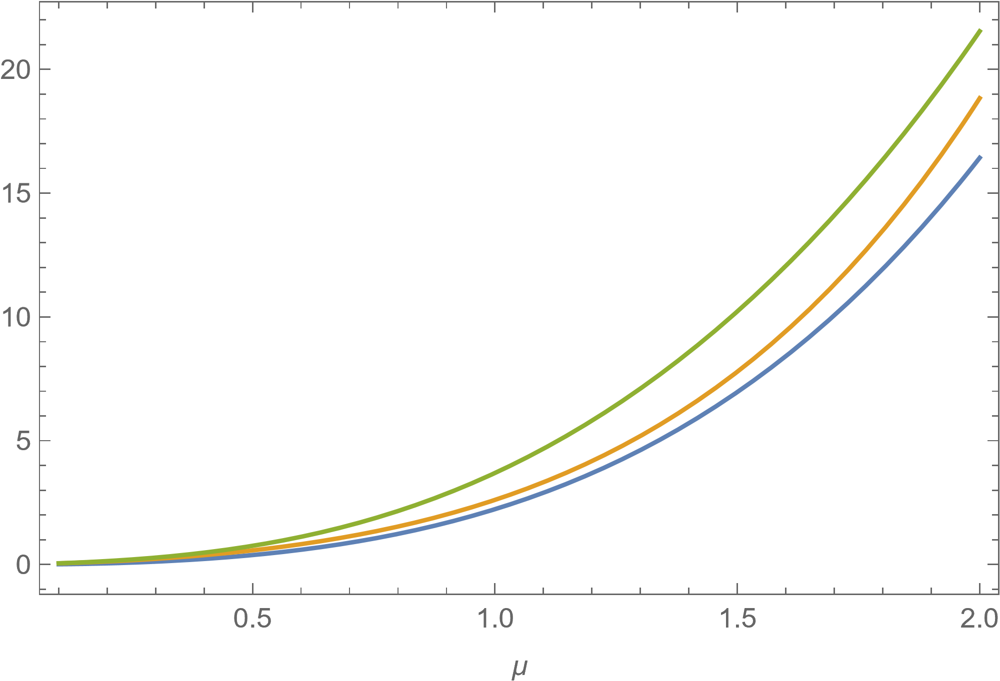
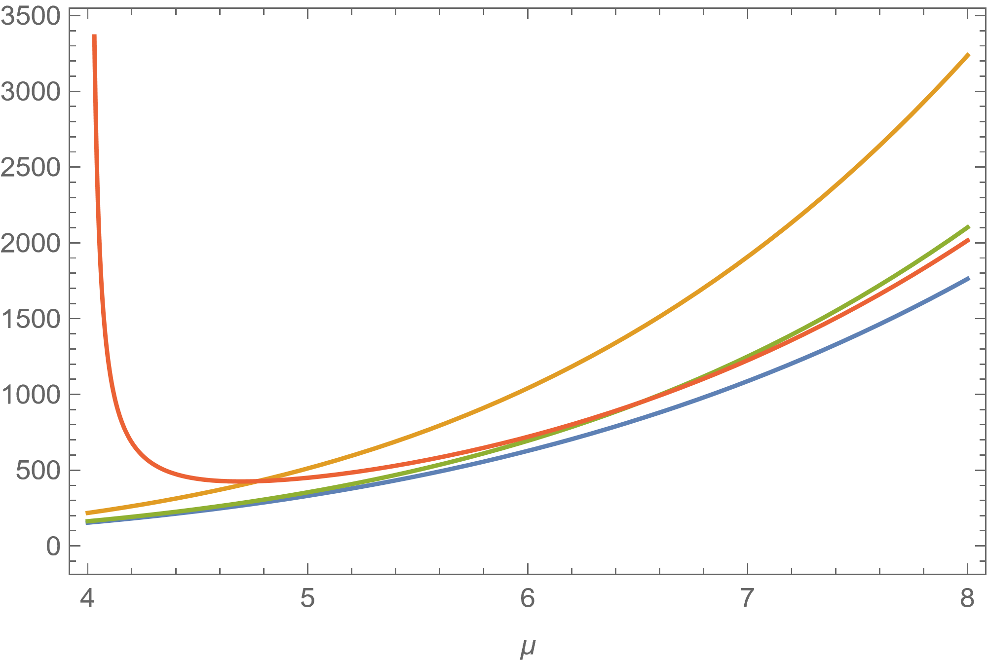
Figure 1: The images report the asymptotic variances of the MLE $\hat{\mu}_{n}^{\mathrm{ML}}$ , the moment estimator $\hat{\mu}_{n}^{\mathrm{MO}}$ (15) and the Stein estimator $\hat{\mu}_{n}^{\mathrm{ST}}$ (16) with tuning parameter $\kappa=10$ resp.  $\kappa=100$ .

3.4 Lomax distribution

The density of the Lomax distribution $LM(\alpha,\lambda)$ with $\theta=(\alpha,\lambda)$, $\alpha,\lambda>0$, is given by

$$p_{\theta}(x)=\frac{\alpha}{\lambda}\bigg{(}1+\frac{x}{\lambda}\bigg{)}^{-(\alpha+1)},\quad x>0.$$

We take $\tau_{\theta}(x)=x+\lambda$. Note that here $\mathbb{E}[X^{k}]$ for $X\sim LM(\alpha,\lambda)$ exists only if $k>\alpha$. Hence, a Stein operator is given by

$$\mathcal{A}_{\theta}f(x)=(x+\lambda)f^{\prime}(x)-\alpha f(x).$$

Our Stein estimators for test functions $f_{1}$, $f_{2}$ are given by

$$\hat{\alpha}_{n}= \frac{\overline{f_{2}^{\prime}(X)}\ \overline{Xf_{1}^{\prime}(X)}-\overline{f_{1}^{\prime}(X)}\ \overline{Xf_{2}^{\prime}(X)}}{\overline{f_{1}(X)}\ \overline{f_{2}^{\prime}(X)}-\overline{f_{1}^{\prime}(X)})\ \overline{f_{2}(X)}},$$

$$\hat{\lambda}_{n}= \frac{\overline{f_{2}(X)}\ \overline{Xf_{1}^{\prime}(X)}-\overline{f_{1}(X)}\ \overline{Xf_{2}^{\prime}(X)}}{\overline{f_{1}(X)}\ \overline{f_{2}^{\prime}(X)}-\overline{f_{1}^{\prime}(X)})\ \overline{f_{2}(X)}}.$$

The purpose of this section is to give an example of Theorem 2.16, that is an iterative procedure that generates a sequence of Stein estimators which converges to the MLE. Thereto, we examine the MLE, which we denote by $\hat{\theta}_{n}^{\mathrm{ML}}=(\hat{\alpha}_{n}^{\mathrm{ML}},\hat{\lambda}_{n}^{\mathrm{ML}})$, and is given through the equations

$$1=\bigg{(}1+\bigg{(}\frac{1}{n}\sum_{i=1}^{n}\log\big{(}1+X_{i}/\hat{\lambda}_{n}^{\mathrm{ML}}\big{)}\bigg{)}^{-1}\bigg{)}\bigg{(}\frac{1}{n}\sum_{i=1}^{n}\frac{X_{i}}{\hat{\lambda}_{n}^{\mathrm{ML}}+X_{i}}\bigg{)},$$ (17)

$$\hat{\alpha}_{n}^{\mathrm{ML}}=\bigg{(}\frac{1}{n}\sum_{i=1}^{n}\log\big{(}1+X_{i}/\hat{\lambda}_{n}^{\mathrm{ML}}\big{)}\bigg{)}^{-1}.$$ (18)

An explicit solution does not exit. We show in the next lemma that the MLE only exists under certain assumptions.

Lemma 3.1.

The MLE for the Lomax distribution $L(\alpha,\lambda)$ exists if and only if $\overline{X^{2}}-2\overline{X}^{2}>0.$

Proof.

In [28], it was shown that the likelihood function of the Lomax distribution with respect to an i.i.d. sample is strictly concave. Therefore, it admits at most one global maximum, and since the likelihood function is differentiable, this global maximum (if it exists) is characterized by (17) and (18). Since $\hat{\alpha}_{n}^{\mathrm{ML}}$ can be expressed explicitly as a function of $\hat{\lambda}_{n}^{\mathrm{ML}}$, it is clear that the MLE exists if and only if there is a $\hat{\lambda}_{n}^{\mathrm{ML}}$ that satisfies equation (17). In order to examine the latter question, we rearrange the equation and get

$$\frac{1}{n}\sum_{i=1}^{n}\log\big{(}1+X_{i}/\hat{\lambda}_{n}^{\mathrm{ML}}\big{)}=\bigg{(}\frac{1}{n}\sum_{i=1}^{n}\frac{X_{i}}{\hat{\lambda}_{n}^{\mathrm{ML}}+X_{i}}\bigg{)}\bigg{(}\frac{1}{n}\sum_{i=1}^{n}\log\big{(}1+X_{i}/\hat{\lambda}_{n}^{\mathrm{ML}}\big{)}+1\bigg{)}.$$ (19)

We define

$$\ell_{1}(\gamma)=\frac{1}{n}\sum_{i=1}^{n}\log\big{(}1+\gamma X_{i}\big{)}\quad\text{and}\quad\ell_{2}(\gamma)=\bigg{(}\frac{1}{n}\sum_{i=1}^{n}\frac{\gamma X_{i}}{1+\gamma X_{i}}\bigg{)}\bigg{(}\frac{1}{n}\sum_{i=1}^{n}\log\big{(}1+\gamma X_{i}\big{)}+1\bigg{)},$$

and can rewrite (19) by $\ell_{1}(1/\hat{\lambda}_{n}^{\mathrm{ML}})=\ell_{2}(1/\hat{\lambda}_{n}^{\mathrm{ML}})$. It is clear that for $\gamma>0$ large enough we will eventually have $\ell_{2}(\gamma)>\ell_{1}(\gamma)$. Moreover, it is an easy task to compute the limits $\lim_{\gamma\rightarrow 0}\ell_{1,2}(\gamma)=0$ and $\lim_{\gamma\rightarrow\infty}\ell_{1,2}(\gamma)=\infty$. Furthermore, $\lim_{\gamma\rightarrow 0}\ell_{1,2}^{\prime}(\gamma)=\overline{X}$. With the concavity of the likelihood function, it is clear that $\ell_{1}$ and $\ell_{2}$ intersect at most once for $\gamma>0$. By considering the aforementioned limits, this is the case if and only if $\lim_{\gamma\rightarrow 0}\ell_{1}^{\prime\prime}(\gamma)>\lim_{\gamma\rightarrow 0}\ell_{2}^{\prime\prime}(\gamma)$. Tedious calculations yield $\lim_{\gamma\rightarrow 0}\ell_{1}^{\prime\prime}(\gamma)=-\overline{X^{2}}$ and $\lim_{\gamma\rightarrow 0}\ell_{2}^{\prime\prime}(\gamma)=-2\overline{X^{2}}+2\overline{X}^{2}$, which concludes the proof. ∎

In [28], the authors also report difficulties when performing MLE, which is in accordance with Lemma 3.1. It is interesting to see that the MLE exists if and only if the moment estimator $\hat{\lambda}_{n}^{\mathrm{MO}}$ is positive. We now show that the condition for the existence of the MLE above is asymtotically satisfied and therefore complies with Assumption 2.15(a).

Lemma 3.2.

If $X_{1},\ldots,X_{n}\sim L(\alpha,\lambda)$, then $\overline{X^{2}}-2\overline{X}^{2}>0$ with probability converging to one.

Proof.

Note that the event $\{\omega\in\Omega\,|\,\overline{X^{2}}-2\overline{X}^{2}>0\}$ is independent of $\lambda>0$, and we can therefore assume without loss of generality that $\lambda=1$. We first treat the case $\alpha>2$. In this case,

$$\mathbb{P}(\overline{X^{2}}-2\overline{X}^{2}>0) =\mathbb{P}\Big{(}\overline{X^{2}}-2\overline{X}^{2}-\big{(}\mathbb{E}[X^{2}]-2\mathbb{E}[X]^{2}\big{)}>-\big{(}\mathbb{E}[X^{2}]-2\mathbb{E}[X]^{2}\big{)}\Big{)}$$

$$=\mathbb{P}\Big{(}\mathbb{E}[X^{2}]-2\mathbb{E}[X]^{2}-\big{(}\overline{X^{2}}-2\overline{X}^{2}\big{)}<\mathbb{E}[X^{2}]-2\mathbb{E}[X]^{2}\Big{)}$$

$$\geq\mathbb{P}\bigg{(}\big{|}\mathbb{E}[X^{2}]-2\mathbb{E}[X]^{2}-\big{(}\overline{X^{2}}-2\overline{X}^{2}\big{)}\big{|}<\frac{2}{(\alpha-1)^{2}(\alpha-2)}\bigg{)},$$

where $X\sim L(\alpha,1)$. The last expression converges to $1$ due to the strong law of large numbers. Let now $0<\alpha<2$, and let $\tilde{X}_{1},\ldots\tilde{X}_{n}\sim L(\tilde{\alpha},1)$ be i.i.d. with $\tilde{\alpha}>2$. By examining the cdf of the Lomax distribution, one realises that $X_{i}$ and $\tilde{X}_{i}$ are stochastically ordered $X_{i}\prec\tilde{X}_{i}$ for each $i=1,\ldots,n$ with respect to the standard ordering

$$X\prec Y\quad\text{if and only if}\quad\mathbb{P}(X>x)\leq\mathbb{P}(Y>x)$$

for all $x\in\mathbb{R}$, where $X$ and $Y$ are two real-valued random variables. We define the function

$$F:\mathbb{R}_{+}^{n}\rightarrow\mathbb{R},\>x\mapsto\frac{1}{n}\sum_{i=1}^{n}x_{i}^{2}-2\bigg{(}\frac{1}{n}\sum_{i=1}^{n}x_{i}\bigg{)}^{2},$$

and have

$$\frac{\partial}{\partial x_{j}}F(x)=\frac{2x_{j}}{n}\bigg{(}1-2\frac{1}{n}\sum_{i=1}^{n}x_{i}\bigg{)}.$$

It is clear that for each $x\in\mathbb{R}_{+}^{n}$ that satisfies $1-2\frac{1}{n}\sum_{i=1}^{n}x_{i}<0$, the function $F$ is monotonically decreasing in each component. We now define the sequence of sets $A_{n}$, $n\in\mathbb{N}$ by $A_{n}=\{\omega\in\Omega\,|\,1-2\overline{X}<0\}$. Then we know that for the conditional distributions we get

$$\frac{1}{n}\sum_{i=1}^{n}X_{i}^{2}-2\bigg{(}\frac{1}{n}\sum_{i=1}^{n}X_{i}\bigg{)}^{2}\,\bigg{|}\,A_{n}\succ\frac{1}{n}\sum_{i=1}^{n}\tilde{X}_{i}^{2}-2\bigg{(}\frac{1}{n}\sum_{i=1}^{n}\tilde{X}_{i}\bigg{)}^{2}\,\bigg{|}\,A_{n}.$$

With the strong law of large numbers, $1-2\overline{X}$ will converge almost surely to $\frac{\alpha-2}{\alpha-1}<0$ if $1<\alpha<2$ and will diverge to $-\infty$ if $0<\alpha<1$, as $n\rightarrow\infty$. Hence, we conclude that $\mathbb{P}(A_{n})\rightarrow 1$. Now, let $B_{n}=\{\omega\in\Omega\,|\,\overline{X^{2}}-2\overline{X}^{2}>0\}$. Then

$$\mathbb{P}(B_{n}) =\mathbb{P}(B_{n}\,|\,A_{n})\mathbb{P}(A_{n})+\mathbb{P}(B_{n}\,|\,\bar{A}_{n})\mathbb{P}(\bar{A}_{n})$$

$$\geq\mathbb{P}\bigg{(}\frac{1}{n}\sum_{i=1}^{n}\tilde{X}_{i}^{2}-2\bigg{(}\frac{1}{n}\sum_{i=1}^{n}\tilde{X}_{i}\bigg{)}^{2}>0\,\bigg{|}\,A_{n}\bigg{)}\mathbb{P}(A_{n})+\mathbb{P}(B_{n}\,|\,\bar{A}_{n})\mathbb{P}(\bar{A}_{n}),$$

which converges to $1$ by the first part of the proof. ∎

We profit from the simplicity of the cdf, which is given by

$$P_{\theta}(x)=1-\bigg{(}1+\frac{x}{\lambda}\bigg{)}^{-\alpha},\quad x>0.$$

The optimal functions are therefore

$$f_{\theta}^{(1)}(x)=\frac{\log\big{(}1+\frac{x}{\lambda}\big{)}}{\alpha}\quad\text{and}\quad f_{\theta}^{(2)}(x)=-\frac{x}{\lambda(x+\lambda)}.$$

It remains to verify Assumptions 2.15(c), (b) and (d), of which the latter two can be easily checked. We have a closer look at (c), more precisely at the condition that $\mathbb{E}[M_{\theta}(X)]\frac{\partial}{\partial\theta}g(\theta)$ needs to be invertible on $\Theta_{0}$. We compute

$$M_{\theta}(x)\frac{\partial}{\partial\theta}g(\theta)=\begin{pmatrix}-f_{\theta}^{(1)}(x)&\big{(}f_{\theta}^{(1)}\big{)}^{\prime}(x)\\ -f_{\theta}^{(2)}(x)&\big{(}f_{\theta}^{(2)}\big{)}^{\prime}(x)\end{pmatrix}.$$

We have to show that the expectation with respect to $\mathbb{P}_{\theta_{0}}$ of the latter matrix is invertible for all $(\alpha_{0},\lambda_{0})\in\Theta$ and $(\alpha,\lambda)\in\Theta_{0}$. We show that the determinant

$$\det\bigg{(}\mathbb{E}\bigg{[}M_{\theta}(X)\frac{\partial}{\partial\theta}g(\theta)\bigg{]}\bigg{)}=\mathbb{E}\big{[}\big{(}f_{\theta}^{(1)}\big{)}^{\prime}(X)\big{]}\mathbb{E}\big{[}f_{\theta}^{(2)}(X)\big{]}-\mathbb{E}\big{[}\big{(}f_{\theta}^{(2)}\big{)}^{\prime}(X)\big{]}\mathbb{E}\big{[}f_{\theta}^{(1)}(X)\big{]},$$ (20)

where $X\sim\mathbb{P}_{\theta_{0}}$, is always positive. Note first that the derivatives of our optimal functions are given by

$$\big{(}f_{\theta}^{(1)}\big{)}^{\prime}(x)=\frac{1}{\alpha}\frac{1}{x+\lambda}\quad\text{and}\quad\big{(}f_{\theta}^{(2)}\big{)}^{\prime}(x)=-\frac{1}{(x+\lambda)^{2}}.$$

Then by applying dominated and monotone convergence to each expectation in (20), we obtain that the determinant diverges to $\infty$ as $\lambda\rightarrow 0$ and converges to $0$ as $\lambda\rightarrow\infty$. After examining the signs of each expectation, we conclude that the determinant is monotonically decreasing in $\lambda$. Moreover, the sign of the determinant is independent of $\alpha$, since we have dependence only through $f_{\theta}^{(1)}$, $\big{(}f_{\theta}^{(1)}\big{)}^{\prime}$ and $\alpha>0$. The latter reasoning is true for all $(\alpha_{0},\lambda_{0})\in\Theta$, and thus Assumption 2.15(c) is verified. In summary, we can apply Theorem 2.16 and state that the iteratively defined sequence of Stein estimators is converging to the MLE with probability converging to $1$ as the sample size grows. For the sake of completeness, we also give the asymptotic variance of the MLE, which is the inverse of the Fisher information matrix and given by

$$I_{\mathrm{ML}}^{-1}(\alpha,\lambda)=(\alpha+1)\begin{pmatrix}(\alpha+1)\alpha^{2}&\lambda(\alpha+2)\alpha\\ \lambda(\alpha+2)\alpha&\frac{\lambda^{2}(\alpha+1)(\alpha+2)}{\alpha}\end{pmatrix}.$$

Since there is an interesting link between the existence of the MLE and the moment estimator, we shortly consider the latter. The classical moment estimator (which is only consistent if $\alpha>2$) is obtained through the functions $f_{1}(x)=x$ and $f_{2}(x)=x^{2}$, which gives

$$\hat{\alpha}_{n}^{\mathrm{MO}}=\frac{2\overline{X}^{2}-2\overline{X^{2}}}{2\overline{X}^{2}-\overline{X^{2}}}\quad\text{and}\quad\hat{\lambda}_{n}^{\mathrm{MO}}=\frac{\overline{X}\,\overline{X^{2}}}{\overline{X^{2}}-2\overline{X}^{2}}.$$

Now it can be seen directly from Lemma 3.1 that the MLE exists if and only if $\hat{\lambda}_{n}^{\mathrm{MO}}$ is positive. The asymptotic variance of $\hat{\theta}_{n}^{\mathrm{MO}}$ can be computed explicitly and is given by

$$\frac{\alpha(\alpha-1)^{2}}{(\alpha-3)(\alpha-4)}\begin{pmatrix}(\alpha-2)(6+(\alpha-1)\alpha)&\lambda(4+(\alpha-2)\alpha)\\ \lambda(4+(\alpha-2)\alpha)&\frac{\lambda^{2}(4+(\alpha-3)\alpha)}{\alpha-2}\end{pmatrix}.$$

Note that the latter formula is only valid for $\alpha>4$. A further discussion on fitting the Lomax distribution is available in [45], although the authors perform simulation studies with contaminated data.

3.5 Nakagami distribution

The density of the Nakagami distribution $NG(m,\Omega)$ with $\theta=(m,\Omega)$, $m,\Omega>0$, is given by

$$p_{\theta}(x)=\frac{2m^{m}}{\Gamma(m)\Omega^{m}}x^{2m-1}\exp\bigg{(}-\frac{m}{\Omega}x^{2}\bigg{)},\quad x>0.$$

We take $\tau_{\theta}(x)=\Omega x$. A Stein operator is given by

$$\mathcal{A}_{\theta}f(x)=2m(\Omega-x^{2})f(x)+x\Omega f^{\prime}(x)$$

(see [25]). The Stein estimators for test functions $f_{1}$, $f_{2}$ are given by

$$\hat{m}_{n}= \frac{1}{2}\frac{\overline{X^{2}f_{2}(X)}\ \overline{Xf_{1}^{\prime}(X)}-\overline{X^{2}f_{1}(X)}\ \overline{Xf_{2}^{\prime}(X)}}{\overline{f_{2}(X)}\ \overline{X^{2}f_{1}(X)}-\overline{f_{1}(X)}\ \overline{X^{2}f_{2}(X)}},$$

$$\hat{\Omega}_{n}= \frac{\overline{X^{2}f_{2}(X)}\ \overline{Xf_{1}^{\prime}(X)}-\overline{X^{2}f_{1}(X)}\ \overline{Xf_{2}^{\prime}(X)}}{\overline{f_{2}(X)}\ \overline{Xf_{1}^{\prime}(X)}-\overline{f_{1}(X)})\ \overline{Xf_{2}^{\prime}(X)}}.$$

As to other estimation methods, we consider the standard moment estimator, which we denote by $\hat{\theta}_{n}^{\mathrm{MO1}}=(\hat{m}_{n}^{\mathrm{MO1}},\hat{\Omega}_{n}^{\mathrm{MO1}})$, and give the first two moments

$$\begin{split}\mathbb{E}[X]=\frac{\Gamma(m+\frac{1}{2})}{\Gamma(m)}\bigg{(}\frac{\Omega}{m}\bigg{)}^{1/2}\quad\text{and}\quad\mathbb{E}[X^{2}]=\Omega.\end{split}$$ (21)

As can be easily seen from (21), $\hat{m}_{n}^{\mathrm{MO1}}$ is not explicit and requires a numerical procedure in order to solve the non-linear equation. Note that we are not able to retrieve these estimators with specific test functions. This can be readily seen since our estimators are always explicit, regardless of the choice of test functions. However, the asymptotic variance of the moment estimator can be calculated explicitly and is given by the matrix $V_{\mathrm{MO1}}(\theta)$ with entries

$$\big{(}V_{\mathrm{MO1}}(\theta)\big{)}_{11}=\frac{m\big{(}4m^{2}+(m+1)((m)_{\nicefrac{{1}}{{2}}}){}^{2}-4(m)_{\nicefrac{{1}}{{2}}}(m)_{\nicefrac{{3}}{{2}}}\big{)}}{((m)_{\nicefrac{{1}}{{2}}}){}^{2}\big{(}2m\psi(m)-2m\psi(m+\frac{1}{2})+1\big{)}^{2}},\qquad\big{(}V_{\mathrm{MO1}}(\theta)\big{)}_{22}=\frac{(m+1)\Omega^{2}}{m},$$

$$\big{(}V_{\mathrm{MO1}}(\theta)\big{)}_{12}=\big{(}V_{\mathrm{MO1}}(\theta)\big{)}_{21}=\frac{m\Omega}{-2m\psi(m)+2m\psi(m+\frac{1}{2})-1},$$

where $(a)_{b}=\frac{\Gamma(a+1)}{\Gamma(a-b+1)}$ denotes the Pochhammer symbol. In [3], the moment estimators

$$\begin{split}\hat{m}_{n}^{\mathrm{MO2}}=\frac{\overline{X^{2}}}{\overline{X^{4}}-\overline{X^{2}}}\quad\text{and}\quad\hat{\Omega}_{n}^{\mathrm{MO2}}=\overline{X^{2}}\end{split}$$ (22)

are proposed (which are obtained through the test functions $f_{1}(x)=1$, $f_{2}(x)=x^{2}$ in our approach). However, the authors do not calculate the asymptotic variance, which is easily computed through Theorem 2.5, and is given by

$$V_{\mathrm{MO2}}(\theta)=\begin{pmatrix}2m(m+1)&0\\ 0&\frac{\Omega^{2}}{m}\end{pmatrix}.$$

The MLE $\hat{\theta}_{n}^{\mathrm{ML}}=(\hat{m}_{n}^{\mathrm{ML}},\hat{\Omega}_{n}^{\mathrm{ML}})$ is described by

$$\begin{split}\log\hat{m}_{n}^{\mathrm{ML}}-\psi(\hat{m}_{n}^{\mathrm{ML}})&=\log\overline{X^{2}}-2\overline{\log X},\\ \hat{\Omega}_{n}^{\mathrm{ML}}&=\overline{X^{2}},\end{split}$$ (23)

and is uniquely determined by (23) and exists almost surely. To see that, note that the likelihood function admits exactly one critical point at $(\hat{m}_{n}^{\mathrm{ML}},\hat{\Omega}_{n}^{\mathrm{ML}})$, which can be identified to be a local maximum by the second derivative test. Although the likelihood is not necessarily concave, we know that for each $m>0$ the function $\Omega\mapsto\sum_{i=1}^{n}\log p_{\theta}(X_{i})$ has a global maximum at $\Omega=\hat{\Omega}_{n}^{\mathrm{ML}}$ and the function $m\mapsto\sum_{i=1}^{n}\log p_{(m,\hat{\Omega}_{n}^{\mathrm{ML}})}(X_{i})$ has a global maximum at $m=\hat{m}_{n}^{\mathrm{ML}}$, which yields that the local maximum of the likelihood function is also a global one. In [42], multiple algorithms for solving the likelihood equation are compared, which boils down to a comparison of approximations of the digamma function. Since we deal with a regular probability distribution, we know that the asymptotic covariance matrix of the MLE is given by the inverse of the Fisher information matrix, which is equal to

$$I_{\mathrm{ML}}^{-1}(\theta)=\begin{pmatrix}\frac{m}{m\psi(m)-1}&0\\ 0&\frac{\Omega^{2}}{m}\end{pmatrix}.$$

Regarding the Stein estimator, we propose to use the natural test functions $f_{1}(x)=1$ and $f_{2}(x)=x$, which yield the new estimators

$$\hat{m}_{n}^{\mathrm{ST1}}=\frac{1}{2}\frac{\overline{X^{2}}\ \overline{X}}{\overline{X^{3}}-\overline{X}\ \overline{X^{2}}}\quad\text{and}\quad\hat{\Omega}_{n}^{\mathrm{ST1}}=\overline{X^{2}}.$$ (24)

An application of a multivariate version of Jensen’s inequality yields that both estimates in (24) are always positive, whereas the (modified) moment estimators (22) may not exist for small sample sizes. With Theorem 2.5, we compute the asymptotic variance of the Stein estimator, and obtain $V_{\mathrm{ST1}}$ with entries

$$\big{(}V_{\mathrm{ST1}}(\theta)\big{)}_{11}=\frac{m(5+4m)\Gamma(1+m)^{2}}{\Gamma(\nicefrac{{1}}{{2}}+m)^{2}}-m(1+2m)^{2},\quad\big{(}V_{\mathrm{ST1}}(\theta)\big{)}_{12}=\big{(}V_{\mathrm{ST1}}(\theta)\big{)}_{21}=0,\quad\big{(}V_{\mathrm{ST1}}(\theta)\big{)}_{22}=\frac{\Omega^{2}}{m}.$$

Lastly, we consider the two-step Stein estimator, which we denote by $\hat{\theta}_{n}^{\mathrm{ST2}}=(\hat{m}_{n}^{\mathrm{ST2}},\hat{\Omega}_{n}^{\mathrm{ST2}})$. The optimal functions are given by

$$f_{\theta}^{(1)}(x) =\frac{1}{2m^{3}x^{2m}}\bigg{(}\frac{\Omega}{m}\bigg{)}^{m-1}\bigg{(}\bigg{(}\frac{mx^{2}}{\Omega}\bigg{)}^{m}\bigg{(}m-\exp\bigg{(}\frac{mx^{2}}{\Omega}\bigg{)}\,_{2}F_{2}\bigg{(}m,m;m+1,m+1;-\frac{mx^{2}}{\Omega}\bigg{)}\bigg{)}$$

$$\quad+m^{2}\exp\bigg{(}\frac{mx^{2}}{\Omega}\bigg{)}\gamma\bigg{(}m,\frac{mx^{2}}{\Omega}\bigg{)}\bigg{(}\log\bigg{(}\frac{mx^{2}}{\Omega}\bigg{)}-\psi(m)\bigg{)}\bigg{)},$$

$$f_{\theta}^{(2)}(x) =-\frac{1}{2\Omega^{2}}.$$

Once again the derivatives can be expressed in terms of the original functions. We obtain

$$\big{(}f_{\theta}^{(1)}\big{)}^{\prime}(x)=\frac{1-\frac{x^{2}}{\Omega}+\log\big{(}\frac{mx^{2}}{\Omega}\big{)}-\psi(m)}{\Omega x}-m\bigg{(}\frac{2}{x}-\frac{2x}{\Omega}\bigg{)}f_{\theta}^{(1)}(x).$$

Analogous to the gamma example of Section 3.1, the necessary assumptions for Theorems 2.11 and 2.12 can be verified and the latter two theorems are applicable for a suitable first-step estimator, which we choose to be the explicit Stein estimator $\hat{\theta}_{n}^{\mathrm{ST1}}$. By studying the corresponding asymptotic covariance matrix, it is evident that the moment estimators (21) perform poorly, which is why we excluded the latter below. In Figure 2, the asymptotic variances of the (modified) moment estimator, the MLE and the Stein estimator $\hat{m}_{n}^{\mathrm{ST1}}$ of $m$ are plotted for a range of values of $m_{0}$. Note that estimators for $\Omega$ coincide for all considered estimation methods. We observe that we improve on the (modified) moment estimator in terms of asymptotic variance but do not reach efficiency. To our knowledge, $\hat{m}_{n}^{\mathrm{ST1}}$ is the best (in terms of asymptotic variance) explicit estimator available for the parameter $m$ of the Nakagami distribution. This, motivates using the estimates of the explicit Stein estimator as starting values for other procedures, for example the MLE. We also performed a simulation study, whose results are reported in Tables 5 and 6. Here we also included the asymptotically efficient two-step Stein estimator $\hat{\theta}_{n}^{\mathrm{ST2}}$ (with first-step estimator $\hat{\theta}_{n}^{\mathrm{ST1}}$). The (modified) moment estimator served as an initial guess for the MLE. We notice that the MLE seems to be globally the best, followed by the two-step Stein estimator and the explicit Stein estimator. The (modified) moment estimator is clearly outperformed for most parameter constellations in terms of bias and MSE. We find that the estimator $\hat{m}_{n}^{\mathrm{ST2}}$ seems to break down completely for $(m_{0},\Omega_{0})=(2,5)$. Furthermore, we found the function $f_{\theta}^{(1)}$ to be numerically hard to evaluate when $m_{0}<1/2$, which is why we excluded the latter case from the simulation study.

$\theta_{0}$		Bias				MSE
		$\hat{\theta}_{n}^{\mathrm{MO2}}$	$\hat{\theta}_{n}^{\mathrm{ML}}$	$\hat{\theta}_{n}^{\mathrm{ST1}}$	$\hat{\theta}_{n}^{\mathrm{ST2}}$	$\hat{\theta}_{n}^{\mathrm{MO2}}$	$\hat{\theta}_{n}^{\mathrm{ML}}$	$\hat{\theta}_{n}^{\mathrm{ST1}}$	$\hat{\theta}_{n}^{\mathrm{ST2}}$
$(1,1)$	$m$	2.23	0.146	0.198	0.191	$1.29\text{e4}$	0.162	0.226	0.191
	$\Omega$	$-2.83\text{e-3}$	$-2.83\text{e-3}$	$-2.83\text{e-3}$	$-2.83\text{e-3}$	0.052	0.052	0.052	0.052
$(0.8,1)$	$m$	0.805	0.108	0.164	0.152	444	0.092	0.143	0.129
	$\Omega$	$-2.12\text{e-3}$	$-2.12\text{e-3}$	$-2.12\text{e-3}$	$-2.12\text{e-3}$	0.063	0.063	0.063	0.063
$(1.4,0.8)$	$m$	0.17	0.21	0.266	0.258	$1.8\text{e4}$	0.336	0.428	0.383
	$\Omega$	$-2.75\text{e-3}$	$-2.75\text{e-3}$	$-2.75\text{e-3}$	$-2.75\text{e-3}$	0.023	0.023	0.023	0.023
$(3,5)$	$m$	$-2.81$	0.495	0.544	0.587	7.92	1.75	1.95	2.43
	$\Omega$	$-7.09\text{e-3}$	$-7.09\text{e-3}$	$-7.09\text{e-3}$	$-8.88\text{e-3}$	0.415	0.415	0.415	0.413
$(3,1)$	$m$	1.7	0.48	0.531	0.528	6781	1.7	1.89	1.85
	$\Omega$	$-9.02\text{e-4}$	$-9.02\text{e-4}$	$-9.02\text{e-4}$	$-9.02\text{e-4}$	0.017	0.017	0.017	0.017
$(2,5)$	$m$	$-1.83$	0.32	0.379	0.975	3.36	0.72	0.864	1277
	$\Omega$	$-1.56\text{e-3}$	$-1.56\text{e-3}$	$-1.56\text{e-3}$	-0.017	0.605	0.605	0.605	0.596
$(4,0.5)$	$m$	$-6.76$	0.682	0.74	0.736	47.6	3.18	3.45	3.41
	$\Omega$	$-1.22\text{e-4}$	$-1.22\text{e-4}$	$-1.22\text{e-4}$	$-1.22\text{e-4}$	$3.17\text{e-3}$	$3.17\text{e-3}$	$3.17\text{e-3}$	$3.17\text{e-3}$
$(8,4)$	$m$	$-7.71$	1.37	1.41	1.41	59.4	13.3	13.7	13.6
	$\Omega$	$2.3\text{e-4}$	$2.31\text{e-4}$	$2.3\text{e-4}$	$2.3\text{e-4}$	0.1	0.1	0.1	0.1
$(3,3)$	$m$	$-2.64$	0.486	0.535	0.537	7	1.72	1.91	1.86
	$\Omega$	$-4.62\text{e-3}$	$-4.62\text{e-3}$	$-4.62\text{e-3}$	$-4.62\text{e-3}$	0.149	0.149	0.149	0.149
$(0.8,0.2)$	$m$	$-2.46$	0.109	0.158	0.143	507	0.092	0.14	0.11
	$\Omega$	$-6.05\text{e-4}$	$-6.05\text{e-4}$	$-6.05\text{e-4}$	$-6.05\text{e-4}$	$2.52\text{e-3}$	$2.52\text{e-3}$	$2.52\text{e-3}$	$2.52\text{e-3}$

Table 5: Simulation results for the $N(m,\Omega)$ distribution for $n=20$ and $10,000$ repetitions.

$\theta_{0}$		Bias				MSE
		$\hat{\theta}_{n}^{\mathrm{MO2}}$	$\hat{\theta}_{n}^{\mathrm{ML}}$	$\hat{\theta}_{n}^{\mathrm{ST1}}$	$\hat{\theta}_{n}^{\mathrm{ST2}}$	$\hat{\theta}_{n}^{\mathrm{MO2}}$	$\hat{\theta}_{n}^{\mathrm{ML}}$	$\hat{\theta}_{n}^{\mathrm{ST1}}$	$\hat{\theta}_{n}^{\mathrm{ST2}}$
$(1,1)$	$m$	0.32	0.053	0.077	0.074	40.2	0.042	0.063	0.047
	$\Omega$	$2.95\text{e-3}$	$2.95\text{e-3}$	$2.95\text{e-3}$	$2.95\text{e-3}$	0.02	0.02	0.02	0.02
$(0.8,1)$	$m$	0.193	0.037	0.06	0.056	2.64	0.024	0.04	0.03
	$\Omega$	$-1.74\text{e-3}$	$-1.74\text{e-3}$	$-1.74\text{e-3}$	$-1.74\text{e-3}$	0.025	0.025	0.025	0.025
$(1.4,0.8)$	$m$	5.34	0.078	0.101	0.099	$6.71\text{e4}$	0.086	0.115	0.095
	$\Omega$	$-5.51\text{e-4}$	$-5.52\text{e-4}$	$-5.51\text{e-4}$	$-5.51\text{e-4}$	$9.26\text{e-3}$	$9.26\text{e-3}$	$9.26\text{e-3}$	$9.26\text{e-3}$
$(3,5)$	$m$	$-2.82$	0.195	0.216	0.223	7.95	0.451	0.517	0.481
	$\Omega$	$4.23\text{e-3}$	$4.22\text{e-3}$	$4.23\text{e-3}$	$4.23\text{e-3}$	0.165	0.165	0.165	0.165
$(3,1)$	$m$	1.47	0.176	0.2	0.199	874	0.436	0.509	0.485
	$\Omega$	$-3.93\text{e-4}$	$-3.93\text{e-4}$	$-3.93\text{e-4}$	$-3.93\text{e-4}$	$6.66\text{e-3}$	$6.66\text{e-3}$	$6.66\text{e-3}$	$6.66\text{e-3}$
$(2,5)$	$m$	$-1.84$	0.113	0.135	0.213	3.39	0.185	0.227	3.41
	$\Omega$	$-1.35\text{e-4}$	$-1.32\text{e-4}$	$-1.35\text{e-4}$	$-1.67\text{e-3}$	0.246	0.246	0.246	0.246
$(4,0.5)$	$m$	$-6.7$	0.235	0.256	0.256	45.1	0.783	0.874	0.853
	$\Omega$	$5.52\text{e-4}$	$5.51\text{e-4}$	$5.52\text{e-4}$	$5.52\text{e-4}$	$1.23\text{e-3}$	$1.23\text{e-3}$	$1.23\text{e-3}$	$1.23\text{e-3}$
$(8,4)$	$m$	$-7.71$	0.49	0.505	0.506	59.5	3.33	3.48	3.45
	$\Omega$	$2.73\text{e-3}$	$2.73\text{e-3}$	$2.73\text{e-3}$	$2.73\text{e-3}$	0.041	0.041	0.041	0.041
$(3,3)$	$m$	$-2.66$	0.19	0.215	0.215	7.06	0.45	0.52	0.491
	$\Omega$	$-1.86\text{e-3}$	$-1.86\text{e-3}$	$-1.86\text{e-3}$	$-1.86\text{e-3}$	0.061	0.061	0.061	0.061
$(0.8,0.2)$	$m$	$-2.66$	0.042	0.067	0.058	10.9	0.026	0.042	0.029
	$\Omega$	$3.11\text{e-4}$	$3.11\text{e-4}$	$3.11\text{e-4}$	$3.11\text{e-4}$	$1\text{e-3}$	$1\text{e-3}$	$1\text{e-3}$	$1\text{e-3}$

Table 6: Simulation results for the $N(m,\Omega)$ distribution for $n=50$ and $10,000$ repetitions.

Figure 2: Asymptotic variances of the estimators of the parameter $m$ of the Nakagami distribution. Plotted are the MLE $\hat{m}_{n}^{\mathrm{ML}}$ , the moment estimator $\hat{m}_{n}^{\mathrm{MO}}$ (22) and the Stein estimator $\hat{m}_{n}^{\mathrm{ST}}$ (24). Note the value is independent of $\Omega$

3.6 Truncated Normal distribution

The density of the two-sided truncated Gaussian distribution on $(a,b)$ with $a,b\in\mathbb{R}$, denoted by $TN(\mu,\sigma^{2})$, $\theta=(\mu,\sigma^{2})$, is given by

$$p_{\theta}(x)=\frac{1}{\sigma}\frac{\phi\big{(}\frac{x-\mu}{\sigma}\big{)}}{\Phi\big{(}\frac{b-\mu}{\sigma}\big{)}-\Phi\big{(}\frac{a-\mu}{\sigma}\big{)}},$$

where $\phi$ and $\Phi$ are the standard Gaussian pdf and cdf. With $\tau_{\theta}(x)=\sigma^{2}$ we obtain the same Stein operator as in Example 1.2,

$$\mathcal{A}_{\theta}f(x)=\sigma^{2}f^{\prime}(x)+(\mu-x)f(x).$$

Note that the function class $\mathscr{F}_{\theta}$ differs from the one in the untruncated case. As we have the same Stein operator as in Example 1.2, we obtain for two different test functions $f_{1}$, $f_{2}$ the same expressions for our new estimators

$$\hat{\mu}_{n}= \frac{\overline{f_{2}^{\prime}(X)}\ \overline{Xf_{1}(X)}-\overline{f_{1}^{\prime}(X)}\ \overline{Xf_{2}(X)}}{\overline{f_{1}(X)}\ \overline{f_{2}^{\prime}(X)}-\overline{f_{1}^{\prime}(X)})\ \overline{f_{2}(X)}},$$

$$\hat{\sigma}_{n}^{2}= \frac{\overline{f_{1}(X)}\ \overline{Xf_{2}(X)}-\overline{f_{2}(X)}\ \overline{Xf_{1}(X)}}{\overline{f_{1}(X)}\ \overline{f_{2}^{\prime}(X)}-\overline{f_{1}^{\prime}(X)})\ \overline{f_{2}(X)}}.$$

Note that the complicated normalizing constant drops out and therefore completely explicit and easily computable estimators are retrieved. A natural choice seems to be the polynomials

$$f_{1}(x)= -x^{2}+(a+b)x-ab,$$

$$f_{2}(x)= x^{3}-\frac{3}{2}(a+b)x^{2}-\frac{1}{2}(-a^{2}-4ab-b^{2})x-\frac{1}{2}(a^{2}b+ab^{2}).$$

The Stein estimator based on the latter test functions will be denoted by $\hat{\theta}_{n}^{\mathrm{ST}}=(\hat{\mu}_{n}^{\mathrm{ST}},\hat{\sigma}_{n}^{\mathrm{ST}})$. It can be shown in a similar manner to the previous sections that Assumptions 2.2(a)–(b) are satisfied. However, we would like to compare their performance with that of the classical moment estimators $\hat{\mu}_{n}^{\mathrm{MO}}$ and $\hat{\sigma}_{n}^{\mathrm{MO}}$ based on the expectations

$$\mathbb{E}[X] =\mu-\sigma\frac{\phi\big{(}\frac{b-\mu}{\sigma}\big{)}-\phi\big{(}\frac{a-\mu}{\sigma}\big{)}}{\Phi\big{(}\frac{b-\mu}{\sigma}\big{)}-\Phi\big{(}\frac{a-\mu}{\sigma}\big{)}},$$

$$\mathbb{E}[X^{2}] =\mu^{2}+\sigma^{2}\bigg{(}1-\frac{\frac{b-\mu}{\sigma}\phi\big{(}\frac{b-\mu}{\sigma}\big{)}-\frac{a-\mu}{\sigma}\phi\big{(}\frac{a-\mu}{\sigma}\big{)}}{\Phi\big{(}\frac{b-\mu}{\sigma}\big{)}-\Phi\big{(}\frac{a-\mu}{\sigma}\big{)}}\bigg{)}-2\mu\sigma\frac{\phi\big{(}\frac{b-\mu}{\sigma}\big{)}-\phi\big{(}\frac{a-\mu}{\sigma}\big{)}}{\Phi\big{(}\frac{b-\mu}{\sigma}\big{)}-\Phi\big{(}\frac{a-\mu}{\sigma}\big{)}},$$

where $X\sim TN(\mu,\sigma^{2})$. We also include the MLE $\hat{\theta}_{n}^{\mathrm{ML}}=(\hat{\mu}_{n}^{\mathrm{ML}},\hat{\sigma}_{n}^{\mathrm{ML}})$ in our comparison, which is defined as the values for $\mu$ and $\sigma^{2}$ that maximize the log-likelihood function for a given sample. We note that neither the moment estimator nor the MLE is explicit and that their numerical calculation can be tedious. Additionally, in [38], it is shown that the MLE exists if and only if

$$\overline{Y}^{2}<\overline{Y^{2}}<1-\frac{2\overline{Y}}{x^{\star}}\quad\text{with}\quad\frac{\exp(x^{\star})+\exp(-x^{\star})}{\exp(x^{\star})-\exp(-x^{\star})}-\frac{1}{x^{\star}}=\overline{Y},$$

where $Y_{i}=2\frac{X_{i}-a}{b-a}$. The existence condition for the moment estimator seems to be tedious. A $q$-confidence region of the corresponding asymptotic normal distribution for each of the three estimation techniques above is reported in Figure 5 for two specific parameter constellations. Note that the ellipses are plotted with respect to the two eigenvectors $v_{1}$ and $v_{2}$ of the covariance matrix and are therefore parallel to the $x$- resp.  $y$-axis. One can see that the performance of the new proposed Stein estimator essentially coincides with the one of the MLE, which indicates a behaviour very close to efficiency. The moment estimator performs poorly and is outperformed by far, so we excluded it from the finite sample simulation study, whose results can be found in Tables 7 and 8.

We notice an outperforming behaviour of the Stein estimator $\hat{\theta}_{n}^{\mathrm{ST}}$ in comparison to the MLE in terms of bias and MSE for most parameter constellations. It is a known issue for any explicit estimator that it is possible for the estimate to lie outside of the parameter space if the latter is restricted to a certain subset of Euclidean space. This is also a problem for the here considered Stein estimator, which is why we added a column NE to the tables, which reports estimated number of cases (out of $100$) in which the estimator does not exist. These estimates are based on the same Monte Carlo samples as the estimates for bias and MSE. Scrutinizing the tables reveals, though, that for the considered parameter constellations, existence of the estimator is hardly an issue. However, we noticed that in cases in which parameter estimation for the $TN(\mu,\sigma^{2})$-distribution becomes in general more difficult (which is, for example, the case when $\mu$ lies outside of the truncation domain and $\sigma^{2}$ is large), the number of Monte Carlo samples for which the MLE and the Stein estimator does not exist grows rapidly. Nonetheless, the behaviour of the MLE and Stein estimator in terms of non-existence in cases where fitting the truncated normal distribution is difficult appeared to be quite similar to us.

$\theta_{0}$		Bias		MSE		NE
		$\hat{\theta}_{n}^{\mathrm{ML}}$	$\hat{\theta}_{n}^{\mathrm{ST}}$	$\hat{\theta}_{n}^{\mathrm{ML}}$	$\hat{\theta}_{n}^{\mathrm{ST}}$	$\hat{\theta}_{n}^{\mathrm{ML}}$	$\hat{\theta}_{n}^{\mathrm{ST}}$
$(0.5,0.05)$	$\mu$	$4.46\text{e-5}$	$4.3\text{e-5}$	$1.25\text{e-4}$	$1.25\text{e-4}$	0	0
	$\sigma$	$-1.19\text{e-4}$	$-1.12\text{e-4}$	$6.04\text{e-7}$	$6.1\text{e-7}$
$(0.5,0.1)$	$\mu$	$1.54\text{e-5}$	$4.23\text{e-5}$	$5.04\text{e-4}$	$5.09\text{e-4}$	0	0
	$\sigma$	$-4.88\text{e-4}$	$-3.67\text{e-4}$	$9.92\text{e-6}$	$1.05\text{e-5}$
$(0.5,0.2)$	$\mu$	$-2.01\text{e-4}$	$5.86\text{e-4}$	0.094	0.021	0	0
	$\sigma$	0.026	$4.58\text{e-3}$	4.49	0.042
$(0.5,0.3)$	$\mu$	0.024	$-1.41\text{e-3}$	1.35	1.09	3	3
	$\sigma$	0.122	0.117	3.06	9.56
$(0.6,0.05)$	$\mu$	0.016	$-1.59\text{e-4}$	0.403	$1.25\text{e-4}$	0	0
	$\sigma$	0.015	$-1.16\text{e-4}$	0.365	$6.15\text{e-7}$
$(0.6,0.1)$	$\mu$	0.019	$2.35\text{e-4}$	0.477	$4.98\text{e-4}$	0	0
	$\sigma$	0.017	$-4.5\text{e-4}$	0.435	$1.02\text{e-5}$
$(0.6,0.2)$	$\mu$	0.03	$4.73\text{e-3}$	0.661	$3.51\text{e-3}$	0	0
	$\sigma$	0.045	$2.32\text{e-3}$	5.05	$7.93\text{e-4}$
$(0.7,0.05)$	$\mu$	$-6.32\text{e-5}$	$-4.6\text{e-5}$	$1.2\text{e-4}$	$1.21\text{e-4}$	0	0
	$\sigma$	$-1.29\text{e-4}$	$-1.21\text{e-4}$	$6\text{e-7}$	$6.21\text{e-7}$
$(0.7,0.1)$	$\mu$	$2.43\text{e-3}$	$-7.98\text{e-5}$	0.061	$5.4\text{e-4}$	0	0
	$\sigma$	$5.76\text{e-4}$	$-3.48\text{e-4}$	$9.37\text{e-3}$	$1.24\text{e-5}$
$(0.7,0.2)$	$\mu$	0.017	0.017	0.086	0.036	0	0
	$\sigma$	$6.14\text{e-3}$	$5.45\text{e-3}$	0.071	$5.77\text{e-3}$

Table 7: Simulation results for the $TN(\mu,\sigma)$ distribution with $a=0,b=1$ for $n=20$ and $10,000$ repetitions.

$\theta_{0}$		Bias		MSE		NE
		$\hat{\theta}_{n}^{\mathrm{ML}}$	$\hat{\theta}_{n}^{\mathrm{ST}}$	$\hat{\theta}_{n}^{\mathrm{ML}}$	$\hat{\theta}_{n}^{\mathrm{ST}}$	$\hat{\theta}_{n}^{\mathrm{ML}}$	$\hat{\theta}_{n}^{\mathrm{ST}}$
$(0.5,0.05)$	$\mu$	$-9.54\text{e-5}$	$-9.17\text{e-5}$	$4.99\text{e-5}$	$5\text{e-5}$	0	0
	$\sigma$	$-5.37\text{e-5}$	$-5.05\text{e-5}$	$2.49\text{e-7}$	$2.5\text{e-7}$
$(0.5,0.1)$	$\mu$	$-7.14\text{e-5}$	$-7.19\text{e-5}$	$1.96\text{e-4}$	$1.99\text{e-4}$	0	0
	$\sigma$	$-1.79\text{e-4}$	$-1.21\text{e-4}$	$3.94\text{e-6}$	$4.12\text{e-6}$
$(0.5,0.2)$	$\mu$	$3.28\text{e-3}$	$3.94\text{e-5}$	0.075	$9.79\text{e-4}$	0	0
	$\sigma$	0.024	$4.82\text{e-4}$	4.53	$1.23\text{e-4}$
$(0.5,0.3)$	$\mu$	$-5.56\text{e-3}$	$-2.46\text{e-3}$	0.383	0.025	0	0
	$\sigma$	0.062	0.024	5.71	0.064
$(0.6,0.05)$	$\mu$	$5.25\text{e-3}$	$-4.95\text{e-5}$	0.142	$5.07\text{e-5}$	0	0
	$\sigma$	$4.55\text{e-3}$	$-5.04\text{e-5}$	0.106	$2.49\text{e-7}$
$(0.6,0.1)$	$\mu$	0.023	$-2.64\text{e-5}$	0.584	$2.05\text{e-4}$	0	0
	$\sigma$	0.021	$-1.32\text{e-4}$	0.515	$4.18\text{e-6}$
$(0.6,0.2)$	$\mu$	0.016	$1.14\text{e-3}$	0.394	$1.11\text{e-3}$	0	0
	$\sigma$	0.015	$5.9\text{e-4}$	0.381	$1.37\text{e-4}$
$(0.7,0.05)$	$\mu$	$2.81\text{e-3}$	$-3.54\text{e-5}$	0.081	$5.11\text{e-5}$	0	0
	$\sigma$	$9.96\text{e-4}$	$-4.95\text{e-5}$	0.011	$2.57\text{e-7}$
$(0.7,0.1)$	$\mu$	$7.91\text{e-4}$	$1.19\text{e-4}$	$4.18\text{e-3}$	$2.11\text{e-4}$	0	0
	$\sigma$	$7.57\text{e-5}$	$-1.6\text{e-4}$	$6.13\text{e-4}$	$4.89\text{e-6}$
$(0.7,0.2)$	$\mu$	$4.71\text{e-3}$	$3.36\text{e-3}$	0.017	$1.78\text{e-3}$	0	0
	$\sigma$	$1.29\text{e-3}$	$9.36\text{e-4}$	$3.91\text{e-3}$	$2.04\text{e-4}$

Table 8: Simulation results for the $TN(\mu,\sigma)$ distribution with $a=0,b=1$ for $n=50$ and $10,000$ repetitions.

3.7 One-sided truncated inverse-gamma distribution

We give another short example of how Stein estimators can be used to fit a truncated univariate distibution. The density of the one-sided truncated inverse-gamma distribution on $(a,\infty)$ with $a>0$, denoted by $TIG(\alpha,\beta)$, for $\theta=(\alpha,\beta)$, $\alpha,\beta>0$, is given by

$$p_{\theta}(x)=\frac{1}{1-\frac{\Gamma(\alpha,\beta/a)}{\Gamma(\alpha)}}\frac{\beta^{\alpha}x^{-\alpha-1}}{\Gamma(\alpha)}\exp\bigg{(}-\frac{\beta}{x}\bigg{)},\quad x>a,$$

where $\Gamma(\cdot,\cdot)$ is the upper incomplete gamma function. With $\tau_{\theta}(x)=x^{2}$ we obtain the Stein operator

$$\mathcal{A}_{\theta}f(x)=(x-\alpha x+\beta)f(x)+x^{2}f^{\prime}(x)$$

(see also [43]). Considering two test functions $f_{1}$, $f_{2}$ yields the estimators

$$\hat{\alpha}_{n}= 1+\frac{\overline{f_{2}(X)}\ \overline{X^{2}f_{1}^{\prime}(X)}-\overline{f_{1}(X)}\ \overline{X^{2}f_{2}^{\prime}(X)}}{\overline{f_{2}(X)}\ \overline{xf_{1}(X)}-\overline{f_{1}(X)})\ \overline{Xf_{2}(X)}},$$

$$\hat{\beta}_{n}= \frac{\overline{X^{2}f_{2}^{\prime}(X)}\ \overline{Xf_{1}(X)}-\overline{X^{2}f_{1}^{\prime}(X)}\ \overline{Xf_{2}(X)}}{\overline{f_{1}(X)})\ \overline{Xf_{2}(X)}-\overline{f_{2}(X)}\ \overline{xf_{1}(X)}}.$$

Note that coincident with Section 3.6, the complicated normalizing constant vanishes. We propose the test functions

$$f_{1}(x)=\frac{x-a}{1+(x-a)^{2}}\quad\text{and}\quad f_{2}(x)=\frac{\arctan(x-a)}{(1+x)^{2}}$$ (25)

and denote the Stein estimator based on the latter two test functions by $\hat{\theta}_{n}^{\mathrm{ST}}=(\hat{\alpha}_{n}^{\mathrm{ST}},\hat{\beta}_{n}^{\mathrm{ST}})$. Considering other possibilities to estimate $\alpha$ and $\beta$, we contemplate moment estimation, since the first two moments of the $TIG(\alpha,\beta)$-distribution can be calculated and are given by

$$\begin{split}\mathbb{E}[X]&=\frac{\beta(\Gamma(\alpha-1,\beta/\alpha)-\Gamma(\alpha-1))}{\Gamma(\alpha)(Q(\alpha,\beta/\alpha)-1)},\\ \mathbb{E}[X^{2}]&=\frac{\beta^{2}(\Gamma(\alpha-2,\beta/\alpha)-\Gamma(\alpha-2))}{\Gamma(\alpha)(Q(\alpha,\beta/\alpha)-1)},\end{split}$$ (26)

where $Q(\cdot,\cdot)$ is the regularized incomplete gamma function. Note that the latter expectations only exist for $\alpha>2$. The moment estimator $\hat{\theta}_{n}^{\mathrm{MO}}=(\hat{\alpha}_{n}^{\mathrm{MO}},\hat{\beta}_{n}^{\mathrm{MO}})$ is then defined as the solution for $(\alpha,\beta)$ to (26) with expectations replaced by sample means under the assumption that such a solution exists for a given sample. Moreover, we consider the MLE $\hat{\theta}_{n}^{\mathrm{ML}}=(\hat{\alpha}_{n}^{\mathrm{ML}},\hat{\beta}_{n}^{\mathrm{ML}})$, which is defined as the value for $(\alpha,\beta)$ that maximizes the log-likelihood function (again, if such a maximum exists) and is asymptotically efficient in this setting. Due to the high variance of the estimators, we leave out a finite sample simulation study and consider, as in Section 3.6, $q$-confidence regions for two parameter constellations, which are given in Figure 5. The variance of the moment estimator obtained through (26) is very big and is therefore excluded from the plot. Further, we observe that the Stein estimator (25) is outperformed by the MLE, although variances are still in a reasonable range, not to mention the fact that the Stein estimator is explicit.

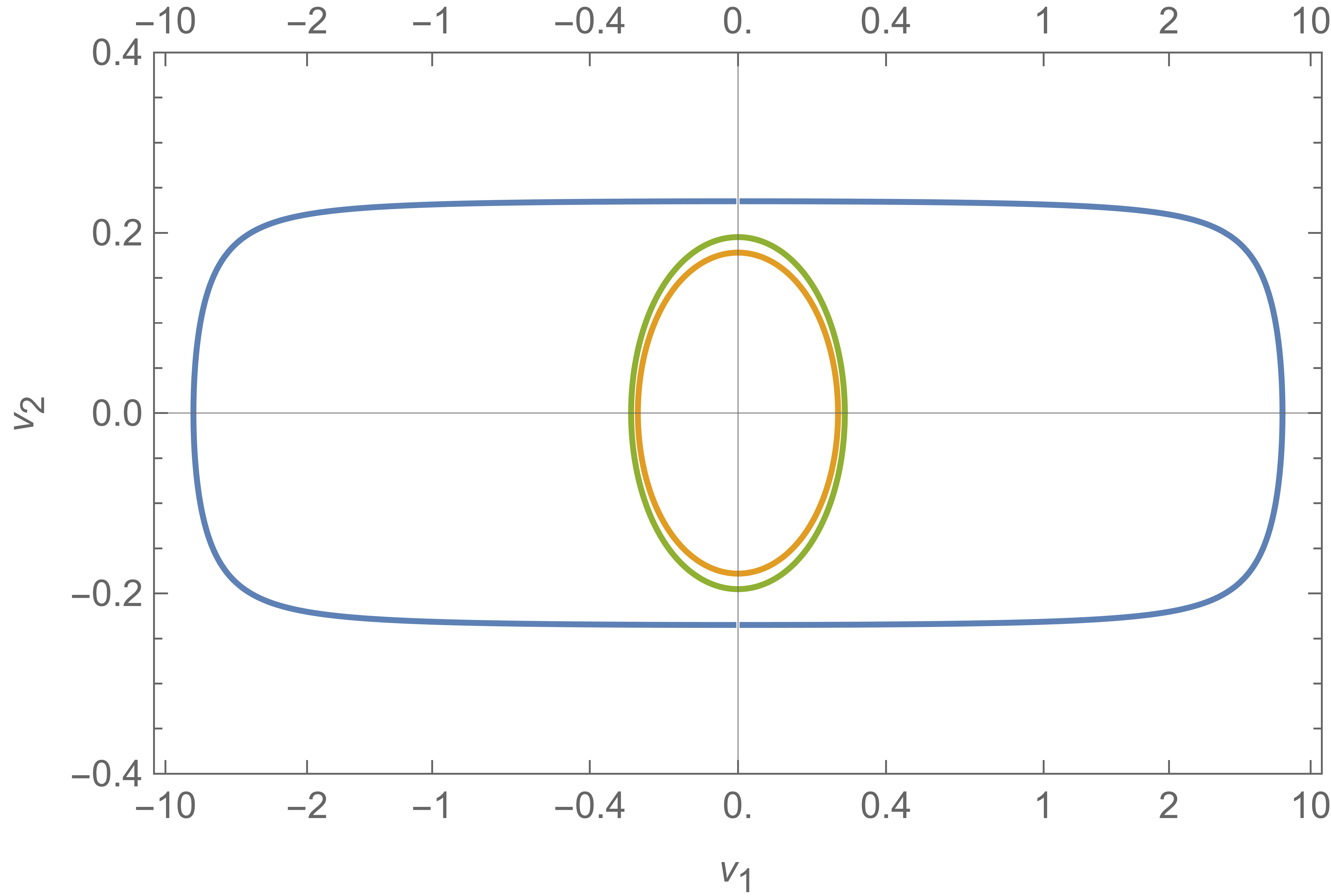
(a) $\mu=0.5$, $\sigma=0.2$

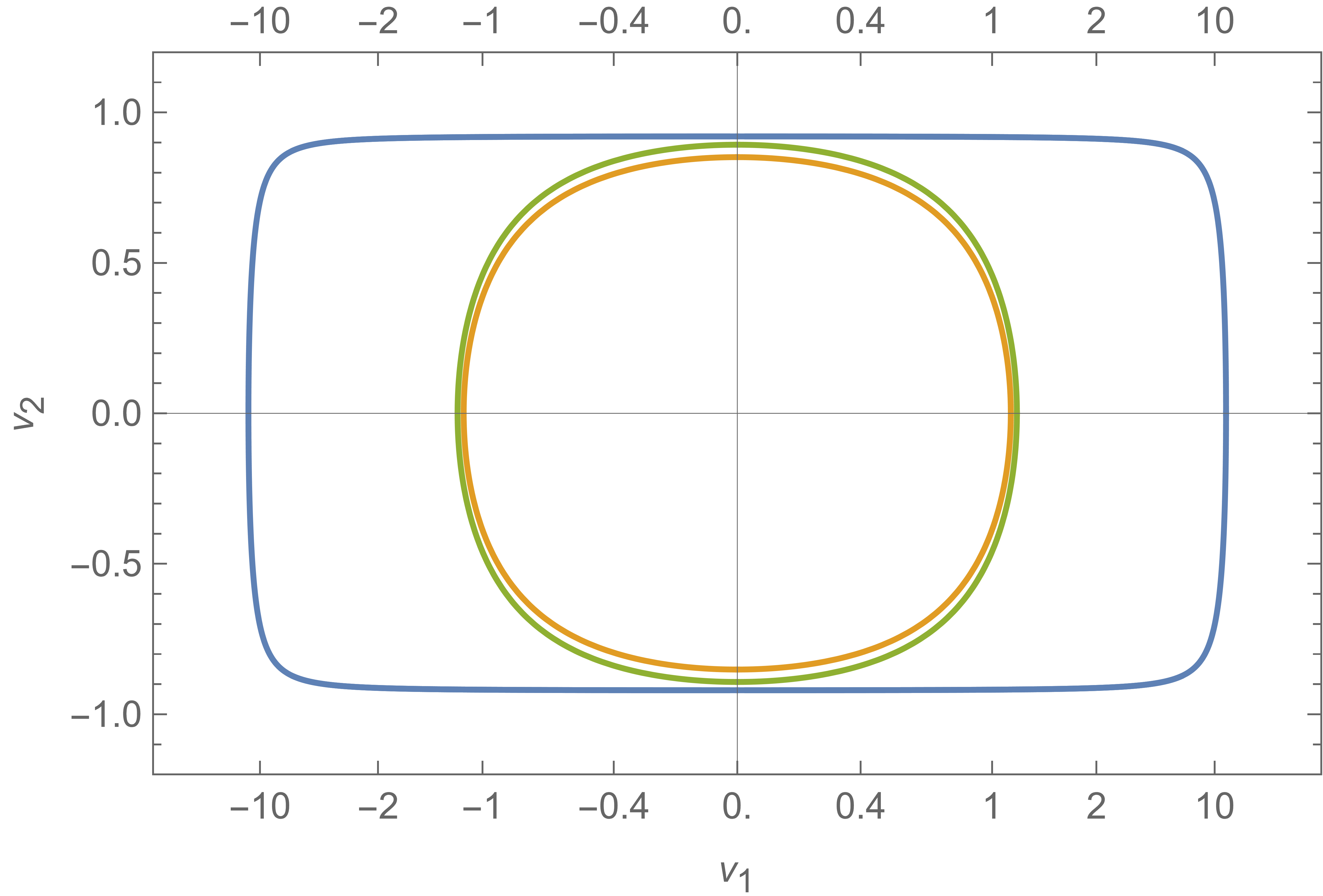
(b) $\mu=0.5$, $\sigma=0.3$

Figure 4: Asymptotic confidence regions for the estimators of the truncated normal distribution $TN(\mu,\sigma^{2})$ for $q=0.95$, $a=0$ and $b=1$ in the directions of the eigenvectors $v_{1}$ and $v_{2}$. Plotted are the MLE , the moment estimator and the Stein estimator . On the $x$-axis the scale is transformed via $x\mapsto\arctan x$.

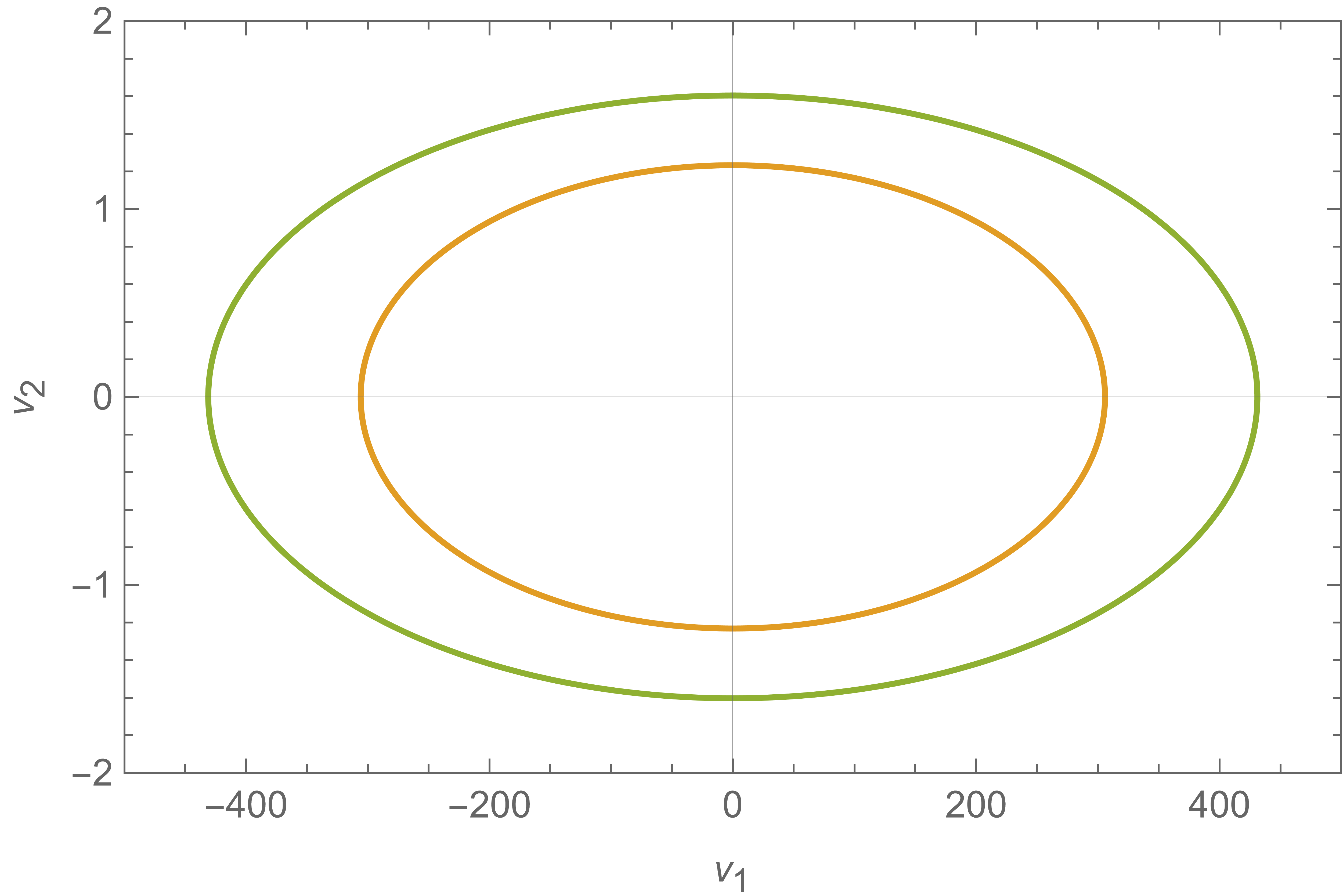
(c) $\alpha=0.5$, $\beta=3$

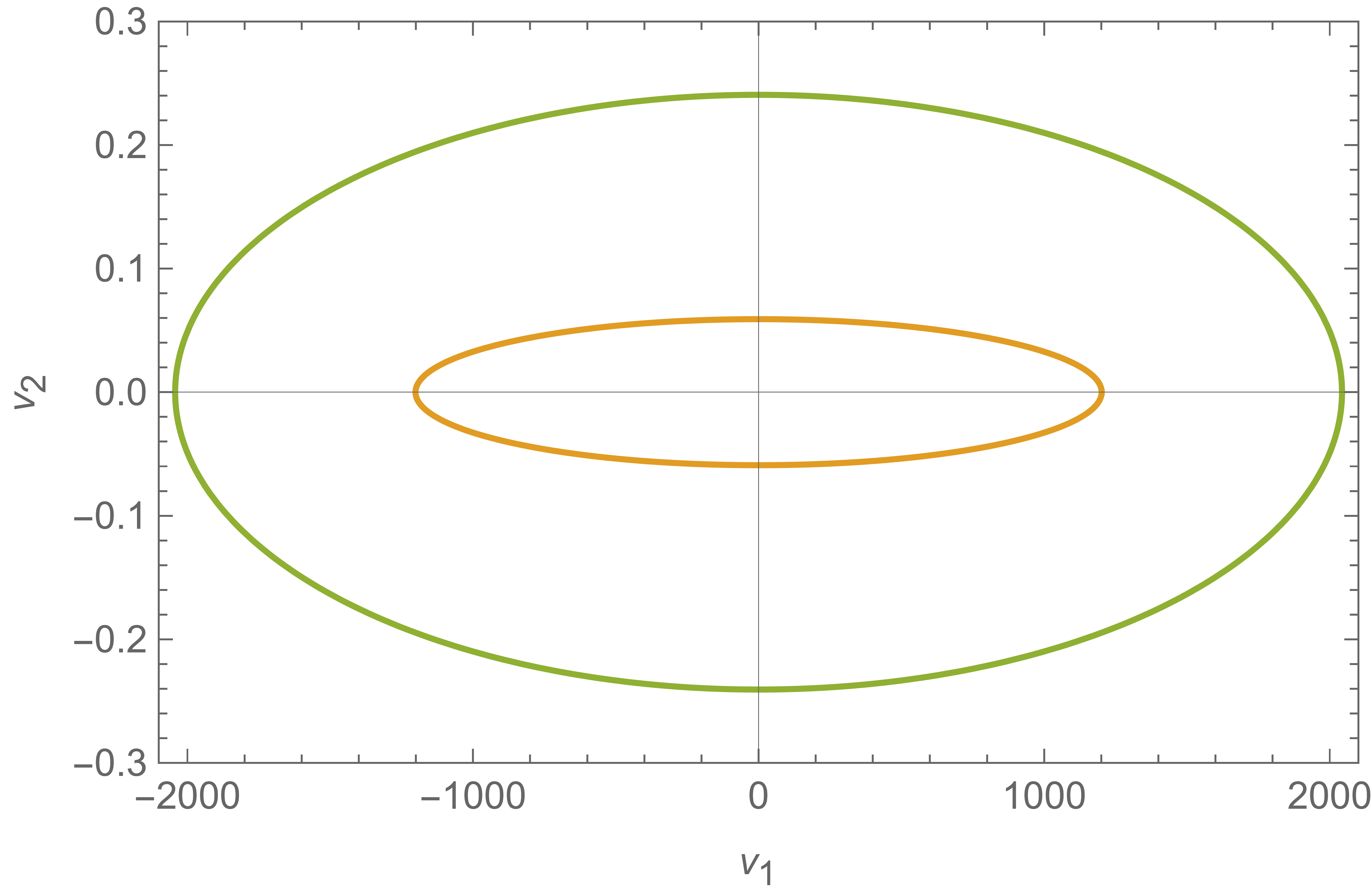
(d) $\alpha=0.1$, $\beta=4$

Figure 5: Asymptotic confidence regions for the estimators of the truncated inverse-gamma distribution $TIG(\alpha,\beta)$ for $q=0.95$ and $a=1$ in the directions of the eigenvectors $v_{1}$ and $v_{2}$. Plotted are the MLE $\hat{\theta}_{n}^{\mathrm{ML}}$ and the Stein estimator $\hat{\theta}_{n}^{\mathrm{ST}}$ .

3.8 Exponential polynomial models

For $\theta=(\theta_{1},\ldots,\theta_{p})\in\mathbb{R}^{p-1}\times(-\infty,0)$, the density of an exponential polynomial model is given by

$$p_{\theta}(x)=\frac{1}{C(\theta)}\exp(\theta_{1}x+\ldots+\theta_{p}x^{p}),\quad x>0,$$

where $C(\theta)=\int_{0}^{\infty}\exp(\theta_{1}x+\ldots+\theta_{p}x^{p})\,dx$ is the normalizing constant that cannot be calculated explicitly. We simply choose $\tau_{\theta}(x)=1$ and obtain

$$\mathcal{A}_{\theta}f(x)=(\theta_{1}+2\theta_{2}x+\ldots+p\theta_{p}x^{p-1})f(x)+f^{\prime}(x).$$

Here we choose $p$ test functions $f_{1},\ldots,f_{p}$. The Stein estimator is the solution to a system of linear equations, and we obtain

$$\hat{\theta}_{n}=A^{-1}b,$$

where

$$A=\begin{pmatrix}\overline{f_{1}(X)}&\ldots&p\overline{X^{p-1}f_{1}(X)}\\ \vdots&\ddots&\vdots\\ \overline{f_{p}(X)}&\ldots&p\overline{X^{p-1}f_{p}(X)}\end{pmatrix},\quad b=\begin{pmatrix}-\overline{f_{1}^{\prime}(X)}\\ \vdots\\ -\overline{f_{p}^{\prime}(X)}\end{pmatrix}.$$

We propose the obvious test functions $f_{1}(x)=x,\ldots,f_{p}(x)=x^{p}$, and denote the corresponding estimator by $\hat{\theta}_{n}^{\mathrm{ST1}}$. Another set of test functions which we consider is $f_{i}(x)=x^{i}e^{-ix}$, for $i=0,\ldots,p-1$. We call the respective Stein estimator $\hat{\theta}_{n}^{\mathrm{ST2}}$. Further, we also want to study the two-step estimator, which we denote by $\hat{\theta}_{n}^{\mathrm{ST3}}$, whereby we take $\hat{\theta}_{n}^{\mathrm{ST2}}$ as a first-step estimate. The conditions in order to verify consistency and asymptotic efficiency (Theorems 2.11 and 2.12) can be verified in a similar manner as in Section 3.1.

Let us now walk through the available estimation methods in the literature. The noise-contrastive estimator developed in [32] (a refined version of one of [31]) is defined as follows. We take the exponential distribution $E(\lambda)$ with parameter $\lambda$ and density $p_{\lambda}(x)=\lambda e^{-\lambda x}$, $x>0$, as the noise distribution and generate an i.i.d. sample, denoted by $Y_{1},\ldots,Y_{d}\sim E(\lambda)$. We choose the rate parameter $\lambda=1/\overline{X}$. Moreover, we take the tuning parameter $\nu=10$, which gives $d=10n$ for the sample size of the noise distribution. Letting $G_{\theta,\lambda}(x)=\log p_{\theta}(x)-\log p_{\lambda}(x)$ and $r_{\nu}(x)=\frac{1}{1+\nu\exp(-x)}$, the noise-contrastive estimator maximizes the quantity

$$J(\theta)=\frac{1}{n}\bigg{(}\sum_{i=1}^{n}\log r_{\nu}(G_{\theta,\lambda}(X_{i}))+\sum_{i=1}^{d}\log\big{(}1-r_{\nu}(G_{\theta,\lambda}(Y_{i})\big{)}\bigg{)}.$$

We write $\hat{\theta}_{n}^{\mathrm{NC}}$ for the estimator calculated by the latter method. Moreover, we consider the score matching approach in [39] (a refined version of one of [40]). This boils down to finding the minimum of

$$JJ(\theta) =\frac{1}{n}\sum_{i=1}^{n}\bigg{(}2X_{i}\frac{p_{\theta}^{\prime}(X_{i})}{p_{\theta}(X_{i})}+\frac{p_{\theta}^{\prime\prime}(X_{i})}{p_{\theta}(X_{i})}X_{i}^{2}+\frac{1}{2}\frac{p_{\theta}^{\prime}(X_{i})^{2}}{p_{\theta}(X_{i})^{2}}X_{i}^{2}\bigg{)}$$

$$=\frac{1}{n}\sum_{i=1}^{n}\bigg{(}\sum_{j=1}^{p}j(j+1)\theta_{j}X_{i}^{j}+\frac{1}{2}\bigg{(}\sum_{j=1}^{p}j\theta_{j}X_{i}^{j}\bigg{)}^{2}\bigg{)}.$$

We write $\hat{\theta}_{n}^{\mathrm{SM}}$. We remark that neither the score matching approach nor the noise-constrastive estimator is explicit and need to be computed via numerical optimization. In [37] and [49], the holomorphic gradient method is used in order to compute the MLE. We remark that for exponential polynomial models the MLE coincides with the moment estimators. To conclude, we implement the minimum $L^{q}$-estimator obtained in [9]. The latter are interestingly also motivated by a Stein characterization of the underlying probability distribution; more precisely, by an expectation-based representation of the cdf. This estimator, which we denote by $\hat{\theta}_{n}^{\mathrm{MD}}$, is calculated as follows. Let

$$\eta_{n}(t,\theta) =-\frac{1}{n}\sum_{i=1}^{n}\frac{p_{\theta}^{\prime}(X_{i})}{p_{\theta}(X_{i})}\min(t,X_{i})-\frac{1}{n}\sum_{i=1}^{n}1\{X_{i}\leq t\}$$

$$=-\frac{1}{n}\sum_{i=1}^{n}\min(t,X_{i})\sum_{j=1}^{p}j\theta_{j}x^{j-1}-\frac{1}{n}\sum_{i=1}^{n}1\{X_{i}\leq t\}.$$

Then $\hat{\theta}_{n}^{\mathrm{MD}}=\operatorname*{arg\,min}\{\|\eta_{n}(\cdot,\theta)\|_{\mathscr{L}^{q}}\,|\,\theta\in\Theta\}$, where $\|\cdot\|_{\mathscr{L}^{q}}$, $1\leq q<\infty$, is the $\mathscr{L}^{q}$-norm defined for a function $f:\mathbb{R}_{+}\rightarrow\mathbb{R}$ by

$$\|f\|_{\mathscr{L}^{q}}=\bigg{(}\int_{0}^{\infty}|f(t)|^{q}w(t)dt\bigg{)}^{1/q},$$

for a positive and integrable weight function $w:\mathbb{R}_{+}\rightarrow\mathbb{R}$. The authors recommend $q=2$, $w(t)=e^{-at}$ and the tuning parameter $a=1$ seems to produce the best results based on their simulations. We point out that the minimum-distance estimator $\hat{\theta}_{n}^{\mathrm{MD}}$ is only explicit for a parameter space of dimension less than or equal to $2$.

Simulation results regarding the bias, the MSE and existence of the estimators can be found in Tables 9 and 10 for sample size $n=1000$. We excluded the minimum distance estimator $\hat{\theta}_{n}^{\mathrm{MD}}$ from the study, since the numerical calculation with weight function and tuning parameter chosen as described above turns out to be too heavy for a parameter space dimension of $3$ or higher. For the MLE, $C(\theta)$ is calculated through numerical integration and then optimizing the log-likelihood function is performed with the Nelder-Mead algorithm. The vector $(-1,\ldots,-1)^{\top}\in\mathbb{R}^{p}$ is used as an initial guess for the optimization procedure. This implementation seems, at least for the parameter constellations we consider, to be computationally not too expensive and numerically stable. For the noise-contrastive estimator $\hat{\theta}_{n}^{\mathrm{NC}}$ and the score matching approach $\hat{\theta}_{n}^{\mathrm{SM}}$, we also use the Nelder-Mead algorithm with initial guess $(-1,\ldots,-1)^{\top}\in\mathbb{R}^{p}$. Note that for the two-step Stein estimator $\hat{\theta}_{n}^{\mathrm{ST3}}$, the normalizing constant $C(\theta)$ needs to be calculated in order to evaluate the optimal function. This is then done as for the other examples through numerical differentiation.

The column NE has to be interpreted as follows. First, the last element of the parameter vector $\theta_{p}$ has to be negative, thus if any estimator returns a positive value for the this parameter, we count the estimator as non-existent. Secondly, we restrict the computation time for each estimator to $20$ seconds meaning that an estimator counts equally as non-existent if it requires more time to be calculated or if the numerical procedure fails completely. Concerning $\hat{\theta}_{n}^{\mathrm{ST3}}$, we also used the parameter vector $(-1,\ldots,-1)^{\top}\in\mathbb{R}^{p}$ as a first-step estimate if $\hat{\theta}_{n}^{\mathrm{ST2}}$ was not available for a Monte Carlo sample. The sample size for this simulation was chosen to be larger than for the other simulation studies, since we are concerned with an estimation problem in which the variance of the estimator becomes typically large as the dimension of the parameter space grows. This makes it difficult to compare estimators for small sample sizes in the case of parameter dimensions of $3$ and $4$. Additionally, the Stein estimators $\hat{\theta}_{n}^{\mathrm{ST1}}$ and $\hat{\theta}_{n}^{\mathrm{ST2}}$ often return positive values for $\theta_{p}$, which makes a comparison even more difficult since the number of samples on which the bias and MSE are based is in truth lower than the number of Monte Carlo repetitions. However, for rather small sample sizes of $n=20$ or $n=50$, we found that our simulation results are reliable for a parameter space dimension of $2$ with similar results as described below, which is why we did not include a separate table for these results. Nevertheless, we now consider $n=1000$, where we feel more comfortable in drawing conclusions out of the study and observe a quite solid performance for the Stein estimators. For example, the explicit Stein estimators $\hat{\theta}_{n}^{\mathrm{ST1}}$ and $\hat{\theta}_{n}^{\mathrm{ST2}}$ outperform all other methods for the parameter vector $(-2,0.1,3,-2)^{\top}$ in terms of bias and MSE, although $\hat{\theta}_{n}^{\mathrm{ML}}$ and $\hat{\theta}_{n}^{\mathrm{NC}}$ remain to be globally the best. The two-step estimator $\hat{\theta}_{n}^{\mathrm{ST3}}$ can often improve in terms of bias and MSE with respect to the first-step estimator $\hat{\theta}_{n}^{\mathrm{ST2}}$ (although there are some exceptions). In the end, we advise to use the MLE or the noise-contrastive estimator $\hat{\theta}_{n}^{\mathrm{NC}}$, while the explicit Stein estimators can serve as a quite reliable initial guess, if existent.

$\theta_{0}$		Bias
		$\hat{\theta}_{n}^{\mathrm{ML}}$	$\hat{\theta}_{n}^{\mathrm{NC}}$	$\hat{\theta}_{n}^{\mathrm{SM}}$	$\hat{\theta}_{n}^{\mathrm{ST1}}$	$\hat{\theta}_{n}^{\mathrm{ST2}}$	$\hat{\theta}_{n}^{\mathrm{ST3}}$
$(1,-2)$	$\theta_{1}$	$0.02$	$0.019$	$0.085$	$0.03$	$0.03$	$0.017$
	$\theta_{2}$	$-0.017$	$-0.017$	$-0.055$	$-0.024$	$-0.024$	$-0.015$
$(-2,-1)$	$\theta_{1}$	$0.025$	$0.026$	$0.13$	$0.035$	$0.035$	$0.023$
	$\theta_{2}$	$-0.031$	$-0.032$	$-0.106$	$-0.04$	$-0.04$	$-0.029$
$(1,2,-3)$	$\theta_{1}$	$-0.025$	$-0.027$	$-0.477$	$-0.122$	$-0.122$	$-0.011$
	$\theta_{2}$	$0.073$	$0.079$	$0.737$	$0.244$	$0.244$	$0.042$
	$\theta_{3}$	$-0.051$	$-0.054$	$-0.34$	$-0.134$	$-0.134$	$-0.033$
$(-3,5,-1)$	$\theta_{1}$	$2.6$	$2.59$	$-4.83$	$-0.078$	$-0.078$	$2.82$
	$\theta_{2}$	$-0.92$	$-0.923$	$1.62$	$0.048$	$0.048$	$-0.986$
	$\theta_{3}$	$0.107$	$0.107$	$-0.18$	$-7.71\text{e-3}$	$-7.71\text{e-3}$	$0.113$
$(0.2,-0.8,-2)$	$\theta_{1}$	$-0.048$	$-0.054$	$-0.923$	$-0.208$	$-0.189$	$-0.093$
	$\theta_{2}$	$0.156$	$0.176$	$1.83$	$0.532$	$0.491$	$0.252$
	$\theta_{3}$	$-0.127$	$-0.142$	$-1.04$	$-0.359$	$-0.336$	$-0.183$
$(3,0.5,-0.5)$	$\theta_{1}$	$-0.018$	$0.019$	$-0.332$	$-0.101$	$-0.101$	$0.052$
	$\theta_{2}$	$0.026$	$-5.63\text{e-4}$	$0.205$	$0.075$	$0.075$	$-0.026$
	$\theta_{3}$	$-7.56\text{e-3}$	$-1.87\text{e-3}$	$-0.04$	$-0.016$	$-0.016$	$3.63\text{e-3}$
$(0.1,2,-3)$	$\theta_{1}$	$-0.036$	$-0.04$	$-0.544$	$-0.136$	$-0.136$	$-0.022$
	$\theta_{2}$	$0.102$	$0.112$	$0.909$	$0.296$	$0.295$	$0.067$
	$\theta_{3}$	$-0.07$	$-0.077$	$-0.445$	$-0.172$	$-0.171$	$-0.049$
$(3,0,-4)$	$\theta_{1}$	$-0.018$	$-0.021$	$-0.745$	$-0.164$	$-0.16$	$-5.05\text{e-3}$
	$\theta_{2}$	$0.088$	$0.093$	$1.38$	$0.391$	$0.382$	$0.049$
	$\theta_{3}$	$-0.082$	$-0.085$	$-0.763$	$-0.258$	$-0.253$	$-0.054$
$(1,2,0.5,-2)$	$\theta_{1}$	$-0.881$	$-0.94$	$3.42$	$1.16$	$0.888$	$0.58$
	$\theta_{2}$	$2.19$	$2.34$	$-7.61$	$-3.14$	$-2.43$	$-1.65$
	$\theta_{3}$	$-2.01$	$-2.16$	$6.73$	$3.15$	$2.48$	$1.71$
	$\theta_{4}$	$0.614$	$0.66$	$-2.06$	$-1.06$	$-0.842$	$-0.591$
$(-2,0.1,3,-2)$	$\theta_{1}$	$1.2$	$1.57$	$1.9$	$0.382$	$0.344$	$0.139$
	$\theta_{2}$	$-3.21$	$-4.2$	$-4.51$	$-1.19$	$-1.08$	$-0.43$
	$\theta_{3}$	$3.04$	$3.97$	$4.01$	$1.26$	$1.14$	$0.458$
	$\theta_{4}$	$-0.939$	$-1.22$	$-1.19$	$-0.421$	$-0.386$	$-0.159$

Table 9: Simulation results regarding the bias for the exponential polynomial models for $n=1000$ and $10,000$ repetitions.

$\theta_{0}$		MSE						NE
		$\hat{\theta}_{n}^{\mathrm{ML}}$	$\hat{\theta}_{n}^{\mathrm{NC}}$	$\hat{\theta}_{n}^{\mathrm{SM}}$	$\hat{\theta}_{n}^{\mathrm{ST1}}$	$\hat{\theta}_{n}^{\mathrm{ST2}}$	$\hat{\theta}_{n}^{\mathrm{ST3}}$	$\hat{\theta}_{n}^{\mathrm{ML}}$	$\hat{\theta}_{n}^{\mathrm{NC}}$	$\hat{\theta}_{n}^{\mathrm{SM}}$	$\hat{\theta}_{n}^{\mathrm{ST1}}$	$\hat{\theta}_{n}^{\mathrm{ST2}}$	$\hat{\theta}_{n}^{\mathrm{ST3}}$
$(1,-2)$	$\theta_{1}$	$0.073$	$0.079$	$0.28$	$0.09$	$0.09$	$0.073$	$0$	$0$	$0$	$0$	$0$	$0$
	$\theta_{2}$	$0.039$	$0.042$	$0.109$	$0.047$	$0.047$	$0.039$
$(-2,-1)$	$\theta_{1}$	$0.084$	$0.092$	$0.289$	$0.09$	$0.09$	$0.084$	$0$	$0$	$0$	$0$	$0$	$0$
	$\theta_{2}$	$0.069$	$0.074$	$0.171$	$0.074$	$0.074$	$0.068$
$(1,2,-3)$	$\theta_{1}$	$0.687$	$0.743$	$4.83$	$1.15$	$1.15$	$0.687$	$0$	$0$	$0$	$0$	$0$	$0$
	$\theta_{2}$	$2.08$	$2.26$	$10.7$	$3.4$	$3.4$	$2.08$
	$\theta_{3}$	$0.533$	$0.576$	$2.12$	$0.834$	$0.834$	$0.532$
$(-3,5,-1)$	$\theta_{1}$	$6.74$	$6.73$	$44.8$	$39.6$	$39.6$	$29.4$	$0$	$0$	$0$	$0$	$0$	$0$
	$\theta_{2}$	$0.873$	$0.882$	$5.29$	$4.99$	$4.99$	$3.7$
	$\theta_{3}$	$0.013$	$0.013$	$0.069$	$0.068$	$0.068$	$0.051$
$(0.2,-0.8,-2)$	$\theta_{1}$	$0.675$	$0.725$	$3.8$	$0.839$	$0.871$	$0.62$	$0$	$0$	$9$	$3$	$3$	$1$
	$\theta_{2}$	$3.46$	$3.72$	$14.8$	$4.43$	$4.57$	$3.16$
	$\theta_{3}$	$1.42$	$1.51$	$4.85$	$1.82$	$1.86$	$1.31$
$(3,0.5,-0.5)$	$\theta_{1}$	$0.873$	$0.769$	$3.82$	$1.38$	$1.38$	$0.67$	$0$	$0$	$0$	$0$	$0$	$0$
	$\theta_{2}$	$0.402$	$0.345$	$1.35$	$0.565$	$0.565$	$0.292$
	$\theta_{3}$	$0.018$	$0.015$	$0.047$	$0.023$	$0.023$	$0.013$
$(0.1,2,-3)$	$\theta_{1}$	$0.636$	$0.681$	$4.23$	$0.967$	$0.968$	$0.636$	$0$	$0$	$1$	$0$	$0$	$0$
	$\theta_{2}$	$2.31$	$2.48$	$11.1$	$3.48$	$3.49$	$2.31$
	$\theta_{3}$	$0.684$	$0.73$	$2.53$	$0.996$	$0.997$	$0.681$
$(3,0,-4)$	$\theta_{1}$	$1.08$	$1.17$	$6.92$	$1.77$	$1.78$	$1.08$	$0$	$0$	$2$	$0$	$0$	$0$
	$\theta_{2}$	$4.75$	$5.18$	$22.4$	$7.55$	$7.6$	$4.71$
	$\theta_{3}$	$1.78$	$1.94$	$6.59$	$2.71$	$2.73$	$1.77$
$(1,2,0.5,-2)$	$\theta_{1}$	$1.34$	$1.27$	$33.2$	$6.71$	$7.23$	$3.31$	$0$	$0$	$16$	$13$	$9$	$1$
	$\theta_{2}$	$9.3$	$8.96$	$161$	$45.2$	$48.7$	$21.6$
	$\theta_{3}$	$10.2$	$10$	$128$	$44.2$	$47.2$	$21.6$
	$\theta_{4}$	$1.29$	$1.28$	$12.3$	$4.93$	$5.22$	$2.51$
$(-2,0.1,3,-2)$	$\theta_{1}$	$2.61$	$3.2$	$13.8$	$1.94$	$2.02$	$2.54$	$0$	$0$	$9$	$2$	$1$	$0$
	$\theta_{2}$	$19.9$	$24.2$	$78$	$16.4$	$17.1$	$21.4$
	$\theta_{3}$	$18.9$	$22.9$	$62$	$17$	$17.7$	$22$
	$\theta_{4}$	$1.9$	$2.31$	$5.54$	$1.83$	$1.9$	$2.34$

Table 10: Simulation results regarding the MSE and existence for the exponential polynomial models for $n=1000$ and $10,000$ repetitions.

3.9 Cauchy distribution

For $\theta=(\mu,\gamma)\in\mathbb{R}\times(0,\infty)$, the density the Cauchy distribution is given by

$$p_{\theta}(x)=\bigg{(}\pi\gamma\bigg{(}1+\bigg{(}\frac{x-\mu}{\gamma}\bigg{)}^{2}\bigg{)}\bigg{)}^{-1},\quad x\in\mathbb{R}.$$

We choose $\tau_{\theta}=(x-\mu)^{2}+\gamma^{2}$ and obtain

$$\mathcal{A}_{\theta}f(x)=\big{(}(x-\mu)^{2}+\gamma^{2}\big{)}f^{\prime}(x)$$

(see [56]). We choose two test functions $f_{1}$, $f_{2}$ and calculate the estimators

$$\hat{\mu}_{n}= \frac{1}{2}\frac{\overline{f_{2}^{\prime}(X)}\ \overline{X^{2}f_{1}^{\prime}(X)}-\overline{f_{1}^{\prime}(X)}\ \overline{X^{2}f_{2}^{\prime}(X)}}{\overline{f_{2}^{\prime}(X)}\ \overline{Xf_{1}^{\prime}(X)}-\overline{f_{1}^{\prime}(X)}\ \overline{Xf_{2}^{\prime}(X)}},$$ (27)

$$\hat{\gamma}_{n}^{2}= \frac{\overline{X^{2}f_{2}^{\prime}(X)}\ \overline{Xf_{1}^{\prime}(X)}-\overline{X^{2}f_{1}^{\prime}(X)}\ \overline{Xf_{2}^{\prime}(X)}}{\overline{f_{1}^{\prime}(X)}\ \overline{Xf_{2}^{\prime}(X)}-\overline{f_{2}^{\prime}(X)}\ \overline{Xf_{1}^{\prime}(X)}}-\hat{\mu}_{n}^{2}.$$ (28)

We benefit from a simple cdf, which is given by $P_{\theta}(x)=\frac{1}{\pi}\arctan\big{(}\frac{x-\mu}{\gamma}\big{)}+\frac{1}{2}$. We compute the optimal functions as follows:

$$f_{\theta}^{(1)}(x)=-\frac{1}{\gamma^{2}+(x-\mu)^{2}}\quad\text{and}\quad f_{\theta}^{(2)}(x)=\frac{\mu-x}{\gamma\big{(}\gamma^{2}+(x-\mu)^{2}\big{)}}.$$ (29)

We emphasize that all necessary assumptions in order to apply Theorems 2.11 are 2.12 are satisfied and with a suitable fist step estimate, we have an efficient estimator which is considerably simpler to compute than the MLE, which requires to solve the equations

$$\sum_{i=1}^{n}\frac{2(X_{i}-\mu)}{\gamma^{2}+(X_{i}-\mu)^{2}}=0\quad\text{and}\quad\frac{n}{\gamma}-\sum_{i=1}^{n}\frac{2\gamma}{\gamma^{2}+(X_{i}-\mu)^{2}}=0,$$

which is equivalent to solving a polynomial equation of degree $2n-1$. [17] and [24] showed that in the case in which $\mu$ and $\gamma$ are unknown, the likelihood function is unimodal and the MLE can be obtained easily through numerical integration. We accentuate that moment estimation is not tractable due to the non-existence of all moments.

Interestingly, parameter estimation for the Cauchy distribution is more difficult in the case where $\gamma$ is known and one wants to estimate the location parameter $\mu$, which is why we focus on this scenario and consider from now on $\gamma$ as known. This means our parameter space reduces to $\Theta=\mathbb{R}$ with $\theta=\mu$. The estimation in the latter case has received great attention in the literature; se [63] for an overview of available estimation techniques. The MLE of $\mu$ with known $\gamma$ is often cited as an example of computational failure (see [4]), except for sample sizes $3$ and $4$ (see [21]). The reason for this is a multimodal (one-dimensional) likelihood function (in fact the number of local maxima is asymptotically Poisson distributed with mean $1/\pi$; see, for example, [5]). Also, the MLE is inefficient for small sample sizes (see [54] or [6]). Therefore, other methods have been developed, such as L-estimation. To this end, let $X_{(1)},\ldots,X_{(n)}$ be the order statistic of $X_{1},\ldots,X_{n}$. In [55], the authors showed that it can be more efficient to use only a part of the observations due to the heavy tails of the Cauchy distribution, and proposed the estimator

$$\hat{\mu}_{n}^{\mathrm{L1}}=\frac{1}{n-2r}\sum_{i=r+1}^{n-r}X_{(i)},$$

where $r=\lfloor np\rfloor$, $0<p<0.5$, with $p=0.38$ recommended in order to achieve a minimal variance. [10] developed an L-estimator based on only $5$ order statistics, defined by

$$\hat{\mu}_{n}^{\mathrm{L2}}=\sum_{i=1}^{5}\omega_{i}X_{(\lfloor np_{i}\rfloor)},$$

and found $(p_{1},p_{2},p_{3},p_{4},p_{5})=(0.13,0.4,0.5,0.6,0.87)$ and $(\omega_{1},\omega_{2},\omega_{3},\omega_{4},\omega_{5})=(-0.052,0.3485,0.407,0.3485,-0.052)$ to be optimal. Another asymptotically efficient estimator was developed in [16]:

$$\hat{\mu}_{n}^{\mathrm{L3}}=\frac{1}{n}\sum_{i=1}^{n}J\bigg{(}\frac{i}{n+1}\bigg{)}X_{(i)},$$

where $J(u)=\sin\big{(}4\pi(u-0.5)\big{)}/\tan\big{(}\pi(u-0.5)\big{)}$. Furthermore, [63] proposed to modify the latter estimator in order to also achieve a high efficiency for finite sample sizes and obtained the estimator $\hat{\mu}_{n}^{\mathrm{L4}}=\sum_{i=1}^{n}\omega_{i}X_{(i)}$, where $\omega_{i}=c^{-1}\big{(}\cos\big{(}\pi\big{(}\frac{i-0.5}{n}-0.5\big{)}\big{)}\big{)}^{2+\epsilon_{n}}\cos\big{(}2\pi\big{(}\frac{i-0.5}{n}-0.5\big{)}\big{)}$, $c\in\mathbb{R}$, are such that $\sum_{i=1}^{n}\omega_{i}=1$. The constant $\epsilon_{n}$ needs to be chosen such that the estimator is efficient for the corresponding sample size $n$. The authors give propositions for certain values of $n$; in fact, $\epsilon_{n}$ should converge to $0$ as $n$ grows. If we choose $\epsilon_{n}=0$, we retrieve $\hat{\mu}_{n}^{\mathrm{L3}}$, which is asymptotically normal and therefore $\hat{\mu}_{n}^{\mathrm{L4}}$ is asymptotically normal as well. We also consider the Pitman estimator [23], given by

$$\hat{\mu}_{n}^{\mathrm{PI}}=\sum_{i=1}^{n}\frac{\mathrm{Re}(\omega_{i})}{\sum_{j=1}^{n}\mathrm{Re}(\omega_{j})}X_{i},$$

where

$$\omega_{k}=\prod_{j\neq k}\bigg{(}\frac{1}{(X_{k}-X_{j})^{2}+4\gamma^{2}}\bigg{)}\bigg{(}1-\frac{2\gamma}{X_{k}-X_{j}}\mathrm{i}\bigg{)}.$$

Note that in the latter formula, $\mathrm{i}$ represents the imaginary unit rather than an index.

Now, we describe the procedure that we propose. Note that if we choose one test function (since we only have to estimate $\mu$), the corresponding equation is quadratic and has in general two solutions. This is why we choose two test functions and consider the estimator (27). We take $\hat{\mu}_{n}^{\mathrm{L4}}$ as a first-step estimate and propose to use the optimal functions (29), whereby $\gamma$ is known. We give the derivatives:

$$\big{(}f_{\theta}^{(1)}\big{)}^{\prime}(x)=\frac{2(x-\mu)}{\big{(}\gamma^{2}+(x-\mu)^{2}\big{)}^{2}}\quad\text{and}\quad\big{(}f_{\theta}^{(2)}\big{)}^{\prime}(x)=\frac{(\gamma+x-\mu)(\gamma-x+\mu)}{\gamma\big{(}\gamma^{2}+(x-\mu)^{2}\big{)}^{2}},$$

and denote the resulting estimator by $\hat{\mu}_{n}^{\mathrm{ST1}}$. Note that $\hat{\mu}_{n}^{\mathrm{ST1}}$ is not translation-invariant and we therefore consider different values of $\mu$ in our simulation. As we will see in the sequel, this slight modification of the estimation procedure still results in an asymptotically efficient estimator. We compare its asymptotic variance to that of the MLE. We can make use of Theorem 2.11 (where we take $\tilde{\gamma}_{n}=\gamma_{0}$ as the first-step estimator for $\gamma$). Then the asymptotic variance of $\hat{\mu}_{n}^{\mathrm{ST1}}$ is exactly the top-left element of the inverse Fisher information matrix in the case where $\gamma$ is unknown. The latter is given by

$$I_{\mathrm{ML}}^{-1}(\mu,\gamma)=\begin{pmatrix}2\gamma^{2}&0\\ 0&2\gamma^{2}\end{pmatrix},$$

and we conclude that the asymptotic variance for both estimators $\hat{\mu}_{n}^{\mathrm{ST1}}$ and the (one-dimensional) MLE equals $2\gamma^{2}$. However, when performing the simulations we noticed a very large variance for $\hat{\mu}_{n}^{\mathrm{ST1}}$ for small sample sizes, which is consistent with the trade-off between small sample size and asymptotic efficiency noticed by [63] for $\hat{\mu}_{n}^{\mathrm{L3}}$ and $\hat{\mu}_{n}^{\mathrm{L4}}$. This is why we propose a modified version of $\hat{\mu}_{n}^{\mathrm{ST1}}$, denoted by $\hat{\mu}_{n}^{\mathrm{ST2}}$. In a similar manner to the estimator $\hat{\mu}_{n}^{\mathrm{L1}}$, we cut off the bottom and top $p$-quantile of the sample at hand and calculate the sample means in (27) by the means of the remaining observations. Pursuant to $\hat{\mu}_{n}^{\mathrm{L1}}$, we choose $p=0.38$ and disregard the first and last $r=\lfloor np\rfloor$ observations of the sorted sample. Simulation results can be found in Tables 11 and 12. For the sample size $n=20$, the Pitman estimator $\hat{\mu}_{n}^{\mathrm{PI}}$ seems to be globally the best, whereby for $n=50$ the modified L-estimator $\hat{\mu}_{n}^{\mathrm{L4}}$ appears to be very efficient as well. For the latter sample size, the Stein estimator $\hat{\mu}_{n}^{\mathrm{ST1}}$ outperforms all other estimators for some parameter constellations, whereby $\hat{\mu}_{n}^{\mathrm{ST1}}$ also show a competitive performance for $n=20$.

$\theta_{0}$		Bias					MSE
		$\hat{\mu}_{n}^{\mathrm{L1}}$	$\hat{\mu}_{n}^{\mathrm{L2}}$	$\hat{\mu}_{n}^{\mathrm{L4}}$	$\hat{\mu}_{n}^{\mathrm{PI}}$	$\hat{\mu}_{n}^{\mathrm{ST2}}$	$\hat{\mu}_{n}^{\mathrm{L1}}$	$\hat{\mu}_{n}^{\mathrm{L2}}$	$\hat{\mu}_{n}^{\mathrm{L4}}$	$\hat{\mu}_{n}^{\mathrm{PI}}$	$\hat{\mu}_{n}^{\mathrm{ST2}}$
$(-5,1)$	$\mu$	$-0.725$	$0.131$	$-2.54\text{e-3}$	$1.72\text{e-4}$	$0.085$	$0.721$	$0.944$	$0.136$	$0.116$	$0.158$
$(-4,1.5)$	$\mu$	$-0.506$	$0.193$	$-4.22\text{e-3}$	$-3.13\text{e-5}$	$0.122$	$0.695$	$1.04$	$0.307$	$0.261$	$0.351$
$(-2,2)$	$\mu$	$-0.099$	$0.261$	$8.84\text{e-3}$	$3.88\text{e-3}$	$0.182$	$0.782$	$2.26$	$0.537$	$0.46$	$0.627$
$(0,1)$	$\mu$	$0.118$	$0.117$	$5.1\text{e-3}$	$3.95\text{e-3}$	$0.091$	$0.206$	$0.296$	$0.134$	$0.113$	$0.161$
$(0,3)$	$\mu$	$0.343$	$0.394$	$5.14\text{e-3}$	$3.29\text{e-3}$	$0.273$	$1.87$	$4.81$	$1.22$	$1.02$	$1.42$
$(2,0.1)$	$\mu$	$0.345$	$0.013$	$3.05\text{e-4}$	$2.73\text{e-4}$	$9.01\text{e-3}$	$0.121$	$5.89\text{e-3}$	$1.36\text{e-3}$	$1.15\text{e-3}$	$1.59\text{e-3}$
$(2,0.5)$	$\mu$	$0.388$	$0.065$	$-1.29\text{e-3}$	$-1.22\text{e-3}$	$0.043$	$0.2$	$0.24$	$0.034$	$0.028$	$0.039$
$(4,0.8)$	$\mu$	$0.751$	$0.092$	$-4.79\text{e-3}$	$-4.02\text{e-3}$	$0.066$	$0.69$	$0.325$	$0.087$	$0.074$	$0.101$
$(6,2.3)$	$\mu$	$1.26$	$0.29$	$7.79\text{e-3}$	$3.64\text{e-3}$	$0.217$	$2.59$	$2.02$	$0.693$	$0.59$	$2.92$
$(10,0.2)$	$\mu$	$1.69$	$0.026$	$5.34\text{e-4}$	$3.58\text{e-4}$	$0.018$	$2.86$	$0.03$	$5.62\text{e-3}$	$4.49\text{e-3}$	$6.78\text{e-3}$

Table 11: Simulation results for the $C(\mu,\gamma)$ distribution for $n=20$ and $10,000$ repetitions.

$\theta_{0}$		Bias					MSE
		$\hat{\mu}_{n}^{\mathrm{L1}}$	$\hat{\mu}_{n}^{\mathrm{L2}}$	$\hat{\mu}_{n}^{\mathrm{L4}}$	$\hat{\mu}_{n}^{\mathrm{PI}}$	$\hat{\mu}_{n}^{\mathrm{ST1}}$	$\hat{\mu}_{n}^{\mathrm{L1}}$	$\hat{\mu}_{n}^{\mathrm{L2}}$	$\hat{\mu}_{n}^{\mathrm{L4}}$	$\hat{\mu}_{n}^{\mathrm{PI}}$	$\hat{\mu}_{n}^{\mathrm{ST1}}$
$(-5,1)$	$\mu$	$-0.378$	0.012	$1.63\text{e-3}$	$3.7\text{e-3}$	$1.71\text{e-3}$	0.201	0.048	0.05	0.082	0.044
$(-4,1.5)$	$\mu$	$-0.276$	0.015	$1.38\text{e-3}$	$1.5\text{e-3}$	$1.17\text{e-3}$	0.206	0.105	0.11	0.099	0.099
$(-2,2)$	$\mu$	$-0.092$	0.025	$-7.46\text{e-4}$	$7.45\text{e-3}$	$1.33\text{e-3}$	0.248	0.195	0.202	0.554	0.182
$(0,1)$	$\mu$	0.034	$7.29\text{e-3}$	$-2.69\text{e-3}$	$3.68\text{e-3}$	$-3.39\text{e-3}$	0.058	0.047	0.048	0.517	0.044
$(0,3)$	$\mu$	0.094	0.024	$-0.016$	$-9.89\text{e-3}$	$-0.01$	0.527	0.42	0.437	0.384	0.39
$(2,0.1)$	$\mu$	0.171	$1.29\text{e-3}$	$1.9\text{e-4}$	$4.96\text{e-4}$	$1.93\text{e-4}$	0.03	$4.79\text{e-4}$	$4.99\text{e-4}$	$1.08\text{e-3}$	$4.46\text{e-4}$
$(2,0.5)$	$\mu$	0.186	$6.37\text{e-3}$	$2.87\text{e-4}$	$1.14\text{e-3}$	$1.12\text{e-3}$	0.049	0.012	0.012	0.019	0.011
$(4,0.8)$	$\mu$	0.364	$8.99\text{e-3}$	$4.44\text{e-4}$	$-2.36\text{e-3}$	$-2.75\text{e-4}$	0.169	0.03	0.031	0.037	0.028
$(6,2.3)$	$\mu$	0.582	0.024	$-3.22\text{e-3}$	$-9.5\text{e-4}$	$-2.31\text{e-3}$	0.639	0.243	0.253	0.24	0.226
$(10,0.2)$	$\mu$	0.84	$1.84\text{e-3}$	$-4.34\text{e-4}$	$-2.94\text{e-3}$	$-2.73\text{e-4}$	0.708	$1.83\text{e-3}$	$1.87\text{e-3}$	0.154	$1.7\text{e-3}$

Table 12: Simulation results for the $C(\mu,\gamma)$ distribution for $n=50$ and $10,000$ repetitions.

3.10 Generalized logistic distribution

The density of the generalized logistic distribution $GL(\alpha,\beta)$ with $\theta=(\alpha,\beta)$, $\alpha,\beta>0$, is given by

$$p_{\theta}(x)=\frac{1}{B(\alpha,\beta)}\frac{e^{-\beta x}}{(1+e^{-x})^{\alpha+\beta}},\quad x\in\mathbb{R}.$$

We choose $\tau_{\theta}(x)=1+e^{x}$ and get

$$\mathcal{A}_{\theta}f(x)=\big{(}\alpha-e^{x}(\beta-1)\big{)}f(x)+(1+e^{x})f^{\prime}(x).$$

With two test functions $f_{1}$, $f_{2}$ we have the estimators

$$\hat{\alpha}_{n}= \frac{\overline{(1+e^{X})f_{2}^{\prime}(X)}\ \overline{e^{X}f_{1}(X)}-\overline{(1+e^{X})f_{1}^{\prime}(X)}\ \overline{e^{X}f_{2}(X)}}{\overline{e^{X}f_{2}(X)}\ \overline{f_{1}(X)}-\overline{e^{X}f_{1}(X)}\ \overline{f_{2}(X)}},$$

$$\hat{\beta}_{n}= \frac{\Big{(}\overline{(1+e^{X})f_{2}^{\prime}(X)}+\overline{e^{X}f_{2}(X)}\Big{)}\ \overline{f_{1}(X)}-\Big{(}\overline{(1+e^{X})f_{1}^{\prime}(X)}+\overline{e^{X}f_{1}(X)}\Big{)}\ \overline{f_{2}(X)}}{\overline{e^{X}f_{2}(X)}\ \overline{f_{1}(X)}-\overline{e^{X}f_{1}(X)}\ \overline{f_{2}(X)}}.$$

The first two moments are given by

$$\mathbb{E}[X]=\psi(\alpha)-\psi(\beta)\quad\text{and}\quad\mathbb{E}[X^{2}]=\psi^{\prime}(\alpha)+\psi^{\prime}(\beta)+(\psi(\alpha)-\psi(\beta))^{2}.$$

If existent, the moment estimator $\hat{\theta}_{n}^{\mathrm{MO}}=(\hat{\alpha}_{n}^{\mathrm{MO}},\hat{\beta}_{n}^{\mathrm{MO}})$ is defined as the solution of the empirical versions of the equations above. It is clear that the latter is not explicit. The MLE $\hat{\theta}_{n}^{\mathrm{ML}}=(\hat{\alpha}_{n}^{\mathrm{ML}},\hat{\beta}_{n}^{\mathrm{ML}})$ is defined as the values in $\Theta$, at which the log-likelihood function attains its maximum. Supposing the latter exists and is uniquely determined by the critical point of the derivative, the MLE is the solution to the equations

$$\overline{\log(1+e^{-X})}=\psi(\alpha)-\psi(\alpha+\beta)\quad\text{and}\quad\overline{X}+\overline{\log(1+e^{-X})}=\psi(\beta)-\psi(\alpha+\beta).$$

The Fisher information matrix can also be calculated and is given by

$$I_{\mathrm{ML}}(\alpha,\beta)=\begin{pmatrix}\psi^{\prime}(\alpha)-\psi^{\prime}(\alpha+\beta)&-\psi^{\prime}(\alpha+\beta)\\ -\psi^{\prime}(\alpha+\beta)&\psi^{\prime}(\beta)-\psi^{\prime}(\alpha+\beta)\end{pmatrix}.$$

Considering the Stein estimator $\hat{\theta}_{n}^{\mathrm{ST}}=(\hat{\alpha}_{n}^{\mathrm{ST}},\hat{\beta}_{n}^{\mathrm{ST}})$, we choose the test functions $f_{1}(x)=\frac{1}{1+e^{x}}$ and $f_{1}(x)=\frac{1}{(1+e^{x})^{2}}$ such that Assumptions 2.2(a)–(b) are easily verified. The results of the simulation study can be found in Tables 13 and 14. In order to calculate the moment estimators $\hat{\alpha}_{n}^{\mathrm{MO}}$ and $\hat{\beta}_{n}^{\mathrm{MO}}$, we employed the R function nleqslv from the R package nleqslv [36] with initial values $(1,1)$. The MLE are obtained through numerical optimization of the log-likelihood function (as well with initial guess $(1,1)$). Interestingly, the MLE – although asymptotically efficient – is outperformed by the moment estimators for most parameter constellations for sample sizes $n=20$ and $n=50$. The Stein estimator is competitive, in terms of MSE, mostly residing between the MLE and moment estimator. However, the Stein estimator is the only one among the considered estimation techniques that is completely explicit, and does not seem to generate estimates that lie outside of the parameter space, as can be seen in column NE.

$\theta_{0}$		Bias			MSE			NE
		$\hat{\theta}_{n}^{\mathrm{ML}}$	$\hat{\theta}_{n}^{\mathrm{MO}}$	$\hat{\theta}_{n}^{\mathrm{ST}}$	$\hat{\theta}_{n}^{\mathrm{ML}}$	$\hat{\theta}_{n}^{\mathrm{MO}}$	$\hat{\theta}_{n}^{\mathrm{ST}}$	$\hat{\theta}_{n}^{\mathrm{ML}}$	$\hat{\theta}_{n}^{\mathrm{MO}}$	$\hat{\theta}_{n}^{\mathrm{ST}}$
$(1,1)$	$\alpha$	0.182	0.157	0.132	0.195	0.18	0.189	0	0	0
	$\beta$	0.178	0.153	0.129	0.196	0.181	0.191
$(0.4,1)$	$\alpha$	0.083	0.05	0.055	0.027	0.021	0.034	9	0	0
	$\beta$	0.311	0.19	0.18	0.442	0.268	0.35
$(0.8,1.5)$	$\alpha$	0.136	0.115	0.111	0.114	0.105	0.126	0	0	0
	$\beta$	0.314	0.259	0.239	0.572	0.49	0.551
$(3,1)$	$\alpha$	0.662	0.551	0.592	2.51	2.15	2.73	0	0	0
	$\beta$	0.171	0.147	0.165	0.183	0.166	0.22
$(0.2,3)$	$\alpha$	0.094	0.021	0.08	0.016	$4\text{e-3}$	0.024	81	0	0
	$\beta$	3.46	1.23	2.34	44.3	10.3	28.1
$(4,6)$	$\alpha$	0.71	0.686	0.651	3.39	3.34	3.33	0	0	0
	$\beta$	1.1	1.06	1.01	7.92	7.79	7.76
$(7,0.5)$	$\alpha$	2.98	1.7	2.88	35.4	18.6	38.3	21	0	0
	$\beta$	0.102	0.064	0.142	0.047	0.032	0.09
$(0.2,8)$	$\alpha$	0.108	0.021	0.104	0.02	$4\text{e-3}$	0.031	90	0	0
	$\beta$	10.1	3.28	7.95	333	61.5	297
$(3,10)$	$\alpha$	0.511	0.48	0.501	1.77	1.71	1.87	0	0	0
	$\beta$	1.85	1.73	1.79	22.6	21.7	23.6
$(0.5,0.4)$	$\alpha$	0.118	0.075	0.062	0.065	0.046	0.056	10	0	0
	$\beta$	0.083	0.051	0.044	0.029	0.024	0.032

Table 13: Simulation results for the $GL(\alpha,\beta)$ distribution for $n=20$ and $10,000$ repetitions.

$\theta_{0}$		Bias			MSE			NE
		$\hat{\theta}_{n}^{\mathrm{ML}}$	$\hat{\theta}_{n}^{\mathrm{MO}}$	$\hat{\theta}_{n}^{\mathrm{ST}}$	$\hat{\theta}_{n}^{\mathrm{ML}}$	$\hat{\theta}_{n}^{\mathrm{MO}}$	$\hat{\theta}_{n}^{\mathrm{ST}}$	$\hat{\theta}_{n}^{\mathrm{ML}}$	$\hat{\theta}_{n}^{\mathrm{MO}}$	$\hat{\theta}_{n}^{\mathrm{ST}}$
$(1,1)$	$\alpha$	0.065	0.055	0.046	0.048	0.045	0.053	0	0	0
	$\beta$	0.064	0.053	0.044	0.048	0.046	0.054
$(0.4,1)$	$\alpha$	0.03	0.018	0.02	$7.16\text{e-3}$	$5.75\text{e-3}$	0.01	6	0	0
	$\beta$	0.119	0.065	0.06	0.095	0.062	0.08
$(0.8,1.5)$	$\alpha$	0.051	0.042	0.04	0.029	0.027	0.035	0	0	0
	$\beta$	0.12	0.096	0.088	0.14	0.121	0.14
$(3,1)$	$\alpha$	0.253	0.202	0.214	0.627	0.524	0.65	0	0	0
	$\beta$	0.064	0.052	0.059	0.047	0.042	0.058
$(0.2,3)$	$\alpha$	0.038	$6.98\text{e-3}$	0.029	$2.98\text{e-3}$	$1.14\text{e-3}$	$6.51\text{e-3}$	86	0	0
	$\beta$	1.48	0.396	0.715	7.92	1.6	3.52
$(4,6)$	$\alpha$	0.237	0.229	0.218	0.792	0.783	0.804	0	0	0
	$\beta$	0.369	0.356	0.337	1.85	1.82	1.85
$(7,0.5)$	$\alpha$	1.09	0.581	1.03	8.3	4.25	8.44	18	0	0
	$\beta$	0.03	0.023	0.056	0.011	$8.57\text{e-3}$	0.025
$(0.2,8)$	$\alpha$	0.048	$8.29\text{e-3}$	0.041	$4.97\text{e-3}$	$1.17\text{e-3}$	$8.38\text{e-3}$	94	0	0
	$\beta$	3.99	1.21	2.6	70.2	13	33.6
$(3,10)$	$\alpha$	0.186	0.173	0.185	0.463	0.443	0.505	0	0	0
	$\beta$	0.666	0.618	0.652	5.8	5.52	6.16
$(0.5,0.4)$	$\alpha$	0.041	0.025	0.021	0.013	0.011	0.016	6	0	0
	$\beta$	0.031	0.018	0.015	$7.09\text{e-3}$	$6.22\text{e-3}$	$9.7\text{e-3}$

Table 14: Simulation results for the $GL(\alpha,\beta)$ distribution for $n=50$ and $10,000$ repetitions.

3.11 A non-i.i.d. example

We revisit Example 3.9 and construct a sequence of strictly stationary, ergodic but non-i.i.d.  random variables whose marginal probability distribution is $C(\mu,\gamma)$ as follows. Let $\epsilon_{t},t\in\mathbb{Z}$ be a sequence of i.i.d. random variables with $\epsilon_{t}\sim C(\mu,\gamma)$ for all $t\in\mathbb{Z}$. We then define

$$X_{n}=\frac{1}{q+1}\bigg{(}\sum_{i=1}^{q}\epsilon_{n-i}+\epsilon_{n}\bigg{)},\qquad n\in\mathbb{Z}$$

and conclude that the marginal distribution of each $X_{n}$ is $C(\mu,\gamma)$ since the mean of i.i.d. Cauchy random variables is again Cauchy. Observe that $\{X_{n},n\in\mathbb{Z}\}$ can be seen as a $\mathrm{MA}(q)$-process with i.i.d. Cauchy white noise. It is obvious that the sequence $X_{n},n\in\mathbb{Z}$ is strictly stationary. We show that it is as well ergodic. It is clear that $X_{n},n\in\mathbb{Z}$ is $m$-dependent, i.e. $X_{i}$ and $X_{j}$ are independent if $|i-j|\geq m$ with $m=q+1$. Therefore, $X_{n+mj},j\in\mathbb{Z}$ is i.i.d. for any $n\in\mathbb{Z}$. In the sequel we shall write $\sigma(\cdot)$ for the generated $\sigma$-algebra. Let $A\in\mathcal{A}$ be an invariant event belonging to $\sigma(X_{1},X_{2},\ldots)$, i.e. $\zeta(A)=A$. Then we have that

$$A\in\bigcap_{n\geq 1}\sigma(X_{n},X_{n+1},\ldots)\subset\sigma\bigg{(}\bigcup_{j=1}^{m-1}\bigcap_{n\geq 0}\sigma(X_{(n+k)m+j},k\geq 0)\bigg{)}$$

Now for each $j=0,\ldots,m-1$ we can interpret $\mathcal{A}_{j}=\bigcap_{n\geq 0}\sigma(X_{(n+k)m+j},k\geq 0)$ as the terminal $\sigma$-algebra of an i.i.d. process and with Kolmogorov’s $0$-$1$ law we conclude $\mathbb{P}(A^{\prime})\in\{0,1\}$ for each element $A^{\prime}\in\mathcal{A}_{j}$ for any $j=1,\ldots,m-1$. Since $A\in\sigma\big{(}\bigcup_{j=1}^{m-1}\mathcal{A}_{j}\big{)}$ we can write $A$ as a finite intersection/union of elements in $\bigcup_{j=1}^{m-1}\mathcal{A}_{j}$. We conclude $\mathbb{P}(A)\in\{0,1\}$. We can apply the same argument to an invariant set $A\in\sigma(X_{0},X_{-1},\ldots)$ and hence obtain ergodicity.

We include pseude-MLE estimation in our simulation study, that is the maximum of the log-likelihood function of the data $X_{1},\ldots,X_{n}$ as if it was i.i.d. Hence the estimator is defined through

$$\hat{\theta}_{n}^{\mathrm{ML}}=\operatorname*{arg\,max}_{\theta\in\Theta}\sum_{i=1}^{n}\log p_{\theta}(X_{i}).$$

Note that this procedure is still a consistent estimator since the ergodic theorem also applies to the score function but is in general not asymptotically efficient anymore.

Next we consider the median estimator $\hat{\theta}_{n}^{\mathrm{MED}}$ which is defined as

$$\hat{\mu}_{n}^{\mathrm{MED}}=\mathrm{Med}(X_{1},\dots,X_{n}),\qquad\hat{\gamma}_{n}^{\mathrm{MED}}=\mathrm{Med}\big{(}|X_{1}-\hat{\mu}_{n}^{\mathrm{MED}}|,\ldots,|X_{n}-\hat{\mu}_{n}^{\mathrm{MED}}|\big{)},$$

where $\mathrm{Med}(\cdot)$ denotes the empirical median of a sample $X_{1},\ldots,X_{n}$. The estimator for $\gamma$ is motivated by the fact that the mode of $|X|$, where $X\sim C(0,\gamma)$ is equal to $\gamma$.

We use the Stein estimators $\hat{\theta}_{n}^{\mathrm{ST}}$ as already worked out in Section 3.9 given in equations (27) and (28) with the optimal functions (29). As a first step estimate we employ $\hat{\theta}_{n}^{\mathrm{MED}}$ (note that the latter is consistent and asymptotically normal with rate $\sqrt{n}$). With Remark 2.13 the Theorems 2.11 and 2.12 are still applicable and we deduce consistency ad asymptotic normality.

Simulation results are reported in Table 15, whereby we chose the same parameter constellations as in Example 3.9. We observe that $\hat{\theta}_{n}^{\mathrm{ST}}$ can significantly outperform $\hat{\theta}_{n}^{\mathrm{MED}}$ and shows a very similar behaviour to $\hat{\theta}_{n}^{\mathrm{ML}}$.

$\theta_{0}$		Bias			MSE
		$\hat{\theta}_{n}^{\mathrm{ML}}$	$\hat{\theta}_{n}^{\mathrm{MED}}$	$\hat{\theta}_{n}^{\mathrm{ST}}$	$\hat{\theta}_{n}^{\mathrm{ML}}$	$\hat{\theta}_{n}^{\mathrm{MED}}$	$\hat{\theta}_{n}^{\mathrm{ST}}$
$(-5,1)$	$\mu$	$2.55\text{e-3}$	$2.42\text{e-3}$	$2.79\text{e-3}$	$0.07$	$0.085$	$0.071$
	$\gamma$	$7.87\text{e-3}$	$0.026$	$7.97\text{e-3}$	$0.07$	$0.078$	$0.072$
$(-4,1.5)$	$\mu$	$1.15\text{e-3}$	$-1.27\text{e-3}$	$1.25\text{e-3}$	$0.155$	$0.192$	$0.159$
	$\gamma$	$0.023$	$0.046$	$0.024$	$0.156$	$0.173$	$0.16$
$(-2,2)$	$\mu$	$8.54\text{e-3}$	$7.03\text{e-3}$	$9.96\text{e-3}$	$0.273$	$0.34$	$0.279$
	$\gamma$	$0.021$	$0.052$	$0.022$	$0.28$	$0.31$	$0.285$
$(0,1)$	$\mu$	$-6.51\text{e-3}$	$-7.74\text{e-3}$	$-6.82\text{e-3}$	$0.069$	$0.084$	$0.07$
	$\gamma$	$0.015$	$0.033$	$0.016$	$0.071$	$0.079$	$0.073$
$(0,3)$	$\mu$	$-2.51\text{e-3}$	$-3.51\text{e-3}$	$-1.26\text{e-3}$	$0.628$	$0.762$	$0.641$
	$\gamma$	$0.023$	$0.071$	$0.024$	$0.613$	$0.681$	$0.626$
$(2,0.1)$	$\mu$	$3.33\text{e-4}$	$2.81\text{e-4}$	$3.68\text{e-4}$	$6.85\text{e-4}$	$8.35\text{e-4}$	$7.01\text{e-4}$
	$\gamma$	$1.57\text{e-3}$	$3.28\text{e-3}$	$1.61\text{e-3}$	$7.28\text{e-4}$	$8.15\text{e-4}$	$7.47\text{e-4}$
$(2,0.5)$	$\mu$	$-1.35\text{e-3}$	$-7.11\text{e-4}$	$-1.22\text{e-3}$	$0.018$	$0.022$	$0.018$
	$\gamma$	$7.1\text{e-3}$	$0.016$	$7.17\text{e-3}$	$0.018$	$0.02$	$0.018$
$(4,0.8)$	$\mu$	$-7.25\text{e-4}$	$-1.01\text{e-3}$	$-6.78\text{e-4}$	$0.045$	$0.055$	$0.046$
	$\gamma$	$0.012$	$0.026$	$0.013$	$0.045$	$0.05$	$0.047$
$(6,2.3)$	$\mu$	$5.6\text{e-3}$	$9.03\text{e-3}$	$6.03\text{e-3}$	$0.373$	$0.452$	$0.379$
	$\gamma$	$0.023$	$0.06$	$0.023$	$0.363$	$0.403$	$0.372$
$(10,0.2)$	$\mu$	$3\text{e-4}$	$4.3\text{e-5}$	$3.09\text{e-4}$	$2.74\text{e-3}$	$3.37\text{e-3}$	$2.81\text{e-3}$
	$\gamma$	$1.42\text{e-3}$	$4.92\text{e-3}$	$1.43\text{e-3}$	$2.7\text{e-3}$	$3.05\text{e-3}$	$2.74\text{e-3}$

Table 15: Simulation results for the $\mathrm{MA}(q)$-process with marginal $C(\mu,\gamma)$ distribution for $n=150$, $q=5$ and $10,000$ repetitions.

References

- [1] R. Adler, R. Feldman, and M. Taqqu. A practical guide to heavy tails: statistical techniques and applications. Springer Science & Business Media, 1998.
- [2] B. C. Arnold, E. Castillo, and J. M. Sarabia. A multivariate version of Stein’s identity with applications to moment calculations and estimation of conditionally specified distributions. Communications in Statistics - Theory and Methods, 30(12):2517–2542, 2001.
- [3] V. Artyushenko and V. Volovach. Nakagami distribution parameters comparatively estimated by the moment and maximum likelihood methods. Optoelectronics, Instrumentation and Data Processing, 55:237–242, 2019.
- [4] Z. Bai and J. Fu. On the maximum-likelihood estimator for the location parameter of a Cauchy distribution. Canadian Journal of Statistics, 15(2):137–146, 1987.
- [5] V. Barnett. Evaluation of the maximum-likelihood estimator where the likelihood equation has multiple roots. Biometrika, 53(1/2):151–165, 1966.
- [6] V. Barnett. Order statistics estimators of the location of the Cauchy distribution. Journal of the American Statistical Association, 61(316):1205–1218, 1966.
- [7] A. Barp, F.-X. Briol, A. Duncan, M. Girolami, and L. Mackey. Minimum Stein discrepancy estimators. Advances in Neural Information Processing Systems, 32, 2019.
- [8] S. Betsch and B. Ebner. Characterizations of continuous univariate probability distributions with applications to goodness-of-fit testing. arXiv preprint arXiv:1810.06226, 2018.
- [9] S. Betsch, B. Ebner, and B. Klar. Minimum -distance estimators for non-normalized parametric models. Canadian Journal of Statistics, 49(2):514–548, 2021.
- [10] D. Bloch. A note on the estimation of the location parameter of the Cauchy distribution. Journal of the American Statistical Association, 61(315):852–855, 1966.
- [11] M. Carrasco, M. Chernov, J.-P. Florens, and E. Ghysels. Efficient estimation of general dynamic models with a continuum of moment conditions. Journal of econometrics, 140(2):529–573, 2007.
- [12] M. Carrasco and J.-P. Florens. Generalization of GMM to a continuum of moment conditions. Econometric Theory, 16(6):797–834, 2000.
- [13] M. Carrasco and J.-P. Florens. Efficient GMM estimation using the empirical characteristic function. 2002.
- [14] M. Carrasco and J.-P. Florens. Simulation-based method of moments and efficiency. Journal of Business & Economic Statistics, 20(4):482–492, 2002.
- [15] M. Carrasco and J.-P. Florens. On the asymptotic efficiency of GMM. Econometric Theory, 30(2):372–406, 2014.
- [16] H. Chernoff, J. L. Gastwirth, and M. V. Johns. Asymptotic distribution of linear combinations of functions of order statistics with applications to estimation. Annals of Mathematical Statistics, 38(1):52–72, 1967.
- [17] J. Copas. On the unimodality of the likelihood for the Cauchy distribution. Biometrika, 62(3):701–704, 1975.
- [18] M. H. DeGroot. Optimal statistical decisions. John Wiley & Sons, 2005.
- [19] P. Diaconis and S. Zabell. Closed form summation for classical distributions: Variations on a theme of de Moivre. Statistical Science, pages 284–302, 1991.
- [20] J. Dominitz and R. P. Sherman. Some convergence theory for iterative estimation procedures with an application to semiparametric estimation. Econometric Theory, 21(4):838–863, 2005.
- [21] T. S. Ferguson. Maximum likelihood estimates of the parameters of the Cauchy distribution for samples of size 3 and 4. Journal of the American Statistical Association, 73(361):211–213, 1978.
- [22] T. S. Ferguson. A Course in Large Sample Theory. Routledge, 2017.
- [23] G. V. C. Freue. The pitman estimator of the Cauchy location parameter. Journal of Statistical Planning and Inference, 137(6):1900–1913, 2007.
- [24] G. Gabrielsen. On the unimodality of the likelihood for the Cauchy distribution: Some comments. Biometrika, 69(3):677–678, 1982.
- [25] R. E. Gaunt. New error bounds for laplace approximation via Stein’s method. ESAIM: Probability and Statistics, 25:325–345, 2021.
- [26] R. E. Gaunt, G. Mijoule, and Y. Swan. An algebra of Stein operators. Journal of Mathematical Analysis and Applications, 496:260–279, 2019.
- [27] P. Gilbert and R. Varadhan. numDeriv: Accurate Numerical Derivatives, 2019. R package version 2016.8-1.1.
- [28] D. E. Giles, H. Feng, and R. T. Godwin. On the bias of the maximum likelihood estimator for the two-parameter Lomax distribution. Communications in Statistics-Theory and Methods, 42(11):1934–1950, 2013.
- [29] L. Goldstein and G. Reinert. Stein’s method for the beta distribution and the Pólya-Eggenberger urn. Journal of Applied Probability, 50(4):1187–1205, 2013.
- [30] M. I. Gordin. The central limit theorem for stationary processes. In Dokl. Akad. Nauk SSSR, volume 188, page 6, 1969.
- [31] M. Gutmann and A. Hyvärinen. Noise-contrastive estimation: A new estimation principle for unnormalized statistical models. In Proceedings of the Thirteenth International Conference on Artificial Intelligence and Statistics, pages 297–304. JMLR Workshop and Conference Proceedings, 2010.
- [32] M. U. Gutmann and A. Hyvärinen. Noise-contrastive estimation of unnormalized statistical models, with applications to natural image statistics. Journal of Machine Learning Research, 13(2):307–361, 2012.
- [33] E. J. Hannan. Central limit theorems for time series regression. Zeitschrift für Wahrscheinlichkeitstheorie und verwandte Gebiete, 26(2):157–170, 1973.
- [34] L. P. Hansen. Large sample properties of generalized method of moments estimators. Econometrica, pages 1029–1054, 1982.
- [35] L. P. Hansen. Proofs for large sample properties of generalized method of moments estimators. Journal of Econometrics, 170(2):325–330, 2012.
- [36] B. Hasselman. nleqslv: Solve Systems of Nonlinear Equations, 2023. R package version 3.3.4.
- [37] J. Hayakawa and A. Takemura. Estimation of exponential-polynomial distribution by holonomic gradient descent. Communications in Statistics-Theory and Methods, 45(23):6860–6882, 2016.
- [38] L. M. Hegde and R. C. Dahiya. Estimation of the parameters in a truncated normal distribution. Communications in Statistics-Theory and Methods, 18(11):4177–4195, 1989.
- [39] A. Hyvärinen. Some extensions of score matching. Computational Statistics & Data Analysis, 51(5):2499–2512, 2007.
- [40] A. Hyvärinen and P. Dayan. Estimation of non-normalized statistical models by score matching. Journal of Machine Learning Research, 6(4):695–709, 2005.
- [41] A. Klenke. Probability theory: a comprehensive course. Springer Science & Business Media, 2013.
- [42] R. Kolar, R. Jirik, and J. Jan. Estimator comparison of the Nakagami- parameter and its application in echocardiography. Radioengineering, 13(1):8–12, 2004.
- [43] A. E. Koudou and C. Ley. Characterizations of GIG laws: A survey. Probability Surveys, 11:161–176, 2014.
- [44] I. A. Koutrouvelis. Estimation of location and scale in Cauchy distributions using the empirical characteristic function. Biometrika, 69(1):205–213, 1982.
- [45] J. A. Labban. On 2-parameter estimation of Lomax distribution. In Journal of Physics: Conference Series, volume 1294, page 032018. IOP Publishing, 2019.
- [46] C. Ley, G. Reinert, and Y. Swan. Stein’s method for comparison of univariate distributions. Probability Surveys, 14:1–52, 2017.
- [47] C. Ley and Y. Swan. Stein’s density approach and information inequalities. Electronic Communications in Probability, 18(7):1–14, 2013.
- [48] S. G. Meintanis. A review of testing procedures based on the empirical characteristic function. South African Statistical Journal, 50(1):1–14, 2016.
- [49] H. Nakayama, K. Nishiyama, M. Noro, K. Ohara, T. Sei, N. Takayama, and A. Takemura. Holonomic gradient descent and its application to the Fisher–Bingham integral. Advances in Applied Mathematics, 47(3):639–658, 2011.
- [50] W. Newey and D. McFadden. Large sample estimation and hypothesis testing. Handbook of Econometrics, 4:2113–2245, 1994.
- [51] C. Oates et al. Minimum kernel discrepancy estimators. arXiv preprint arXiv:2210.16357, 2022.
- [52] F. W. Olver, D. W. Lozier, R. F. Boisvert, and C. W. Clark. NIST Handbook of Mathematical Functions. Cambridge university press, 2010.
- [53] N. Papadatos. On point estimators for gamma and beta distributions. arXiv:2205.10799, 2022.
- [54] J. A. Reeds. Asymptotic number of roots of Cauchy location likelihood equations. Annals of Statistics, pages 775–784, 1985.
- [55] T. J. Rothenberg, F. M. Fisher, and C. B. Tilanus. A note on estimation from a Cauchy sample. Journal of the American Statistical Association, 59(306):460–463, 1964.
- [56] W. Schoutens. Orthogonal polynomials in Stein’s method. Journal of Mathematical Analysis and Applications, 253(2):515–531, 2001.
- [57] C. Stein. A bound for the error in the normal approximation to the distribution of a sum of dependent random variables. In Proceedings of the sixth Berkeley symposium on mathematical statistics and probability, volume 2: Probability theory, volume 6, pages 583–603. University of California Press, 1972.
- [58] C. Stein. Approximate Computation of Expectations. IMS, Hayward, California, 1986.
- [59] S. Wang and C. H. Weiß. New characterizations of the (discrete) Lindley distribution and their applications. Mathematics and Computers in Simulation, 2023.
- [60] M. D. Weber, L. M. Leemis, and R. K. Kincaid. Minimum Kolmogorov–Smirnov test statistic parameter estimates. Journal of Statistical Computation and Simulation, 76(3):195–206, 2006.
- [61] D. P. Wiens, J. Cheng, and N. C. Beaulieu. A class of method of moments estimators for the two-parameter gamma family. Pakistan Journal of Statistics, 19(1):129–141, 2003.
- [62] Z.-S. Ye and N. Chen. Closed-form estimators for the gamma distribution derived from likelihood equations. The American Statistician, 71(2):177–181, 2017.
- [63] J. Zhang. A highly efficient l-estimator for the location parameter of the Cauchy distribution. Computational Statistics, 25(1):97–105, 2010.