Hybrid Driven Learning for Channel Estimation in Intelligent Reflecting Surface Aided Millimeter Wave Communications

Abstract

Intelligent reflecting surfaces (IRS) have been proposed in millimeter wave (mmWave) and terahertz (THz) systems to achieve both coverage and capacity enhancement, where the design of hybrid precoders, combiners, and the IRS typically relies on channel state information. In this paper, we address the problem of uplink wideband channel estimation for IRS aided multiuser multiple-input single-output (MISO) systems with hybrid architectures. Combining the structure of model driven and data driven deep learning approaches, a hybrid driven learning architecture is devised for joint estimation and learning the properties of the channels. For a passive IRS aided system, we propose a residual learned approximate message passing as a model driven network. A denoising and attention network in the data driven network is used to jointly learn spatial and frequency features. Furthermore, we design a flexible hybrid driven network in a hybrid passive and active IRS aided system. Specifically, the depthwise separable convolution is applied to the data driven network, leading to less network complexity and fewer parameters at the IRS side. Numerical results indicate that in both systems, the proposed hybrid driven channel estimation methods significantly outperform existing deep learning-based schemes and effectively reduce the pilot overhead by about 60% in IRS aided systems.

I Introduction

Recently, intelligent reflecting surfaces (IRS) have gained significant attention. It has been recognized as a potential technology for beyond 5G/6G wireless communications [1]. In contrast to traditional relaying systems, an IRS consists of a large number of nearly-passive reflectors and an IRS controller, where the IRS controller independently controls the amplitude and phase shift of each reflector to adapt the wireless propagation environment between the base station (BS) and the user equipment (UE) [2]. The throughput enhancement becomes significant via virtual line-of-sight (LoS) links, and electromagnetic materials allow IRS to be flexibly integrated into existing networks (e.g., cellular networks) [1]. Given these attractive characteristics, IRS has received considerable research interests in both academia and industry, especially in terms of energy efficiency spectral efficiency maximization, received signal-to-noise ratio (SNR) enhancement [3] and physical layer security [4], etc.

I-A Motivation and Related Work

Numerous works addressed the optimization of the reflection coefficient vector at the IRS and the hybrid precoding matrix at the BS [3, 5]. However, to fully utilize the potential of the IRS in communication systems, the BS and IRS controller require to design the precoding matrix and reflection parameters, which depend on accurate channel state information (CSI). Furthermore, the large number of antenna arrays and passive reflecting elements increases the estimation overhead. These challenges motivate researchers to investigate the properties of IRS aided channels for accurate channel estimation. Some conventional estimators (e.g., a least squares estimator was proposed by Wang et al. [6] and a linear minimum mean square error estimator was studied by Liu et al. [7]) require a large number of pilots. Exploiting the common spatial sparsity, Chen et al. [8] formulated the BS-IRS-UE cascaded estimation as a sparse recovery problem and leveraged compressive sensing (CS) methods. Beyond the conventional estimation algorithms, there are various estimation frameworks to assist in solving the channel estimation problem for multi-user IRS cascade channels [9]. Specifically, the high-dimensional cascaded channel is split into BS-IRS and IRS-UE channels, which are estimated respectively. However, the BS-IRS channel may be non-static due to the high mobility of BS or IRS (e.g., IRS enhanced unmanned aerial vehicles aided networks).

In recent years, the massive hybrid massive multiple-input multiple-output (MIMO) architecture with a much smaller number of radio frequency (RF) chains has been widely considered for massive MIMO systems [10, 11]. Up to now, the research on frequency-selective channel estimation framework for IRS aided communication systems with a hybrid architecture is limited. The problem of channel estimation in the IRS aided hybrid massive MIMO orthogonal frequency division multiplexing (OFDM) system is even more problematic. In practice, the observations are limited when the number of RF chains is much smaller than the number of antennas. Zhang et al. [12] studied a linear digital estimator for the IRS aided narrowband channel recovery problem. Nevertheless, the channel estimation accuracy depends on the channel sparsity, which is usually unknown.

Alternatively, deep learning approaches have proven their effectiveness in wireless communication, such as signal detection [13] and passive beamforming design [14]. Some learning networks based on data driven [7, 15, 16] and model driven algorithms [17, 18] have been applied in channel estimation or signal detection in the mmWave band. In specific, data driven approaches extract features of massive training data to improve the performance. Exploiting massive training data and neural networks, including convolutional neural networks (CNNs) or fully-connected neural networks, the data driven approaches assist or design the estimation models [7, 15]. Inspired by traditional estimation models and the powerful learning capabilities of neural networks, several model driven approaches provide appealing networks to extend estimation models. A few recent estimators used a learned approximate message passing (LAMP) network by unfolding the AMP algorithm [19] to multiple neural layers [17, 18, 20, 21]. In summary, data driven learning networks are regarded as black boxes, which directly map or enhance the related information to CSI. However, model driven learning networks learn parameters from the traditional iterative structures, which neglect some specific properties of the channel. These works motivate us to exploit both model driven and data driven structures and learn the characteristics of the high-dimensional channels.

I-B Our Contributions

In this paper, we propose and study novel hybrid driven channel estimation algorithms for frequency-selective channels in IRS aided systems. We consider the uplink estimation for passive and hybrid IRS aided multiple-input single-output (MISO) communication systems and present two hybrid driven estimation algorithms for both scenarios. In contrast to existing learning estimation approaches, e.g., [7, 15, 16, 17] and [21], the developed methods reap the advantages of both data driven and model driven methods to estimate wideband mmWave channel. Although the networks in this paper are deployed for IRS aided systems, the proposed methods can also be applied to massive MIMO systems. The contributions are summarized as follows:

• We model passive and hybrid IRS aided wideband hybrid MISO-OFDM systems as two sparse recovery problems. In the CS formulation, we apply redundant dictionary matrices with higher angular resolution. With the aid of the data driven network, model driven network and residual learning mechanism, the hybrid driven network architecture is proposed to further improve the estimation performance and reduce the pilot overhead.

• For the cascaded channel estimation in a passive IRS aided system, we develop a denoising and attention mechanism assisted residual learned approximate message passing (DA-RLAMP) network. Specifically, the denoising network extracts the noise from the observations, while the attention network consists of a frequency attention network and a spatial network to learn and enhance structural characteristics in frequency and spatial, respectively.

• For channel estimation in a hybrid passive and active IRS aided system, we extend the above framework by trading off the estimation error and hardware requirement at the IRS side. Specifically, the depthwise separable convolution is developed to effectively integrate the attention mechanism into the mobile DA-RLAMP (MDA-RLAMP) network, which reconstructs the UEs-IRS channel with low complexity and expands the application range of the proposed approach.

• To reliably reconstruct the complex-valued channels, two complex-valued networks are developed in the proposed approaches. We derive an explicit expression of the proposed algorithms to explain the mechanism of the proposed network theoretically. Extensive simulations have been conducted to verify that the proposed algorithms outperform the traditional estimation methods, data driven networks and model driven networks.

The rest of the paper is organized as follows. Section II presents the passive and hybrid IRS aided multi-user MISO (MU-MISO) system model and the high-frequency channel model. Section III presents the high-frequency channel models and formulates the channel estimation problems with redundant dictionary matrices. Section IV develops two hybrid driven channel estimation frameworks for both scenarios. Numerical results are demonstrated in Section V. Eventually, the work of this paper is concluded in Section VI.

Notations: We use letters (e.g., $x$), bold lowercase letters (e.g., $\boldsymbol{x}$) and bold uppercase letters (e.g., $\boldsymbol{X}$) to indicate scalars, vectors and matrices, respectively. The superscripts $\left(\cdot\right)^{\mathsf{T}}$, $\left(\cdot\right)^{\mathsf{*}}$and $\left(\cdot\right)^{\mathsf{H}}$ are transpose operation, complex conjugate operation and Hermitian transpose operation, respectively. $\mathcal{\mathsf{diag}}\left\{\boldsymbol{x}\right\}$ represents a square diagonal matrix whose main diagonal elements are given by $\boldsymbol{x}$; $\left\|\cdot\right\|_{2}$ and $\left\|\cdot\right\|_{\mathsf{F}}$ denote the $\ell_{2}$ and is the Frobenius norms, respectively. $\mathsf{vec}(\boldsymbol{X})$ and $\mathsf{vec2mat}\left(\boldsymbol{x},\left[m\times n\right]\right)$ correspond to transforming $\boldsymbol{X}$ into a vector and transforming $\boldsymbol{x}$ into a matrix for a defined size $m\times n$. $\boldsymbol{X}\otimes\boldsymbol{Y}$ and $\boldsymbol{X}\odot\boldsymbol{Y}$ denote Kronecker and Khatri-Rao products of $\boldsymbol{X}$ and $\boldsymbol{Y}$. |ￜ| represents determinant or absolute value depending on context. $\mathcal{N}_{\mathbb{C}}\left(\mu,\sigma^{2}\right)$ denotes the complex Gaussian random variable with mean $\mu$ and variance $\sigma^{2}$. $\mathsf{Re}\left(\boldsymbol{x}\right)$ and $\mathsf{Im}\left(\boldsymbol{x}\right)$ denote the real and imaginary parts of $\boldsymbol{x}$.

II IRS Aided MISO System

In this section, we first present the IRS aided hybrid MISO system. Then, we introduce the estimation frameworks for passive and hybrid IRS, respectively.

II-A Passive IRS Aided MU-MISO System

Consider the IRS aided MU-MISO scenario as presented in Fig. 1 (a). A hybrid precoding structure has been widely considered at the BS side, which generates directional beams with high array gain in Massive MIMO systems [11]. The phase shift of each reflective element on the IRS is configurable via an intelligent controller, which obtains the CSI of all UEs from the BS [3]. Then, the hybrid precoding at the BS and phase shift at IRS are jointly optimized during the downlink transmission. Therefore, we focus on a time division duplexing system and formulate the estimation problem at the BS side. The uplink OFDM signals employ total $K$ $(k=1,2,\cdots K)$ subcarriers to send pilot symbols from $U$ UEs with a single antenna to the BS with $N_{\mathsf{b}}$ antennas. The BS is equipped with $N_{\mathsf{RF}}^{\mathsf{b}}=U$ radio frequency (RF) chains and each user has a single RF chain.

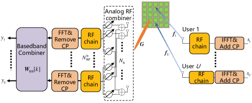
(a)

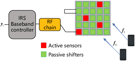
(b)

Figure 1: IRS aided communication models. (a) The Passive IRS aided hybrid architecture communication model. (b) The hybrid passive and active IRS aided communication model.

The passive IRS is installed with $N_{\mathsf{i}}$ passive phase shifters to provide a LoS link between the BS and the UEs. Each shifter in the IRS combines and reflects all the signals by dynamically adjusting the phase. During the $t^{\mathsf{th}}(t=1,2\ldots,T)$ pilot symbol, each shifter applies a new phase instantaneously without loss of generality. Thus the phase shift matrix of each IRS element in $t^{\mathsf{th}}$ symbol is denoted by

$$\boldsymbol{r}^{\left(t\right)}=\left[\beta^{\left(t\right)}e^{j\varphi_{1}^{(t)}},\beta^{\left(t\right)}e^{j\varphi_{2}^{(t)}},\ldots,\beta^{\left(t\right)}e^{j\varphi_{N_{\mathsf{i}}}^{(t)}}\right]^{\mathsf{T}}\in\mathbb{C}^{N_{\mathsf{i}}},$$ (1)

where $\beta^{\left(t\right)}\in\left[0,1\right]$ denotes the amplitude of the $n_{\mathsf{i}}^{\mathsf{th}}$ $(n_{\mathsf{i}}=1,2\ldots,N_{\mathsf{i}})$ IRS shifter, and $\varphi_{n_{\mathsf{i}}}^{(t)}\in\left[0,2\pi\right]$ is the corresponding phase. The BS first combines the received signals with an analog combiner $\boldsymbol{W}_{\mathsf{RF}}^{(t)}\in\mathbb{C}^{N_{\mathsf{b}}\times N_{\mathsf{RF}}^{\mathsf{b}}}$ where $N_{\mathsf{s}}=N_{\mathsf{RF}}^{\mathsf{b}}$ denotes data streams from BS to UEs. Then, the signals are transformed into the frequency-domain using $N_{\mathsf{RF}}^{\mathsf{b}}$ parallel $K$-point fast fourier transform and combined with digital baseband combiner $\boldsymbol{W}_{\mathsf{BB}}^{(t)}[k]\in\mathbb{C}^{N_{\mathsf{RF}}^{\mathsf{b}}\times N_{\mathsf{s}}}$. During the $t^{\mathsf{th}}$ transmission symbol, the $k^{\mathsf{th}}$ subcarrier received signals $\boldsymbol{y}^{\left(t\right)}[k]\in\mathbb{C}^{N_{\mathsf{s}}\times 1}$ is modeled by

$$\boldsymbol{y}^{\left(t\right)}[k]=\boldsymbol{W}_{\mathsf{b}}^{\left(t\right)}[k]^{\mathsf{H}}\sum_{u=1}^{U}\boldsymbol{H}_{u}^{(t)}[k]s_{u}^{\left(t\right)}[k]+\boldsymbol{W}_{\mathsf{b}}^{\left(t\right)}[k]^{\mathsf{H}}\boldsymbol{n}^{(t)}[k],$$ (2)

where $\boldsymbol{W}_{\mathsf{b}}^{\left(t\right)}[k]=\boldsymbol{W}_{\mathsf{RF}}^{\left(t\right)}[k]\boldsymbol{W}_{\mathsf{BB}}^{(t)}$ denotes the hybrid combiner and $\boldsymbol{n}^{(t)}[k]\sim\mathcal{N}_{\mathbb{C}}\left(0,\sigma^{2}\mathbf{I}\right)$ is the additive white Gaussian noise with covariance $\sigma^{2}$ at the BS side; $s_{u}^{\left(t\right)}[k]$ denotes the transmitted pilot symbol subject to $\mathbb{E}\left[s_{u}^{\left(t\right)}[k]s_{u}^{\left(t\right)}[k]^{\mathsf{H}}\right]=1$. For simplicity, we assume that the direct link is blocked due to adverse propagation conditions [6]. The $\boldsymbol{H}_{u}^{\left(t\right)}[k]$ represents the effective frequency-domain channel response from the $u^{\mathsf{th}}$ user to the BS at the $k^{\mathsf{th}}$ subcarrier, which is equivalently written by

$$\boldsymbol{H}_{u}^{\left(t\right)}[k]=\boldsymbol{G}[k]\left(\mathcal{\mathsf{diag}}\left(\boldsymbol{r}^{\left(t\right)}\right)\boldsymbol{f}_{u}[k]\right),$$ (3)

where $\boldsymbol{G}[k]\in\mathbb{C}^{N_{\mathsf{b}}\times N_{\mathsf{i}}}$ and $\boldsymbol{f}_{u}[k]\in\mathbb{C}^{N_{\mathsf{i}}\times 1}$ stand for the reflected channel between BS and IRS and the direct channel between IRS and $u^{\mathsf{th}}$ user, respectively. Moreover, the UEs-IRS-BS cascaded channel can be modeled as

$$\boldsymbol{H}_{\mathsf{c},u}[k]=\boldsymbol{G}[k]\mathcal{\mathsf{diag}}\left(\boldsymbol{f}_{u}[k]\right).$$ (4)

II-B Hybrid IRS Aided MU-MISO System

The pilot overhead of cascaded UEs-IRS-BS estimation is proportional to the product of the number of IRS shifters and BS antennas, which yields extremely huge estimation time at the BS side. On the other hand, the performance gain of passive IRS is fundamentally limited by the severe multiplicative path loss of the cascaded channel [9]. To overcome the above drawbacks, a hybrid IRS architecture is developed in [22] and [14], as shown in Fig. 1 (b), which is composed of passive shifters and active sensors. Furthermore, $N_{\mathsf{i}}^{a}$ active sensors consist of both estimation and reflection phases. Considering the cost of high power consumption and hardware constraints, the active sensors connect to the baseband unit via an RF chain and directly sense the dynamic UEs-IRS channels by observing the received pilots in the estimation phase [14]. During the data transmission phase, the passive shifters and active sensors reflect the signals wave simultaneously. In a hybrid IRS system, we focus on the mobile UEs-IRS channel, where the received signals at the $t_{\mathsf{i}}^{\mathsf{th}}(t=1,\ldots,T_{\mathsf{i}})$ training symbol can be expressed as [23]

$$\boldsymbol{y}_{\mathsf{i}}^{\left(t_{\mathsf{i}}\right)}[k]=\boldsymbol{w}_{\mathsf{i}}^{\left(t_{\mathsf{i}}\right)}[k]^{\mathsf{H}}\sum_{u=1}^{U}\boldsymbol{f}_{u}[k]s_{u}^{\left(t_{\mathsf{i}}\right)}[k]+\boldsymbol{W}_{\mathsf{i}}^{\left(t_{\mathsf{i}}\right)}[k]^{\mathsf{H}}\boldsymbol{n}^{\left(t_{i}\right)}[k],$$ (5)

where $\boldsymbol{w}_{\mathsf{i}}\in\mathbb{C}^{N_{\mathsf{i}}\times 1}$ stacks a one-hot vector, with 0 indicating a passive shifter and 1 representing an active sensor.

III Channel Model and Problem Formulation

In this section, the channel model of the UEs-IRS and IRS-BS channels are first introduced. Then, we formulate the cascaded and UEs-IRS channel estimation problems as two sparse signal recovery problems in the frequency-domain.

III-A IRS Aided MISO Channel Model

1. Channel model) As mentioned above, the passive IRS aided channel is split into two subchannels. Without loss of generality, both $\boldsymbol{f}_{u}[k]$ and $\boldsymbol{G}[k]$ are presented by the geometric channel model [5]. Also, the channel matrix $\boldsymbol{f}_{d,u}$ ($\boldsymbol{G}_{d}$) is assumed to be frequency-selective, which is non-zero only for $d=1,\cdot\cdot\cdot,L_{\mathsf{c,f}}$ $\left(d=1,\cdot\cdot\cdot,L_{\mathsf{c,g}}\right)$ taps. We assume that BS is equipped with Uniform Linear Arrays (ULAs) and the IRS employs the $N_{\mathsf{i}}\left(N_{\mathsf{i}}=N_{\mathsf{i,x}}\times N_{\mathsf{i,y}}\right)$ uniform planar array (UPA). According to [24], the discrete delay-domain channels of $d^{\mathsf{th}}$ delay tap are given as

$$\boldsymbol{f}_{d,u}=\sqrt{\frac{N_{\mathsf{i}}}{L_{\mathsf{p,f}}}}\sum_{l=1}^{L_{\mathsf{p,f}}}\alpha_{l,u}p(dT_{\mathsf{s}}-\tau_{l,u})\boldsymbol{a}_{\mathsf{i}}(\theta_{\mathsf{i},l,u}^{\mathsf{A}},\varphi_{\mathsf{i},l,u}^{\mathsf{A}}),$$ (6)

$$\boldsymbol{G}_{d}=\sqrt{\frac{N_{\mathsf{i}}N_{\mathsf{b}}}{L_{\mathsf{p,g}}}}\sum_{l=1}^{L_{\mathsf{p,g}}}\beta_{l}p(dT_{\mathsf{s}}-\tau_{l})\boldsymbol{a}_{\mathsf{b}}(\theta_{\mathsf{b},l}^{\mathsf{A}})\boldsymbol{a}_{\mathsf{i}}^{\mathsf{H}}(\theta_{\mathsf{i},l}^{\mathsf{D}},\varphi_{\mathsf{i},l}^{\mathsf{D}}),$$ (7)

for the $u^{\mathsf{th}}$ user, $\alpha_{l,u}$ ($\beta_{l}$) and $\tau_{l,u}$ denote propagation gain of the UEs-IRS (IRS-BS) channel and delay corresponding to $l^{\mathsf{th}}$ path. $L_{\mathsf{p,f}}$ and $L_{\mathsf{p,g}}$ represent the number of $\boldsymbol{f}_{d,u}$ and $\boldsymbol{G}_{d}$ paths, respectively. For simplicity, we assume that the number of propagation paths for different UEs remains constant; $p(\tau)$ is the pulse-shaping filter evaluated at $\tau$ and $T_{s}$ denotes the sampling period; $\theta_{\mathsf{i},l,u}^{\mathsf{A}}$ ($\varphi_{\mathsf{i},l,u}^{\mathsf{A}}$) and $\theta_{\mathsf{i},l}^{\mathsf{D}}$ ($\varphi_{\mathsf{i},l}^{\mathsf{D}}$) represent azimuth (elevation) angle of arrival (AoA) and angle of departure (AoD) of the $l^{\mathsf{th}}$ path at the IRS, respectively. $\theta_{\mathsf{b},l}^{\mathsf{A}}$ is the AoA of the $l^{\mathsf{th}}$ path at BS side. The array steering vectors of the BS and the IRS are denoted by $\boldsymbol{a}_{\mathsf{b}}\in\mathbb{C}^{N_{\mathsf{b}}\times 1}$ and $\boldsymbol{a}_{\mathsf{i}}\in\mathbb{C}^{N_{\mathsf{i}}\times 1}$, respectively. Thus the normalized array response vectors are expressed as

$$\boldsymbol{a}_{\mathsf{b}}(\theta)=\frac{1}{\sqrt{N_{\mathsf{b}}}}\left[1\cdots e^{\frac{j2\pi d_{\mathsf{s}}}{\lambda_{\mathsf{c}}}(n_{\mathsf{b}}-1)\sin(\theta)}\cdots e^{\frac{j2\pi d_{\mathsf{s}}}{\lambda_{\mathsf{c}}}(N_{\mathsf{b}}-1)\sin(\theta)}\right]_{,}^{\mathsf{T}}$$ (8)

$$\boldsymbol{a}_{\mathsf{i}}(\theta,\varphi)=\frac{1}{\sqrt{N_{\mathsf{i}}}}\left[1\cdots e^{\frac{j2\pi d_{\mathsf{s}}}{\lambda_{\mathsf{c}}}\left((n_{\mathsf{1}}-1)\sin(\theta)\cos(\varphi)+(n_{\mathsf{2}}-1)\sin(\varphi)\right)}\cdots e^{\frac{j2\pi d_{\mathsf{s}}}{\lambda_{\mathsf{c}}}\left((N_{\mathsf{i,x}}-1)\sin(\theta)\cos(\varphi)+(N_{\mathsf{i,y}}-1)\sin(\varphi)\right)}\right],$$ (9)

where $d_{\mathsf{s}}$ and $\lambda_{\mathsf{c}}$ are the antenna adjacent spacing and carrier wavelength, respectively, and we set $d_{\mathsf{s}}/\lambda_{\mathsf{c}}=1/2$ without loss of generality. During the estimating phase, both the BS and the user are considered to know the array response vectors and IRS phase-shift matrices. Thus, the channel can be reformulated more compactly as $\boldsymbol{f}_{d,u}=\boldsymbol{\boldsymbol{A}}_{\mathsf{R,i},u}\Delta_{\mathsf{f},d,u}\boldsymbol{a}_{\mathsf{T},u}^{\mathsf{H}}$, where $\Delta_{\mathsf{f},d,u}\in\mathbb{C}^{L_{\mathsf{p,f}}\times L_{\mathsf{p,f}}}$ is diagonal with non-zero entries $\alpha_{l,u}p(dT_{\mathsf{s}}-\tau_{l,u})$, which can be written as

$$\Delta_{\mathsf{f},d,u}=\sqrt{\frac{N_{\mathsf{i}}}{L_{\mathsf{p,f}}}}\mathcal{\mathsf{diag}}\left(\alpha_{1,u}p(dT_{\mathsf{s}}-\tau_{1,u}),\ldots,\cdots\alpha_{L_{\mathsf{p,f}},u}p(dT_{\mathsf{s}}-\tau_{L_{\mathsf{p,f}},u})\right),$$ (10)

where $\boldsymbol{\boldsymbol{A}}_{\mathsf{R,i},u}=\left[\boldsymbol{a}_{\mathsf{i}}(\theta_{\mathsf{i},1,u}^{\mathsf{A}},\varphi_{\mathsf{i},1,u}^{\mathsf{A}}),\ldots\boldsymbol{a}_{\mathsf{i}}(\theta_{\mathsf{i},L_{\mathsf{p,f}},u}^{\mathsf{A}},\varphi_{\mathsf{i},L_{\mathsf{p,f}},u}^{\mathsf{A}}),\right]\in\mathbb{C}^{N_{\mathsf{i}}\times L_{\mathsf{p,f}}}$ and $\boldsymbol{a}_{\mathsf{T},u}=\left[\theta_{1,u}^{\mathsf{D}},\ldots,\theta_{L_{\mathsf{p,f}},u}^{\mathsf{D}}\right]\in\mathbb{C}^{1\times L_{\mathsf{p,f}}}$ denote the array steering vectors of AoAs at IRS and AoD at the $u^{\mathsf{th}}$ user side, respectively. Using (6) and (7), the frequency-domain complex channel at subcarrier $k$ can be denoted as

$$\boldsymbol{f}_{u}\mathit{\left[k\right]}=\sum_{d=1}^{L_{\mathsf{c,f}}}\boldsymbol{F}_{d,u}e^{-j\frac{2\pi dk}{K}}=\boldsymbol{\boldsymbol{A}}_{\mathsf{R,i},u}\mathsf{\text{$\mathbf{\Delta}_{\mathsf{f},u}$}\left[k\right]}\boldsymbol{a}_{\mathsf{T},u}^{\mathsf{H}},$$ (11)

$$\boldsymbol{G}\left[k\right]=\sum_{d=1}^{L_{\mathsf{c,g}}}\boldsymbol{G}_{d}e^{-j\frac{2\pi dk}{K}}=\boldsymbol{A}_{\mathsf{R,b}}\mathsf{\text{\text{$\mathbf{\Delta}_{\mathsf{g}}$}}\mathit{\left[k\right]}}\boldsymbol{A}_{\mathsf{T,i}}^{\mathsf{H}},$$ (12)

where $\text{$\mathbf{\Delta}_{\mathsf{f},u}$}\mathit{\left[k\right]}\in\mathbb{C}^{L_{\mathsf{c,f}}\times L_{\mathsf{c,f}}}$ and $\text{$\mathbf{\Delta}_{\mathsf{g}}$}\mathit{\left[k\right]}\in\mathbb{C}^{L_{\mathsf{c,g}}\times L_{\mathsf{c,g}}}$ are diagonal with non-zero complex entries such that $\text{$\mathbf{\Delta}_{\mathsf{f},u}$}\mathit{\left[k\right]}=$$\Sigma_{d=1}^{L_{\mathsf{c,f}}}\Delta_{\mathsf{f},d,u}e^{-j\frac{2\pi dk}{K}}$ and $\text{\text{$\mathbf{\Delta}_{\mathsf{g}}$}}\mathit{\left[k\right]}=\Sigma_{d=1}^{L_{\mathsf{c,g}}}\Delta_{\mathsf{g},d}e^{-j\frac{2\pi dk}{K}}$, $k=1,2,\cdots K$.

2. Virtual channel model extention) The training overhead of cascaded channel estimation is proportional to the number of BS, IRS and user antennas. Fortunately, due to the angular sparsity of the mmWave channel, we can formulate the cascaded channel estimation as a sparse recovery problem [23] and adopt CS methods to reduce pilot overhead. To mitigate the power leakage effect in the angle domain, we further approximate the $\boldsymbol{f}_{u}\mathit{\left[k\right]}$ by designing redundant dictionary matrices with higher angular resolution. The extended $\boldsymbol{f}_{u}\mathit{\left[k\right]}$ and $\boldsymbol{G}\mathit{\left[k\right]}$ in (11) and (12) are rewritten as

$$\boldsymbol{f}_{u}\mathit{\left[k\right]}=\widetilde{\boldsymbol{A}}_{\mathsf{R,i},u}\mathsf{\text{$\mathbf{\widetilde{\Delta}}_{\mathsf{f},u}$}\left[k\right]}\boldsymbol{\widetilde{a}}_{\mathsf{T},u}^{\mathsf{H}},$$ (13)

$$\boldsymbol{G}\mathit{\left[k\right]}=\boldsymbol{\widetilde{A}}_{\mathsf{R,b}}\mathsf{\text{$\mathbf{\widetilde{\Delta}}_{\mathsf{g}}$}\mathit{\left[k\right]}}\boldsymbol{\widetilde{A}}_{\mathsf{T,i}}^{\mathsf{H}},$$ (14)

where $\text{$\mathbf{\widetilde{\Delta}}_{\mathsf{f},u}$}\left[k\right]\in\mathbb{C}^{G_{\mathsf{i}}\times G_{\mathsf{u}}}$ and $\text{$\mathbf{\widetilde{\Delta}}_{\mathsf{g}}$}\mathit{\left[k\right]}\in\mathbb{C}^{G_{\mathsf{b}}\times G_{\mathsf{i}}}$ correspond to complex virtual angular-domain channels. The dictionary matrices $\boldsymbol{\widetilde{a}}_{\mathsf{T},u}\in\mathbb{C}^{1\times G_{\mathsf{u}}}$ ($\boldsymbol{\widetilde{A}}_{\mathsf{T,i}}\in\mathbb{C}^{N_{\mathsf{i}}\times G_{\mathsf{i}}}$) and $\boldsymbol{\widetilde{A}}_{\mathsf{R,i},u}\in\mathbb{C}^{N_{\mathsf{i}}\times G_{\mathsf{i}}}$ ($\boldsymbol{\widetilde{A}}_{\mathsf{R,b}}\in\mathbb{C}^{N_{\mathsf{b}}\times G_{\mathsf{b}}}$) contain the UE (IRS) and IRS (BS) array response vectors evaluated on a grid of size $G_{\mathsf{u}}$ ($G_{\mathsf{i}}$) and $G_{\mathsf{i}}$ ($G_{\mathsf{b}}$) for the AoD and AoA, i.e., $\boldsymbol{\widetilde{a}}_{\mathsf{T},u}=\left[\theta_{u,1}^{\mathsf{D}},\ldots,\theta_{u,G_{\mathsf{u}}}^{\mathsf{D}}\right]$ and $\qquad\boldsymbol{\boldsymbol{\widetilde{A}}}_{\mathsf{R,i},u}=\left[\boldsymbol{a}_{\mathsf{i}}(\theta_{\mathsf{i},1,u}^{\mathsf{A}},\varphi_{\mathsf{i},1,u}^{\mathsf{A}}),\ldots\boldsymbol{a}_{\mathsf{i}}(\theta_{\mathsf{i},G_{\mathsf{i}},u}^{\mathsf{A}},\varphi_{\mathsf{i},G_{\mathsf{i}},u}^{\mathsf{A}})\right]$, respectively. Due to the few number of scattering paths, we assume that the grid of AoAs and AoDs of IRS have the same size $G_{\mathsf{i}}$.

III-B Problem Formulation

We assume that $U$ UEs use mutually orthogonal pilot signals [25], the pilot signals of each user can be distinguished and processed separately. Accordingly, by stacking $K$ UEs’ quantities, the received signals of the $t^{\mathsf{th}}$ training symbol in (2) can be rewritten as

$$\boldsymbol{y}^{\left(t\right)}[k]=\boldsymbol{W}_{\mathsf{b}}^{\left(t\right)}[k]^{\mathsf{H}}\boldsymbol{H}^{(t)}[k]s^{\left(t\right)}[k]+\boldsymbol{n}_{\mathsf{c}}^{(t)}[k],$$ (15)

where $\boldsymbol{n}_{\mathsf{c}}^{(t)}[k]=\boldsymbol{W}_{\mathsf{b}}^{\left(t\right)}[k]^{\mathsf{H}}\boldsymbol{n}^{(t)}[k]$ is the combined noise vector received at the $k^{\mathsf{th}}$ subcarrier.

1) Cascaded channel with passive IRS: In the $t^{\mathsf{th}}$ symbol training phase, the pilot symbol $s^{\left(t\right)}$ is known at the receiver, and BS adopts the training combiner $\boldsymbol{W}_{\mathsf{b}}^{\left(t\right)}$. Moreover, $s^{\left(t\right)}$, $\boldsymbol{W}_{\mathsf{b}}^{\left(t\right)}$ and $\boldsymbol{n}_{\mathsf{c}}^{(t)}$ are considered to be frequency-flat to reduce the complexity of estimation [11, 24]. Each entry in $\boldsymbol{W}_{\mathsf{b}}$ is normalized so that their square modules are $\frac{1}{N_{\mathsf{b}}}$. We assume that $\boldsymbol{f}\mathit{\left[k\right]}$ and $\boldsymbol{G}\left[k\right]$ are invariant for several consecutive symbols, and the frame duration is shorter than the channel coherence time [24]. Exploiting the equality $\mathsf{vec}\left(\boldsymbol{AXB}\right)=\left(\boldsymbol{B}^{\mathsf{T}}\otimes\boldsymbol{A}\right)\mathsf{vec}\left(\boldsymbol{X}\right)$, the received signals can be rewritten as

$$\boldsymbol{y}^{\left(t\right)}[k]=\left(s^{\left(t\right)\mathsf{T}}\otimes\boldsymbol{W}_{\mathsf{b}}^{(t)\mathsf{H}}\right)\mathsf{vec}\left(\boldsymbol{H}^{\left(t\right)}[k]\right)+\boldsymbol{n}_{\mathsf{c}}^{(t)}.$$ (16)

Combining (13) and (14) with (3), the vectorization of $\boldsymbol{H}^{\left(t\right)}[k]$ can be expressed as

$$\mathsf{vec}\left(\boldsymbol{H}^{\left(t\right)}[k]\right)$$

$$=\mathsf{vec}\left(\boldsymbol{\widetilde{A}}_{\mathsf{R,b}}\widetilde{\boldsymbol{\Delta}}_{\mathsf{g}}\mathit{\left[k\right]}\boldsymbol{\widetilde{A}}_{\mathsf{T,i}}^{\mathsf{H}}\mathrm{diag}\left(\boldsymbol{r}^{\left(t\right)}\right)\boldsymbol{\widetilde{A}}_{\mathsf{R,i}}\mathsf{\mathsf{\text{$\mathbf{\widetilde{\Delta}}_{\mathsf{f}}$}\left[k\right]}}\boldsymbol{\widetilde{a}}_{\mathsf{T}}^{\mathsf{H}}\right)$$

$$\overset{\left(a\right)}{=}\left(\boldsymbol{\widetilde{a}}_{\mathsf{T}}^{\mathsf{*}}\varotimes\boldsymbol{\widetilde{A}}_{\mathsf{R,b}}\right)\left(\boldsymbol{\widetilde{\Delta}}_{\mathsf{f}}^{\mathsf{T}}\mathit{\left[k\right]}\varotimes\widetilde{\boldsymbol{\Delta}}_{\mathsf{g}}\mathit{\left[k\right]}\right)\mathsf{vec}\left(\boldsymbol{\widetilde{A}}_{\mathsf{T,i}}^{\mathsf{H}}\mathrm{d}\left(\boldsymbol{r}^{\left(t\right)}\right)\boldsymbol{\widetilde{A}}_{\mathsf{R,i}}\right)$$

$$\overset{\left(b\right)}{=}\left(\boldsymbol{\widetilde{a}}_{\mathsf{T}}^{\mathsf{*}}\varotimes\boldsymbol{\widetilde{A}}_{\mathsf{R,b}}\right)\left(\boldsymbol{\widetilde{\Delta}}_{\mathsf{f}}^{\mathsf{T}}\mathit{\left[k\right]}\varotimes\widetilde{\boldsymbol{\Delta}}_{\mathsf{g}}\mathit{\left[k\right]}\right)\boldsymbol{D}\boldsymbol{r}^{\left(t\right)}$$

$$\overset{\left(c\right)}{=}\left(D_{\mathsf{g}}^{\mathsf{T}}\otimes\left(\boldsymbol{\widetilde{a}}_{\mathsf{T}}^{\mathsf{*}}\varotimes\boldsymbol{\widetilde{A}}_{\mathsf{R,b}}\right)\right)\widetilde{\boldsymbol{X}}\mathit{\left[k\right]}\boldsymbol{r}^{\left(t\right)},$$ (17)

where in $(a)$, $\left(\boldsymbol{\widetilde{\Delta}}_{\mathsf{f}}^{\mathsf{T}}\mathit{\left[k\right]}\varotimes\widetilde{\boldsymbol{\Delta}}_{\mathsf{g}}\mathit{\left[k\right]}\right)\in\mathbb{C}^{G_{\mathsf{u}}G_{\mathsf{b}}\times G_{\mathsf{i}}^{\mathsf{2}}}$ is a sparse vector of the virtual angular-domain channels with $L_{\mathsf{p,f}}L_{\mathsf{p,g}}$ non-zero elements, $(b)$ follows from the property $\mathsf{vec}(ABC)=(C^{\mathsf{T}}\odot A)b$, where $b$ denotes the diagonal element vector of a diagonal matrix and $\boldsymbol{D}\overset{\Delta}{=}\left(\boldsymbol{\widetilde{A}}_{\mathsf{R,i}}^{\mathsf{T}}\varodot\boldsymbol{\widetilde{A}}_{\mathsf{T,i}}^{\mathsf{H}}\right)\in\mathbb{C}^{G_{\mathsf{i}}^{\mathsf{2}}\times N_{\mathsf{i}}}$ is a sparse matrix. $(c)$ follows the guidance of [6], $\boldsymbol{D}$ can be further simplified. Specifically, the matrix $\boldsymbol{D}$ only contains $G_{\mathsf{i}}$ distinct rows, which are the first $G_{\mathsf{i}}$ rows of $\boldsymbol{D}$, i.e., $\boldsymbol{D}_{\mathsf{g}}\overset{\Delta}{=}\boldsymbol{D}(0:G_{\mathsf{i}}-1,:)$. In addition, we define $\widetilde{\boldsymbol{X}}\mathit{\left[k\right]\in\mathbb{C}^{G_{\mathsf{u}}G_{\mathsf{b}}\times G_{\mathsf{i}}}}$ is a merged version of $\boldsymbol{Q}\overset{\Delta}{=}\boldsymbol{\widetilde{\Delta}}_{\mathsf{f}}^{\mathsf{T}}\mathit{\left[k\right]}\varotimes\widetilde{\boldsymbol{\Delta}}_{\mathsf{g}}\mathit{\left[k\right]}$, i.e., $\widetilde{\boldsymbol{X}}\mathit{\left[k\right]}(:,i)=\sum_{j\epsilon M_{i}}\boldsymbol{Q}(:,j)$, where $M_{i}$ is the set of indices corresponding to these rows in $\boldsymbol{D}$. Leveraging these properties, the $\boldsymbol{y}^{\left(t\right)}[k]$ in (16) can be further represented as

$$\boldsymbol{y}^{\left(t\right)}[k] =\left(\boldsymbol{r}^{\left(t\right)\mathsf{T}}\otimes\left(s^{\left(t\right)\mathsf{T}}\otimes\boldsymbol{W}_{\mathsf{b}}^{(t)\mathsf{H}}\right)\right)\boldsymbol{\Psi}\boldsymbol{x}\mathit{\left[k\right]}+\boldsymbol{n}_{\mathsf{c}}^{(t)}[k]$$

$$=\boldsymbol{\Phi}^{(t)}\boldsymbol{\Psi}\boldsymbol{x}\mathit{\left[k\right]}+\boldsymbol{n}_{\mathsf{c}}^{(t)}[k],$$ (18)

where $\boldsymbol{\Psi}\overset{\Delta}{=}\boldsymbol{D}_{\mathsf{g}}^{\mathsf{T}}\varotimes\left(\boldsymbol{\widetilde{a}}_{\mathsf{T}}^{\mathsf{*}}\varotimes\boldsymbol{\widetilde{A}}_{\mathsf{R,b}}\right)\in\mathbb{C}^{N_{\mathsf{i}}N_{\mathsf{b}}\times G_{\mathsf{i}}G_{\mathsf{b}}G_{\mathsf{u}}}$ is the redundant dictionary of the cascaded channel; $\boldsymbol{\Phi}^{(t)}\overset{\Delta}{=}\left(\boldsymbol{r}^{\left(t\right)T}\otimes\left(s^{\left(t\right)\mathsf{T}}\otimes\boldsymbol{W}_{\mathsf{b}}^{(t)\mathsf{H}}\right)\right)$ denotes the measurement matrix and $\boldsymbol{x}\mathit{\left[k\right]}=\mathsf{vec}\left(\widetilde{\boldsymbol{X}}\mathit{\left[k\right]}\right)\in\mathbb{C}^{G_{\mathsf{u}}G_{\mathsf{b}}G_{\mathsf{i}}}$ is the sparse vector of the cascaded channel. By stacking $T$ successive received pilots, we obtain the system model in the virtual angular-domain as

$$\boldsymbol{y}[k]=\boldsymbol{\Phi\Psi}\boldsymbol{x}\mathit{\left[k\right]}+\boldsymbol{n}_{\mathsf{c}}[k],$$ (19)

where $\boldsymbol{y}\left[k\right]=\left[\boldsymbol{y}^{\left(1\right)}[k],\cdots,\boldsymbol{y}^{\left(T\right)}[k]\right]^{\mathsf{T}}\in\mathbb{C}^{M\times 1}$ ($M=T\times N_{\mathsf{s}}$), $\boldsymbol{\Phi}=\left[\boldsymbol{\Phi}^{\left(1\right)},\cdots,\boldsymbol{\Phi}^{\left(T\right)}\right]^{\mathsf{T}}\in\mathbb{C}^{M\times N_{\mathsf{i}}N_{\mathsf{b}}}$ and $\boldsymbol{n}_{\mathsf{c}}[k]=\left[\boldsymbol{n}_{\mathsf{c}}^{\left(1\right)}[k],\cdots,\boldsymbol{n}_{\mathsf{c}}^{\left(T\right)}[k]\right]^{\mathsf{T}}$ of size $M\times 1$. By stacking $K$ subcarriers quantities from $\boldsymbol{y}[k]$, the vector $\boldsymbol{x}[k]$ in (19) can be considered as a typical multiple-measurement-vectors (MMV) sparse reconstruction problem, i.e.,

$$\mathsf{min}\left(\sum_{k=1}^{K}\left\|\boldsymbol{x}[k]\right\|_{1}\right),\quad\mathsf{s.t.}\left\|\boldsymbol{Y}-\boldsymbol{\Phi\Psi}\left(\boldsymbol{X}\right)\right\|_{2}^{2}<\varepsilon,$$ (20)

where $\boldsymbol{Y}=\left[\boldsymbol{y}[1],\cdots,\boldsymbol{y}[K]\right]\in\mathbb{C}^{M\times K}$, $\boldsymbol{X}\in\mathbb{C}^{G_{\mathsf{i}}G_{\mathsf{b}}G_{\mathsf{u}}\times K}$ and $\varepsilon$ is error tolerance.

2) Channel with hybrid IRS: From the discussion in Section II-B, the active elements receive orthogonal pilots and estimate the UEs-IRS channel vectors. By leveraging tools from CS and extending to $T_{\mathsf{i}}$ received signals, the uplink signals at the IRS side can be formulated as

$$\boldsymbol{y}_{\mathsf{i}}[k]=\boldsymbol{\Phi}_{\mathsf{i}}\mathsf{vec}\left(\boldsymbol{\widetilde{A}}_{\mathsf{R,i}}\mathsf{\mathsf{\text{$\mathbf{\widetilde{\Delta}}_{\mathsf{i,f}}$}}}\left[k\right]\boldsymbol{\widetilde{a}}_{\mathsf{T}}^{\mathsf{H}}\right)+\boldsymbol{n}_{\mathsf{i}}[k]=\boldsymbol{\Phi}_{\mathsf{i}}\boldsymbol{\Psi}_{\mathsf{i}}\left(\boldsymbol{x}_{\mathsf{i}}[k]\right)+\boldsymbol{n}_{\mathsf{i}}[k]\text{.}$$ (21)

According to (18) and (19), $\boldsymbol{\Phi}_{\mathsf{i}}=s^{\mathsf{T}}\otimes\boldsymbol{w}_{\mathsf{i}}^{\mathsf{H}}\in\mathbb{C}^{T_{\mathsf{i}}\times N_{\mathsf{i}}}$ and $\boldsymbol{\Psi}_{\mathsf{i}}=\mathsf{vec}\left(\boldsymbol{\widetilde{a}}_{\mathsf{T}}^{\mathsf{*}}\varotimes\boldsymbol{\widetilde{A}}_{\mathsf{R,i}}\right)\in\mathbb{C}^{N_{\mathsf{i}}\times G_{\mathsf{u}}G_{\mathsf{i}}}$ denote the IRS reflecting measurement matrix and the redundant dictionary of the UE-IRS channel, respectively. $\boldsymbol{n}_{\mathsf{i}}^{(t)}[k]$ is stacked noise vector of $k^{\mathsf{th}}$ subcarrier at the IRS side and $\boldsymbol{x}_{\mathsf{i}}[k]=\mathsf{vec}\left(\mathsf{\mathsf{\text{$\mathbf{\widetilde{\Delta}}_{\mathsf{i,f}}$}}}\left[k\right]\right)$ represents the vectorization operation on the sparse vector of the UE-IRS channel. We assume that the active elements are randomly selected from the IRS reflectors [26]. For simplicity, we employ $G_{\mathsf{u}}=1$ in this work.

There are various algorithms to solve sparse reconstruction MMV problem. For example, the simultaneous weighted orthogonal matching pursuit (SWOMP) algorithm [11], vector AMP (VAMP) technique [27] and LAMP algorithm [17, 21] neglect the sparse structure of the sparse channel matrix and directly vectorize $\boldsymbol{y}^{\left(t\right)}[k]$ and the sparse channel matrix into vectors, which lead these CS algorithms failing to achieve satisfactory accuracy in the IRS channels [8]. Meanwhile, some single measurement vector (SMV) [11] and MMV [28] algorithms assume that the channel has the same sparse structure for all subcarriers, which ignores the information in the frequency-domain and degrades the recovery performance [22]. Therefore, these approaches motivate us to develop a channel estimator for the IRS aided system by leveraging both sparse structure and frequency properties.

IV Proposed Hybrid Driven Networks for Channel Estimation

Inspired by data driven and model driven networks, this section proposes an attention network aided RLAMP network to solve the sparse channel estimation problem. The network adopts a denoising convolution neural network (DnCNN) to remove signal noise from the received signals. By utilizing the higher resolution dictionary matrix, the attention network extracts spatial information in the sparse channel and frequency characteristics between different subcarriers. Next, the network structures and training details of will be elaborated sequentially.

IV-A Model Driven: Overview of the RLAMP Based Estimation Approach

We integrate the LAMP network and the residual learning [29] to the proposed networks. Before explicit estimation, the RLAMP network requires to calculate the atom, which is defined as the vector in the measurement matrix [11]. The complex correlation vector $\boldsymbol{C}\in\mathbb{C}^{G_{\mathsf{i}}G_{\mathsf{b}}\times K}$ is defined as

$$\left[\begin{array}[]{c}\mathsf{Re}\left(\boldsymbol{\boldsymbol{C}}\right)\\ \mathsf{Im}\left(\boldsymbol{C}\right)\end{array}\right]=\left[\begin{array}[]{c}\mathsf{Re}\left(\boldsymbol{\beta}_{1}\right)\\ \mathsf{Im}\left(\boldsymbol{\beta}_{1}\right)\end{array}\begin{array}[]{c}-\mathsf{Im}\left(\boldsymbol{\beta}_{1}\right)\\ \mathsf{Re}\left(\boldsymbol{\beta}_{1}\right)\end{array}\right]\left[\begin{array}[]{c}\mathsf{Re}\left(\boldsymbol{Y}\right)\\ \mathsf{Im}\left(\boldsymbol{Y}\right)\end{array}\right],$$ (22)

where $\boldsymbol{\beta}_{1}$ is a trainable matrix with the same size as matrix $\text{$\boldsymbol{\Upsilon}$}^{\mathsf{H}}$, where $\boldsymbol{\boldsymbol{\Upsilon}}=\boldsymbol{\Phi\Psi}\in\mathbb{C}^{M\times G_{\mathsf{i}}G_{\mathsf{b}}}$ represents the equivalent measurement matrix. As Fig. 2 shows, the MMV-RLAMP extends the trainable parameters into the iteration of the traditional AMP algorithms, which adaptively learn and optimize the network from the channel samples. In LAMP [30], the input and output are typically limited to vectors, while the received signals, measurement and estimated channel are matrices. Therefore, the inputs and outputs at each iteration layer need to be vectorized. Specifically, $\boldsymbol{X}_{n}\in\mathbb{C}^{G_{\mathsf{i}}G_{\mathsf{b}}\times K}$ and $\boldsymbol{V}_{n}\in\mathbb{C}^{M\times K}$ are the output of the $n\mathsf{{}^{th}}$ layer ($n=1,\cdots N$). Following the guidance of the AMP algorithm, the estimated matrix $\boldsymbol{\widehat{X}}_{n}$ and residual matrix $\boldsymbol{V}_{n}$ of each iteration in the network are formulated as follows

$$\boldsymbol{\widehat{X}}_{n}=\eta\left(\boldsymbol{R}_{n};\boldsymbol{\lambda}_{\eta,n},\boldsymbol{\sigma}_{n}\right)+\boldsymbol{\widehat{X}}_{n-1},$$ (23)

$$\boldsymbol{V}_{n}=\boldsymbol{Y}-\boldsymbol{\Upsilon}\boldsymbol{\widehat{X}}_{n}+\boldsymbol{b}_{n}\boldsymbol{V}_{n-1},$$ (24)

where $\boldsymbol{R}_{1}=\boldsymbol{C}$, $\boldsymbol{V}_{0}=\boldsymbol{Y}$, $\boldsymbol{\widehat{X}}_{0}=0$, and

$$\boldsymbol{\sigma}_{n}=\frac{1}{\sqrt{M}}\left\|\boldsymbol{V}_{n-1}\right\|_{\mathsf{F}},$$ (25)

$$\boldsymbol{b}_{n}=\frac{\lambda_{\mathsf{b},n}}{\sqrt{M}}\sum_{j=1}^{G}\frac{\partial\left[\eta\left(\boldsymbol{R}_{n};\boldsymbol{\lambda}_{\eta,n},\boldsymbol{\sigma}_{n}^{\mathsf{2}}\right)\right]_{j}}{\partial\left[\boldsymbol{R}_{n}\left(j,:\right)\right]},$$ (26)

$$\boldsymbol{R}_{n+1}=\boldsymbol{\widehat{X}}_{n}+\boldsymbol{\beta}_{n+1}\boldsymbol{V}_{n},$$ (27)

with $G=G_{\mathsf{i}}G_{\mathsf{b}}$; the term $\boldsymbol{b}_{n}$ in (24) is the Onsager correction [17], which is derivative of $\eta(:,:)$ and accelerates the estimation convergence; and $\boldsymbol{\beta}_{n}\in\mathbb{C}^{G_{\mathsf{i}}G_{\mathsf{b}}\times M}$ is a linear parameter of the $n\mathsf{{}^{th}}$ layer. Equation (23) indicates residual learning mechanism. Specifically, $\boldsymbol{\widehat{X}}_{n-1}$ is directly added to the outputs of the $n\mathsf{{}^{th}}$ layer. This identity shortcut connection takes advantage of prior $n-1$ layers knowledge to further overcome the vanishing gradient problem and accelerate training progress without introducing additional parameters and computational complexity. The shrinkage function $\eta(:,:)$ in (26) replaces the nonlinear activation function in iteration, it can be expressed as

$$\left[\eta\left(\boldsymbol{R}_{n};\boldsymbol{\lambda}_{\eta,n},\boldsymbol{\sigma}_{n}^{\mathsf{2}}\right)\right]_{j}\overset{\Delta}{=}\lambda_{1\text{,}n}\mathsf{max}\left(\left|\boldsymbol{r}_{n,j}\right|-\lambda_{2,n}\boldsymbol{\sigma}_{n}\text{,0}\right)\mathsf{sgn}\text{($\boldsymbol{r}_{n,j}$)},$$ (28)

where $\boldsymbol{r}_{n,j}=\boldsymbol{R}_{n}(j,:)$ express $j^{\mathsf{th}}$ row of $\boldsymbol{R}_{n}$; and $\boldsymbol{\lambda}_{n}=\left\{\lambda_{1\text{,}n},\lambda_{2\text{,}n},\lambda_{\mathsf{b},n}\right\}\in\mathbb{R}^{3}$ is the predefined and nonlinear shrinkage parameter of the $n\mathsf{{}^{th}}$ layer and $\boldsymbol{\lambda}_{\eta,n}=\left\{\lambda_{1\text{,}n},\lambda_{2\text{,}n}\right\}\in\mathbb{R}^{2}$. The linear parameter $\boldsymbol{\beta}_{n}$ and nonlinear shrinkage parameter $\boldsymbol{\lambda}_{n}$ are regarded as trainable parameters, which are learned in each iteration from training data. Roughly speaking, our network adopts a soft-Threshold function rather than other denoiser such as denoising-based LAMP (LDAMP) [18] and Gaussian mixture LAMP (GM-LAMP) [20]. We propose a denoising network before the RLAMP, which learns and mitigates the noise component in the $\boldsymbol{x}[k]$, the details described in subsection IV-B.

Figure 2: The $n^{\mathsf{th}}$ layer structure of the DA-RLAMP network.

However, the MMV-LAMP networks for channel estimation suffer from the following problems: (i) The traditional LAMP network and its variants are applicable for any signal without considering the channel sparse structure; (ii) Some developed architectures focus on the design of denoiser (shrinkage function) [20, 31] to obtain residual noise vector in different iterations, which neglect the channel properties. To improve the estimation performance, we will propose an MMV-DA-RLAMP network based on a denoising network and the attention mechanism in the next subsection. The proposed network implicitly learns the sparse characteristics of signals without any channel prior information.

IV-B Data Driven: Channel Feature Filtering and Enhancement Via Denoising Network and Attention Mechanism

In Fig. 3, the denoising network consists of $L_{\mathsf{d}}$ denoising layers to learn the residual noise from the noisy correlation matrix $\boldsymbol{C}$. Since $\boldsymbol{\boldsymbol{\Upsilon}}$ is a complex-valued matrix, we divide the real part and imaginary part to facilitate feature extraction. Table I summarizes the hyperparameters of DnCNN and the attention network.

Table I: Hyperparameters of the DnCNN and Attention Network.

Input: Noisy correlation vector $\boldsymbol{C}_{\mathsf{a}}\in\mathbb{R}^{2\times G_{\mathsf{i}}\times G_{\mathsf{b}}\times K}$
Denoising Network
Layers	Operations	Filter Size
1~$L_{\mathsf{d}}-$1	Conv+Nonlinear	$K\times\left(3\times 3\times K\right)$
$L_{\mathsf{d}}$	Conv	$K\times\left(3\times 3\times K\right)$
Attention network
Layers	Operations	Size
$L_{\mathsf{f,1}}$	Dense+Nonlinear	$2K$
$L_{\mathsf{f,2}}$	Dense+Nonlinear	$K$
$L_{\mathsf{s,1}}$	Conv+Nonlinear	$K\times\left(3\times 3\times K\right)$
$L_{\mathsf{s,2}}$	Conv+Nonlinear	$1\times\left(3\times 3\times 2\right)$
Output: Channel frequency–spatial feature $\boldsymbol{G}_{\mathsf{M}}\in\mathbb{C}^{G_{\mathsf{i}}\times G_{\mathsf{b}}\times K}$

Since the sparsity of the real part and imaginary part of the sparse matrix is the same, and they are generally orthogonal, we present two parallel images for the real and imaginary part of the noisy input, i.e., $\boldsymbol{C}_{\mathsf{a}}=\mathcal{F}_{\mathsf{RV}}\left(\boldsymbol{C}^{{}^{\prime}}\right)$, where $\boldsymbol{C}_{\mathsf{a}}\in\mathbb{R}^{2\times G_{\mathsf{i}}\times G_{\mathsf{b}}\times K}$ is the input of the DnCNN, $\mathcal{F}_{\mathsf{RV}}(\cdot):\mathbb{C}^{G_{\mathsf{i}}\times G_{\mathsf{b}}\times K}\mapsto\mathbb{R}^{2\times G_{\mathsf{i}}\times G_{\mathsf{b}}\times K}$ denotes a mapping function which builds a real-valued matrix based on a complex-valued matrix, and $\boldsymbol{C}^{{}^{\prime}}[k]\in\mathbb{C}^{G_{\mathsf{i}}\times G_{\mathsf{b}}}$ denotes the $k^{\mathsf{th}}$ column of $\boldsymbol{C}^{{}^{\prime}}$

$$\boldsymbol{C}^{{}^{\prime}}[k]=\mathsf{vec2mat}\left(\boldsymbol{c}[k],[G_{\mathsf{i}}\times G_{\mathsf{b}}]\right),\forall k.$$ (29)

Figure 3: The proposed denoising network and attention mechanism (DA block) for channel amplitude estimation and feature enhancement.

As shown in Fig. 3, $L_{\mathsf{d}}$ convolution (Conv) layers to gradually extract the noise characteristics. Specifically, the denoiser is composed of a residual block [29] and a subtract operator. The Conv operation and nonlinear activation function (Nonlinear) are utilized to obtain the noise characteristics of the correlation matrix at the first $L_{\mathsf{d}}-1$ layer, where the nonlinear activation function leverages Leaky correction linear unit (LeakyReLU) to solve the dying ReLU problem of the negative part of the input [32]. The final layer applies a convolution layer to reconstruct the residual noise map without activation function. The residual noise in $\boldsymbol{C}_{\mathsf{a}}$ is additive, and the DnCNN [33] aims to learn the residual map $\mathcal{F}_{\mathsf{D}}(\boldsymbol{C}_{\mathsf{a}};\boldsymbol{\Theta}_{\mathsf{d}})$ rather than denoise directly, where $\mathcal{F}_{\mathsf{D}}(\cdot;\boldsymbol{\Theta}_{\mathsf{d}})$ denotes the function expression of DnCNN with the network parameters $\boldsymbol{\Theta}_{\mathsf{d}}=\left[\boldsymbol{\Theta}_{\mathsf{d,0}},\cdots\boldsymbol{\Theta}_{\mathsf{d,L_{\mathsf{d}}-1}}\right]$ . Finally, the element-wise subtraction operation is adopted between the input matrix and output of the DnCNN networks to derive a noisy-clean matrix $\boldsymbol{G}_{\mathsf{D}}$, which can be expressed as

$$\boldsymbol{G}_{\mathsf{D}}=\mathcal{F}_{\mathsf{CV}}\left(\boldsymbol{C}_{\mathsf{a}}-\mathcal{F}_{\mathsf{D}}(\boldsymbol{C}_{\mathsf{a}};\boldsymbol{\Theta})\right)\in\mathbb{C}^{G_{\mathsf{i}}\times G_{\mathsf{b}}\times K},$$ (30)

where $\mathcal{F}_{\mathsf{CV}}(\cdot):\mathbb{R}^{2\times G_{\mathsf{i}}\times G_{\mathsf{b}}\times K}\mapsto\mathbb{C}^{G_{\mathsf{i}}\times G_{\mathsf{b}}\times K}$ denotes the complex-valued mapping function.

Similar to the attention mechanism and structure in [34], we propose a frequency and spatial attention network (FSAN) to enhance both spatial sparse structure and frequency features simultaneously. Fig. 3 shows the overall structure of the FSAN, which is composed of a frequency attention network (FAN) and a spatial attention network (SAN). The FAN takes the matrix $\boldsymbol{G}_{\mathsf{D}}$ as the input, and the input of the SAN requires the output of FAN and $\boldsymbol{G}_{\mathsf{D}}$. The above-mentioned two attention networks correspond to the subcarrier feature selection and the spatial feature selection in estimation processing, respectively.

1. FAN) The structural information of the received signals in the frequency-domain has been considered in wideband massive MIMO-OFDM systems [22]. Furthermore, the frequency characteristics are difficult to be characterized by conventional approaches. Conversely, attention mechanisms have the powerful capability to focus on relevant information from the data. As Fig. 3 shows, the frequency attention network maps the $\boldsymbol{G}_{\mathsf{D}}$ to a reweighted frequency feature vector, which implies the information features in frequency-domain and generates a weighting factor for each subcarrier. Each subcarrier of $\boldsymbol{G}_{\mathsf{D}}$ is squeezed into a single numeric value using frequency-wise global average pooling (F-GAP) and frequency-wise global max pooling (F-GMP), which are calculated by

$$\boldsymbol{z}_{\mathsf{c}}^{\mathsf{avg}}[k]=\frac{1}{G_{\mathsf{i}}\times G_{\mathsf{b}}}\sum_{i=1}^{G_{\mathsf{i}}}\sum_{j=1}^{G_{\mathsf{b}}}\mathcal{F}_{\mathsf{RV}}\left(g_{\mathsf{D}}^{i,j}[k]\right),\forall k,$$

$$\boldsymbol{z}_{\mathsf{c}}^{\mathsf{max}}[k]=\mathsf{max}\left(\mathcal{F}_{\mathsf{RV}}\left(\boldsymbol{G}{}_{\mathsf{D}}[k]\right)\right),\forall k,$$ (31)

where $\boldsymbol{z}_{\mathsf{c}}^{\mathsf{avg}}[k]\in\mathbb{R}^{2}$ and $\boldsymbol{z}_{\mathsf{c}}^{\mathsf{max}}[k]\in\mathbb{R}^{2}$ denote the average and maximum values of the real and imaginary parts of $\boldsymbol{G}_{\mathsf{D}}[k]$, respectively; and $g_{\mathsf{D}}^{i,j}[k]$ is the value at position $(i,j)$ of $\boldsymbol{G}_{\mathsf{D}}[k]$ . According to Table I, two fully connected (FC) layers with LeakyReLU activation function is operated as $\boldsymbol{z}_{\mathsf{c}}[k]=\mathcal{F}_{\mathsf{fc}}(\boldsymbol{z}_{\mathsf{c}}^{\mathsf{avg}}[k],\boldsymbol{z}_{\mathsf{c}}^{\mathsf{max}}[k])$, where $\mathcal{F}_{\mathsf{fc}}$ is the frequency-wise concatenation operation. In short, the frequency attention map of each subcarrier is computed as

$$\boldsymbol{z}_{\mathsf{c}}^{{}^{\prime}}[k]=\mathcal{F}_{\mathsf{Fc}}\left(\mathcal{F}_{\mathsf{Fc}}\left(\boldsymbol{z}_{\mathsf{c}}[k];\boldsymbol{\Theta}_{\mathsf{f,1}}\right);\boldsymbol{\Theta}_{\mathsf{f\text{,2}}}\right)\in\mathbb{R}^{2},$$ (32)

where $\mathcal{F}_{\mathsf{Fc}}$ and $\boldsymbol{\Theta}_{\mathsf{f}}=\left[\boldsymbol{\Theta}_{\mathsf{f,1}},\boldsymbol{\Theta}_{\mathsf{f\text{,2}}}\right]$ refer to the FC layers and corresponding parameters, respectively. A skip connection is design from the input to the output directly to learn the residual and fast convergence. Thus the final output of the frequency attention network $\boldsymbol{Z}_{\mathsf{c}}^{{}^{\prime\prime}}[k]\in\mathbb{R}^{2\times G_{\mathsf{i}}\times G_{\mathsf{b}}}$ is obtained by

$$\boldsymbol{Z}_{\mathsf{c}}^{{}^{\prime\prime}}[k]=\mathcal{F}_{\mathsf{RV}}\left(\boldsymbol{G}_{\mathsf{D}}\right)+\mathcal{F}_{\mathsf{fm}}\left(\mathcal{F}_{\mathsf{RV}}\left(\boldsymbol{G}_{\mathsf{D}}\right),\boldsymbol{z}_{\mathsf{c}}^{{}^{\prime}}[k]\right),\forall k,$$ (33)

and $\mathcal{F}_{\mathsf{fm}}(\cdot,\cdot)$ refers to frequency-wise multiplication between the input and frequency feature map.

2. SAN) SAN adaptively emphasizes the informative features in the virtual angular-domain, e.g., it enhances the non-zero elements and their sparse structure, and weakens less informative spatial information (zero elements). Fig. 3 shows the spatial-wise GMP and GAP, i.e., S-GMP and S-GAP operate on the input matrix $\boldsymbol{Z}_{\mathsf{s}}=\varphi\left(\mathcal{F}_{\mathsf{conv}}\left(\boldsymbol{Z}_{\mathsf{c}}^{{}^{\prime\prime}};\boldsymbol{\Theta}_{\mathsf{s,1}}\right)\right)$, which can be expressed as

$$\boldsymbol{Z}_{\mathsf{s}}^{\mathsf{avg}} =\frac{1}{K}\sum_{k=1}^{K}\boldsymbol{Z}_{\mathsf{s}}[k]\in\mathbb{R}^{2\times G_{\mathsf{i}}\times G_{\mathsf{b}}},$$ (34)

$$\boldsymbol{Z}_{\mathsf{s}}^{\mathsf{max}} =\mathsf{max}\left(\boldsymbol{Z}_{\mathsf{s}}[k]\right)\in\mathbb{R}^{2\times G_{\mathsf{i}}\times G_{\mathsf{b}}},$$ (35)

where $\varphi$ and $\mathcal{F}_{\mathsf{conv}}$ denote activation function and convolutional layer, respectively; and $\boldsymbol{\Theta}_{\mathsf{s}}=[\boldsymbol{\Theta}_{\mathsf{s},1},\boldsymbol{\Theta}_{\mathsf{s,2}}]$ is the network parameters of the spatial attention network. Then two outputs are concatenated as the input of a new convolutional layer, which is calculated by

$$\boldsymbol{Z}_{\mathsf{s}}^{{}^{\prime\prime}}=\varphi\left(\mathcal{F}_{\mathsf{conv}}\left(\boldsymbol{Z}_{\mathsf{s}}^{{}^{\prime}};\boldsymbol{\Theta}_{\mathsf{s,1}}\right)\right)\in\mathbb{R}^{2\times G_{\mathsf{i}}\times G_{\mathsf{b}}},$$ (36)

where $\boldsymbol{Z}_{\mathsf{s}}^{{}^{\prime}}=\mathcal{F}_{\mathsf{sc}}(\boldsymbol{Z}_{\mathsf{s}}^{\mathsf{avg}},\boldsymbol{Z}_{\mathsf{s}}^{\mathsf{max}})\in\mathbb{R}^{2\times G_{\mathsf{i}}\times G_{\mathsf{b}}\times 2}$ denotes the output of spatial-wise concatenation operation $\mathcal{F}_{\mathsf{sc}}$. The frequency attention map $\boldsymbol{Z}_{\mathsf{c}}^{{}^{\prime\prime}}$ and sparse attention map $\boldsymbol{Z}_{\mathsf{s}}^{{}^{\prime\prime}}$ are spatial-wise multiplied to scale the feature maps adaptively. Note that a global skip connection is used to learn the residual between the $\boldsymbol{G}_{\mathsf{D}}$ and attention network. Hence the frequency–spatial feature of the $k^{\mathsf{th}}$ subcarrier are obtained according to

$$\boldsymbol{G}_{\mathsf{M}}[k]=\boldsymbol{G}_{\mathsf{D}}[k]+\mathcal{F}_{\mathsf{CV}}\left(\mathcal{F}_{\mathsf{sm}}\left(\boldsymbol{Z}_{\mathsf{s}}^{{}^{\prime\prime}},\boldsymbol{Z}_{\mathsf{c}}^{{}^{\prime\prime}}[k]\right)\right),\forall k,$$ (37)

where $\mathcal{F}_{\mathsf{sm}}(\cdot,\cdot)$ denotes the spatial-wise multiplication between the input and the spatial feature map.

Remark 1.

Note that the denoising network and attention network have strong scalability [35]. Although the size of $\boldsymbol{\boldsymbol{\Upsilon}}$ changes with $\boldsymbol{\Phi}$ and $\boldsymbol{\Psi}$, the input and output of the network are $G_{\mathsf{i}}\times G_{\mathsf{b}}\times K$ and $G_{\mathsf{i}}G_{\mathsf{b}}\times K$ matrices, which can easily change with the size of the measurements. Also, the number of filters depends on $K$.

IV-C Proposed Hybrid Driven Network: DA-RLAMP Network for Passive IRS Aided Channel Estimation

Based on the above analysis, we summarize the hybrid driven network based channel estimation scheme as Algorithm 1 and Fig. 2. It is clear that DA-RLAMP is structured based on three main procedures after the initialization steps in line 1.

Algorithm 1 DA-RLAMP Algorithm

1: The received pilots $\boldsymbol{Y}$, the measurement matrix $\boldsymbol{\Phi}$, the redundant dictionary $\boldsymbol{\Psi}$, the number of iterations $N$, trainable parameters $\boldsymbol{\Theta}$, $\boldsymbol{\beta}$ and $\boldsymbol{\lambda}$.

2:$\boldsymbol{C}[k]\shortleftarrow\boldsymbol{\beta}_{0}\boldsymbol{Y}$, $\forall k$

3:$\boldsymbol{G}_{\mathsf{M}}[k]$ $\shortleftarrow$ Feature Enhancement ($\boldsymbol{\Theta}$, $\boldsymbol{C}[k]$, $\forall k$)

4:$\widehat{\boldsymbol{X}}$ $\shortleftarrow$ Channel Estimation ($\boldsymbol{\boldsymbol{\Upsilon}}$, $\boldsymbol{Y}$, $N$, $\boldsymbol{G}_{\mathsf{M}}$, $\boldsymbol{\beta}$, $\boldsymbol{\lambda}$)

5:$\boldsymbol{\widehat{H}}_{\mathsf{c}}$ $\shortleftarrow$ Channel Reconstruction ($\widehat{\boldsymbol{X}}$, $\boldsymbol{\Psi}$)

6:$\boldsymbol{\widehat{H}}_{\mathsf{c}}$

7:procedure DnCNN and Attention Aided Sparse Enhancement Feature Enhancement($\boldsymbol{\Theta},\boldsymbol{C}[k],\forall k$)

8:     $\boldsymbol{C}_{\mathsf{m}}[k]$=$\mathsf{vec2mat}\left(\boldsymbol{C}[k],[G_{\mathsf{i}}\times G_{\mathsf{b}}]\right)$ // per (29)

9:     $\boldsymbol{G}_{\mathsf{D}}$$\overset{\mathsf{DnCNN}}{\longleftarrow}\{\boldsymbol{C}^{{}^{\prime}};\boldsymbol{\Theta}_{\mathsf{d}}\}$// cf., Fig. 3

10:     $\boldsymbol{Z}_{\mathsf{c}}^{{}^{\prime\prime}}[k]$$\overset{\mathsf{FAN}}{\longleftarrow}$$\{\boldsymbol{G}_{\mathsf{D}};\boldsymbol{\Theta}_{\mathsf{f}}\}$

11:     $\boldsymbol{Z}_{\mathsf{s}}^{{}^{\prime}}\overset{\mathsf{SAN}}{\longleftarrow}\{\boldsymbol{Z}_{\mathsf{c}}^{{}^{\prime\prime}}[k];\boldsymbol{\Theta}_{\mathsf{s}}\}$, $\forall k$

12:     $\boldsymbol{G}_{\mathsf{M}}[k]=\boldsymbol{G}_{\mathsf{D}}+\mathcal{F}_{\mathsf{CV}}\left(\mathcal{F}_{\mathsf{sw}}\left(\boldsymbol{Z}_{\mathsf{s}}^{{}^{\prime}},\boldsymbol{Z}_{\mathsf{c}}^{{}^{\prime\prime}}[k]\right)\right)$, $\forall k$ //per (37)

13:return $\boldsymbol{G}_{\mathsf{M}}$

14:end procedure

15:procedure Channel Estimation Based on RLAMP($\boldsymbol{\boldsymbol{\Upsilon}},\boldsymbol{Y},N,\boldsymbol{G}_{\mathsf{M}},\boldsymbol{\beta},\boldsymbol{\lambda}$)

16:     Initialization $\boldsymbol{V}_{0}=\boldsymbol{Y}$, $\widehat{\boldsymbol{\boldsymbol{X}}}_{0}=0$, $\boldsymbol{R}_{1}=\boldsymbol{G}_{\mathsf{M}}$

17:     for $n=1,\cdots,N$ do

18:         $\boldsymbol{\sigma}_{n}=\frac{1}{\sqrt{M}}\left\|\boldsymbol{V}_{n-1}\right\|_{\mathsf{F}}$ // per (25)

19:         $\boldsymbol{\widehat{X}}_{n}=\eta\left(\boldsymbol{R}_{n};\boldsymbol{\lambda}_{\eta,n},\boldsymbol{\sigma}_{n}\right)+\boldsymbol{\widehat{X}}_{n-1}$ // per (23)

20:         $\boldsymbol{b}_{n}=\frac{\lambda_{\mathsf{b},n}}{\sqrt{M}}\sum_{j=1}^{G}\frac{\partial\left[\eta\left(\boldsymbol{R}_{n};\boldsymbol{\lambda}_{\eta,n},\boldsymbol{\sigma}_{n}^{\mathsf{2}}\right)\right]_{j}}{\partial\left[\boldsymbol{R}_{n}\left(j,:\right)\right]},$ // per (26)

21:         $\boldsymbol{V}_{n}=\boldsymbol{Y}-\boldsymbol{\Upsilon}\boldsymbol{\widehat{X}}_{n}+\boldsymbol{b}_{n}\boldsymbol{V}_{n-1}$ // per (24)

22:         $\boldsymbol{R}_{n+1}=\boldsymbol{\widehat{X}}_{n}+\boldsymbol{\beta}_{n+1}\boldsymbol{V}_{n}$ // per (27)

23:     end for

24:return $\boldsymbol{\widehat{X}}_{N}$

25:end procedure

26:procedure Frequency-domain Channel Reconstruction($\boldsymbol{\widehat{X}}_{N},\boldsymbol{\Psi}$)

27:     for $k=1,\cdots,K$ do

28:         $\mathsf{vec}\left(\boldsymbol{\widehat{H}}_{\mathsf{c}}\mathit{\left[k\right]}\right)=\boldsymbol{\Psi}\mathsf{vec}\left(\boldsymbol{\widehat{X}}_{N}[k]\right)$

29:     end for

30:return $\boldsymbol{\widehat{H}}_{\mathsf{c}}$

31:end procedure

1) DnCNN and Attention Aided Feature Enhancement (lines 5-11): Given the trained parameters denoted as $\boldsymbol{\Theta}=\left\{\boldsymbol{\Theta}_{\mathsf{d}},\boldsymbol{\Theta}_{\mathsf{f}},\boldsymbol{\Theta}_{\mathsf{s}}\right\}$, lines 6 and 7 of the proposed network first compute DnCNN input $\boldsymbol{c}_{\mathsf{m}}[k]$ by mapping $K$ vectors into a correlation matrix form as per (29) and then obtain the DnCNN output $\boldsymbol{G}_{\mathsf{D}}$. The attention procedure consists of frequency and spatial parts as shown in lines 8 and 9 of Algorithm 1, respectively. These steps are explained in detail in Section IV-B.

2) Channel Estimation Based on RLAMP (lines 12-21): After the initialization step in line 13, the proposed RLAMP architecture estimates $X$ and the residual by iteratively minimizing the estimation error. Meanwhile, the trainable linear transform measurement matrices $\boldsymbol{\beta}$ and nonlinear shrinkage coefficients $\boldsymbol{\lambda}$ are optimized by backpropagation in the training phase. Inspired by deep complex networks [36], the complex-valued $\boldsymbol{\beta}_{n}$ of each iteration consists of two real-valued matrices corresponding to $\mathsf{Re}\left\{\boldsymbol{\beta}_{n}\right\}$ and $\mathsf{Im}\left\{\boldsymbol{\beta}_{n}\right\}$. More details are depicted in Section IV-A.

3) Wideband Frequency-domain Channel Reconstruction (lines 22-26): Once all the supports and channel gains of the virtual angular-domain channel are estimated, the final estimated frequency-domain channel matrix of the $N^{\mathsf{th}}$ layer is reconstructed as $\mathsf{vec}\left(\boldsymbol{\widehat{H}}_{\mathsf{c}}\mathit{\left[k\right]}\right)=\boldsymbol{\Psi}\mathsf{vec}\left(\boldsymbol{\widehat{X}}_{N}[k]\right)$.

Algorithm 2 Parameter Learning of DA-RLAMP Network via Layer-by-Layer Training Strategy

1:Complex-valued training set $\left\{\boldsymbol{Y}_{\mathsf{tra}},\boldsymbol{H}_{\mathsf{tra}}\right\}$

2:Initialization: $\boldsymbol{\beta}_{1}=\text{$\boldsymbol{\Upsilon}$}^{\mathsf{H}}$ and $\boldsymbol{\lambda}_{1}=\left\{1\text{,1,1}\right\}$

3:Learn $\left\{\boldsymbol{\beta}_{1},\boldsymbol{\Theta}\right\}$ to minimize $L_{1}^{\mathsf{L}}$

4:Learn $\boldsymbol{\lambda}_{1}$ with fixed $\left\{\boldsymbol{\beta}_{1},\boldsymbol{\Theta}\right\}$ to minimize $L_{1}^{\mathsf{NL}}$

5:Refine $\left\{\boldsymbol{\beta}_{1},\boldsymbol{\Theta},\boldsymbol{\lambda}_{1}\right\}$ to minimize $L_{1}^{\mathsf{NL}}$

6:for $n=2,3\cdots,N$ do

7:     Initialization: $\boldsymbol{\beta}_{n}=\boldsymbol{\beta}_{n-1}$ and $\boldsymbol{\lambda}_{n}=\boldsymbol{\lambda}_{n-1}$

8:     Learn $\boldsymbol{\beta}_{n}$ with fixed $\left\{\boldsymbol{\Theta},\left\{\boldsymbol{\beta}_{l},\boldsymbol{\lambda}_{l}\right\}_{l=1}^{n-1}\right\}$ to minimize $L_{n}^{\mathsf{L}}$

9:     Refine $\left\{\boldsymbol{\Theta},\boldsymbol{\beta}_{n},\left\{\boldsymbol{\beta}_{l},\boldsymbol{\lambda}_{l}\right\}_{l=1}^{n-1}\right\}$ to minimize $L_{n}^{\mathsf{L}}$

10:     Learn $\boldsymbol{\lambda}_{n}$ with fixed $\left\{\boldsymbol{\Theta},\boldsymbol{\beta}_{n},\left\{\boldsymbol{\beta}_{l},\boldsymbol{\lambda}_{l}\right\}_{l=1}^{n-1}\right\}$ to

11:     minimize $L_{n}^{\mathsf{NL}}$

12:     Refine $\left\{\boldsymbol{\Theta},\left\{\boldsymbol{\beta}_{l},\boldsymbol{\lambda}_{l}\right\}_{l=1}^{n}\right\}$ to minimize $L_{n}^{\mathsf{NL}}$

13:end for

14:Return $\left\{\boldsymbol{\Theta},\left\{\boldsymbol{\beta}_{l},\boldsymbol{\lambda}_{l}\right\}_{l=1}^{N}\right\}$

Based on the structure of DA-RLAMP and the learning strategy in [17], we propose a novel layer-by-layer training strategy to jointly learn parameters in the denoising network, attention network and RLAMP network. Specifically, in the training phase, we obtain the training dataset $\left\{\boldsymbol{Y}_{\mathsf{tra}},\boldsymbol{H}_{\mathsf{tra}}\right\}$ according to (2) and (3), where $\boldsymbol{Y}_{\mathsf{tra}}\in\mathbb{C}^{N_{\mathsf{train}}\times M\times K}$, $\boldsymbol{H}_{\mathsf{tra}}\in\mathbb{C}^{N_{\mathsf{train}}\times N_{\mathsf{b}}N_{\mathsf{i}}\times K}$ and $N_{\mathsf{train}}$ denote network input, corresponding label, and the number of training data, respectively. The whole training phase is divided into a procedure for the first layer learning and $N-1$ sequential sub-procedures for the rest layers in Algorithm 2. Therefore, we derive two types of loss functions:

$$L_{n}^{\mathsf{L}}\left\{\boldsymbol{\Theta},\left\{\boldsymbol{\beta}_{l},\boldsymbol{\lambda}_{l}\right\}_{l=1}^{n}\right\}$$

$$=\frac{1}{N_{\mathsf{train}}}\sum_{j=1}^{N_{\mathsf{train}}}\frac{\left\|\boldsymbol{\Psi}\boldsymbol{R}_{n}^{j}-\boldsymbol{H}_{\mathsf{tra}}^{j}\right\|_{\mathsf{2}}^{2}}{\left\|\boldsymbol{H}_{\mathsf{tra}}^{j}\right\|_{\mathsf{2}}^{2}}$$ (38)

$$=\frac{1}{N_{\mathsf{train}}}\sum_{j=1}^{N_{\mathsf{train}}}\frac{\left\|\boldsymbol{\Psi}\mathcal{F}_{n}^{\mathsf{L}}\left(\boldsymbol{Y}_{\mathsf{tra}}^{j};\left\{\boldsymbol{\Theta},\left\{\boldsymbol{\beta}_{l},\boldsymbol{\lambda}_{l}\right\}_{l=1}^{n}\right\}\right)-\boldsymbol{H}_{\mathsf{tra}}^{j}\right\|_{\mathsf{2}}^{2}}{\left\|\boldsymbol{H}_{\mathsf{tra}}\right\|_{\mathsf{2}}^{2}},$$

$$L_{n}^{\mathsf{NL}}\left\{\boldsymbol{\Theta},\left\{\boldsymbol{\beta}_{l},\boldsymbol{\lambda}_{l}\right\}_{l=1}^{n}\right\}$$

$$=\frac{1}{N_{\mathsf{train}}}\sum_{j=1}^{N_{\mathsf{train}}}\frac{\left\|\widehat{\boldsymbol{H}}_{\mathsf{tra}}^{j}-\boldsymbol{H}_{\mathsf{tra}}^{j}\right\|_{\mathsf{2}}^{2}}{\left\|\boldsymbol{H}_{\mathsf{tra}}^{j}\right\|_{\mathsf{2}}^{2}}$$ (39)

$$=\frac{1}{N_{\mathsf{train}}}\sum_{j=1}^{N_{\mathsf{train}}}\frac{\left\|\boldsymbol{\Psi}\mathcal{F}_{n}^{\mathsf{NL}}\left(\boldsymbol{Y}_{\mathsf{tra}}^{j};\left\{\boldsymbol{\Theta},\left\{\boldsymbol{\beta}_{l},\boldsymbol{\lambda}_{l}\right\}_{l=1}^{n}\right\}\right)-\boldsymbol{H}_{\mathsf{tra}}^{j}\right\|_{\mathsf{2}}^{2}}{\left\|\boldsymbol{H}_{\mathsf{tra}}\right\|_{\mathsf{2}}^{2}},$$

where $L_{n}^{\mathsf{L}}$ ($L_{n}^{\mathsf{NL}}$) and $\mathcal{F}_{n}^{\mathsf{L}}$ ($\mathcal{F}_{n}^{\mathsf{NL}}$) correspond to the linear (nonlinear shrinkage) loss function and linear (nonlinear) operation of the $n^{\mathsf{th}}$ layer. As shown in Algorithm2, firstly, we adopt a backpropagation algorithm to jointly optimize the learnable parameters $\boldsymbol{\beta}_{1}$ and $\boldsymbol{\Theta}$ by minimizing $L_{1}^{\mathsf{L}}$ in the first training sub-procedure. Secondly, the nonlinear shrinkage parameters $\boldsymbol{\lambda}_{1}$ are obtained by nonlinear training processing. At last, all the variables in the first layer, i.e., $\left\{\boldsymbol{\beta}_{1},\boldsymbol{\Theta},\boldsymbol{\lambda}_{1}\right\}$ is refined by minimizing $L_{1}^{\mathsf{NL}}$. Similar to the first layer, the linear transform parameter $\boldsymbol{\beta}_{n}$ and $\boldsymbol{\lambda}_{n}$ are learned in $n^{\mathsf{th}}$ linear and nonlinear training phase, respectively. Then all the previous parameters are optimized jointly.

IV-D Mobile DA-RLAMP (MDA-RLAMP) Network for Hybrid IRS Aided Channel Estimation

As discussed previously, to overcome these issues and implement hybrid IRS systems in practice, we develop a more efficient denoising and attention RLAMP architecture based on mobile architecture. The proposed mobile DA-RLAMP (MDA-RLAMP) architecture is shown in Fig. 4, which follows the same implementation as that of Algorithm 1 except for differences in denoising and attention architecture. Using the superscript $\mathsf{i}$ for referring to the MDA-RLAMP network, we explain how to utilize depthwise convolution in [37] instead of the common convolution.

1) Mobile Denoising Blocks: Different from the DnCNN and MobileNet architecture [37], we design $L_{\mathsf{d,i}}$ mobile denoising blocks to iteratively learn the residual noise from $\boldsymbol{C}_{\mathsf{a,i}}=\mathcal{F}_{\mathsf{RV}}\left(\boldsymbol{C}_{\mathsf{i}}^{{}^{\prime}}\right)$, where correlation matrix $\boldsymbol{C}_{\mathsf{i}}^{{}^{\prime}}\in\mathbb{C}^{\sqrt{G_{\mathsf{i}}}\times\sqrt{G_{\mathsf{i}}}\times K}$ is similar to the $\boldsymbol{C}^{{}^{\prime}}$ in (29). The filtering and combining steps of a conventional CNN layer can be split into two separate layers by utilizing a depthwise separable convolution and a pointwise convolution in per block. All the blocks in Fig. 4 (a) have an identical structure, which consists of a $3\times 3$ depthwise convolution layer, a $1\times 1$ point convolution layer and a subtract operator, where the depthwise convolution layer with a filter is expressed as:

$$\boldsymbol{C}_{\mathsf{i},j}^{\mathsf{dc}}[k]=\varphi\left(\mathcal{F}_{\mathsf{D-conv}}\left(\boldsymbol{C}_{\mathsf{i}}[k];\boldsymbol{\phi}_{\mathsf{d},j}\right)\right)\text{,}$$ (40)

where $\mathcal{F}_{\mathsf{D-conv}}\left(\cdot,\boldsymbol{\phi}_{\mathsf{d},j}\right)$ denotes the depthwise convolution with parameters $\boldsymbol{\phi}_{\mathsf{d},j}$ in the $j^{\mathsf{th}}$ ($j\in\{0\text{,1,}\cdots L_{\mathsf{d,i}}\}$) mobile denoising block. Note that $\mathcal{F}_{\mathsf{D-conv}}$ adopts a single filter to extract the noise feature for each subcarrier (input depth). For the last layer, a simple point convolution layer is used to create a linear combination of the $\boldsymbol{C}_{\mathsf{i},j}^{\mathsf{dc}}[k]$,

$$\boldsymbol{C}_{\mathsf{i},j}^{\mathsf{pc}}[k]=\varphi\left(\mathcal{F}_{\mathsf{\mathsf{conv}}}\left(\boldsymbol{C}_{\mathsf{i},j}^{\mathsf{dc}}[k];\boldsymbol{\phi}_{\mathsf{p},j}\right)\right),$$ (41)

where $\boldsymbol{\phi}_{\mathsf{p},j}$ denotes the parameters of the pointwise convolution layer in the $j^{\mathsf{th}}$ block. An element-wise subtraction connects the input and the output of the denoising block to obtain the noisy-clean matrix $\boldsymbol{G}_{\mathsf{D,i}}$ gradually. The output of the mobile denoising blocks can be written as

$$\boldsymbol{G}_{\mathsf{D,i}}[k]=\boldsymbol{C}_{\mathsf{i}}-\sum_{j=1}^{L_{\mathsf{d,i}}}\boldsymbol{D}_{\mathsf{i},j}\left(\boldsymbol{C}_{\mathsf{a,i}};\boldsymbol{\phi}_{j}\right),$$ (42)

where $\boldsymbol{D}_{\mathsf{i},j}$ and $\boldsymbol{\phi}_{j}=\{\boldsymbol{\phi}_{\mathsf{d},j},\boldsymbol{\phi}_{\mathsf{p},j}\}$ denote the function expression and the parameters of the $j^{\mathsf{th}}$ block, $\Sigma_{j=1}^{L_{\mathsf{d,i}}}\boldsymbol{D}_{\mathsf{i},j}\left(\boldsymbol{C}_{\mathsf{i},j-1}[k],\boldsymbol{\phi}_{j}\right)$ represents the residual noise component. Note that the spatial attention network in MDA-RLAMP also employs a simple $1\times 1$ standard convolution layer to enhance sparse features.

(a)

(b)

Figure 4: (a) Framework of the mobile denoising and attention network (MDA) in the hybrid IRS aided channel estimator. (b) Overview of the mobile denoising block.

Algorithm 3 Parameter Learning of MDA-RLAMP Network via Layer-by-Layer Training Strategy

1:Complex-valued training set $\left\{\boldsymbol{Y}_{\mathsf{\mathsf{i},tra}},\boldsymbol{F}_{\mathsf{tra}}\right\}$

2:Initialization: $\boldsymbol{\beta}_{\mathsf{i}}=\text{$\boldsymbol{\Upsilon}$}_{\mathsf{i}}^{\mathsf{H}}$ and $\boldsymbol{\lambda}_{\mathsf{i},1}=\left\{1\text{,1,1}\right\}$

3:Learn $\left\{\boldsymbol{\beta}_{\mathsf{i}},\boldsymbol{\boldsymbol{\phi}}\right\}$ to minimize $L_{1}^{\mathsf{L,i}}$

4:for  $n=2,3\cdots,N$ do

5:     Initialization: $\boldsymbol{\lambda}_{\mathsf{i},n}=\boldsymbol{\lambda}_{\mathsf{i},n-1}$

6:     Learn $\boldsymbol{\lambda}_{\mathsf{i},n}$ with fixed $\left\{\boldsymbol{\boldsymbol{\phi}},\boldsymbol{\beta}_{\mathsf{i}},\left\{\boldsymbol{\lambda}_{\mathsf{i},l}\right\}_{l=1}^{n-1}\right\}$ to minimize $L_{n}^{\mathsf{L,i}}$

7:     Re-learn $\left\{\boldsymbol{\boldsymbol{\phi}},\boldsymbol{\beta}_{\mathsf{i}},\left\{\boldsymbol{\lambda}_{\mathsf{i},l}\right\}_{l=1}^{n}\right\}$ to minimize $L_{n}^{\mathsf{L,i}}$

8:end for

9:Trainable variables$\left\{\boldsymbol{\boldsymbol{\phi}},\boldsymbol{\beta}_{\mathsf{i}},\left\{\boldsymbol{\lambda}_{\mathsf{i},l}\right\}_{l=1}^{N}\right\}$

2) Parameters Learning Strategy: Considering the number of parameters and training complexity of the hybrid IRS, the parameter $\boldsymbol{\beta}_{\mathsf{i}}$ is fixed for all layers in the MDA-RLAMP network and $\text{$\boldsymbol{\Upsilon}$}_{\mathsf{i}}=\boldsymbol{\Phi}_{\mathsf{i}}\boldsymbol{\Psi}_{\mathsf{i}}$. We simplify the layer-by-layer training strategy, which is shown in Algorithm 3. In specific, $\left\{\boldsymbol{\beta}_{\mathsf{i}},\boldsymbol{\boldsymbol{\phi}}\right\}$ ($\boldsymbol{\boldsymbol{\phi}}=\left[\boldsymbol{\phi}_{1},\cdots\boldsymbol{\phi}_{2},\cdots\boldsymbol{\phi}_{j}\right]$) is firstly trained in line 2 by minimizing the loss function $L_{1}^{\mathsf{L,i}}$ of the first layer and updated from the training epoch of $n^{\mathsf{th}}$ ($n=1,2\cdots,N$) layers for refinement. To minimize $L_{n}^{\mathsf{L,i}}$, the shrinkage parameter $\boldsymbol{\lambda}_{\mathsf{i},n}$ of the $n^{\mathsf{th}}$ layer is learned individually in line 5 and jointly updated with $\left\{\boldsymbol{\boldsymbol{\phi}},\boldsymbol{\beta}_{\mathsf{i}},\left\{\boldsymbol{\lambda}_{\mathsf{i},l}\right\}_{l=1}^{n-1}\right\}$ in line 6. We define the loss function of the $n^{\mathsf{th}}$ layer as follows

$$L_{n}^{\mathsf{L,i}}\left\{\boldsymbol{\boldsymbol{\phi}},\boldsymbol{\beta}_{\mathsf{i}},\left\{\boldsymbol{\lambda}_{\mathsf{i},l}\right\}_{l=1}^{n}\right\}$$

$$=\frac{1}{N_{\mathsf{i\text{,}train}}}\sum_{j=1}^{N_{\mathsf{i,train}}}\frac{\left\|\boldsymbol{\widehat{F}}_{n}^{j}-\boldsymbol{F}_{\mathsf{tra}}^{j}\right\|_{\mathsf{2}}^{2}}{\left\|\boldsymbol{F}_{\mathsf{tra}}^{j}\right\|_{\mathsf{F}}^{2}}$$ (43)

$$=\frac{1}{N_{\mathsf{i\text{,}train}}}\sum_{j=1}^{N_{\mathsf{i,train}}}\frac{\left\|\boldsymbol{\Psi}_{\mathsf{i}}\mathcal{F}_{n}^{\mathsf{i}}\left(\boldsymbol{Y}_{\mathsf{\mathsf{i,tra}}}^{j},\left\{\boldsymbol{\boldsymbol{\phi}},\boldsymbol{\beta}_{\mathsf{i}},\left\{\boldsymbol{\lambda}_{\mathsf{i},l}\right\}_{l=1}^{n}\right\}\right)-\boldsymbol{F}_{\mathsf{tra}}^{j}\right\|_{\mathsf{2}}^{2}}{\left\|\boldsymbol{F}_{\mathsf{tra}}^{j}\right\|_{\mathsf{2}}^{2}},$$

where $\mathcal{F}_{n}^{\mathsf{i}}\left(\cdot\text{,}\cdot\right)$ denotes the function expression of the $n^{\mathsf{th}}$ layer and $\boldsymbol{Y}_{\mathsf{i,tra}}\in\mathbb{C}^{N_{\mathsf{i\text{,}train}}\times M_{\mathsf{i}}\times K},\boldsymbol{F}_{\mathsf{tra}}\in\mathbb{C}^{N_{\mathsf{i\text{,}train}}\times N_{\mathsf{i}}\times K}$ denotes $N_{\mathsf{i\text{,}train}}$ training data pairs. Compared with the strategy in Algorithm 2, the learning strategy of MDA-RLAMP simplifies the training process, which accelerates the convergence and enables a rapid deployment on hybrid IRS.

V Numerical Results

Figure 5: Evolution of the NMSE versus SNR for the different estimation algorithms. The proposed approach is pretrained with SNR = 15 dB, $T=32$.

In this section, we evaluate the performance and computational complexity of proposed channel estimation algorithms with other frequency-domain estimation schemes. The simulations are performed based on the widely used Saleh-Valenzuela channel model. Then, the passive IRS and hybrid IRS channel estimation results are provided through extensive Monte Carlo simulations.

V-A Simulation Settings

In our simulations, a BS is equipped with $N_{\mathsf{b}}=16$ antennas and an IRS with $N_{\mathsf{i}}=64$ phase shifters. Other parameters are shown in Table II. For a fair comparison, the simulation parameters used in our work are similar to [6, 15, 26]; The dataset is divided into the training dataset and test dataset randomly. In addition, the experiments are simulated on a computer with an Nvidia GeForce GTX 3090 GPU and an AMD 5950X CPU.

Table II: Simulation parameters of Passive IRS scenario

Parameter	Value
Total size of training dataset	20000
Total size of test dataset	2000
Total number of subcarriers $K$	16
Total number of UEs $U$	4
Operating frequency	100GHz
Max multipath delay	100ns
Channel path $L_{\mathsf{p,f}}$ ($L_{\mathsf{p,g}}$)	5
Distribution of AoAs	$u(0\text{,}\pi)$
Oversampling ratio of BS (IRS) dictionary $G_{\mathsf{b}}(G_{\mathsf{i}})$	$2N_{\mathsf{b}}(4N_{\mathsf{i}})$

We compare the proposed algorithms with the following benchmark algorithms. The structures of all DL-based baselines are carefully simulated by cross-validation.

• Conventional estimation methods: The SWOMP method [11] and the EM-GM-GAMP algorithm [38] are designed for the estimation problem. The maximum number of iterations of both algorithms is set to 100, and the channel in (20) exhibits the same sparse structure for all subcarriers.

• Model driven methods: The MMV-LAMP structure with thresholding shrinkage function [21] was compared under the same simulation conditions while the number of layers was set to 6. The HN-LAMP [31] with the hypernetwork consists of two layers containing 128 and 1 neurons, respectively. Both methods are well-trained under SNR = 15 dB. Note that the training strategies in passive and hybrid IRS aided systems are shown in Algorithm 2 and Algorithm 3, respectively. The learning rate is initialized as 0.001.

• Data driven methods: The frequency-domain channel is first reconstructed by the SWOMP algorithm. Then the complex network CV-DnCNN [26] and CDRN [7] are used to learn both the features and noise. The training strategies and network parameters are provided in [26] and [7], respectively.

• Proposed: The structure of the proposed DA-RLAMP is used to estimate channels from the received pilots. The proposed network is composed of $N=6$ layers, and the DA network with $L_{\mathsf{d}}=3$ convolutional layers. The proposed networks are trained for 10000 epochs in each iteration. Meanwhile, the Adam algorithm [39] is used as the weight optimizer, and the learning rate is initialized as 0.001.

• Proposed w/o Att: The same structure and training strategies but with all the attention modules removed.

• Proposed Full SNR: The proposed scheme is trained and tested under the same SNR.

The NMSE and ergodic spectral efficiency metric are chosen for the quantitative evaluation of estimation algorithms, where the NMSE is defined as

$$\textrm{NMSE}\left(\boldsymbol{H},\widehat{\boldsymbol{H}}\right)=10\textrm{lg}\left[\mathbb{E}\left(\frac{\left\|\mathsf{vec}\left(\boldsymbol{H}-\widehat{\boldsymbol{H}}\right)\right\|_{2}^{2}}{\left\|\mathsf{vec}\left(\boldsymbol{H}\right)\right\|_{2}^{2}}\right)\right],$$ (44)

where $\widehat{\boldsymbol{H}}$ and $\boldsymbol{H}$ denote the output of channel estimation and the true channel, respectively. For simplicity, the ergodic spectral efficiency can be expressed as [22]

$$E[k]=\textrm{log}_{2}\textrm{det}\left(1+\frac{\left|\left(\boldsymbol{G}[k]\mathrm{diag}\left(\boldsymbol{f}[k]\right)\boldsymbol{r}\right)\boldsymbol{W}_{\mathsf{b}}\right|^{2}}{\sigma^{2}}\right),$$ (45)

where $E[k]$ denotes ergodic spectral efficiency of $k^{\mathsf{th}}$ subcarrier and $\boldsymbol{W}_{\mathsf{b}}$ donates the precoding matrix at BS side, while the IRS reflection vector $\boldsymbol{r}$ is generated from the IRS controller. The IRS aided system adopts the hybrid precoding algorithm in [40] to jointly optimize the $\boldsymbol{r}$ and $\boldsymbol{W}_{\mathsf{b}}$.

V-B Passive IRS Scenario

(a)

(b)

(c)

(d)

(e)

(f)

Figure 6: Comparison of evolution of the NMSE and ergodic spectral efficiency versus number of training pilots $T$ at different SNRs. The SNR is set to 0 dB (a) and (d), 15 dB (b) and (e) and 25 dB (c) and (f). The curves in the first row compare of the NMSE performance for the different channel estimation algorithms, while the ones in the second row compare the ergodic spectral efficiency performance.

The results of NMSE performance under different SNRs are depicted in Fig. 5 for a practical SNR range of 0 dB to 30 dB and training pilots $T=32$. It can be observed that the proposed DA-RLAMP trained with a specific SNR is capable of outperforming NMSE values than conventional, data driven and model driven approaches, even with plenty of labeled data and powerful architectures. The EM-GM-GAMP and CDRN algorithms are outperforming the proposed methods for SNRs below 5 dB. The reason is that the proposed method is trained under the specific SNR value. By contrast, the NMSE performance difference between the proposed and other algorithms is noticeable when the SNR range of 5 dB to 30 dB. Precisely, the DA-RLAMP trained under 15 dB obviously delivers enjoys lower estimation errors than that of GAMP and other deep learning networks by -2 dB with SNR = 5 dB. In addition, the proposed algorithm achieves lower NMSE values (-13 dB) at high SNR values, such as SNR = 20 dB, while other algorithms with higher resolution grid sizes at SNR = 20 dB achieve NMSEs between about -6 dB and -9 dB. From the curves shown in Fig. 5, one can observe significant improvement of the hybrid driven approach thanks to the AMP-based structure and attention mechanism, which exploits more frequency and spatial features of channels from higher angular resolution redundant dictionary matrices.

To further investigate the percentage of the pilot overhead, Fig. 6 shows the average NMSE and ergodic spectral efficiency versus the number of training pilots $T$. The improvement in NMSE and ergodic spectral efficiency performance occurs thanks to a larger number of training pilots, resulting in smaller estimation errors via CS. Among the state-of-art estimators, the proposed hybrid driven approach always outperforms the others for each training pilot. On the one hand, the SWOMP method performs the worst, which comes from the fact that SWOMP neglects sparsity coefficients and the error accumulation of the $K$ parallels estimator [10]. On the other hand, though the CDRN mitigates the residual noise and recovers the channel, the estimation performance is affected by the initial coarse estimated value, which is the input of the network. More importantly, we can observe that the proposed scheme can reduce the pilot overhead even up to $60\%$, $50\%$, and $40\%$ with only around 1 dB loss in NMSE when SNR is 5 dB, 15 dB and 25 dB, respectively. Therefore, the proposed algorithm can reliably reconstruct the cascade IRS channel with less training overhead in wideband IRS aided systems.

V-C Hybrid IRS Scenario

In this subsection, we evaluate the NMSE values of the proposed scheme and other solutions for hybrid IRS systems. In Fig. 7, we compare the NMSE performance with the existing channel estimation methods. We assume that $N_{\mathsf{i}}=256$, $G_{\mathsf{i}}=1024$ and $T_{\mathsf{i}}=32$ active channel sensors are randomly distributed over the IRS. The remaining parameters in the hybrid scenario are the same as in Fig. 5. Our proposed MDA-RLAMP always outperforms the six baselines. Concretely, given NMSE $\thickapprox-15$ dB, the proposed MDA-RLAMP method achieves an SNR gain of 4 dB and 6 dB compared with the HN-LAMP and CDRN, respectively. As can be observed, the NMSEs of MDA-RLAMP decrease with the aid of the attention mechanism. This demonstrates the competitive advantage of the proposed hybrid driven approach in exploiting effective frequency and spatial features for improving recovery accuracy. We further investigate the training overhead of the proposed scheme as a function of the number of training pilots $T_{\mathsf{i}}$ in Fig. 7 (b). We use the SWOMP and MMV-LAMP algorithms as benchmarks with SNR $=\left\{0,10,20\right\}$ dB. There is a clear performance gain of the schemes indicated in the curves. Specifically, MDA-RLAMP is the algorithm providing the best performance with various SNRs, and the MMV-LAMP is sensitive to the number of pilots. As we can see, the proposed scheme can reduce the pilot overhead by at least $75\%$ and $50\%$ more than SWOMP and MMV-LAMP while achieving the same or even better channel estimation performance.

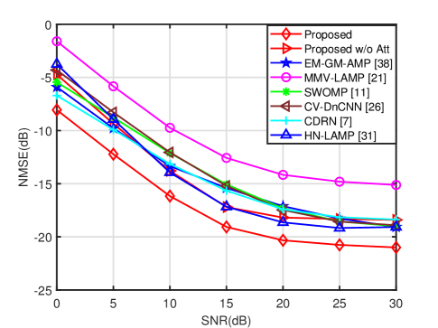
(a)

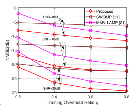
(b)

Figure 7: (a) Comparison of the NMSE versus SNR for hybrid IRS architecture at $T_{\mathsf{i}}=32$, $K=16$ and $G_{\mathsf{i}}=1024$. (b) Comparison of the NMSE versus training overhead at different SNR for the different estimation algorithms, where $\eta$ is defined as the ratio of the number of $T_{\mathsf{i}}$ to the $N_{\mathsf{i}}$.

V-D Comparison of the Iterations and Computational Complexity

The above experiments indicate that the hybrid driven methods perform well in CS. In the following, we further simulate the NMSE performance against the number of iterations to show the convergence of the proposed hybrid driven scheme. We compare two proposed schemes with MMV-LAMP and HN-LAMP, and the curve denoted by “Proposed w/o Res” means that the proposed schemes without residual learning mechanism.

Figure 8: NMSE versus iterations times under SNR = 15 dB. The curves on the left consider the passive IRS scenario with the same parameters in Fig. 5. The curves on the right consider the hybrid IRS scenario with the same parameters in Fig. 7.

Table III: Computational Complexity and Computation Time of Different Estimation Schemes

Schemes	Computational Complexity	Passive IRS	Hybrid IRS
		Execution Time (ms)	Execution Time (ms)
SWOMP [11]	$KGT\hat{L}$	/	/
EM-GM-GAMP [38]	$NKGT$	/	/
MMV-LAMP [21]	$NKGT$	31.18	13.92
CV-DnCNN [26]	$KGT\hat{L}+9N_{\mathsf{Dn}}N_{\mathsf{i}}N_{\mathsf{b}}k^{2}$	1131.68	34.84
CDRN [7]	$KGT\hat{L}+9N_{\mathsf{CD}}D_{\mathsf{CD}}N_{\mathsf{i}}N_{\mathsf{b}}k^{2}$	1131.27	34.88
HN-LAMP [31]	$NKGT+128NTK$	36.92	35.46
DA-RLAMP	$NKGT+$$9G\left(\left(L_{\mathsf{d}}+1\right)k^{2}+2\right)+6k^{2}$	37.16	/
MDA-RLAMP	$NKGT+$$G\left(L_{\mathsf{d}}\left(9k+k^{2}\right)+k^{2}+2\right)+6k^{2}$	/	17.94

Note: The learning methods are performed in Python 3.8 and Tensorflow 2.4 environment, while the conventional methods are executed in MATLAB. Therefore, the execution time of SWOMP and EM-GM-AMP is omitted.

Fig. 8 shows the curves of NMSE versus $N$ for different schemes. It can be observed that the estimation error of the proposed algorithms without residual learning is undulating as the number of iterations increases. In specific, the NMSE performance of DA-LAMP deteriorates when the number of iterations exceeds 6, and the MDA-LAMP method has a lower convergence rate during the training period. This is because the vanishing gradients problem hampers convergence as the number of iterations and parameters increase [29]. In constant, the proposed algorithms provide faster convergences at the early stage. Specifically, the DA-RLAMP (MDA-RLAMP) performs about 5 dB (2 dB) better than the network without residual learning and converges within 8 (10) layers. This phenomenon derives from the fact that the effectiveness of residual learning in complex networks, where each layer updates network parameters based on the result and information from the previous layers.

Besides, we outline the computational complexity of the proposed algorithms in online deployment. The computational cost of $L$ convolutional layers and $L$ depthwise convolution layers can be respectively expressed as [37]

$$\mathcal{O}\left(\sum_{j=1}^{L}\left(D_{\mathsf{h}}^{j}D_{\mathsf{w}}^{j}s_{\mathsf{k},j}^{2}n_{j-1}n_{j}\right)\right),$$ (46)

$$\mathcal{O}\left(\sum_{j=1}^{L}\left(D_{\mathsf{h}}^{j}D_{\mathsf{w}}^{j}s_{\mathsf{k},j}^{2}n_{j-1}\right)\right),$$ (47)

where the $j^{\mathsf{th}}$ convolution layer takes input tensor with size $D_{\mathsf{h}}^{j}\times D_{\mathsf{w}}^{j}\times n_{j-1}$ and uses kernel with size $s_{\mathsf{k},j}\times s_{\mathsf{k},j}\times n_{j-1}\times n_{j}$. The complexity of the DA-RLAMP in Algorithm 1 mainly stems include: i) The LAMP architecture, i.e., $\mathcal{O}(NKGT)$ for $K$ subcarriers; ii) $L_{\mathsf{d}}$ convolutional layers in DnCNN with computational complexity $\mathcal{O}\left(\sum_{j=1}^{L_{\mathsf{d}}}\left(Gs_{\mathsf{k},j}^{2}n_{j-1}n_{j}\right)\right)$; iii) $L_{\mathsf{s}}$ convolutional layers in spatial attention network with computational complexity $\mathcal{O}\left(\sum_{j=1}^{L_{\mathsf{s}}}\left(Gs_{\mathsf{k},j}^{2}n_{j-1}n_{j}\right)\right)$; iv) $L_{\mathsf{f}}$ layers in frequency attention network with computational complexity $\mathcal{O}\left(\sum_{j=1}^{L_{\mathsf{f}}}\left(m_{j-1}m_{j}\right)\right)$, where $m_{j}$ is the dimensions of the $j^{\mathsf{th}}$ layer output. As for the SWOMP algorithm, the complexity is $KGT$ for each iteration, and the algorithm will be repeated for a total of $\hat{L}$ iterations, where $\hat{L}$ denotes sufficient paths [24]. While the computational cost and execution time of the CV-DnCNN and CDRN come from the traditional channel estimation algorithms and deep learning networks. As described above, the computational complexity and time complexity of the proposed and other schemes are summarized in Table III. Thanks to the parallelization of a graphics processing unit, the execution time in online estimation can be greatly reduced. By contrast, the DA-RLAMP, MMV-LAMP and HN-LAMP have similar calculation times in the passive IRS scenario, while DA-RLAMP and MMV-LAMP consume less time than other schemes in the hybrid IRS scenario.

VI Conclusions

In this paper, we have proposed two hybrid driven networks to address the channel estimation problems for IRS aided frequency selective communication systems with hybrid architectures. Different from the existing deep learning aided network, we combine the data driven network and the model driven network to jointly enhance spatial and frequency properties and estimate channels. Meanwhile, we demonstrate how to leverage attention mechanisms and mobile networks for effective estimating hybrid IRS aided systems. Simulation results indicate that the proposed algorithms are capable of attaining significant performance improvements in terms of accuracy and pilot overhead.

References

• [1] Y. Liu, X. Liu, X. Mu, T. Hou, J. Xu, M. Di Renzo, and N. Al-Dhahir, “Reconfigurable Intelligent Surfaces: Principles and Opportunities,” IEEE Commun. Surveys Tuts., vol. 23, no. 3, pp. 1546–1577, Third Quarter 2021.
• [2] E. Basar, M. Di Renzo, J. De Rosny, M. Debbah, M.-S. Alouini, and R. Zhang, “Wireless Communications Through Reconfigurable Intelligent Surfaces,” IEEE Access, vol. 7, pp. 116 753–116 773, Aug. 2019.
• [3] Q. Wu and R. Zhang, “Intelligent Reflecting Surface Enhanced Wireless Network via Joint Active and Passive Beamforming,” IEEE Trans. Wireless Commun., vol. 18, no. 11, pp. 5394–5409, Nov. 2019.
• [4] J. Chen, Y.-C. Liang, Y. Pei, and H. Guo, “Intelligent reflecting surface: A programmable wireless environment for physical layer security,” IEEE Access, vol. 7, pp. 82 599–82 612, Jun. 2019.
• [5] X. Ma, Z. Chen, W. Chen, Z. Li, Y. Chi, C. Han, and S. Li, “Joint Channel Estimation and Data Rate Maximization for Intelligent Reflecting Surface Assisted Terahertz MIMO Communication Systems,” IEEE Access, vol. 8, pp. 99 565–99 581, May 2020.
• [6] P. Wang, J. Fang, H. Duan, and H. Li, “Compressed Channel Estimation for Intelligent Reflecting Surface-Assisted Millimeter Wave Systems,” IEEE Signal Process. Lett., vol. 27, pp. 905–909, May 2020.
• [7] C. Liu, X. Liu, D. W. K. Ng, and J. Yuan, “Deep Residual Learning for Channel Estimation in Intelligent Reflecting Surface-Assisted Multi-User Communications,” IEEE Trans. Wireless Commun., vol. 21, no. 2, pp. 898–912, Feb. 2022.
• [8] J. Chen, Y.-C. Liang, H. V. Cheng, and W. Yu, “Channel Estimation for Reconfigurable Intelligent Surface Aided Multi-User MIMO Systems,” arXiv preprint arXiv:1912.03619, Dec. 2019. [Online]. Available: https://arxiv.org/abs/1912.03619v1
• [9] C. Hu, L. Dai, S. Han, and X. Wang, “Two-Timescale Channel Estimation for Reconfigurable Intelligent Surface Aided Wireless Communications,” IEEE Trans. Commun., vol. 69, no. 11, pp. 7736–7747, Nov. 2021.
• [10] K. Venugopal, A. Alkhateeb, N. Gonzš¢lez Prelcic, and R. W. Heath, “Channel Estimation for Hybrid Architecture-Based Wideband Millimeter Wave Systems,” IEEE J. Sel. Areas Commun., vol. 35, no. 9, pp. 1996–2009, Sep. 2017.
• [11] J. Rodršªguez-Fernš¢ndez, N. Gonzš¢lez-Prelcic, K. Venugopal, and R. W. Heath, “Frequency-Domain Compressive Channel Estimation for Frequency-Selective Hybrid Millimeter Wave MIMO Systems,” IEEE Trans. Wireless Commun., vol. 17, no. 5, pp. 2946–2960, May 2018.
• [12] W. Zhang, J. Xu, W. Xu, D. W. K. Ng, and H. Sun, “Cascaded Channel Estimation for IRS-Assisted mmWave Multi-Antenna With Quantized Beamforming,” IEEE Commun. Lett., vol. 25, no. 2, pp. 593–597, Feb. 2021.
• [13] H. Ye, G. Y. Li, and B.-H. Juang, “Power of Deep Learning for Channel Estimation and Signal Detection in OFDM Systems,” IEEE Wireless Commun. Lett., vol. 7, no. 1, pp. 114–117, Feb. 2018.
• [14] A. Taha, M. Alrabeiah, and A. Alkhateeb, “Deep Learning for Large Intelligent Surfaces in Millimeter Wave and Massive MIMO Systems,” in 2019 IEEE Global Communications Conference (GLOBECOM), Dec. 2019, pp. 1–6.
• [15] E. Balevi and J. G. Andrews, “Wideband Channel Estimation With a Generative Adversarial Network,” IEEE Trans. Wireless Commun., vol. 20, no. 5, pp. 3049–3060, May 2021.
• [16] J. Gao, M. Hu, C. Zhong, G. Y. Li, and Z. Zhang, “An Attention-Aided Deep Learning Framework for Massive MIMO Channel Estimation,” IEEE Trans. Wireless Commun., vol. 21, no. 3, pp. 1823–1835, Mar. 2022.
• [17] M. Borgerding, P. Schniter, and S. Rangan, “AMP-Inspired Deep Networks for Sparse Linear Inverse Problems,” IEEE Trans. Signal Process., vol. 65, no. 16, pp. 4293–4308, Aug. 2017.
• [18] H. He, C.-K. Wen, S. Jin, and G. Y. Li, “Deep Learning-Based Channel Estimation for Beamspace mmWave Massive MIMO Systems,” IEEE Wireless Commun. Lett., vol. 7, no. 5, pp. 852–855, Oct. 2018.
• [19] S. Wu, L. Kuang, Z. Ni, D. Huang, Q. Guo, and J. Lu, “Message-Passing Receiver for Joint Channel Estimation and Decoding in 3D Massive MIMO-OFDM Systems,” IEEE Trans. Wireless Commun., vol. 15, no. 12, pp. 8122–8138, Dec. 2016.
• [20] X. Wei, C. Hu, and L. Dai, “Deep Learning for Beamspace Channel Estimation in Millimeter-Wave Massive MIMO Systems,” IEEE Trans. Commun., vol. 69, no. 1, pp. 182–193, Jan. 2021.
• [21] W. Zhu, M. Tao, X. Yuan, and Y. Guan, “Deep-Learned Approximate Message Passing for Asynchronous Massive Connectivity,” IEEE Trans. Wireless Commun., vol. 20, no. 8, pp. 5434–5448, Aug. 2021.
• [22] Y. Lin, S. Jin, M. Matthaiou, and X. You, “Tensor-Based Algebraic Channel Estimation for Hybrid IRS-Assisted MIMO-OFDM,” IEEE Trans. Wireless Commun., vol. 20, no. 6, pp. 3770–3784, Jun. 2021.
• [23] X. Lin, S. Wu, C. Jiang, L. Kuang, J. Yan, and L. Hanzo, “Estimation of Broadband Multiuser Millimeter Wave Massive MIMO-OFDM Channels by Exploiting Their Sparse Structure,” IEEE Trans. Wireless Commun., vol. 17, no. 6, pp. 3959–3973, Jun. 2018.
• [24] A. Abdallah, A. Celik, M. M. Mansour, and A. M. Eltawil, “Deep Learning-Based Frequency-Selective Channel Estimation for Hybrid mmWave MIMO Systems,” IEEE Trans. Wireless Commun., vol. 21, no. 6, pp. 3804–3821, Jun. 2022.
• [25] D. Tse and P. Viswanath, Fundamentals of Wireless Communication.   Cambridge university press, 2005.
• [26] S. Liu, Z. Gao, J. Zhang, M. D. Renzo, and M.-S. Alouini, “Deep Denoising Neural Network Assisted Compressive Channel Estimation for mmWave Intelligent Reflecting Surfaces,” IEEE Trans. Veh. Technol., vol. 69, no. 8, pp. 9223–9228, Aug. 2020.
• [27] S. Wu, H. Yao, C. Jiang, X. Chen, L. Kuang, and L. Hanzo, “Downlink Channel Estimation for Massive MIMO Systems Relying on Vector Approximate Message Passing,” IEEE Trans. Veh. Technol., vol. 68, no. 5, pp. 5145–5148, May 2019.
• [28] M. Ke, Z. Gao, Y. Wu, X. Gao, and R. Schober, “Compressive Sensing-Based Adaptive Active User Detection and Channel Estimation: Massive Access Meets Massive MIMO,” IEEE Trans. Signal Process., vol. 68, pp. 764–779, Jan. 2020.
• [29] K. He, X. Zhang, S. Ren, and J. Sun, “Deep Residual Learning for Image Recognition,” in 2016 IEEE Conference on Computer Vision and Pattern Recognition (CVPR), Jun. 2016, pp. 770–778.
• [30] X. Ma, Z. Gao, F. Gao, and M. Di Renzo, “Model-Driven Deep Learning Based Channel Estimation and Feedback for Millimeter-Wave Massive Hybrid MIMO Systems,” IEEE J. Sel. Areas Commun., vol. 39, no. 8, pp. 2388–2406, Aug. 2021.
• [31] W.-C. Tsai, C.-W. Chen, C.-F. Teng, and A.-Y. Wu, “Low-Complexity Compressive Channel Estimation for IRS-Aided mmWave Systems With Hypernetwork-Assisted LAMP Network,” IEEE Commun. Lett., vol. 26, no. 8, pp. 1883–1887, Aug. 2022.
• [32] A. L. Maas, A. Y. Hannun, A. Y. Ng et al., “Rectifier nonlinearities improve neural network acoustic models,” in Proc. icml, vol. 30, no. 1.   Atlanta, Georgia, USA, 2013, p. 3.
• [33] K. Zhang, W. Zuo, Y. Chen, D. Meng, and L. Zhang, “Beyond a Gaussian Denoiser: Residual Learning of Deep CNN for Image Denoising,” IEEE Trans. Image Process., vol. 26, no. 7, pp. 3142–3155, Jul. 2017.
• [34] S. Woo, J. Park, J.-Y. Lee, and I. S. Kweon, “Cbam: Convolutional block attention module,” in Proceedings of the European conference on computer vision (ECCV), Oct. 2018, pp. 3–19.
• [35] I. Goodfellow, Y. Bengio, and A. Courville, Deep Learning.   MIT press, 2016.
• [36] Z. Zhao, M. C. Vuran, F. Guo, and S. D. Scott, “Deep-Waveform: A Learned OFDM Receiver Based on Deep Complex-Valued Convolutional Networks,” IEEE J. Sel. Areas Commun., vol. 39, no. 8, pp. 2407–2420, Aug. 2021.
• [37] M. Sandler, A. Howard, M. Zhu, A. Zhmoginov, and L.-C. Chen, “MobileNetV2: Inverted Residuals and Linear Bottlenecks,” in 2018 IEEE/CVF Conference on Computer Vision and Pattern Recognition (CVPR), Jun. 2018, pp. 4510–4520.
• [38] J. P. Vila and P. Schniter, “Expectation-Maximization Gaussian-Mixture Approximate Message Passing,” IEEE Trans. Signal Process., vol. 61, no. 19, pp. 4658–4672, Oct. 2013.
• [39] D. P. Kingma and J. Ba, “Adam: A Method for Stochastic Optimization,” arXiv preprint arXiv:1412.6980, Dec. 2014.
• [40] T. Lin, J. Cong, Y. Zhu, J. Zhang, and K. Ben Letaief, “Hybrid Beamforming for Millimeter Wave Systems Using the MMSE Criterion,” IEEE Trans. Commun., vol. 67, no. 5, pp. 3693–3708, May 2019.