Blind Beamforming for Intelligent Reflecting Surface in Fading Channels without CSI

Abstract

This paper discusses how to optimize the phase shifts of intelligent reflecting surface (IRS) to combat channel fading without any channel state information (CSI), namely blind beamforming. Differing from most previous works based on a two-stage paradigm of first estimating channels and then optimizing phase shifts, our approach is completely data-driven, only requiring a dataset of the received signal power at the user terminal. Thus, our method does not incur extra overhead costs for channel estimation, and does not entail collaboration from service provider, either. The main idea is to choose phase shifts at random and use the corresponding conditional sample mean of the received signal power to extract the main features of the wireless environment. This blind beamforming approach guarantees an $N^{2}$ boost of signal-to-noise ratio (SNR), where $N$ is the number of reflective elements (REs) of IRS, regardless of whether the direct channel is line-of-sight (LoS) or not. Moreover, blind beamforming is extended to a double-IRS system with provable performance. Finally, prototype tests show that the proposed blind beamforming method can be readily incorporated into the existing communication systems in the real world; simulation tests further show that it works for a variety of fading channel models.

I Introduction

Intelligent reflecting surface (IRS), which is also referred to as reconfigurable intelligent surface (RIS), is envisioned to be a crucial wireless technology in future networks for its unique capability to improve the wireless environment by manipulating signal reflections. To fully exploit IRS, it entails judicious coordination of phase shifts across all the reflective elements (REs) of IRS, namely the IRS beamforming. Differing from many previous works that decide phase shifts based on channel estimation, this work advocates a blind beamforming strategy that does not require any channel knowledge. Furthermore, we analytically verify the performance of blind beamforming for the widely used Rician and Rayleigh fading models.

The proposed method builds upon a somewhat surprising fact that the reflected channels can be aligned with the direct channel (so as to maximize the overall channel) implicitly in the long run without knowing their real-time values and even without knowing their distribution parameters. All it needs is a set of first-moment statistics of the received signal, i.e., the conditional sample mean of the received signal power, which can be readily obtained in most wireless networks to date. Most importantly, the proposed blind beamforming policy does not require any collaboration between base-station and user terminal, so the overhead cost is literally zero. Thus, the IRS can be configured without any assistance from the service provider side.

The prior works about the IRS beamforming can be divided into two main categories according to the length of the channel coherence interval. One category of the existing works assumes that the channel coherence time interval is much longer than the blocklength, so the IRS beamforming is considered for a set of fixed direct and reflected channels, i.e., the static channel case. In contrast, the other category assumes short channel coherence so that the channels vary from time slot to time slot; as a result, the IRS beamforming is now considered for random channels and thus it aims at the average performance in the long run, i.e., the fading channel case.

As summarized in [1], many previous studies on the static channel case adopt the traditional paradigm of first estimating (static) channels and then optimizing phase shifts. After all the channels have been precisely acquired, the IRS beamforming amounts to a deterministic optimization problem for which the standard optimization methods work, e.g., [2, 3, 4, 5, 6, 7, 8] use semidefinite relaxation (SDR) [9], [10, 11, 12, 13, 14] use fractional programming [15, 16], and [17, 18] use minorization-maximization [19]. The above optimization methods are for continuous optimization, but the practical choice of phase shift is typically limited to a discrete set. To account for the discrete constraint, a natural idea [20, 21, 22] is to round the relaxed solution to the closest point in the discrete set. Clearly, the performance of the above model-driven IRS beamforming methods heavily depends on channel state information (CSI). Quite a few existing studies are devoted to channel acquisition for IRS, e.g., the ON-OFF method [23, 24] and the discrete Fourier transform (DFT) matrix method [25, 26, 27], but it can be hard to fit them into the current network protocol, not to mention the incurred complexity and latency. As a matter of fact, the existing prototype machines of IRS [28, 29, 30, 31] seldom use channel estimation.

Regarding the IRS beamforming in the fading channel case, the previous works mostly adopt the Rician/Rayleigh fading model and assume that the distribution parameters are perfectly known a priori. The goal is to seek a long-term solution of phase shifts to account for a large number of random channel realizations. Using Rician or Rayleigh fading model depends on whether the wireless propagation is blocked, i.e., the channel is modeled as Rician fading if it is line-of-sight (LoS), and is modeled as Rayleigh fading if it is the non-line-of-sight (NLoS). The authors of [32, 33, 34] assume that the reflected channels and the direct channel are all Rician fadings. Another popular setting [35, 36, 37, 38, 39, 40, 41, 42] is to assume that the reflected channels are Rician while the direct channel is Rayleigh; furthermore, [43, 44, 45] assume that the direct channel is completely blocked and thus equals zero. Assuming that the IRS has been placed in a bad position, [46, 47, 48, 49] assume that direct and reflected channels are all Rayleigh. Some more complicated fading models in the literature include the Kronecker correlation model [50], the double-scattering model [51], and the Nakagami-$m$ fading model [52, 53]. The present work assumes that the IRS has been well placed so that the reflected channels are all Rician, whereas the direct channel can be either Rician or Rayleigh.

A variety of optimization methods have been proposed for the IRS beamforming problem in the fading channel case, ranging from the projected gradient ascent method [54, 40, 50] to the complex circle manifold method [55, 45], the parallel coordinate descent method [36], the genetic algorithm [38, 41, 43], the particle swarm algorithm [56, 57], and the deep learning [34, 32, 58]. Moreover, [59] suggests a model-free gradient descent method by using a large dataset of historical channel values, the main idea of which is to predict the current channel distribution from past observations. Basically, the above methods all assume that the probability distribution of channel fading is either already known or predictable, but such statistical information for each single reflected channel can be costly to obtain when the IRS comprises massive REs. In contrast, our strategy only requires the first-moment statistics of the received signal power.

Because of the difficulties and cost of channel acquisition, there has been an increasing interest in configuring IRS without any channel information. For instance, [60] examines the expected achievable rate when the phase shifts are randomly selected; [61] proposes a distributed ascent algorithm for the continuous IRS beamforming based on the SNR feedback. Our work is most closely related to a line of studies that optimize the IRS beamforming based on the received signal power[28, 62, 63]. Specifically, [28] initiated the idea of deciding the ON-OFF status of each RE according to the corresponding conditional sample mean of received signal power, which was further developed in [62] to account for the discrete IRS beamforming. A more recent work shows that the above blind beamforming method can be readily extended to multiple IRSs. Nevertheless, this paper can be distinguished from these existing works in that it considers blind beamforming for the fading channel case whereas [60, 61, 28, 62, 63] all assume the static channel case.

The rest of the paper is organized as follows. Section II describes the system model and problem formulation. Section III proposes a blind beamforming method when the direct channel is LoS. Section IV discusses some subtle issues with the NLoS case and proposes an improved blind beamforming method. Section V extends the proposed algorithms to a double-IRS system. Section VI shows the numerical results. Finally, Section VII concludes the paper.

We use the Bachmann-Landau notation extensively in the paper: $f(n)=O(g(n))$ if there exists some $c>0$ such that $|f(n)|\leq cg(n)$ for $n$ sufficiently large; $f(n)=o(g(n))$ if there exists some $c>0$ such that $|f(n)|<cg(n)$ for $n$ sufficiently large; $f(n)=\Omega(g(n))$ if there exists some $c>0$ such that $f(n)\geq cg(n)$ for $n$ sufficiently large; $f(n)=\Theta(g(n))$ if $f(n)=O(g(n))$ and $f(n)=\Omega(g(n))$.

II System Model

Consider an IRS-assisted point-to-point wireless transmission. Assume that the transmitter and receiver have one antenna each, and that the IRS comprises $N$ REs. Every RE induces a reflected channel from the transmitter to the receiver. Let $h_{n}\in\mathbb{C}$ be the reflected channel due to RE $n=1,\ldots,N$ and let $h_{0}\in\mathbb{C}$ be the superposition of the remaining channels aside from the reflected channels—which is referred to as the direct channel. In particular, each reflected channel $h_{n}$ can be factored as

$$h_{n}=f_{n}g_{n},$$ (1)

where $f_{n}\in\mathbb{C}$ is the channel from the transmitter to RE $n$ and $g_{n}\in\mathbb{C}$ is the channel from RE $n$ to the receiver. Furthermore, the above channels are modeled as

$$h_{0}=\sqrt{\gamma_{00}}\left(\sqrt{\frac{\delta_{00}}{1+\delta_{00}}}\overline{h}_{0}+\sqrt{\frac{1}{1+\delta_{00}}}\widetilde{h}_{0}\right),$$ (2a)

$$f_{n}=\sqrt{\gamma_{0n}}\left(\sqrt{\frac{\delta_{0n}}{1+\delta_{0n}}}\overline{f}_{n}+\sqrt{\frac{1}{1+\delta_{0n}}}\widetilde{f}_{n}\right),$$ (2b)

$$g_{n}=\sqrt{\gamma_{n0}}\left(\sqrt{\frac{\delta_{n0}}{1+\delta_{n0}}}\overline{g}_{n}+\sqrt{\frac{1}{1+\delta_{n0}}}\widetilde{g}_{n}\right),$$ (2c)

where $\gamma_{00},\gamma_{0n},\gamma_{n0}\in[0,1]$ are the channel attenuation, $\overline{h}_{0},\overline{f}_{n},\overline{g}_{n}$ are normalized complex constants so that $|\overline{h}_{0}|=|\overline{f}_{n}|=|\overline{g}_{n}|=1$, $\widetilde{h}_{0},\widetilde{f}_{n},\widetilde{g}_{n}\sim\mathcal{CN}(0,1)$ are the standard complex Gaussian random variables, and $\delta_{00},\delta_{0n},\delta_{n0}\geq 0$ are the Rician factors [64]. In principle, the Rician factor decreases as the channel becomes more blocked. We remark that the above variables are all unknown in the assumed system model.

Moreover, substituting (2b) and (2c) into (1) decomposes each reflected channel $h_{n}$ as

$$h_{n}=\sqrt{\gamma_{0n}\gamma_{n0}}\,\times$$

$$\left(\sqrt{\frac{\delta_{0n}\delta_{n0}}{(1+\delta_{0n})(1+\delta_{n0})}}\overline{h}_{n}+\sqrt{\frac{1}{(1+\delta_{0n})(1+\delta_{n0})}}\widetilde{h}_{n}\right),$$ (3)

where

$$\overline{h}_{n}=\overline{f}_{n}\overline{g}_{n},$$ (4a)

$$\widetilde{h}_{n}=\sqrt{\delta_{0n}}\overline{f}_{n}\widetilde{g}_{n}+\sqrt{\delta_{n0}}\widetilde{f}_{n}\overline{g}_{n}+\widetilde{f}_{n}\widetilde{g}_{n}.$$ (4b)

Let $\theta_{n}\in[0,2\pi)$ be the phase shift of RE $n$. With the additive noise $Z\in\mathbb{C}$ and the transmit signal $X\in\mathbb{C}$, the received signal $Y\in\mathbb{C}$ is given by

$$Y=\left(h_{0}+\sum_{n=1}^{N}h_{n}e^{j\theta_{n}}\right)X+Z.$$ (5)

Assuming that $Z\sim\mathcal{CN}(0,\sigma^{2})$ is complex Gaussian with a power of $\sigma^{2}$ and that $X$ meets the mean power constraint $P$, i.e., $\mathbb{E}[|X|^{2}]\leq P$, an achievable ergodic data rate is given by

$$R=\mathbb{E}\left[\mathrm{log}\left(1+\frac{P}{\sigma^{2}}\bigg{|}h_{0}+\sum_{n=1}^{N}h_{n}e^{j\theta_{n}}\bigg{|}^{2}\right)\right]$$ (6)

with the expectation taken over all the random fading components $\{\widetilde{h}_{0},\widetilde{f}_{n},\widetilde{g}_{n}\}$. The above rate expression can be difficult to tackle directly. A common idea in the existing literature [35, 36, 33, 34, 39] is to move the expectation to the inside of log; the resulting approximation is an upper bound on $R$:

$$R\leq\mathrm{log}\left(1+\frac{P}{\sigma^{2}}\cdot\mathbb{E}\left[\bigg{|}h_{0}+\sum_{n=1}^{N}h_{n}e^{j\theta_{n}}\bigg{|}^{2}\right]\right).$$ (7)

Notice that maximizing the above upper bound amounts to maximizing the expectation of the overall channel power.

Each phase shift $\theta_{n}$ in practice must take on values from the discrete set

$$\Phi_{K}=\{\omega,2\omega,\ldots,K\omega\}\;\,\text{where}\;\,\omega=\frac{2\pi}{K}$$ (8)

given an integer $K\geq 2$. We seek the optimal phase shift array $\bm{\theta}=(\theta_{1},\ldots,\theta_{N})$ to maximize the expectation of the overall channel power in the long run:

$$\underset{\bm{\theta}}{\text{maximize}}\quad\mathbb{E}\left[\bigg{|}h_{0}+\sum_{n=1}^{N}h_{n}e^{j\theta_{n}}\bigg{|}^{2}\right]$$ (9a)

$$\text{subject to}\quad\theta_{n}\in\Phi_{K},\;\text{for}\;n=1,\ldots,N.$$ (9b)

The difficulties of the above problem can be recognized in two respects. First, the variables $\{\theta_{n}\}$ to optimize are discrete. Second, more importantly, none of the channel parameters $\{\gamma_{00},\gamma_{0n},\gamma_{n0},\overline{h}_{0},\overline{f}_{n},\overline{g}_{n},\delta_{00},\delta_{0n},\delta_{n0}\}$ is available.

Our goal is to solve (9) without any channel information, namely blind beamforming. The proposed method depends on whether the direct channel $h_{0}$ is LoS or not (i.e., whether the $|\mathbb{E}[h_{0}]|$ is large or not) as illustrated in Fig. 1. The following two sections deal with the LoS and the NLoS cases separately.

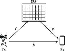
(a) LoS direct channel case

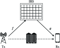
(b) NLoS direct channel case

Figure 1: Two possible channel models of the IRS-assisted transmission.

III LoS Direct Channel Case

In this section, we focus on the LoS direct channel case with sufficiently large $\delta_{00}$ so that the fixed fading component $\overline{h}_{0}$ is not negligible as compared to the random fading component $\widetilde{h}_{0}$. We first optimize $\bm{\theta}$ assuming that CSI is known, and then discuss how to eliminate the need for CSI by statistics.

III-A Model-Driven IRS Beamforming with CSI

We start by ignoring the discrete constraint (9b) so that the phase shift variables $\theta_{n}$ can be continuously chosen; alternatively, this can be thought of as the extremal case with $K\rightarrow\infty$. The resulting continuous approximation can provide an upper bound on the global optimum of the discrete case.

Let $\Delta_{n}$ denote the phase difference between each reflected channel $h_{n}$ and the direct channel $h_{0}$ in terms of their fixed fading components:

$$\Delta_{n}=\angle\overline{h}_{0}-\angle\overline{h}_{n},\;\text{for}\;n=1,\ldots,N.$$ (10)

The following proposition shows that setting each $\theta_{n}$ to $\Delta_{n}$ is optimal for the continuous IRS beamforming.

Proposition 1

Assuming that CSI is known and the number of phase shift choices $K\rightarrow\infty$, the maximum expected overall channel power in (9a) is achieved by letting $\theta_{n}^{\star}=\Delta_{n}$.

Proof:

The expected overall channel power can be expanded and then bounded as

$$\mathbb{E}\left[\bigg{|}h_{0}+\sum_{n=1}^{N}h_{n}e^{j\theta_{n}}\bigg{|}^{2}\right]$$

$$=\mathbb{E}\Bigg{[}\Bigg{|}\sqrt{\frac{\gamma_{00}\delta_{00}}{1+\delta_{00}}}\overline{h}_{0}+\sum_{n=1}^{N}\sqrt{\frac{\gamma_{0n}\gamma_{n0}\delta_{0n}\delta_{n0}}{(1+\delta_{0n})(1+\delta_{n0})}}\overline{h}_{n}e^{j\theta_{n}}$$

$$\quad+\sqrt{\frac{\gamma_{00}}{1+\delta_{00}}}\widetilde{h}_{0}+\sum_{n=1}^{N}\sqrt{\frac{\gamma_{0n}\gamma_{n0}}{(1+\delta_{0n})(1+\delta_{n0})}}\widetilde{h}_{n}e^{j\theta_{n}}\Bigg{|}^{2}\Bigg{]}$$

$$\stackrel{{\scriptstyle(a)}}{{=}}\left|\sqrt{\frac{\gamma_{00}\delta_{00}}{1+\delta_{00}}}\overline{h}_{0}+\sum_{n=1}^{N}\sqrt{\frac{\gamma_{0n}\gamma_{n0}\delta_{0n}\delta_{n0}}{(1+\delta_{0n})(1+\delta_{n0})}}\overline{h}_{n}e^{j\theta_{n}}\right|^{2}$$

$$\quad+\frac{\gamma_{00}}{1+\delta_{00}}+\sum_{n=1}^{N}\frac{\gamma_{0n}\gamma_{n0}(\delta_{0n}+\delta_{n0}+1)}{(1+\delta_{0n})(1+\delta_{n0})}$$

$$\stackrel{{\scriptstyle(b)}}{{\leq}}\left(\sqrt{\frac{\gamma_{00}\delta_{00}}{1+\delta_{00}}}\big{|}\overline{h}_{0}\big{|}+\sum_{n=1}^{N}\sqrt{\frac{\gamma_{0n}\gamma_{n0}\delta_{0n}\delta_{n0}}{(1+\delta_{0n})(1+\delta_{n0})}}\big{|}\overline{h}_{n}\big{|}\right)^{2}$$

$$\quad+\frac{\gamma_{00}}{1+\delta_{00}}+\sum_{n=1}^{N}\frac{\gamma_{0n}\gamma_{n0}(\delta_{0n}+\delta_{n0}+1)}{(1+\delta_{0n})(1+\delta_{n0})}$$

$$\stackrel{{\scriptstyle(c)}}{{=}}\left(\sqrt{\frac{\gamma_{00}\delta_{00}}{1+\delta_{00}}}+\sum_{n=1}^{N}\sqrt{\frac{\gamma_{0n}\gamma_{n0}\delta_{0n}\delta_{n0}}{(1+\delta_{0n})(1+\delta_{n0})}}\right)^{2}$$

$$\quad+\frac{\gamma_{00}}{1+\delta_{00}}+\sum_{n=1}^{N}\frac{\gamma_{0n}\gamma_{n0}(\delta_{0n}+\delta_{n0}+1)}{(1+\delta_{0n})(1+\delta_{n0})},$$ (11)

where $(a)$ follows since $\widetilde{h}_{0},\widetilde{h}_{n},\ldots,\widetilde{h}_{N}$ are all zero-mean and $\mathbb{E}[|\widetilde{h}_{n}|^{2}]=\delta_{0n}+\delta_{n0}+1$, $(b)$ follows by the triangle inequality wherein the equality holds if every

$$\theta_{n}=\Delta_{n},$$ (12)

and $(c)$ follows since $\{\overline{h}_{0},\overline{h}_{n}\}$ are all normalized complex numbers. The proof is then completed. ∎

But what if $K$ is a finite integer? A natural idea is to round the continuous solution to the closest point in the discrete set $\Phi_{K}$, namely closest point projection (CPP):

$$\theta_{n}^{\mathrm{CPP}}=\arg\min_{\theta_{n}\in\Phi_{K}}\left\{\left|\theta_{n}-\Delta_{n}\right|\;\text{mod}\,{2\pi}\right\}.$$ (13)

As the main result of this subsection, the following proposition shows that the CPP method guarantees a constant approximation factor when $K$ is fixed.

Proposition 2

Assuming that CSI is known and $K<\infty$, the expected overall channel power with $\theta_{n}^{\mathrm{CPP}}$ in (13) satisfies

$$\cos^{2}(\frac{\pi}{K})\cdot f^{\star}\leq\mathbb{E}\left[\bigg{|}h_{0}+\sum_{n=1}^{N}h_{n}e^{j\theta_{n}^{\mathrm{CPP}}}\bigg{|}^{2}\right]\leq f^{\star},$$ (14)

where $f^{\star}$ refers to the maximum possible expected channel power under the discrete constraint.

Proof:

The upper bound is evident. We just concentrate on the lower bound in what follows. It can be shown that

$$\mathbb{E}\left[\bigg{|}h_{0}+\sum_{n=1}^{N}h_{n}e^{j\theta_{n}^{\mathrm{CPP}}}\bigg{|}^{2}\right]$$

$$=\left|\sqrt{\frac{\gamma_{00}\delta_{00}}{1+\delta_{00}}}+\sum_{n=1}^{N}\sqrt{\frac{\gamma_{0n}\gamma_{n0}\delta_{0n}\delta_{n0}}{(1+\delta_{0n})(1+\delta_{n0})}}e^{j(\theta_{n}^{\mathrm{CPP}}-\Delta_{n})}\right|^{2}$$

$$\quad+\frac{\gamma_{00}}{1+\delta_{00}}+\sum_{n=1}^{N}\frac{\gamma_{0n}\gamma_{n0}(\delta_{0n}+\delta_{n0}+1)}{(1+\delta_{0n})(1+\delta_{n0})}$$

$${\geq}\left(\sqrt{\frac{\gamma_{00}\delta_{00}}{1+\delta_{00}}}+\cos(\frac{\pi}{K})\cdot\sum_{n=1}^{N}\sqrt{\frac{\gamma_{0n}\gamma_{n0}\delta_{0n}\delta_{n0}}{(1+\delta_{0n})(1+\delta_{n0})}}\right)^{2}$$

$$\quad+\frac{\gamma_{00}}{1+\delta_{00}}+\sum_{n=1}^{N}\frac{\gamma_{0n}\gamma_{n0}(\delta_{0n}+\delta_{n0}+1)}{(1+\delta_{0n})(1+\delta_{n0})}$$

$$\geq\cos^{2}(\frac{\pi}{K})\cdot\left(\sqrt{\frac{\gamma_{00}\delta_{00}}{1+\delta_{00}}}+\sum_{n=1}^{N}\sqrt{\frac{\gamma_{0n}\gamma_{n0}\delta_{0n}\delta_{n0}}{(1+\delta_{0n})(1+\delta_{n0})}}\right)^{2}$$

$$\quad+\cos^{2}(\frac{\pi}{K})\cdot\left(\frac{\gamma_{00}}{1+\delta_{00}}+\sum_{n=1}^{N}\frac{\gamma_{0n}\gamma_{n0}(\delta_{0n}+\delta_{n0}+1)}{(1+\delta_{0n})(1+\delta_{n0})}\right).$$ (15)

Comparing (15) with the upper bound on $f^{\star}$ in (11) establishes the lower bound in (14). ∎

With the above result, the asymptotic performance of the CPP method as $N\rightarrow\infty$ immediately follows, as stated in the following corollary.

Corollary 1

When $K>2$, the expected channel power with $\theta_{n}^{\mathrm{CPP}}$ in (13) satisfies

$$\mathbb{E}\left[\left|h_{0}+\sum_{n=1}^{N}h_{n}e^{j\theta_{n}^{\mathrm{CPP}}}\right|^{2}\right]=\Theta(N^{2}),$$ (16)

where the expectation is taken over random fading channels.

Remark 1

For the binary beamforming case with $K=2$, i.e., when each $\theta_{n}\in\{0,\pi\}$, the quadratic boost in (16) by CPP is no longer guaranteed, as shown in the following example. Assume that all the reflected channel magnitudes $|h_{n}|$ are equal; assume also that $\Delta_{n}=\pi/2-\varepsilon$ for $n=1,\ldots,N/2$ and $\Delta_{n}=-\pi/2+\varepsilon$ for $n=N/2+1,\ldots,N$. Let $\varepsilon\rightarrow 0^{+}$. Consequently, according to (13), we have $\theta_{n}^{\mathrm{CPP}}=0$ for every $n=1,\ldots,N$ and hence the left-hand side in (16) approaches 1. Actually, it is optimal to let $\theta_{n}^{\mathrm{CPP}}=0$ for $n=1,\ldots,N/2$ and let $\theta_{n}^{\mathrm{CPP}}=\pi$ for $n=1,\ldots,N/2$, and then the quadratic boost in (16) holds.

Remark 2

Actually, the global optimum of (9) can be achieved by a linear-time algorithm in [65] provided that CSI is available. However, it is difficult to perform this algorithm blindly without channel acquisition. In the rest of this paper, we shall assume that $K>2$ so that the CPP method is good enough.

III-B Data-Driven IRS beamforming without CSI

It turns out that the CPP method can be implemented even in the absence of CSI. The key idea is to choose $(\theta_{1},\ldots,\theta_{N})$ at random and then utilize the resulting expectation, which has been considered in [28, 62]. It is worth emphasizing the distinction between [28, 62] and the present work. The former assumes static channels so that the expectation is over the random phase shifts $\theta_{n}$, while the latter assumes fading channels so that the expectation is over both $\theta_{n}$ and the random fading channels.

We start our discussion by computing the conditional expectation of the received signal power when a particular phase shift $\theta_{n}$ is fixed to be $\varphi\in\Phi_{K}$:

$$\mathbb{E}\left[|Y|^{2}\big{|}\theta_{n}=\varphi\right]$$

$$=2P\sqrt{\frac{\gamma_{00}\gamma_{0n}\gamma_{n0}\delta_{00}\delta_{0n}\delta_{n0}}{(1+\delta_{00})(1+\delta_{0n})(1+\delta_{n0})}}\cos(\varphi-\Delta_{n})+\sigma^{2}\,+$$

$$\qquad\quad P\left(\gamma_{00}+\sum_{n=1}^{N}\frac{\gamma_{0n}\gamma_{n0}(\delta_{0n}\delta_{n0}+\delta_{0n}+\delta_{n0}+1)}{(1+\delta_{0n})(1+\delta_{n0})}\right).$$ (17)

Clearly, when treated as a function of $\varphi$, the above conditional expectation is maximized when the gap between $\varphi$ and $\Delta_{n}$ modulo $2\pi$ is minimized; interestingly, this optimal $\varphi$ can be recognized as the CPP solution in (13).

Thus, we can recover the CPP solution in (13) even without knowing CSI. All we need is just a set of conditional expectations $\{\mathbb{E}\left[|Y|^{2}\big{|}\theta_{n}=\varphi\right]:n=1,\ldots,N,\varphi\in\Phi_{K}\}$, which can be empirically obtained from the signal power measure. Specifically, we first generate a total of $T$ random samples of $\bm{\theta}$ in an i.i.d. fashion. Denote by $\mathcal{Q}_{nk}\subseteq\{1,\ldots,T\}$ the subset of random samples with $\theta_{nt}=k\omega$, for $n=1,\ldots,N$ and $k=1,\ldots,K$. The sample mean of the received signal power $\left|Y_{t}\right|^{2}$ conditioned on each $\mathcal{Q}_{nk}$ is given by

$$\widehat{\mathbb{E}}\left[|Y|^{2}\mid\theta_{n}=k\omega\right]=\frac{1}{\left|\mathcal{Q}_{nk}\right|}\sum_{t\in\mathcal{Q}_{nk}}|Y_{t}|^{2}.$$ (18)

The CSM method chooses each $\theta_{n}$ to maximize the corresponding conditional sample mean, i.e.,

$$\theta_{n}^{\mathrm{CSM}}=\arg\max_{\varphi\in\Phi_{K}}\widehat{\mathbb{E}}\left[|Y|^{2}\mid\theta_{n}=\varphi\right].$$ (19)

The above procedure is summarized in Algorithm 1. We further analyze its performance in the following proposition.

Algorithm 1 Conditional Sample Mean (CSM)

1:input: $\Phi_{K}$ and $N$.

2:for $t=1,2,\ldots,T$ do

3:     Generate $\bm{\theta}_{t}=(\theta_{1t},\ldots\theta_{Nt})$ i.i.d. based on $\Phi_{K}$.

4:     Measure received signal power $\left|Y_{t}\right|^{2}$ with $\bm{\theta}_{t}$.

5:end for

6:for $n=1,2,\ldots,N$ do

7:     for $k=1,2,\ldots,K$ do

8:         Compute $\widehat{\mathbb{E}}\left[|Y|^{2}\mid\theta_{n}=k\omega\right]$ according to (18).

9:     end for

10:     Decide $\theta_{n}^{\mathrm{CSM}}$ according to (19).

11:end for

12:output: $\bm{\theta}^{\mathrm{CSM}}=\left(\theta_{1}^{\mathrm{CSM}},\ldots,\theta_{N}^{\mathrm{CSM}}\right)$.

Proposition 3

If $K>2$ and $\mathbb{E}[h_{0}]$ is bounded away from zero, then the expectation of the overall channel power in the long run achieved by CSM satisfies

$$\mathbb{E}\left[\left|h_{0}+\sum_{n=1}^{N}h_{n}e^{j\theta_{n}^{\mathrm{CSM}}}\right|^{2}\right]=\Theta(N^{2})$$ (20)

as $T\rightarrow\infty$, where the expectation is taken over both random samples of $\bm{\theta}$ as well as random fading channels.

Proof:

Conditioned on $\theta_{n}=\varphi$, since the rest phase shift variables are selected randomly and independently, the sample value $|Y|^{2}$ can be recognized as an i.i.d. random variable; moreover, it is evident that the variance of $|Y|^{2}$ is bounded. Then, by the law of large numbers, we have the sample mean $\widehat{\mathbb{E}}\left[|Y|^{2}\mid\theta_{n}=k\omega\right]$ converge to the actual mean $\mathbb{E}\left[|Y|^{2}\mid\theta_{n}=k\omega\right]$ as $T\rightarrow\infty$. Combining the above result with (14) verifies (20). ∎

IV NLoS Direct Channel Case

A subtle condition in Proposition 3 requires the expected direct channel, $\mathbb{E}[h_{0}]$, to be bounded away from zero. But why is this condition necessary for the proposed blind beamforming algorithm to work? And how do we make our algorithm continue to work if the condition is violated? The following two subsections provide answers to the above two questions, respectively.

IV-A CSM may Fail if $\mathbb{E}[h_{0}]$ is Small

We begin with the extreme case with $\mathbb{E}[h_{0}]=0$, i.e., when the direct propagation is completely blocked. Notice that $E[h_{0}]=0$ implies either $\gamma_{00}=0$ or $\delta_{00}=0$. Consequently, the conditional expectation in (III-B) reduces to

$$\mathbb{E}\left[|Y|^{2}\big{|}\theta_{n}=\varphi\right]=P\sum_{n=1}^{N}\frac{\gamma_{0n}\gamma_{n0}(\delta_{0n}\delta_{n0}+\delta_{0n}+\delta_{n0}+1)}{(1+\delta_{0n})(1+\delta_{n0})}\\ +\sigma^{2}+P\gamma_{00},$$ (21)

which does not depend on the choice of $\theta_{n}$. Thus, even if the $\widehat{\mathbb{E}}\left[|Y|^{2}\mid\theta_{n}=k\omega\right]$ converges to $\mathbb{E}\left[|Y|^{2}\mid\theta_{n}=k\omega\right]$, we cannot decide each $\theta_{n}$ as in (19).

But if $\mathbb{E}[h_{0}]$ is only arbitrarily close to zero, is it possible to compensate by letting $T\rightarrow\infty$? To see the answer, we now expand the conditional sample mean in (18) as

$$\widehat{\mathbb{E}}\left[|Y|^{2}\mid\theta_{n}=\varphi\right]=2P\beta_{1}\cos(\varphi-\Delta_{n})+\sum^{7}_{i=1}C_{i},$$ (22)

where

$$C_{1}=\frac{2P}{\left|\mathcal{Q}_{nk}\right|}\sum_{t\in\mathcal{Q}_{nk}}\sum_{n=0}^{N}|h_{nt}|^{2},$$

$$C_{2}=\frac{2P}{\left|\mathcal{Q}_{nk}\right|}\sum_{t\in\mathcal{Q}_{nk}}\mathfrak{Re}\left\{\beta_{2}\overline{h}^{H}_{0}\widetilde{h}_{nt}+\beta_{3}\widetilde{h}^{H}_{0t}\overline{h}_{n}+\beta_{4}\widetilde{h}^{H}_{0t}\widetilde{h}_{nt}\right\},$$

$$C_{3}=\frac{2P}{\left|\mathcal{Q}_{nk}\right|}\sum_{t\in\mathcal{Q}_{nk}}\mathfrak{Re}\Bigg{\{}h^{H}_{0t}\sum_{m=1,m\neq n}^{N}h_{mt}e^{j\theta_{mt}}\Bigg{\}},$$

$$C_{4}=\frac{2P}{\left|\mathcal{Q}_{nk}\right|}\sum_{t\in\mathcal{Q}_{nk}}\mathfrak{Re}\Bigg{\{}h^{H}_{nt}\sum_{m=1,m\neq n}^{N}h_{mt}e^{j(\theta_{mt}-\varphi)}\Bigg{\}},$$

$$C_{5}=\frac{2P}{\left|\mathcal{Q}_{nk}\right|}\sum_{t\in\mathcal{Q}_{nk}}\mathfrak{Re}\Bigg{\{}\sum_{a=1}^{N}\sum_{b=1,b\neq a}^{N}h_{at}h^{H}_{bt}e^{j\left(\theta_{at}-\theta_{bt}\right)}\Bigg{\}},$$

$$C_{6}=\frac{2\sqrt{P}}{\left|\mathcal{Q}_{nk}\right|}\sum_{t\in\mathcal{Q}_{nk}}\mathfrak{Re}\Bigg{\{}\sum_{n=0}^{N}h_{nt}e^{j\theta_{nt}}Z^{H}_{t}\Bigg{\}},$$

$$C_{7}=\frac{1}{\left|\mathcal{Q}_{nk}\right|}\sum_{t\in\mathcal{Q}_{nk}}\left|Z_{t}\right|^{2},$$

$$\beta_{1}=\sqrt{\frac{\gamma_{00}\gamma_{0n}\gamma_{n0}\delta_{00}\delta_{0n}\delta_{n0}}{(1+\delta_{00})(1+\delta_{0n})(1+\delta_{n0})}},$$

$$\beta_{2}=\sqrt{\frac{\gamma_{00}\gamma_{0n}\gamma_{n0}\delta_{00}}{(1+\delta_{00})(1+\delta_{0n})(1+\delta_{n0})}},$$

$$\beta_{3}=\sqrt{\frac{\gamma_{00}\gamma_{0n}\gamma_{n0}\delta_{0n}\delta_{n0}}{(1+\delta_{00})(1+\delta_{0n})(1+\delta_{n0})}},$$

$$\beta_{4}=\sqrt{\frac{\gamma_{00}\gamma_{0n}\gamma_{n0}}{(1+\delta_{00})(1+\delta_{0n})(1+\delta_{n0})}}.$$

Recall that the aim of CSM is to get $\bm{\theta}^{\mathrm{CSM}}=\bm{\theta}^{\mathrm{CPP}}$. Toward this end, it requires that $\widehat{\mathbb{E}}\left[|Y|^{2}\mid\theta_{n}=\theta^{\mathrm{CPP}}\right]>\widehat{\mathbb{E}}\left[|Y|^{2}\mid\theta_{n}=\varphi\right]$ holds for any $\varphi\neq\theta^{\mathrm{CPP}}$ since we choose each $\theta_{n}$ to maximize the conditional sample mean as in (19); it is sufficient to require that

$$\left|\widehat{\mathbb{E}}\left[|Y|^{2}\mid\theta_{n}=\varphi\right]-{\mathbb{E}}\left[|Y|^{2}\mid\theta_{n}=\varphi\right]\right|<2\beta_{1}\epsilon_{n}$$ (23)

where $\epsilon_{n}>0$ is the difference between the highest value and the second highest value of $\cos\left(\varphi-\Delta_{n}\right)$ across all possible $\varphi\in\Phi_{K}$. Intuitively speaking, if each conditional sample mean is close to its real expectation, then we will not get confused with the actual $\theta_{n}$ that maximizes ${\mathbb{E}}\left[|Y|^{2}\mid\theta_{n}=\varphi\right]$.

Based on the above observation, we can bound the probability of error as

$$\operatorname{Pr}\left\{\bm{\theta}^{\mathrm{CSM}}\neq\bm{\theta}^{\mathrm{CPP}}\right\}$$

$$\stackrel{{\scriptstyle(a)}}{{\leq}}\sum_{n=1}^{N}\operatorname{Pr}\left\{\theta_{n}^{\mathrm{CSM}}\neq\theta_{n}^{\mathrm{CPP}}\right\}$$

$$\leq\sum_{n=1}^{N}\operatorname{Pr}\left\{\left|\widehat{\mathbb{E}}\left[|Y|^{2}\mid\theta_{n}=\varphi\right]-{\mathbb{E}}\left[|Y|^{2}\mid\theta_{n}=\varphi\right]\right|>2\beta_{1}\epsilon_{n}\right\}$$

$$\stackrel{{\scriptstyle(b)}}{{\leq}}\sum_{n=1}^{N}\frac{\operatorname{Var}(\sum^{7}_{i=1}C_{i})}{4\left|\mathcal{Q}_{nk}\right|\beta_{1}^{2}\epsilon_{n}^{2}}$$

$$\stackrel{{\scriptstyle(c)}}{{\simeq}}\sum_{n=1}^{N}\frac{K(1+\delta_{00})(1+\delta_{0n})(1+\delta_{n0})\cdot\operatorname{Var}(\sum^{7}_{i=1}C_{i})}{4T\gamma_{00}\gamma_{0n}\gamma_{n0}\delta_{00}\delta_{0n}\delta_{n0}\epsilon_{n}^{2}},$$ (24)

where $(a)$ follows by the union bound, $(b)$ follows by Chebyshev’s inequality, and $(c)$ follows since $\left|\mathcal{Q}_{nk}\right|\approx T/K$.

The above upper bound suggests that just letting $T\rightarrow\infty$ may not be enough for the CSM algorithm to achieve the quadratic boost as stated in Proposition 3 in the NLoS direct channel case. Rather, it requires

$$T=\Omega\left(\frac{1}{\gamma_{00}\delta_{00}}\right).$$ (25)

In the remainder of this section, we propose an improved version of CSM called Grouped Conditional Sample Mean (GCSM), which (i) still works when $\mathbb{E}[h_{0}]=0$ and (ii) does not incur many more samples as in (25) when $\mathbb{E}[h_{0}]\rightarrow 0$.

Remark 3

The above result implies that we can tell the status (LoS or NLoS) of the direct channel without CSI. We just compare the values of $\widehat{\mathbb{E}}\left[|Y|^{2}\mid\theta_{n}=\varphi\right]$ with different $\varphi$; the direct channel is NLoS if these conditional sample means are close, and is LoS otherwise.

IV-B Grouped Conditional Sample Mean (GCSM)

Since $|\mathbb{E}[h_{0}]|$ being too small is the cause of the above issues, a natural idea is to make $|\mathbb{E}[h_{0}]|$ larger by incorporating some reflected channels into $h_{0}$. Following this idea, a naive algorithm is to divide the reflected channels into two groups and perform CSM between them alternatively. Specifically, for each iteration, we optimize $\theta_{n}$’s in one group by CSM while fixing the other group. But the performance of this alternating CSM cannot be justified, as illustrated by a toy example shown in Fig. 2; the main reason is that in each step CSM can only guarantee an approximation ratio but cannot guarantee that the optimized result is better than the previous one.

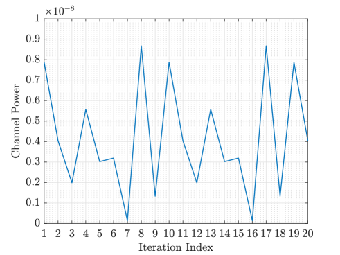
Figure 2: An example of CSM with the set of reflected channels is divided into two groups. Assume that $N=4$ and the channels are $[h_{0},h_{1},h_{2},h_{3},h_{4}]=[0,1.7646+2.1012j,0.2792-1.6644j,0.7178+3.1842j,0.6117-2.2282j]\times 10^{-5}$; the reflected channels are grouped as $S_{\mathrm{I}}=\{h_{1},h_{4}\}$ and $S^{c}_{\mathrm{I}}=\{h_{2},h_{3}\}$. We assume that $T\rightarrow\infty$ and thus each conditional sample mean has converged to the actual conditional expectation.

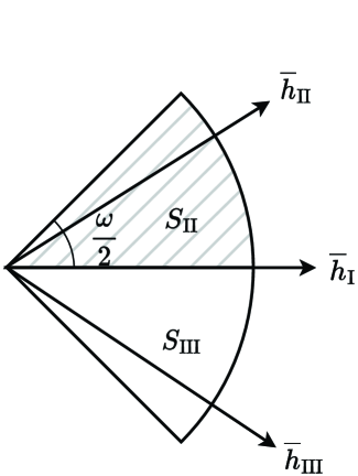
(a) 1st-time CSM

(b) 2nd-time CSM

Figure 3: Visualization of the procedure in Algorithm 2.

Algorithm 2 Grouped Conditional Sample Mean (GCSM)

1:input: $\Phi_{K}$ and $N$.

2:Divide the reflected channels into two groups $\mathcal{S}_{\mathrm{I}}$ and $\mathcal{S}^{c}_{\mathrm{I}}$.

3:for $t=1,2,\ldots,T_{1}$ do

4:     Fix $\mathcal{S}_{\mathrm{I}}$ and generate each $\theta_{nt}$ with $n\in\mathcal{S}^{c}_{\mathrm{I}}$ at random.

5:     Measure received signal power $\left|Y_{t}\right|^{2}$ under $\bm{\theta}_{t}$.

6:end for

7:1st round of CSM: Compute $\widehat{\mathbb{E}}\left[|Y|^{2}\mid\theta_{n}=k\omega\right]$ in (18) and decide $\theta_{n}$ for each RE in $\mathcal{S}^{c}_{\mathrm{I}}$ as in (19).

8:Further divide $\mathcal{S}^{c}_{\mathrm{I}}$ into $\mathcal{S}_{\mathrm{II}}$ and $\mathcal{S}_{\mathrm{III}}$ according to (26).

9:for $t=1,2,\ldots,T_{2}$ do

10:     Fix $\mathcal{S}_{\mathrm{II}}$ and generate each $\theta_{nt}$, $n\in\mathcal{S}_{\mathrm{I}}\cup\mathcal{S}_{\mathrm{III}}$ at random.

11:     Measure received signal power $\left|Y_{t}\right|^{2}$ under $\bm{\theta}_{t}$.

12:end for

13:2nd round of CSM: Compute $\widehat{\mathbb{E}}\left[|Y|^{2}\mid\theta_{n}=k\omega\right]$ in (18) and decide $\theta_{n}$ for each RE in $\mathcal{S}_{\mathrm{I}}$ and $S_{\mathrm{III}}$ as in (19);

Rather interestingly, we found that partitioning the set of REs into three groups can yield provable performance. First, divide the reflected channels $\left\{h_{1},\ldots,h_{N}\right\}$ into two groups $\mathcal{S}_{\mathrm{I}}$ and $\mathcal{S}^{c}_{\mathrm{I}}$. Fixing $\theta_{n}$ for $\mathcal{S}_{\mathrm{I}}$, we optimize $\theta_{n}$ in $\mathcal{S}^{c}_{\mathrm{I}}$ by CSM, i.e., the reflected channels in $\mathcal{S}_{\mathrm{I}}$ are now treated as parts of the virtual direct channel denoted by $h_{\mathrm{I}}$. With $h_{\mathrm{I}}$ being much stronger than $h_{0}$, CSM now works well. As a result, every $h_{n}\in\mathcal{S}^{c}_{\mathrm{I}}$ whose fixed part $\overline{h}_{n}$ would be rotated to the closest possible position to the $\overline{h}_{\mathrm{I}}$. Notice that the optimized fixed part of reflected channels must lie in the two sectors adjacent to $\overline{h}_{\mathrm{I}}$, both having an angle of $\omega/2$, as illustrated in Fig. 3(a).

We denote by $\mathcal{S}_{\mathrm{II}}\subseteq\mathcal{S}^{c}_{\mathrm{I}}$ the subset of optimized reflected channels whose fixed part lying in the upper sector (which is shaded in Fig. 3(a)), and $\mathcal{S}_{\mathrm{III}}\subseteq\mathcal{S}^{c}_{\mathrm{I}}$ the subset of optimized reflected channels whose fixed part lying in the lower sector. Moreover, we use $h_{\mathrm{II}}$ to denote the superposition of the channels in $\mathcal{S}_{\mathrm{II}}$, and $h_{\mathrm{III}}$ the superposition of the channels in $\mathcal{S}_{\mathrm{III}}$. The sequel shows that $\mathcal{S}_{\mathrm{II}}$ and $\mathcal{S}_{\mathrm{III}}$ can be determined by comparing $\hat{\mathbb{E}}\left[|Y|^{2}\mid\theta_{n}=\varphi\right]$. Consider an optimized reflected channel $h_{n}e^{j\theta_{n}}$ whose fixed part currently lies in the upper sector. Notice that $\overline{h}_{n}e^{j\left(\theta_{n}-\omega\right)}$ is closer to $\overline{h}_{\mathrm{I}}$ than $\overline{h}_{n}e^{j\left(\theta_{n}+\omega\right)}$ is, so $\hat{\mathbb{E}}\left[|Y|^{2}\mid\theta_{n}=\varphi-\omega\right]$ must be larger than $\hat{\mathbb{E}}\left[|Y|^{2}\mid\theta_{n}=\varphi+\omega\right]$. By symmetry, if $\overline{h}_{n}e^{j\theta_{n}}$ currently lies in the lower sector, we have $\hat{\mathbb{E}}\left[|Y|^{2}\mid\theta_{n}=\varphi+\omega\right]$ be larger than $\hat{\mathbb{E}}\left[|Y|^{2}\mid\theta_{n}=\varphi-\omega\right]$. In summary, we can tell which set each $h_{n}e^{j\theta_{n}}$ belongs to by comparing its associated conditional sample means, i.e.,

$$\hat{\mathbb{E}}[|Y|^{2}|\theta_{n}=\varphi+\omega]\underset{\mathcal{S}_{\mathrm{III}}}{\overset{\mathcal{S}_{\mathrm{II}}}{\lessgtr}}\hat{\mathbb{E}}[|Y|^{2}|\theta_{n}=\varphi-\omega].$$ (26)

The first stage of the proposed method is now completed. In the next stage, we fix $\theta_{n}$ for the reflected channels in $\mathcal{S}_{\mathrm{II}}$, and optimize those in $\mathcal{S}_{\mathrm{I}}$ and $\mathcal{S}_{\mathrm{III}}$ via CSM. The whole method is then completed. We summarize the above steps in Algorithm 2. The computational complexity of the algorithm is $O(N(T+K))$. Most importantly, the proposed method has provable performance, as stated in the following proposition.

Proposition 4

For the phase shift solution $\left\{\theta_{n}^{\mathrm{GCSM}}\right\}$ of Algorithm 2, there holds

$$\max_{a,b\in\{1,\ldots,N\}}\left|\angle\overline{h}_{a}+\theta_{a}^{\mathrm{GCSM}}-\angle\overline{h}_{b}-\theta_{b}^{\mathrm{GCSM}}\right|\leq\omega,$$ (27)

i.e., the fixed part of reflected channels are clustered inside a sector with an angle of $\omega$, so for the global optimum $f^{\star}$ the solution of Algorithm 2 guarantees

$$\cos^{2}(\frac{\pi}{K})\cdot f^{\star}\leq\mathbb{E}\left[\bigg{|}h_{0}+\sum_{n=1}^{N}h_{n}e^{j\theta_{n}^{\mathrm{GCSM}}}\bigg{|}^{2}\right]\leq f^{\star},$$ (28)

for the NLoS direct channel case with $\mathbb{E}[h_{0}]\rightarrow 0$.

Proof:

For the 1st-time CSM in Algorithm 2, all those fixed parts of reflected channels in $\mathcal{S}_{\mathrm{II}}$ are rotated to the closest possible position to the fixed part of current virtual direct channel $\overline{h}_{\mathrm{I}}$, so they must lie inside the shaded sector as shown in Fig. 3(a). Clearly, their superposition $\overline{h}_{\mathrm{II}}$ must lie in the shaded sector too. For the 2nd-time CSM, as shown in Fig. 3(b), all those fixed parts of reflected channels in $\mathcal{S}_{\mathrm{I}}$ and $\mathcal{S}_{\mathrm{III}}$ are rotated to the closest possible positions to $\overline{h}_{\mathrm{II}}$. Summarizing the above results gives (27). ∎

V Double-IRS Extension

We now consider extending our algorithm to a double-IRS network. The proposed extension looks fairly simple: just run CSM (or GCSM if the direct channel is NLoS) for each IRS one time, not even requiring iteration. But it is highly nontrivial to verify the performance of this simple method, as discussed in the second part of this section.

V-A Double-IRS System Model

Figure 4: Channel model of the double-IRS system.

For ease of notation, just assume that the two IRSs have the same number of REs $N$, and have the same discrete phase shift constraint $\Phi_{K}$; our method can be readily extended when $N$ or $\Phi_{K}$ differs between the two IRSs. The IRS closer to the transmitter is referred to as IRS 1, and the other is referred to as IRS 2. Use $n_{\ell}=1,\ldots,N$ to index each RE of IRS $\ell$, $\ell\in\{1,2\}$; use $\theta_{n_{\ell}}$ to denote the phase shift of RE $n_{\ell}$. Regarding the channels, we denote by $h_{n_{1}n_{2}}$ the reflected channel from the transmitter to RE $n_{1}$ of IRS 1 and then to RE $n_{2}$ of IRS 2 and ultimately to the receiver; let $n_{\ell}=0$ if the channel $h_{n_{1}n_{2}}$ is not related to IRS $\ell$; in particular, $h_{00}$ is the direct channel from the transmitter to the receiver.

We further discuss how each $h_{n_{1}n_{2}}$ is modeled. The direct channel is given by

$$h_{00}=\sqrt{\gamma_{00}}\left(\sqrt{\frac{\delta_{00}}{1+\delta_{00}}}\overline{h}_{00}+\sqrt{\frac{1}{1+\delta_{00}}}\widetilde{h}_{00}\right),$$ (29)

where $\gamma_{00}$ is the pathloss factor, $\delta_{00}$ is the Rician factor, $\overline{h}_{00}$ is a fixed normalized complex number, and $\widetilde{h}_{00}\sim\mathcal{CN}(0,1)$. Likewise, the channel from the transmitter to RE $n_{\ell}$ is given by

$$f_{n_{\ell}}=\sqrt{\gamma_{0n_{\ell}}}\left(\sqrt{\frac{\delta_{0n_{\ell}}}{1+\delta_{0n_{\ell}}}}\overline{f}_{n_{\ell}}+\sqrt{\frac{1}{1+\delta_{0n_{\ell}}}}\widetilde{f}_{n_{\ell}}\right),$$ (30)

the channel from RE $n_{\ell}$ to the receiver is given by

$$g_{n_{\ell}}=\sqrt{\gamma_{n_{\ell}0}}\left(\sqrt{\frac{\delta_{n_{\ell}0}}{1+\delta_{n_{\ell}0}}}\overline{g}_{n_{\ell}}+\sqrt{\frac{1}{1+\delta_{n_{\ell}0}}}\widetilde{g}_{n_{\ell}}\right),$$ (31)

and the channel from RE $n_{1}$ to RE $n_{2}$ is given by

$$q_{n_{1}n_{2}}=\sqrt{\gamma_{n_{1}n_{2}}}\left(\sqrt{\frac{\delta_{n_{1}n_{2}}}{1+\delta_{n_{1}n_{2}}}}\overline{q}_{n_{1}n_{2}}+\sqrt{\frac{1}{1+\delta_{n_{1}n_{2}}}}\widetilde{q}_{n_{1}n_{2}}\right),$$ (32)

where $\gamma_{0n_{\ell}}$, $\gamma_{n_{\ell}0}$, $\gamma_{n_{1}n_{2}}$ are the attenuation factors, $\delta_{0n_{\ell}}$, $\delta_{n_{\ell}0}$, $\delta_{n_{1}n_{2}}$ are the Rician factors, $\overline{f}_{n_{\ell}}$, $\overline{g}_{n_{\ell}}$, $\overline{q}_{n_{1}n_{2}}$ are fixed normalized complex numbers, and $\widetilde{f}_{n_{\ell}}$, $\widetilde{g}_{n_{\ell}}$, $\widetilde{q}_{n_{1}n_{2}}\sim\mathcal{CN}(0,1)$. As a result, each reflected channel amounts to a product of some of the above channels, i.e.,

$$h_{n_{1}n_{2}}=\begin{cases}f_{n_{1}}g_{n_{1}}&\text{if}\quad n_{1}\neq 0,\;n_{2}=0,\vspace{1ex}\\ f_{n_{2}}g_{n_{2}}&\text{if}\quad n_{1}=0,\;n_{2}\neq 0,\vspace{1ex}\\ f_{n_{1}}q_{n_{1}n_{2}}g_{n_{2}}&\text{if}\quad n_{1}\neq 0,\;n_{2}\neq 0.\vspace{1ex}\end{cases}$$ (33)

Summarizing (29) and (33), we can write each channel $h_{n_{1}n_{2}}$ in a uniform expression as

$$h_{n_{1}n_{2}}=\overline{\alpha}_{n_{1}n_{2}}\overline{h}_{n_{1}n_{2}}+\widetilde{\alpha}_{n_{1}n_{2}}\widetilde{h}_{n_{1}n_{2}}$$ (34)

where $\overline{h}_{n_{1}n_{2}}$ is a normalized complex constant (since a product of normalized complex numbers is still normalized), $\widetilde{h}_{n_{1}n_{2}}$ is a zero-mean random variable,

$$\overline{\alpha}_{n_{1}n_{2}}=\begin{cases}\sqrt{\frac{\gamma_{00}\delta_{00}}{1+\delta_{00}}}&n_{1}=n_{2}=0,\vspace{1ex}\\ \sqrt{\frac{\gamma_{0n_{1}}\gamma_{n_{1}0}\delta_{0n_{1}}\delta_{n_{1}0}}{(1+\delta_{0n_{1}})(1+\delta_{n_{1}0})}}&n_{2}=0,\vspace{1ex}\\ \sqrt{\frac{\gamma_{0n_{2}}\gamma_{n_{2}0}\delta_{0n_{2}}\delta_{n_{2}0}}{(1+\delta_{0n_{2}})(1+\delta_{n_{2}0})}}&n_{1}=0,\vspace{1ex}\\ \sqrt{\frac{\gamma_{0n_{1}}\gamma_{n_{1}n_{2}}\gamma_{n_{2}0}\delta_{0n_{1}}\delta_{n_{1}n_{2}}\delta_{n_{2}0}}{(1+\delta_{0n_{1}})(1+\delta_{n_{1}n_{2}})(1+\delta_{n_{2}0})}}\quad&n_{1}\neq 0,n_{2}\neq 0,\end{cases}$$ (35)

and

$$\widetilde{\alpha}_{n_{1}n_{2}}=\begin{cases}\sqrt{\frac{\gamma_{00}}{1+\delta_{00}}}&n_{1}=n_{2}=0,\vspace{1ex}\\ \sqrt{\frac{\gamma_{0n_{1}}\gamma_{n_{1}0}}{(1+\delta_{0n_{1}})(1+\delta_{n_{1}0})}}&n_{2}=0,\vspace{1ex}\\ \sqrt{\frac{\gamma_{0n_{2}}\gamma_{n_{2}0}}{(1+\delta_{0n_{2}})(1+\delta_{n_{2}0})}}&n_{1}=0,\vspace{1ex}\\ \sqrt{\frac{\gamma_{0n_{1}}\gamma_{n_{1}n_{2}}\gamma_{n_{2}0}}{(1+\delta_{0n_{1}})(1+\delta_{n_{1}n_{2}})(1+\delta_{n_{2}0})}}\quad&n_{1}\neq 0\text{ \& }n_{2}\neq 0.\end{cases}$$ (36)

We remark that the distribution function of each random variable $\widetilde{h}_{n_{1}n_{2}}$ can be obtained from (33)—which can be fairly complicated; fortunately, it is easy to see that each $\mathbb{E}[\widetilde{h}_{n_{1}n_{2}}]=0$ and this property is enough for our analysis later on.

Let $\theta_{n_{\ell}}$ be the phase shift of RE $n_{\ell}$. The overall expected channel power that we aim to maximize now becomes

$$\mathbb{E}\left[\Bigg{|}\sum^{N}_{n_{1}=0}\sum^{N}_{n_{2}=0}h_{n_{1}n_{2}}e^{j(\theta_{n_{1}}+\theta_{n_{2}})}\Bigg{|}^{2}\right],$$

where $\theta_{0}=0$ by convention. Accordingly, the optimizing variables in problem (9) are now $\{\theta_{n_{1}}\}$ and $\{\theta_{n_{2}}\}$.

V-B Sequential Blind Beamforming

Figure 5: Our field test uses an IRS that comprises 400 REs and provides 4 phase shift options $\{0,\pi/2,\pi,3\pi/2\}$ for each RE. For LoS direct channel case, omnidirectional antennas are deployed at both transmitter and receiver; for NLoS direct channel case, directional antennas are deployed to prevent direct signal propagation from transmitter to receiver.

The way we handle two IRSs is rather simple: first configure IRS 1 by CSM with IRS 2 held fixed, and then configure IRS 2 by CSM with IRS 1 held fixed, namely sequential CSM; CSM can be readily replaced with GCSM in each step if the NLoS direct channel case is encountered. Notably, this is not an iterative algorithm since each IRS is optimized only once.

It is tempting to think that a quartic boost of $\Theta(N^{4})$ can be always achieved for the channel power, claiming that IRS 1 first brings $N^{2}$ boost and then IRS 2 further brings $N^{2}$ boost according to Proposition 3. However, the above argument is problematic in that the quadratic boost by IRS 1 may no longer hold when IRS 2 has its phase shifts changed. The following example can illustrate this point well.

Example 1

Suppose that $h_{n_{1}n_{2}}=0$ whenever $n_{1}$ and $n_{2}$ are both nonzero, i.e., there does not exist any two-hop reflected channel; then the two IRSs can be thought of as a single IRS with $2N$ REs, and clearly the highest possible boost is $N^{2}$.

Actually, it requires some conditions for the sequential CSM algorithm to yield the $N^{4}$ boost, as stated in the following proposition.

Proposition 5

If $K>2$ and the channels of the double-IRS system satisfy the following conditions:

1. the two-hop channel matrix consisting of LoS channels is rank one and can be factorized as

   $$\begin{bmatrix}\overline{\alpha}_{11}\overline{h}_{11}&\ldots&\overline{\alpha}_{1N}\overline{h}_{1N}\\ \vdots&&\vdots\\ \overline{\alpha}_{N1}\overline{h}_{N1}&\ldots&\overline{\alpha}_{NN}\overline{h}_{NN}\end{bmatrix}=\begin{bmatrix}u^{(1)}_{1}\\ \vdots\\ u^{(1)}_{N}\end{bmatrix}\begin{bmatrix}u^{(2)}_{1}\ldots u^{(2)}_{N}\end{bmatrix},$$ (37)

2. there exists a constant $\zeta\in[0,\frac{\pi}{2}\!-\!\frac{\pi}{K})$ such that

   $$|\overline{\alpha}_{n_{1}0}\overline{h}_{n_{1}0}|\leq\sin\zeta\cdot\left|\sum^{N}_{n_{2}=1}\ \overline{\alpha}_{n_{1}n2}\overline{h}_{n_{1}n_{2}}\right|,\;\forall n_{1}\neq 0,$$ (38)

then the sequential CSM method yields

$$\mathbb{E}\left[\Bigg{|}\sum^{N}_{n_{1}=0}\sum^{N}_{n_{2}=0}h_{n_{1}n_{2}}e^{j(\theta_{n_{1}}+\theta_{n_{2}})}\Bigg{|}^{2}\right]=\Theta(N^{4})$$ (39)

as $T\rightarrow\infty$, where the expectation is taken over both random samples of $\bm{\theta}$ as well as random fading channels.

Proof:

Since there are a total of $N^{2}+2N+1$ channels from transmitter to receiver, we can readily see that the channel power is $O(N^{4})$.

We now verify the achievability. Every phase shift is initialized to zero. First, when IRS 2 is fixed, we use CSM to optimize each $\theta_{n_{1}}$; note that the current direct channel is $h_{0}^{\prime}=h_{00}+\sum^{N}_{n_{2}=1}h_{0n_{2}}$ while the current reflect channel of RE $n_{1}$ is $h_{n_{1}}^{\prime}=\sum^{N}_{n_{2}=0}h_{n_{1}n_{2}}$. Let $\Delta_{n_{1}}=\angle(\mathbb{E}[h_{0}^{\prime}])-\angle(\mathbb{E}[h_{n_{1}}^{\prime}])$. By Proposition 3, as $T\rightarrow\infty$, it holds that

$$\theta_{n_{1}}^{\mathrm{CSM}}=\arg\min_{\varphi\in\Phi_{K}}|\varphi-\Delta_{n_{1}}|.$$ (40)

And then we must have

$$|\theta_{n_{1}}^{\mathrm{CSM}}-\Delta_{n_{1}}|\leq\frac{\omega}{2}.$$ (41)

Moreover, we define

$$\hat{\theta}_{n_{1}}=\angle(\mathbb{E}[h_{0}^{\prime}])-\angle(u^{(1)}_{n_{1}})-\angle\left(\sum^{N}_{n_{2}=1}u^{(2)}_{n_{2}}\right).$$ (42)

By virtue of the conditions C1 and C2, we can show that

$$|\hat{\theta}_{n_{1}}-\Delta_{n_{1}}|\leq\zeta.$$ (43)

Combining (41) and (43) gives

$$|\hat{\theta}_{n_{1}}-\theta_{n_{1}}^{\mathrm{CSM}}|\leq\frac{\omega}{2}+\zeta.$$ (44)

The above inequality is crucial in the later part of the proof.

We now turn to the second stage in which IRS 1 is fixed while IRS 2 is optimized. Note that each $\theta_{n_{1}}$ has been updated to $\theta_{n_{1}}^{\mathrm{CSM}}$ at this point. Now, the current direct channel is $h_{0}^{\prime\prime}=h_{00}+\sum^{N}_{n_{1}=1}h_{n_{1}0}e^{j\theta_{n_{1}}^{\mathrm{CSM}}}$ while the current reflect channel of RE $n_{2}$ is $h_{n_{2}}^{\prime\prime}=h_{0n_{2}}+\sum^{N}_{n_{1}=1}h_{n_{1}n_{2}}e^{j\theta_{n_{1}}^{\mathrm{CSM}}}$. Accordingly, let $\Delta_{n_{2}}=\angle(\mathbb{E}[h_{0}^{\prime\prime}])-\angle(\mathbb{E}[h_{n_{2}}^{\prime\prime}])$. Repeating the steps in the previous stage, we obtain

$$\theta_{n_{2}}^{\mathrm{CSM}}=\arg\min_{\varphi\in\Phi_{K}}|\varphi-\Delta_{n_{2}}|$$ (45)

and

$$|\theta_{n_{2}}^{\mathrm{CSM}}-\Delta_{n_{2}}|\leq\frac{\omega}{2}.$$ (46)

Letting

$$\xi_{n_{2}}=\overline{\alpha}_{0n_{2}}\overline{h}_{0n_{2}}+\sum_{n_{1}=1}^{N}\overline{\alpha}_{n_{1}n_{2}}\overline{h}_{n_{1}n_{2}}e^{j\theta_{n_{1}}^{\mathrm{CSM}}},$$ (47)

it can be shown that

$$\mathbb{E}\left[\Bigg{|}\sum^{N}_{n_{1}=0}\sum^{N}_{n_{2}=0}h_{n_{1}n_{2}}e^{j(\theta^{\mathrm{CSM}}_{n_{1}}+\theta^{\mathrm{CSM}}_{n_{2}})}\Bigg{|}^{2}\right]$$

$$\geq\left|\overline{\alpha}_{00}\overline{h}_{00}+\sum_{n_{1}=1}^{N}\overline{\alpha}_{n_{1}0}\overline{h}_{n_{1}0}e^{j\theta_{n_{1}}^{\mathrm{CSM}}}+\sum_{n_{2}=1}^{N}\xi_{n_{2}}e^{j\theta_{n_{2}}^{\mathrm{CSM}}}\right|^{2}$$

$$\geq\cos^{2}(\frac{\omega}{2})\cdot\left(\sum_{n_{2}=1}^{N}|\xi_{n_{2}}|\right)^{2},$$ (48)

where the second inequality follows by (46). We further have

$$|\xi_{n_{2}}| =\left|\sum_{n_{1}=1}^{N}\overline{\alpha}_{n_{1}n_{2}}\overline{h}_{n_{1}n_{2}}e^{j\theta_{n_{1}}^{\mathrm{CSM}}}\right|+o(N)$$

$$=\left|\sum_{n_{1}=1}^{N}\overline{\alpha}_{n_{1}n_{2}}\overline{h}_{n_{1}n_{2}}e^{j\hat{\theta}_{n_{1}}}e^{j(\theta_{n_{1}}^{\mathrm{CSM}-\hat{\theta}_{n_{1}})}}\right|+o(N)$$

$$=|u_{n_{2}}^{(2)}|\cdot\left|\sum_{n_{1}=1}^{N}|u_{n_{1}}^{(1)}|e^{j(\theta_{n_{1}}^{\mathrm{CSM}}-\hat{\theta}_{n_{1}})}\right|+o(N)$$

$$\geq|u_{n_{2}}^{(2)}|\cdot\cos(\zeta+\frac{\omega}{2})\cdot\sum_{n_{1}=1}^{N}|u_{n_{1}}^{(1)}|+o(N),$$ (49)

where the last step is due to (44). Finally, combining (48) and (49) gives rise to

$$\mathbb{E}\left[\Bigg{|}\sum^{N}_{n_{1}=0}\sum^{N}_{n_{2}=0}h_{n_{1}n_{2}}e^{j(\theta^{\mathrm{CSM}}_{n_{1}}+\theta^{\mathrm{CSM}}_{n_{2}})}\Bigg{|}^{2}\right]$$

$$=\Omega\left(\left(\sum_{n_{2}=1}^{N}\sum_{n_{2}=1}^{N}|u_{n_{1}}^{(1)}||u_{n_{2}}^{(2)}|\right)^{2}\right)$$

$$=\Omega(N^{4}).$$ (50)

Since the expected power of the overall channel is both $O(N^{4})$ and $\Omega(N^{4})$, it must be $\Theta(N^{4})$. ∎

Figure 6: Layout drawing of our field test.

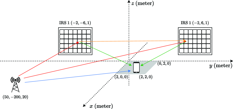
Figure 7: The double-IRS system considered in our simulations. The receiver is randomly located within the shaded area.

VI Numerical results

VI-A Field Tests

We carry out the field test in an outdoor environment as shown in Fig. 5; the corresponding layout drawing is depicted in Fig. 6. Throughout the field test, the transmit power is fixed to be $-10$ dBm and the transmission takes place at $3.5$ GHz. The IRS prototype machine consists of $400$ REs (i.e., $N=400$) and provides 4 possible phase shifts $\{0,\pi/2,\pi,3\pi/2\}$ for each RE. For LoS direct channel case, omnidirectional antennas are deployed at both transmitter and receiver; for NLoS direct channel case, directional antennas are deployed to prevent direct signal propagation from transmitter to receiver. Aside from the CSM method in Algorithm 1 and the GCSM method in Algorithm 2, the following methods are included in field tests as benchmarks:

• IRS Removed (RMV): IRS is removed from the network.

• Zero Phase Shifts (ZPS): Fix all phase shifts to be zero.

• Random Max Sampling (RMS): Try out $T$ random samples of $\bm{\theta}$ and choose the best.

Notice that RMS, CSM, and GCSM all require random samples of $\bm{\theta}$. For fairness, the same random sample size $T=1000$ is used for them.

TABLE I summarizes the performance of the different IRS beamforming algorithms. Observe that the ZPS method increases SNR significantly by 23.8 dB for the NLoS direct channel case even with the phase shifts all fixed at zero, whereas its gain is marginal (only 1.8 dB) for the LoS case. Observe also that RMS increases SNR further by about 8 dB as compared to ZPS, at the cost of 1000 random samples. Thus, the deployment of IRS can already bring considerable gain even without any phase shift optimization if the original channel is too bad.

But the much higher gain can be reaped by using more sophisticated algorithms like CSM and GCSM. The table shows that CSM can further improve upon RMS by around 7 dB in the LoS case; we remark that CSM uses the same number of random samples as RMS does, and that its computational complexity is not higher. Notice that the gap between CSM and GCSM is slim in the LoS case as expected. But when it comes to the NLoS case, GCSM starts to outperform: SNR of GCSM is 2.4 dB higher than that of CSM. We also notice that the advantage of CSM over RMS shrinks in the NLoS case. But since the two algorithms require similar sampling and computation costs, the former is still preferable in practice.

TABLE I: Performance of the Different Algorithms in LoS and NLoS Direct Channel Cases

	LoS		NLoS
Method	SNR (dB)	Boost (dB)	SNR (dB)	Boost (dB)
RMV	8.5	0.0	3.0	0.0
ZPS	10.3	1.8	26.8	23.8
RMS	17.7	9.2	35.7	32.7
CSM	24.4	15.9	29.2	36.7
GCSM	24.8	16.3	42.1	39.1

VI-B Simulations

We now consider simulations to validate the performance of the proposed blind beamforming method under more complex network settings, i.e., with two IRSs and with many more REs on each IRS.

As shown in Fig. 7, we consider a double-IRS system. The REs are arranged as a half-wavelength spaced uniform linear array (ULA); the carrier frequency equals 2.6 GHz, so the wavelength $\lambda\approx 10$ cm and thus the RE spacing equals 5 cm. We now specify the model parameters in Section V-A. The pathloss factors are generated as

$$-10\cdot\log_{10}\gamma_{00} =32.6+36.7\log_{10}(d_{00}),$$ (51a)

$$-10\cdot\log_{10}\gamma_{0n_{\ell}} =30+22\log_{10}(d_{0n_{\ell}}),$$ (51b)

$$-10\cdot\log_{10}\gamma_{n_{\ell}0} =30+22\log_{10}(d_{n_{\ell}0}),$$ (51c)

$$-10\cdot\log_{10}\gamma_{n_{1}n_{2}} =30+22\log_{10}(d_{n_{1}n_{2}}),$$ (51d)

where $d_{00}$, $d_{0n_{\ell}}$, $d_{n_{\ell}0}$, and $d_{n_{1}n_{2}}$ are the corresponding distance in meters. Moreover, the normalized fixed components are generated as

$$\overline{h}_{00} =\exp\left(-j\frac{2\pi d_{00}}{\lambda}\right),$$ (52a)

$$\overline{f}_{n_{\ell}} =\exp\left(-j\frac{2\pi d_{0n_{\ell}}}{\lambda}\right),$$ (52b)

$$\overline{g}_{n_{\ell}} =\exp\left(-j\frac{2\pi d_{n_{\ell}0}}{\lambda}\right),$$ (52c)

$$\overline{q}_{n_{1}n_{2}} =\exp\left(-j\frac{2\pi d_{n_{1}n_{2}}}{\lambda}\right).$$ (52d)

Regarding the Rician factors, we let $\delta_{0n_{\ell}}=\delta_{n_{\ell}0}=\delta_{n_{1}n_{2}}=10$; the value of $\delta_{00}$ depends on the direct channel status—let $\delta_{00}=10$ for the LoS case and let $\delta_{00}=0$ for the NLoS case.

The rest parameters are set as follows unless otherwise stated. The transmit power level $P=20$ dBm, and the background noise power level $\sigma^{2}=-90$ dBm. Assume that IRS 1 and IRS 2 have $N=100$ REs each; but we will test different values of $N$ later on. The number of phase shift choices $K$ is fixed to be 4. The sample size $T=1000$ by default; but we will change $T$ to see how it impacts the performance of blind beamforming. We evaluate the ergodic data rate by averaging out $10000$ realizations of fading channels.

Aside from CSM, GCSM, and RMS (see the previous subsection), the following baseline methods are considered:

• Perfect CSI: Perform the closest point projection in (12) for the two IRSs sequentially; we remark that CSM or GCSM converges to this scheme if $T\rightarrow\infty$.

• Estimated CSI: Follow the above baseline method except that CSI is estimated by the DFT method [25].

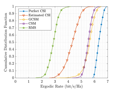
Figure 8: Cumulative distributions of ergodic rates in the LoS case.

Let us begin with the single-IRS case in which only IRS 1 is deployed while IRS 2 is removed. The resulting cumulative distributions of ergodic data rates achieved by the different algorithms in the LoS direct channel case are displayed in Fig. 8. It can be seen that the proposed blind beamforming method CSM outperforms the estimated CSI method and the RMS method significantly. For instance, CSM improves upon RMS by about 30% and upon GCSM by about 90% at the 50th percentile. Observe that CSM and GCSM yield similar performance for the LoS case in Fig. 8. By contrast, as shown in Fig. 9, GCSM is far superior to CSM when the direct channel becomes NLoS. Actually, CSM is the worst among all competitor algorithms in the NLoS case. Fig. 8 and Fig. 9 also show that GCSM is quite close to perfect CSI (which amounts to GCSM with infinitely many samples); thus, using merely $T=1000$ samples is good enough in this case.

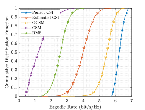
Figure 9: Cumulative distributions of ergodic rates in the NLoS case.

It is worthwhile to look into the NLoS case more closely by comparing the phase shift decisions of the different methods. Fig. 10 shows how the reflected channels are rotated in the complex plane by the phase shifts of the different methods. The results here are consistent with what we have observed in Fig. 9. The perfect CSI method renders the reflected channels most clustered and hence yields the highest SNR boost. GCSM with $T=1000$ also leads to most channels being clustered within an angle of $\pi/2$, albeit a few reflected channels deviate from the main beam because of the limited samples. In comparison, the estimated CSI method results in the reflected channels being more dispersed, and accordingly its performance is indeed worse than the previous two methods. Notably, CSM has the reflected channels be uniformly distributed, so it ends up with the worst performance.

We further consider how the SNR boost of blind beamforming scales with the number of REs $N$. The receiver position is now fixed at the origin point as shown in Fig. 7. Fig. 11 compares the SNR boost versus $N$ performance in the LoS case; we test RMS as well as CSM with different $T$ values. In particular, we remark that CSM with $T\rightarrow\infty$ is equivalent to the perfect CSI method. As shown in Fig. 11, the SNR boost brought by RMS is approximately linear in $N$, while the rest algorithms yield faster growths of SNR boost in $N$—which are quasi-quadratic. Actually, with $T=KN^{2}$, CSM can almost reach its ideal status with infinitely many samples. Moreover, we can make a similar observation about the NLoS case from Fig. 12.

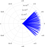
(a) Perfect CSI

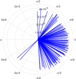
(b) Estimated CSI

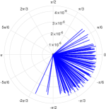
(c) GCSM

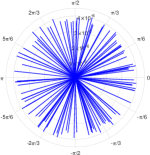
(d) CSM

Figure 10: The phase shifted channels $\overline{h}_{n}e^{j\theta_{n}}$ in the complex plane by the different IRS beamforming methods.

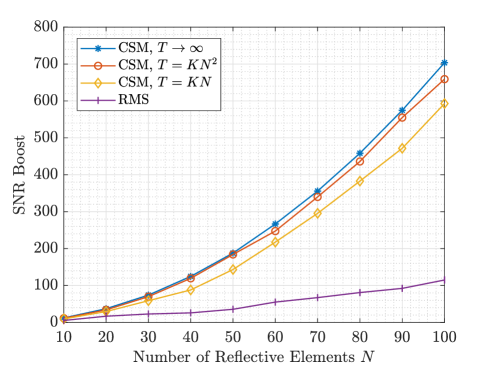
Figure 11: SNR boost versus $N$ in the LoS case.

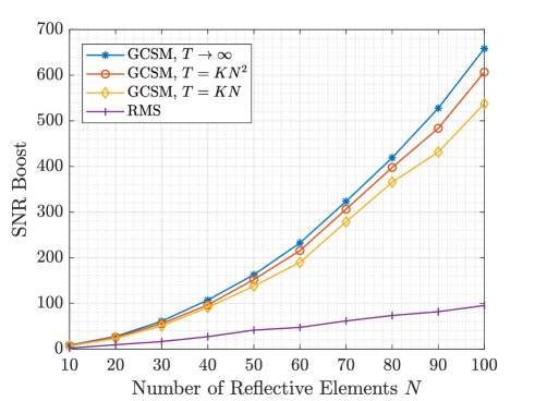
Figure 12: SNR boost versus $N$ in the NLoS case.

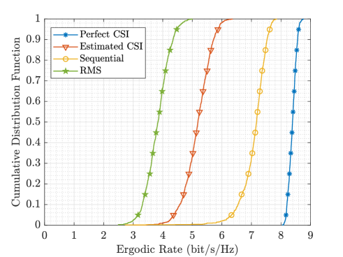
Figure 13: Cumulative distributions of ergodic rate in the double-IRS system.

Figure 14: SNR boost versus $N$ in the double-IRS system.

Finally, we validate the performance of blind beamforming in a double-IRS system. The two IRSs are placed as in Fig. 7. Notice that the LoS direct channel condition always holds in this case, so the sequential CSM method is used here. First, Fig. 13 compares the cumulative distributions of ergodic rate of the different methods. Observe that the sequential CSM has a huge advantage over RMS and estimated CSI. For instance, in the 50th percentile, the sequential CSM increases the ergodic rate of RMS by about 90% and increases that of the estimated CSI by about 40%. Observe also that the sequential CSM can bring further gain if many more samples are provided—it will ultimately converge to the perfect CSI when $T\rightarrow\infty$. Moreover, as shown in Fig. 14, the growth curve of the SNR boost versus $N$ resembles that in the single-IRS case, only that the gap between blind beamforming and RMS now becomes even larger. The above result agrees with the preceding analysis in Proposition 5 that the SNR boost by the sequential CSM grows exponentially with the number of IRSs.

VII Conclusion

This work advocates a blind beamforming approach to the phase shift optimization problem of IRS without requiring any channel estimation. Although the idea of blind beamforming has been considered in the recent works [28, 62, 63], their discussions are all restricted to fixed channels, whereas this work extends blind beamforming to fading channels. We first show that the proposed CSM algorithm guarantees a quadratic boost of SNR for fading channels so long as the direct link is LoS. Nevertheless, if the direct link is NLoS, then there is a subtle issue that can completely jeopardize the CSM algorithm. To address this issue, we suggest dividing all the REs into three groups and performing CSM for them separately. Furthermore, we extend the proposed algorithm to the double-IRS system and establish its optimality under certain conditions. All the above results are numerically verified in the field tests and simulations. Indeed, the proposed blind beamforming algorithm enables a fast configuration of IRS in a plug-and-play fashion, while not compromising its performance whatsoever.

References

• [1] B. Zheng, C. You, W. Mei, and R. Zhang, “A survey on channel estimation and practical passive beamforming design for intelligent reflecting surface aided wireless communications,” IEEE Commun. Surveys Tuts., vol. 24, no. 2, pp. 1035–1071, Feb. 2022.
• [2] Q. Wu and R. Zhang, “Intelligent reflecting surface enhanced wireless network via joint active and passive beamforming,” IEEE Trans. Wireless Commun., vol. 18, no. 11, pp. 5394–5409, Nov. 2019.
• [3] B. Zheng, C. You, and R. Zhang, “Double-IRS assisted multi-user MIMO: Cooperative passive beamforming design,” IEEE Trans. Wireless Commun., vol. 20, no. 7, pp. 4513–4526, Jul. 2021.
• [4] G. Zhou, C. Pan, H. Ren, K. Wang, M. Di Renzo, and A. Nallanathan, “Robust beamforming design for intelligent reflecting surface aided MISO communication systems,” IEEE Wireless Commun. Lett., vol. 9, no. 10, pp. 1658–1662, Jun. 2020.
• [5] M. Zeng, X. Li, G. Li, W. Hao, and O. A. Dobre, “Sum rate maximization for IRS-assisted uplink NOMA,” IEEE Commun. Lett., vol. 25, no. 1, pp. 234–238, Jan. 2020.
• [6] H. Xie, J. Xu, and Y.-F. Liu, “Max-min fairness in IRS-aided multi-cell MISO systems with joint transmit and reflective beamforming,” IEEE Trans. Wireless Commun., vol. 20, no. 2, pp. 1379–1393, Feb. 2020.
• [7] S. Huang, Y. Ye, M. Xiao, H. V. Poor, and M. Skoglund, “Decentralized beamforming design for intelligent reflecting surface-enhanced cell-free networks,” IEEE Wireless Commun. Lett., vol. 10, no. 3, pp. 673–677, Jun. 2020.
• [8] D. Mishra and H. Johansson, “Channel estimation and low-complexity beamforming design for passive intelligent surface assisted MISO wireless energy transfer,” in IEEE Int. Conf. Acoust. Speech Signal Process. (ICASSP), May 2019, pp. 4659–4663.
• [9] Z.-Q. Luo, W.-K. Ma, A. M.-C. So, Y. Ye, and S. Zhang, “Semidefinite relaxation of quadratic optimization problems,” IEEE Signal Process. Mag., vol. 27, no. 3, pp. 20–34, Apr. 2010.
• [10] K. Feng, X. Li, Y. Han, S. Jin, and Y. Chen, “Physical layer security enhancement exploiting intelligent reflecting surface,” IEEE Commun. Lett., vol. 25, no. 3, pp. 734–738, Mar. 2020.
• [11] J. Zhu, Y. Huang, J. Wang, K. Navaie, and Z. Ding, “Power efficient IRS-assisted NOMA,” IEEE Trans. Commun., vol. 69, no. 2, pp. 900–913, Feb. 2020.
• [12] T. Shafique, H. Tabassum, and E. Hossain, “Optimization of wireless relaying with flexible UAV-borne reflecting surfaces,” IEEE Trans. Commun., vol. 69, no. 1, pp. 309–325, Jan. 2020.
• [13] Z. Zhang, L. Dai, X. Chen, C. Liu, F. Yang, R. Schober, and H. V. Poor, “Active RIS vs. passive RIS: Which will prevail in 6G?” IEEE Trans. Commun., vol. 71, no. 3, pp. 1707–1725, Mar. 2022.
• [14] Z. Zhang and L. Dai, “A joint precoding framework for wideband reconfigurable intelligent surface-aided cell-free network,” IEEE Trans. Signal Process., vol. 69, pp. 4085–4101, Jun. 2021.
• [15] K. Shen and W. Yu, “Fractional programming for communication systems—part I: Power control and beamforming,” IEEE Trans. Signal Process., vol. 66, no. 10, pp. 2616–2630, May 2018.
• [16] ——, “Fractional programming for communication systems—part II: Uplink scheduling via matching,” IEEE Trans. Signal Process., vol. 66, no. 10, pp. 2631–2644, May 2018.
• [17] C. Huang, A. Zappone, G. C. Alexandropoulos, M. Debbah, and C. Yuen, “Reconfigurable intelligent surfaces for energy efficiency in wireless communication,” IEEE Trans. Wireless Commun., vol. 18, no. 8, pp. 4157–4170, Aug. 2019.
• [18] H. Shen, W. Xu, S. Gong, C. Zhao, and D. W. K. Ng, “Beamforming optimization for IRS-aided communications with transceiver hardware impairments,” IEEE Trans. Commun., vol. 69, no. 2, pp. 1214–1227, Feb. 2020.
• [19] Y. Sun, P. Babu, and D. P. Palomar, “Majorization-minimization algorithms in signal processing, communications, and machine learning,” IEEE Trans. Signal Process., vol. 65, no. 3, pp. 794–816, Feb. 2016.
• [20] Q. Wu and R. Zhang, “Beamforming optimization for wireless network aided by intelligent reflecting surface with discrete phase shifts,” IEEE Trans. Commun., vol. 68, no. 3, pp. 1838–1851, Mar. 2020.
• [21] Y. Li, M. Jiang, Q. Zhang, and J. Qin, “Joint beamforming design in multi-cluster MISO NOMA reconfigurable intelligent surface-aided downlink communication networks,” IEEE Trans. Commun., vol. 69, no. 1, pp. 664–674, Jan. 2021.
• [22] M.-M. Zhao, Q. Wu, M.-J. Zhao, and R. Zhang, “Intelligent reflecting surface enhanced wireless networks: Two-timescale beamforming optimization,” IEEE Trans. Wireless Commun., vol. 20, no. 1, pp. 2–17, Jan. 2020.
• [23] Y. Yang, B. Zheng, S. Zhang, and R. Zhang, “Intelligent reflecting surface meets OFDM: Protocol design and rate maximization,” IEEE Trans. Commun., vol. 68, no. 7, pp. 4522–4535, Jul. 2020.
• [24] S. Lin, B. Zheng, G. C. Alexandropoulos, M. Wen, M. Di Renzo, and F. Chen, “Reconfigurable intelligent surfaces with reflection pattern modulation: Beamforming design and performance analysis,” IEEE Trans. Wireless Commun., vol. 20, no. 2, pp. 741–754, Feb. 2021.
• [25] B. Zheng and R. Zhang, “Intelligent reflecting surface-enhanced OFDM: Channel estimation and reflection optimization,” IEEE Wireless Commun. Lett., vol. 9, no. 4, pp. 518–522, Apr. 2019.
• [26] T. L. Jensen and E. De Carvalho, “An optimal channel estimation scheme for intelligent reflecting surfaces based on a minimum variance unbiased estimator,” in IEEE Int. Conf. Acoust. Speech Signal Process. (ICASSP), May 2020.
• [27] G. T. de Araújo, A. L. De Almeida, and R. Boyer, “Channel estimation for intelligent reflecting surface assisted mimo systems: A tensor modeling approach,” IEEE J. Sel. Areas Commun., vol. 15, no. 3, pp. 789–802, Apr. 2021.
• [28] V. Arun and H. Balakrishnan, “RFocus: beamforming using thousands of passive antennas,” in USENIX Symp. Netw. Sys. Design Implementation (NSDI), Feb. 2020, pp. 1047–1061.
• [29] X. Pei, H. Yin, L. Tan, L. Cao, Z. Li, K. Wang, K. Zhang, and E. Björnson, “RIS-aided wireless communications: Prototyping, adaptive beamforming, and indoor/outdoor field trials,” IEEE Trans. Commun., vol. 69, no. 12, pp. 8627–8640, Dec. 2021.
• [30] N. M. Tran, M. M. Amri, D. S. Kang, J. H. Park, M. H. Lee, D. I. Kim, and K. W. Choi, “Demonstration of reconfigurable metasurface for wireless communications,” in IEEE Wireless Commun. Netw. Conf. Workshops (WCNC Workshops), Apr. 2020.
• [31] P. Staat, S. Mulzer, S. Roth, V. Moonsamy, M. Heinrichs, R. Kronberger, A. Sezgin, and C. Paar, “IRShield: A countermeasure against adversarial physical-layer wireless sensing,” in IEEE Symp. Secur. Priv. (SP), May 2022.
• [32] H. Ren, C. Pan, L. Wang, W. Liu, Z. Kou, and K. Wang, “Long-term CSI-based design for RIS-aided multiuser MISO systems exploiting deep reinforcement learning,” IEEE Commun. Lett., vol. 26, no. 3, pp. 567–571, Mar. 2022.
• [33] X. Gan, C. Zhong, C. Huang, and Z. Zhang, “RIS-assisted multi-user MISO communications exploiting statistical CSI,” IEEE Trans. Commun., vol. 69, no. 10, pp. 6781–6792, Oct. 2021.
• [34] M. Eskandari, H. Zhu, A. Shojaeifard, and J. Wang, “Statistical CSI-based beamforming for RIS-aided multiuser MISO systems using deep reinforcement learning,” 2022, [Online]. Available: https://arxiv.org/abs/2209.09856.
• [35] Y. Han, W. Tang, S. Jin, C.-K. Wen, and X. Ma, “Large intelligent surface-assisted wireless communication exploiting statistical CSI,” IEEE Trans. Veh. Technol., vol. 68, no. 8, pp. 8238–8242, Aug. 2019.
• [36] Y. Jia, C. Ye, and Y. Cui, “Analysis and optimization of an intelligent reflecting surface-assisted system with interference,” IEEE Trans. Wireless Commun., vol. 19, no. 12, pp. 8068–8082, Dec. 2020.
• [37] Y. Gao, J. Xu, W. Xu, D. W. K. Ng, and M.-S. Alouini, “Distributed IRS with statistical passive beamforming for MISO communications,” IEEE Wireless Commun. Lett., vol. 10, no. 2, pp. 221–225, Feb. 2020.
• [38] Z. Peng, T. Li, C. Pan, H. Ren, W. Xu, and M. Di Renzo, “Analysis and optimization for RIS-aided multi-pair communications relying on statistical CSI,” IEEE Trans. Veh. Technol., vol. 70, no. 4, pp. 3897–3901, Apr. 2021.
• [39] J. Wang, H. Wang, Y. Han, S. Jin, and X. Li, “Joint transmit beamforming and phase shift design for reconfigurable intelligent surface assisted MIMO systems,” IEEE Trans. on Cogn. Commun. Netw., vol. 7, no. 2, pp. 354–368, Jun. 2021.
• [40] K. Xu, J. Zhang, X. Yang, S. Ma, and G. Yang, “On the sum-rate of RIS-assisted MIMO multiple-access channels over spatially correlated Rician fading,” IEEE Trans. Commun., vol. 69, no. 12, pp. 8228–8241, Dec. 2021.
• [41] J. Dai, F. Zhu, C. Pan, H. Ren, and K. Wang, “Statistical CSI-based transmission design for reconfigurable intelligent surface-aided massive MIMO systems with hardware impairments,” IEEE Wireless Commun. Lett., vol. 11, no. 1, pp. 38–42, Jan. 2021.
• [42] G. Hu, J. Si, Y. Cai, and N. Al-Dhahir, “Intelligent reflecting surface-assisted proactive eavesdropping over suspicious broadcasting communication with statistical CSI,” IEEE Trans. Veh. Technol., vol. 71, no. 4, pp. 4483–4488, Apr. 2022.
• [43] K. Zhi, C. Pan, H. Ren, and K. Wang, “Power scaling law analysis and phase shift optimization of RIS-aided massive MIMO systems with statistical CSI,” IEEE Trans. Commun., vol. 70, no. 5, pp. 3558–3574, May 2022.
• [44] Z. Kang, C. You, and R. Zhang, “Active-passive IRS aided wireless communication: New hybrid architecture and elements allocation optimization,” 2022, [Online]. Available: https://arxiv.org/abs/2207.01244.
• [45] L. Jiang, C. Luo, X. Li, M. Matthaiou, and S. Jin, “RIS-assisted downlink multi-cell communication using statistical CSI,” in 2022 International Symposium on Wireless Communication Systems (ISWCS), Oct. 2022, pp. 1–6.
• [46] A. Papazafeiropoulos, C. Pan, A. Elbir, P. Kourtessis, S. Chatzinotas, and J. M. Senior, “Coverage probability of distributed IRS systems under spatially correlated channels,” IEEE Wireless Commun. Lett., vol. 10, no. 8, pp. 1722–1726, Aug. 2021.
• [47] T. Van Chien, A. K. Papazafeiropoulos, L. T. Tu, R. Chopra, S. Chatzinotas, and B. Ottersten, “Outage probability analysis of IRS-assisted systems under spatially correlated channels,” IEEE Wireless Commun. Lett., vol. 10, no. 8, pp. 1815–1819, Aug. 2021.
• [48] L. You, J. Xiong, Y. Huang, D. W. K. Ng, C. Pan, W. Wang, and X. Gao, “Reconfigurable intelligent surfaces-assisted multiuser MIMO uplink transmission with partial CSI,” IEEE Trans. Wireless Commun., vol. 20, no. 9, pp. 5613–5627, Sep. 2021.
• [49] A. P. Ajayan, S. P. Dash, and B. Ramkumar, “Performance analysis of an IRS-aided wireless communication system with spatially correlated channels,” IEEE Wireless Commun. Lett., vol. 11, no. 3, pp. 563–567, Mar. 2021.
• [50] H. Zhang, S. Ma, Z. Shi, X. Zhao, and G. Yang, “Sum-rate maximization of RIS-aided multi-user MIMO systems with statistical CSI,” IEEE Trans. Wireless Commun., 2022, to be published.
• [51] X. Zhang, X. Yu, S. Song, and K. B. Letaief, “IRS-aided MIMO systems over double-scattering channels: Impact of channel rank deficiency,” in Proc. IEEE Wireless Commun. Netw. Conf. (WCNC), Apr. 2022.
• [52] L. Yuan, Q. Du, N. Yang, and F. Fang, “Performance analysis of IRS-aided short-packet NOMA systems over nakagami-$m$ fading channels,” IEEE Trans. Veh. Technol., 2023, to be published.
• [53] X. Liu, B. Zhao, M. Lin, J. Ouyang, J.-B. Wang, and J. Wang, “IRS-aided uplink transmission scheme in integrated satellite-terrestrial networks,” IEEE Trans. Veh. Technol., vol. 72, no. 2, pp. 1847–1861, Feb. 2023.
• [54] J. Zhang, J. Liu, S. Ma, C.-K. Wen, and S. Jin, “Large system achievable rate analysis of RIS-assisted MIMO wireless communication with statistical CSIT,” IEEE Trans. Wireless Commun., vol. 20, no. 9, pp. 5572–5585, Sep. 2021.
• [55] C. Luo, X. Li, S. Jin, and Y. Chen, “Reconfigurable intelligent surface-assisted multi-cell MISO communication systems exploiting statistical CSI,” IEEE Wireless Commun. Lett., vol. 10, no. 10, pp. 2313–2317, Oct. 2021.
• [56] Y. Cao, T. Lv, and W. Ni, “Two-timescale optimization for intelligent reflecting surface-assisted MIMO transmission in fast-changing channels,” IEEE Trans. Wireless Commun., vol. 21, no. 12, pp. 10 424–10 437, Dec. 2022.
• [57] S. Shekhar, A. Subhash, T. Kella, and S. Kalyani, “Instantaneous channel oblivious phase shift design for an IRS-assisted SIMO system with quantized phase shift,” 2022, [Online]. Available: https://arxiv.org/abs/2211.03317.
• [58] Z. Zhang, T. Jiang, and W. Yu, “Learning based user scheduling in reconfigurable intelligent surface assisted multiuser downlink,” IEEE J. Sel. Topics Signal Process., vol. 16, no. 5, pp. 1026–1039, Aug. 2022.
• [59] H. Guo, Y.-C. Liang, and S. Xiao, “Intelligent reflecting surface configuration with historical channel observations,” IEEE Wireless Commun. Lett., vol. 9, no. 11, pp. 1821–1824, Nov. 2020.
• [60] Q.-U.-A. Nadeem, A. Zappone, and A. Chaaban, “Intelligent reflecting surface enabled random rotations scheme for the MISO broadcast channel,” IEEE Trans. Wireless Commun., vol. 20, no. 8, pp. 5226–5242, Aug. 2021.
• [61] C. Psomas and I. Krikidis, “Low-complexity random rotation-based schemes for intelligent reflecting surfaces,” IEEE Trans. Wireless Commun., vol. 20, no. 8, pp. 5212–5225, Aug. 2021.
• [62] S. Ren, K. Shen, Y. Zhang, X. Li, X. Chen, and Z.-Q. Luo, “Configuring intelligent reflecting surface with performance guarantees: Blind beamforming,” IEEE Trans. Wireless Commun., vol. 22, no. 5, pp. 3355–3370, May 2023.
• [63] F. Xu, J. Yao, W. Lai, K. Shen, X. Li, X. Chen, and Z.-Q. Luo, “Coordinating multiple intelligent reflecting surfaces without channel information,” 2023, [Online]. Available: https://arxiv.org/abs/2302.09717.
• [64] A. Goldsmith, Wireless communications.   Cambridge university press, 2005.
• [65] S. Ren, K. Shen, X. Li, X. Chen, and Z.-Q. Luo, “A linear time algorithm for the optimal discrete IRS beamforming,” IEEE Wireless Commun. Lett., vol. 12, no. 3, pp. 496–500, Mar. 2022.