Robust mean change point testing in high-dimensional data with heavy tails

Abstract

We study a mean change point testing problem for high-dimensional data, with exponentially- or polynomially-decaying tails. In each case, depending on the $\ell_{0}$-norm of the mean change vector, we separately consider dense and sparse regimes. We characterise the boundary between the dense and sparse regimes under the above two tail conditions for the first time in the change point literature and propose novel testing procedures that attain optimal rates in each of the four regimes up to a poly-iterated logarithmic factor. By comparing with previous results under Gaussian assumptions, our results quantify the costs of heavy-tailedness on the fundamental difficulty of change point testing problems for high-dimensional data.

To be specific, when the error vectors follow sub-Weibull distributions, a CUSUM-type statistic is shown to achieve a minimax testing rate up to $\sqrt{\log\log(8n)}$. When the error distributions have polynomially-decaying tails, admitting bounded $\alpha$-th moments for some $\alpha\geq 4$, we introduce a median-of-means-type test statistic that achieves a near-optimal testing rate in both dense and sparse regimes. In particular, in the sparse regime, we further propose a computationally-efficient test to achieve the exact optimality. Surprisingly, our investigation in the even more challenging case of $2\leq\alpha<4$, unveils a new phenomenon that the minimax testing rate has no sparse regime, i.e. testing sparse changes is information-theoretically as hard as testing dense changes. This phenomenon implies a phase transition of the minimax testing rates at $\alpha=4$.

1 Introduction

In this paper, we study the single change point testing problem when the observations are corrupted by heavy-tailed errors. To be specific, consider the ‘signal plus noise’ model

$$X=\theta+E,$$ (1)

where $X$, $\theta$ and $E$ are all $p\times n$ matrices, and the entries of $E$ are independent random variables with zero mean and unit variance. We denote the distribution of $E$ as $P_{e}\in\mathcal{Q}$. We are interested in understanding the fundamental difficulty of testing whether the columns of $\theta$ undergo a change at some unknown location when the class $\mathcal{Q}$ contains heavy-tailed distributions. By writing $\theta_{t}$ as the $t$-th column of $\theta$, our goal can be formalised as testing

$$\mathrm{H}_{0}:\theta\in\Theta_{0}(p,n)\quad\mathrm{vs.}~{}\quad\mathrm{H}_{1}:\theta\in\Theta(p,n,s,\rho):=\bigcup_{t_{0}=1}^{n-1}\Theta^{(t_{0})}(p,n,s,\rho),$$ (2)

where

$$\Theta_{0}(p,n):=\{ \theta:\theta_{t}=\mu\ \text{for all}\ t=1,2,\dotsc,n,\ \text{for some}\ \mu\in\mathbb{R}^{p}\}$$

and

$$\Theta^{(t_{0})}(p,n,s,\rho):=\biggl{\{} \theta:\theta_{t}=\mu_{1}\ \text{for}\ t=1,\ldots,t_{0},\ \theta_{t}=\mu_{2}\ \text{for}\ t=t_{0}+1,\ldots,n,$$

$$\text{for some}\ \mu_{1},\mu_{2}\in\mathbb{R}^{p}\ \text{s.t.}\ \|\mu_{1}-\mu_{2}\|_{0}\leq s,\,\frac{t_{0}(n-t_{0})}{n}\|\mu_{1}-\mu_{2}\|_{2}^{2}\geq\rho^{2}\biggr{\}}.$$

To put it in words, we use $\Theta_{0}(p,n)$ to denote the space of signals without a change point, and $\Theta^{(t_{0})}(p,n,s,\rho)$ to denote the space of signals with a change at location $t_{0}$ of entry-wise sparsity level $s$ and (normalised) signal strength $\rho$. The multiplicative factor $t_{0}(n-t_{0})n^{-1}$ of $\|\mu_{1}-\mu_{2}\|_{2}^{2}$ can be regarded as the effective sample size of the problem. It reflects the fact that the difficulty of testing change point is related to where the change happens.

Change point analysis as a broad topic has received increasing attention in recent years. Various models (e.g. Wang and Samworth, 2018; Verzelen et al., 2020; Liu et al., 2021; Wang et al., 2021; Wang and Zhao, 2022; Xu et al., 2022) are considered in the literature focusing on different tasks, including testing the existence of change points, estimating their locations and quantifying the uncertainty of the proposed estimators. From a theoretical point of view, many of the problems studied are shown to exhibit a phase transition phenomenon, i.e. a change point can only be reliably tested or accurately localised when its signal strength, measured in some problem-dependent way, exceeds some threshold. It is, therefore, crucial to understand the boundary of this phase transition behaviour. For the testing problem that we are concerned with here, the key quantity is the minimax testing rate, $v^{*}_{\mathcal{Q}}(p,n,s)$, defined below. For a given $\theta$ and $E\sim P_{e}$, we write $\mathbb{P}_{\theta,P_{e}}$ the probability measure of the data $X$ generated from (1) and $\mathbb{E}_{\theta,P_{e}}$ the corresponding expectation operator.

Definition 1 (Minimax testing rate).

Let $\Phi$ denote the set of all measurable test functions $\phi:\mathbb{R}^{p\times n}\rightarrow\{0,1\}$. Consider the minimax testing error

$$\mathcal{R}_{\mathcal{Q}}(\rho):=\inf_{\phi\in\Phi}\biggl{\{}\sup_{P_{e}\in\mathcal{Q}}\sup_{\theta\in\Theta_{0}(p,n)}\mathbb{E}_{\theta,P_{e}}(\phi)+\sup_{P_{e}\in\mathcal{Q}}\sup_{\theta\in\Theta(p,n,s,\rho)}\mathbb{E}_{\theta,P_{e}}(1-\phi)\biggr{\}}.$$

For a fixed $\varepsilon\in(0,1/2)$, we say that $v^{*}_{\mathcal{Q}}(p,n,s)$ is the minimax testing rate if $\mathcal{R}_{\mathcal{Q}}(\rho)\leq\varepsilon$ when $\rho^{2}\geq Cv^{*}_{\mathcal{Q}}(p,n,s)$, and $\mathcal{R}_{\mathcal{Q}}(\rho)\geq 1/2$ when $\rho^{2}\leq cv^{*}_{\mathcal{Q}}(p,n,s)$, where $c,C>0$ are constants depending only on $\varepsilon$ and $\mathcal{Q}$.

We note that in 1, $C$ is allowed to depend on $\varepsilon$. Since the primary goal of the paper is to characterise the minimal size of the signal, in terms of various model parameters, where the testing problem starts to become feasible, we will treat $\varepsilon$ as an absolute constant throughout the rest of the paper.

A minimax testing rate is previously studied in Liu et al. (2021) under model (1), where the entries of noise matrix $E$ are assumed to be independent standard normal random variables. It is shown that

$$v^{*}_{{N}^{\otimes}(0,1)}(p,n,s)=\Bigl{\{}\sqrt{p\log\log(8n)}\wedge\bigl{(}s\log\big{(}ep\log\log(8n)s^{-2}\big{)}\bigr{)}\Bigr{\}}\vee\log\log(8n),$$ (3)

where ${N}^{\otimes}(0,1)$ denotes the joint distribution of all $pn$ independent $N(0,1)$ entries in $E$. Our main contribution, presented in Section 1.1, is to characterise the impact of heavy-tailed distributions on the minimax testing rate. More specifically, we consider two classes of error distributions.

Definition 2 ($\mathcal{G}_{\alpha,K}$ class of distributions).

For $K>0$ and $\alpha\in(0,2]$, let $\mathcal{G}_{\alpha,K}$ denote the class of distributions on $\mathbb{R}$ such that for any $P\in\mathcal{G}_{\alpha,K}$ and random variable $W\sim P$, it holds that

$$\mathbb{E}(W)=0,\quad\mathbb{E}({W}^{2})=1\quad\text{and}\quad\mathbb{E}\big{(}\exp\bigl{\{}|W/K|^{\alpha}\bigr{\}}\big{)}\leq 2.$$ (4)

The $\mathcal{G}_{\alpha,K}$ class consists of sub-Weibull distributions of order $\alpha$ with mean 0, variance 1 and the Orlicz $\psi_{\alpha}$-norm upper bounded by $K$ (see Definitions 4 and 5). By Proposition 12(a), they possess exponentially-decaying tails, as $\mathbb{P}(|W|\geq x)\leq 2e^{-(x/K)^{\alpha}}$.

Definition 3 ($\mathcal{P}_{\alpha,K}$ class of distributions).

For $K>0$ and $\alpha\geq 2$, let $\mathcal{P}_{\alpha,K}$ denote the class of distributions on $\mathbb{R}$ such that for any $P\in\mathcal{P}_{\alpha,K}$ and random variable $W\sim P$, it holds that

$$\mathbb{E}(W)=0,\quad\mathbb{E}({W}^{2})=1\quad\text{and}\quad\mathbb{E}\big{(}|W/K|^{\alpha}\big{)}\leq 1.$$ (5)

In words, each distribution within this class has its $\alpha$-th moment bounded above by $K^{\alpha}<\infty$ and possesses a polynomially-decaying tail. This is typically much heavier than an exponentially-decaying tail and thus poses a much bigger statistical challenge.

We study the minimax rate of testing $v^{*}_{\mathcal{Q}}(p,n,s)$ defined in Definition 1 for $\mathcal{Q}=\mathcal{G}_{\alpha,K}^{\otimes}$ and $\mathcal{Q}=\mathcal{P}_{\alpha,K}^{\otimes}$, respectively, where $\mathcal{G}_{\alpha,K}^{\otimes}$ and $\mathcal{P}_{\alpha,K}^{\otimes}$ denote the class of joint distributions of all the entries in the error matrix $E\in\mathbb{R}^{p\times n}$ (or simply the class of distributions of $E$) when each entry of $E$ independently follows a distribution on $\mathbb{R}$ that belongs to the class $\mathcal{G}_{\alpha,K}$ and $\mathcal{P}_{\alpha,K}$, respectively. Throughout the paper, we treat $K$ and $\alpha$ as absolute constants.

1.1 Main results

Our main results are summarised in Figure 1 and Table 1. As shown in Figure 1, when $P_{e}\in\mathcal{P}_{\alpha,K}^{\otimes}$, the minimax testing rate transition boundary between dense and sparse regimes occurs at $s^{*}_{\mathcal{P}}=p^{1/2-1/(\alpha-2)}$ when $\alpha\geq 4$. When $\alpha\in[2,4)$, there is essentially no sparse regime, i.e. testing sparse change is information-theoretically as hard as testing dense changes. When $P_{e}\in\mathcal{G}^{\otimes}_{\alpha,K}$, the transition boundary takes a simpler form of $s^{*}_{\mathcal{G}}=\sqrt{p}\log^{-2/\alpha}(ep)$ for $\alpha\in(0,2]$. The corresponding upper and lower bounds on the minimax testing rates $v^{*}_{\mathcal{P}^{\otimes}_{\alpha,K}}(p,n,s)$ and $v^{*}_{\mathcal{G}^{\otimes}_{\alpha,K}}(p,n,s)$ are detailed in Table 1. The correspondence between each term in the table and its associated result are detailed in Section 1.3. Note that under both classes of distributions, we achieve matching upper and lower bounds under the aforementioned sparse regimes. For the dense regimes, we characterise the minimax testing rates up to $\sqrt{\log\log(8n)}$ in the case of $\mathcal{G}_{\alpha,K}^{\otimes}$ and up to $\log\log(8n)$ in the case of $\mathcal{P}_{\alpha,K}^{\otimes}$. We provide thorough discussions on these gaps in Sections 2.3 and 3.3.

Compared to previous works on robust mean change point testing problems (e.g. Yu and Chen, 2022; Jiang et al., 2023), where change point locations are required to be comparable to the length of time series in order to achieve near-optimal guarantees, we consider a more general parameter space, where the change point locations may be arbitrarily close to the boundary. Compared to recent works on optimal mean change point testing problems without robustness (e.g. Liu et al., 2021), our results allow for much more general classes of distributions and quantify the costs of heavy-tailedness. Finally, compared to relevant latest works on robustness (e.g. Comminges et al., 2021), we investigate the more challenging case that $\alpha\in[2,4]$, under the finite moment noise assumption, and unveil a new phase transition phenomenon that was previously unknown even in sequence models. More in-depth discussions on these works can be found in Section 1.2.

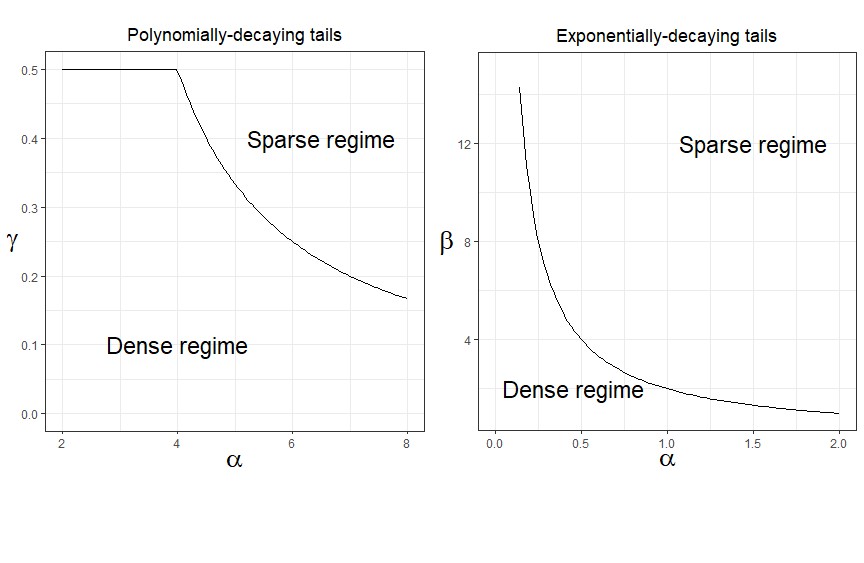
Figure 1: Minimax testing rate transition boundaries between dense and sparse regimes when the distribution of the error matrix belongs to $\mathcal{P}_{\alpha,K}^{\otimes}$ (left panel) and $\mathcal{G}_{\alpha,K}^{\otimes}$ (right panel). The testing rates within each regime are detailed in Table 1. The left panel plots the curve $\gamma(\alpha)=(\alpha-2)^{-1}\wedge 1/2$ for $\alpha\in[2,\infty)$, and the two regimes are separated by $s^{*}_{\mathcal{P}}=p^{1/2-\gamma}$. The right panel plots the curve $\beta(\alpha)=2/\alpha$ for $\alpha\in(0,2]$, and the two regimes are separated by $s^{*}_{\mathcal{G}}=\sqrt{p}\log^{-\beta}(ep)$.

		Upper bound	Lower bound
$\mathcal{G}_{\alpha,K}^{\otimes}$	Dense	(i) $\sqrt{p\log\log(8n)}+\log\log(8n)$	(ii) $\sqrt{p(\log\log(8n))^{\omega_{1}}}+\log\log(8n)$
	Sparse	(iii) $s\log^{2/\alpha}(ep/s)+\log\log(8n)$	(iv) $s\log^{2/\alpha}(ep/s)+\log\log(8n)$
$\mathcal{P}_{\alpha,K}^{\otimes}$	Dense	(v) $p^{(2/\alpha)\vee(1/2)}\log\log(8n)$	(vi) $p^{(2/\alpha)\vee(1/2)}\sqrt{(\log\log(8n))^{\omega_{2}}}+\log\log(8n)$
	Sparse	(vii) $s(p/s)^{2/\alpha}+\log\log(8n)$	(viii) $s(p/s)^{2/\alpha}+\log\log(8n)$

Table 1: Minimax testing rates up to $\log\log(8n)$ for a single mean change, where $\omega_{1}=\mathbbm{1}{\bigl{\{}s>\sqrt{p\log\log(8n)}\bigr{\}}}$ and $\omega_{2}=\mathbbm{1}{\bigl{\{}s>\sqrt{p\log\log(8n)}\;\text{and}\;\alpha\geq 4\}}$. The rows of $\mathcal{G}_{\alpha,K}^{\otimes}$ and $\mathcal{P}_{\alpha,K}^{\otimes}$ correspond to the right and left panel of Figure 1, respectively.

1.2 Relation to existing literature

Many real world data such as financial returns and macroeconomic variables exhibit heavy-tail phenomena, which often violate the convenient sub-Gaussian/exponential assumptions adopted by data analysts. Statistical procedures that mitigate the effects of heavy-tailed and/or contaminated data, therefore, have been sought after in practice, see Resnick (2007) for more in-depth discussions. Recent years have witnessed a growing interest among statisticians in quantifying the cost, if there is any, of heavy-tailedness on various statistical tasks. Notably, for the seemingly simple task of mean estimation, a range of innovative and sophisticated robust estimators (e.g. Catoni, 2012; Devroye et al., 2016; Lugosi and Mendelson, 2019a, b; Prasad et al., 2019; Depersin, 2020; Depersin and Lecué, 2022) are developed to achieve the same high probability upper bounds as in the Gaussian case, even if the data distribution is only assumed to have finite second moment. These results show that, in terms of convergence rates, there is no fundamental cost of allowing for heavy-tailed distributions for the task of mean estimation. With the success of mean estimation, a variety of statistical tasks are considered in the literature with the goal of developing estimators with Gaussian-like performances for heavy-tailed data, including regression (e.g. Fan et al., 2014; Lugosi and Mendelson, 2019a; Sun et al., 2020), empirical risk minimisation (e.g. Lecué and Lerasle, 2020; Prasad et al., 2020), matrix estimation (e.g. Minsker, 2018; Mendelson and Zhivotovskiy, 2020), among others. However, literature regarding change point analysis under heavy-tailed errors has been scarce in general.

One line of recent works (e.g. Cho and Owens, 2022; Wang and Zhao, 2022; Xu et al., 2022) consider change point models with exponentially-decaying heavy-tailed noise and study the performance of non-robust algorithms that perform well under sub-Gaussian noise assumptions. Theoretical results therein all require stronger assumptions on the strength of change points compared to the setting under sub-Gaussian assumptions. One motivation for our work is thus to investigate to what extent ideas from robust statistics are useful in analysing change points within high-dimensional heavy-tailed data streams.

Another line of attack develops algorithms with robust components for change point analysis. In particular, in the univariate mean change setting, Fearnhead and Rigaill (2019) propose to swap the commonly used $\ell_{2}$-loss with other loss functions, including the biweight and Huber loss functions to enhance robustness against heavy-tailed errors in localising change points. Li and Yu (2021) deploy a robust mean estimator with a scanning window idea to estimate multiple change point locations under a more general Huber contamination framework. Their results show that, in terms of the minimax detection boundary, there is essentially no cost of relaxing the sub-Gaussian assumption to more flexible finite moment assumptions. Robust change point analysis methodologies have also been proposed in other contexts including change point detection in stump models (Mukherjee et al., 2022), high-dimensional linear models (Liu et al., 2022) and functional time series (Wegner and Wendler, 2022), as well as detecting covariance changes (Ramsay and Chenouri, 2020) and distributional changes (Chenouri et al., 2020). Another series of works focus on robust online change point detection (e.g. Unnikrishnan et al., 2011; Cao and Xie, 2017; Molloy and Ford, 2017), which is different from the offline version that we study here.

Closer to our high-dimensional mean change point setting, Yu and Chen (2022) and Jiang et al. (2023) both consider the testing problem (2) and propose robust methodology targeting at sparse and dense changes, respectively. Yu and Chen (2022) formulate the problem as testing location parameter change, which in contrast to our model, allows the noise distribution to have mean parameter being infinite. Their methodology involves a U-statistic with an anti-symmetric and bounded kernel, followed by an $\ell_{\infty}$ aggregation. The power analysis of their proposed test (cf. Theorem 3.3 therein) along with subsequent remarks provide finite sample results showing that their test is able to detect the change point when it is sufficiently away from the boundary. In particular, their Remark 4 suggests that detection is only possible for local alternative when the change point location satisfies

$$t_{0}\wedge(n-t_{0})\geq c\sqrt{n\log(np)},$$

for some absolute constant $c>0$. In comparison, our results hold for the parameter space $\Theta(p,n,s,\rho)$ that covers all possible locations of change point. Moreover, as discussed in Remark 5 therein, their procedure achieves the sparse regime rate in $v^{*}_{{N}^{\otimes}(0,1)}(p,n,s)$ up to a poly-logarithmic factor in $n$ and $p$ only when $t_{0}=cn$ for some fixed constant $c\in(0,1)$. Jiang et al. (2023) consider the same mean change point testing problem as ours but without sparsity constraints. They allow a form of weak spatial dependence across coordinates and we discuss this aspect in Section 5. In terms of methodology, they also utilise a robustified U-statistic and combine it with the self-normalisation technique. They derive the limiting distributions of the proposed test under the sequential asymptotics. It is discussed in Remark 2 therein that, asymptotically, their test achieves the dense rate $v^{*}_{{N}^{\otimes}(0,1)}(p,n,p)$ up to a logarithmic factor in $n$, when the change point location satisfies $t_{0}=cn$ for some fixed constant $c\in(0,1)$.

In comparison to the results in Yu and Chen (2022) and Jiang et al. (2023), our results, as summarised in Section 1.1, are non-asymptotic and reveal that when considering the whole parameter space $\Theta(p,n,s,\rho)$, where the change point locations may be arbitrarily close to the boundary, the fundamental difficulty of the testing problem changes drastically. In particular, the heavy-tailed distributions manifest a strong impact on the minimax testing rates and one can no longer achieve the Gaussian-like minimax testing rates, especially in the sparse regime. Moreover, our results are generally sharper in the sense that we character the minimax testing rates up to a factor of at most $\log\log(8n)$.

Lastly, we mention two recent works – Comminges et al. (2021) and Liu et al. (2021) – that are technically related to ours. Comminges et al. (2021) study the sparse sequence models where

$$Y_{i}=\theta_{i}+\sigma\xi_{i},\quad i=1,\dotsc,p.$$

The noise random variables $\xi_{i}$ are i.i.d. with some distribution belonging to either $\mathcal{G}_{\alpha,K}$ or $\mathcal{P}_{\alpha,K}$, and the signal $\theta$ is assumed to be $\ell_{0}$-sparse with sparsity $s$. They provide minimax rates for estimating $\|\theta\|_{2}$ among other results (cf. Table 1 therein) under these two noise classes. Our results recover theirs when $n$ is of constant order and provide a link between these two problems, while significantly generalising to the arbitrary $n$ case. To achieve the minimax estimation rates, Comminges et al. (2021) first estimate $\theta$ via a penalised least squares estimator $\hat{\theta}$ in the sparse regime, and use $\|\hat{\theta}\|_{2}$ as an estimator for $\|\theta\|_{2}$. We adopt a different yet more intuitive hard-thresholding methodology in extracting information from sparse changes. Moreover, their upper bound rate under $\mathcal{P}_{\alpha,K}$ requires the assumption of bounded fourth moments, i.e. $\alpha\geq 4$. We investigate the more challenging case when $\alpha\in[2,4)$ and unveil a previously unknown phase transition behaviour even when $n$ is of constant order.

Liu et al. (2021) study the same testing problem (2) as ours under the Gaussian noise assumption while also considering spatial and temporal dependence. Their proposed testing procedure computes CUSUM-type statistics (e.g. Page, 1955) at each location on a dyadic grid. This also serves as the starting point of various procedures in our work. By comparing the results in Table 1 with the rate $v^{*}_{{N}^{\otimes}(0,1)}(p,n,s)$ derived by Liu et al. (2021) under the Gaussianity assumption, we show that the heavy-tailed errors mainly affect the difficulty of testing sparse changes, whereas in the $\mathcal{P}_{\alpha,K}^{\otimes}$ case with $\alpha\in[2,4)$, the dense rate also changes dramatically. In the special case of $p=s=1$, our results (both upper and lower bounds in all cases) reduce to $\log\log(8n)$, which is the same rate as $v^{*}_{{N}^{\otimes}(0,1)}(1,n,1)$. This shows that, in the univariate setting, there is no extra cost of allowing for heavy-tailed errors in testing change point compared to Gaussian errors.

1.3 Outline

The rest of paper is organised as follows. In Section 2, we study the testing problem (2) under sub-Weibull noise distributions, i.e. when $P_{e}\in\mathcal{G}_{\alpha,K}^{\otimes}$. We consider separately the dense and sparse regimes in Sections 2.1 and 2.2. In particular, the rates (i) – (iv) of Table 1 are established in 1, 2, 3 and 4, respectively. In Section 3, we consider the testing problem under finite moment assumptions on the noise distribution, i.e. when $P_{e}\in\mathcal{P}_{\alpha,K}^{\otimes}$. We again consider separately the dense and sparse regimes in Sections 3.1 and 3.2. We prove the rates (v) – (viii) of Table 1 in 5, 6, 9 and 10, respectively. The upper bound rates in Tables 1, particularly those in the sparse regimes, are achieved by procedures that require the knowledge of the sparsity parameter. We propose and study procedures that are adaptive to the unknown sparsity level in Section 4. We conclude the paper with some discussions on potential future directions in Section 5. Proofs of our main results are given in Appendix A, with auxiliary results deferred to Appendix B.

1.4 Notation

We end this section by introducing some notation used throughout the paper. For $d\in\mathbb{N}^{*}$, we write $[d]:=\{1,\dotsc,d\}$. Given $a,b\in\mathbb{R}$, we denote $a\wedge b:=\min(a,b)$ and $a\vee b:=\max(a,b)$. For a set $S$, we use $\mathbbm{1}_{S}$ and $|S|$ to denote its indicator function and cardinality respectively. For a vector $v=\bigl{(}v(1),\dotsc,v(d)\bigr{)}^{\top}\in\mathbb{R}^{d}$, we define $\|v\|_{0}:=\sum_{i=1}^{d}\mathbbm{1}_{\{v(i)\neq 0\}}$, $\|v\|_{2}:=\bigl{\{}\sum_{i=1}^{d}v(i)^{2}\bigr{\}}^{1/2}$ and $\|v\|_{\infty}:=\max_{i\in[d]}|v(i)|$. For a matrix $A=(A_{ij})_{i\in[d_{1}],j\in[d_{2}]}=\bigl{(}A_{j}(i)\bigr{)}_{i\in[d_{1}],j\in[d_{2}]}\in\mathbb{R}^{d_{1}\times d_{2}}$, we denote the Frobenius norm $\|A\|_{\mathrm{F}}:=\bigl{\{}\sum_{i=1}^{d_{1}}\sum_{j=1}^{d_{2}}A_{ij}^{2}\bigr{\}}^{1/2}$, the operator norm $\|A\|_{2}:=\max_{v\in\mathbb{R}^{d_{2}},v\neq 0}\|Av\|_{2}/\|v\|_{2}$, the two-to-infinity norm $\|A\|_{2\rightarrow\infty}:=\max_{v\in\mathbb{R}^{d_{2}},v\neq 0}\|Av\|_{\infty}/\|v\|_{2}$ and the max norm $\|A\|_{\max}:=\max_{i\in[d_{1}],j\in[d_{2}]}|A_{ij}|$. We use $\Gamma(\cdot)$ to denote the gamma function. For two probability measures $P$ and $Q$ on a measurable space $(\mathcal{X},\mathcal{A})$, we denote the total variation distance between them as $\mathrm{TV}(P,Q):=\sup_{A\in\mathcal{A}}|P(A)-Q(A)|$. If, in addition, $P$ and $Q$ are absolute continuous with respect to some base measure $\lambda$, then we define the squared Hellinger distance between them as $\mathrm{H}^{2}(P,Q):=\int_{\mathcal{X}}\bigl{(}\sqrt{p(x)}-\sqrt{q(x)}\bigr{)}^{2}\,\lambda(dx)$, where $p$ and $q$ are the Radon–Nikodym derivatives of $P$ and $Q$ with respect to $\lambda$ respectively. Finally, when the distribution is clear from the context, we use $\mathbb{P}$, $\mathbb{E}$ and $\mathrm{Var}$ to denote probability, expectation and variance operators respectively.

2 Testing under sub-Weibull noise distribution

In this section, we consider the entries of the noise matrix $E$ to be independent random variables and each follows a distribution belonging to the class $\mathcal{G}_{\alpha,K}$, see 2. For any measurable test function $\phi:\mathbb{R}^{p\times n}\rightarrow\{0,1\}$ and $\rho>0$, we write the worst case testing error when $P_{e}\in\mathcal{G}_{\alpha,K}^{\otimes}$ as

$$\mathcal{R}_{\mathcal{G}}(\rho,\phi)=\sup_{P_{e}\in\mathcal{G}_{\alpha,K}^{\otimes}}\sup_{\theta\in\Theta_{0}(p,n)}\mathbb{E}_{\theta,P_{e}}(\phi)+\sup_{P_{e}\in\mathcal{G}_{\alpha,K}^{\otimes}}\sup_{\theta\in\Theta(p,n,s,\rho)}\mathbb{E}_{\theta,P_{e}}(1-\phi).$$

In some slight abuse of notation, we use $\mathcal{R}_{\mathcal{G}}$ (resp. $\mathcal{R}_{\mathcal{P}}$) in place of $\mathcal{R}_{\mathcal{G}_{\alpha,K}^{\otimes}}$ (resp. $\mathcal{R}_{\mathcal{P}_{\alpha,K}^{\otimes}}$) in the rest of this paper. Recall the minimax testing error, defined in 1, as

$$\mathcal{R}_{\mathcal{G}}(\rho)=\inf_{\phi\in\Phi}\mathcal{R}_{\mathcal{G}}(\rho,\phi).$$

We assume the sparsity level $s$ to be known for now and defer the discussion of adaptive procedures to Section 4. Given $s$, we separately consider the dense and sparse regimes as mentioned in Section 1.1. Recall that the boundary between these two regimes is

$$s^{*}_{\mathcal{G}}=\frac{\sqrt{p}}{\log^{2/\alpha}(ep)}.$$ (6)

The dense regime refers to the case $s\geq s^{*}_{\mathcal{G}}$, while the sparse regime refers to the case $s<s^{*}_{\mathcal{G}}$. The choice of this boundary is discussed at the end of this section.

2.1 Dense regime

In the dense regime, we consider the testing procedure that is used in Liu et al. (2021). Consider $\mathcal{T}=\bigl{\{}1,2,4,\dotsc,2^{\lfloor\log_{2}(n/2)\rfloor}\bigr{\}}$ and a CUSUM-type statistic

$$Y_{t}:=\frac{\sum_{i=1}^{t}X_{i}-\sum_{i=1}^{t}X_{n+1-i}}{\sqrt{2t}}.$$

We define our test as

$$\phi_{\mathcal{G},\mathrm{dense}}:=\mathbbm{1}_{\{\max_{t\in\mathcal{T}}A_{t}>r\}},$$ (7)

where

$$A_{t}:=\sum_{j=1}^{p}\bigl{\{}Y_{t}^{2}(j)-1\bigr{\}}$$ (8)

and $r>0$ is the detection threshold specified in (9) below. Note that it suffices to test for change point over the dyadic grid $\mathcal{T}$ since for any true change point location $t_{0}\in[n-1]$ under the alternative, there exists some $t\in\mathcal{T}$ such that $t\leq t_{0}\leq 2t$, which is at the optimal scale for testing the alternative parameter space $\Theta^{(t_{0})}(p,n,s,\rho)$. The logarithmic size of $\mathcal{T}$ is the main reason behind the appearance of the $\log\log(8n)$ terms in our bounds below. The following theorem establishes the theoretical guarantee of the test $\phi_{\mathcal{G},\mathrm{dense}}$.

Theorem 1.

Let $0<\alpha\leq 2$ and $K>0$. For any $\varepsilon\in(0,1)$, there exist constants $C_{1},C_{2}>0$ depending only on $\alpha$, $K$ and $\varepsilon$, such that the test $\phi_{\mathcal{G},\mathrm{dense}}$ defined in (7) with

$$r =C_{1}\bigl{(}\sqrt{p\log\log(8n)}+\log\log(8n)\bigr{)}$$ (9)

satisfies

$$\mathcal{R}_{\mathcal{G}}(\rho,\phi_{\mathcal{G},\mathrm{dense}})\leq\varepsilon,$$

as long as $\rho^{2}\geq C_{2}v_{\mathcal{G},\mathrm{dense}}^{\mathrm{U}},$ where

$$v_{\mathcal{G},\mathrm{dense}}^{\mathrm{U}}:=\sqrt{p\log\log(8n)}+\log\log(8n).$$

Note that this simple test actually achieves the same rate in the dense regime as $v_{N^{\otimes}(0,1)}^{*}$ defined in (3), saving for a slightly different separation boundary (see Section 2.3), even though the noise distributions possess heavier tails than Gaussian distribution. One key ingredient in successfully showing that there is no cost of allowing sub-Weibull distributions in the dense regime, is a careful analysis of the type-I error using Lemma 18 instead of a crude union bound.

Note also that the above result in fact holds for any known sparsity level $s\in[p]$. Combined with the following proposition, we show that the test $\phi_{\mathcal{G},\mathrm{dense}}$ in (7) is indeed minimax rate-optimal in the dense regime when $s\geq\sqrt{p\log\log(8n)}$ and up to $\sqrt{\log\log(8n)}$ otherwise. We carefully discuss this gap in Section 2.3.

Proposition 2.

Let $0<\alpha\leq 2$, $K\geq K_{\alpha}$ and $s\geq\sqrt{p}\log^{-2/\alpha}(ep)\vee c$, for some absolute constant $c>0$ and some constant $K_{\alpha}>0$ depending only on $\alpha$. There exists some constant $c^{\prime}>0$ depending only on $\alpha$ and $K$, such that $\mathcal{R}_{\mathcal{G}}(\rho)\geq 1/2$ whenever $\rho^{2}\leq c^{\prime}v_{\mathcal{G},\mathrm{dense}}^{\mathrm{L}}$, where

$$v_{\mathcal{G},\mathrm{dense}}^{\mathrm{L}}:=\sqrt{p(\log\log(8n))^{\omega}}+\log\log(8n),$$

and $\omega=\mathbbm{1}_{\bigl{\{}s\geq\sqrt{p\log\log(8n)}\bigr{\}}}$.

In view of 1 and 2, we see that under $\mathcal{G}_{\alpha,K}$, the heaviness of the tail does not impact the minimax testing rate in the dense regime (up to a possible iterated logarithmic factor). However, the $\alpha$ parameter does influence the boundary between the sparse and the dense regime. Specifically, as $\alpha$ decreases (i.e. the tail becomes heavier), the dense regime becomes larger, as illustrated in the right panel of Figure 1.

2.2 Sparse regime

In the sparse regime, we consider a sampling-splitting testing procedure where, intuitively, we first use half of the data to identify coordinates that exhibit strong signals of change, and then use the other half to aggregate the selected ‘signal’ coordinates. Such a methodology is applicable for testing potential change locations $t\in\mathcal{T}\setminus\{1\}$ and we deal with testing the special case of $t=1$ separately.

To be specific, for $t\in\mathcal{T}\setminus\{1\}$, we define a sample-splitting version of (8) as

$$Y_{t,1}:=\frac{\sum_{i=1}^{t/2}X_{2i-1}-\sum_{i=1}^{t/2}X_{n+1-2i}}{\sqrt{t}},\qquad Y_{t,2}:=\frac{\sum_{i=1}^{t/2}X_{2i}-\sum_{i=1}^{t/2}X_{n+2-2i}}{\sqrt{t}},$$ (10)

and consider the following test

$$\phi_{\mathcal{G},\mathrm{sparse}}:=\mathbbm{1}_{\{\max_{t\in\mathcal{T}\setminus\{1\}}A_{t,a}>r\}}\vee\mathbbm{1}_{\{A_{1,a}>r_{1}\}},$$ (11)

where

$$A_{t,a}:=\begin{cases}\sum_{j=1}^{p}\bigl{\{}Y_{t,1}^{2}(j)-1\bigr{\}}\mathbbm{1}_{\{|Y_{t,2}(j)|\geq a\}},&t\geq 2,\\ \sum_{j=1}^{p}\bigl{\{}Y_{t}^{2}(j)-1\bigr{\}}\mathbbm{1}_{\{|Y_{t}(j)|\geq a\}},&t=1,\end{cases}$$ (12)

and $a,r,r_{1}$ are parameters specified in (13). The following theorem establishes the theoretical guarantee of the test $\phi_{\mathcal{G},\mathrm{sparse}}$.

Theorem 3.

Let $0<\alpha\leq 2$ and $K>0$. For any $\varepsilon\in(0,1)$, there exist constants $C_{1},C_{2},C_{3},C_{4}>0$ depending only on $\alpha$, $K$ and $\varepsilon$, such that the test $\phi_{\mathcal{G},\mathrm{dense}}$ defined in (11) with

$$a =C_{1}\bigl{(}\log^{1/\alpha}(ep/s)+s^{-1/2}\log^{1/2}(\log(8n))\bigr{)},$$ (13)

$$r =C_{2}\bigl{(}\sqrt{s\log\log(8n)}+\log\log(8n)\bigr{)},$$

$$r_{1} =C_{3}s\log^{2/\alpha}(ep/s),$$

satisfies

$$\mathcal{R}_{\mathcal{G}}(\rho,\phi_{\mathcal{G},\mathrm{sparse}})\leq\varepsilon,$$

as long as $\rho^{2}\geq C_{4}v_{\mathcal{G},\mathrm{sparse}}^{\mathrm{U}},$ where

$$v_{\mathcal{G},\mathrm{sparse}}^{\mathrm{U}}:=s\log^{2/\alpha}(ep/s)+\log\log(8n).$$

The idea of selecting coordinates via hard-thresholding has been widely used and in particular, in the change point context, e.g. considered by Liu et al. (2021) under the Gaussian noise assumption. However, their test does not require sample-splitting due to the tractability of truncated non-central chi-square distribution. Such property disappears even when moving from Gaussian noise assumption to sub-Gaussian noise assumption and results in different rates in the sparse regime (see Section 7.1 in Pilliat et al., 2023). From a technical point of view, our use of sample-splitting prompts the independence between the coordinate selection and $\ell_{2}$ aggregation, simplifying the analysis while achieving the optimal testing rate. A test based on (12) but without using sample splitting can be shown to have a slightly worse testing rate of $s\log^{2/\alpha}(ep/s)+\log(es)\log\log(8n)$ with our current proof technique.

Proposition 4.

Let $0<\alpha\leq 2$, $K\geq K_{\alpha}$ and $c\leq s\leq\sqrt{p}\log^{-2/\alpha}(ep)$, for some absolute constant $c>0$ and some constant $K_{\alpha}>0$ depending only on $\alpha$. There exists some constant $c^{\prime}>0$ depending only on $\alpha$ and $K$, such that $\mathcal{R}_{\mathcal{G}}(\rho)\geq 1/2$ whenever $\rho^{2}\leq c^{\prime}v_{\mathcal{G},\mathrm{sparse}}^{\mathrm{L}}$, where

$$v_{\mathcal{G},\mathrm{sparse}}^{\mathrm{L}}:=s\log^{2/\alpha}(ep/s)+\log\log(8n).$$

The above proposition, combined with 3, shows that the test $\phi_{\mathcal{G},\mathrm{sparse}}$ achieves the minimax testing rate in the sparse regime as long as the sparsity level is larger than an absolute constant, which arises as an artefact of our proof.

2.3 Discussion on the minimaxity gap

We conclude this section with some discussion on the gap between the upper bound rates $v_{\mathcal{G},\mathrm{dense}}^{\mathrm{U}}$, $v_{\mathcal{G},\mathrm{sparse}}^{\mathrm{U}}$ and the lower bound rates $v_{\mathcal{G},\mathrm{dense}}^{\mathrm{L}}$, $v_{\mathcal{G},\mathrm{sparse}}^{\mathrm{L}}$. Recall that each rate is a function of $p$, $n$ and $s$. A key observation is that Theorems 1 and 3 hold for any sparsity level $s$. In other words, for any given $s$, we can simultaneously run the two testing procedures described in Sections 2.1 and 2.2 and take $\phi_{\mathcal{G},\mathrm{dense}}\vee\phi_{\mathcal{G},\mathrm{sparse}}$ as our test. This leads to an upper bound

$$v_{\mathcal{G},\mathrm{dense}}^{\mathrm{U}}(p,n,s)\wedge v_{\mathcal{G},\mathrm{sparse}}^{\mathrm{U}}(p,n,s)$$ (14)

on the minimax testing rate.

The separation boundary between dense and sparse regimes based on (14) is $s_{\mathcal{G}}$ which satisfies $v_{\mathcal{G},\mathrm{dense}}^{\mathrm{U}}(p,n,s_{\mathcal{G}})=v_{\mathcal{G},\mathrm{sparse}}^{\mathrm{U}}(p,n,s_{\mathcal{G}})$, i.e. $\sqrt{p\log\log(8n)}=s_{\mathcal{G}}\log^{2/\alpha}(ep/s_{\mathcal{G}})$. Define $\zeta_{\mathcal{G}}(s):=s\log^{2/\alpha}(e^{2/\alpha}p/s)$, which is increasing in $s$ when $1\leq s\leq p$. Then $s_{\mathcal{G}}$ is of the same order as $\zeta_{\mathcal{G}}^{-1}(\sqrt{p\log\log(8n)})$. This is a slightly different boundary from $s^{*}_{\mathcal{G}}=\sqrt{p}\log^{-2/\alpha}(ep)$ that we defined in (6), which is of the same order as $\zeta_{\mathcal{G}}^{-1}(\sqrt{p})$. Note that $s^{*}_{\mathcal{G}}$ does not depend on the sample size $n$ while $s_{\mathcal{G}}$ does. Observe also that due to the monotonicity of $s\mapsto\zeta_{\mathcal{G}}(s)$ , we have $s^{*}_{\mathcal{G}}\leq C_{\alpha}s_{\mathcal{G}}<\sqrt{p\log\log(8n)}$ for some constant $C_{\alpha}>0$ depending only on $\alpha$.

In our sparse regime $s<s^{*}_{\mathcal{G}}$, the rate in (14) simply becomes $v_{\mathcal{G},\mathrm{sparse}}^{\mathrm{U}}(p,n,s)$, and exactly matches the lower bound $v_{\mathcal{G},\mathrm{sparse}}^{\mathrm{L}}(p,n,s)$. In our dense regime, we first focus on the regime $s\geq\sqrt{p\log\log(8n)}$. The rate in (14) is now $v_{\mathcal{G},\mathrm{dense}}^{\mathrm{U}}(p,n,s)$ and again matches the corresponding lower bound $v_{\mathcal{G},\mathrm{dense}}^{\mathrm{L}}(p,n,s)$. We remark that $s\geq\sqrt{p\log\log(8n)}$ is in fact the ‘dense regime’ under Gaussian noise assumption (Liu et al., 2021, Theorem 1).

The more intriguing region of the sparsity level is $s^{*}_{\mathcal{G}}\leq s<\sqrt{p\log\log(8n)}$, where we have used the dense version of the test in Section 3.1 to achieve a rate of $v_{\mathcal{G},\mathrm{dense}}^{\mathrm{U}}(p,n,s)$. Note that a gap of $\sqrt{\log\log(8n)}$ exists between $v_{\mathcal{G},\mathrm{dense}}^{\mathrm{U}}(p,n,s_{\mathcal{G}})$ and $v_{\mathcal{G},\mathrm{dense}}^{\mathrm{L}}(p,n,s_{\mathcal{G}})$. When $s^{*}_{\mathcal{G}}\leq s\leq s_{\mathcal{G}}$, we can use the sparse version of test described in Section 2.2 to achieve the rate in (14), which provides a small improvement over $v_{\mathcal{G},\mathrm{dense}}^{\mathrm{U}}(p,n,s)$. In fact, any sparsity level between $s^{*}_{\mathcal{G}}$ and $\sqrt{p\log\log(8n)}$ can be chosen to be the boundary between using the dense test (7) and using the sparse test (11) and leads to an overall minimaxity gap of order $\sqrt{\log\log(8n)}$. For ease of exposition, we have used $s^{*}_{\mathcal{G}}$ as this boundary, as it has a simple closed form expression depending only on $p$.

Lastly, we note that the gap discussed in the last paragraph even exists when each entry of the noise matrix follows a sub-Gaussian distribution rather than a standard normal; see Pilliat et al. (2023, Section 7.1), where it is suggested that a procedure that explores the exact distribution of the noise may be able to further close this gap.

3 Testing under finite moment noise distribution

In this section, we consider the case when $P_{e}\in\mathcal{P}_{\alpha,K}^{\otimes}$, or equivalently, we assume that the distribution of each entry in the noise matrix $E$ has only finitely $\alpha$-th moments, for some constant $\alpha\geq 2$, see 3. Compared to the $\mathcal{G}_{\alpha,K}$ class of distributions that we considered in Section 2, the $\mathcal{P}_{\alpha,K}$ class of distributions include a much wider range of noise distributions, e.g. $t$ distributions and centred Pareto distributions. As a result, it poses a much large statistical challenge, and new approaches to tackle the testing problem are required.

The results developed in Section 2 show that, when the noise distributions belong to the sub-Weibull class, standard CUSUM-type testing procedure can already achieve near-optimal minimax testing rate (up to $\sqrt{\log\log(8n)}$). Using more advanced tools from robust statistics is unlikely to result in major improvement on the testing rate. However, when the error distribution has a much heavier tail, i.e. only decays polynomially, which implies the existence of only finitely many moments, the story is different. Using CUSUM-type statistics alone will not be enough to obtain ideal performance due to a lack of sharp concentration in such settings. We therefore borrow wisdom from robust statistics in pursuit of better concentration around true change point signals.

Similar to the sub-Weibull case, we write the worst case testing error as $\mathcal{R}_{\mathcal{P}}(\rho,\phi)$ and the minimax testing error as $\mathcal{R}_{\mathcal{P}}(\rho)$. Also, we assume the sparsity level to be known and consider the dense and sparse cases separately as in Sections 1.1 and 2. The boundary between these two regimes is now

$$s^{*}_{\mathcal{P}}:=p^{\frac{1}{2}-(\frac{1}{\alpha-2}\wedge\frac{1}{2})},$$ (15)

and the dense regime refers to the case $s\geq s^{*}_{\mathcal{P}}$, while the sparse regime refers to its complement. The discussion on the boundary are left to Section 3.3. Notably, when $\alpha\in[2,4]$, we always have

$$\frac{1}{\alpha-2}\wedge\frac{1}{2}=\frac{1}{2},$$

which shows that there is no sparse regime in this extremely heavy-tailed setting.

3.1 Dense regime

We now describe our testing procedure for dense changes, building on the idea of median-of-means in robust statistics literature. For $i\leq n/2$, we denote $Z_{i}:=(X_{i}-X_{n-i+1})/\sqrt{2}$. For $t\in\mathcal{T}$, we split $\{Z_{1},\dotsc,Z_{t}\}$ into $G_{t}$ groups of equal size that

$$\mathcal{Z}_{t,1},\mathcal{Z}_{t,2},\dotsc,\mathcal{Z}_{t,G_{t}},$$

where each group contains $t/G_{t}\geq 1$ elements and the number of groups $G_{t}$ is specified later in (18). Note that our choice of $G_{t}$ will guarantee that $t/G_{t}$ is a positive integer. Set $V_{t,g}\in\mathbb{R}^{p}$ with

$$V_{t,g}(j):=\overline{Z}^{2}_{t,g}(j)-\frac{G_{t}}{t},$$

where $\overline{Z}_{t,g}\in\mathbb{R}^{p}$ is the sample mean of the $g$-th group. This quantity $V_{t,g}$ can be thought as a scaled version of the statistic $A_{t}$, defined in (8), but computed using only a subset of the data. To achieve robustness against heavy-tailed errors, we consider the following median-of-means type statistic

$$A_{t}^{\mathrm{MoM}}:=t\cdot\mathrm{median}\Biggl{(}\sum_{j=1}^{p}V_{t,1}(j),\sum_{j=1}^{p}V_{t,2}(j),\dotsc,\sum_{j=1}^{p}V_{t,G_{t}}(j)\Biggl{)}.$$ (16)

Our test is denoted as

$$\phi_{\mathcal{P},\mathrm{dense}}:=\mathbbm{1}_{\left\{\max_{t\in\mathcal{T}}A_{t}^{\mathrm{MoM}}/r_{t}>1\right\}},$$ (17)

with the detection threshold $r_{t}$ to be specified in (18). Before presenting the theoretical guarantee of the test $\phi_{\mathcal{P},\mathrm{dense}}$ in 5, we first briefly explain the significance of median-of-means type statistics and the novelty of our procedure.

Median-of-means type statistics like (16) have been widely applied in the context of mean estimation (Lugosi and Mendelson, 2019b), empirical risk minimisation (Lerasle and Oliveira, 2011; Lecué and Lerasle, 2020) with applications to regression and density estimation problems (Humbert et al., 2022), estimator selection (Kwon et al., 2021) and classification (Lecué and Lerasle, 2020), among others. Arguably, the most well-known and simplest form is the median-of-means estimator for univariate mean estimation. Suppose that we have i.i.d. data of size $n$ with mean $\mu$ and variance $\sigma^{2}$. The median-of-means estimator $\hat{\mu}^{\mathrm{MoM}}$ is obtained by first partitioning the data into $G$ groups of equal size, then calculating the sample mean within each group and finally computing the median of these $G$ samples means. It is shown in Lugosi and Mendelson (2019a, Theorem 2) that, for $\delta\in(0,1)$, when the number of groups $G$ is chosen to be at least $8\log(1/\delta)$, then with probability at least $1-\delta$, the estimator $\hat{\mu}^{\mathrm{MoM}}=\hat{\mu}^{\mathrm{MoM}}(\delta)$ satisfies

$$|\hat{\mu}^{\mathrm{MoM}}-\mu|\leq\sigma\sqrt{\frac{32\log(1/\delta)}{n}}.$$

Thus, the median-of-means estimator can achieve sub-Gaussian performance in mean estimation under only the assumption of finite second moment.

However, in our context, the aforementioned methodology is not applicable for testing potential change point that is close to the boundary, as we will not have enough data to ensure good statistical guarantees. Therefore, for $t\in\mathcal{T}$ such that $t\leq\Delta$ with the threshold $\Delta$ specified later in (18), we essentially directly take the median of $t$ statistics in (16), i.e. $G_{t}=t$. Another challenge in our context lies in analysing the performance of our test when $\alpha\in[2,4]$. Since we compute a second order statistic $V_{t,g}$ within each group $g$, standard analysis would require a bounded fourth moment condition on the distribution. We are able to extend our result to this more challenging case of $\alpha\in[2,4]$, which is critical in unveiling a new phase transition phenomenon that is previously unknown even when $n$ is of constant order.

Theorem 5.

Assume $\alpha\geq 2$. For any $\varepsilon\in(0,1)$, there exist $C_{1},C_{2}>0$ depending only on $\alpha$, $K$ and $\varepsilon$, such that the test $\phi_{\mathcal{P},\mathrm{dense}}$ defined in (17) with

$$r_{t}=C_{1}p^{(1/2)\vee(2/\alpha)}G_{t},\quad G_{t}=t\wedge\Delta\quad\mbox{and}\quad\Delta=2^{3+\lceil\log_{2}\log\log(8n)\rceil},$$ (18)

satisfies that

$$\mathcal{R}_{\mathcal{P}}(\rho,\phi_{\mathcal{P},\mathrm{dense}})\leq\varepsilon,$$

as long as $\rho^{2}\geq C_{2}v_{\mathcal{P},\mathrm{dense}}^{\mathrm{U}}$, where

$$v_{\mathcal{P},\mathrm{dense}}^{\mathrm{U}}:=p^{(2/\alpha)\vee(1/2)}\log\log(8n)$$

The following proposition shows that the test $\phi_{\mathcal{P},\mathrm{dense}}$ is minimax rate-optimal up to $\log\log(8n)$ in the dense regime. More specifically, the gap is of order $\sqrt{\log\log(8n)}$ when $s>\sqrt{p\log\log(8n)}$ and $\alpha\geq 4$ and of order $\log\log(8n)$ otherwise. We carefully discuss this gap in Section 3.3.

Proposition 6.

Let $\alpha\geq 2$, $K\geq K_{\alpha}$ and $s\geq p^{\frac{1}{2}-(\frac{1}{\alpha-2}\wedge\frac{1}{2})}\vee c$, for some absolute constant $c>0$ and some constant $K_{\alpha}>0$ depending only on $\alpha$. There exists some constant $c^{\prime}>0$ depending only on $\alpha$ and $K$, such that $\mathcal{R}_{\mathcal{P}}(\rho)\geq 1/2$ whenever $\rho^{2}\leq c^{\prime}v_{\mathcal{P},\mathrm{dense}}^{\mathrm{L}}$, where

$$v_{\mathcal{P},\mathrm{dense}}^{\mathrm{L}}:=p^{(2/\alpha)\vee(1/2)}(\log\log(8n))^{\omega/2}+\log\log(8n)$$

with $\omega=\mathbbm{1}_{\bigl{\{}s>\sqrt{p\log\log(8n)}\bigr{\}}\cap\{\alpha\geq 4\}}$.

Compared to the remark following 2, we see that for $\alpha\geq 4$, the parameter $\alpha$, which encodes the heaviness of the tails, again only affects the boundary between the dense and the sparse regimes, as illustrated in the left panel of Figure 1, and does not change the minimax testing rate in the dense regime itself. On the other hand, when $\alpha\in[2,4]$, the boundary no longer varies with $\alpha$, but the minimax testing rate in the dense regime increases as $\alpha$ decreases.

A closer look at the condition $s\geq p^{\frac{1}{2}-(\frac{1}{\alpha-2}\wedge\frac{1}{2})}\vee c$ reveals that when $\alpha\in[2,4]$, the lower bound in 6 holds for essentially all sparsity levels except when $s$ is less than an absolute constant, which arises as an artefact of our proof. This means that the testing rates in this extreme heavy-tailed setting are, in fact, independent of $s$, which implies that it is impossible to exploit the sparse structure of the change in pursuit of better results. Therefore, in the subsequent discussion of sparse regime, we only consider the case of $\alpha\geq 4$.

3.2 Sparse regime

In the sparse regime, we take two steps towards constructing a computationally-efficient and minimax rate-optimal test denoted as $\phi_{\mathcal{P},\mathrm{sparse}}$, which is presented at the end of this section. This test achieves the testing rate

$$v_{\mathcal{P},\mathrm{sparse}}^{\mathrm{U}}:=s(p/s)^{2/\alpha}+\log\log(8n),$$

as shown in 9 and it is the minimax optimal testing rate in the sparse regime as confirmed in 10.

A median-of-means-type test. Our first attempt is, at a high level, combining the median-of-means methodology developed in the dense regime Section 3.1 with the hard-thresholding coordinate selection technique used in Section 2.2. Recall that $Z_{i}=(X_{i}-X_{n-i+1})/\sqrt{2}$, for $i\leq n/2$. For $t\in\mathcal{T}\backslash\{1\}$, we split $\{Z_{1},\dotsc,Z_{t}\}$ into two halves: $\{Z_{1},Z_{3},\dotsc,Z_{t-1}\}$ and $\{Z_{2},Z_{4},\dotsc,Z_{t}\}$. We further split the first set into $G_{t}$ groups of equal size, denoted as

$$\mathcal{Z}_{t,1,1},\mathcal{Z}_{t,2,1},\dotsc,\mathcal{Z}_{t,G_{t},1},$$

with the number of groups $G_{t}$ specified later in (20), and use $\overline{Z}_{t,g,1}$ to denote the sample mean of the $g$-th group. Again, our choice of $G_{t}$ will guarantee $t/(2G_{t})$ to be a positive integer. The second set of samples $\{Z_{2},Z_{4},\dotsc,Z_{t}\}$ is reserved for selecting the signal coordinates as we did in Section 2.2. Consider the statistic $V_{t,g,a}\in\mathbb{R}^{p}$ with

$$V_{t,g,a}(j):=\biggl{(}\overline{Z}^{2}_{t,g,1}(j)-\frac{2G_{t}}{t}\biggr{)}\mathbbm{1}_{\{|Y_{t,2}(j)|\geq a\}},\quad j\in[p],$$

where $Y_{t,2}(j)$ is defined in (10) and $a$ is a selection threshold to be specified in (20). Our test statistic takes almost the same form as in the dense case

$$A_{t,a}^{\mathrm{MoM}}:=\frac{t}{2}\cdot\mathrm{median}\Biggl{(}\sum_{j=1}^{p}V_{t,1,a}(j),\sum_{j=1}^{p}V_{t,2,a}(j),\dotsc,\sum_{j=1}^{p}V_{t,G_{t},a}(j)\Biggl{)}.$$

For the case of $t=1$, we cannot perform sample-splitting and therefore we deal with it separately by considering

$$A_{1,a}^{\mathrm{MoM}}:=A_{1,a}=\sum_{j=1}^{p}(Z_{1}^{2}(j)-1)\mathbbm{1}_{\{|Z_{1}(j)|\geq a\}}.$$

Finally, our test is

$$\phi_{\mathcal{P},\mathrm{sparse}}^{\mathrm{MoM}}:=\mathbbm{1}_{\{\max_{t\in\mathcal{T}}A_{t,a}^{\mathrm{MoM}}/r_{t}>1\}}.$$ (19)

The theoretical guarantee of $\phi_{\mathcal{P},\mathrm{sparse}}^{\mathrm{MoM}}$ is established in 7 below. It is worth mentioning that in the hard-thresholding step, we simply use the non-robust quantity $Y_{t,2}$ to estimate the signal of each coordinate instead of its robust counterparts. This is mainly to avoid further complication of the procedure since if, for example, the median-of-means estimator were deployed for each coordinate, then we would need to further split the data into groups and deal with the case when $t$ is close to the boundary.

Proposition 7.

Assume $\alpha\geq 4$. For any $\varepsilon\in(0,1)$, there exist $C_{1},C_{2},C_{3}>0$ depending only on $\alpha$, $K$ and $\varepsilon$, such that the test $\phi_{\mathcal{P},\mathrm{sparse}}^{\mathrm{MoM}}$ defined in (19) with

$$a=C_{1}\bigl{(}(p/s)^{1/\alpha}+s^{-1/2}\log^{1/2}(\log(8n))\bigr{)}, \quad r_{t}=C_{2}\bigl{(}s(p/s)^{2/\alpha}\mathbbm{1}_{\{t=1\}}+\sqrt{s}G_{t}\mathbbm{1}_{\{t>1\}}\bigr{)},$$ (20)

$$G_{t}=(t\wedge\Delta)/2 \mbox{and}\quad\Delta=2^{4+\lceil\log_{2}\log\log(8n)\rceil},$$

satisfies that

$$\mathcal{R}_{\mathcal{P}}(\rho,\phi_{\mathcal{P},\mathrm{sparse}}^{\mathrm{MoM}})\leq\varepsilon,$$

as long as $\rho^{2}\geq C_{3}v_{\mathcal{P},\mathrm{sparse}}^{\mathrm{U,MoM}}$, where

$$v_{\mathcal{P},\mathrm{sparse}}^{\mathrm{U,MoM}}:=s\bigl{(}(p/s)^{2/\alpha}+\log\log(8n)\bigr{)}.$$

A robust-sparse-mean-based test. The rate achieved by $\phi_{\mathcal{P},\mathrm{sparse}}^{\mathrm{MoM}}$ is slightly worse than the presented rate (vii) in Table 1. Our second attempt, in order to close this gap, is to use some robust sparse mean estimator in the literature to directly construct a test. One example of such estimator is given in Prasad et al. (2019):

$$\hat{\mu}^{\mathrm{RSM}}_{n,s}(\{W_{i}\}_{i=1}^{n};\eta):=\inf_{\mu\in\mathcal{L}_{s}}\sup_{u\in\mathcal{N}^{1/2}_{2s}(\mathcal{S}^{p-1})}|u^{\top}\mu-\mathrm{1DRobust}(\{u^{\top}W_{i}\}_{i=1}^{n},\eta/(6ep/s)^{s})|,$$ (21)

where $W_{1},\dotsc,W_{n}\in\mathbb{R}^{p}$ are input data, $\mathcal{L}_{s}:=\{v\in\mathbb{R}^{p}:\|v\|_{0}\leq s\}$ is the set of $s$-sparse vectors in $\mathbb{R}^{p}$, $\mathcal{N}^{1/2}_{2s}(\mathcal{S}^{p-1})$ is a $(1/2)$-cover of the set of $2s$-sparse unit vectors with cardinality $|\mathcal{N}^{1/2}_{2s}(\mathcal{S}^{p-1})|\leq(6ep/s)^{s}$ (Vershynin, 2009), and $\mathrm{1DRobust}$ is a univariate robust mean estimator defined in Prasad et al. (2019, Algorithm 2) based on the shorth estimator (e.g. Andrews and Hampel, 2015). One may naturally consider other univariate robust mean estimators in place of $\mathrm{1DRobust}$, including the median-of-means, as discussed briefly in Section 3.1 or trimmed mean variants (Lugosi and Mendelson, 2021). We note that (21) achieves a near-optimal statistical guarantee for the task of sparse mean estimation (Prasad et al., 2019, Corollary 11), despite its high computational complexity, scaling exponentially in $p$.

To this end, we describe the testing procedure using $\hat{\mu}^{\mathrm{RSM}}_{n,s}(\{W_{i}\}_{i=1}^{n};\eta)$ as an alternative of $\phi_{\mathcal{P},\mathrm{sparse}}^{\mathrm{MoM}}$. For $t\leq\tilde{\Delta}_{1}$, use the non-robust statistic $A_{t,a}$ as defined in (12). For $t\in\mathcal{T}\cap\{t>\tilde{\Delta}_{1}\}$, construct the statistic from the $\ell_{2}$ norm of this robust sparse mean estimator:

$$A^{\mathrm{RSM}}_{t}:=t\bigl{\|}\hat{\mu}_{t,s,\eta_{t}}^{\mathrm{RSM}}\bigr{\|}_{2}^{2}=t\bigl{\|}\hat{\mu}_{t,s}^{\mathrm{RSM}}(\{Z_{i}\}_{i=1}^{t};\eta_{t})\bigr{\|}_{2}^{2}.$$

With all the parameters $a,\tilde{\Delta}_{1},\tilde{\Delta}_{2},\tilde{r}_{t},r^{\mathrm{RSM}}_{t}$ and $\eta_{t}$ specified later in (23), our test is given by

$$\phi^{\mathrm{RSM}}_{\mathcal{P},\mathrm{sparse}}:=\mathbbm{1}_{\left\{\max_{t\in\mathcal{T}\cap\{t\leq\tilde{\Delta}_{1}\}}A_{t,a}/\tilde{r}_{t}>1\right\}}\vee\mathbbm{1}_{\left\{\max_{t\in\mathcal{T}\cap\{t>\tilde{\Delta}_{1}\}}A^{\mathrm{RSM}}_{t}/r^{\mathrm{RSM}}_{t}>1\right\}}.$$ (22)

The theoretical guarantee of $\phi^{\mathrm{RSM}}_{\mathcal{P},\mathrm{sparse}}$ is established in the following result.

Proposition 8.

Assume $\alpha\geq 4$. For any $\varepsilon\in(0,1)$, there exist $C_{1},C_{2},C_{3},C_{4},C_{5}>0$ depending only on $\alpha$, $K$ and $\varepsilon$, such that the test $\phi^{\mathrm{RSM}}_{\mathcal{P},\mathrm{sparse}}$ defined in (22) with

$$a=C_{1}\bigl{(}(p/s)^{1/\alpha}+s^{-1/2}\log^{1/2}(\log\tilde{\Delta}_{1})\bigr{)}, \quad\tilde{r}_{t}=C_{2}\Bigl{(}s(p/s)^{2/\alpha}\mathbbm{1}_{\{t=1\}}+\sqrt{s\log\tilde{\Delta}_{1}}\mathbbm{1}_{\{t>1\}}\Bigr{)},$$ (23)

$$\eta_{t}=\exp\biggl{\{}s\log(ep/s)-\frac{t\wedge\tilde{\Delta}_{2}}{C_{3}}\biggr{\}}, \quad r^{\mathrm{RSM}}_{t}=C_{4}(t\wedge\tilde{\Delta}_{2}),$$

$$\tilde{\Delta}_{1}=C_{3}\bigl{(}s\log(ep/s)+\log(16/\varepsilon)\bigr{)} \mbox{and}\quad\tilde{\Delta}_{2}=C_{3}\bigl{(}s\log(ep/s)+\log(16\log(2n)/\varepsilon)\bigr{)},$$

satisfies that

$$\mathcal{R}_{\mathcal{P}}(\rho,\phi^{\mathrm{RSM}}_{\mathcal{P},\mathrm{sparse}})\leq\varepsilon,$$

as long as $\rho^{2}\geq C_{5}v_{\mathcal{P},\mathrm{sparse}}^{\mathrm{U}}$, where

$$v_{\mathcal{P},\mathrm{sparse}}^{\mathrm{U}}=s(p/s)^{2/\alpha}+\log\log(8n).$$

Before addressing the issue of computation, several remarks are in order. The main reason we separate $t\in\mathcal{T}$ into different regions is, similar to the issue with median-of-means methods, that (21) cannot be applied when $t$ is too close to the boundary, and therefore, we need to resort to the non-robust testing statistics $A_{t,a}$. A more subtle issue which is critical in achieving, in fact, the optimal rate $v_{\mathcal{P},\mathrm{sparse}}^{\mathrm{U}}$, is that we apply the non-robust testing statistics only to a very small number of points in $\mathcal{T}$. Indeed, the boundary $\tilde{\Delta}_{1}$ is chosen to be independent of $n$ so that the power of (21) can be maximally exploited. Lastly, we mention that our proof of 8, which establishes the theoretical guarantee of $\phi^{\mathrm{RSM}}_{\mathcal{P},\mathrm{sparse}}$, is actually modular. Any other sparse mean estimator that satisfies a more general condition (1 in Section A.1.5) may be used in place of $\hat{\mu}_{t,s,\eta_{t}}^{\mathrm{RSM}}$ and the corresponding test achieves the same performance.

The combined test. As we mentioned before, one caveat of using a robust estimator such as (21), and in fact, a common issue in high-dimensional robust statistics in order to achieve good performance, is that the estimator is computationally-intractable since it often involves projecting the data onto every $2s$-sparse unit vectors or its covering set. As a result, even though the testing procedure $\phi^{\mathrm{RSM}}_{\mathcal{P},\mathrm{sparse}}$ in (22) performs better at detecting change point with weak signal compared to the previous median-of-means type test, the computational cost makes it not implementable in practice, especially when $p$ is large. The main result of this section, as presented in the theorem below, is a testing procedure that achieves the best of both worlds - computational efficiency and minimax optimality.

Theorem 9.

Assume $\alpha\geq 4$. Consider the test

$$\phi_{\mathcal{P},\mathrm{sparse}}:=\begin{cases}\phi_{\mathcal{P},\mathrm{sparse}}^{\mathrm{RSM}},&\text{if }p\leq\log^{\alpha-2}(\log(8n)),\\ \phi_{\mathcal{P},\mathrm{sparse}}^{\mathrm{MoM}},&\text{otherwise},\end{cases}$$

with the parameters of $\phi_{\mathcal{P},\mathrm{sparse}}^{\mathrm{MoM}}$ and $\phi_{\mathcal{P},\mathrm{sparse}}^{\mathrm{RSM}}$ chosen according to (20) and (23) respectively. It then holds that

$$\mathcal{R}_{\mathcal{P}}(\rho,\phi_{\mathcal{P},\mathrm{sparse}})\leq\varepsilon,$$

as long as $\rho^{2}\geq C_{1}v_{\mathcal{P},\mathrm{sparse}}^{\mathrm{U}}$, for some constant $C_{1}$, depending only on $\alpha$, $K$ and $\varepsilon$. Moreover, the computational complexity of $\phi_{\mathcal{P},\mathrm{sparse}}$ is polynomial in both $n$ and $p$.

9 is based on the following neat observation: by comparing $v_{\mathcal{P},\mathrm{sparse}}^{\mathrm{U},\mathrm{MoM}}$ and $v_{\mathcal{P},\mathrm{sparse}}^{\mathrm{U}}$, as established in 7 and 8 respectively, the improvement offered by $\phi^{\mathrm{RSM}}_{\mathcal{P},\mathrm{sparse}}$ over $\phi_{\mathcal{P},\mathrm{sparse}}^{\mathrm{MoM}}$ only exists when $p$ is sufficiently small. Therefore, we can bypass the computation barrier by using $\phi^{\mathrm{RSM}}_{\mathcal{P},\mathrm{sparse}}$ only when it outperforms $\phi_{\mathcal{P},\mathrm{sparse}}^{\mathrm{MoM}}$, which allows us to yield a combined testing procedure that has run time polynomial in $n$ and $p$ while achieving the optimal rate in the sparse regime.

Proposition 10.

Let $\alpha\geq 4$, $K\geq K_{\alpha}$ and $c\leq s\leq p^{\frac{1}{2}-\frac{1}{\alpha-2}}$, for some absolute constant $c>0$ and some constant $K_{\alpha}>0$ depending only on $\alpha$. There exists some constant $c^{\prime}>0$ depending only on $\alpha$ and $K$, such that $\mathcal{R}_{\mathcal{P}}(\rho)\geq 1/2$ whenever $\rho^{2}\leq c^{\prime}v_{\mathcal{P},\mathrm{sparse}}^{\mathrm{L}}$, where

$$v_{\mathcal{P},\mathrm{sparse}}^{\mathrm{L}}:=s(p/s)^{2/\alpha}+\log\log(8n).$$

Similar to the discussion following 4, we conclude from the above proposition and 9 that the combined test $\phi_{\mathcal{P},\mathrm{sparse}}$ achieves the minimax testing rate in the sparse regime as long as the sparsity level is larger than an absolute constant, which again arises as an artefact of our proof.

3.3 Discussion on the minimaxity gap

We start off with the case $\alpha\geq 4$, where there is a non-empty sparse regime $s<s^{*}_{\mathcal{P}}=p^{1/2-1/(\alpha-2)}$. Note that the boundary satisfies $s^{*}_{\mathcal{P}}=\zeta_{\mathcal{P}}^{-1}(\sqrt{p})$, where $\zeta_{\mathcal{P}}(s):=s(p/s)^{2/\alpha}$. Our first observation is that the upper and lower bounds on the minimax testing rate again match in the sparse regime. This is the same conclusion as in the sub-Weibull error setting. In the dense regime, note that for any sparsity level the upper and lower bounds on the minimax testing rates are only off by a factor of order at most $\log\log(8n)$. We explain this gap from two aspects. First, recall from the discussion in Section 2.3 that we have a minimaxity gap of $\sqrt{\log\log(8n)}$ in the dense regime under the sub-Weibull error distribution setting. This remains the case when we have polynomially-decaying tails.

We now explain the second component of the minimaxity gap. In the dense regime, we have $v_{\mathcal{P},\mathrm{dense}}^{\mathrm{U}}(p,n,s)=\sqrt{p}\log\log(8n)$. Comparing this with the dense regime upper bound rate in the sub-Weibull case $v_{\mathcal{G},\mathrm{dense}}^{\mathrm{U}}(p,n,s)=\sqrt{p\log\log(8n)}$, we observe an extra factor of $\sqrt{\log\log(8n)}$ when error distributions only have polynomially-decaying tails. We conjecture that our upper bound rate in the dense regime $v_{\mathcal{P},\mathrm{dense}}^{\mathrm{U}}(p,n,s)$ may not be tight, and propose a potential strategy to close this gap. Lugosi and Mendelson (2019b) among others show that, for $\delta\in(0,1)$, there exists a multivariate mean estimator $\hat{\mu}(\delta)$, such that for all distributions with mean $\mu$ and covariance $I_{p}$, with probability at least $1-\delta$,

$$\|\hat{\mu}(\delta)-\mu\|\leq C\biggl{(}\sqrt{\frac{p}{n}}+\sqrt{\frac{\log(1/\delta)}{n}}\biggr{)},$$ (24)

where $n$ is the sample size and $C$ is a universal constant. Consider an estimator $\hat{\mu}^{\prime}(\delta)$ that satisfies the following stronger condition similar to Laurent and Massart (2000, Lemma 1) for all distributions with finite fourth moment:

$$\|\hat{\mu}^{\prime}(\delta)-\mu\|^{2}_{2}-\frac{p}{n}\leq C\biggl{(}\frac{\sqrt{p\log(1/\delta)}}{n}+\frac{\log(1/\delta)}{n}\biggr{)}.$$ (25)

If we could find an estimator that satisfies (25), then it might help us improve the upper bound on the minimax testing rate from $\sqrt{p}\log\log(8n)$ to $\sqrt{p\log\log(8n)}$ in the dense regime, as Laurent and Massart (2000, Lemma 1) lies at the heart of proving the dense rate of $\sqrt{p\log\log(8n)}$ under Gaussian noise assumption in Liu et al. (2021). However, whether such a robust estimator exists remains an open question. Combining the two gaps discussed above, we conclude that for any sparsity level in the dense regime, the upper bound and the lower bound of the minimax testing rate are only off by a factor of order at most $\log\log(8n)$.

Lastly, we consider $2\leq\alpha<4$. We first note that for $\alpha=2$, the minimax optimal rate is $p+\log\log(8n)$. This can be shown by combining the lower bound derived from Section A.3 items (i) and (iii) and a test construction similar to (22) while replacing $\hat{\mu}^{\mathrm{RSM}}$ by a robust mean estimator $\hat{\mu}$ that satisfies (24). In view of the above minimax testing rates at $\alpha=2$ and $\alpha\geq 4$, we conjecture the precise minimax testing rates for $\alpha\in(2,4)$ to be

$$p^{2/\alpha}\log^{1-2/\alpha}\log(8n)+\log\log(8n).$$

Using Theorem 5 and Proposition 6, the best upper and lower bounds we can achieve in this regime are of the orders $p^{2/\alpha}\log\log(8n)$ and $p^{2/\alpha}+\log\log(8n)$ respectively. The precise exponent on $\log\log(8n)$ may have an interesting dependence on $\alpha$ that will need to be characterised in future research.

4 Adaptation to sparsity

In Sections 2 and 3, we have studied the change point testing problem under two types of heavy-tail assumptions on the error distributions: (1) exponentially-decaying/sub-Weibull tails and (2) finite $\alpha$-th moment assumption with $\alpha\geq 2$. The corresponding upper bound rates, e.g. $v_{\mathcal{G},\mathrm{sparse}}^{\mathrm{U}}$ and $v_{\mathcal{P},\mathrm{sparse}}^{\mathrm{U}}$, are currently achieved by testing procedures that take the sparsity level $s$ as an input. In other words, we have assumed the sparsity to be known up until now. In this section, we study the adaptation of these procedures to unknown sparsity levels.

First off, in the very heavy-tailed setting, i.e. each entry of $E$ has only finite $\alpha$-th moments for $\alpha\in[2,4]$, there is essentially no sparse regime, see the discussion following Proposition 6. The test $\phi_{\mathcal{P},\mathrm{dense}}$ defined in (17) with its parameters specified in Theorem 5 does not require the knowledge of the sparsity, and, therefore, the corresponding rate $v_{\mathcal{P},\mathrm{dense}}^{\mathrm{U}}=p^{2/\alpha}\log\log(8n)$ can already be achieved by an adaptive procedure.

We now focus on the case when $P_{e}\in\mathcal{P}_{\alpha,K}^{\otimes}$ for $\alpha>4$. Recall from Theorems 5 and 9 that $\phi_{\mathcal{P},\mathrm{dense}}$ and $\phi_{\mathcal{P},\mathrm{sparse}}$ achieve the rates $v_{\mathcal{P},\mathrm{dense}}^{\mathrm{U}}$ and $v_{\mathcal{P},\mathrm{sparse}}^{\mathrm{U}}$ respectively, when the sparsity is known. In the following, we introduce an adaptive testing procedure based on these two tests:

$$\phi_{\mathcal{P},\mathrm{adaptive}} :=\phi_{\mathcal{P},\mathrm{dense}}\vee\max_{s\in\mathcal{K}}{\phi}_{\mathcal{P},\mathrm{sparse},s}$$ (26)

$$\,=\begin{cases}\phi_{\mathcal{P},\mathrm{dense}}\vee\max_{s\in\mathcal{K}}{\phi}^{\mathrm{MoM}}_{\mathcal{P},\mathrm{sparse},s},&\text{if}\;p>\log^{\alpha-2}(\log(8n)),\\ \phi_{\mathcal{P},\mathrm{dense}}\vee\max_{s\in\mathcal{K}}{\phi}^{\mathrm{RSM}}_{\mathcal{P},\mathrm{sparse},s},&\text{if}\;p\leq\log^{\alpha-2}(\log(8n)),\end{cases}$$

where we make the dependence on $s$ explicit when referring to the sparse tests, and $\mathcal{K}:=\bigl{\{}1,2,4,\dotsc,2^{\lceil\log_{2}(p)\rceil-1}\bigr{\}}$ is a dyadic grid. Recall that $\phi_{\mathcal{P},\mathrm{dense}}$ does not require the knowledge of $s$, and we keep its original parameter choices as in (18), with perhaps an enlarged value of the leading constant $C_{1}$ in $r_{t}$:

$$r_{t}=C_{1}p^{(1/2)\vee(2/\alpha)}G_{t},\quad G_{t}=t\wedge\Delta\quad\mbox{and}\quad\Delta=2^{3+\lceil\log_{2}\log\log(8n)\rceil}.$$ (27)

For $\phi_{\mathcal{P},\mathrm{sparse},s}^{\mathrm{MoM}}$, we modify the original parameter choices (20) as follows:

$$a_{s}=C_{2}\bigl{(}(p/s)^{1/\alpha}+s^{-1/2}\log^{1/2}(\log(8n))\bigr{)}, \quad r_{t,s}=C_{3}\bigl{(}s(p/s)^{2/\alpha}\mathbbm{1}_{\{t=1\}}+s^{3/4}G_{t}\mathbbm{1}_{\{t>1\}}\bigr{)},$$ (28)

$$\quad G_{t}=(t\wedge\Delta)/2 \mbox{and}\quad\Delta=2^{4+\lceil\log_{2}\log\log(8n)\rceil}.$$

Compared with (20), we use the same $a_{s}$ (again with perhaps a larger leading constant) and modify $r_{t,s}$. Finally, for $\phi_{\mathcal{P},\mathrm{sparse},s}^{\mathrm{RSM}}$, we modify its original parameter choices (23) to be:

$$a_{s}=C_{4}\bigl{(}(p/s)^{1/\alpha}+s^{-1/2}\log^{1/2}(\log\tilde{\Delta}_{1,s})\bigr{)}, \quad\tilde{r}_{t,s}=C_{5}\Bigl{(}s(p/s)^{2/\alpha}\mathbbm{1}_{\{t=1\}}+s^{3/4}\sqrt{\log\tilde{\Delta}_{1}}\mathbbm{1}_{\{t>1\}}\Bigr{)},$$ (29)

$$\eta_{t,s}=\exp\biggl{\{}s\log(ep/s)-\frac{t\wedge\tilde{\Delta}_{2}}{C_{6}}\biggr{\}}, \quad r^{\mathrm{RSM}}_{t,s}=C_{7}(t\wedge\tilde{\Delta}_{2,s}),$$

$$\tilde{\Delta}_{1,s}=C_{6}\bigl{(}s\log(ep/s)+\log(80s/\varepsilon)\bigr{)} \mbox{and}\quad\tilde{\Delta}_{2,s}=C_{6}\bigl{(}s\log(ep/s)+\log(80s\log(2n)/\varepsilon)\bigr{)}.$$

Theorem 11.

Assume $\alpha\geq 4$. For any $\varepsilon\in(0,1)$, there exist $C_{1},\dotsc,C_{8}>0$ depending only on $\alpha$, $K$ and $\varepsilon$, such that the test $\phi_{\mathcal{P},\mathrm{adaptive}}$ defined in (26) with its parameters specified in (27), (28) and (29) satisfies

$$\mathcal{R}_{\mathcal{P}}(\rho,\phi_{\mathcal{P},\mathrm{adaptive}})\leq\varepsilon,$$

as long as $\rho^{2}\geq C_{8}\bigl{(}v_{\mathcal{P},\mathrm{dense}}^{\mathrm{U}}\wedge v_{\mathcal{P},\mathrm{sparse}}^{\mathrm{U}}\bigr{)}$.

11 establishes the theoretical guarantee of the adaptive test $\phi_{\mathcal{P},\mathrm{adaptive}}$ which does not require the knowledge of the sparsity parameter. Note that the rate that it achieves, i.e. $v_{\mathcal{P},\mathrm{dense}}^{\mathrm{U}}\wedge v_{\mathcal{P},\mathrm{sparse}}^{\mathrm{U}}$, matches the lower bound in the sparse regime $s<s^{*}_{\mathcal{P}}$, where $s^{*}_{\mathcal{P}}$ is defined in (15), while a gap of order up to $\log\log(8n)$ exists in the dense regime $s\geq s^{*}_{\mathcal{P}}$; see Section 3.3 for a thorough discussion on this gap. When the errors have exponentially-decaying tails instead, a similar adaptive testing procedure can be constructed based on $\phi_{\mathcal{G},\mathrm{dense}}$ and $\phi_{\mathcal{G},\mathrm{dense}}$ and achieve the rate $v_{\mathcal{G},\mathrm{dense}}^{\mathrm{U}}\wedge v_{\mathcal{G},\mathrm{sparse}}^{\mathrm{U}}$. For the sake of brevity, we omit further details here.

5 Discussion

In this paper, we have studied the problem of testing against a single mean change point for high-dimensional heavy-tailed data. We have characterised the minimax testing rates of this problem up to $\sqrt{\log\log(8n)}$ in the case of exponentially-decaying tails, and up to $\log\log(8n)$ in the case of polynomially-decaying tails. Thorough discussions on these gaps are provided in Sections 2.3 and 3.3. In addition, our results quantify the costs of heavy-tailed distributions in this problem by comparing to the previous results under Gaussian error assumption (Liu et al., 2021) and unveil a new phenomenon that the minimax testing rates of mean change point problem undergo a phase transition when the error distribution has finite fourth moment. It is known that for the mean estimation problem, the fundamental difficulty change drastically when the distribution has fewer than two finite moments (e.g. Bubeck et al., 2013; Cherapanamjeri et al., 2022). Our results suggest that detecting mean change is rather different from mean estimation and, in fact, has close links to the problem of signal estimation in the sequence model (Comminges et al., 2021). There are several avenues for future research and we briefly discuss them below.

Temporal and spatial dependence. Throughout this paper, we have assumed independence across both coordinates and time. This is possibly the most natural starting point. To relax the independence assumption, one may consider data columns to be stationary with short-range dependence as considered in, for example Wang and Samworth (2018) and Liu et al. (2021). Theory in such settings would require deploying different finite sample analysis tools under weak dependence. As for spatial dependence, similar strategies would work as conducted in e.g. Jiang et al. (2023). Alternatively, for allowing a general covariance matrix $\Sigma$, if we assume that $\Sigma^{-1/2}E$ has independent components with all eigenvalues of $\Sigma$ being of constant order, then at least in the dense case, all our theoretical results remain valid. We leave a thorough investigation into these two generalisations for future endeavours.

Adaptation to $\alpha$. All of our proposed testing procedures require the knowledge of $\alpha$, the tail decaying index in the case of $\mathcal{G}_{\alpha,K}$ and the number of finite moments in the case of $\mathcal{P}_{\alpha,K}$, through the choices of parameters. Note that if we under-specify $\alpha$, all of our theoretical guarantees still hold, albeit non-optimal rates achieved by the procedures. On the other hand, an over-specification of $\alpha$ would invalidate our results. In practice, practitioners, based on domain knowledge, usually have a conservative idea on how heavy the tails may be. There have been some recent works on distinguishing between exponentially-decaying and polynomially-decaying tails (e.g. Castillo et al., 2014; Bhati, 2020) and on estimating the tail index parameter for sub-Weibull distributions (Vladimirova et al., 2020), which may be combined with our tests to obtain adaptivity. We leave this ambitious task for the future.

Multiple change points setting. A natural extension of this work is to consider the problem of testing and/or estimation multiple change points. A wide range of methodologies in change point analysis literature have been proposed to detect multiple change points via repeatedly testing for a single change point in a collection of sub-intervals of the entire time series data. Many of them share a multiscale nature, including wild binary segmentation (Fryzlewicz, 2014), seeded binary segmentation (Kovács et al., 2022) and grid-based approaches (Pilliat et al., 2023). The theoretical performance of these methods is well studied for non-robust change point detection problems under various models. These results serve as warm-starts for future research agendas on multiple change point detection within high-dimensional heavy-tailed data streams.

Appendices

The proofs of all theoretical results are presented in the Appendices. Section A.1 contains proofs of upper bound results, including 1, 3, 5, 7, 8 and 9. 11 regarding the adaptive test is proved in Section A.2. All lower bound results, including 2, 4, 6 and 10 are proved in Section A.3. Appendix B contain auxiliary results.

Appendix A Proofs

A.1 Proofs of upper bound results

Throughout the proofs in this subsection, we fix $P_{e}\in\mathcal{G}_{\alpha,K}^{\otimes}$ (resp. $\mathcal{P}_{\alpha,K}^{\otimes}$) and write $\mathbb{E}_{\theta}$ in place of $\mathbb{E}_{\theta,P_{e}}$ for the ease of notation. In every proof, we desire to control the two terms $\sup_{\theta\in\Theta_{0}(p,n)}\mathbb{E}_{\theta}\phi$ (‘null term’) and $\sup_{\theta\in\Theta_{1}(p,n,s,\rho)}\mathbb{E}_{\theta}(1-\phi)$ (‘alternative term’) respectively. The values of the constants $C_{1},C_{2},\dotsc$ vary from proof to proof. Note also that the order of the constants in each proof do not necessarily match that in the statement of the result, e.g. $C_{3}$ in the proof of Theorem 1 below corresponds to $C_{1}$ in the statement of Theorem 1.

A.1.1 Proof of Theorem 1

Null term. For any $\theta\in\Theta_{0}(p,n)$, we can write

$$Y_{t} =\frac{\sum_{i=1}^{t}(X_{i}-\theta_{1})-\sum_{i=1}^{t}(X_{n+1-i}-\theta_{1})}{\sqrt{2t}}.$$

Observe that $Y_{t}=(Y_{t}(1),\dotsc,Y_{t}(p))^{\top}$ has independent components, each having mean $0$ and variance $1$. Moreover, each $X_{i}(j)-\theta_{1}(j)$ is a (centered) sub-Weibull random variable of order $\alpha$ belonging to the class $\mathcal{G}_{\alpha,K}$. Now, we consider the following block diagonal matrix $B\in\mathbb{R}^{2tp\times 2tp}$:

$$B=\begin{pmatrix}B^{\mathrm{block}}&0&\cdots&0\\ 0&B^{\mathrm{block}}&\cdots&0\\ \vdots&\vdots&\ddots&\vdots\\ 0&0&\cdots&B^{\mathrm{block}}\end{pmatrix},$$

where $B^{\mathrm{block}}=(b_{ij})_{i,j\in[2t]}\in\mathbb{R}^{2t\times 2t}$ is defined as follows:

$$b_{ij}=\begin{cases}\frac{1}{2t}\quad&\text{if }i=j,\\ \frac{1}{t}\quad&\text{if }1\leq i\neq j\leq t\text{ or }t<i\neq j\leq 2t,\\ -\frac{1}{t}\quad&\text{if }1\leq i\leq t<j\leq 2t\text{ or }1\leq j\leq t<i\leq 2t.\end{cases}$$

Let $U_{i}(j)=X_{i}(j)-\theta_{1}(j)$, now for any $j\in[p]$, we can write

$$Y_{t}^{2}(j)=\frac{1}{2t}\bigg{(}\sum_{i=1}^{t}U_{i}(j)-\sum_{i=1}^{t}U_{n+1-i}(j)\bigg{)}^{2}=\tilde{U}^{\top}B\tilde{U},$$

where $\tilde{U}\in\mathbb{R}^{2tp}$ has its first $2t$ coordinates as

$$(U_{1}(1),U_{2}(1),\dotsc,U_{t}(1),U_{n+1-t}(1),\dotsc,U_{n}(1))^{\top},$$

and the remaining entries take the same form but with the coordinate index changing from $1$ to $p$.

We calculate four different norms of matrix $B$:

$$\|B\|_{\mathrm{F}} =\sqrt{2tp\biggl{(}\frac{1}{4t^{2}}+\frac{2t-1}{t^{2}}\biggr{)}}\leq 2\sqrt{p},$$

$$\|B\|_{2} =\frac{1}{2t}+\frac{2t-1}{t}\leq 2,$$

$$\|B\|_{2\rightarrow\infty} =\max_{i\in[2t]}\sqrt{\sum_{j\in[2t]}b^{2}_{ij}}\leq\sqrt{\frac{2}{t}},$$

$$\|B\|_{\max} =1/t.$$

For $\alpha\in[1,2]$, we observe by 13 that $\mathcal{G}_{\alpha,K}\subseteq\mathcal{G}_{1,K^{\prime}}$ for some constant $K^{\prime}>0$, depending only on $K$. Recall that $A_{t}=\sum_{j\in[p]}Y^{2}_{t}(j)-p$. Thus, for any $\alpha\in(0,2]$, by applying 15, we have

$$\mathbb{P}_{\theta}(A_{t}>r) \leq\exp\Biggl{\{}1-\biggl{(}\frac{r}{C_{1}\sqrt{p}}\biggr{)}^{2}\Biggr{\}}+\exp\biggl{\{}1-\frac{r}{C_{1}}\biggr{\}}+\exp\Biggl{\{}1-\biggl{(}\frac{r\sqrt{t}}{C_{1}}\biggr{)}^{\frac{2\alpha}{2+\alpha}\wedge\frac{2}{3}}\Biggr{\}}$$

$$\quad+\exp\Biggl{\{}1-\biggl{(}\frac{rt}{C_{1}}\biggr{)}^{\frac{\alpha}{2}\wedge\frac{1}{2}}\Biggr{\}},$$

where $C_{1}>0$ is some constant depending only on $\alpha$ and $K$ from 15. Then, by a union bound and Lemma 18, we obtain that for any $\theta\in\Theta_{0}(p,n)$ and $r\geq C_{1}\Bigl{\{}\bigl{(}2^{\frac{\alpha}{2+\alpha}\wedge\frac{1}{3}}-1\bigr{)}^{-\bigl{(}\frac{2+\alpha}{\alpha}\vee 3\bigr{)}}\vee\bigl{(}2^{\frac{\alpha}{2}\wedge\frac{1}{2}}-1\bigr{)}^{-\bigl{(}\frac{2}{\alpha}\vee 2\bigr{)}}\Bigr{\}}$

$$\mathbb{E}_{\theta}\phi_{\mathcal{G},\mathrm{dense}}=\mathbb{P}_{\theta}\bigl{(}\max_{t\in\mathcal{T}}A_{t,0}>r\bigr{)} \leq e\log_{2}(n)\exp\Biggl{\{}-\biggl{(}\frac{r}{C_{1}\sqrt{p}}\biggr{)}^{2}\Biggr{\}}+e\log_{2}(n)\exp\biggl{\{}-\frac{r}{C_{1}}\biggr{\}}$$

$$\quad+e\sum_{t\in\mathcal{T}}\exp\Biggl{\{}-\biggl{(}\frac{r\sqrt{t}}{C_{1}}\biggr{)}^{\frac{2\alpha}{2+\alpha}\wedge\frac{2}{3}}\Biggr{\}}+e\sum_{t\in\mathcal{T}}\exp\Biggl{\{}-\biggl{(}\frac{rt}{C_{1}}\biggr{)}^{\frac{\alpha}{2}\wedge\frac{1}{2}}\Biggr{\}}$$

$$\leq e\log_{2}(n)\exp\Biggl{\{}-\biggl{(}\frac{r}{C_{1}\sqrt{p}}\biggr{)}^{2}\Biggr{\}}+e\log_{2}(n)\exp\biggl{\{}-\frac{r}{C_{1}}\biggr{\}}$$

$$\quad+2e\exp\Biggl{\{}-\biggl{(}\frac{r}{C_{1}}\biggr{)}^{\frac{2\alpha}{2+\alpha}\wedge\frac{2}{3}}\Biggr{\}}+2e\exp\Biggl{\{}-\biggl{(}\frac{r}{C_{1}}\biggr{)}^{\frac{\alpha}{2}\wedge\frac{1}{2}}\Biggr{\}},$$ (30)

There thus exists a large enough constant $C_{2}>0$ depending only on $\alpha$ and $C_{1}$, such that, when

$$r\geq C_{2}\Bigl{(}\sqrt{p\log(8e\varepsilon^{-1}\log_{2}(n))}+\log(8e\varepsilon^{-1}\log_{2}(n))+\log^{\frac{2}{\alpha}\vee 2}(16e\varepsilon^{-1})\Bigr{)},$$

or equivalently,

$$r\geq C_{3}\bigl{(}\sqrt{p\log\log(8n)}+\log\log(8n)\bigr{)},$$

for some constant $C_{3}>0$, depending only on $\alpha$, $K$ and $\varepsilon$, we have $\mathbb{E}_{\theta}\phi_{\mathcal{G},\mathrm{dense}}\leq\varepsilon/2$ for any $\theta\in\Theta_{0}(p,n)$.

Alternative term. For any $\theta\in\Theta(p,n,s,\rho)$, there exists some $t_{0}\in[n]$, such that the mean change happens at time $t_{0}$, with $\frac{t_{0}(n-t_{0})}{n}\|\mu_{1}-\mu_{2}\|^{2}\geq\rho^{2}$. We may assume without loss of generality that $t_{0}\leq n/2$. By the definition of $\mathcal{T}$, there exists a unique $\tilde{t}\in\mathcal{T}$ such that $t_{0}/2<\tilde{t}\leq t_{0}$. Note that then we can write

$$Y_{\tilde{t}} =\sqrt{\frac{\tilde{t}}{2}}(\mu_{1}-\mu_{2})+\frac{\sum_{i=1}^{\tilde{t}}(X_{i}-\mu_{1})-\sum_{i=1}^{\tilde{t}}(X_{n+1-i}-\mu_{2})}{\sqrt{2\tilde{t}}}=:\delta+Y^{\prime}_{\tilde{t}},$$ (31)

where $\|\delta\|_{2}^{2}\geq t_{0}\|\mu_{1}-\mu_{2}\|_{2}^{2}/4\geq\rho^{2}/4$. Note also that for all $j\in[p]$, we have $\mathbb{E}_{\theta}[Y^{\prime}_{\tilde{t}}(j)]=0$ and $\mathbb{E}[(Y^{\prime}_{\tilde{t}}(j))^{2}]=1$. By 12(b) and Lemma 19(a), we have $\mathbb{E}[(Y^{\prime}_{\tilde{t}}(j))^{4}]\leq C_{4}$ for some constant $C_{4}>0$, depending only on $\alpha$ and $K$. When $\rho^{2}\geq 8r\geq 8C_{3}\bigl{(}\sqrt{p\log\log(8n)}+\log\log(8n)\bigr{)}$, we have by Chebyshev’s inequality that

$$\mathbb{E}_{\theta}(1-\phi_{\mathcal{G},\mathrm{dense}}) \leq\mathbb{P}_{\theta}\biggl{(}\max_{t\in\mathcal{T}}\sum_{j=1}^{p}Y_{t}(j)^{2}-p\leq\rho^{2}/8\biggr{)}\leq\mathbb{P}_{\theta}\biggl{(}\sum_{j=1}^{p}\Bigl{(}Y_{\tilde{t}}(j)^{2}-\delta(j)^{2}-1\Bigr{)}\leq-\|\delta\|_{2}^{2}/2\biggr{)}$$

$$\leq\frac{4\sum_{j=1}^{p}\mathrm{Var}_{\theta}(Y_{\tilde{t}}(j)^{2})}{\|\delta\|_{2}^{4}}=\frac{4\sum_{j=1}^{p}\mathrm{Var}_{\theta}\bigl{(}Y^{\prime}_{\tilde{t}}(j)^{2}+2\delta(j)Y^{\prime}_{\tilde{t}}(j)\bigr{)}}{\|\delta\|_{2}^{4}}$$

$$\leq\frac{4\sum_{j=1}^{p}\bigl{\{}2\mathrm{Var}_{\theta}(Y^{\prime}_{\tilde{t}}(j)^{2})+8\delta(j)^{2}\mathrm{Var}_{\theta}(Y^{\prime}_{\tilde{t}}(j))\bigr{\}}}{\|\delta\|_{2}^{4}}\leq\frac{\sum_{j=1}^{p}\bigl{\{}8\mathbb{E}_{\theta}[Y^{\prime}_{\tilde{t}}(j)^{4}]+32\delta(j)^{2}\bigr{\}}}{\|\delta\|_{2}^{4}}$$

$$\leq\frac{8C_{4}p+32\|\delta\|_{2}^{2}}{\|\delta\|_{2}^{4}}\leq 128\biggl{(}\frac{C_{4}p}{\rho^{4}}+\frac{1}{\rho^{2}}\biggr{)}\leq\frac{2C_{4}}{C_{3}^{2}\log\log(8n)}+\frac{16}{C_{3}\sqrt{p\log\log(8n)}},$$ (32)

where we have used the fact that $\mathrm{Var}(X+Y)\leq 2(\mathrm{Var}(X)+\mathrm{Var}(Y))$ in the fourth inequality. Therefore, by having $C_{3}>\max\bigl{\{}64/\varepsilon,\sqrt{8C_{4}/\varepsilon}\bigr{\}}$, we are guaranteed that $\mathbb{E}_{\theta}(1-\phi_{\mathcal{G},\mathrm{dense}})\leq\varepsilon/2$ and the desired result follows.

A.1.2 Proof of Theorem 3

Null term. For any $\theta\in\Theta_{0}(p,n)$, we have by a union bound that

$$\mathbb{E}_{\theta}\phi_{\mathcal{G},\mathrm{sparse}}\leq\mathbb{P}_{\theta}(A_{1,a}>r_{1})+\sum_{t\in\mathcal{T}\setminus\{1\}}\mathbb{P}_{\theta}(A_{t,a}>r).$$ (33)

We first control the second term in (33). Recall the definition of $Y_{t,1}$ and $Y_{t,2}$ from (10) and denote $\mathcal{J}_{t,a}:=\{j\in[p]:|Y_{t,2}(j)|\geq a\}$ for $t\in\mathcal{T}$ and $a\geq 0$. Note that $\mathcal{J}_{t,a}$ is a random set. Then,

$$\sum_{t\in\mathcal{T}\setminus\{1\}}\mathbb{P}_{\theta}(A_{t,a}>r) \leq\sum_{t\in\mathcal{T}\setminus\{1\}}\mathbb{P}_{\theta}\Biggl{(}\sum_{j\in\mathcal{J}_{t,a}}\bigl{(}Y_{t,1}^{2}(j)-1\bigr{)}>r\Biggr{)}$$

$$=\sum_{t\in\mathcal{T}\setminus\{1\}}\mathbb{E}_{\theta}\Biggl{[}\mathbb{P}_{\theta}\Biggl{(}\sum_{j\in\mathcal{J}_{t,a}}\bigl{(}Y_{t,1}^{2}(j)-1\bigr{)}>r\Biggm{|}\mathcal{J}_{t,a}\Biggr{)}\Biggr{]}$$

$$=\sum_{t\in\mathcal{T}\setminus\{1\}}\sum_{J\subseteq[p]}\Biggl{\{}\mathbb{P}_{\theta}\Biggl{(}\sum_{j\in J}\bigl{(}Y_{t,1}^{2}(j)-1\bigr{)}>r\Biggr{)}\mathbb{P}_{\theta}(\mathcal{J}_{t,a}=J)\Biggr{\}}$$

$$\leq\sum_{t\in\mathcal{T}\setminus\{1\}}\mathbb{P}_{\theta}(|\mathcal{J}_{t,a}|>s)+\sum_{t\in\mathcal{T}\setminus\{1\}}\sup_{J\subseteq[p]:|J|\leq s}\mathbb{P}_{\theta}\Biggl{(}\sum_{j\in J}\bigl{(}Y_{t,1}^{2}(j)-1\bigr{)}>r\Biggr{)},$$ (34)

where the third line follows from the independence of $Y_{t,1}$ and $Y_{t,2}$. We now control the two terms in (A.1.2) respectively. Using 14 with $u_{i}=t^{-1/2}$ for $i=1,\dotsc,t/2$ and $u_{i}=-t^{-1/2}$ for $i=t/2+1,\dotsc,t$, we obtain that for any $t\in\mathcal{T}$, $j\in[p]$ and $x\geq 0$

$$\mathbb{P}_{\theta}(|Y_{t,2}(j)|\geq x)\leq\exp\biggl{\{}1-\min\biggl{\{}\biggl{(}\frac{x}{C_{1}}\biggr{)}^{2},\biggl{(}\frac{x}{C_{1}\|u\|_{\beta(\alpha)}}\biggr{)}^{\alpha}\biggr{\}}\biggr{\}},$$

for some constant $C_{1}\geq 1$ depending only on $\alpha$ and $K$. For $\alpha\leq 1$, we have $\|u\|_{\beta(\alpha)}=\|u\|_{\infty}=t^{-1/2}$ and for $1<\alpha\leq 2$, we have $\|u\|_{\beta(\alpha)}=\|u\|_{\alpha/(\alpha-1)}=t^{1/2-1/\alpha}$. Thus

$$q_{t,a}:=\mathbb{P}_{\theta}(|Y_{t,2}(j)|\geq a)\leq\exp\biggl{\{}1-\min\biggl{\{}\biggl{(}\frac{a}{C_{1}}\biggr{)}^{2},\biggl{(}\frac{a}{C_{1}t^{(-\frac{1}{2})\vee(\frac{1}{2}-\frac{1}{\alpha})}}\biggr{)}^{\alpha}\biggr{\}}\biggr{\}}.$$ (35)

For $0<\alpha<2$, by combining (35) and a binomial tail bound (Hoeffding, 1963, eq.(2.1)), we have

$$\sum_{t\in\mathcal{T}\setminus\{1\}}\mathbb{P}_{\theta}(|\mathcal{J}_{t,a}|>s)\leq\sum_{t\in\mathcal{T}\setminus\{1\}}\binom{p}{s}q_{t,a}^{s}\leq\sum_{t\in\mathcal{T}\setminus\{1\}}\biggl{(}\frac{epq_{t,a}}{s}\biggr{)}^{s}$$

$$\leq\log_{2}(n)\biggl{(}\frac{2e^{2}p}{s}\biggr{)}^{s}\exp\biggl{\{}-\frac{sa^{2}}{C_{1}^{2}}\biggr{\}}+\biggl{(}\frac{2e^{2}p}{s}\biggr{)}^{s}\sum_{t\in\mathcal{T}\setminus\{1\}}\exp\Biggl{\{}-s\Biggl{(}\frac{a^{\frac{2\alpha}{\alpha\wedge(2-\alpha)}}t}{C_{1}^{\frac{2\alpha}{\alpha\wedge(2-\alpha)}}}\Biggr{)}^{\frac{\alpha\wedge(2-\alpha)}{2}}\Biggr{\}}$$

$$\leq\log_{2}(n)\biggl{(}\frac{2e^{2}p}{s}\biggr{)}^{s}\exp\biggl{\{}-\frac{sa^{2}}{C_{1}^{2}}\biggr{\}}+2\biggl{(}\frac{2e^{2}p}{s}\biggr{)}^{s}\exp\biggl{\{}-\frac{sa^{\alpha}}{C_{1}^{\alpha}}\biggr{\}},$$ (36)

provided that $a\geq C_{1}\bigl{(}2^{\frac{\alpha\wedge(2-\alpha)}{2}}-1\bigr{)}^{-1/\alpha}$, where we have used Lemma 18 in the last inequality. In fact, for $\alpha=2$, by (35), the final bound in (A.1.2) remains valid for all $a\geq 0$. Thus, as long as we choose $a$ to satisfy

$$a\geq C_{2}\bigl{(}\log^{1/\alpha}(ep/s)+s^{-1/2}\log^{1/2}(\varepsilon^{-1}\log(8n))+s^{-1/\alpha}\log^{1/\alpha}(e\varepsilon^{-1})\bigr{)}$$

for some large enough $C_{2}>0$, depending only on $\alpha$ and $K$, we are guaranteed that

$$\sum_{t\in\mathcal{T}\setminus\{1\}}\mathbb{P}_{\theta}(|\mathcal{J}_{t,a}|>s)\leq\varepsilon/8.$$ (37)

We now bound the second term in (A.1.2) by invoking a very similar argument used in (A.1.1):

$$\sum_{t\in\mathcal{T}\setminus\{1\}}\sup_{J\subseteq[p]:|J|\leq s}\mathbb{P}_{\theta}\Biggl{(}\sum_{j\in J}\bigl{(}Y_{t,1}^{2}(j)-1\bigr{)}>r\Biggr{)}$$

$$\leq\sum_{t\in\mathcal{T}\setminus\{1\}}\sup_{J\subseteq[p]:|J|\leq s}\Biggl{\{}\exp\Biggl{\{}1-\biggl{(}\frac{r}{C_{3}\sqrt{|J|}}\biggr{)}^{2}\Biggr{\}}+\exp\biggl{\{}1-\frac{r}{C_{3}}\biggr{\}}+\exp\Biggl{\{}1-\biggl{(}\frac{r\sqrt{t}}{C_{3}}\biggr{)}^{\frac{2\alpha}{2+\alpha}\wedge\frac{2}{3}}\Biggr{\}}$$

$$\qquad\qquad\qquad\qquad+\exp\Biggl{\{}1-\biggl{(}\frac{rt}{C_{3}}\biggr{)}^{\frac{\alpha}{2}\wedge\frac{1}{2}}\Biggr{\}}\Biggr{\}}$$

$$\leq e\log_{2}(n)\exp\Biggl{\{}-\biggl{(}\frac{r}{C_{3}\sqrt{s}}\biggr{)}^{2}\Biggr{\}}+e\log_{2}(n)\exp\biggl{\{}-\frac{r}{C_{3}}\biggr{\}}+2e\exp\Biggl{\{}-\biggl{(}\frac{r}{C_{3}}\biggr{)}^{\frac{2\alpha}{2+\alpha}\wedge\frac{2}{3}}\Biggr{\}}$$

$$\quad+2e\exp\Biggl{\{}-\biggl{(}\frac{r}{C_{3}}\biggr{)}^{\frac{\alpha}{2}\wedge\frac{1}{2}}\Biggr{\}}\leq\varepsilon/8,$$ (38)

whenever

$$r\geq C_{4}\Bigl{(}\sqrt{s\log(\varepsilon^{-1}\log(8n))}+\log(\varepsilon^{-1}\log(8n))+\log^{\frac{2}{\alpha}\vee 2}(e\varepsilon^{-1})\Bigr{)},$$

where $C_{3},C_{4}>0$ are constants, depending only on $\alpha$ and $K$. Now for the first term in (33), by Proposition 17(a), whenever $r_{1}\geq C^{\prime}_{4}s\log^{2/\alpha}(ep/s)$ for some sufficiently large $C^{\prime}_{4}>0$, depending on $\alpha,K$ and $\varepsilon$, we have

$$\mathbb{P}_{\theta}(A_{1,a}>r_{1})\leq\varepsilon/4.$$ (39)

By combining (33), (A.1.2), (37), (A.1.2) and (39), we conclude that $\mathbb{E}_{\theta}\phi_{\mathcal{G},\mathrm{sparse}}\leq\varepsilon/2$ for all $\theta\in\Theta_{0}(p,n)$.

Alternative term. We use the same argument as at the beginning of the alternative part of the proof of Theorem 1. Recall that there exists a unique $\tilde{t}\in\mathcal{T}$ such that $t_{0}/2<\tilde{t}\leq t_{0}$. We first consider the case $t_{0}\geq 2$. This implies $\tilde{t}\geq 2$. Now, similar to (31), we can write

$$Y_{\tilde{t},1} =\frac{\sqrt{\tilde{t}}}{2}(\mu_{1}-\mu_{2})+\frac{\sum_{i=1}^{\tilde{t}/2}(X_{2i-1}-\mu_{1})-\sum_{i=1}^{\tilde{t}/2}(X_{n-2i+1}-\mu_{2})}{\sqrt{\tilde{t}}}=:\delta+Y^{\prime}_{\tilde{t},1},$$

$$Y_{\tilde{t},2} =\frac{\sqrt{\tilde{t}}}{2}(\mu_{1}-\mu_{2})+\frac{\sum_{i=1}^{\tilde{t}/2}(X_{2i}-\mu_{1})-\sum_{i=1}^{\tilde{t}/2}(X_{n-2i+2}-\mu_{2})}{\sqrt{\tilde{t}}}=:\delta+Y^{\prime}_{\tilde{t},2}.$$

The quantity $\delta:=\sqrt{\tilde{t}}(\mu_{1}-\mu_{2})/2$ satisfies $\|\delta\|_{2}^{2}\geq\rho^{2}/8$. Denote $\mathcal{S}_{\delta}:=\{j\in[p]:\delta(j)\neq 0\}$ and $\mathcal{H}_{\delta,a}:=\{j\in[p]:|\delta(j)|\geq 2a\}$. Note that these two sets are deterministic, while $\mathcal{J}_{\tilde{t},a}=\{j\in[p]:|Y_{\tilde{t},2}(j)|\geq a\}$ is random. Then, when $\rho^{2}\geq 192(r+2s)\log(8/\varepsilon)$, we have

$$\mathbb{E}_{\theta}(1-\phi_{\mathcal{G},\mathrm{sparse}}) \leq\mathbb{P}_{\theta}\biggl{(}\sum_{j\in\mathcal{J}_{\tilde{t},a}}\bigl{(}Y_{\tilde{t},1}^{2}(j)-1\bigr{)}\leq r\biggr{)}$$

$$=\mathbb{P}_{\theta}\biggl{(}\sum_{j\in\mathcal{J}_{\tilde{t},a}\cap\mathcal{H}^{c}_{\delta,a}}\bigl{(}Y_{\tilde{t},1}^{2}(j)-1\bigr{)}+\sum_{j\in\mathcal{J}_{\tilde{t},a}\cap\mathcal{H}_{\delta,a}}\bigl{(}Y_{\tilde{t},1}^{2}(j)-1\bigr{)}\leq r\biggr{)}$$

$$\leq\mathbb{P}_{\theta}\bigl{(}|\mathcal{J}_{\tilde{t},a}|>2s\bigr{)}+\mathbb{P}_{\theta}\biggl{(}\sum_{j\in\mathcal{J}_{\tilde{t},a}\cap\mathcal{H}_{\delta,a}}\bigl{(}Y_{\tilde{t},1}^{2}(j)-1\bigr{)}\leq r+2s\biggr{)}$$

$$\leq\mathbb{P}_{\theta}\bigl{(}|\mathcal{J}_{\tilde{t},a}|>2s\bigr{)}+\mathbb{P}_{\theta}\biggl{(}\sum_{j\in\mathcal{J}_{\tilde{t},a}\cap\mathcal{H}_{\delta,a}}\delta(j)^{2}<\frac{\|\delta\|_{2}^{2}}{12\log(8/\varepsilon)}\biggr{)}$$

$$\quad+\mathbb{P}_{\theta}\biggl{(}\sum_{j\in\mathcal{J}_{\tilde{t},a}\cap\mathcal{H}_{\delta,a}}\bigl{(}Y_{\tilde{t},1}^{2}(j)-\delta(j)^{2}-1\bigr{)}\leq-\frac{\|\delta\|_{2}^{2}}{24\log(8/\varepsilon)}\biggr{)}.$$ (40)

We now control the three terms in (A.1.2) respectively. By (37), we have

$$\mathbb{P}_{\theta}\bigl{(}|\mathcal{J}_{\tilde{t},a}|>2s\bigr{)}\leq\mathbb{P}_{\theta}\bigl{(}|\mathcal{J}_{\tilde{t},a}\cap\mathcal{S}^{c}_{\delta}|>s\bigr{)}\leq\varepsilon/8.$$ (41)

For the second term, we observe that for all $j\in\mathcal{H}_{\delta,a}$

$$\mathbb{P}_{\theta}(|Y_{\tilde{t},2}(j)|<a) =\mathbb{P}_{\theta}(|\delta(j)+Y^{\prime}_{\tilde{t},2}(j)|<a)\leq\mathbb{P}_{\theta}(|Y^{\prime}_{\tilde{t},2}(j)|>|\delta(j)|-a)$$

$$\leq\exp\bigl{\{}1-\bigl{(}(|\delta(j)|-a)/C_{1}\bigr{)}^{\alpha}\bigr{\}}\leq 1/2,$$ (42)

where the penultimate inequality follows from (35) and the last two inequalities follow from the choice $a\geq C_{1}2^{1/\alpha}$. Consequently,

$$\mathrm{Var}_{\theta}\bigl{(}\delta(j)^{2}\mathbbm{1}_{\{|Y_{\tilde{t},2}(j)|\geq a\}}\bigr{)} \leq\delta(j)^{4}\mathbb{P}_{\theta}(|Y_{\tilde{t},2}(j)|<a)\leq e\delta(j)^{4}\exp\{-(|\delta(j)|/(2C_{1}))^{\alpha}\}$$

$$\leq\frac{e\delta(j)^{4}}{\bigl{\{}(|\delta(j)|/(2C_{1}))^{4}\bigr{\}}/\lceil 4/\alpha\rceil!}=16eC_{1}^{4}\lceil 4/\alpha\rceil!=:C_{5},$$ (43)

Moreover, when $\rho^{2}\geq 64a^{2}s$, we obtain

$$\sum_{j\in\mathcal{H}_{\delta,a}}\delta(j)^{2}\geq\|\delta\|_{2}^{2}-s(2a)^{2}\geq\|\delta\|_{2}^{2}/2.$$ (44)

We first consider the case $\|\delta\|_{2}\geq\sqrt{12\log(8/\varepsilon)}\|\delta\|_{\infty}$. Then, when $\rho^{2}\geq 192C_{5}s$, by combining (A.1.2), (A.1.2), (44) and Bernstein’s inequality, we have

$$\mathbb{P}_{\theta}\biggl{(}\sum_{j\in\mathcal{J}_{\tilde{t},a}\cap\mathcal{H}_{\delta,a}}\delta(j)^{2}<\|\delta\|_{2}^{2}/8\biggr{)}=\mathbb{P}_{\theta}\biggl{(}\sum_{j\in\mathcal{H}_{\delta,a}}\delta(j)^{2}\mathbbm{1}_{\{|Y_{\tilde{t},2}(j)|\geq a\}}<\|\delta\|_{2}^{2}/8\biggr{)}$$

$$\leq\mathbb{P}_{\theta}\biggl{(}\sum_{j\in\mathcal{H}_{\delta,a}}\delta(j)^{2}\bigl{(}\mathbbm{1}_{\{|Y_{\tilde{t},2}(j)|\geq a\}}-\mathbb{P}_{\theta}(|Y_{\tilde{t},2}(j)|\geq a)\bigr{)}<-\|\delta\|_{2}^{2}/8\biggr{)}$$

$$\leq\exp\biggl{\{}-\frac{\|\delta\|_{2}^{4}/64}{2\sum_{j\in\mathcal{H}_{\delta,a}}\mathrm{Var}_{\theta}\bigl{(}\delta(j)^{2}\mathbbm{1}_{\{|Y_{\tilde{t},2}(j)|\geq a\}}\bigr{)}+\|\delta\|_{\infty}^{2}\|\delta\|_{2}^{2}/12}\biggr{\}}$$

$$\leq\exp\biggl{\{}-\frac{\|\delta\|_{2}^{4}/64}{2C_{5}s+\|\delta\|_{\infty}^{2}\|\delta\|_{2}^{2}/12}\biggr{\}}\leq\exp\biggl{\{}-\frac{\|\delta\|_{2}^{2}}{12\|\delta\|_{\infty}^{2}}\biggr{\}}\leq\varepsilon/8.$$ (45)

If instead $\|\delta\|_{\infty}\leq\|\delta\|_{2}<\sqrt{12\log(8/\varepsilon)}\|\delta\|_{\infty}$, we assume that $|\delta(j^{*})|=\|\delta\|_{\infty}$ for some $j^{*}\in\mathcal{H}_{\delta,a}$. Note that when $\rho^{2}\geq 384C_{1}^{2}\log^{\frac{\alpha+2}{\alpha}}(8e/\varepsilon)$, we have $|\delta(j^{*})|\geq 2C_{1}\log^{1/\alpha}(8e/\varepsilon)$ and thus

$$\mathbb{P}_{\theta}\biggl{(}\sum_{j\in\mathcal{J}_{\tilde{t},a}\cap\mathcal{H}_{\delta,a}}\delta(j)^{2}<\frac{\|\delta\|_{2}^{2}}{12\log(8/\varepsilon)}\biggr{)}\leq\mathbb{P}_{\theta}\biggl{(}\delta(j^{*})^{2}\mathbbm{1}_{\{|Y_{\tilde{t},2}(j^{*})|\geq a\}}<\frac{\|\delta\|_{2}^{2}}{12\log(8/\varepsilon)}\biggr{)}$$

$$\leq\mathbb{P}_{\theta}(|Y_{\tilde{t},2}(j^{*})|<a)\leq\exp\{1-(|\delta(j^{*})|/(2C_{1}))^{\alpha}\}\leq\varepsilon/8.$$ (46)

For the third and final term in (A.1.2), we have by Chebyshev’s inequality that

$$\mathbb{P}_{\theta}\biggl{(}\sum_{j\in\mathcal{J}_{\tilde{t},a}\cap\mathcal{H}_{\delta,a}}\bigl{(}Y_{\tilde{t},1}^{2}(j)-\delta(j)^{2}-1\bigr{)}\leq-\frac{\|\delta\|_{2}^{2}}{24\log(8/\varepsilon)}\biggr{)}$$

$$\leq\frac{\sum_{j\in\mathcal{H}_{\delta,a}}\mathrm{Var}_{\theta}\Bigl{(}\bigl{(}Y_{\tilde{t},1}^{2}(j)-\delta(j)^{2}-1\bigr{)}\mathbbm{1}_{\{|Y_{\tilde{t},2}(j)|\geq a\}}\Bigr{)}}{\|\delta\|_{2}^{4}/(576\log^{2}(8/\varepsilon))}\leq\frac{\sum_{j\in\mathcal{H}_{\delta,a}}\mathrm{Var}_{\theta}\bigl{(}Y_{\tilde{t},1}^{2}(j)\bigr{)}}{\|\delta\|_{2}^{4}/(576\log^{2}(8/\varepsilon))}$$

$$\leq C_{6}\log^{2}(8/\varepsilon)\biggl{(}\frac{s}{\rho^{4}}+\frac{1}{\rho^{2}}\biggr{)},$$ (47)

where $C_{6}\geq 1$ is a constant depending on $\alpha$ and $K$ and the penultimate inequality follows from a similar argument to (A.1.1). Hence, when

$$\rho^{2}\geq C_{6}\varepsilon^{-1}\max\Bigl{\{}192(r+2s)\log(8/\varepsilon),64a^{2}s,192C_{5}s,384C_{1}^{2}\log^{\frac{\alpha+2}{\alpha}}(8e/\varepsilon)\Bigr{\}},$$

we have by combining (A.1.2), (41), (A.1.2), (A.1.2) and (A.1.2) that

$$\mathbb{E}_{\theta}(1-\phi_{\mathcal{G},\mathrm{sparse}})\leq\varepsilon/4+C_{6}\log^{2}(8/\varepsilon)\biggl{(}\frac{s}{\rho^{4}}+\frac{1}{\rho^{2}}\biggr{)}\leq\varepsilon/2.$$

Finally, We consider the case that the mean change happens at $t_{0}=1$ instead. Recall that in this case we have $\tilde{t}=1$. (A.1.2) remains true when $\rho^{2}\geq 192(r_{1}+2s)\log(8/\varepsilon)$ if we redefine $\mathcal{J}_{\tilde{t}=1,a}:=\{j\in[p]:|Y_{1}(j)|\geq a\}$. All three terms in (A.1.2) can be controlled in the same way as when $t_{0}\geq 2$ and this completes the proof.

A.1.3 Proof of Theorem 5

We first prove the result for $\alpha\geq 4$.
Null term. For any $\theta\in\Theta_{0}(p,n)$, we have $\mathbb{E}_{\theta}\overline{Z}_{t,g}(j)=0$ and $\mathrm{Var}_{\theta}\overline{Z}_{t,g}(j)=G_{t}/t$ for every $t\in\mathcal{T}$, $g\in[G_{t}]$ and $j\in[p]$. Furthermore, from the class assumption $\mathbb{E}|E_{i}(j)|^{\alpha}\leq K^{\alpha}$, for all $i\in[n]$ and $j\in[p]$ and Jensen’s inequality, we deduce $\mathbb{E}E_{i}(j)^{4}\leq K^{4}$. We thus obtain, for all $i\leq n/2$ and $j\in[p]$

$$\mathbb{E}_{\theta}Z_{i}^{4}(j)=\mathbb{E}_{\theta}\biggl{[}\frac{X_{i}(j)-X_{n-i}(j)}{\sqrt{2}}\biggr{]}^{4}=\frac{\mathbb{E}_{\theta}\bigl{[}E_{i}(j)-E_{n-i}(j)\bigr{]}^{4}}{4}\leq\frac{K^{4}+3}{2}=:C_{1}.$$ (48)

Then, by Chebyshev’s inequality (or, alternatively, Lemma 20) and Lemma 19(a), with $r_{t}=C_{2}\sqrt{p}G_{t}$, we have for all $t\in\mathcal{T}$ and $g\in[G_{t}]$ that

$$\mathbb{P}_{\theta}\biggl{(}t\sum_{j=1}^{p}V_{t,g}(j)>r_{t}\biggr{)} =\mathbb{P}_{\theta}\biggl{(}\sum_{j=1}^{p}\biggl{(}\overline{Z}^{2}_{t,g}(j)-\frac{G_{t}}{t}\biggr{)}>\frac{C_{2}\sqrt{p}G_{t}}{t}\biggr{)}\leq\frac{t^{2}\sum_{j=1}^{p}\mathbb{E}_{\theta}\overline{Z}^{4}_{t,g}(j)}{C^{2}_{2}pG_{t}^{2}}$$

$$\leq\frac{3pt^{2}C_{1}(G_{t}/t)^{2}}{C^{2}_{2}pG_{t}^{2}}\leq\frac{3C_{1}}{C_{2}^{2}}\leq\varepsilon/36,$$ (49)

where $C_{2}$ is chosen to satisfies $C_{2}\geq\sqrt{108C_{1}\varepsilon^{-1}}$. We denote

$$\mathcal{B}_{t}:=\biggl{\{}g\in[G_{t}]:\frac{t}{2}\sum_{j=1}^{p}V_{t,g}(j)>r_{t}\biggr{\}}.$$

By (A.1.3) and the multiplicative Chernoff bound (e.g. Mitzenmacher and Upfal, 2017, Corollary 4.9), we have for $t\in\mathcal{T}$

$$\mathbb{P}_{\theta}(A_{t}^{\mathrm{MoM}}>r_{t})\leq\mathbb{P}_{\theta}(|\mathcal{B}_{t}|\geq G_{t}/2)=\mathbb{P}_{\theta}\Biggl{(}|\mathcal{B}_{t}|\geq\frac{\varepsilon G_{t}}{36}\biggl{(}1+\Bigl{(}\frac{18}{\varepsilon}-1\Bigr{)}\biggr{)}\Biggr{)}$$

$$\leq\exp\biggl{\{}-\frac{\varepsilon G_{t}}{36}\biggl{(}\frac{18}{\varepsilon}\log\Bigl{(}\frac{18}{\varepsilon}\Bigr{)}-\frac{18}{\varepsilon}+1\biggr{)}\biggr{\}}\leq\exp\biggl{\{}-\frac{G_{t}}{2}\log\bigl{(}6/\varepsilon\bigr{)}\biggr{\}}.$$ (50)

Thus, by (A.1.3), (A.1.3), the choices of $G_{t}$ and $\Delta$ in (18) and a union bound, we conclude that

$$\mathbb{E}_{\theta}\phi_{\mathcal{P},\mathrm{dense}} \leq\mathbb{P}_{\theta}\biggl{(}\sum_{j=1}^{p}V_{t=1,1}(j)>r_{t=1}\biggr{)}+\sum_{t\in\mathcal{T}:\,2\leq t\leq\Delta}\mathbb{P}_{\theta}\bigl{(}A_{t}^{\mathrm{MoM}}>r_{t}\bigr{)}+\sum_{t\in\mathcal{T}:\,t>\Delta}\mathbb{P}_{\theta}\bigl{(}A_{t}^{\mathrm{MoM}}>r_{t}\bigr{)}$$

$$\leq\varepsilon/36+\sum_{t\in\mathcal{T}:\,2\leq t\leq\Delta}(6/\varepsilon)^{-t/2}+\sum_{t\in\mathcal{T}:\,t>\Delta}(6/\varepsilon)^{-\Delta/2}$$

$$\leq\varepsilon/36+\frac{(6/\varepsilon)^{-1}}{1-(6/\varepsilon)^{-1}}+\log_{2}(n/2)(6/\varepsilon)^{-\Delta/2}\leq\varepsilon/36+\varepsilon/5+\varepsilon/5<\varepsilon/2,$$ (51)

for all $\theta\in\Theta_{0}(p,n)$.

Alternative term. We again follow the argument in the first paragraph of the alternative term part of the proof of Theorem 1. In particular, recall that there exists a unique $\tilde{t}\in\mathcal{T}$ such that $t_{0}/2<\tilde{t}\leq t_{0}$, where $t_{0}$ (without loss of generality $t_{0}\leq n/2$) is the true mean change location. For all $i\leq n/2$, we denote

$$Z^{\prime}_{i}:=Z_{i}-\frac{\mu_{1}-\mu_{2}}{\sqrt{2}}=\frac{(X_{i}-\mu_{1})-(X_{n+1-i}-\mu_{2})}{\sqrt{2}},$$

and correspondingly $\overline{Z}^{\prime}_{\tilde{t},g}:=\overline{Z}_{\tilde{t},g}-(\mu_{1}-\mu_{2})/\sqrt{2}$, for $g\in[G_{\tilde{t}}]$. It follows from the null term part of the proof that $\mathbb{E}_{\theta}\overline{Z}^{\prime}_{\tilde{t},g}(j)=0$, $\mathrm{Var}_{\theta}\overline{Z}^{\prime}_{\tilde{t},g}(j)=G_{\tilde{t}}/\tilde{t}$ and $\mathbb{E}_{\theta}(Z^{\prime}_{i}(j))^{4}\leq C_{1}$, where $C_{1}$ is as in (48). When $\rho^{2}\geq 16C_{2}\sqrt{p}\Delta$, we have

$$2\tilde{t}\|\mu_{1}-\mu_{2}\|^{2}\geq\frac{t_{0}(n-t_{0})}{n}\|\mu_{1}-\mu_{2}\|^{2}\geq\rho^{2}\geq 16C_{2}\sqrt{p}G_{\tilde{t}}=16r_{\tilde{t}},$$

since $G_{\tilde{t}}\leq\Delta$. Thus, for all $g\in[G_{\tilde{t}}]$, we have

$$\mathbb{P}_{\theta}\biggl{(}\tilde{t}\sum_{j=1}^{p}V_{\tilde{t},g}(j)\leq r_{\tilde{t}}\biggr{)}=\mathbb{P}_{\theta}\Biggl{(}\sum_{j=1}^{p}\biggl{(}\biggl{(}\overline{Z}^{\prime}_{\tilde{t},g}(j)+\frac{\mu_{1}(j)-\mu_{2}(j)}{\sqrt{2}}\biggr{)}^{2}-\frac{G_{\tilde{t}}}{\tilde{t}}\biggr{)}\leq\frac{r_{\tilde{t}}}{\tilde{t}}\Biggr{)}$$

$$=\mathbb{P}_{\theta}\Biggl{(}\sum_{j=1}^{p}\biggl{(}\bigl{(}\overline{Z}^{\prime}_{\tilde{t},g}(j)\bigr{)}^{2}-\frac{G_{\tilde{t}}}{\tilde{t}}+\sqrt{2}\bigl{(}\mu_{1}(j)-\mu_{2}(j)\bigr{)}\overline{Z}^{\prime}_{\tilde{t},g}(j)\biggr{)}\leq\frac{r_{\tilde{t}}}{\tilde{t}}-\frac{\|\mu_{1}-\mu_{2}\|_{2}^{2}}{2}\Biggr{)}$$

$$\leq\mathbb{P}_{\theta}\Biggl{(}\sum_{j=1}^{p}\biggl{(}\bigl{(}\overline{Z}^{\prime}_{\tilde{t},g}(j)\bigr{)}^{2}-\frac{G_{\tilde{t}}}{\tilde{t}}+\sqrt{2}\bigl{(}\mu_{1}(j)-\mu_{2}(j)\bigr{)}\overline{Z}^{\prime}_{\tilde{t},g}(j)\biggr{)}\leq-\frac{\rho^{2}}{16\tilde{t}}-\frac{\|\mu_{1}-\mu_{2}\|_{2}^{2}}{4}\Biggr{)}.$$ (52)

By Chebyshev’s inequality and Lemma 19(a), we obtain

$$\mathbb{P}_{\theta}\biggl{(}\sum_{j=1}^{p}\Bigl{(}\bigl{(}\overline{Z}^{\prime}_{\tilde{t},g}(j)\bigr{)}^{2}-G_{\tilde{t}}/\tilde{t}\Bigr{)}\leq-\frac{\rho^{2}}{16\tilde{t}}\biggr{)}\leq\frac{256(\tilde{t})^{2}\sum_{j=1}^{p}\mathbb{E}_{\theta}\bigl{(}\overline{Z}^{\prime}_{\tilde{t},g}(j)\bigr{)}^{4}}{\rho^{4}}\leq\frac{768C_{1}pG^{2}_{\tilde{t}}}{\rho^{4}},$$ (53)

and

$$\mathbb{P}_{\theta}\biggl{(}\sum_{j=1}^{p}\sqrt{2}\bigl{(}\mu_{1}(j)-\mu_{2}(j)\bigr{)}\overline{Z}^{\prime}_{\tilde{t},g}(j)\leq-\frac{\|\mu_{1}-\mu_{2}\|_{2}^{2}}{4}\biggr{)}\leq\frac{32G_{\tilde{t}}\|\mu_{1}-\mu_{2}\|_{2}^{2}/\tilde{t}}{\|\mu_{1}-\mu_{2}\|_{2}^{4}}\leq\frac{64G_{\tilde{t}}}{\rho^{2}},$$

Combining these with (A.1.3), as long as

$$\rho^{2}\geq\max\biggl{\{}16C_{2}\sqrt{p}\Delta,96\sqrt{\frac{2C_{4}}{\varepsilon}}\sqrt{p}\Delta,\frac{1536\Delta}{\varepsilon}\biggr{\}},$$

we are guaranteed

$$\mathbb{P}_{\theta}\biggl{(}\tilde{t}\sum_{j=1}^{p}V_{\tilde{t},g}(j)\leq r_{\tilde{t}}\biggr{)}\leq\varepsilon/12.$$

If $\tilde{t}=1$, then $G_{\tilde{t}}=1$ and we immediately have

$$\mathbb{E}_{\theta}(1-\phi_{\mathcal{P},\mathrm{dense}})\leq\mathbb{P}_{\theta}\bigl{(}A_{\tilde{t}}^{\mathrm{MoM}}\leq r_{\tilde{t}}\bigr{)}=\mathbb{P}_{\theta}\biggl{(}\tilde{t}\sum_{j=1}^{p}V_{\tilde{t},1}(j)\leq r_{\tilde{t}}\biggr{)}\leq\varepsilon/12.$$

If $\tilde{t}\geq 2$, then $G_{\tilde{t}}\geq 2$ and we use the same binomial tail bound argument as in (A.1.3) to conclude that

$$\mathbb{E}_{\theta}(1-\phi_{\mathcal{P},\mathrm{dense}})\leq\mathbb{P}_{\theta}\bigl{(}A_{\tilde{t}}^{\mathrm{MoM}}\leq r_{\tilde{t}}\bigr{)}\leq\exp\biggl{\{}-\frac{\varepsilon G_{\tilde{t}}}{12}\biggl{(}\frac{6}{\varepsilon}\log\Bigl{(}\frac{6}{\varepsilon}\Bigr{)}-\frac{6}{\varepsilon}+1\biggr{)}\biggr{\}}\leq\Bigl{(}\frac{2}{\varepsilon}\Bigr{)}^{-1}.$$

This completes the proof for $\alpha\geq 4$. We now consider the case $\alpha<4$. The proof is similar to above and we essentially replace Chebyshev’s inequality wherever used by Lemma 20. We only highlight the difference for brevity.
Null term. Note that for all $t\in\mathcal{T}$ and $g\in[G_{t}]$, using Lemma 20 with $k=\alpha/2<2$ and $L=t/G_{t}$, we have with $r_{t}=C_{2}p^{2/\alpha}G_{t}$ that

$$\mathbb{P}_{\theta}\biggl{(}t\sum_{j=1}^{p}V_{t,g}(j)>r_{t}\biggr{)}=\mathbb{P}_{\theta}\biggl{(}\frac{t}{G_{t}}\sum_{j=1}^{p}\biggl{(}\overline{Z}^{2}_{t,g}(j)-\frac{G_{t}}{t}\biggr{)}>C_{2}p^{2/\alpha}\biggr{)}\leq\frac{\varepsilon}{36},$$ (54)

for $C_{2}\geq C_{\alpha/2}(36/\varepsilon)^{2/\alpha}$, where $C_{\alpha/2}>0$ is the constant depending on $\alpha$ and $K$ from Lemma 20. By substituting (A.1.3) with (54) and following the rest of the argument in the above proof, we prove that $\mathbb{E}_{\theta}\phi_{\mathcal{P},\mathrm{dense}}\leq\varepsilon/2$ for all $\theta\in\Theta_{0}(p,n)$.

Alternative term. For all $g\in[G_{\tilde{t}}]$, again using Lemma 20 with $k=\alpha/2<2$ and $L=\tilde{t}/G_{\tilde{t}}$, we have

$$\mathbb{P}_{\theta}\biggl{(}\sum_{j=1}^{p}\Bigl{(}\bigl{(}\overline{Z}^{\prime}_{\tilde{t},g}(j)\bigr{)}^{2}-G_{\tilde{t}}/\tilde{t}\Bigr{)}\leq-\frac{\rho^{2}}{16\tilde{t}}\biggr{)}=\mathbb{P}_{\theta}\biggl{(}\frac{\tilde{t}}{G_{\tilde{t}}}\sum_{j=1}^{p}\Bigl{(}\bigl{(}\overline{Z}^{\prime}_{\tilde{t},g}(j)\bigr{)}^{2}-G_{\tilde{t}}/\tilde{t}\Bigr{)}\leq-\frac{\rho^{2}}{16G_{\tilde{t}}}\biggr{)}\leq\frac{\varepsilon}{24},$$ (55)

for $\rho^{2}\geq 24^{(2+\alpha)/\alpha}C_{\alpha/2}\varepsilon^{-2/\alpha}p^{2/\alpha}\Delta$, where $C_{\alpha/2}$ is, as above, a constant depending only on $\alpha$ and $K$. By substituting (53) with (55) and following the rest of argument in the above proof, we prove that as long as

$$\rho^{2}\geq\max\biggl{\{}16C_{2}p^{2/\alpha}\Delta,24^{(2+\alpha)/\alpha}C_{\alpha/2}\varepsilon^{-2/\alpha}p^{2/\alpha}\Delta,\frac{1536\Delta}{\varepsilon}\biggr{\}},$$

we can control $\mathbb{E}_{\theta}(1-\phi_{\mathcal{P},\mathrm{dense}})\leq\varepsilon/2$.

A.1.4 Proof of Proposition 7

Null term. For any $\theta\in\Theta_{0}(p,n)$, we have by a union bound that

$$\mathbb{E}_{\theta}\phi_{\mathcal{P},\mathrm{sparse}}^{\mathrm{MoM}}\leq\mathbb{P}_{\theta}(A_{1,a}>r_{1})+\sum_{t\in\mathcal{T}\setminus\{1\}}\mathbb{P}_{\theta}\bigl{(}A_{t,a}^{\mathrm{MoM}}>r_{t}\bigr{)}.$$ (56)

We first control the second term. Recall that $\mathcal{J}_{t,a}=\{j\in[p]:|Y_{t,2}(j)|\geq a\}$ for $t\in\mathcal{T}\setminus\{1\}$. For $J\subseteq[p]$, we denote

$$A_{t,*,J}^{\mathrm{MoM}}:=\frac{t}{2}\cdot\mathrm{median}\Biggl{\{}\sum_{j\in J}\biggl{(}\overline{Z}^{2}_{t,g,1}(j)-\frac{2G_{t}}{t}\biggr{)}:g\in[G_{t}]\Biggl{\}}.$$

Note that $A_{t,a}^{\mathrm{MoM}}=A_{t,*,\mathcal{J}_{t,a}}^{\mathrm{MoM}}$. Using the same technique as (A.1.2) in the proof of Theorem 3, we have

$$\sum_{t\in\mathcal{T}\setminus\{1\}}\mathbb{P}_{\theta}(A_{t,a}^{\mathrm{MoM}}>r_{t})\leq\sum_{t\in\mathcal{T}\setminus\{1\}}\mathbb{P}_{\theta}(|\mathcal{J}_{t,a}|>s)+\sum_{t\in\mathcal{T}\setminus\{1\}}\sup_{J\subseteq[p]:|J|\leq s}\mathbb{P}_{\theta}(A_{t,*,J}^{\mathrm{MoM}}>r_{t}),$$ (57)

where $s$ is the sparsity. From the assumption that $\mathbb{E}|E_{i}(j)|^{\alpha}\leq K^{\alpha}$, for all $i\in[n]$ and $j\in[p]$ and Jensen’s inequality, we deduce that

$$\mathbb{E}_{\theta}|Z_{i}(j)|^{\alpha}=\frac{\mathbb{E}_{\theta}\bigl{|}E_{i}(j)-E_{n-i}(j)\bigr{|}^{\alpha}}{2^{\alpha/2}}\leq\frac{\mathbb{E}_{\theta}\bigl{(}|E_{i}(j)|+|E_{n-i}(j)|\bigr{)}^{\alpha}}{2^{\alpha/2}}\leq 2^{\alpha/2}K^{\alpha}.$$

Then, by Fuk–Nagaev inequality (16), we have

$$q_{t,a} =\mathbb{P}_{\theta}(|Y_{t,2}(j)|\geq a)\leq 2\Biggl{(}\frac{(\alpha+2)(K^{\alpha}2^{\alpha/2}t/2)^{1/\alpha}}{\alpha a\sqrt{t/2}}\Biggr{)}^{\alpha}+2\exp\biggl{\{}-\frac{2a^{2}}{(\alpha+2)^{2}e^{\alpha}}\biggr{\}}.$$

$$\leq\frac{K^{\alpha}}{(a/3)^{\alpha}t^{\alpha/2-1}}+\exp\biggl{\{}1-\frac{a^{2}}{2\alpha^{2}e^{\alpha}}\biggr{\}},$$ (58)

where we have used $\alpha\geq 4$ in the last inequality. Similar to (A.1.2), by a binomial tail bound, we have

$$\sum_{t\in\mathcal{T}\setminus\{1\}}\mathbb{P}_{\theta}(|\mathcal{J}_{t,a}|>s)\leq\sum_{t\in\mathcal{T}\setminus\{1\}}\biggl{(}\frac{epq_{t,a}}{s}\biggr{)}^{s}\leq\biggl{(}\frac{2epK^{\alpha}}{s(a/3)^{\alpha}}\biggr{)}^{s}+\log_{2}(n)\biggl{(}\frac{2e^{2}p}{s}\biggr{)}^{s}\exp\biggl{\{}-\frac{sa^{2}}{2\alpha^{2}e^{\alpha}}\biggr{\}}.$$ (59)

Thus, as long as we choose $a$ to satisfy

$$a\geq C_{1}\bigl{(}\varepsilon^{-1}(p/s)^{1/\alpha}+s^{-1/2}\log^{1/2}(\varepsilon^{-1}\log(8n))\bigr{)}$$ (60)

for some large enough $C_{1}>0$, depending only on $\alpha$ and $K$, we are guaranteed that

$$\sum_{t\in\mathcal{T}\backslash\{1\}}\mathbb{P}_{\theta}(|\mathcal{J}_{t,a}|>s)\leq\frac{\varepsilon}{8}.$$

Furthermore, By setting $r_{t}=C_{2}\sqrt{s}G_{t}$ with a sufficently large $C_{2}>0$ and $\Delta=2^{4+\lceil\log_{2}\log\log(8n)\rceil}$ and by following the argument from (A.1.3) to (A.1.3), we can upper bound the second term in (57) at $\varepsilon/8$ as well. Finally, to control the first term in (56), by Proposition 17(b), whenever $r_{1}\geq C^{\prime}_{1}s(p/s)^{2/\alpha}$ for sufficiently large $C^{\prime}_{1}>0$, depending on $\alpha,K$ and $\varepsilon$, we have $\mathbb{P}_{\theta}(A_{1,a}>r_{1})\leq\varepsilon/4$. Hence, we conclude that $\mathbb{E}_{\theta}\phi_{\mathcal{P},\mathrm{sparse}}^{\mathrm{MoM}}\leq\varepsilon/2$ for all $\theta\in\Theta_{0}(p,n)$.

Alternative term. Recall the definitions of $\delta$, $\mathcal{S}_{\delta}$ and $\mathcal{H}_{\delta,a}$ from the alternative term part of the proof of 3:

$$\delta=\frac{\sqrt{\tilde{t}}}{2}(\mu_{1}-\mu_{2}),\quad\mathcal{S}_{\delta}=\{j\in[p]:\delta(j)\neq 0\},\quad\mathcal{H}_{\delta,a}=\{j\in[p]:|\delta(j)|\geq 2a\},$$

and the notation $\overline{Z}^{\prime}_{\tilde{t},g}:=\overline{Z}_{\tilde{t},g}-(\mu_{1}-\mu_{2})/\sqrt{2}$, for $g\in[G_{\tilde{t}}]$ introduced at the start of the alternative term part of the proof of Theorem 5. We first consider the case $t_{0}\geq 2$, which implies $\tilde{t}\geq 2$. For $J\subseteq[p]$, we further denote

$$A_{t,*,J}^{\mathrm{MoM}^{\prime}}=\frac{t}{2}\cdot\mathrm{median}\Biggl{\{}\sum_{j\in J}\biggl{(}\overline{Z}^{2}_{t,g,1}(j)-\frac{(\mu_{1}(j)-\mu_{2}(j))^{2}}{2}-\frac{2G_{t}}{t}\biggr{)}:g\in[G_{t}]\Biggr{\}}.$$

Observe that for $g\in[G_{\tilde{t}}]$

$$\sum_{j\in\mathcal{J}_{\tilde{t},a}\cap\mathcal{H}_{\delta,a}}\biggl{(}\overline{Z}^{2}_{\tilde{t},g,1}(j)-\frac{(\mu_{1}(j)-\mu_{2}(j))^{2}}{2}-\frac{2G_{\tilde{t}}}{\tilde{t}}\biggr{)}-\sum_{j\in\mathcal{J}_{\tilde{t},a}}V_{\tilde{t},g,a}(j)$$

$$=-\frac{\sum_{j\in\mathcal{J}_{\tilde{t},a}\cap\mathcal{H}_{\delta,a}}(\mu_{1}(j)-\mu_{2}(j))^{2}}{2}+\sum_{j\in\mathcal{J}_{\tilde{t},a}\cap\mathcal{H}_{\delta,a}}V_{\tilde{t},g,a}(j)-\sum_{j\in\mathcal{J}_{\tilde{t},a}}V_{\tilde{t},g,a}(j)$$

$$\leq-\frac{\sum_{j\in\mathcal{J}_{\tilde{t},a}\cap\mathcal{H}_{\delta,a}}(\mu_{1}(j)-\mu_{2}(j))^{2}}{2}+\frac{2G_{\tilde{t}}|\mathcal{J}_{\tilde{t},a}|}{\tilde{t}}.$$

Then, on the event $\{|\mathcal{J}_{\tilde{t},a}|\leq 2s\}\cap\Bigl{\{}\sum_{j\in\mathcal{J}_{\tilde{t},a}\cap\mathcal{H}_{\delta,a}}\delta(j)^{2}\geq\frac{\|\delta\|_{2}^{2}}{12\log(8/\varepsilon)}\Bigr{\}}$, by Lemma 21, we deduce

$$A_{\tilde{t},*,\mathcal{J}_{\tilde{t},a}\cap\mathcal{H}_{\delta,a}}^{\mathrm{MoM}^{\prime}}\leq A_{\tilde{t},*,\mathcal{J}_{\tilde{t},a}}^{\mathrm{MoM}}-\frac{\|\delta\|_{2}^{2}}{12\log(8/\varepsilon)}+2sG_{\tilde{t}},$$

and consequently, when $\rho^{2}\geq 192C_{2}s\Delta\log(8/\varepsilon)$, we have, with $C_{2}\geq 2$, that

$$\frac{\|\delta\|_{2}^{2}}{24\log(8/\varepsilon)}\geq C_{2}s\Delta\geq\max_{t\in\mathcal{T}\setminus\{1\}}\{r_{t}+2sG_{t}\},$$

where the first inequality is due to $\|\delta\|_{2}^{2}\geq\rho^{2}/8$ and the second inequality is due to the choice of $G_{t}=(t\wedge\Delta)/2$. Hence

$$\mathbb{E}_{\theta}(1-\phi_{\mathcal{P},\mathrm{sparse}}^{\mathrm{MoM}})\leq\mathbb{P}_{\theta}\bigl{(}A_{\tilde{t},a}^{\mathrm{MoM}}\leq r_{\tilde{t}}\bigr{)}=\mathbb{P}_{\theta}\bigl{(}A_{\tilde{t},*,\mathcal{J}_{\tilde{t},a}}^{\mathrm{MoM}}\leq r_{\tilde{t}}\bigr{)}$$

$$\leq\mathbb{P}_{\theta}\bigl{(}|\mathcal{J}_{\tilde{t},a}|>2s\bigr{)}+\mathbb{P}_{\theta}\biggl{(}\sum_{j\in\mathcal{J}_{\tilde{t},a}\cap\mathcal{H}_{\delta,a}}\delta(j)^{2}<\frac{\|\delta\|_{2}^{2}}{12\log(8/\varepsilon)}\biggr{)}+\mathbb{P}_{\theta}\biggl{(}A^{\mathrm{MoM}^{\prime}}_{\tilde{t},*,\mathcal{J}_{\tilde{t},a}\cap\mathcal{H}_{\delta,a}}\leq-\frac{\|\delta\|_{2}^{2}}{24\log(8/\varepsilon)}\biggr{)}.$$ (61)

We control the three terms respectively. The arguments below mirror those made in the proof of 3 between (41) and (A.1.2) and we will omit details in places where the same reasoning is used in the last proof. First, it remains true that

$$\mathbb{P}_{\theta}\bigl{(}|\mathcal{J}_{\tilde{t},a}|>2s\bigr{)}\leq\varepsilon/8.$$

For all $j\in\mathcal{H}_{\delta,a}$, We have by (A.1.4) and the choice $a\geq\{4^{1+1/\alpha}K\}\vee\{3\alpha e^{\alpha/2}\}$ that

$$\mathbb{P}_{\theta}(|Y_{\tilde{t},2}(j)|<a) \leq\frac{K^{\alpha}}{\bigl{(}(|\delta(j)|-a)/3\bigr{)}^{\alpha}}+\exp\biggl{\{}1-\frac{(|\delta(j)|-a)^{2}}{2\alpha^{2}e^{\alpha}}\biggr{\}}\leq 1/2,$$

and thus

$$\mathrm{Var}_{\theta}\bigl{(}\delta(j)^{2}\mathbbm{1}_{\{|Y_{\tilde{t},2}(j)|\geq a\}}\bigr{)}\leq\delta(j)^{4}\mathbb{P}_{\theta}(|Y_{\tilde{t},2}(j)|<a)\leq(6K)^{\alpha}+128\alpha^{4}e^{2\alpha}=:C_{3},$$

At this point, we consider

$$\rho^{2}\geq C_{4}\max\Bigl{\{}192C_{2}s\Delta\log^{2}(8/\varepsilon),64a^{2}s,192C_{3}s,3456K^{2}(16/\varepsilon)^{2/\alpha}\log(8/\varepsilon),768\alpha^{2}e^{\alpha}\log^{2}(16e/\varepsilon)\Bigr{\}},$$

with some $C_{4}>0$. Then, by repeating the argument in (44), (A.1.2) and (A.1.2), as long as $C_{4}\geq 1$, we obtain

$$\mathbb{P}_{\theta}\biggl{(}\sum_{j\in\mathcal{J}_{\tilde{t},a}\cap\mathcal{H}_{\delta,a}}\delta(j)^{2}<\frac{\|\delta\|_{2}^{2}}{12\log(8/\varepsilon)}\biggr{)}\leq\varepsilon/8.$$

We now bound the third and final term in (A.1.4). By Chebyshev’s inequality, we deduce that for $g\in[G_{t}]$

$$\mathbb{P}\Biggl{(}\frac{\tilde{t}}{2}\sum_{j\in\mathcal{J}_{\tilde{t},a}\cap\mathcal{H}_{\delta,a}}\biggl{(}\overline{Z}^{2}_{\tilde{t},g,1}(j)-\frac{(\mu_{1}(j)-\mu_{2}(j))^{2}}{2}-\frac{2G_{\tilde{t}}}{\tilde{t}}\biggr{)}\leq-\frac{\|\delta\|_{2}^{2}}{24\log(8/\varepsilon)}\Biggr{)}$$

$$\leq\frac{\sum_{j\in\mathcal{H}_{\delta,a}}\mathrm{Var}_{\theta}\Bigl{(}\overline{Z}_{\tilde{t},g,1}^{2}(j)\Bigr{)}}{\|\delta\|_{2}^{4}/(144\tilde{t}^{2}\log^{2}(8/\varepsilon))}\leq\frac{\sum_{j\in\mathcal{H}_{\delta,a}}2\tilde{t}^{2}\mathrm{Var}_{\theta}\Bigl{(}\bigl{(}\overline{Z}^{\prime}_{\tilde{t},g,1}(j)\bigr{)}^{2}\Bigr{)}+\sum_{j\in\mathcal{H}_{\delta,a}}16\tilde{t}\delta(j)^{2}\mathrm{Var}_{\theta}\Bigl{(}\overline{Z}^{\prime}_{\tilde{t},g,1}(j)\Bigr{)}}{\|\delta\|_{2}^{4}/(144\log^{2}(8/\varepsilon))}$$

$$\leq C_{5}\log^{2}(8/\varepsilon)\biggl{(}\frac{s\Delta^{2}}{\rho^{4}}+\frac{\Delta}{\rho^{2}}\biggr{)}\leq\varepsilon/48,$$

when $C_{4}\geq 1$ is sufficiently large. The third inequality above follows from (53) and $C_{5}$ is a constant depending only on $\alpha$ and $K$. If $\tilde{t}=2$, then $G_{\tilde{t}}=1$ and we immediately have

$$\mathbb{P}_{\theta}\biggl{(}A^{\mathrm{MoM}^{\prime}}_{\tilde{t},*,\mathcal{J}_{\tilde{t},a}\cap\mathcal{H}_{\delta,a}}\leq-\frac{\|\delta\|_{2}^{2}}{24\log(8/\varepsilon)}\biggr{)}\leq\varepsilon/48.$$

If $\tilde{t}>2$, then $G_{\tilde{t}}\geq 2$ and we again use the binomial tail bound argument as in (A.1.3) to obtain

$$\mathbb{P}_{\theta}\biggl{(}A^{\mathrm{MoM}^{\prime}}_{\tilde{t},*,\mathcal{J}_{\tilde{t},a}\cap\mathcal{H}_{\delta,a}}\leq-\frac{\|\delta\|_{2}^{2}}{24\log(8/\varepsilon)}\biggr{)}\leq\exp\biggl{\{}-\frac{\varepsilon G_{\tilde{t}}}{48}\biggl{(}\frac{24}{\varepsilon}\log\Bigl{(}\frac{24}{\varepsilon}\Bigr{)}-\frac{24}{\varepsilon}+1\biggr{)}\biggr{\}}\leq\frac{\varepsilon}{8}.$$

By (A.1.4), we conclude $\mathbb{E}_{\theta}(1-\phi_{\mathcal{P},\mathrm{sparse}}^{\mathrm{MoM}})\leq\varepsilon/2$. Finally, for the case that the mean change happens at $t_{0}=1$ instead, similar to the last paragraph of the proof of Theorem 3, we can still control the three terms in (A.1.4) in the same way respectively when we redefine $\mathcal{J}_{\tilde{t}=1,a}:=\{j\in[p]:|Y_{1}(j)|\geq a\}$ instead.

A.1.5 Proof of Proposition 8

We actually prove a more general result. Any mean estimator that satisfies the following condition can be used in place of $\hat{\mu}_{n,s,\eta}^{\mathrm{RSM}}(\cdot)=\hat{\mu}_{n,s}^{\mathrm{RSM}}(\cdot;\eta)$ introduced in Section 3.2 while 8 still holds.

Condition 1.

Assume $\alpha\geq 4$. Let $W_{1},\dotsc,W_{n}$ be independent random vectors in $\mathbb{R}^{p}$, each with mean $\mu_{W}$ and covariance matrix $I_{p}$. Assume $\|\mu_{W}\|_{0}\leq s$ and $\mathbb{E}|W_{i}(j)-\mu_{W}(j)|^{\alpha}\leq(\sqrt{2}K)^{\alpha}$ for $i\in[n]$ and $j\in[p]$. Then there exist constants $C_{1},C_{2}\geq 1$, depending only on $\alpha$ and $K$ such that for any given $0<\eta<1$, when $n\geq C_{1}\bigl{(}s\log(ep/s)+\log(1/\eta)\bigr{)}$, then with probability at least $1-\eta$, we have

$$\bigl{\|}\hat{\mu}_{n,s}^{\mathrm{RSM}}(W_{1},\dotsc,W_{n};\eta)-\mu_{W}\bigr{\|}_{2}\leq\sqrt{C_{2}}\biggl{(}\sqrt{\frac{s\log(ep/s)}{n}}+\sqrt{\frac{\log(1/\eta)}{n}}\biggr{)}.$$

In particular, the robust sparse mean estimator that we use from Prasad et al. (2019) satisfies the condition above as shown in Corollary 11 therein.

In the result of the proof, we denote $\tilde{\mathcal{T}}_{1}:=\{t\in\mathcal{T}:t\leq\tilde{\Delta}_{1}\}$, $\tilde{\mathcal{T}}_{2}:=\{t\in\mathcal{T}:\tilde{\Delta}_{1}<t\leq\tilde{\Delta}_{2}\}$ and $\tilde{\mathcal{T}}_{3}:=\{t\in\mathcal{T}:t>\tilde{\Delta}_{2}\}$ and recall that $\mathcal{J}_{t,a}=\{j\in[p]:|Y_{t,2}(j)|\geq a\}$ for $t\in\mathcal{T}\setminus\{1\}$.

Null term. For $\theta\in\Theta_{0}(p,n)$, we have

$$\mathbb{E}_{\theta}\phi^{\mathrm{RSM}}_{\mathcal{P},\mathrm{sparse}} =\mathbb{P}_{\theta}(A_{1,a}>\tilde{r}_{1})+\sum_{t\in\tilde{\mathcal{T}}_{1}\backslash\{1\}}\mathbb{P}_{\theta}(A_{t,a}>\tilde{r}_{t})$$

$$\quad+\sum_{t\in\tilde{\mathcal{T}}_{2}}\mathbb{P}_{\theta}(A^{\mathrm{RSM}}_{t}>r^{\mathrm{RSM}}_{t})+\sum_{t\in\tilde{\mathcal{T}}_{3}}\mathbb{P}_{\theta}(A^{\mathrm{RSM}}_{t}>r^{\mathrm{RSM}}_{t}).$$ (62)

For the first term, similar to the proof of Theorem 3, by Proposition 17(b), when $\tilde{r}_{1}\geq C^{\prime}_{4}s(p/s)^{2/\alpha}$, for some large enough $C^{\prime}_{4}>0$, depending only on $\alpha$, $K$ and $\varepsilon$, we have $\mathbb{P}_{\theta}(A_{1,a}>\tilde{r}_{1})\leq\varepsilon/8$. To control the second term in (A.1.5), we closely follow the arguments in the null term part of the proof of Theorem 3 and 7. By (A.1.2), we have

$$\sum_{t\in\tilde{\mathcal{T}}_{1}\backslash\{1\}}\mathbb{P}_{\theta}(A_{t,a}>\tilde{r}_{t})\leq\sum_{t\in\tilde{\mathcal{T}}_{1}\backslash\{1\}}\mathbb{P}_{\theta}(|\mathcal{J}_{t,a}|>s)+\sum_{t\in\tilde{\mathcal{T}}_{1}\backslash\{1\}}\sup_{J\subseteq[p]:|J|\leq s}\mathbb{P}_{\theta}\Biggl{(}\sum_{j\in J}\bigl{(}Y_{t,1}^{2}(j)-1\bigr{)}>\tilde{r}_{t}\Biggr{)}.$$ (63)

For the first term on the right hand side, by (59), we obtain

$$\sum_{t\in\tilde{\mathcal{T}}_{1}\backslash\{1\}}\mathbb{P}_{\theta}(|\mathcal{J}_{t,a}|>s)\leq\biggl{(}\frac{2epK}{s(a/3)^{\alpha}}\biggr{)}^{s}+\log_{2}(\tilde{\Delta}_{1})\biggl{(}\frac{2e^{2}p}{s}\biggr{)}^{s}\exp\biggl{\{}-\frac{sa^{2}}{2\alpha^{2}e^{\alpha}}\biggr{\}}.$$

The choice of $a$ in (23) with a large enough constant $C_{3}>0$ guarantees that $\sum_{t\in\tilde{\mathcal{T}}_{1}\backslash\{1\}}\mathbb{P}_{\theta}(|\mathcal{J}_{t,a}|>s)\leq\varepsilon/16$. For the second term, we fix $J\subseteq[p]$ with $|J|\leq s$. By the same technique as in (A.1.3), we obtain

$$\mathbb{P}_{\theta}\Biggl{(}\sum_{j\in J}\bigl{(}Y_{t,1}^{2}(j)-1\bigr{)}>\tilde{r}_{t}\Biggr{)}\leq\frac{\varepsilon}{16\log_{2}(\tilde{\Delta}_{1})},$$

when $\tilde{r}_{t}=C_{4}\sqrt{s\log\tilde{\Delta}_{1}}$, for some large enough $C_{4}>0$, depending only on $\alpha$, $K$ and $\varepsilon$. We thus deduce that $\sum_{t\in\tilde{\mathcal{T}}_{1}\backslash\{1\}}\mathbb{P}_{\theta}(A_{t,a}>\tilde{r}_{t})\leq\varepsilon/8$.

Now, we control the third and fourth terms in (A.1.5). For $t\in\tilde{\mathcal{T}}_{2}\cup\tilde{\mathcal{T}}_{3}$, we observe that

$$C_{1}\bigl{(}s\log(ep/s)+\log(1/\eta_{t})\bigr{)}=\min(t,\tilde{\Delta}_{2})\leq t.$$

Since $Z_{1},\dotsc,Z_{t}$ are independent and identically distributed random vectors with mean $0$ and covariance matrix $I_{p}$ and satisfy $\mathbb{E}|Z_{i}(j)|^{\alpha}\leq 2^{\alpha/2}K^{\alpha}$ for $i\in[t],j\in[p]$ under the null, by 1, we obtain

$$\mathbb{P}_{\theta}(A^{\mathrm{RSM}}_{t}>r^{\mathrm{RSM}}_{t})=\mathbb{P}_{\theta}\Bigl{(}t\bigl{\|}\hat{\mu}_{t,s,\eta_{t}}^{\mathrm{RSM}}\bigr{\|}^{2}_{2}>2C_{2}\bigl{(}s\log(ep/s)+\log(1/\eta_{t})\bigr{)}\Bigr{)}\leq\eta_{t},$$

and therefore,

$$\sum_{t\in\tilde{\mathcal{T}}_{2}}\mathbb{P}_{\theta}(A^{\mathrm{RSM}}_{t}>r^{\mathrm{RSM}}_{t})+\sum_{t\in\tilde{\mathcal{T}}_{3}}\mathbb{P}_{\theta}(A^{\mathrm{RSM}}_{t}>r^{\mathrm{RSM}}_{t}) \leq\sum_{t\in\tilde{\mathcal{T}}_{2}}\exp\biggl{\{}s\log(ep/s)-\frac{t}{C_{1}}\biggr{\}}+\sum_{t\in\tilde{\mathcal{T}}_{3}}\frac{\varepsilon}{16\log 2n}$$

$$\leq 2\exp\biggl{\{}s\log(ep/s)-\frac{\tilde{\Delta}_{1}}{C_{1}}\biggr{\}}+\frac{\varepsilon\log_{2}(n/2)}{16\log 2n}<\varepsilon/4,$$ (64)

where we use Lemma 18 in the second inequality. Hence, we conclude that $\mathbb{E}_{\theta}\phi^{\mathrm{RSM}}_{\mathcal{P},\mathrm{sparse}}\leq\varepsilon/2$ for all $\theta\in\Theta_{0}(p,n)$.

Alternative term. As in all previous proofs of alternative term, we consider the unique $\tilde{t}\in\mathcal{T}$, such that $t_{0}/2\leq\tilde{t}\leq t_{0}$, where $t_{0}(\leq n/2)$ is the true change point location. When $t_{0}=1$, we simply use the final paragraph of the proof of 7. When $t_{0}\geq 2$, we consider separately the two cases $\tilde{t}\in\tilde{\mathcal{T}}_{1}\backslash\{1\}$ and $\tilde{t}\in\tilde{\mathcal{T}}_{2}\cup\tilde{\mathcal{T}}_{3}$. When $\tilde{t}\in\tilde{\mathcal{T}}_{1}\backslash\{1\}$, the arguments are again almost the same as those used in the alternative term part of the proof of 7. We thus omit the details and directly state the conclusion: as long as

$$\rho^{2}\geq C_{6}\max\bigl{\{}(\tilde{r}\mathbbm{1}_{\{t\neq 1\}}+2s)\log^{2}(8/\varepsilon),a^{2}s,(1/\varepsilon)^{2/\alpha}\log(8/\varepsilon)\bigr{\}},$$

for some large enough $C_{6}>0$, depending only on $\alpha$ and $K$, we have $\mathbb{E}_{\theta}(1-\phi^{\mathrm{RSM}}_{\mathcal{P},\mathrm{sparse}})\leq\varepsilon/2$. Note that if $\rho^{2}\geq C_{5}v_{\mathcal{P},\mathrm{sparse}}^{\mathrm{U}}$, for some large enough $C_{5}>0$, depending only on $\alpha$, $K$ and $\varepsilon$, then the above condition is satisfied.

If $\tilde{t}\in\tilde{\mathcal{T}}_{2}\cup\tilde{\mathcal{T}}_{3}$ instead, then $Z_{1},\dotsc,Z_{t}$ are independent and identically distributed random vectors with mean $(\mu_{1}-\mu_{2})/\sqrt{2}$ and covariance matrix $I_{p}$ and satisfy $\mathbb{E}\bigl{|}Z_{i}(j)-\frac{\mu_{1}(j)-\mu_{2}(j)}{\sqrt{2}}\bigr{|}^{\alpha}\leq 2^{\alpha/2}K$ for $i\in[t],j\in[p]$. Recall that $\tilde{t}\|\mu_{1}-\mu_{2}\|^{2}_{2}\geq\rho^{2}/2$. Hence, when $\rho^{2}\geq 24C_{2}\bigl{(}s\log(ep/s)+\log(16\log(2n)/\varepsilon)\bigr{)}$, we have by 1 that

$$\mathbb{E}_{\theta}(1-\phi_{\mathcal{P},\mathrm{sparse}}^{\mathrm{RSM}})=\mathbb{P}_{\theta}(A^{\mathrm{RSM}}_{\tilde{t},a}\leq r^{\mathrm{RSM}}_{\tilde{t}})=\mathbb{P}_{\theta}\Bigl{(}\tilde{t}\bigl{\|}\hat{\mu}_{\tilde{t},s,\eta_{\tilde{t}}}^{\mathrm{RSM}}\bigr{\|}^{2}_{2}\leq 2C_{2}\bigl{(}s\log(ep/s)+\log(1/\eta_{\tilde{t}})\bigr{)}\Bigr{)}$$

$$\leq\mathbb{P}_{\theta}\biggl{(}\sqrt{\tilde{t}}\biggl{|}\Bigl{\|}\frac{\mu_{1}-\mu_{2}}{\sqrt{2}}\Bigr{\|}_{2}-\Bigl{\|}\hat{\mu}_{\tilde{t},s,\eta_{\tilde{t}}}^{\mathrm{RSM}}-\frac{\mu_{1}-\mu_{2}}{\sqrt{2}}\Bigr{\|}_{2}\biggr{|}\leq\sqrt{2C_{2}}\bigl{(}\sqrt{s\log(ep/s)}+\sqrt{\log(1/\eta_{\tilde{t}})}\bigr{)}\biggr{)}$$

$$\leq\mathbb{P}_{\theta}\biggl{(}\sqrt{\tilde{t}}\Bigl{\|}\hat{\mu}_{\tilde{t},s,\eta_{\tilde{t}}}^{\mathrm{RSM}}-\frac{\mu_{1}-\mu_{2}}{\sqrt{2}}\Bigr{\|}_{2}>\sqrt{C_{2}}\bigl{(}\sqrt{s\log(ep/s)}+\sqrt{\log(1/\eta_{\tilde{t}})}\bigr{)}\biggr{)}\leq\eta_{\tilde{t}}$$

$$\leq\exp\biggl{\{}s\log(ep/s)-\frac{\min(t,\tilde{\Delta}_{2})}{C_{1}}\biggr{\}}\leq\frac{\varepsilon}{16},$$

as desired.

A.1.6 Proof of Theorem 9

We first consider the statistical property of $\phi_{\mathcal{P},\mathrm{sparse}}$. By comparing the two rates $v^{\mathrm{U,MoM}}_{\mathcal{P},\mathrm{sparse}}$ and $v^{\mathrm{U}}_{\mathcal{P},\mathrm{sparse}}$, we note that the improvement offered by $\phi_{\mathcal{P},\mathrm{sparse}}^{\mathrm{RSM}}$ over $\phi_{\mathcal{P},\mathrm{sparse}}^{\mathrm{MoM}}$ only exists when

$$(p/s)^{2/\alpha}\leq\log\log(8n),$$

since otherwise $v^{\mathrm{U,MoM}}_{\mathcal{P},\mathrm{sparse}}=v^{\mathrm{U}}_{\mathcal{P},\mathrm{sparse}}$. Combining this with the fact that we are in the sparse regime $s\leq p^{(\alpha-4)/(2\alpha-4)}$, we deduce that $p\leq\log^{\alpha-2}(\log(8n))$. The desired result is then an immediate consequence of 7 and 8.

Now onto the computational complexity claim. For each $t\in\mathcal{T}$, computing the statistics $A^{\mathrm{MoM}}_{t,a}$ and $A_{t,a}$ in $\phi_{\mathcal{P},\mathrm{sparse}}^{\mathrm{MoM}}$ and $\phi_{\mathcal{P},\mathrm{sparse}}^{\mathrm{RSM}}$ take time polynomial in $n$ and $p$ since they only involve performing basic operations and finding the median of $G_{t}\leq 8\log\log(8n)$ quantities. The computationally demanding part lies in computing $A^{\mathrm{RSM}}_{t}$, or equivalently the robust sparse mean estimator $\hat{\mu}^{\mathrm{RSM}}_{t,s,\eta_{t}}$. Note that we are using this only when $p\leq\log^{\alpha-2}(\log(8n))$. For each fixed $t$, we claim that the computation/approximation of $\hat{\mu}^{\mathrm{RSM}}_{t,s,\eta_{t}}$ can be performed in time that is polynomial in $n$. We now show this by arguing that each component below has time complexity that is polynomial in $n$. In the rest of the proof, we omit the subscripts and adopt the notation $\hat{\mu}^{\mathrm{RSM}}$ for clarity.

1. Each evaluation of the function $\mathrm{1DRobust}(\cdot)$ (cf. Prasad et al., 2019, Algorithm 2) of $t$ data point requires time of order $t\log t\leq n\log n$ (in order to find the shortest interval).

2. The total number of projection $|\mathcal{N}^{1/2}_{2s}(\mathcal{S}^{p-1})|$ can be bounded by $|\mathcal{N}^{1/2}_{2s}(\mathcal{S}^{p-1})|\leq(6ep/s)^{s}\leq(6ep)^{p}\leq\exp(6ep^{2})\leq\exp(C_{\alpha}\log(n))=n^{C_{\alpha}}$ for some constant $C_{\alpha}>0$, depending only on $\alpha$. Denote

   $$g(\mu):=\max_{u\in\mathcal{N}^{1/2}_{2s}(\mathcal{S}^{p-1})}|u^{\top}\mu-\mathrm{1DRobust}(\{u^{\top}Z_{i}\}_{i=1}^{t},\eta_{t}/(6ep/s)^{s})|.$$

   Thus for a fixed $\mu\in\mathbb{R}^{p}$, the computational complexity of evaluating $g(\mu)$ is polynomial in $n$.

3. The optimisation problem defining $\hat{\mu}^{\mathrm{RSM}}$ can be written as

   $$\min_{\mu\in\mathcal{L}_{s}}g(\mu).$$

   We solve this by first considering each possible $s$-sparsity coordinate pattern individually before working out the minimum among these $\binom{p}{s}\leq n^{C_{\alpha}}$ minima.

4. Fix $\mathcal{U}\subseteq\mathbb{R}^{p}$ with $|\mathcal{U}|=s$. We solve the optimisation problem

   $$\min_{\mu\in\mathbb{R}^{p}:\mu(j)=0\,\forall j\in\mathcal{U}^{c}}g(\mu)$$

   by subgradient descent. Denote the optimal value to be $g_{*,\mathcal{U}}$ and the $k$-th iterate to be $\mu_{\mathcal{U}}^{(k)}$. Note that $g(\mu)$ is $1$-Lipschitz and $\partial g(\mu)\subseteq\bigl{\{}\pm u:u\in\mathcal{N}^{1/2}_{2s}(\mathcal{S}^{p-1})\bigr{\}}$. Standard result on the convergence of subgradient descent (e.g. Nesterov, 2003, Theorem 3.2.2) shows that $\bigl{(}\min_{k\in[K]}g\bigl{(}\mu_{\mathcal{U}}^{(k)}\bigr{)}\bigr{)}-g_{*,\mathcal{U}}\leq\upsilon$ in $K\asymp 1/\upsilon^{2}$ steps, where we choose $\upsilon=\sqrt{s\log(ep/s)t^{-1}}$. The computational complexity is again at most polynomial in $n$. Denote $\tilde{\mu}^{\mathrm{RSM}}_{\mathcal{U}}$ to be the update that attains the best objective value in $K$ iterations.

Write

$$\tilde{\mu}^{\mathrm{RSM}}:=\operatorname*{argmin}_{\mu\in\bigl{\{}\tilde{\mu}^{\mathrm{RSM}}_{\mathcal{U}}:\,|\mathcal{U}|=s\bigr{\}}}g(\mu),$$

as our final estimator (an approximation of $\hat{\mu}^{\mathrm{RSM}}$). We have now shown that $\tilde{\mu}^{\mathrm{RSM}}$ can be obtained in time that is polynomial in $n$. Finally, we prove that $\tilde{\mu}^{\mathrm{RSM}}$ still satisfies Condition 1. Indeed, following the proof of Lemma 4 and Corollary 12 in Prasad et al. (2019), we have

$$\|\tilde{\mu}^{\mathrm{RSM}}-\mu_{Z}\|_{2} \leq\|\tilde{\mu}^{\mathrm{RSM}}-\hat{\mu}^{\mathrm{RSM}}\|_{2}+\|\hat{\mu}^{\mathrm{RSM}}-\mu_{Z}\|_{2}\leq g\bigl{(}\tilde{\mu}^{\mathrm{RSM}}\bigr{)}+g\bigl{(}\hat{\mu}^{\mathrm{RSM}}\bigr{)}+g\bigl{(}\hat{\mu}^{\mathrm{RSM}}\bigr{)}+g(\mu_{Z})$$

$$\leq g\bigl{(}\hat{\mu}^{\mathrm{RSM}}\bigr{)}+\upsilon+2g\bigl{(}\hat{\mu}^{\mathrm{RSM}}\bigr{)}+g(\mu_{Z})\leq\upsilon+4g(\mu_{Z})$$

$$\leq\sqrt{C}\biggl{(}\sqrt{\frac{s\log(ep/s)}{t}}+\sqrt{\frac{\log(1/\eta_{t})}{t}}\biggr{)},$$

for some $C\geq 1$, where $\mu_{Z}=\mathbb{E}Z_{1}$.

A.2 Proof of the adaptation result in Section 4

Proof of Theorem 11.

This proof is based on the proofs of Theorem 5, Propositions 7, 8. For brevity, we only highlight the main steps and differences.

Null term. By a union bound, (56) and (A.1.5), we have

$$\mathbb{E}_{\theta}\phi_{\mathcal{P},\mathrm{adaptive}}$$

$$\leq\mathbb{E}_{\theta}\phi_{\mathcal{P},\mathrm{dense}}+\mathbb{E}_{\theta}\biggl{[}\max_{s\in\mathcal{K}}\phi_{\mathcal{P},\mathrm{sparse},s}^{\mathrm{MoM}}\biggr{]}\mathbbm{1}_{\{p>\log^{\alpha-2}(\log(8n))\}}+\mathbb{E}_{\theta}\biggl{[}\max_{s\in\mathcal{K}}\phi_{\mathcal{P},\mathrm{sparse},s}^{\mathrm{RSM}}\biggr{]}\mathbbm{1}_{\{p\leq\log^{\alpha-2}(\log(8n))\}}$$

$$\leq\mathbb{E}_{\theta}\phi_{\mathcal{P},\mathrm{dense}}+\Biggl{(}\mathbb{P}_{\theta}\biggl{(}\max_{s\in\mathcal{K}}\frac{A_{1,a_{s},s}}{r_{1,s}}>1\biggr{)}+\sum_{s\in\mathcal{K}}\sum_{t\in\mathcal{T}\setminus\{1\}}\mathbb{P}_{\theta}\bigl{(}A_{t,a_{s},s}^{\mathrm{MoM}}>r_{t,s}\bigr{)}\Biggr{)}\mathbbm{1}_{\{p>\log^{\alpha-2}(\log(8n))\}}$$

$$\quad+\Biggl{(}\mathbb{P}_{\theta}\biggl{(}\max_{s\in\mathcal{K}}\frac{A_{1,a_{s},s}}{\tilde{r}_{1,s}}>1\biggr{)}+\sum_{s\in\mathcal{K}}\sum_{t\in\tilde{\mathcal{T}}_{1,s}\backslash\{1\}}\mathbb{P}_{\theta}(A_{t,a_{s},s}>\tilde{r}_{t,s})$$

$$\qquad\qquad+\sum_{s\in\mathcal{K}}\sum_{t\in\tilde{\mathcal{T}}_{2,s}}\mathbb{P}_{\theta}(A^{\mathrm{RSM}}_{t,s}>r^{\mathrm{RSM}}_{t,s})+\sum_{s\in\mathcal{K}}\sum_{t\in\tilde{\mathcal{T}}_{3,s}}\mathbb{P}_{\theta}(A^{\mathrm{RSM}}_{t,s}>r^{\mathrm{RSM}}_{t,s})\Biggr{)}\mathbbm{1}_{\{p\leq\log^{\alpha-2}(\log(8n))\}}$$

$$\leq\mathbb{E}_{\theta}\phi_{\mathcal{P},\mathrm{dense}}+\mathbb{P}_{\theta}\biggl{(}\max_{s\in\mathcal{K}}\frac{A_{1,a_{s},s}}{r_{1,s}\wedge\tilde{r}_{1,s}}>1\biggr{)}+\sum_{s\in\mathcal{K}}\sum_{t\in\mathcal{T}\setminus\{1\}}\mathbb{P}_{\theta}\bigl{(}A_{t,a_{s},s}^{\mathrm{MoM}}>r_{t,s}\bigr{)}$$

$$\quad+\sum_{s\in\mathcal{K}}\sum_{t\in\tilde{\mathcal{T}}_{1,s}\backslash\{1\}}\mathbb{P}_{\theta}(A_{t,a_{s},s}>\tilde{r}_{t,s})+\sum_{s\in\mathcal{K}}\Biggl{(}\sum_{t\in\tilde{\mathcal{T}}_{2,s}}\mathbb{P}_{\theta}(A^{\mathrm{RSM}}_{t,s}>r^{\mathrm{RSM}}_{t,s})+\sum_{t\in\tilde{\mathcal{T}}_{3,s}}\mathbb{P}_{\theta}(A^{\mathrm{RSM}}_{t,s}>r^{\mathrm{RSM}}_{t,s})\Biggr{)},$$ (65)

where we denote $\tilde{\mathcal{T}}_{1,s}:=\{t\in\mathcal{T}:t\leq\tilde{\Delta}_{1,s}\}$, $\tilde{\mathcal{T}}_{2,s}:=\{t\in\mathcal{T}:\tilde{\Delta}_{1,s}<t\leq\tilde{\Delta}_{2,s}\}$ and $\tilde{\mathcal{T}}_{3,s}:=\{t\in\mathcal{T}:t>\tilde{\Delta}_{2,s}\}$. In the following, we bound each of the five terms in (A.2) by $\varepsilon/10$.
Term 1. By closely following the null term part of the proof of Theorem 5, with a sufficiently large constant $C_{1}$, we deduce, similar to (A.1.3), that

$$\mathbb{E}_{\theta}\phi_{\mathcal{P},\mathrm{dense}} \leq\varepsilon/180+\frac{(32/\varepsilon)^{-1}}{1-(32/\varepsilon)^{-1}}+\log_{2}(n/2)(32/\varepsilon)^{-\Delta/2}\leq\varepsilon/180+\varepsilon/31+\varepsilon/31<\varepsilon/10.$$

Term 2. By having $C_{3}$ and $C_{5}$ sufficiently large, by Proposition 17(c), we can control this term at level $\varepsilon/10$.
Term 3. For this, we follow the null term part of the proof of 7. The key step in that proof was to bound both terms in (57). The first term can be controlled via (59). A careful inspection reveals that the condition on $a$ (same as $a_{s}$ here) given in (60) with a possibly larger value of the leading constant can guarantee the control of both terms in (59) at $\varepsilon/(160s^{1/2})$. Bounding the second term in (57) required the argument from (A.1.3) to (A.1.3), within which the dimension $p$ was replaced by $s$. Our new choice of $r_{t,s}=C_{3}s^{3/4}G_{t}$ for $t>1$ with a sufficiently large $C_{3}$ allows us to have $\varepsilon/(1100s^{1/2})$ as the RHS bound in (A.1.3) (dimension being $s$). Correspondingly, the RHS of (A.1.3) now becomes

$$\exp\biggl{\{}-\frac{\varepsilon G_{t}}{1100\sqrt{s}}\biggl{(}\frac{550\sqrt{s}}{\varepsilon}\log\Bigl{(}\frac{550\sqrt{s}}{\varepsilon}\Bigr{)}-\frac{550\sqrt{s}}{\varepsilon}+1\biggr{)}\biggr{\}}\leq\exp\biggl{\{}-\frac{G_{t}}{2}\log\bigl{(}200\sqrt{s}/\varepsilon\bigr{)}\biggr{\}}.$$

Thus, The second term in (57) can now be bounded instead by

$$\frac{\varepsilon}{1100\sqrt{s}}+\frac{(200\sqrt{s}/\varepsilon)^{-1}}{1-(200\sqrt{s}/\varepsilon)^{-1}}+\log_{2}(n/2)(200\sqrt{s}/\varepsilon)^{-\Delta/4}\leq\frac{\varepsilon}{1100\sqrt{s}}+\frac{\varepsilon}{199\sqrt{s}}+\frac{\varepsilon}{199\sqrt{s}}<\frac{\varepsilon}{80\sqrt{s}}.$$

Putting everything together, we conclude that

$$\sum_{s\in\mathcal{K}}\sum_{t\in\mathcal{T}\setminus\{1\}}\mathbb{P}_{\theta}\bigl{(}A_{t,a_{s},s}^{\mathrm{MoM}}>r_{t,s}\bigr{)}\leq\sum_{s\in\mathcal{K}}\frac{\varepsilon}{40\sqrt{s}}<\frac{\varepsilon}{10}.$$

Term 4. We follow the null term part of the proof of 8. More specifically, this term can be split into two terms according to (63). Similar to the argument made for the second term above, with $C_{4}$ sufficiently large, the first term in (63) can be guaranteed to be at most $\varepsilon/(80s^{1/2})$. The second term, with the new choice of $\tilde{r}_{t,s}$ and its leading constant $C_{5}$ being sufficiently large, can also be bounded above by

$$\frac{\varepsilon|\tilde{\mathcal{T}}_{1,s}\backslash\{1\}|}{80\sqrt{s}\log_{2}(\tilde{\Delta}_{1,s})}\leq\varepsilon/(80s^{1/2}).$$

Therefore, we can again control the fourth term at level $\varepsilon/10$.
Term 5. We again follow the null term part of the proof of 8. By Condition 1 and similar to (A.1.5), we can now bound

$$\sum_{s\in\mathcal{K}}\Biggl{(}\sum_{t\in\tilde{\mathcal{T}}_{2,s}}\mathbb{P}_{\theta}(A^{\mathrm{RSM}}_{t,s}>r^{\mathrm{RSM}}_{t,s})+\sum_{t\in\tilde{\mathcal{T}}_{3,s}}\mathbb{P}_{\theta}(A^{\mathrm{RSM}}_{t,s}>r^{\mathrm{RSM}}_{t,s})\Biggr{)}$$

$$\leq\sum_{s\in\mathcal{K}}\Biggl{(}\sum_{t\in\tilde{\mathcal{T}}_{2,s}}\exp\biggl{\{}s\log(ep/s)-\frac{t}{C_{6}}\biggr{\}}+\sum_{t\in\tilde{\mathcal{T}}_{3,s}}\exp\biggl{\{}s\log(ep/s)-\frac{\tilde{\Delta}_{2,s}}{C_{6}}\biggr{\}}\Biggr{)}$$

$$\leq\sum_{s\in\mathcal{K}}\Biggl{(}2\exp\biggl{\{}s\log(ep/s)-\frac{\tilde{\Delta}_{1,s}}{C_{6}}\biggr{\}}+\log_{2}(n/2)\frac{\varepsilon}{80s\log n}\Biggr{)}<\sum_{s\in\mathcal{K}}\frac{\varepsilon}{20s}\leq\frac{\varepsilon}{10},$$

as desired.

Alternative term. First, let $s_{1}$ satisfy $s_{1}(p/s_{1})^{2/\alpha}+\log\log(8n)=\sqrt{p}\log\log(8n)$ and $s_{2}$ satisfy $s_{2}\bigl{(}(p/s_{2})^{2/\alpha}+\log\log(8n)\bigr{)}=\sqrt{p}\log\log(8n)$. Note that $s_{1}\geq s_{2}$. For $\theta\in\Theta(p,n,s,\rho)$, we consider all four possible $(p,s)$ regimes below.
(1) $p>\log^{\alpha-2}(\log(8n))$ and $s\geq s_{2}/2$. We have $\mathbb{E}_{\theta}(1-\phi_{\mathcal{P},\mathrm{adaptive}})\leq\mathbb{E}_{\theta}(1-{\phi}_{\mathcal{P},\mathrm{dense}})$. By the alternative term part of the proof of Theorem 5, we can bound the above quantity by $\varepsilon/2$ as long as $\rho^{2}\geq C^{\prime}\sqrt{p}\log\log(8n)$ with a sufficiently large $C^{\prime}$. We also note that when $s_{2}/2\leq s<s_{2}$, we have

$$\frac{1}{2}\sqrt{p}\log\log(8n)\leq s\bigl{(}(p/s)^{2/\alpha}+\log\log(8n)\bigr{)}\leq\sqrt{p}\log\log(8n).$$

(2) $p>\log^{\alpha-2}(\log(8n))$ and $s<s_{2}/2$. By the definition of $\mathcal{K}$, there exists an $\tilde{s}\in\mathcal{K}$ such that $s\leq\tilde{s}<2s$. We have $\mathbb{E}_{\theta}(1-\phi_{\mathcal{P},\mathrm{adaptive}})\leq\mathbb{E}_{\theta}(1-{\phi}_{\mathcal{P},\mathrm{sparse},\tilde{s}}^{\mathrm{MoM}})$. Now, by carefully inspecting the alternative term part of the proof of 7, we can still deduce $\mathbb{E}_{\theta}(1-{\phi}_{\mathcal{P},\mathrm{sparse},\tilde{s}}^{\mathrm{MoM}})\leq\varepsilon/2$ as long as $\rho$ satisfies

$$\rho^{2} \geq C^{\prime}\Bigl{(}s\bigl{(}(p/s)^{2/\alpha}+\log\log(8n)\bigr{)}\Bigr{)}\geq\frac{C^{\prime}}{2}\Bigl{(}\tilde{s}\bigl{(}(p/\tilde{s})^{2/\alpha}+\log\log(8n)\bigr{)}\Bigr{)}$$

$$\geq C^{\prime\prime}\max\Bigl{\{}\log^{2}(8/\varepsilon)\max_{t\in\mathcal{T}\setminus\{1\}}(r_{t,\tilde{s}}+2\tilde{s}G_{t}),(r_{1,\tilde{s}}+2\tilde{s})\log^{2}(8/\varepsilon),a^{2}_{\tilde{s}}\tilde{s}\Bigr{\}},$$ (66)

for sufficiently large $C^{\prime}$ and $C^{\prime\prime}$, where the final inequality in (A.2) remains true with our modified choice of $r_{t,s}$.
(3) $p\leq\log^{\alpha-2}(\log(8n))$ and $s\geq s_{1}/2$. We use the same argument as in (1) to obtain the same condition $\rho^{2}\geq C^{\prime}\sqrt{p}\log\log(8n)$. Similarly, we also note that when $s_{1}/2\leq s<s_{1}$, we have

$$\frac{1}{2}\sqrt{p}\log\log(8n)\leq s(p/s)^{2/\alpha}+\log\log(8n)\leq\sqrt{p}\log\log(8n).$$

(4) $p\leq\log^{\alpha-2}(\log(8n))$ and $s<s_{1}/2$. Similar to (2), we have $\mathbb{E}_{\theta}(1-\phi_{\mathcal{P},\mathrm{adaptive}})\leq\mathbb{E}_{\theta}(1-{\phi}_{\mathcal{P},\mathrm{sparse},\tilde{s}}^{\mathrm{RSM}})$. By carefully examining the alternative term part of the proof of 8, we can obtain $\mathbb{E}_{\theta}(1-{\phi}_{\mathcal{P},\mathrm{sparse},\tilde{s}}^{\mathrm{RSM}})\leq\varepsilon/2$ as long as

$$\rho^{2} \geq C^{\prime}\bigl{(}s(p/s)^{2/\alpha}+\log\log(8n)\bigr{)}\geq\frac{C^{\prime}}{2}\bigl{(}\tilde{s}(p/\tilde{s})^{2/\alpha}+\log\log(8n)\bigr{)}$$

$$\geq C^{\prime\prime}\max\bigl{\{}(\tilde{r}_{t\neq 1,\tilde{s}}+2\tilde{s})\log^{2}(8/\varepsilon),(\tilde{r}_{1,\tilde{s}}+2\tilde{s})\log^{2}(8/\varepsilon),a^{2}_{\tilde{s}}\tilde{s},\tilde{s}\log(ep/\tilde{s})+\log\log(8n)\bigr{\}},$$ (67)

for sufficiently large $C^{\prime}$ and $C^{\prime\prime}$, where the final inequality in (A.2) remains true with our new choices of $a_{s}$ and $\tilde{r}_{t,s}$.

The desired result then follows from Theorem 9 and the first part of its proof. ∎

A.3 Proofs of lower bound results

In this section, we prove all lower bound results presented in the paper, namely Propositions 2, 4, 6 and 10. Throughout the proof, we use $P_{\theta,\Xi}$ to denote the probability distribution of $X\in\mathbb{R}^{p\times n}$ that satisfies $X-\theta\sim\Xi$, and $E_{\theta,\Xi}$ the corresponding expectation under this distribution. It suffices to prove the five claims below, as they immediately imply all the lower bound results in the paper.

1. $\log\log(8n)$, for $\mathcal{G}_{\alpha,K}^{\otimes}$ with $0<\alpha\leq 2$ and $K\geq 2^{1+2/\alpha}$ and for $\mathcal{P}_{\alpha,K}^{\otimes}$ with $\alpha>2$ and $K\geq\sqrt{\alpha+1}$ or $\alpha=2$ and $K\geq 1$;

2. $\sqrt{p\log\log(8n)}$ when $s\geq\sqrt{p\log\log(8n)}$, for $\mathcal{G}_{\alpha,K}^{\otimes}$ with $0<\alpha\leq 2$ and $K\geq 2^{1+2/\alpha}$ and for $\mathcal{P}_{\alpha,K}^{\otimes}$ with $\alpha>2$ and $K\geq\sqrt{\alpha+1}$ or $\alpha=2$ and $K\geq 1$;

3. $p^{2/\alpha}$ when $s\geq 30$, for $\mathcal{P}_{\alpha,K}^{\otimes}$ with $\alpha>2$ and $K\geq\sqrt{2}$ or $\alpha=2$ and $K\geq 1$;

4. $s(p/s)^{2/\alpha}$ when $30\leq s\leq p^{\frac{\alpha-4}{2\alpha-4}}$, for $\mathcal{P}_{\alpha,K}^{\otimes}$ with $\alpha\geq 4$ and $K\geq\sqrt{2}$;

5. $s\log^{2/\alpha}(ep/s)$ when $30\leq s\leq\sqrt{p}\log^{-2/\alpha}(ep)$, for $\mathcal{G}_{\alpha,K}^{\otimes}$ with $0<\alpha\leq 2$ and $K\geq 2^{1+2/\alpha}$.

(i). We first consider that each entry of the noise matrix $E$ follows an independent standard normal distribution. Then for $0<\alpha\leq 2$, $i\in[n]$, $j\in[p]$ and $x\geq 2^{1+2/\alpha}$, we have

$$\mathbb{E}\Biggl{[}\exp\biggl{\{}\biggl{(}\frac{|E_{i}(j)|}{x}\biggr{)}^{\alpha}\biggr{\}}\Biggr{]} =\mathbb{E}\Biggl{[}\exp\biggl{\{}\biggl{(}\frac{|E_{i}(j)|}{x}\biggr{)}^{\alpha}\biggr{\}}\mathbbm{1}_{\{|E_{i}(j)|\geq 2\}}\Biggr{]}+\mathbb{E}\Biggl{[}\exp\biggl{\{}\biggl{(}\frac{|E_{i}(j)|}{x}\biggr{)}^{\alpha}\biggr{\}}\mathbbm{1}_{\{|E_{i}(j)|<2\}}\Biggr{]}$$

$$\leq\mathbb{E}\Biggl{[}\exp\biggl{\{}\biggl{(}\frac{|E_{i}(j)|}{2}\biggr{)}^{2}\biggr{\}}\mathbbm{1}_{\{|E_{i}(j)|\geq 2\}}\Biggr{]}+\exp\bigl{\{}(2/x)^{\alpha}\bigr{\}}$$

$$=\sqrt{2}-\mathbb{E}\Biggl{[}\exp\biggl{\{}\biggl{(}\frac{|E_{i}(j)|}{2}\biggr{)}^{2}\biggr{\}}\mathbbm{1}_{\{|E_{i}(j)|<2\}}\Biggr{]}+\exp\bigl{\{}(2/x)^{\alpha}\bigr{\}}$$

$$\leq\sqrt{2}-\bigl{(}1-\exp(-2)\bigr{)}+\exp\bigl{\{}(2/x)^{\alpha}\bigr{\}}<2,$$

where the penultimate inequality follows from the standard Gaussian tail bound. Thus, for any $K\geq 2^{1+2/\alpha}$, we have $\|E_{i}(j)\|_{\psi_{\alpha}}\leq K$. Furthermore, by Jensen’s inequality, we obtain for $\alpha>2$

$$\mathbb{E}|E_{i}(j)|^{\alpha}\leq\biggl{\{}\mathbb{E}|E_{i}(j)|^{2\lceil\alpha/2\rceil}\biggr{\}}^{\frac{\alpha/2}{\lceil\alpha/2\rceil}}=\biggl{\{}\prod_{i=1}^{\lceil\alpha/2\rceil}(2i-1)\biggr{\}}^{\frac{\alpha/2}{\lceil\alpha/2\rceil}}\leq\bigl{(}2\lceil\alpha/2\rceil-1\bigr{)}^{\alpha/2}\leq(\alpha+1)^{\alpha/2}.$$

Therefore $P_{e}\in\mathcal{G}_{\alpha,K}^{\otimes}$ for all $0<\alpha\leq 2$ and $K\geq 2^{1+\alpha/2}$ and $P_{e}\in\mathcal{P}_{\alpha,K}^{\otimes}$ for all $\alpha\geq 2$ and $K\geq\sqrt{\alpha+1}$ or $\alpha=2$ and $K\geq 1$. For the mean vectors $\mu_{1}$ and $\mu_{2}$ in the definition of $\Theta^{(t_{0})}(p,n,s,\rho)$, we restrict them to be equal in all coordinates except perhaps the first. Then under this setting, the lower bound $\log\log(8n)$ of the detection rate is established in Gao et al. (2020, Proposition 4.2). Note that this lower bound holds for all $1\leq s\leq p$.

(ii). When $s\geq\sqrt{p\log\log(8n)}$, we again consider the independent standard normal noise structure. The lower bound $\sqrt{p\log\log(8n)}$ is shown in Liu et al. (2021, Proposition 3).

We now use a unified approach to establish the three remaining rates. Let $\xi$ and $\tilde{\xi}$ be two independent random variables on $\mathbb{R}$, whose distributions are to be specified later; let $\tilde{\mathcal{\omega}}$ be an discrete random variable (independent of $\xi,\tilde{\xi}$), taking values

$$\tilde{\omega}=\begin{cases}+1&\text{ w.p. }\frac{s}{4p}\bigl{(}1+\frac{\gamma^{2}s}{2p}\bigr{)}^{-1}\\ -1&\text{ w.p. }\frac{s}{4p}\bigl{(}1+\frac{\gamma^{2}s}{2p}\bigr{)}^{-1}\\ 0&\text{ otherwise,}\end{cases}$$ (68)

where $\gamma>0$ is also to be specified later; let $\tilde{\pi}:=\tilde{\xi}+\gamma\tilde{\omega}$. We remark that $\tilde{\omega}$ can be viewed as a Rademacher random variable being multiplied by a Bernoulli random variable. Denote $\underline{\xi}:=(\xi(1),\dotsc,\xi(p))^{\top}\in\mathbb{R}^{p}$, where the coordinates are i.i.d. copies of $\xi$ and we use similar notations $\underline{\tilde{\xi}},\underline{\tilde{\omega}},\underline{\tilde{\pi}}$. Let $\nu$ denote the distribution of $\gamma\tilde{\underline{\omega}}\in\mathbb{R}^{p}$, and $\bar{\nu}$ the distribution restricted to $\mathcal{V}_{s}:=\{v\in\mathbb{R}^{p}:s/6\leq\|v\|_{0}\leq s\}$, i.e. $\bar{\nu}(A)=\frac{\nu(A\cap\mathcal{V}_{s})}{\nu(\mathcal{V}_{s})}$ for any Borel set $A\subseteq\mathbb{R}^{p}$. Consequently, the support of this restricted measure satisfies

$$\mathrm{supp}(\bar{\nu})\subseteq\bigl{\{}v\in\mathbb{R}^{p}:\|v\|_{0}\leq s,\|v\|^{2}_{2}\geq s\gamma^{2}/6\bigr{\}}.$$ (69)

We also have

$$-\nu(\mathcal{V}_{s}^{c})=-\Bigl{(}\frac{1}{\nu(\mathcal{V}_{s})}-1\Bigr{)}\nu(\mathcal{V}_{s})\leq\nu(A)-\bar{\nu}(A)=\nu(A\cap\mathcal{V}_{s}^{c})-\Bigl{(}\frac{1}{\nu(\mathcal{V}_{s})}-1\Bigr{)}\nu(A\cap\mathcal{V}_{s})\leq\nu(\mathcal{V}_{s}^{c}).$$ (70)

for any Borel set $A$. Denote $\Xi^{*}$ to be the distribution of $(\underline{\xi},R_{2},\dotsc,R_{n})\in\mathbb{R}^{p\times n}$, $\tilde{\Xi}^{*}$ the distribution of $(\tilde{\underline{\xi}},R_{2},\dotsc,R_{n})$, and $\tilde{\Pi}$ the distribution of $(\tilde{\underline{\pi}},R_{2},\dotsc,R_{n})$, where $(R_{i}(j))_{i\in\{2,\dotsc,n\},j\in[p]}$ are i.i.d. Rademacher random variables, independent of $\underline{\xi},\tilde{\underline{\xi}},\tilde{\underline{\pi}}$. Now we consider the following mixture measures:

$$\bar{\mathbf{P}}^{*}:=\int P_{\theta^{(1)},{\Xi}^{*}}\,\bar{\nu}(d\theta_{1}),\quad\mathbf{P}^{*}:=\int P_{\theta^{(1)},{\Xi}^{*}}\,\nu(d\theta_{1}),\quad\text{and}\quad\tilde{\mathbf{P}}^{*}:=\int P_{\theta^{(1)},\tilde{\Xi}^{*}}\,\nu(d\theta_{1}),$$

where $\theta^{(1)}:=(\theta_{1},0,\dotsc,0)\in\mathbb{R}^{p\times n}$. Observe that $\tilde{\mathbf{P}}^{*}=P_{0,\tilde{\Pi}}$, as both sides represent the distribution of $(\tilde{\underline{\pi}},R_{2},\dotsc,R_{n})$. We first provide an upper bound on the total variation distance between ${\mathbf{P}}^{*}$ and $\bar{\mathbf{P}}^{*}$. By (70), we have

$$\mathrm{TV}({\mathbf{P}}^{*},\bar{\mathbf{P}}^{*})\leq\mathrm{TV}(\nu,\bar{\nu})=\sup_{A}|\nu(A)-\bar{\nu}(A)|\leq\nu(\mathcal{V}_{s}^{c})=\mathbb{P}\bigl{(}\|\underline{\tilde{\omega}}\|_{0}>s\bigr{)}+\mathbb{P}\bigl{(}\|\underline{\tilde{\omega}}\|_{0}<s/6\bigr{)}.$$ (71)

Suppose $\gamma$ is chosen to satisfy $\gamma\leq\sqrt{p/s}$. Then from (68), we deduce $\frac{s}{3p}\leq\mathbb{P}(\tilde{\omega}(1)\neq 0)<\frac{s}{2p}$. By Chernoff bounds, we have

$$\mathbb{P}\bigl{(}\|\underline{\tilde{\omega}}\|_{0}>s\bigr{)} \leq\frac{\mathbb{E}\bigl{[}e^{\|\underline{\tilde{\omega}}\|_{0}\log 2}\bigr{]}}{e^{s\log 2}}\leq\frac{\bigl{(}1+s/(2p)\bigr{)}^{p}}{e^{s\log 2}}\leq e^{-s/6},$$

$$\mathbb{P}\bigl{(}\|\underline{\tilde{\omega}}\|_{0}<s/6\bigr{)} \leq\frac{\mathbb{E}\bigl{[}e^{-\|\underline{\tilde{\omega}}\|_{0}\log 2}\bigr{]}}{e^{-(s\log 2)/6}}\leq\frac{\bigl{(}1-s/(6p)\bigr{)}^{p}}{e^{-(s\log 2)/6}}\leq e^{-s/20}.$$ (72)

The key step of the proof is to carefully construct two random variables $\xi$ and $\tilde{\xi}$ such that the following three conditions are satisfied:

$$\Xi^{*}\in\mathcal{G}_{\alpha,K}\ (\text{resp. }\mathcal{P}_{\alpha,K}),$$ (73)

$$\tilde{\Pi}\in\mathcal{G}_{\alpha,K}\ (\text{resp. }\mathcal{P}_{\alpha,K}),$$ (74)

$$\mathrm{H}^{2}(P_{\xi},P_{\tilde{\xi}}) \leq\frac{1}{16p},$$ (75)

where, in a slight abuse of notation, we denote $P_{\xi}$ and $P_{\tilde{\xi}}$ to be the distribution of $\xi$ and $\tilde{\xi}$ respectively. Then, by data processing inequality as well as some basic properties of the total variation distance and the Hellinger distance, we obtain

$$\mathrm{TV}(\tilde{\mathbf{P}}^{*},{\mathbf{P}}^{*}) \leq\mathrm{TV}(P_{0,\tilde{\Xi}^{*}},P_{0,{\Xi}^{*}})\leq\mathrm{TV}\bigl{(}P_{\tilde{\underline{\xi}}},P_{\underline{\xi}}\bigr{)}\leq\mathrm{H}\bigl{(}P_{\tilde{\underline{\xi}}},P_{\underline{\xi}}\bigr{)}=\sqrt{2\bigl{(}1-(1-\mathrm{H}^{2}(P_{\tilde{\xi}},P_{\xi})/2)^{p}\bigr{)}}$$

$$\leq\sqrt{p\mathrm{H}^{2}(P_{\xi},P_{\tilde{\xi}})}\leq 1/4,$$ (76)

where the penultimate inequality follows from the fact that $(1-x)^{p}\geq 1-px$ for all $0\leq x\leq 1$ and $p\geq 1$. Combining (69), (71), (72), and (76), when $s\geq 30$, for all $\rho^{2}\leq s\gamma^{2}/12$, we have

$$\mathcal{R}_{\mathcal{Q}}(\rho) =\inf_{\phi\in\Phi}\biggl{\{}\sup_{P_{e}\in\mathcal{Q}}\sup_{\theta\in\Theta_{0}(p,n)}\mathbb{E}_{\theta,P_{e}}\phi+\sup_{P_{e}\in\mathcal{Q}}\sup_{\theta\in\Theta(p,n,s,\rho)}\mathbb{E}_{\theta,P_{e}}(1-\phi)\biggr{\}}$$

$$\geq 1-\mathrm{TV}(P_{0,\tilde{\Pi}},\bar{\mathbf{P}}^{*})=1-\mathrm{TV}(\tilde{\mathbf{P}}^{*},\bar{\mathbf{P}}^{*})\geq 1-\mathrm{TV}(\tilde{\mathbf{P}}^{*},{\mathbf{P}}^{*})-\mathrm{TV}({\mathbf{P}}^{*},\bar{\mathbf{P}}^{*})$$

$$\geq 3/4-e^{-s/6}-e^{-s/20}\geq 1/2,$$

where the class $\mathcal{Q}$ is either $\mathcal{G}_{\alpha,K}^{\otimes}$ or $\mathcal{P}_{\alpha,K}^{\otimes}$. Below, we give three constructions of $\xi$ and $\tilde{\xi}$ that satisfy conditions (73), (74) and (75), and specify the corresponding choices of $\gamma$. Each construction corresponds to a rate given at the beginning of the proof.
(iii). We work within the noise distribution class $\mathcal{P}_{\alpha,K}^{\otimes}$ with $\alpha>2$ and $K\geq\sqrt{2}$ or $\alpha=2$ and $K\geq 1$ and we only consider $s=30$ (a constant) in this construction. Let $\xi$ and $\tilde{\xi}$ be two independent discrete random variables such that

$$\tilde{\xi}=\begin{cases}\bigl{(}1+\frac{\gamma^{2}s}{2p}\bigr{)}^{-1/2}&\text{ w.p. }1/2\\ -\bigl{(}1+\frac{\gamma^{2}s}{2p}\bigr{)}^{-1/2}&\text{ w.p. }1/2\end{cases}\qquad\text{and}\qquad\xi=\begin{cases}\bigl{(}1+\frac{\gamma^{2}s}{2p}\bigr{)}^{-1/2}&\text{ w.p. }\frac{t_{0}^{2}-1}{2\Bigl{(}t_{0}^{2}-\bigl{(}1+\frac{\gamma^{2}s}{2p}\bigr{)}^{-1}\Bigr{)}}\\ -\bigl{(}1+\frac{\gamma^{2}s}{2p}\bigr{)}^{-1/2}&\text{ w.p. }\frac{t_{0}^{2}-1}{2\Bigl{(}t_{0}^{2}-\bigl{(}1+\frac{\gamma^{2}s}{2p}\bigr{)}^{-1}\Bigr{)}}\\ t_{0}&\text{ w.p. }\frac{1-\bigl{(}1+\frac{\gamma^{2}s}{2p}\bigr{)}^{-1}}{2\Bigl{(}t_{0}^{2}-\bigl{(}1+\frac{\gamma^{2}s}{2p}\bigr{)}^{-1}\Bigr{)}}\\ -t_{0}&\text{ w.p. }\frac{1-\bigl{(}1+\frac{\gamma^{2}s}{2p}\bigr{)}^{-1}}{2\Bigl{(}t_{0}^{2}-\bigl{(}1+\frac{\gamma^{2}s}{2p}\bigr{)}^{-1}\Bigr{)}}.\end{cases}$$

Direct calculations show that both $\xi$ and $\tilde{\xi}+\gamma\tilde{\omega}$ have mean 0 and variance 1. Choose

$$\gamma=\max\biggl{\{}-1+\frac{\bigl{\{}(K^{\alpha}-1)p/s\bigr{\}}^{1/\alpha}}{\max\{32,K\}},\frac{\sqrt{2}}{32}\biggr{\}}\quad\text{and}\quad t_{0}=32\gamma\geq\sqrt{2}.$$

Note that we have $\gamma\leq\sqrt{p/s}$. Now, to check (73) and (74), it suffices to only verify that $\mathbb{E}|\xi|^{\alpha}\leq K^{\alpha}$ and that $\mathbb{E}\bigl{|}\tilde{\xi}+\gamma\tilde{\omega}\bigr{|}^{\alpha}\leq K^{\alpha}$ respectively. Indeed, as $\alpha>2$ and $K\geq\sqrt{2}$, we have

$$\mathbb{E}|\xi|^{\alpha} \leq 1+t_{0}^{\alpha}\frac{1-\bigl{(}1+\frac{\gamma^{2}s}{2p}\bigr{)}^{-1}}{t_{0}^{2}-\bigl{(}1+\frac{\gamma^{2}s}{2p}\bigr{)}^{-1}}\leq 1+t_{0}^{\alpha}\frac{\gamma^{2}s/(2p)}{t_{0}^{2}-1}=1+\frac{\gamma^{2}st_{0}^{\alpha-2}}{p}\leq 1+\frac{32^{\alpha-2}\gamma^{\alpha}s}{p}$$

$$\leq 1+\max\biggl{\{}K^{\alpha}-1,2^{\alpha/2-10}\biggr{\}}\leq K^{\alpha},$$

and

$$\mathbb{E}\bigl{|}\tilde{\xi}+\gamma\tilde{\omega}\bigr{|}^{\alpha} \leq 1+(1+\gamma)^{\alpha}\cdot\mathbb{P}(\tilde{\omega}\neq 0)\leq 1+\frac{(1+\gamma)^{\alpha}s}{2p}\leq 1+\max\biggl{\{}K^{\alpha}-1,\frac{(17/16)^{\alpha}}{2}\biggr{\}}\leq K^{\alpha}.$$

We also verify (75):

$$\mathrm{H}^{2}(P_{\xi},P_{\tilde{\xi}}) =\Biggl{(}1-\sqrt{\frac{t_{0}^{2}-1}{t_{0}^{2}-\bigl{(}1+\frac{\gamma^{2}s}{2p}\bigr{)}^{-1}}}\Biggr{)}^{2}+\frac{1-\bigl{(}1+\frac{\gamma^{2}s}{2p}\bigr{)}^{-1}}{t_{0}^{2}-\bigl{(}1+\frac{\gamma^{2}s}{2p}\bigr{)}^{-1}}\leq\frac{2\Bigl{(}1-\bigl{(}1+\frac{\gamma^{2}s}{2p}\bigr{)}^{-1}\bigr{)}}{t_{0}^{2}-\bigl{(}1+\frac{\gamma^{2}s}{2p}\bigr{)}^{-1}}$$

$$\leq\frac{2\gamma^{2}s}{pt_{0}^{2}}=\frac{60\gamma^{2}}{(32\gamma)^{2}p}\leq\frac{1}{16p}.$$

We thus conclude that under the noise distribution class $\mathcal{P}_{\alpha,K}^{\otimes}$ with $\alpha>2$ and $K\geq\sqrt{2}$, whenever $s\geq 30$ and

$$\rho^{2}\leq\frac{30}{12}\Biggl{(}\max\biggl{\{}-1+\frac{\bigl{\{}(K^{\alpha}-1)p/30\bigr{\}}^{1/\alpha}}{\max\{32,K\}},\frac{\sqrt{2}}{32}\biggr{\}}\Biggr{)}^{2}\leq c\cdot p^{2/\alpha},$$

for some $c>0$ depending only on $\alpha$ and $K$, we have $\mathcal{R}_{\mathcal{P}}(\rho)\geq 1/2$. When $\alpha=2$, we can simply set $\gamma=\sqrt{p/s}$ and $t_{0}=32\gamma$ and reach the same conclusion.

(iv). We work within the noise distribution class $\mathcal{P}_{\alpha,K}^{\otimes}$ with $\alpha\geq 4$ and $K\geq\sqrt{2}$. We first define an auxiliary random variable $\xi_{\mathrm{aux}}$ and with the following density elsewhere:

$$f_{\xi_{\mathrm{aux}}}(x)=\begin{cases}1000(x-\mathrm{sgn}(x)\cdot 0.9)^{2}&\qquad 0.9\leq|x|<0.95\\ 5-1000(x-\mathrm{sgn}(x))^{2}&\qquad 0.95\leq|x|\leq 1.05\\ 1000(x-\mathrm{sgn}(x)\cdot 1.1)^{2}&\qquad 1.05<|x|\leq 1.1\\ 0&\qquad\mathrm{otherwise}.\end{cases}$$

Observe that $\mathbb{E}\xi_{\mathrm{aux}}=0$ and $\sigma_{\mathrm{aux}}^{2}:=\mathbb{E}\xi_{\mathrm{aux}}^{2}\in(1,1.01)$. Now let $\xi$ and $\tilde{\xi}$ be independent random variables such that $\xi\stackrel{{\scriptstyle d}}{{=}}\sigma_{\mathrm{aux}}^{-1}\xi_{\mathrm{aux}}$ and $\tilde{\xi}\stackrel{{\scriptstyle d}}{{=}}\bigl{(}1+\frac{\gamma^{2}s}{2p}\bigr{)}^{-1/2}\sigma_{\mathrm{aux}}^{-1}\xi_{\mathrm{aux}}$. Again, direct calculations show that both $\xi$ and $\tilde{\xi}+\gamma\tilde{\omega}$ have mean 0 and variance 1. For condition (73), since $|\xi|<1.1$ holds with probability one, we have $\Xi^{*}\in\mathcal{P}_{\alpha,K}$ for all $\alpha\geq 4$ and $K\geq\sqrt{2}$. We choose

$$\gamma=\frac{1}{12}(p/s)^{1/\alpha}.$$

Note that $\gamma\leq\sqrt{p/s}$. We verify (74) as follows:

$$\mathbb{E}\bigl{|}\tilde{\xi}+\gamma\tilde{\omega}\bigr{|}^{\alpha} \leq 1.1^{\alpha}+(1.1+\gamma)^{\alpha}\cdot\mathbb{P}(\tilde{\omega}\neq 0)\leq 1.1^{\alpha}+\frac{(1.1+\gamma)^{\alpha}s}{2p}\leq 1.1^{\alpha}+\frac{\max\{1.2,12\gamma\}^{\alpha}s}{2p}$$

$$\leq\max\biggl{\{}1.1^{\alpha}+\frac{1.2^{\alpha}}{2},1.1^{\alpha}+\frac{1}{2}\biggr{\}}\leq 2^{\alpha/2}\leq K^{\alpha}.$$ (77)

Finally, by Ibragimov and Has’ Minskii (2013, Theorem 7.6), we have when $s\leq p^{\frac{\alpha-4}{2\alpha-4}}$

$$\mathrm{H}^{2}(P_{\xi},P_{\tilde{\xi}}) \leq\frac{\Bigl{(}\sigma_{\mathrm{aux}}^{-1}-\bigl{(}1+\frac{\gamma^{2}s}{2p}\bigr{)}^{-1/2}\sigma_{\mathrm{aux}}^{-1}\Bigr{)}^{2}}{4}\sup_{u\in\bigl{[}\bigl{(}1+\frac{\gamma^{2}s}{2p}\bigr{)}^{-1/2}\sigma_{\mathrm{aux}}^{-1},\sigma_{\mathrm{aux}}^{-1}\bigr{]}}\frac{\int_{\mathrm{supp}(\xi_{\mathrm{aux}})}\bigl{(}f^{\prime}_{\xi_{\mathrm{aux}}}(x)\bigr{)}^{2}/f_{\xi_{\mathrm{aux}}}(x)\,dx}{u^{2}}$$

$$\leq\frac{\Bigl{(}\bigl{(}1+\frac{\gamma^{2}s}{2p}\bigr{)}^{1/2}-1\Bigr{)}^{2}}{4}\int_{\mathrm{supp}(\xi_{\mathrm{aux}})}\bigl{(}f^{\prime}_{\xi_{\mathrm{aux}}}(x)\bigr{)}^{2}/f_{\xi_{\mathrm{aux}}}(x)\,dx$$

$$\leq\frac{\gamma^{4}s^{2}}{64p^{2}}\cdot 4\biggl{(}\int_{0}^{0.05}\frac{(-2000x)^{2}}{5-1000x^{2}}\,dx+\int_{0.05}^{0.1}\frac{(2000(x-0.1))^{2}}{1000(x-0.1)^{2}}\,dx\biggr{)}\leq\frac{25\gamma^{4}s^{2}}{p^{2}}\leq\frac{1}{16p},$$ (78)

and this verifies (75). Therefore, under the noise distribution class $\mathcal{P}_{\alpha,K}^{\otimes}$ with $\alpha\geq 4$ and $K\geq\sqrt{2}$, whenever $30\leq s\leq p^{\frac{\alpha-4}{2\alpha-4}}$ and $\rho^{2}\leq s(p/s)^{2/\alpha}/1728$, we have $\mathcal{R}_{\mathcal{P}}(\rho)\geq 1/2$.

(v). We work within the noise distribution class $\mathcal{G}_{\alpha,K}^{\otimes}$ with $0<\alpha\leq 2$ and $K\geq 2^{1+2/\alpha}$. We use the same construction as in (iv), but now choose instead

$$\gamma=\frac{1}{3\cdot(8/\alpha)^{1/\alpha}}\log^{1/\alpha}(ep/s).$$

Since $\log x\leq\frac{2}{e\alpha}x^{\alpha/2}$ for all $x\geq e$, we can verify that $\gamma\leq\sqrt{p/s}$. Again, for condition (73), since $|\xi|<1.1$ holds with probability one, we have $\Xi^{*}\in\mathcal{G}_{\alpha,K}$ for all $\alpha\geq 4$ and $K\geq 2^{1+2/\alpha}$, as $\exp\{(1.1/K)^{\alpha}\}\leq e^{1/4}<2$. We now verify (74) using the technique in (A.3):

$$\mathbb{E}\Biggl{[}\exp\biggl{\{}\biggl{(}\frac{|\tilde{\xi}+\gamma\tilde{\omega}|}{K}\biggr{)}^{\alpha}\biggr{\}}\Biggr{]} \leq\exp\biggl{\{}\biggl{(}\frac{1.1}{K}\biggr{)}^{\alpha}\biggr{\}}+\frac{s}{2p}\exp\biggl{\{}\biggl{(}\frac{\max\{2,3\gamma\}}{K}\biggr{)}^{\alpha}\biggr{\}}$$

$$\leq e^{1/4}+\max\Biggl{\{}e^{1/4}\frac{s}{2p},\Bigl{(}\frac{s}{2p}\Bigr{)}^{1-\frac{2\alpha}{8K^{\alpha}}}\Biggr{\}}$$

$$\leq e^{1/4}+\max\bigl{\{}e^{1/4}/2,\sqrt{1/2}\bigr{\}}<2.$$

We then follow (A.3) to verify (75) as well:

$$\mathrm{H}^{2}(P_{\xi},P_{\tilde{\xi}})\leq\frac{25\gamma^{4}s^{2}}{p^{2}}\leq\frac{1}{16p},$$

when $s\leq\sqrt{p}\log^{-2/\alpha}(ep)$. Therefore, under the noise distribution class $\mathcal{G}_{\alpha,K}^{\otimes}$ with $\alpha\leq 2$ and $K\geq 2^{1+2/\alpha}$, whenever $30\leq s\leq\sqrt{p}\log^{-2/\alpha}(ep)$ and $\rho^{2}\leq\frac{s\log^{2/\alpha}(ep/s)}{36\cdot(8/\alpha)^{1/\alpha}}$, we have $\mathcal{R}_{\mathcal{G}}(\rho)\geq 1/2$.

Appendix B Auxiliary results

We first present the definition and some basic properties of sub-Weibull random variables. For a more in-depth introduction and discussion, we refer to Vladimirova et al. (2020) and Kuchibhotla and Chakrabortty (2022, Section 2).

Definition 4 (Orlicz norms).

Let $f:[0,\infty)\rightarrow[0,\infty)$ be a non-decreasing function with $f(0)=0$. The $f$-Orlicz norm of a real-valued random variable $X$ is

$$\|X\|_{f}:=\inf\{t>0:\mathbb{E}f(|X|/t)\leq 1\}.$$

Definition 5 (sub-Weibull random variables).

A random variable $X$ is sub-Weibull of order $\alpha>0$, denoted sub-Weibull($\alpha$), if it has mean zero and

$$\|X\|_{\psi_{\alpha}}<\infty,$$

with the function $\psi_{\alpha}$ defined by $\psi_{\alpha}(x):=\exp(x^{\alpha})-1$ for $x\geq 0$.

Proposition 12 (Vladimirova et al., 2020, Theorem 2.1).

Let $X$ be a sub-Weibull($\alpha$) random variable with $0<\alpha\leq 2$ and $\|X\|_{\psi_{\alpha}}=K<\infty$. Then, we have the following properties:
(a) the tails of $X$ satisfy

$$\mathbb{P}(|X|\geq x)\leq 2\exp\{-(x/K)^{\alpha}\}\qquad\text{for all }x\geq 0;$$

(b) Let $\|X\|_{k}:=\mathbb{E}(|X|^{k})^{1/k},k\geq 1$, then

$$\|X\|_{k}\leq K^{\prime}k^{1/\alpha}$$

for some absolute constant $K^{\prime}>0$.
(c) Conversely, if a random variable $X$ has mean zero and satisfies $\mathbb{P}(|X|\geq x)\leq 2\exp\{-(x/K)^{\alpha}\}$ for all $x\geq 0$, then there exists $K^{\prime\prime}>0$, depending only on $\alpha$ and $K$, such that

$$\mathbb{E}\exp\bigl{\{}(|X|/K^{\prime\prime})^{\alpha}\bigr{\}}\leq 2.$$

In other words, $X$ is a sub-Weibull($\alpha$) random variable with $\|X\|_{\psi_{\alpha}}\leq K^{\prime\prime}<\infty$.

Proposition 13 (Vladimirova et al., 2020, Proposition 2.1).

Let $\alpha>\alpha^{\prime}>0$ and $X$ be a sub-Weibull($\alpha$) random variable with $\|X\|_{\psi_{\alpha}}=K<\infty$. Then there exists $K^{\prime}>0$, depending only on $\alpha^{\prime}$ and $K$, such that $X$ is a sub-Weibull($\alpha^{\prime}$) random variable with $\|X\|_{\psi_{\alpha^{\prime}}}\leq K^{\prime}<\infty$.

We now provide two tail bound results from literature for sums and quadratic forms of independent sub-Weibull random variables respectively. 15 below can be viewed as an extension of the Hanson–Wright inequality (Hanson and Wright, 1971).

Proposition 14 (Kuchibhotla and Chakrabortty, 2022, Theorem 3.1).

Let $\alpha>0$ and $n\in\mathbb{N}$. Let $X_{1},\dotsc,X_{n}$ be independent mean zero sub-Weibull random variables of order $\alpha$, with $\|X_{i}\|_{\psi_{\alpha}}\leq K$ for all $i\in\mathbb{N}$ and for some $K>0$. Then, there exists a constant $C>0$, depending only on $\alpha$ and $K$, such that for any vector $u=(u_{1},\dotsc,u_{n})^{\top}\in\mathbb{R}^{n}$ and $x\geq 0$, we have

$$\mathbb{P}\Bigl{(}\Bigl{|}\sum_{i=1}^{n}u_{i}X_{i}\Bigr{|}\geq x\Bigr{)}\leq\exp\biggl{\{}1-\min\biggl{\{}\biggl{(}\frac{x}{C\|u\|_{2}}\biggr{)}^{2},\biggl{(}\frac{x}{C\|u\|_{\beta(\alpha)}}\biggr{)}^{\alpha}\biggr{\}}\biggr{\}},$$

where $\beta(\alpha)=\infty$ when $\alpha\leq 1$ and $\beta(\alpha)=\alpha/(\alpha-1)$ when $\alpha>1$.

Proposition 15 (Götze et al., 2021, Proposition 1.5).

Let $\alpha\in(0,1]\cup\{2\}$, $A=(a_{ij})\in\mathbb{R}^{n\times n}$ be a symmetric matrix and $X_{1},\dotsc,X_{n}$ be independent mean zero sub-Weibull random variables of order $\alpha$, with $\mathbb{E}X_{i}^{2}=\sigma_{i}^{2}$ and $\|X_{i}\|_{\psi_{\alpha}}\leq K$ for all $i\in\mathbb{N}$ and for some $K>0$. Then, there exists a constant $C>0$, depending only on $\alpha$ and $K$, such that for any $x\geq 0$, we have

$$\mathbb{P}\biggl{(}\Bigl{|}\sum_{1\leq i,j\leq n}a_{ij}X_{i}X_{j}-\sum_{i=1}^{n}a_{ii}\sigma_{i}^{2}\Bigr{|}\geq x\biggr{)}\leq\exp\bigl{(}1-\eta_{\alpha}(x/C;A)\bigr{)},$$

where

$$\eta_{\alpha}(x;A):=\min\Biggl{\{}\biggl{(}\frac{x}{\|A\|_{\mathrm{F}}}\biggr{)}^{2},\frac{x}{\|A\|_{2}},\biggl{(}\frac{x}{\|A\|_{2\rightarrow\infty}}\biggr{)}^{\frac{2\alpha}{2+\alpha}},\biggl{(}\frac{x}{\|A\|_{\max}}\biggr{)}^{\frac{\alpha}{2}}\Biggr{\}}.$$

The following proposition presents a concentration inequality for sums of independent random variables with only finite certain number of moments. We use the form of the Fuk–Nagaev type inequalities appeared in Rio (2017).

Proposition 16 (Fuk, 1973; Nagaev, 1979).

Let $X_{1},\dotsc,X_{n}$ be independent random variables, each having mean $0$ and variance $\sigma^{2}$. Assume further that for some $q\geq 2$ and $C_{q}>0$, we have for all $i\in[n]$

$$\mathbb{E}[\{\max(X_{i},0)\}^{q}]\leq C_{q}.$$

Then for any $x>0$, we have

$$\mathbb{P}\biggl{(}\sum_{i=1}^{n}X_{i}\geq x\biggr{)}\leq\Biggl{(}\frac{(q+2)(nC_{q})^{1/q}}{qx}\Biggr{)}^{q}+\exp\Biggl{\{}-\frac{2x^{2}}{n(q+2)^{2}e^{q}\sigma^{2}}\Biggr{\}}.$$

Proposition 17.

Let $X_{1},\dotsc,X_{p}$ be independent random variables, each with mean zero and unit variance. Let $a\geq 0$ and $Z:=\sum_{i=1}^{p}(X_{i}^{2}-1)\mathbbm{1}_{\{|X_{i}|\geq a\}}$.
(a) Let $\alpha>0$, $K>0$, $0<\varepsilon\leq 1$ and $1\leq s\leq\sqrt{p}$. Assume that $X_{1},\dotsc,X_{p}$ are independent sub-Weibull random variables of order $\alpha$, with $\|X_{i}\|_{\psi_{\alpha}}\leq K$ for all $i\in[p]$. By setting

$$a\geq K\log^{1/\alpha}\Bigl{(}\frac{4ep}{\varepsilon s}\Bigr{)}\qquad\text{and}\qquad r=2^{2/\alpha}K^{2}s\log^{2/\alpha}\Bigl{(}\frac{4p}{\sqrt{\varepsilon}s}\Bigr{)},$$

we have $\mathbb{P}(Z>r)\leq\varepsilon$.
(b) Let $\alpha\geq 2$, $K>0$, $0<\varepsilon\leq 1$ and $1\leq s\leq p$. Assume that $\mathbb{E}|X_{i}/K|^{\alpha}\leq 1$ for all $i\in[p]$. By setting

$$a\geq K\Bigl{(}\frac{2ep}{\varepsilon s}\Bigr{)}^{1/\alpha}\qquad\text{and}\qquad r=\frac{\alpha-2}{\alpha}K^{2}s\Bigl{(}\frac{2ep}{\varepsilon s}\Bigr{)}^{2/\alpha},$$

we have $\mathbb{P}(Z>r)\leq\varepsilon$.
(c) Assume the same conditions as in (b). Write $Z_{s}:=\sum_{i=1}^{p}(X_{i}^{2}-1)\mathbbm{1}_{\{|X_{i}|\geq a_{s}\}}$ to make the dependence on $s$ explicit. By choosing the same $a_{s}$ and $r_{s}$ as in (b), we have

$$\mathbb{P}\bigl{(}\max_{s\in[p]}Z_{s}/r_{s}>1\bigr{)}\leq 2\varepsilon.$$

Proof.

We denote the order statistics of $|X_{1}|,\dotsc,|X_{p}|$ as $|X|_{(1)}\leq\dotsc\leq|X|_{(p)}$. For $x\geq 0$, we write $q_{x}:=\min_{i\in[p]}\mathbb{P}(|X_{i}|\geq x)$ and $\mathcal{J}_{x}:=\{i\in[p]:|X_{i}|\geq x\}$.
(a) Note that $q_{x}\leq 2\exp\{-(x/K)^{\alpha}\}$ by Proposition 12(a). Since $s\leq\sqrt{p}$, we observe that

$$\sum_{j=1}^{s}K^{2}\log^{2/\alpha}\Bigl{(}\frac{4ep}{\varepsilon j}\Bigr{)}\leq\sum_{j=1}^{s}K^{2}\log^{2/\alpha}\Bigl{(}\frac{4ep^{2}}{\varepsilon s^{2}}\Bigr{)}\leq 2^{2/\alpha}K^{2}s\log^{2/\alpha}\Bigl{(}\frac{4p}{\sqrt{\varepsilon}s}\Bigr{)}=r.$$

Then, by a union bound and a binomial tail bound, we have

$$\mathbb{P}(Z>r) \leq\mathbb{P}(|\mathcal{J}_{a}|>s)+\mathbb{P}\Biggl{(}\sum_{j=1}^{s}\bigl{(}|X|_{(p-j+1)}^{2}-1\bigr{)}>r\Biggr{)}$$

$$\leq\mathbb{P}(|\mathcal{J}_{a}|>s)+\sum_{j=1}^{s}\mathbb{P}\biggl{(}|X|_{(p-j+1)}>K\log^{1/\alpha}\Bigl{(}\frac{4ep}{\varepsilon j}\Bigr{)}\biggr{)}$$

$$\leq\Bigl{(}\frac{ep}{s}\Bigr{)}^{s}\Biggl{\{}2\exp\biggl{\{}-\Bigl{(}\frac{a}{K}\Bigr{)}^{\alpha}\biggr{\}}\Biggr{\}}^{s}+\sum_{j=1}^{s}\Bigl{(}\frac{ep}{j}\Bigr{)}^{j}\Biggl{\{}2\exp\biggl{\{}-\biggl{(}\frac{K\log^{1/\alpha}\bigl{(}\frac{4ep}{\varepsilon j}\bigr{)}}{K}\biggr{)}^{\alpha}\biggr{\}}\Biggr{\}}^{j}$$

$$\leq(\varepsilon/2)^{s}+\sum_{j=1}^{s}(\varepsilon/2)^{j}\leq\varepsilon.$$

(b) Note that $q_{x}\leq(K/a)^{\alpha}$ by Chebyshev’s inequality. We now observe that

$$\sum_{j=1}^{s}K^{2}\Bigl{(}\frac{2ep}{\varepsilon j}\Bigr{)}^{2/\alpha}\leq K^{2}\Bigl{(}\frac{2ep}{\varepsilon}\Bigr{)}^{2/\alpha}\biggl{\{}1+\int_{1}^{s}x^{-2/\alpha}\,dx\biggr{\}}\leq\frac{\alpha-2}{\alpha}K^{2}s\Bigl{(}\frac{2ep}{\varepsilon s}\Bigr{)}^{2/\alpha}=r$$

The rest then follows from the proof for part (a).
(c) By a union bound and the proof for the previous parts, we have

$$\mathbb{P}\bigl{(}\max_{s\in[p]}Z_{s}/r_{s}>1\bigr{)} \leq\Biggl{(}\sum_{s=1}^{p}\mathbb{P}(|\mathcal{J}_{a(s)}|>s)\Biggr{)}+\mathbb{P}\Biggl{(}\max_{s\in[p]}\frac{\sum_{j=1}^{s}\bigl{(}|X|_{(p-j+1)}^{2}-1\bigr{)}}{r_{s}}>1\Biggr{)}$$

$$\leq\sum_{s=1}^{p}(\varepsilon/2)^{s}+\sum_{j=1}^{p}\mathbb{P}\biggl{(}|X|_{(p-j+1)}>K\Bigl{(}\frac{2ep}{\varepsilon j}\Bigr{)}^{2/\alpha}\biggr{)}$$

$$\leq\sum_{s=1}^{p}(\varepsilon/2)^{s}+\sum_{j=1}^{p}(\varepsilon/2)^{j}\leq 2\varepsilon.$$

∎

Lemma 18.

Let $\gamma>0$. Then, for all $x\geq(2^{\gamma}-1)^{-1/\gamma}$ we have

$$\sum_{i=0}^{\infty}\exp\bigl{\{}-(x2^{i})^{\gamma}\bigr{\}}\leq 2\exp(-x^{\gamma}).$$

Proof.

By the convexity of $y\mapsto 2^{\gamma y}$, we have that $2^{(i+1)\gamma}-2^{i\gamma}\geq 2^{i\gamma}-2^{(i-1)\gamma}$ and thus

$$2^{i\gamma}=1+\sum_{j=1}^{i}(2^{j\gamma}-2^{(j-1)\gamma})\geq 1+i(2^{\gamma}-1).$$

for all $i\in\mathbb{N}$. Denote $\tilde{x}:=\exp(x^{\gamma})$. We hence deduce that when $\tilde{x}>2^{\frac{1}{2^{\gamma}-1}}$,

$$\sum_{i=0}^{\infty}\exp\bigl{\{}-(x2^{i})^{\gamma}\bigr{\}}=\sum_{i=0}^{\infty}\tilde{x}^{-2^{i\gamma}}\leq\sum_{i=0}^{\infty}\tilde{x}^{-1-i(2^{\gamma}-1)}=\frac{1}{\tilde{x}\bigl{(}1-\tilde{x}^{-(2^{\gamma}-1)}\bigr{)}}\leq 2\tilde{x}^{-1}.$$

∎

Lemma 19.

Let $Z_{1},\dotsc,Z_{n}$ be independent mean zero random variables.
(a) Assume that there exists $C>0$ such that $\mathbb{E}Z_{i}^{4}\leq C$ for all $i\in[n]$. Then for any $v=(v_{1},\dotsc,v_{n})^{\top}\in\mathbb{R}^{n}$, we have

$$\mathbb{E}\biggl{[}\Bigl{(}\sum_{i=1}^{n}v_{i}Z_{i}\Bigr{)}^{4}\biggr{]}\leq 3C\|v\|_{2}^{4}.$$

(b) Assume that there exists $C>0$ such that $\mathbb{E}\bigl{(}|Z_{i}|^{2k}\bigr{)}\leq C$ for some $k\geq 1$. Then, there exists a constant $C_{k}>0$, depending only on $k$ and $C$ such that

$$\mathbb{E}\biggl{[}\Big{|}\sum_{i=1}^{n}Z_{i}/n\Big{|}^{2k}\biggr{]}\leq C_{k}n^{-k}.$$

Proof.

(a) Since $\mathbb{E}Z_{i}^{0}=1$ and $\mathbb{E}Z_{i}^{1}=0$ for all $i\in[n]$, we have

$$\mathbb{E}\biggl{[}\Bigl{(}\sum_{i=1}^{n}v_{i}Z_{i}\Bigr{)}^{4}\biggr{]} =\sum_{i=1}^{n}v_{i}^{4}\mathbb{E}Z_{i}^{4}+\sum_{1\leq i<j\leq n}6v_{i}^{2}v_{j}^{2}\mathbb{E}(Z_{i}^{2}Z_{j}^{2})\leq C\Bigl{(}\sum_{i=1}^{n}v_{i}^{4}+\sum_{1\leq i<j\leq n}6v_{i}^{2}v_{j}^{2}\Bigr{)}$$

$$\leq 3C\Bigl{(}\sum_{i=1}^{n}v_{i}^{2}\Bigr{)}^{2},$$

where the first inequality follows from Jensen’s inequality.
(b) Note that $S_{j}:=\sum_{i=1}^{j}Z_{i}$ is a martingale (adapted to the natural filtration) and $[S]_{j}:=\sum_{i=1}^{j}Z_{i}^{2}$ can be viewed as the quadratic variation of this martingale. By Burkholder–Davis–Gundy inequality (e.g. Beiglböck and Siorpaes, 2015, Theorem 1.1), we have for any $k\geq 1$,

$$\mathbb{E}\bigl{[}|S_{n}|^{2k}\bigr{]}\leq\mathbb{E}\biggl{[}\Bigl{(}\max_{j\leq n}|S_{j}|\Bigr{)}^{2k}\biggr{]}\leq C_{k,1}\mathbb{E}\Bigl{[}\bigl{(}[S]_{n}\bigr{)}^{k}\Bigr{]},$$

for some constant $C_{k,1}>0$, depending only on $k$. Thus, we have

$$\mathbb{E}\biggl{[}\Big{|}\sum_{i=1}^{n}Z_{i}/n\Big{|}^{2k}\biggr{]}\leq\frac{C_{k,1}}{n^{2k}}\mathbb{E}\biggl{[}\Big{(}\sum_{i=1}^{n}Z_{i}^{2}\Big{)}^{k}\biggr{]}\leq\frac{C_{k,1}}{n^{k}}\mathbb{E}\bigg{[}\frac{\sum_{i=1}^{n}|Z_{i}|^{2k}}{n}\bigg{]}\leq\frac{CC_{k,1}}{n^{k}},$$

where we have used Jensen’s inequality in the second inequality. ∎

Lemma 20.

Let $k\geq 1$ and $V_{1},\dotsc,V_{L}$ be independent random vectors in $\mathbb{R}^{p}$, each having zero mean and independent coordinates. Assume that there exists $C>0$ such that $\mathbb{E}\bigl{[}|V_{i}(j)|^{2k}\bigr{]}\leq C$ for all $i\in[L]$ and $j\in[p]$. Denote $\overline{V}:=\sum_{i=1}^{L}V_{i}/L$. Then for any $\delta\in(0,1)$, we have

$$\mathbb{P}\Bigg{(}\bigg{|}\sum_{j=1}^{p}L\bigl{(}\overline{V}^{2}(j)-1/L\bigr{)}\bigg{|}>C_{k}\frac{p^{\frac{1}{2}\vee\frac{1}{k}}}{\delta^{1/k}}\Bigg{)}\leq\delta$$

for some constant $C_{k}>0$, depending only on $C$ and $k$.

Proof.

We first prove the result for $1\leq k\leq 2$. Note that for any $\eta>0$

$$\mathbb{P}\bigg{(}\bigg{|}\sum_{j=1}^{p}L\bigl{(}\overline{V}^{2}(j)-1/L\bigr{)}\bigg{|}>\eta\bigg{)}\leq p\mathbb{P}\Bigl{(}\bigl{|}L\bigl{(}\overline{V}^{2}(1)-1/L\bigr{)}\bigr{|}>\eta\Bigr{)}\\ +\mathbb{P}\bigg{(}\bigg{|}\sum_{j=1}^{p}L\bigl{(}\overline{V}^{2}(j)-1/L\bigr{)}\mathds{1}\Bigl{\{}\bigl{|}L\bigl{(}\overline{V}^{2}(j)-1/L\bigr{)}\bigr{|}\leq\eta\Bigr{\}}\bigg{|}>\eta\bigg{)}.$$ (79)

We control the two terms separately. For the first term, we have

$$\mathbb{P}\Bigl{(}\bigl{|}L\bigl{(}\overline{V}^{2}(1)-1/L\bigr{)}\bigr{|}>\eta\Bigr{)}\leq\frac{\mathbb{E}\Bigl{[}\bigl{|}L\overline{V}^{2}(1)-1\bigr{|}^{k}\Bigr{]}}{\eta^{k}}\leq\frac{2^{k-1}\Bigl{(}\mathbb{E}\bigl{|}L\overline{V}^{2}(1)\bigr{|}^{k}+1\Bigr{)}}{\eta^{k}}\leq\frac{2^{k-1}(C_{0,k}+1)}{\eta^{k}},$$ (80)

where the three inequalities follow, respectively, from Markov’s inequality, Jensen’s inequality and Lemma 19(b), with $C_{0,k}$ being the constant that depends only on $C$ and $k$ in that lemma. For convenience, we denote $C_{1,k}:=2^{k-1}(C_{0,k}+1)$ hereafter. For the second term in (79), we have

$$\mathbb{P}\bigg{(}\bigg{|}\sum_{j=1}^{p}L\bigl{(}\overline{V}^{2}(j)-1/L\bigr{)}\mathds{1}\Big{\{}\bigl{|}L(\overline{V}^{2}(j)-1/L)\bigr{|}\leq\eta\Big{\}}\bigg{|}>\eta\bigg{)}$$

$$\leq\frac{1}{\eta^{2}}\Bigg{\{}p\mathbb{E}\bigg{[}\bigl{(}L\overline{V}^{2}(1)-1\bigr{)}^{2}\mathds{1}\Big{\{}\bigl{|}L(\overline{V}^{2}(1)-1/L)\bigr{|}\leq\eta\Big{\}}\bigg{]}$$

$$\qquad\quad+p^{2}\bigg{(}\mathbb{E}\bigg{[}L\bigl{(}\overline{V}^{2}(1)-1/L\bigr{)}\mathds{1}\Big{\{}\bigl{|}L(\overline{V}^{2}(1)-1/L)\bigr{|}>\eta\Big{\}}\bigg{]}\bigg{)}^{2}\Bigg{\}}$$

$$\leq\frac{p}{\eta^{2}}\mathbb{E}\Big{[}\bigr{|}L\overline{V}^{2}(1)-1\bigr{|}^{k}\eta^{2-k}\Big{]}+\frac{p^{2}}{\eta^{2}}\bigg{\{}\mathbb{E}\Big{[}\bigl{|}L\overline{V}^{2}(1)-1\bigr{|}^{k}\Big{]}\bigg{\}}^{2/k}\bigg{\{}\mathbb{P}\Big{(}\bigl{|}L\bigl{(}\overline{V}^{2}(1)-1/L\bigr{)}\bigr{|}>\eta\Big{)}\bigg{\}}^{2(k-1)/k}$$

$$\leq\frac{C_{1,k}p}{\eta^{k}}+\frac{C_{1,k}^{2/k}p^{2}}{\eta^{2}}\bigg{(}\frac{C_{1,k}}{\eta^{k}}\bigg{)}^{2(k-1)/k},$$ (81)

where we have used Markov’s inequality for the first inequality, Hölder’s inequality for the second one and (80) for the last one. Combining (79), (80) and (B), we have

$$\mathbb{P}\bigg{(}\bigg{|}\sum_{j=1}^{p}L\bigl{(}\overline{V}^{2}(j)-1/L\bigr{)}\bigg{|}>\eta\bigg{)}\leq\frac{2C_{1,k}p}{\eta^{k}}+\frac{C_{1,k}^{2}p^{2}}{\eta^{2k}}.$$

Note that if $C_{1,k}p/\eta^{k}>1$, the bound above holds trivially. Therefore we obtain

$$\mathbb{P}\bigg{(}\sum_{j=1}^{p}L(\overline{V}^{2}(j)-1/L)>\eta\bigg{)}\leq\frac{3C_{1,k}p}{\eta^{k}},$$

for any $\eta>0$, which is equivalent to the claimed bound.

For $k>2$, by Markov’s inequality, (80) and Lemma 19(b), there exists a constant $C_{2,k}>0$, depending only on $k$ and $C$ such that

$$\mathbb{P}\Bigl{(}\bigl{|}L\bigl{(}\overline{V}^{2}(1)-1/L\bigr{)}\bigr{|}>\eta\Bigr{)}\leq\frac{\mathbb{E}\bigg{[}\Big{|}\sum_{j=1}^{p}L\bigl{(}\overline{V}^{2}(j)-1/L\bigr{)}\Big{|}^{k}\bigg{]}}{\eta^{k}}\leq\frac{C_{2,k}p^{k/2}}{\eta^{k}},$$

which proves the desired result.

∎

Lemma 21.

Let $n\in\mathbb{N}$ and $c\in\mathbb{R}$. Let $a_{1},\dotsc,a_{n},b_{1},\dotsc,b_{n}$ be $2n$ real numbers. Suppose that $a_{i}-b_{i}\leq c$ for all $i\in[n]$. Then

$$\mathrm{median}(a_{1},\dotsc,a_{n})-\mathrm{median}(b_{1},\dotsc,b_{n})\leq c.$$

Proof.

We sort the two arrays respectively and obtain $a_{(1)}\leq\dotsc\leq a_{(n)}$ and $b_{(1)}\leq\dotsc\leq b_{(n)}$. We show that $a_{(i)}-b_{(i)}\leq c$ for all $i\in[n]$. Indeed, there exists a set $\mathcal{I}_{i}\subseteq[n]$ with $|\mathcal{I}_{i}|\geq i$ such that

$$b_{(i)}=\max\{b_{j}:j\in\mathcal{I}_{i}\}\geq\max\{a_{j}-c:j\in\mathcal{I}_{i}\}\geq a_{(i)}-c.$$

The desired results follows by observing that the median is a convex combination of the order statistics. ∎

References

- Andrews and Hampel (2015) Andrews, D. F. and Hampel, F. R. (2015) Robust estimates of location. In Robust Estimates of Location. Princeton University Press.
- Beiglböck and Siorpaes (2015) Beiglböck, M. and Siorpaes, P. (2015) Pathwise versions of the Burkholder–Davis–Gundy inequality. Bernoulli, 21, 360–373.
- Bhati (2020) Bhati, D. (2020) A test procedure for distinguishing logarithmically decaying tail from polynomially decaying tail. J. Korean Stat. Soc., 49, 841–862.
- Bubeck et al. (2013) Bubeck, S., Cesa-Bianchi, N. and Lugosi, G. (2013) Bandits with heavy tail. IEEE Trans. Inform. Theory, 59, 7711–7717.
- Cao and Xie (2017) Cao, Y. and Xie, Y. (2017) Robust sequential change-point detection by convex optimization. In 2017 IEEE International Symposium on Information Theory (ISIT), 1287–1291. IEEE.
- Castillo et al. (2014) Castillo, J. D., Daoudi, J. and Lockhart, R. (2014) Methods to distinguish between polynomial and exponential tails. Scand. J. Stat., 41, 382–393.
- Catoni (2012) Catoni, O. (2012) Challenging the empirical mean and empirical variance: a deviation study. Ann. inst. Henri Poincare (B) Probab. Stat., 48, 1148–1185.
- Chenouri et al. (2020) Chenouri, S., Mozaffari, A. and Rice, G. (2020) Robust multivariate change point analysis based on data depth. Can. J. Stat., 48, 417–446.
- Cherapanamjeri et al. (2022) Cherapanamjeri, Y., Tripuraneni, N., Bartlett, P. and Jordan, M. (2022) Optimal mean estimation without a variance. In Conference on Learning Theory, 356–357. PMLR.
- Cho and Owens (2022) Cho, H. and Owens, D. (2022) High-dimensional data segmentation in regression settings permitting heavy tails and temporal dependence. arXiv preprint, arXiv:2209.08892.
- Comminges et al. (2021) Comminges, L., Collier, O., Ndaoud, M. and Tsybakov, A. B. (2021) Adaptive robust estimation in sparse vector model. Ann. Statist., 49, 1347–1377.
- Depersin (2020) Depersin, J. (2020) Robust subgaussian estimation with VC-dimension. Ann. Henri Poincare, to appear.
- Depersin and Lecué (2022) Depersin, J. and Lecué, G. (2022) Robust sub-Gaussian estimation of a mean vector in nearly linear time. Ann. Statist., 50, 511–536.
- Devroye et al. (2016) Devroye, L., Lerasle, M., Lugosi, G. and Oliveira, R. I. (2016) Sub-Gaussian mean estimators. Ann. Statist., 44, 2695–2725.
- Fan et al. (2014) Fan, J., Li, Q. and Wang, Y. (2014) Robust estimation of high-dimensional mean regression. arXiv preprint, arXiv:1410.2150.
- Fearnhead and Rigaill (2019) Fearnhead, P. and Rigaill, G. (2019) Changepoint detection in the presence of outliers. J. Amer. Statist. Assoc., 114, 169–183.
- Fryzlewicz (2014) Fryzlewicz, P. (2014) Wild binary segmentation for multiple change-point detection. Ann. Statist., 42, 2243–2281.
- Fuk (1973) Fuk, D. K. (1973) Some probablistic inequalities for martingales. Sib. Math. J., 14, 131–137.
- Gao et al. (2020) Gao, C., Han, F. and Zhang, C.-H. (2020) On estimation of isotonic piecewise constant signals. Ann. Statist., 48, 629–654.
- Götze et al. (2021) Götze, F., Sambale, H. and Sinulis, A. (2021) Concentration inequalities for polynomials in -sub-exponential random variables. Electron. J. Probab., 26, 1–22.
- Hanson and Wright (1971) Hanson, D. L. and Wright, F. T. (1971) A bound on tail probabilities for quadratic forms in independent random variables. Ann. Math. Stat., 42, 1079–1083.
- Hoeffding (1963) Hoeffding, W. (1963) Probability inequalities for sums of bounded random variables. J. Amer. Statist. Assoc., 58, 13–30.
- Humbert et al. (2022) Humbert, P., Le Bars, B. and Minvielle, L. (2022) Robust kernel density estimation with median-of-means principle. In International Conference on Machine Learning, 9444–9465. PMLR.
- Ibragimov and Has’ Minskii (2013) Ibragimov, I. A. and Has’ Minskii, R. Z. (2013) Statistical Estimation: Asymptotic Theory, volume 16. Springer Science & Business Media.
- Jiang et al. (2023) Jiang, F., Wang, R. and Shao, X. (2023) Robust inference for change points in high dimension. J. Multivariate Anal., 193, 105–114.
- Kovács et al. (2022) Kovács, S., Li, H., Bühlmann, P. and Munk, A. (2022) Seeded binary segmentation: A general methodology for fast and optimal change point detection. Biometrika, 110, 249–256.
- Kuchibhotla and Chakrabortty (2022) Kuchibhotla, A. K. and Chakrabortty, A. (2022) Moving beyond sub-Gaussianity in high-dimensional statistics: applications in covariance estimation and linear regression. Information and Inference: A Journal of the IMA.
- Kwon et al. (2021) Kwon, J., Lecué, G. and Lerasle, M. (2021) A MOM-based ensemble method for robustness, subsampling and hyperparameter tuning. Electron. J. Statist., 15, 1202–1227.
- Laurent and Massart (2000) Laurent, B. and Massart, P. (2000) Adaptive estimation of a quadratic functional by model selection. Ann. Statist., 28, 1302–1338.
- Lecué and Lerasle (2020) Lecué, G. and Lerasle, M. (2020) Robust machine learning by median-of-means: theory and practice. Ann. Statist., 48, 906–931.
- Lerasle and Oliveira (2011) Lerasle, M. and Oliveira, R. I. (2011) Robust empirical mean estimators. arXiv preprint, arXiv:1112.3914.
- Li and Yu (2021) Li, M. and Yu, Y. (2021) Adversarially robust change point detection. Advances in Neural Information Processing Systems, 34, 22955–22967.
- Liu et al. (2022) Liu, B., Qi, Z., Zhang, X. and Liu, Y. (2022) Change point detection for high-dimensional linear models: A general tail-adaptive approach. arXiv preprint, arXiv:2207.11532.
- Liu et al. (2021) Liu, H., Gao, C. and Samworth, R. J. (2021) Minimax rates in sparse, high-dimensional change point detection. Ann. Statist., 49, 1081–1112.
- Lugosi and Mendelson (2019a) Lugosi, G. and Mendelson, S. (2019a) Mean estimation and regression under heavy-tailed distributions: a survey. Foundations of Computational Mathematics, 9, 1145–1190.
- Lugosi and Mendelson (2019b) Lugosi, G. and Mendelson, S. (2019b) Sub-Gaussian estimators of the mean of a random vector. Ann. Statist., 47, 783–794.
- Lugosi and Mendelson (2021) Lugosi, G. and Mendelson, S. (2021) Robust multivariate mean estimation: the optimality of trimmed mean. Ann. Statist., 49, 393–410.
- Mendelson and Zhivotovskiy (2020) Mendelson, S. and Zhivotovskiy, N. (2020) Robust covariance estimation under norm equivalence. Ann. Statist., 48, 1648–1664.
- Minsker (2018) Minsker, S. (2018) Sub-Gaussian estimators of the mean of a random matrix with heavy-tailed entries. Ann. Statist., 46, 2871–2903.
- Mitzenmacher and Upfal (2017) Mitzenmacher, M. and Upfal, E. (2017) Probability and Computing: Randomization and Probabilistic Techniques in Algorithms and Data Analysis. Cambridge University Press.
- Molloy and Ford (2017) Molloy, T. L. and Ford, J. J. (2017) Misspecified and asymptotically minimax robust quickest change detection. IEEE Trans. Signal Process., 65, 5730–5742.
- Mukherjee et al. (2022) Mukherjee, D., Banerjee, M. and Ritov, Y. (2022) On robust learning in the canonical change point problem under heavy tailed errors in finite and growing dimensions. Electron. J. Statist., 16, 1153–1252.
- Nagaev (1979) Nagaev, S. (1979) Large deviations of sums of independent random variables. Ann. Probab., 7, 745–789.
- Nesterov (2003) Nesterov, Y. (2003) Introductory Lectures on Convex Optimization: A Basic Course, volume 87. Springer Science & Business Media.
- Page (1955) Page, E. (1955) A test for a change in a parameter occurring at an unknown point. Biometrika, 42, 523–527.
- Pilliat et al. (2023) Pilliat, E., Carpentier, A. and Verzelen, N. (2023) Optimal multiple change-point detection for high-dimensional data. Electron. J. Statist., 17, 1240–1315.
- Prasad et al. (2019) Prasad, A., Balakrishnan, S. and Ravikumar, P. (2019) A unified approach to robust mean estimation. arXiv preprint, arXiv:1907.00927.
- Prasad et al. (2020) Prasad, A., Suggala, A. S., Balakrishnan, S. and Ravikumar, P. (2020) Robust estimation via robust gradient estimation. J. Roy. Statist. Soc., Ser. B, 82, 601–627.
- Ramsay and Chenouri (2020) Ramsay, K. and Chenouri, S. (2020) Robust multiple change-point detection for multivariate variability using data depth. arXiv preprint, arXiv:2011.09558.
- Resnick (2007) Resnick, S. I. (2007) Heavy-tail Phenomena: Probabilistic and Statistical Modeling. Springer Science & Business Media.
- Rio (2017) Rio, E. (2017) About the constants in the Fuk–Nagaev inequalities. Electron. Commun. Probab., 22, 1–12.
- Sun et al. (2020) Sun, Q., Zhou, W.-X. and Fan, J. (2020) Adaptive Huber regression. J. Amer. Statist. Assoc., 115, 254–265.
- Unnikrishnan et al. (2011) Unnikrishnan, J., Veeravalli, V. V. and Meyn, S. P. (2011) Minimax robust quickest change detection. IEEE Trans. Inform. Theory, 57, 1604–1614.
- Vershynin (2009) Vershynin, R. (2009) On the role of sparsity in compressed sensing and random matrix theory. In 2009 3rd IEEE International Workshop on Computational Advances in Multi-Sensor Adaptive Processing (CAMSAP), 189–192. IEEE.
- Verzelen et al. (2020) Verzelen, N., Fromont, M., Lerasle, M. and Reynaud-Bouret, P. (2020) Optimal change-point detection and localization. arXiv preprint, arXiv:2010.11470.
- Vladimirova et al. (2020) Vladimirova, M., Girard, S., Nguyen, H. and Arbel, J. (2020) Sub-Weibull distributions: Generalizing sub-Gaussian and sub-Exponential properties to heavier tailed distributions. Stat, 9, e318.
- Wang et al. (2021) Wang, D., Yu, Y. and Rinaldo, A. (2021) Optimal change point detection and localization in sparse dynamic networks. Ann. Statist., 49, 203–232.
- Wang and Zhao (2022) Wang, D. and Zhao, Z. (2022) Optimal change-point testing for high-dimensional linear models with temporal dependence. arXiv preprint, arXiv:2205.03880.
- Wang and Samworth (2018) Wang, T. and Samworth, R. J. (2018) High dimensional change point estimation via sparse projection. J. Roy. Statist. Soc., Ser. B, 80, 57–83.
- Wegner and Wendler (2022) Wegner, L. and Wendler, M. (2022) Robust change-point detection for functional time series based on -statistics and dependent wild bootstrap. arXiv preprint, arXiv:2206.01458.
- Xu et al. (2022) Xu, H., Wang, D., Zhao, Z. and Yu, Y. (2022) Change point inference in high-dimensional regression models under temporal dependence. arXiv preprint, arXiv:2207.12453.
- Yu and Chen (2022) Yu, M. and Chen, X. (2022) A robust bootstrap change point test for high-dimensional location parameter. Electron. J. Statist., 16, 1096–1152.