SO(2)-Equivariant Downwash Models for Close Proximity Flight

Abstract

Multirotors flying in close proximity induce aerodynamic wake effects on each other through propeller downwash. Conventional methods have fallen short of providing adequate 3D force-based models that can be incorporated into robust control paradigms for deploying dense formations. Thus, learning a model for these downwash patterns presents an attractive solution. In this paper, we present a novel learning-based approach for modelling the downwash forces that exploits the latent geometries (i.e. symmetries) present in the problem. We demonstrate that when trained with only $5\text{\,}$ minutes of real-world flight data, our geometry-aware model outperforms state-of-the-art baseline models trained with more than $15\text{\,}$ minutes of data. In dense real-world flights with two vehicles, deploying our model online improves 3D trajectory tracking by nearly $36\text{\,}\mathrm{\char 37\relax}$ on average (and vertical tracking by $56\text{\,}\mathrm{\char 37\relax}$).

I Introduction

Multi-robot tasks often require aerial robots to fly in close proximity to each other. Such situations occur during collaborative mapping and exploration missions, which may require the robots to navigate constricted areas [1, 2], or when the task is constrained in a more limited workspace from the outset (ex. indoors) [3]. In some cases, such as aerial docking and payload transport [4, 5, 6], a close approach to another multirotor is indeed intended. The aerodynamic interference from other vehicles in all these cases is an additional risk and constraint for motion planners.

While it is possible to extract computational fluid models for multirotors that capture aerodynamic interactions over the entire state-space of the problem, such high-fidelity models [7, 8] are often too expensive and restrictive (computational time and run-time memory), or simply unnecessary (dynamically transitioning flight modes). To enable complex and fluid flight missions, we require a fast and accurate model of these exogenic forces that can facilitate onboard controllers robust to these disturbances.

In this work, we present a novel learning-based approach for estimating the downwash forces produced by a single multirotor. Unlike previous learning-based approaches, our equivariant downwash model makes assumptions on the geometry present in the underlying downwash function. To encode these assumptions in our model, we extract invariant geometric features from the input data, which decreases the dimensionality of the learning problem. Whereas traditional machine learning algorithms often require large amounts of training data to accurately learn the underlying function [9], our geometry-aware algorithm is sample-efficient.

We train the equivariant downwash model on real-world flight data collected by two multirotors using a baseline model-based controller (a linear quadratic regulator, LQR). When deployed online within the controller, our model achieves state-of-the-art (SOTA) performance on a variety of challenging experiments. To our knowledge, the equivariant downwash model is the first learning-based approach to uncover consistent patterns in the downwash in the lateral plane. Further, we empirically validate that our model is more sample-efficient than SOTA learning-based approaches.

I-A Related Work

Multi-UAS Flights. Despite recent and increasing interest in the problem of tight formations in aerial swarms [10], there is a dearth of work that attempts to deploy teams in close proximity. Downwash-induced forces, and the resulting deviations from planned trajectories, can be trivially minimized by enforcing hard inter-agent separation constraints that are large enough for simplified motion planners [11]. Such approaches severely limit achievable swarm density by naïvely excluding navigable airspace, and worse, may fail their intended mission objectives due to the chaotic and directional nature of both single- and multi-agent aerodynamic interactions [12, 13].

Recent work has combined physics-based nominal dynamics models with deep neural networks (DNN) to predict exogenous forces from ground effect [14, 15] or from neighboring multirotors [16, 15, 17]. The predicted forces are then counteracted within an interaction-aware controller. We consider this model the SOTA for learning-based downwash prediction. However, these works model only the vertical downwash forces and do not exploit the problem geometry; the latter means that they suffer from comparatively low sample efficiency (see Section V).

Geometric Deep Learning. At its core, geometric deep learning involves imposing inductive biases (called “geometric priors”) on the learning algorithm via one’s knowledge of the problem geometry. As we will discuss in Section III, these geometric priors are represented using assumptions of invariance and equivariance on the underlying function being learned [18, 19, 20]. The purpose of geometric priors is that they intuitively correspond to “parameter sharing,” and thus have been shown to improve sample efficiency across various applications [21, 22, 23, 24].

Within the field of robotics, equivariant reinforcement learning has been employed for low-level quadrotor control [25] and robot manipulation tasks [26, 27]. In particular, recent research has developed equivariant deep-$Q$ learning and soft actor-critic algorithms [23, 28] capable of learning complex manipulation tasks (ex. grasping, picking up and pushing blocks) using only a couple of hours of training data [26, 27]. These learning algorithms were performed entirely on physical robots (i.e. on-robot learning). To our knowledge, there has been no previous work that utilizes geometric priors to efficiently learn multirotor downwash forces.

I-B Contributions

The key contributions of our work are as follows:

1. We propose an equivariant model for multirotor downwash that makes assumptions on the downwash field geometry. This geometry-aware model represents data in a lower-dimensional space in order to satisfy the assumed rotational equivariance of our system.

2. We provide real-world experimental results that showcase the sample efficiency of our equivariant downwash model. Using only $5$ minutes of flight data, we learn the downwash function with greater accuracy than SOTA learning-based approaches do with $15$ minutes of data.

3. When deployed online within an optimal feedback controller, our model’s predictions reduce vertical tracking errors by $56\text{\,}\mathrm{\char 37\relax}$ and lateral tracking errors by $36\text{\,}\mathrm{\char 37\relax}$.

II Problem Formulation

Throughout the paper, we consider two identical multirotor vehicles, referred to as Alpha ($\mathcal{A}$) and Bravo ($\mathcal{B}$), operating in close proximity of one another. They have similar estimation and control stacks onboard, with the only difference being in their reference states/trajectories as well as the additional force correction terms. We will assume Alpha is a “leader” aircraft, while Bravo is a “follower” that suffers under the propeller downwash generated by Alpha.

Notation. We use $\mathsf{SO}(n)$ to refer to the special orthogonal group. The elements in $\mathsf{SO}(2)$ and $\mathsf{SO}(3)$ represent two- and three-dimensional rotations about a point and a line, respectively. Unless explicitly specified, we will assume that all frames follow the North-East-Down (NED) convention with a right-hand chirality. We will let $\mathcal{A}=\{a_{1},a_{2},a_{3}\}$ denote the body frame of Alpha and $\mathcal{M}=\{\hat{e}_{1},\hat{e}_{2},\hat{e}_{3}\}$ denote the inertial frame. The matrix $R_{\mathcal{M}}^{\mathcal{C}}\in\mathsf{SO}(3)$ will denote the change-of-basis transformation from the inertial frame $\mathcal{M}$ to a body frame $\mathcal{C}$. Each $R_{\mathcal{M}}^{\mathcal{C}}$ is a unitary transformation, meaning that it satisfies $(R_{\mathcal{M}}^{\mathcal{C}})^{\top}=(R_{\mathcal{M}}^{\mathcal{C}})^{-1}$.

Additionally, we will use the notation ${\boldsymbol{\mathrm{x}}}$ for vectors, and $\boldsymbol{x}$ for vector-valued functions of time. For an $n$-dimensional vector ${\boldsymbol{\mathrm{x}}}$, we will let $[{\boldsymbol{\mathrm{x}}}]_{i}$ denote its $i$th component. All vectors are assumed to be in the inertial frame, $\mathcal{M}$. The position and velocity vectors corresponding to Alpha and Bravo will be written with the superscripts $\mathcal{A}$ and $\mathcal{B}$, respectively. We will abbreviate sine and cosine functions as $s(\cdot)$ and $c(\cdot)$.

Lastly, for the frame of the “leader,” Alpha, we define the subspaces $\mathcal{S}_{\mathcal{A}}\equiv\text{span}\{a_{1},a_{2}\}$ and $\mathcal{S}_{\mathcal{A}}^{\perp}=\text{span}\{a_{3}\}$. The operator $\text{proj}_{\mathcal{S}}:\mathbb{R}^{3}\rightarrow\mathbb{R}^{3}$ maps each vector in $\mathbb{R}^{3}$ to its orthogonal projection in subspace $\mathcal{S}$.

Multirotor Dynamics/Control. We model a multirotor as a rigid body $\mathcal{C}$ with six degrees of freedom with mass m, and dynamics in an inertial NED frame governed by

$$m{\boldsymbol{\mathrm{a}}}=-R_{\mathcal{M}}^{\mathcal{C}}T+\hat{e}_{3}mg,$$ (1)

where $T$ is the collective thrust produced by the rotors and $g$ is the acceleration due to gravity. The matrix $R_{\mathcal{M}}^{\mathcal{C}}$ is composed from the Euler roll ($\phi$), pitch ($\theta$) and yaw ($\psi$) angles of the body in Z-Y-X rotation order. A nominal controller for this system generates the control targets $\boldsymbol{u}=[\phi,\theta,\dot{\psi},T]^{\top}$ using a non-linear inversion map on (1) to affect a desired acceleration, ${\boldsymbol{\mathrm{a}}}\in\mathbb{R}^{3}$. This allows us to write the system of equations in a linear form,

$$\dot{\boldsymbol{x}}=A\boldsymbol{x}+B\boldsymbol{u},\text{ and, }y=C\boldsymbol{x}$$ (2)

with $\boldsymbol{x}(t)=[p_{n},p_{e},p_{d},v_{n},v_{e},v_{d},\psi]^{\top}\equiv[\boldsymbol{p},\boldsymbol{v},\psi]^{\top}$ representing the state vector, $\boldsymbol{u}(t)=[a_{n},a_{e},a_{d},\dot{\psi}]^{\top}\equiv[{\boldsymbol{\mathrm{a}}},\dot{\psi}]^{\top}$ the feedback-linearized control input, and

$$A=\begin{pmatrix}0_{3\times 3}&\mathbb{I}_{3\times 3}&0_{3\times 1}\\ 0_{3\times 3}&0_{3\times 3}&0_{3\times 1}\\ 0_{1\times 3}&0_{1\times 3}&0\\ \end{pmatrix},B=\begin{pmatrix}0_{3\times 3}&0_{3\times 1}\\ \mathbb{I}_{3\times 3}&0_{3\times 1}\\ 0_{1\times 3}&1\end{pmatrix},C=\mathbb{I}_{7\times 7}.$$

Since $(A,B)$ is controllable, it is then straightforward to derive an optimal stabilizing control law, $\boldsymbol{u}(t)=-K(\boldsymbol{x}(t)-\boldsymbol{x_{r}}(t))$, that regulates this second-order plant to a reference state $\boldsymbol{x_{r}}$. The gain matrix, $K$, is designed with a linear quadratic regulator (LQR) to produce a high gain margin.

Downwash Model. In this work, we model the aerodynamic downwash effects, ${\boldsymbol{\mathrm{f}}}_{\mathrm{ext}}\in\mathbb{R}^{3}$, experienced by a multirotor as additive exogenic forces (or equivalently, accelerations) acting on (2). We assume that these forces can be written as ${\boldsymbol{\mathrm{f}}}_{\mathrm{ext}}\equiv{\boldsymbol{\mathrm{f}}}_{\mathrm{ext}}(\mathbf{x})$, where $\mathbf{x}=[\mathbf{p}^{\mathcal{A}},\mathbf{p}^{\mathcal{B}},\mathbf{v}^{\mathcal{A}},\mathbf{v}^{\mathcal{B}}]$ contains the instantaneous state information of Alpha and Bravo. The second-order model described above abstracts the torques produced by per-motor thrust differentials and delegates the regulation of angular states to a well-tuned low-level autopilot. This method of successive loop-closure [29] allows us to model the short-term torque dynamics induced by aerodynamic interactions as collective forces, thereby generalizing the method to other types of aircraft. Hence, (2) can now be rewritten as $\dot{\boldsymbol{x}}=A\boldsymbol{x}+B\boldsymbol{u}+B{\boldsymbol{\mathrm{f}}}_{\mathrm{ext}}=A\boldsymbol{x}+B(\boldsymbol{u}+{\boldsymbol{\mathrm{f}}}_{\mathrm{ext}})$. Since our control, $\boldsymbol{u}$, is designed with very high gain margins, we can use this linear separability to adapt the feedback control to compensate for this effect as $\boldsymbol{u}_{\boldsymbol{\mathrm{f}}}(t)\equiv-K(\boldsymbol{x}(t)-\boldsymbol{x_{r}}(t))-{\boldsymbol{\mathrm{f}}}_{\mathrm{ext}}$. We note that, in the general case where the controller’s stability margin may be narrow, this compensation can be incorporated through appropriate constraint-based methods (e.g. model predictive control).

Problem. Our objective is to learn a sample-efficient model that predicts ${\boldsymbol{\mathrm{f}}}_{\mathrm{ext}}(\mathbf{x})$ such that a closed-loop controller can compensate for predicted exogenic disturbances online.

III Establishing Geometric Priors

In order to efficiently and accurately model the downwash forces experienced by Bravo, we first make assumptions on the geometry present in ${\boldsymbol{\mathrm{f}}}_{\mathrm{ext}}(\mathbf{x})$. Our assumptions are formalized using the group-theoretic definitions of invariance and equivariance.

III-A Geometric Invariance and Equivariance

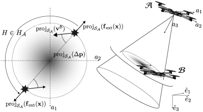
Figure 1: An illustration of Assumption 2 on the downwash function ${\boldsymbol{\mathrm{f}}}_{\mathrm{ext}}(\mathbf{x})$. On the left, we provide two combinations of $(\Delta\mathbf{p},\mathbf{v}^{\mathcal{B}})$ that are related under the rotational equivariance property.

The geometric properties of functions are described in terms of group actions. To be specific, let $G$ be a group and $\mathcal{X}$ be a set. The action of group $G$ on set $\mathcal{X}$ is a mapping $\star:G\times\mathcal{X}\rightarrow\mathcal{X}$ which associates with each group element and set element a corresponding set element. The group action $\star$ must satisfy certain properties [18, 19]. In this case, we say that “$G$ acts on $\mathcal{X}$ according to $\star$.”

For instance, if $G=\mathsf{SO}(2)$ and $\mathcal{X}=\mathbb{R}^{2}$, then $G$ can act on $\mathcal{X}$ according to matrix multiplication: $G_{\omega}\star\mathbf{w}=G_{\omega}\mathbf{w}$, where $G_{\omega}\in\mathsf{SO}(2)$ is the rotation matrix corresponding to the angle $\omega\in[0,2\pi)$ and $\mathbf{w}\in\mathbb{R}^{2}$ is an arbitrary vector.

Using group actions, one can define invariant and equivariant functions:

Definition 1 (Invariance, Equivariance).

Let $G$ be a group and $\mathcal{X},\mathcal{Y}$ be two sets. Suppose that $G$ acts on $\mathcal{X}$ according to $\star_{1}$ and on $\mathcal{Y}$ according to $\star_{2}$.

A function $f:\mathcal{X}\rightarrow\mathcal{Y}$ is invariant with respect to $\star_{1}$ if it satisfies

$$f(x)=f(g\star_{1}x),\quad\forall x\in\mathcal{X},\forall g\in G.$$

$f$ is equivariant with respect to $\star_{1}$ and $\star_{2}$ if it satisfies

$$g\star_{2}f(x)=f(g\star_{1}x),\quad\forall x\in\mathcal{X},\forall g\in G.$$

Intuitively, invariance states that the output of $f$ should be preserved regardless of whether or not $g\in G$ acts on the input. Equivariance, on the other hand, states that $g\in G$ acting on the input $x$ according to $\star_{1}$ is equivalent to $g$ acting on the output of $f$, $f(x)$, according to $\star_{2}$.

III-B Geometric Assumptions on ${\boldsymbol{\mathrm{f}}}_{\mathrm{ext}}$

Now that we have detailed the geometric properties a function may have, we consider the particular structure of the interaction forces $\mathbf{f}_{\text{ext}}(\mathbf{x})$ that Alpha exerts on Bravo.

Foremost, we know that ${\boldsymbol{\mathrm{f}}}_{\mathrm{ext}}(\mathbf{x})$ should not depend on positional shifts in the input space:

Assumption 1 (Translation Invariance).

Define the group $\mathbb{T}$ consisting of all translations in $\mathbb{R}^{3}$. $\mathbb{T}$ is isomorphic to $\mathbb{R}^{3}$. We assume ${\boldsymbol{\mathrm{f}}}_{\mathrm{ext}}(\mathbf{x})$ is invariant with respect to the group action $\mathbf{t}\star_{1}\mathbf{x}=[\mathbf{t}+{\boldsymbol{\mathrm{p}}}^{\mathcal{A}},\mathbf{t}+{\boldsymbol{\mathrm{p}}}^{\mathcal{B}},{\boldsymbol{\mathrm{v}}}^{\mathcal{A}},{\boldsymbol{\mathrm{v}}}^{\mathcal{B}}]$ for $\mathbf{t}\in\mathbb{T}$.

Equivalently, Assumption 1 states that $\mathbf{f}_{\text{ext}}$ must be a function of $\Delta{\boldsymbol{\mathrm{p}}}$, ${\boldsymbol{\mathrm{v}}}^{\mathcal{A}}$, and ${\boldsymbol{\mathrm{v}}}^{\mathcal{B}}$ only. From here on, we will redefine $\mathbf{x}\equiv[\Delta{\boldsymbol{\mathrm{p}}}$, ${\boldsymbol{\mathrm{v}}}^{\mathcal{A}}$, ${\boldsymbol{\mathrm{v}}}^{\mathcal{B}}]\in\mathbb{R}^{9}$. Translation invariance is standard in downwash models [16, 15, 17].

However, beyond translation invariance, previous downwash models have failed to consider the geometry present in ${\boldsymbol{\mathrm{f}}}_{\mathrm{ext}}$. In particular, in many flight regimes, it is reasonable to assume that once the downward direction $a_{3}$ of the “leader” Alpha is fixed, how one defines the north and east directions is arbitrary. This is the subject of the following assumption:

Assumption 2 (Rotational Equivariance).

Define the group $H_{\mathcal{A}}\leq\mathsf{SO}(3)$ containing all rotations that fix $a_{3}$, the down direction in the body frame of Alpha:

$$H_{\mathcal{A}}\!=\!\big{\{}H\in\mathsf{SO}(3)\ |\ \text{proj}_{\mathcal{S}_{\mathcal{A}}^{\perp}}\left(H\mathbf{w}\right)\!=\!\text{proj}_{\mathcal{S}_{\mathcal{A}}^{\perp}}\left(\mathbf{w}\right)\!,\!\forall\mathbf{w}\in\mathbb{R}^{3}\big{\}}.$$ (3)

$H_{\mathcal{A}}$ is isomorphic to the two-dimensional rotation group, $\mathsf{SO}(2)$. Define the action of $H_{\mathcal{A}}$ on the input space by $H\star_{1}\mathbf{x}=[H\Delta\mathbf{p},\mathbf{v}^{\mathcal{A}},H\mathbf{v}^{\mathcal{B}}]$ and on the output space by $H\star_{2}\mathbf{w}=H\mathbf{w},\mathbf{w}\in\mathbb{R}^{3}$ for $H\in H_{\mathcal{A}}$. Then we assume ${\boldsymbol{\mathrm{f}}}_{\mathrm{ext}}={\boldsymbol{\mathrm{f}}}_{\mathrm{ext}}(\mathbf{x})$ is equivariant with respect to these group actions.

This rotational equivariance assumption is illustrated in Figure 1. Intuitively, Assumption 2 states that in the frame of the leader vehicle Alpha, rotating the relative position vector and the velocity vector of Bravo in the $\{a_{1},a_{2}\}$ axes by an angle of $\omega\in[0,2\pi)$ is equivalent to rotating the force vector $\mathbf{f}_{\text{ext}}(\mathbf{x})$ of Bravo by the same angle $\omega$.

We clarify that the true downwash function will not necessarily satisfy Assumption 2 in all cases. This is the case when Alpha’s rotor speeds are highly asymmetric (ex. during aggressive maneuvering) [13]. However, as we will demonstrate in Section V, imposing this geometric prior on the learning algorithm results in significant improvements in sample efficiency without incurring a large bias. This result is in line with recent research [21] suggesting that even when the assumed geometric priors do not exactly match the underlying symmetry (i.e. “approximate” equivariances), they can still yield gains in sample efficiency while outperforming non-equivariant models.

IV Geometry-Aware Learning

Now that we have stated our assumptions on ${\boldsymbol{\mathrm{f}}}_{\mathrm{ext}}(\mathbf{x})$, we encode them as geometric priors in our learning algorithm.

IV-A Rotationally Equivariant Model

In order to present our model for ${\boldsymbol{\mathrm{f}}}_{\mathrm{ext}}(\mathbf{x})$, we first define a feature mapping $h:\mathbb{R}^{9}\rightarrow\mathbb{R}^{6}$

$$h(\mathbf{x})=\bigg{(}\!\frac{\text{proj}_{\mathcal{S}_{\mathcal{A}}}(\Delta{\boldsymbol{\mathrm{p}}})^{\top}\text{proj}_{\mathcal{S}_{\mathcal{A}}}({\boldsymbol{\mathrm{v}}}^{\mathcal{B}})}{\|\text{proj}_{\mathcal{S}_{\mathcal{A}}}(\Delta{\boldsymbol{\mathrm{p}}})\|_{2}\|\text{proj}_{\mathcal{S}_{\mathcal{A}}}({\boldsymbol{\mathrm{v}}}^{\mathcal{B}})\|_{2}},\|\text{proj}_{\mathcal{S}_{\mathcal{A}}}\left(\Delta{\boldsymbol{\mathrm{p}}}\right)\|_{2},$$

$$\|\text{proj}_{\mathcal{S}_{\mathcal{A}}}({\boldsymbol{\mathrm{v}}}^{\mathcal{B}})\|_{2},\left[R_{\mathcal{M}}^{\mathcal{A}}\Delta{\boldsymbol{\mathrm{p}}}\right]_{3},\left[R_{\mathcal{M}}^{\mathcal{A}}{\boldsymbol{\mathrm{v}}}^{\mathcal{B}}\right]_{3},\|\text{proj}_{\mathcal{S}_{\mathcal{A}}}({\boldsymbol{\mathrm{v}}}^{\mathcal{A}})\|_{2}\!\bigg{)}.$$ (4)

The mapping ${\boldsymbol{\mathrm{x}}}\mapsto h({\boldsymbol{\mathrm{x}}})$ transforms each input vector ${\boldsymbol{\mathrm{x}}}$ in Euclidean space into an invariant representation with respect to the action of $H_{\mathcal{A}}$. It does so by separating each of the inputs $\Delta\mathbf{p}$, $\mathbf{v}^{\mathcal{A}}$, and $\mathbf{v}^{\mathcal{B}}$ into their components in the subspaces $\mathcal{S}_{\mathcal{A}}$ and $\mathcal{S}_{\mathcal{A}}^{\perp}$.

In particular, because the components of $\Delta\mathbf{p}$ and $\mathbf{v}^{\mathcal{B}}$ contained in $\mathcal{S}_{\mathcal{A}}^{\perp}$, $\text{proj}_{\mathcal{S}_{\mathcal{A}}^{\perp}}(\Delta\mathbf{p})$ and $\text{proj}_{\mathcal{S}_{\mathcal{A}}^{\perp}}(\mathbf{v}^{\mathcal{B}})$, are unaffected by the action of $H_{\mathcal{A}}$, then our model has the freedom to operate on them arbitrarily. These components can be rewritten in the frame of Alpha as $\left[R_{\mathcal{M}}^{\mathcal{A}}\Delta{\boldsymbol{\mathrm{p}}}\right]_{3}$ and $\left[R_{\mathcal{M}}^{\mathcal{A}}{\boldsymbol{\mathrm{v}}}^{\mathcal{B}}\right]_{3}$. The components contained in $\mathcal{S}_{\mathcal{A}}$, on the other hand, $\text{proj}_{\mathcal{S}_{\mathcal{A}}}(\Delta\mathbf{p})$ and $\text{proj}_{\mathcal{S}_{\mathcal{A}}}(\mathbf{v}^{\mathcal{B}})$, are affected by the action $\star_{1}$ of $H_{\mathcal{A}}$. Therefore, we only consider the magnitudes of these vectors as well as the angles between them [30, 31]. Formal verifications of these statements are given in the proof of Theorem 1.

While the feature mapping (IV-A) we proposed is invariant with respect to the action of $H_{\mathcal{A}}$, we ultimately want our model for ${\boldsymbol{\mathrm{f}}}_{\text{ext}}(\mathbf{x})$ to be equivariant with respect to $\star_{1}$ and $\star_{2}$. We achieve this by taking into account the polar angle that $\text{proj}_{\mathcal{S}_{\mathcal{A}}}(\Delta{\boldsymbol{\mathrm{p}}})$ forms with the positive $a_{1}$ axis in the subspace $\mathcal{S}_{\mathcal{A}}$, which we denote by $\varphi(\mathbf{x})\in[0,2\pi)$.

Now, for any neural network function $f_{\Theta}:\mathbb{R}^{6}\rightarrow\mathbb{R}^{2}$ with parameters $\Theta$, we will approximate the downwash forces $\mathbf{f}_{\text{ext}}$ felt by Bravo as $F_{\Theta}:\mathbb{R}^{9}\rightarrow\mathbb{R}^{3}$:

$$F_{\Theta}(\mathbf{x})\!=\!(R_{\mathcal{M}}^{\mathcal{A}})^{\top}\!\bigg{(}\!\left[f_{\Theta}(h(\mathbf{x}))\right]_{1}\!\cdot\![c(\varphi(\mathbf{x})),s(\varphi(\mathbf{x}))],\left[f_{\Theta}(h(\mathbf{x}))\right]_{2}\!\bigg{)}.$$ (5)

IV-B Proof of Equivariance

Theorem 1.

The model $F_{\Theta}(\mathbf{x})$ proposed in (5) for ${\boldsymbol{\mathrm{f}}}_{\mathrm{ext}}(\mathbf{x})$ satisfies Assumption 2.

Proof.

By Definition 1 of equivariance, we need to prove that for each $H\in H_{\mathcal{A}}$,

$$H\star_{2}F_{\Theta}(\mathbf{x})=F_{\Theta}(H\star_{1}\mathbf{x}),$$

where $\star_{1}$ and $\star_{2}$ are the group actions in Assumption 2.

First, we point out the fact that

$$H_{\mathcal{A}}=\left\{(R_{\mathcal{M}}^{\mathcal{A}})^{\top}\begin{pmatrix}c(\omega)&-s(\omega)&0\\ s(\omega)&c(\omega)&0\\ 0&0&1\end{pmatrix}R_{\mathcal{M}}^{\mathcal{A}}\ \bigg{|}\ \omega\in[0,2\pi)\right\}.$$ (6)

In other words, each $H\in H_{\mathcal{A}}$ can be parameterized by the angle of rotation $\omega\in[0,2\pi)$ about the axis $a_{3}$. Let $H=(R_{\mathcal{M}}^{\mathcal{A}})^{\top}\Omega R_{\mathcal{M}}^{\mathcal{A}}$, where $\Omega$ is the rotation matrix in (6).

As we previously discussed, we will first show that the feature mapping (IV-A) is invariant to the action of $H_{\mathcal{A}}$ on the input space, $\star_{1}$. Since $H$ is a rotation which fixes $a_{3}$, then

$$\left[R_{\mathcal{M}}^{\mathcal{A}}H{\boldsymbol{\mathrm{w}}}\right]_{3}=\left[\Omega R_{\mathcal{M}}^{\mathcal{A}}{\boldsymbol{\mathrm{w}}}\right]_{3}=\left[R_{\mathcal{M}}^{\mathcal{A}}{\boldsymbol{\mathrm{w}}}\right]_{3},\ \forall{\boldsymbol{\mathrm{w}}}\in\mathbb{R}^{3}.$$

Also, notice that

$$R_{\mathcal{M}}^{\mathcal{A}}\text{proj}_{\mathcal{S}_{\mathcal{A}}}(\mathbf{w})=\begin{pmatrix}\mathbb{I}_{2\times 2}&0\\ 0&0\end{pmatrix}R_{\mathcal{M}}^{\mathcal{A}}\mathbf{w}.$$

But for any vector $\mathbf{w}\in\mathbb{R}^{3}$,

$$R_{\mathcal{M}}^{\mathcal{A}}\text{proj}_{\mathcal{S}_{\mathcal{A}}}(H\mathbf{w}) =\begin{pmatrix}\mathbb{I}_{2\times 2}&0\\ 0&0\end{pmatrix}R_{\mathcal{M}}^{\mathcal{A}}H\mathbf{w}$$

$$=\Omega R_{\mathcal{M}}^{\mathcal{A}}\text{proj}_{\mathcal{A}}(\mathbf{w}).$$

Since $\Omega$ and $R_{\mathcal{M}}^{\mathcal{A}}$ are unitary, and the norm and dot product are preserved under unitary transformations, the previous two results imply $h(H\star_{1}\mathbf{x})=h(\mathbf{x})$.

Hence, it only remains to consider the polar angle that $\text{proj}_{\mathcal{S}_{\mathcal{A}}}(H\Delta\mathbf{p})$, or equivalently $R_{\mathcal{M}}^{\mathcal{A}}\text{proj}_{\mathcal{S}_{\mathcal{A}}}(H\Delta\mathbf{p})$, forms with the positive $a_{1}$ axis in $S_{\mathcal{A}}$. But $R_{\mathcal{M}}^{\mathcal{A}}\text{proj}_{\mathcal{A}}(H\Delta\mathbf{p})=\Omega R_{\mathcal{M}}^{\mathcal{A}}\text{proj}_{\mathcal{A}}(\Delta\mathbf{p})$ is just $R_{\mathcal{M}}^{\mathcal{A}}\text{proj}_{\mathcal{A}}(\Delta\mathbf{p})$ rotated by $\omega$. Therefore, we know that

$$\varphi(H\star_{1}\mathbf{x})\equiv\varphi(\mathbf{x})+\omega\quad(\text{mod $2\pi$}).$$

Let $\Omega_{2\times 2}\in\mathbb{R}^{2\times 2}$ be the submatrix formed by the first two rows and columns of $\Omega$. Using our established congruence,

$$\Omega_{2\times 2}[c(\varphi(\mathbf{x})),s(\varphi(\mathbf{x}))] =[c(\varphi(\mathbf{x})+\omega),s(\varphi(\mathbf{x})+\omega)]$$

$$=[c(\varphi(H\star_{1}\mathbf{x})),s(\varphi(H\star_{1}\mathbf{x}))].$$

Altogether, we conclude that

$$F_{\Theta}(H\star_{1}\mathbf{x})$$

$$= (R_{\mathcal{M}}^{\mathcal{A}})^{\top}\!\bigg{(}\!\![f_{\Theta}(h(\mathbf{x}))]_{1}\Omega_{2\times 2}[c(\varphi(\mathbf{x})),s(\varphi(\mathbf{x}))],[f_{\Theta}(h(\mathbf{x}))]_{2}\!\!\bigg{)}$$

$$= (R_{\mathcal{M}}^{\mathcal{A}})^{\top}\Omega\bigg{(}\![f_{\Theta}(h(\mathbf{x}))]_{1}\cdot[c(\varphi(\mathbf{x})),s(\varphi(\mathbf{x}))],[f_{\Theta}(h(\mathbf{x}))]_{2}\!\bigg{)}$$

$$= H(R_{\mathcal{M}}^{\mathcal{A}})^{\top}\!\bigg{(}\![f_{\Theta}(h(\mathbf{x}))]_{1}\cdot[c(\varphi(\mathbf{x})),s(\varphi(\mathbf{x}))],[f_{\Theta}(h(\mathbf{x}))]_{2}\!\bigg{)}$$

$$= H\star_{2}F_{\Theta}(\mathbf{x}).\qed$$

IV-C Shallow Learning

For our training pipeline, we collect time-stamped state and control information from real-world flights with Alpha and Bravo, and compute the input data points ${\boldsymbol{\mathrm{x}}}$ offline. The labels that our model (5) learns to approximate are obtained from the feedback control equation (2), ${\boldsymbol{\mathrm{f}}}_{\mathrm{ext}}={\boldsymbol{\mathrm{a}}}-\boldsymbol{u}(t).$

We choose the neural network $f_{\Theta}$ in (2) to be a shallow network with a single nonlinear activation

$$f_{\Theta}({\boldsymbol{\mathrm{w}}})=W^{(2)}\sigma\left(W^{(1)}{\boldsymbol{\mathrm{w}}}+b^{(1)}\right)+b^{(2)},\quad{\boldsymbol{\mathrm{w}}}\in\mathbb{R}^{6},$$ (7)

where $W^{(1)}\in\mathbb{R}^{32\times 6}$, $b^{(1)}\in\mathbb{R}^{32}$, $W^{(2)}\in\mathbb{R}^{2\times 32}$, $b^{(2)}\in\mathbb{R}^{2}$ are the network parameters $\Theta$ and $\sigma(\cdot)=\max(\cdot,0)$ is the element-wise ReLU nonlinearity. $f_{\Theta}$ is trained to minimize the mean-squared error between the force prediction and label along all three inertial axes $\{\hat{e}_{1},\hat{e}_{2},\hat{e}_{3}\}$.

We justify our choice of a shallow neural network architecture via the $\mathsf{SO}(2)$ invariant feature mapping (IV-A). For a neural network trained only on the raw input data $\mathbf{x}$, the model itself would be responsible for determining the geometries present in ${\boldsymbol{\mathrm{f}}}_{\text{ext}}$. However, for the equivariant model $F_{\Theta}$, the feature mapping (IV-A) encodes these geometries explicitly.

Since our equivariant model is not responsible for learning the geometry of ${\boldsymbol{\mathrm{f}}}_{\text{ext}}$, we can reduce the complexity of $f_{\Theta}$ without sacrificing validation performance. We verify this claim empirically in Section V-B.

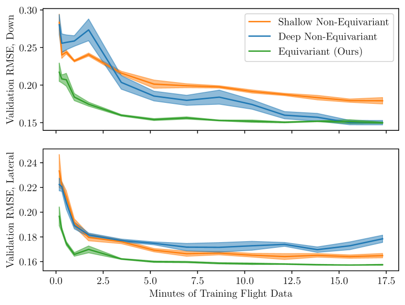
Model	Shallow N-Equiv	Deep N-Equiv	Equivariant (Ours)
Number of Parameters	$323$	$9583$	$258$
Validation RMSE (5 min)	$0.263\pm 0.005$	$0.255\pm 0.005$	$\mathbf{0.222\pm 0.001}$
Validation RMSE (15 min)	$0.243\pm 0.002$	$0.229\pm 0.003$	$\mathbf{0.218\pm 0.002}$
Position Error (lateral) [$\text{\,}\mathrm{m}$]	0.126	0.125	0.104
Position Error (3D) [$\text{\,}\mathrm{m}$]	0.132	0.127	0.106
Velocity Error (lateral) [$\text{\,}\mathrm{m}\mathrm{/}\mathrm{s}$]	0.088	0.089	0.080
Velocity Error (3D) [$\text{\,}\mathrm{m}\mathrm{/}\mathrm{s}$]	0.118	0.095	0.090

Figure 2: Sample Efficiency and Accuracy. Top: A visualization of the validation RMSE of the equivariant and non-equivariant models as a function of the training flight time. For each training time, we compute the average validation RMSE across $5$ trials. Bottom: Summary statistics for the equivariant and non-equivariant models. Position and velocity tracking errors are reported for models trained on the full training dataset.

V Real-world Flight Experiments

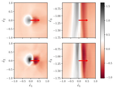
Figure 3: Downward Force Predictions. Downward force predictions [$\text{\,}\mathrm{m}\mathrm{/}\mathrm{s}^{2}$] made by the equivariant model (top) and deep non-equivariant model (bottom). On the left (top-down view), Alpha is hovering $1\text{\,}\mathrm{m}$ above Bravo at $(\hat{e}_{1},\hat{e}_{2})=(0,0)$. On the right (sagittal view), Alpha is hovering $0.1\text{\,}\mathrm{m}$ east of Bravo at $(\hat{e}_{1},\hat{e}_{3})=(0,0)$. In each plot, Bravo is moving with velocity ${\boldsymbol{\mathrm{v}}}^{\mathcal{B}}=[0.5,0,0]^{\top}$.

We conduct studies with our training procedure and present evaluations from real-world flight experiments. All tests are conducted indoors under partially controlled environments to limit the side-effects of external factors.

Consequently, we will consider the special case of the model (5) in which $R_{\mathcal{M}}^{\mathcal{A}}=\mathbb{I}_{3\times 3}$. In other words, we assume Alpha’s frame is a translation of the inertial frame. This special case is realized when Alpha is hovering or its instantaneous state is close to hovering. Since the leader’s velocity is nearly zero, we omit the component $\|\text{proj}_{\mathcal{S}_{\mathcal{A}}}({\boldsymbol{\mathrm{v}}}^{\mathcal{A}})\|_{2}$ from the feature mapping (IV-A).

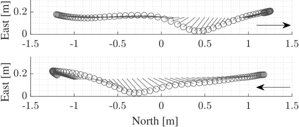
(a) Position tracking errors (solid lines) for Bravo when translating under Alpha. The arrows indicate the direction of travel.

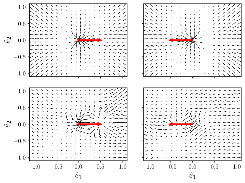
(b) Lateral force predictions made by the equivariant model (top) and deep non-equivariant model (bottom). On the left, Bravo is moving with velocity ${\boldsymbol{\mathrm{v}}}^{\mathcal{B}}=[0.5,0,0]^{\top}$, and on the right it is moving with velocity $-{\boldsymbol{\mathrm{v}}}^{\mathcal{B}}$. Since $\mathsf{SO}(2)$ equivariance is not explicitly imposed in the non-equivariant model, its force predictions do not satisfy the assumed geometry.

Figure 4: Lateral Forces. Force predictions and errors during a transition under Alpha with a vertical separation of $0.8\text{\,}\mathrm{m}$. Alpha is hovering at $(\hat{e}_{1},\hat{e}_{2})=(0,0)$.

V-A Sequential Data Collection

In order to train our model, we first need to collect a dataset of real-world flights. This is a difficult task, since without a compensation model a priori, physical and control limitations will prevent the vehicles from flying in close proximity. To solve this problem, we adopt a sequential approach similar to [16] that splits data collection into different ‘stages’. In stage-0, we fly the vehicles with a relatively large vertical separation, $1.75\text{\,}\mathrm{m}$ to $1.35\text{\,}\mathrm{m}$, so that the forces acting on Bravo can be compensated for by a disturbance-rejecting nominal controller.

This controller has no prior knowledge of the exogenic forces, so it simply relies on its feedback control input, $\boldsymbol{u}(t)$, to track the desired reference trajectories according to (2). However, in regions of strong downwash forces, the measured accelerations, ${\boldsymbol{\mathrm{a}}}$ will not correspond to the desired acceleration input, $\boldsymbol{u}$. These deviations become the computed force labels (represented in mass-normalized acceleration units) for this stage.

After training a stage-0 model using (5), we deploy it online within the control loop such that $\boldsymbol{u}_{\boldsymbol{\mathrm{f}}}$ now provides the feedback regulation. As a result, we can now decrease the separation between the vehicles and obtain a new stage-1 dataset along with its labels (the residual disturbances our stage-0 model is unable to account for). The stage-1 dataset is concatenated with the stage-0 dataset and used to train the stage-1 model.

We repeat this process for a total of three stages, so that at stage-2 the vehicles have a vertical separation of only $\approx$0.5\text{\,}\mathrm{m}$$ (approx. two body-lengths). Our full training dataset corresponds to approximately $17$ minutes of flight data. Note that we can always extract the correct force labels at stage-i by logging the model predictions $F_{\Theta}(\mathbf{x})$ from stage-(i-1) and subtracting these from the control.

V-B Study: Model Training

We first study the effect of geometric priors on the learning algorithm for modelling downwash forces ${\boldsymbol{\mathrm{f}}}_{\mathrm{ext}}(\mathbf{x})$.

Non-equivariant Baselines. In order to analyze the effect of our geometric priors, we must first introduce two models to which we can compare our $\mathsf{SO}(2)$-equivariant model (5). These “non-equivariant” models should not exploit the known geometry of ${\boldsymbol{\mathrm{f}}}_{\mathrm{ext}}$ delineated in Assumption 2.

The first non-equivariant model we propose has the same architecture as the shallow neural network (7), with the exception that the input to the network is $[\Delta{\boldsymbol{\mathrm{p}}},{\boldsymbol{\mathrm{v}}}^{\mathcal{B}}]\in\mathbb{R}^{6}$ rather than invariant feature representation $h({\boldsymbol{\mathrm{x}}})$. Note that ${\boldsymbol{\mathrm{v}}}^{\mathcal{A}}$ is not included because of the near-hover assumption that we specified at the beginning of the section.

We also compare our equivariant model against the SOTA eight-layer, non-equivariant neural network discussed in Section I [16, 15]. During training, we bound the singular values of the weight matrices to be at most $2$. This normalization technique, called “spectral normalization,” constrains the Lipschitz constant of the neural network [16, 15].

Efficiency of Geometric Learning. As we suggested in Section I, the primary benefit of imposing geometric priors on a learning algorithm is that they have been empirically shown to improve sample efficiency [21, 22, 23, 24].

We investigate the sample efficiency of our $\mathsf{SO}(2)$-equivariant downwash model by considering the validation root mean-squared error (RMSE) as a function of the length of our training flights. We shorten the full training dataset by shortening each stage of data collection proportionally (ex. a total training time of three minutes corresponds to one minute of flight for each stage). Our validation dataset is roughly equal in size to the full training dataset.

In Figure 2, we observe that although the validation loss of the shallow non-equivariant network plateaus after approximately $10$ minutes of training flight data, it cannot represent the downward aerodynamic forces as accurately as the other models (i.e. greater bias). Conversely, while the deep non-equivariant network accurately learns the downward forces, it requires much more training data to do so (i.e. lower sample efficiency). Neither non-equivariant model learns the lateral forces as accurately as the equivariant model.

Our equivariant model (5), on the other hand, displays both high sample efficiency and low bias. With only $5$ minutes of flight data, it learns the lateral and downward forces more accurately than both non-equivariant models do with $15$ minutes of data.

Visualizing Downwash Predictions. In Figure 3, we visualize the force predictions that our equivariant model $F_{\Theta}(\mathbf{x})$ makes in the $\hat{e}_{3}$ direction. When Bravo passes through the downwash region of Alpha, there is a highly repeatable pattern in which it is first subjected to a positive force, which pushes it towards the ground, followed by a negative force, which pulls it upwards. The magnitudes of these positive and negative forces are dependent upon (i) Bravo’s speed as it passes through the downwash region, and (ii) the distance of Bravo from Alpha in both $\mathcal{S}_{\mathcal{A}}$ and $\mathcal{S}_{\mathcal{A}}^{\perp}$. Similar patterns have been documented by previous downwash models [16].

From Figure 4(b), we observe that $F_{\Theta}$ also uncovers consistent patterns in the lateral axes $\hat{e}_{1}$ and $\hat{e}_{2}$. When Bravo translates laterally underneath Alpha, it is first pushed radially outwards, then pulled inwards immediately upon passing under Alpha, and lastly, pushed radially outwards once it has passed Alpha. These inwards forces are strongest when Bravo is traveling at a high speed. In Figure 4(a), we show that the model’s predictions are consistent with the observed deviations of Bravo from its trajectory.

We believe that we are the first to demonstrate these lateral force patterns via a machine learning approach.

V-C Real-World Experiments

We evaluate the performance of our trained equivariant model (5) in two real-world experiments, and contrast it against a baseline controller as well as the deep non-equivariant model. Each model is trained on the full training dataset as described in Section V-A.

Our tests use two identical quadrotor platforms that are custom-built using commercial off-the-shelf parts. These span $0.24\text{\,}\mathrm{m}$ on the longest body-diagonal, and weigh $0.65\text{\,}\mathrm{k}\mathrm{g}$ (including batteries). Each platform is equipped with a Raspberry Pi 4B (8GB memory) on which we run our control, estimation and model evaluations. The model-based LQG flight control and estimation (2) is perfomed by Freyja [32], while the neural-network encapsulation is done through PyTorch. The controller and the model evaluations are performed at $50\text{\,}\mathrm{H}\mathrm{z}$ and $45\text{\,}\mathrm{H}\mathrm{z}$ respectively.

Prior to conducting tests with Bravo in motion, we first ensure that a stationary hover under Alpha is stable when the model’s predictions are incorporated into Bravo’s control loop. This is essential to validate empirically that the predictions made by the model do not induce unbounded oscillations on Bravo. The table in Figure 2 lists the quantitative results averaged across all our experiments, compared against baseline methods.

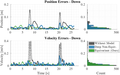
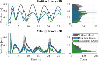
Figure 5: Lemniscate. An evaluation of Bravo’s trajectory tracking performance with Alpha hovering at $\hat{e}_{3}=$-2.5\text{\,}\mathrm{m}$$. The first two rows show the evolution of the position and velocity tracking errors, as well as their distributions. The last two rows show the same statistics in the 3D space. Compared against a baseline controller (without any model) and a non-equivariant model, our model shifts the distribution of full 3D errors in position ($37\text{\,}\mathrm{\char 37\relax}$ reduction in mean error) and velocity ($36\text{\,}\mathrm{\char 37\relax}$ reduction in mean). The non-equivariant model only offers $24\text{\,}\mathrm{\char 37\relax}$ and $28\text{\,}\mathrm{\char 37\relax}$ reductions, respectively.

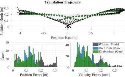
Figure 6: Translation. An evaluation of Bravo’s flight performance over a lateral transect beneath Alpha. This trajectory is replicated from Figure 4(a). Solid black arrows represent the force predictions made by the equivariant model. Applying these predictions, our approach decreases both the mean position and velocity tracking errors by almost $36\text{\,}\mathrm{\char 37\relax}$ (see Figure 2). The gains are greatest in the $\hat{e}_{3}$ axis, where the tracking performance is improved by over $55\text{\,}\mathrm{\char 37\relax}$.

Lemniscate Trajectory. We now evaluate the model deployed in a more dynamic scenario where Bravo is commanded to follow a lemniscate trajectory (‘figure-eight’) under Alpha. This exposes the model to many different regions of the state space, while also requiring Bravo to make continuous changes to its accelerations.

Figure 5 shows tracking results from executing one complete period of this trajectory. We observe that deploying our model produces a significant shift in the distribution of both position and velocity errors. Without any model, Bravo loses vertical position tracking (top row) twice as it makes the two passes directly beneath Alpha, seen near $8\text{\,}\mathrm{s}$ and $20\text{\,}\mathrm{s}$. These spikes, also noticeable as vertical velocity errors (second row), are “absorbed” due to the predictions made by our equivariant model (as well as the baseline deep non-equivariant model). The equivariant model produces an improvement of nearly $51\text{\,}\mathrm{\char 37\relax}$ in both position and velocity tracking, whereas the non-equivariant model is still able to provide almost $36\text{\,}\mathrm{\char 37\relax}$ and $46\text{\,}\mathrm{\char 37\relax}$ improvement, respectively.

Our model’s ability to represent geometric patterns in the lateral plane is also apparent when considering the full 3D errors (third and fourth rows). The non-equivariant model already improves position tracking by $24\text{\,}\mathrm{\char 37\relax}$ ($0.137\text{\,}\mathrm{m}$ from $0.181\text{\,}\mathrm{m}$) and velocity tracking by nearly $28\text{\,}\mathrm{\char 37\relax}$ ($0.091\text{\,}\mathrm{m}\mathrm{/}\mathrm{s}$ from $0.128\text{\,}\mathrm{m}\mathrm{/}\mathrm{s}$). The equivariant model decreases position errors further (down to $0.113\text{\,}\mathrm{m}$, $37\text{\,}\mathrm{\char 37\relax}$ improvement), and also reduces velocity tracking errors (down to $0.081\text{\,}\mathrm{m}\mathrm{/}\mathrm{s}$, a $36\text{\,}\mathrm{\char 37\relax}$ improvement).

Translation Trajectory Next, we perform an analysis of Bravo’s tracking performance and the model’s responses while executing a horizontal transect under Alpha. This trajectory is the same as the one shown in Figure 4(a), and is useful because it drives Bravo rapidly through regions of near-zero to peak disturbances.

Figure 6 illustrates key results from one back-and-forth trajectory parallel to the $\hat{e}_{2}$ axis. $\hat{e}_{1}=0.2$ is fixed, and Bravo is at a fixed vertical separation of $0.6\text{\,}\mathrm{m}$ with Alpha hovering at $\mathbf{p}^{\mathcal{A}}=[0,0,-2.5]$. The first row shows the actual trajectory executed by Bravo with our equivariant model deployed (green circles), with an overlay of the force predictions made by the model (solid black arrows). We first point out that the pattern is similar to the one found in Figure 4(a), but the peak errors have decreased significantly.

The distributions of errors shown in the second row demonstrate that the magnitudes of these predictions are also justified. Even though Bravo is not directly underneath Alpha in these tests, it is still well within Alpha’s downwash region. Across experiments, we observe a reduction in the mean 3D positioning error to $0.098\text{\,}\mathrm{m}$ (from $0.154\text{\,}\mathrm{m}$), corresponding to an improvement of almost $36\text{\,}\mathrm{\char 37\relax}$ (the peak error is also reduced similarly). Velocity tracking error also shows a similar trend, with an average improvement of $34\text{\,}\mathrm{\char 37\relax}$. Considering only the vertical tracking performance in these tests (not shown in figures), these statistics jump to $55\text{\,}\mathrm{\char 37\relax}$ and $49\text{\,}\mathrm{\char 37\relax}$ (for position and velocity, respectively).

VI Conclusion

This article proposes a sample-efficient learning-based approach for modelling the downwash forces produced by a multirotor on another. In comparison to previous learning-based approaches that have tackled this problem, we make the additional assumption that the downwash function is rotationally equivariant about the vertical axis of the leader vehicle. This “geometric prior” that we impose on the learning algorithm allows us to first encode our input data into a lower-dimensional space using an invariant feature mapping, before passing it as the input to a neural network.

Through a number of real-world experiments, we demonstrate that the equivariant model outperforms baseline feedback control as well as SOTA learning-based approaches. The advantage of our equivariant model is greatest in regimes where training data is limited.

In the future, we will further explore the potential of our equivariant model through flight regimes with larger force magnitudes. This includes outdoor flights, where the leader and follower can move at sustained greater speeds. Finally, we will consider how to model the geometries present in a multi-vehicle system. One naïve approach to modelling multi-vehicle downwash would be to employ our two-vehicle model and sum the individual force contributions produced by each multirotor in the system. However, it may be the case that individual downwash fields interact in highly nonlinear ways, in which case a more complex model of the multi-vehicle geometry would be necessary.

References

- [1] J. A. Preiss, W. Honig, G. S. Sukhatme, and N. Ayanian, “Crazyswarm: A large nano-quadcopter swarm,” in IEEE International Conference on Robotics and Automation (ICRA). IEEE, 2017, pp. 3299–3304.
- [2] G. Vásárhelyi, C. Virágh, G. Somorjai, T. Nepusz, A. E. Eiben, and T. Vicsek, “Optimized flocking of autonomous drones in confined environments,” Science Robotics, vol. 3, no. 20, p. eaat3536, 2018.
- [3] M. Turpin, N. Michael, and V. Kumar, “Trajectory design and control for aggressive formation flight with quadrotors,” Autonomous Robots, vol. 33, pp. 143–156, 2012.
- [4] A. Shankar, S. Elbaum, and C. Detweiler, “Dynamic path generation for multirotor aerial docking in forward flight,” in 59th IEEE Conference on Decision and Control (CDC). IEEE, 2020, pp. 1564–1571.
- [5] R. Miyazaki, R. Jiang, H. Paul, K. Ono, and K. Shimonomura, “Airborne docking for multi-rotor aerial manipulations,” in IEEE/RSJ International Conference on Intelligent Robots and Systems (IROS). IEEE, 2018, pp. 4708–4714.
- [6] A. Shankar, S. Elbaum, and C. Detweiler, “Multirotor docking with an airborne platform,” in Experimental Robotics: The 17th International Symposium. Springer, 2021, pp. 47–59.
- [7] S. Yoon, P. V. Diaz, D. D. Boyd Jr, W. M. Chan, and C. R. Theodore, “Computational aerodynamic modeling of small quadcopter vehicles,” in American Helicopter Society (AHS) 73rd Annual Forum, 2017.
- [8] S. Yoon, H. C. Lee, and T. H. Pulliam, “Computational analysis of multi-rotor flows,” in 54th AIAA aerospace sciences meeting, 2016, p. 0812.
- [9] S. Shalev-Shwartz and S. Ben-David, Understanding machine learning: From theory to algorithms. Cambridge university press, 2014.
- [10] S.-J. Chung, A. A. Paranjape, P. Dames, S. Shen, and V. Kumar, “A survey on aerial swarm robotics,” IEEE Transactions on Robotics, vol. 34, no. 4, pp. 837–855, 2018.
- [11] X. Zhou, J. Zhu, H. Zhou, C. Xu, and F. Gao, “Ego-swarm: A fully autonomous and decentralized quadrotor swarm system in cluttered environments,” in 2021 IEEE International Conference on Robotics and Automation (ICRA), 2021, pp. 4101–4107.
- [12] G. Throneberry, C. Hocut, and A. Abdelkefi, “Multi-rotor wake propagation and flow development modeling: A review,” Progress in Aerospace Sciences, vol. 127, p. 100762, 2021. [Online]. Available: https://www.sciencedirect.com/science/article/pii/S0376042121000658
- [13] H. Zhang, Y. Lan, N. Shen, J. Wu, T. Wang, J. Han, and S. Wen, “Numerical analysis of downwash flow field from quad-rotor unmanned aerial vehicles,” International Journal of Precision Agricultural Aviation, vol. 3, no. 4, 2020.
- [14] G. Shi, X. Shi, M. O’Connell, R. Yu, K. Azizzadenesheli, A. Anandkumar, Y. Yue, and S.-J. Chung, “Neural lander: Stable drone landing control using learned dynamics,” in 2019 international conference on robotics and automation (icra). IEEE, 2019, pp. 9784–9790.
- [15] G. Shi, W. Hönig, X. Shi, Y. Yue, and S.-J. Chung, “Neural-swarm2: Planning and control of heterogeneous multirotor swarms using learned interactions,” IEEE Transactions on Robotics, vol. 38, no. 2, pp. 1063–1079, 2021.
- [16] G. Shi, W. Hönig, Y. Yue, and S.-J. Chung, “Neural-swarm: Decentralized close-proximity multirotor control using learned interactions,” in 2020 IEEE International Conference on Robotics and Automation (ICRA). IEEE, 2020, pp. 3241–3247.
- [17] J. Li, L. Han, H. Yu, Y. Lin, Q. Li, and Z. Ren, “Nonlinear mpc for quadrotors in close-proximity flight with neural network downwash prediction,” arXiv preprint arXiv:2304.07794, 2023.
- [18] M. M. Bronstein, J. Bruna, T. Cohen, and P. Veličković, “Geometric deep learning: Grids, groups, graphs, geodesics, and gauges,” arXiv preprint arXiv:2104.13478, 2021.
- [19] C. Esteves, “Theoretical aspects of group equivariant neural networks,” arXiv preprint arXiv:2004.05154, 2020.
- [20] M. M. Bronstein, J. Bruna, Y. LeCun, A. Szlam, and P. Vandergheynst, “Geometric deep learning: going beyond euclidean data,” IEEE Signal Processing Magazine, vol. 34, no. 4, pp. 18–42, 2017.
- [21] D. Wang, J. Y. Park, N. Sortur, L. L. Wong, R. Walters, and R. Platt, “The surprising effectiveness of equivariant models in domains with latent symmetry,” arXiv preprint arXiv:2211.09231, 2022.
- [22] S. Batzner, A. Musaelian, L. Sun, M. Geiger, J. P. Mailoa, M. Kornbluth, N. Molinari, T. E. Smidt, and B. Kozinsky, “-equivariant graph neural networks for data-efficient and accurate interatomic potentials,” Nature communications, vol. 13, no. 1, p. 2453, 2022.
- [23] D. Wang, R. Walters, X. Zhu, and R. Platt, “Equivariant learning in spatial action spaces,” in Conference on Robot Learning. PMLR, 2022, pp. 1713–1723.
- [24] A. K. Mondal, V. Jain, K. Siddiqi, and S. Ravanbakhsh, “Eqr: Equivariant representations for data-efficient reinforcement learning,” in International Conference on Machine Learning. PMLR, 2022, pp. 15 908–15 926.
- [25] B. Yu and T. Lee, “Equivariant reinforcement learning for quadrotor uav,” arXiv preprint arXiv:2206.01233, 2022.
- [26] X. Zhu, D. Wang, O. Biza, G. Su, R. Walters, and R. Platt, “Sample efficient grasp learning using equivariant models,” arXiv preprint arXiv:2202.09468, 2022.
- [27] D. Wang, M. Jia, X. Zhu, R. Walters, and R. Platt, “On-robot learning with equivariant models,” in Conference on robot learning, 2022.
- [28] D. Wang, R. Walters, and R. Platt, “-equivariant reinforcement learning,” arXiv preprint arXiv:2203.04439, 2022.
- [29] P. J. Gorder and R. A. Hess, “Sequential loop closure in design of a robust rotorcraft flight control system,” Journal of guidance, control, and dynamics, vol. 20, no. 6, pp. 1235–1240, 1997.
- [30] J. Gasteiger, J. Groß, and S. Günnemann, “Directional message passing for molecular graphs,” arXiv preprint arXiv:2003.03123, 2020.
- [31] K. T. Schütt, H. E. Sauceda, P.-J. Kindermans, A. Tkatchenko, and K.-R. Müller, “Schnet–a deep learning architecture for molecules and materials,” The Journal of Chemical Physics, vol. 148, no. 24, p. 241722, 2018.
- [32] A. Shankar, S. Elbaum, and C. Detweiler, “Freyja: A full multirotor system for agile & precise outdoor flights,” in IEEE International Conference on Robotics and Automation (ICRA). IEEE, 2021, pp. 217–223.