IDToolkit: A Toolkit for Benchmarking and Developing Inverse Design Algorithms in Nanophotonics

Abstract.

Aiding humans with scientific designs is one of the most exciting of artificial intelligence (AI) and machine learning (ML), due to their potential for the discovery of new drugs, design of new materials and chemical compounds, etc. However, scientific design typically requires complex domain knowledge that is not familiar to AI researchers. Further, scientific studies involve professional skills to perform experiments and evaluations. These obstacles prevent AI researchers from developing specialized methods for scientific designs. To take a step towards easy-to-understand and reproducible research of scientific design, we propose a benchmark for the inverse design of nanophotonic devices, which can be verified computationally and accurately. Specifically, we implemented three different nanophotonic design problems, namely a radiative cooler, a selective emitter for thermophotovoltaics, and structural color filters, all of which are different in design parameter spaces, complexity, and design targets. The benchmark environments are implemented with an open-source simulator. We further implemented 10 different inverse design algorithms and compared them in a reproducible and fair framework. The results revealed the strengths and weaknesses of existing methods, which shed light on several future directions for developing more efficient inverse design algorithms. Our benchmark can also serve as the starting point for more challenging scientific design problems. The code of IDToolkit is available at https://github.com/ThyrixYang/IDToolkit.

1. Introduction

Machine learning for scientific discovery, with the goal of establishing data-driven methods to advance the research and developments, has become an intriguing area attracting a lot of researchers in recent years. (Schmidt et al., 2019; Butler et al., 2018; Reichstein et al., 2019; Choudhary et al., 2022). For example, machine-learning techniques have been successfully applied in biology (Jumper et al., 2021), chemistry (Gómez-Bombarelli et al., 2018), physics(Karagiorgi et al., 2022), nanophotonics(Yang et al., 2023) etc. In the majority of scientific design problems, the performance of a design often necessitates physical experiments to validate its efficacy. This greatly hinders the development and validation of inverse design algorithms. On the contrary, the performance of nanophotonic devices can be verified through computational simulations accurately, enabling a significant acceleration in the verification process and a reduction in associated costs.

Figure 1. The procedure of manually inverse design and our framework of inverse design based on machine learning.

In nanophotonics, inverse design refers to approaches that aim to discover optical structures with fashioned optical properties. Generally, a "forward" procedure means the mapping from the given geometry of a nanophotonic device to the target electromagnetic response. Numerical methods can obtain this mapping process. While an "inverse" procedure indicates a backward process from the target optical response to predict some nanophotonic structures with properties close to the target response. A traditional inverse design process of nanophotonic structures highly rely on the experiments of human experts as depicted in Figure. 1 (a). But this method is hard to design complex nanophotonic structures with a lot of design parameters. Various computational inverse-design methods have been proposed to improve the design efficiency for high-performance nanophotonic devices, such as genetic algorithms (Baumert et al., 1997), and variations of the adjoint method (Lalau-Keraly et al., 2013; Sell et al., 2017; Xiao et al., 2016; Hughes et al., 2018; Mansouree et al., 2021). Among them, the adjoint method, which requires explicit formulation of the underline Maxwell’s equation, is one of the most widely adopted methods in commercial simulation software. However, this method cannot tackle discrete parameters and require a large number of forward simulations, as well as some treatments to jump out of the local minima.(Campbell et al., 2019) Thus, data-driven, problem-agnostic inverse design methods based on machine learning approaches are of particular interest in nanophotonic research in recent years.

However, some prominent obstacles prevent machine learning researchers from developing inverse design algorithms. First, it is not straightforward for computer scientists to understand the specific problems in other scientific areas. The critical issue lies in the formulation of an inverse design problem into a machine learning problem due to the required domain knowledge. Secondly, it is challenging to evaluate the performance of the design. For example, a new design might need to be simulated or produced to measure performance. However, it’s nearly impossible for machine-learning researchers to evaluate by themselves because the evaluation may need professional software, instruments, and skills to operate. These obstacles prevent the machine-learning community from developing practical algorithms independently. Thirdly, most nanophotonic studies did not open-source the implementation of the simulation model and the inverse design algorithms, which further exacerbated the difficulties of reproducing and comparing inverse design algorithms.

Successful benchmarks can directly impel the development of machine learning algorithms. Machine-learning-based data-driven approaches rely on established datasets and benchmarks to develop and evaluate. To name a few, Imagenet(Deng et al., 2009) for image classification, COCO(Lin et al., 2014) for object segmentation, OpenAI Gym(Brockman et al., 2016) and StarCraft(Vinyals et al., 2017) for reinforcement learning, Movielens(Harper and Konstan, 2016) for recommender systems, etc. There are a few inverse design benchmarks that rely on substitute models to evaluate the performance(Ren et al., 2020, 2022). However, the simulation error of the inverse-designed parameters turned out to be significantly larger than predicted by the substitute model(Deng et al., 2021), which indicates that direct evaluation with a simulator is necessary for developing and evaluating accurate inverse design algorithms. As far as we know, there lacks an inverse design benchmark with direct interaction with physical simulators.

In this work, we introduce a benchmark for inverse design, which consists of three different nanophotonic designs from practical applications. We implemented the simulation models of all three problems with MEEP(mee, 2010), which is open-source and scalable on Linux clusters. We implement 10 different inverse design algorithms, and conducted extensive experiments. The experimental results indicate that the performances are related to the properties of specific problems and algorithms. For example, a tree-based optimization algorithm performs better in design problems with discrete parameters; gradient descent method performs better in scenarios with a large amount of training data and continuous parameters. In addition, we point out several promising research directions based on the experimental results and our experience. Our benchmark can also serve as the starting point for other challenging scientific design problems, such as chemical design(Gómez-Bombarelli et al., 2018). The algorithms and interfaces implemented in the benchmark can also be adapted to different design problems. Our contribution can be summarized as follows:

• We propose three distinct inverse design problems selected from practical applications, which have different search spaces and various difficulties. These problems can be used to develop and evaluate inverse design algorithms in a unified framework.

• We implemented and compared 10 different inverse design methods that cover most of the existing approaches in inverse design literature. We conduct extensive experiments to compare the algorithms from different perspectives, which reveals the strength and weaknesses of different algorithms.

• Based on our experimental results and our analysis of the inverse design problems and algorithms, we point out several future directions for developing efficient inverse design algorithms with our benchmark.

2. Background

In inverse design problems, we are supposed to have a forward simulation interface, which takes the design parameters $\mathbf{x}$ as input and output a vector $\mathbf{y}$ that corresponds to some concerned properties that are related to the performance. Generally, a forward simulation procedure can be denoted as $\mathcal{F}(\mathbf{x})=\mathbf{y}$, where $\mathbf{x}=\{x_{0},...,x_{n-1}\}$ denotes $n$ design parameters, $\mathbf{y}=\{y_{0},...,y_{m-1}\}$ denotes $m$ design targets. The design parameters $\mathbf{x}_{i}$ may be continuous or discrete, for example, in the color filter problem, we need to design the material and thickness of a specific layer, where the material is a discrete design parameter that can be chosen within a pool, and the thickness is a continuous design parameter. The design targets $\mathbf{y}$ are continuous in our problems.

The goal of inverse design is to find the best design parameter $x^{*}$ that

(1) $$\mathbf{x}^{*}=\min_{\mathbf{x}} \mathcal{L}(\mathcal{F}(\mathbf{x}),\mathbf{y}_{\text{target}})$$

s.t. $$\mathbf{x}\in\mathcal{D}$$

where $\mathcal{D}$ is the feasible design parameter space. $\mathcal{L}(\mathbf{y},\mathbf{y}^{\prime})$ is a function that measures the difference between $\mathbf{y}$ and $\mathbf{y}^{\prime}$. The search space $\mathcal{D}$ of design parameters can be complex. For example, in the TPV inverse design problem, the feasible range of $\mathbf{x}_{3}$ is determined by the value of $\mathbf{x}_{0}$. Typically, perfect solution with $\mathcal{F}(\mathbf{x})=\mathbf{y}_{target}$ does not exist, which further increases the difficulty.

3. The benchmark

In this section, we provide a brief overview of the composition of input variable $\mathbf{x}$ and output variable $\mathbf{y}$ for the three mentioned problems. A detailed description of the physical problems is presented in the appendix.

3.1. Multi-layer Optical Thin Films (MOTFs)

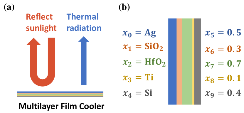
Figure 2. Depiction of MOTFs: (a) How a MOTFs works. (b) The design parameters of a MOTFs with 5 layers.

Multilayer optical thin films (MOTFs) are simple structures with many layers of optical films stacked together. They have been widely used in many optical applications to achieve specific optical properties, such as antireflective coating (ARC), distributed Bragg reflector (DBR), energy harvesting, and radiative cooling. To optimize an MOTF cooler with ideal properties, we implement a simulator with 7 different dispersive materials. We set the layer number to 10, which provides a fairly large search space and enough flexibility (Raman et al. (2014) proposes a 10 layer design). The layer number can be easily increased if necessary and less layer number can be obtained through setting some layer thicknesses to 0. In addition, the MOTF cooler design problem has both discrete (material type) and continuous (layer thickness) variables, and the effective number of variables is not fixed. The design parameters of a multilayer film cooler is depicted in Figure. 2 (b). Specifically, assuming there $k$ different layers, the design parameter $\mathbf{x}_{0},...,\mathbf{x}_{k-1}$ determine the the material used in the 1st to the kth layer respectively; the design parameter $\mathbf{x}_{k},...,\mathbf{x}_{2k-1}$ define the thicknesses of the 1st to kth layer, respectively. The material can be set to 7 different categorical values $\mathbf{x}_{i}\in\{ZnO,AlN,Al_{2}O_{3},MgF_{2},SiO_{2},TiO_{2},SiC\},0<i<k$. The layer thicknesses can be set to $\mathbf{x}_{i}\in[0,1],k\leq i<2k$. The response $\mathbf{y}$ is a 2001-dimensional real-valued vector.

3.2. Thermophotovoltaics (TPV)

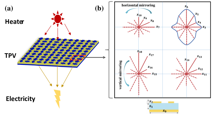
Figure 3. Depiction of the TPV problem: (a) How TPV energy conversion works. (b) The design parameters of TPV.

One of the promising applications of metamaterials is for energy harvesting using thermophotovoltaic (TPV) cells. We adopt a popular design scheme of metamaterial with the unit cell consisting of a bottom metal substrate and top plasmonic structures spaced by a dielectric layer, as depicted in Figure. 3 (a). Tungsten (W) was selected for both the bottom metallic layer and top structural layer. Alumina (Al₂O₃) is used as the dielectric spacer with the thickness $\mathbf{x}_{1}$ varying in the range 30 nm to 130 nm. The dielectric spacer is $\mathbf{x}_{0}$ corresponds the size of a cell, and $\mathbf{x}_{2}$ are the thickness of top metal layer. Considering the feasibility of fabricating the designed TPV, the cells should be single-connected and have smooth edges. To this end, we propose to utilize the B-Spline method to generate the shape of the cells. The control points of B-Spline are defined by the design parameters $\mathbf{x}_{3},...,\mathbf{x}_{18}$. To further increase the flexibility, we use 4 sub-cells in a single cell as depicted in Figure. 3 (b). Each sub-cell is controlled by 4 control points and is reflected vertically and horizontally to produce a symmetrical shape. We set $\mathbf{x}_{0}\in[350,500]$, $\mathbf{x}_{2}\in[10,80]$ and $\mathbf{x}_{i}\in[40,\frac{\mathbf{x}_{0}}{2}],2<i<19$. The constraint on $\mathbf{x}_{i},2<i<19$ is because the radius must be smaller than $\frac{1}{2}$ of the cell size $\mathbf{x}_{0}$ so that the sub-cells will not overlap. The response $\mathbf{y}$ is a 500-dimensional real-valued vector.

3.3. Structural color filter (SCF)

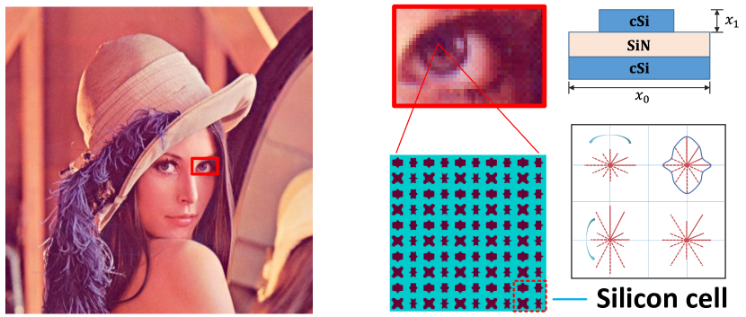
Figure 4. A schematic introduction of high-DPI printing with silicon colors. Each pixel is implemeted by a specific nanostructure cell, where the size of each cell is set to 150nm-350nm.

Structural color filtering (SCF) using plasmonic and dielectric metamaterials has enabled tremendous potential for coloring applications, including passive color display, information storage, Bayer filtering, etc. (Kumar et al., 2012; Duan et al., 2017; Zou et al., 2022; Song et al., 2022; Ma et al., 2022; Gao et al., 2019) In this benchmark, we modeled the color filter using an arrayed silicon metasurface, whose supercell consists of four pillars sitting on a 70-nm SiN₃ thin film, which is supported by a silicon substrate. The cell size is controlled by the parameter $\mathbf{x}_{0}$, and the height of the four pillars are the same and are varied as the parameter of $\mathbf{x}_{1}$. The shapes of the four silicon pillars are independently generated with parameters $\mathbf{x}_{2},...,\mathbf{x}_{17}$, which are similar to the TPV problem. To obtain a structural color filter, we need to design a color palette where each color is implemented with a specific nanostructure. The response $\mathbf{y}$ is a 3-dimensional real-valued vector corresponding to the colors. The inverse design problem is to find nanostructures that match with the colors that are to be printed.

3.4. Speed of the simulator

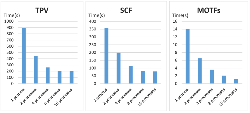
Figure 5. Accelerating simulation by multiprocessing parallelizing.

The speed of the environment is a critical factor for a benchmark. On the one hand, we want the problems to be practical and challenging; on the other hand, we want to evaluate the designs as fast as possible to accelerate the procedure of developing and testing new algorithms. We evaluate the speed of simulating 100 design parameters with our framework, and the results are depicted in Figure. 5. Specifically, we use 2 Intel(R) Xeon(R) Silver 4110 CPUs, each with 8 physical cores, and its base frequency is 2.10 GHz. We evaluate the average time for calculating the results with 1 to 16 processes, respectively. With 1 process, the average time of TPV, SCF, and MOTFs are 894s, 359s, and 14s, respectively. With 16 processes, the average time is 203s, 78s, and 1.2s, respectively. By multiprocessing simulation, we can speed up the calculation by 4.4, 4.6, and 11.6 times faster. Practically, we can use more CPUs in a cluster to further speed up calculation. Thus, the calculation speed of the proposed problems are sufficient for benchmark novel inverse design algorithms. We suggest using the multilayer cooler problem to develop algorithms with faster evaluation procedures, then use TPV and silicon color problems for evaluation on more challenging design problems.

3.5. Comparing to other scientific design problems

The performance of the nanophotonic inverse design can be accurately estimated by our simulator. The performance of nanophotonic devices can be evaluated by the finite-difference time-domain (FDTD) method with theoretically guaranteed precision. This contrasts with drug and chemical designs, where only a heuristic score function is available(Gao et al., 2022). For example, the QED function used in (Gao et al., 2022) can only predict if a chemical is "drug-like." The chemical found is not necessarily a real drug, let alone any performance guarantee. So in these problems, physical experiments are necessary to evaluate the actual design performance. On the contrary, the performance of nanophotonic devices can be accurately estimated with a dedicated FDTD simulator (e.g., MEEP), which means we can evaluate the performance of inverse design algorithms much more accurately without physical experiments. We provide more details in Appendix. We think such a precision guarantee makes our benchmark outstanding at reflecting the performance of general inverse design algorithms in the real world.

The surrogate models trained with machine learning methods may not be accurate evaluation functions. Many existing benchmarks use deep neural networks to construct surrogate simulators. For example, MLP surrogates are used in (Ren et al., 2020); SVM and random forest are used in DRD2, GSK3$\beta$, JNK3(Gao et al., 2022). Such benchmarks are much easier to implement than ours: Generate a dataset with dedicated software, then train an off-the-shelf deep model (MLP, CNN, GNN, Transformer, etc.) will do the job. There is no need to consider the interactions and interfaces of the simulator, which is usually more complicated. However, such surrogates may not reflect the inverse design performance accurately (compared with the physical simulator): While machine learning models typically have high precision on the training and testing dataset generated from the same distribution, the precision drops significantly on the generated designs(Deng et al., 2021). We attribute this performance drop to the fact that the designed parameters are indeed out-of-distribution (OOD) samples, which breaks the generalization guarantee of the learning-based estimators. Thus, our physical simulator is necessary for an accurate evaluation of nanophotonic inverse design methods.

4. Implemented Algorithms

We implement 10 different inverse design methods that cover most categories occurred in literature. We divide the methods into iterative optimizers and deep inverse design methods.

4.1. Iterative optimizers

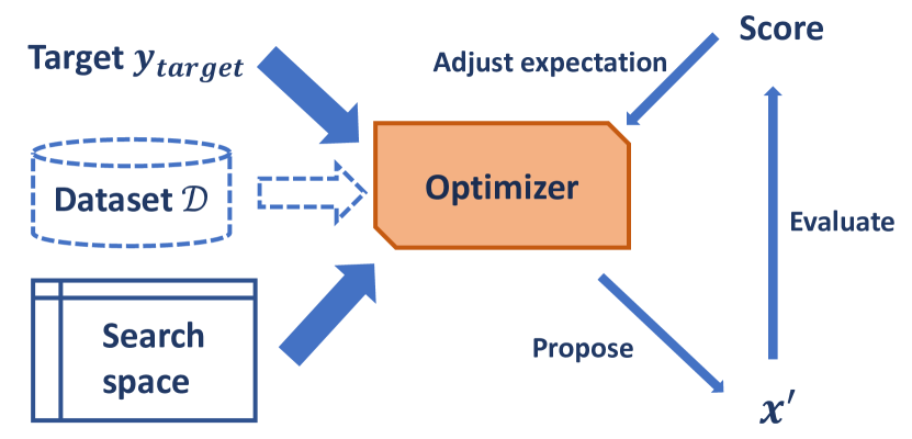
Figure 6. Iterative optimizer.

As depicted in Figure. 6, iterative optimizers work like human experts. The optimizer receives a design target, a specification of search space, and a dataset containing some promising design is optional. Based on the current belief of the search space, the optimizer produces several design parameters $\mathbf{x}^{\prime}$ that are considered promising. The design parameters $\mathbf{x}^{\prime}$ will be evaluated and produce a score, which indicates the performance of this design parameter. The optimizer needs to interact with the simulator to obtain a performance score $\mathcal{S}(\mathbf{x}^{\prime})$. The design parameter $\mathbf{x}^{\prime}$ and the score are fed to the optimizer to adjust the belief of the optimizer. Then, the optimizer generates new design parameters that are considered promising. The whole procedure iterates until satisfactory results are obtained. The iterative optimizers replace expert efforts in analyzing and producing new design parameters. The design procedure can be fully automated.

The experts may also suggest some promising design parameters to the optimizer. Therefore, these methods are highly flexible and can be used to aid manual design. There are also some downsides to iterative optimizers. The iterative optimizer can only design a design target at one time, which will be too time-consuming for inverse design problems with many design targets, such as SCF. The training time and inference time of machine-learning-based optimizers such as Bayesian optimizer scales as $O(n^{3})$ where $n$ is the number of explored data points. Some iterative optimization methods are designed to support discrete design parameters, such as TPE, SRACOS, and ES. This is an important advantage since most of the inverse design problems are involved with some discrete variables such as material type or layer number.

We implement the following iterative optimization methods:

• Random search (RS): The simple but widely used hyper-parameter search method which randomly selects design parameters within the parameter space.

• Sequential randomized coordinate shrinking (SRACOS)(Hu et al., 2017): The SRACOS algorithm trains a classifier to classify good parameters with larger scores and bad parameters with smaller scores. Then, the algorithm draws samples from the parameter space uniformly and select good parameters with the trained classifier as its proposal. The evaluated parameters are inserted into the training dataset to improve the classifier, and new proposals are generated. We implement SRACOS with ZoOpt(Liu et al., 2018a).

• Bayesian Optimization (BO)(Snoek et al., 2012; Dong et al., 2023): The Bayesian optimization method trains a model with a Bayesian method, typically a Gaussian process, which could learn the probability distribution of the score $p(\mathcal{S(\mathbf{x})}|\mathbf{x})$. With the probability information, BO algorithms can evaluate how likely a parameter may improve the score. Then, promising parameters are selected to be evaluated. We implement BO with the BayesOpt library (Martinez-Cantin, 2014).

• Tree-structured Parzen Estimator Approach (TPE) (Bergstra et al., 2011; Lei et al., 2021): Instead of modeling $p(\mathcal{S(\mathbf{x})}|\mathbf{x})$ directly, TPE models $p(\mathbf{x}|\mathcal{S(\mathbf{x})})$ and $p(\mathcal{S(\mathbf{x})})$ with a tree-structured estimator. We implement the TPE method with Hyperopt(Bergstra et al., 2013b, a).

• Evolution Strategy (ES)(Auger, 2009; Deng et al., 2022): Evolution strategies are a set of algorithms that gradually modify current solutions with heuristic methods. We implement a representative ES algorithm called the one-plus-one (1+1) algorithm with implementation from Nevergrad(Rapin and Teytaud, 2018).

4.2. Deep inverse design methods

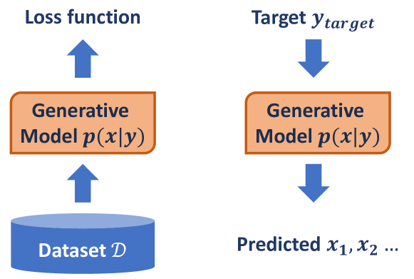
Figure 7. Deep inverse design method.

With the prosperity of deep learning, deep-learning-based methods are adopted to inverse design problems(Molesky et al., 2018), such as VAE(Ma et al., 2019), GAN(Liu et al., 2018c), AAE(Kudyshev et al., 2020), etc. The typical procedure of deep learning-based inverse design methods is depicted in Figure. 7. The deep learning methods are trained to minimize specific loss functions. The trained model can predict design parameters given a design target. Some deep learning methods can produce multiple design parameters $\mathbf{x}_{1},\mathbf{x}_{2},...,\mathbf{x}_{n}$ from $p(\mathbf{x}|\mathbf{y}_{target})$, which is more reasonable since the best design parameter may not be unique.

There are two outstanding advantages of deep learning methods. First, the inference of deep-learning-based methods is typically much faster than iterative optimizers, which enables efficient design of many different design targets. The design for different targets can be parallelized to improve speed further. Secondly, since the prosperity of deep learning methods, the accuracy of neural networks significantly outperforms traditional learning methods on various applications. Deep-learning-based methods can benefit from the progress of neural network architectures directly and lead to better performance.

There are also some disadvantages. First, Deep learning methods have large amounts of parameters, which requires a large amount of data to train. However, in inverse design problems, generating a dataset is typically time-consuming. Thus, the amount of data is a critical bottleneck in the performance of deep learning methods. Secondly, the training time for deep learning methods is long, so it is not easy to add new training data during design like iterative optimization methods, which lacks the ability to improve the model. Thirdly, deep learning methods only work for continuous variables currently, but does not well suit discrete variables.

• Inverse Model (IM)(Liu et al., 2018b): The most straightforward method is to train an inverse model that predicts design parameters given the design target. There is an obvious drawback to this method: there may be multiple different design parameters that lead to the same or similar response. This method will fail to learn the correct design parameter if the solution is not unique.

• Gradient Descent (GD)(Ren et al., 2020; Deng et al., 2021): We can train a forward model $f(x)=\mathcal{F}(x)$ to replace the simulator $\mathcal{F}$. Then, we can use this substitute forward model to find a good solution. If the forward model is differentiable, and the derivatives with respect to the input design parameters are easy to solve, we can apply gradient descent to maximize the performance score directly. In this GD method, we train an MLP as the forward model.

• Tandem(Liu et al., 2018b): Tandem has a forward model and a prediction model. The forward model predicts the response $\mathbf{y}=f(\mathbf{x})$ given the design parameters $\mathbf{x}$ as in GD. Different from GD, Tandem proposes a prediction model $\mathbf{x}^{\prime}=g(\mathbf{y})$ to predict the design parameters directly. The prediction model is trained with cycle loss to make sure that $f(g(\mathbf{y}))\approx\mathbf{y}$ while keep the forward model $f$ fixed.

• Conditional Generative Adversarial Networks (CGAN)(Goodfellow et al., 2014; Mirza and Osindero, 2014; Dan et al., 2020; Kiani et al., 2022): Generative adversarial networks (GAN) have a generator network and a discriminator network. The discriminator network discriminates between real data and generated data. The generator is trained to cheat the discriminator. The two networks are trained alternatively. Theoretically, a GAN will converge to the data distribution $p(x)$. Here we use conditional GAN (CGAN) to learn the conditional distribution $p(\mathbf{x}|\mathbf{y})$.

• Conditional Variational Auto-Encoder (CVAE) (Sohn et al., 2015; Lee and Min, 2022): Variational Auto-Encoders (VAE) have an encoder network that models $p(z|x)$ and a decoder network which models $p(x|z)$, where $z$ is a latent variable that has a simple prior distribution, typically isotropic Gaussian $\mathcal{N}(0,I)$. The VAE maximizes an evidence lower-bound (ELBO) of the log-likelihood $\sum\log p(x)$ during training. After training, the decoder can be used to sample design parameters from $p(x)$ with $z\sim\mathcal{N}(0,I)$ and $x\sim p(x|z)$. Here we adopt conditional variational auto-encoder (CVAE) to train a model of the conditional distribution $p(\mathbf{x}|\mathbf{y})$.

All the methods are implemented using Pytorch(Paszke et al., 2019) within the ray framework(Liaw et al., 2018). Because of the page limit, more details and codes are provided in the Appendix.

5. Experiments

5.1. Dataset

We generate datasets with uniform sampling from the design parameter spaces. Specifically, we sample from $\mathcal{U}(x_{min},x_{max})$ for a continuous design parameter $x$ with maximum value $x_{max}$ and minimum value $x_{min}$. For a discrete variable $x\in\{c_{0},...,c_{k-1}\}$ where $c_{i}$ denotes a categorical value, e.g., material name in the multilayer film problem, the value of $x$ is chosen uniformly from all the $k$ different values with probability $\frac{1}{k}$. The statistics of the three datasets are summarized in Table. (1).

Table 1. Statistics of datasets

	Dataset size	# Input	# Output
MOTFs	60700	20 (80)	2001
TPV	69600	19	500
SCF	25500	18	3

The input of the multilayer film problem consists of 10 categorical parameters (material) and 10 numerical parameters (layer thickness). Some methods such as TPE and ES have direct support for categorical variables, so we use the 20 parameters as inputs directly. For forward prediction tasks, the categorical variables are transformed to their one-hot encodings, so we have $7*10+10=80$ inputs since there are 7 different materials the multilayer film problem.

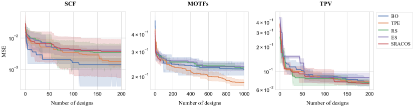
Figure 8. Benchmark on the inverse design tasks without training data.

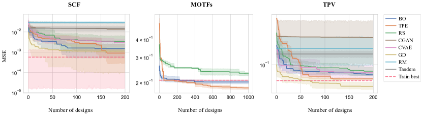
Figure 9. Benchmark the inverse design tasks using all the training data.

We split 90% as the training dataset and 10% as the testing dataset. The testing dataset serves as testing data for forward prediction tasks and inverse design tasks with IID (independent and identically distributed) targets, as described in Section. 5.3 in detail. We further split 90% from the training dataset to train the deep inverse design methods and the forward prediction methods; the left 10% is used for validation. The interactive optimization methods generally do not have a training stage, but they may accept a small collection of suggested design parameters to be tried at first. So we select the 100 best design parameters with the highest scores from the training dataset as the suggested design parameters. It’s also possible to pass the whole dataset to the optimizers. However, the speed is extremely slow since the optimization methods are not designed for large-scale training, and the computational complexity may also be an obstacle for, e.g., Bayesian optimization, which has $O(N^{3})$ time complexity where $N$ is the number of processed data points.

5.2. Inverse Design with Real Targets

All three inverse design problems have pre-defined design targets, which align with their real-world applications. The goal of inverse design is to find design parameters that can produce a response that is as close to the design target as possible. In our experiments, we use the mean squared error (MSE) as the performance measure. Specifically, the performance of a design parameter $\mathbf{x}$ is calculated as follows:

(2) $$\mathcal{L}(\mathcal{F}(\mathbf{x}),\mathbf{y}_{target})=\sum_{j}^{m}({\mathbf{y}_{target}}_{j}-\mathcal{F}(\mathbf{x})_{j})^{2}$$

In the following inverse design benchmarks, we set the number of designs that can be tried by each algorithm to 200, 200, and 1000 in TPV, SCF, and MOTFs, respectively. All the algorithms are run 5 times with different random seeds, we plot the mean value and its 95% confidence interval.

5.2.1. Zero training

The ideal work procedure of an inverse design method is to take the design target as input, and optimize the MSE in a fully automated way without any initial training data. We call this the zero training benchmark. All the iterative optimization methods are designed to work in zero training cases; all the deep learning methods can not work without training data. So we only compare iterative optimization methods in this benchmark. The results are depicted in Figure. 8.

We have the following conclusions

1. The TPE and BO algorithms perform similarly well on the SCF problem, outperforming other algorithms by a large gap. The target space of the silicon color problem is simpler (the dimension of $\mathbf{y}$ is 3) than the other two problems, which enables the probability estimation to be more accurate. Thus, the search algorithms based on probability work better.

2. The TPE algorithm performs best on the MOTFs problem, while other algorithms perform similarly. There are discrete variables in the MOTFs problem, which can be modeled better with tree-structured methods such as TPE.

3. In the TPV problem, all the algorithms perform similarly, as well as the random search method. The TPV problem is intrinsically more complex than the other two problems since all the algorithms cannot find search directions better than random search within 200 trials.

5.2.2. Full train

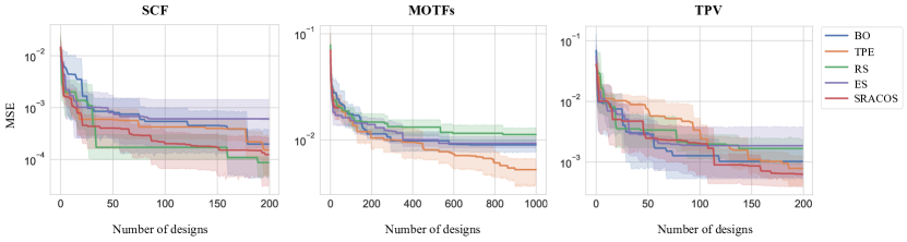
Figure 10. Benchmark on the inverse design tasks with IID-generated targets. The training dataset is not used.

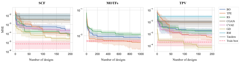
Figure 11. Benchmark on the inverse design tasks with IID-generated targets. All the training dataset is used.

Typically, generating a dataset with random sampling requires considerable computational resources. In this benchmark, we compare the performance of inverse design methods that are trained on the whole training dataset. The results are depicted in Figure. 9. We also plot the performance of the best design parameter within the training dataset (denoted as Train best in dashed line), which also tends to be a reasonably strong baseline.

We have the following observations and conclusions:

1. In our benchmark results, all of the algorithms struggle to make further progress beyond the best training design within limited trials. None of the algorithms exceed the train-best in SCF; TPE is the only method that makes significant progress in MOTFs; GD is the only method that exceeds the train-best in TPV.

2. The train-best design of silicon color is good enough (MSE < $10^{-3}$), which makes it hard to make further improvements. How to make further progress upon high-precision baselines is a good problem for future research.

3. The TPE method can learn meaningful information from training data and produce promising design parameters for optimization with discrete variables.

4. Although TPV is a hard problem, GD can find better design parameters within 200 trials, which indicates that deep models can learn better searching directions of the problem using sufficient training data.

5.3. Inverse Design with IID Targets

The inverse design with real targets is a real-world problem, but may not be an ideal benchmark problem. There are several reasons: First, the perfect design parameter $\mathbf{x}^{*}$ with $\mathcal{F}(\mathbf{x}^{*})=\mathbf{y}_{\text{target}}$ may not exist. Indeed, a perfect design with optimal performance does not exist in most real-world problems, which is simply because of the limitation of physical constraints. So we cannot evaluate how close we are to the best possible solution. Secondly, the performance of the inverse design on the IID targets may serve as an upper bound for the performance on the real target. Indeed, the real targets are out-of-distribution (OOD) data, which are much harder than the IID-generated (in-distribution) targets. Thirdly, the IID assumption is the cornerstone of most machine learning methods and may provide better theoretical properties for further analysis. Thus, the performance of the inverse design method with IID targets is of particular interest for developing and evaluating inverse design algorithms. We sample 5 random design parameters $\mathbf{x}$, then calculate their responses $\mathbf{y}$. These responses are used as IID design targets, which are guaranteed to be realizable in our design parameter space.

The results without training data are depicted in Figure. 10, and the results using all the training data are depicted in Figure. 11. We have the following observations and conclusions:

1. Design for the IID targets is a much easier task since it can intuitively lead to much lower MSE.

2. The performance on the SCF problem is very different from the case with real targets. Thus, the evaluation with IID targets cannot substitute the evaluation with real targets in the SCF problem.

3. The conclusion on the MOTFs problem is similar to results with real targets: TPE is the best-performing method. The conclusion on the TPV problem is also similar to evaluating with the real targets that GD is the best-performing method. This indicates that we may replace real targets with IID targets on specific problems.

6. Related Work

Ardizzone et al. (2019) and Kruse et al. (2021) propose several simple physical problems to evaluate the performance of inverse probability density estimation. However, the physical problems are too simple compared to real-world inverse design problems.

Almost all the research in traditional photics and material science are not open-source(Baumert et al., 1997; Lalau-Keraly et al., 2013; Sell et al., 2017; Xiao et al., 2016; Hughes et al., 2018; Mansouree et al., 2021; Campbell et al., 2019). Yeung et al. (2022) proposes a toolkit for inverse design problems that relies on MATLAB and Lumerical. A prominent difficulty to develop open-source benchmarks on inverse design problems lies in that the modeling is typically implemented using expensive commercial software such as CST, COMSOL, MATLAB, and Lumerical

To side-step such difficulty, several benchmarks have been proposed to substitute simulators with machine learning models trained on a randomly generated dataset(Ren et al., 2020, 2022; Yang et al., 2022). However, there is a significant gap between the predicted performance by the surrogate model and the accurate simulators.(Deng et al., 2021) Surrogate models are generally trained and validated on independent and identically distributed (IID) data, while the inverse-designed parameters are typically non-IID. This discrepancy could lead to misleading benchmark conclusions. To the best of our knowledge, no one has provided an open-source benchmark for inverse design problems with direct access to an accurate simulator. And our benchmark is also fast, reproducible, scalable, and extensible.

7. Future Directions

7.1. Combination of deep learning and interactive optimization

As our comparison at Section. 5, the deep-learning-based methods have better performance on big data and continuous variables, and the iterative optimization methods can tackle discrete variables and start working without training data. We suggest dimension reduction and learning to optimize to combine their advantages.

Dimension reduction. It is known that black-box optimizer will be less effective on high-dimensional optimization(Moriconi et al., 2020). The reason is that the black-box optimization method has little knowledge of the underline structure of the problem, which makes the search inefficient on high-dimensional problems. If we can reduce the dimension of the original problem to a low-dimension space(Wang et al., 2004), the performance of the interactive optimization methods may be improved. A similar idea has been explored by Moriconi et al. (2020), where a multilayer network with sigmoid activation is used to reduce dimension. We believe there is still room for further improvements with the development of dimension reduction methods in recent years.

Learning to optimize. The interactive optimization problem can be seen as a decision-making problem: at each step, the algorithm needs to decide what is the next design parameter to be evaluated based on previous observations. After receiving the score, the optimizer needs to adjust the next design parameters to achieve better performance. Such a decision-making procedure is similar to reinforcement learning, where the policy network should learn to make optimal actions facing different environment states(Arulkumaran et al., 2017). There are also some related topics on learning to optimize neural networks(Chen et al., 2021). However, these learning-based methods require gradients of the objective, which is not available in inverse design problems. Because of its flexibility and data efficiency, learning-based optimization is another promising direction of inverse design algorithms.

7.2. Better forward model and search algorithms

Developing better forward model. One of the reasons for the success of deep learning can be attributed to the ability to learn high-level representation from complex structured data. For example, recent deep learning methods can learn from graph data (there are relations between data points)(Wu et al., 2021), multi-modal data (e.g., data consists of images, videos, texts, etc.)(Baltrusaitis et al., 2019), time series (the concerned value varies along with time)(Lim and Zohren, 2020), etc. Such complex data structures also exist in inverse design problems, and the prediction performances vary by methods and problems. Thus, adopting cutting-edge deep learning methods will lead to better performance of the forward model and enables working with more complex problems.

Search algorithms on substitute model. A straightforward inverse design method is to train a forward model, then use this substitute model to accelerate the design procedure. The forward model can be used to evaluate a design parameter’s performance. We can also utilize the information (e.g., gradients with respect to design parameters) learned by the model to accelerate the optimization of the design parameters. However, as the inverse design problems are typically non-convex, thus, gradient descent is not guaranteed to converge to global minima. And for discrete variables or graph-structured variables, the gradient information is not available. Thus, better search algorithms for efficient optimization of the forward model is necessary for the efficient inverse design.

7.3. Better work with human prior and human in loop

How to incorporate human knowledge has become an important topic in machine learning with the name "human-in-the-loop"(Wu et al., 2022), which aligns with the needs of inverse design problems.

We suggest that how to utilize human knowledge is critical for efficient inverse design. Since the simulation and experiments are typically expensive, a large amount of data may not be available for a specific design problem. And the experience from past design problems is hard to be transferred to the current design problem with learning-based methods because of the change in parameter space and target space. Thus, utilizing the professional knowledge from human experts is an essential direction in the future development of inverse design methods.

8. ACKNOWLEDGEMENTS

This research was supported by National Key R&D Program of China (2022ZD0114805,2022YFF0712100), National Natural Science Foundation of China (62275118,62276131), the Fundamental Research Funds for the Central Universities, Young Elite Scientists Sponsorship Program by CAST, the Fundamental Research Funds for the Central Universities (NO.NJ2022028, No.30922010317). Professor Yang Yang and Professor De-Chuan Zhan are the corresponding authors.

References

- (1)
- mee (2010) 2010. Meep: A flexible free-software package for electromagnetic simulations by the FDTD method. Computer Physics Communications 181, 3 (2010), 687–702. https://doi.org/10.1016/j.cpc.2009.11.008
- Ardizzone et al. (2019) Lynton Ardizzone, Jakob Kruse, Carsten Rother, and Ullrich Köthe. 2019. Analyzing Inverse Problems with Invertible Neural Networks. In ICLR. OpenReview.net.
- Arulkumaran et al. (2017) Kai Arulkumaran, Marc Peter Deisenroth, Miles Brundage, and Anil Anthony Bharath. 2017. A Brief Survey of Deep Reinforcement Learning. CoRR abs/1708.05866 (2017). arXiv:1708.05866
- Auger (2009) Anne Auger. 2009. Benchmarking the (1+1) evolution strategy with one-fifth success rule on the BBOB-2009 function testbed. In GECCO, Franz Rothlauf (Ed.). ACM, 2447–2452. https://doi.org/10.1145/1570256.1570342
- Baltrusaitis et al. (2019) Tadas Baltrusaitis, Chaitanya Ahuja, and Louis-Philippe Morency. 2019. Multimodal Machine Learning: A Survey and Taxonomy. IEEE Trans. Pattern Anal. Mach. Intell. 41, 2 (2019), 423–443. https://doi.org/10.1109/TPAMI.2018.2798607
- Baumert et al. (1997) T Baumert, T Brixner, V Seyfried, M Strehle, and G Gerber. 1997. Femtosecond pulse shaping by an evolutionary algorithm with feedback. Applied Physics B: Lasers & Optics 65, 6 (1997).
- Bergstra et al. (2011) James Bergstra, Rémi Bardenet, Yoshua Bengio, and Balázs Kégl. 2011. Algorithms for Hyper-Parameter Optimization. In NIPS, John Shawe-Taylor, Richard S. Zemel, Peter L. Bartlett, Fernando C. N. Pereira, and Kilian Q. Weinberger (Eds.). 2546–2554.
- Bergstra et al. (2013a) James Bergstra, Daniel Yamins, and David Cox. 2013a. Making a Science of Model Search: Hyperparameter Optimization in Hundreds of Dimensions for Vision Architectures. In ICML. PMLR, 115–123.
- Bergstra et al. (2013b) James Bergstra, Dan Yamins, David D Cox, et al. 2013b. Hyperopt: A python library for optimizing the hyperparameters of machine learning algorithms. In Proceedings of the 12th Python in science conference, Vol. 13. Citeseer, 20.
- Brockman et al. (2016) Greg Brockman, Vicki Cheung, Ludwig Pettersson, Jonas Schneider, John Schulman, Jie Tang, and Wojciech Zaremba. 2016. OpenAI Gym. CoRR abs/1606.01540 (2016).
- Butler et al. (2018) Keith T. Butler, Daniel W. Davies, Hugh Cartwright, Olexandr Isayev, and Aron Walsh. 2018. Machine learning for molecular and materials science. Nature 559, 7715 (July 2018), 547–555. https://doi.org/10.1038/s41586-018-0337-2
- Campbell et al. (2019) Sawyer D. Campbell, David Sell, Ronald P. Jenkins, Eric B. Whiting, Jonathan A. Fan, and Douglas H. Werner. 2019. Review of numerical optimization techniques for meta-device design [Invited]. Optical Materials Express 9, 4 (March 2019), 1842. https://doi.org/10.1364/ome.9.001842
- Chen et al. (2021) Tianlong Chen, Xiaohan Chen, Wuyang Chen, Howard Heaton, Jialin Liu, Zhangyang Wang, and Wotao Yin. 2021. Learning to Optimize: A Primer and A Benchmark. arXiv:2103.12828 [math.OC]
- Choudhary et al. (2022) Kamal Choudhary, Brian DeCost, Chi Chen, Anubhav Jain, Francesca Tavazza, Ryan Cohn, Cheol Woo Park, Alok Choudhary, Ankit Agrawal, Simon J. L. Billinge, Elizabeth Holm, Shyue Ping Ong, and Chris Wolverton. 2022. Recent advances and applications of deep learning methods in materials science. npj Computational Materials 8, 1 (April 2022). https://doi.org/10.1038/s41524-022-00734-6
- Dan et al. (2020) Yabo Dan, Yong Zhao, Xiang Li, Shaobo Li, Ming Hu, and Jianjun Hu. 2020. Generative adversarial networks (GAN) based efficient sampling of chemical composition space for inverse design of inorganic materials. npj Computational Materials 6, 1 (June 2020). https://doi.org/10.1038/s41524-020-00352-0
- Deng et al. (2022) Bolei Deng, Ahmad Zareei, Xiaoxiao Ding, James C. Weaver, Chris H. Rycroft, and Katia Bertoldi. 2022. Inverse Design of Mechanical Metamaterials with Target Nonlinear Response via a Neural Accelerated Evolution Strategy. Advanced Materials 34, 41 (Sept. 2022), 2206238. https://doi.org/10.1002/adma.202206238
- Deng et al. (2009) Jia Deng, Wei Dong, Richard Socher, Li-Jia Li, Kai Li, and Li Fei-Fei. 2009. ImageNet: A large-scale hierarchical image database. In CVPR. IEEE Computer Society, 248–255. https://doi.org/10.1109/CVPR.2009.5206848
- Deng et al. (2021) Yang Deng, Simiao Ren, Kebin Fan, Jordan M. Malof, and Willie J. Padilla. 2021. Neural-adjoint method for the inverse design of all-dielectric metasurfaces. Optics Express 29, 5 (Feb. 2021), 7526. https://doi.org/10.1364/oe.419138
- Dong et al. (2023) Qingshu Dong, Xiangrui Gong, Kangrui Yuan, Ying Jiang, Liangshun Zhang, and Weihua Li. 2023. Inverse Design of Complex Block Copolymers for Exotic Self-Assembled Structures Based on Bayesian Optimization. ACS Macro Letters 12, 3 (March 2023), 401–407. https://doi.org/10.1021/acsmacrolett.3c00020
- Duan et al. (2017) Xiaoyang Duan, Simon Kamin, and Na Liu. 2017. Dynamic plasmonic colour display. Nature Communications 8, 1 (Feb. 2017). https://doi.org/10.1038/ncomms14606
- Gao et al. (2019) Li Gao, Xiaozhong Li, Dianjing Liu, Lianhui Wang, and Zongfu Yu. 2019. A Bidirectional Deep Neural Network for Accurate Silicon Color Design. Advanced Materials 31, 51 (Nov. 2019), 1905467. https://doi.org/10.1002/adma.201905467
- Gao et al. (2022) Wenhao Gao, Tianfan Fu, Jimeng Sun, and Connor W. Coley. 2022. Sample Efficiency Matters: A Benchmark for Practical Molecular Optimization. In NeurIPS.
- Gómez-Bombarelli et al. (2018) Rafael Gómez-Bombarelli, Jennifer N. Wei, David Duvenaud, José Miguel Hernández-Lobato, Benjamín Sánchez-Lengeling, Dennis Sheberla, Jorge Aguilera-Iparraguirre, Timothy D. Hirzel, Ryan P. Adams, and Alán Aspuru-Guzik. 2018. Automatic Chemical Design Using a Data-Driven Continuous Representation of Molecules. ACS Central Science 4, 2 (Jan. 2018), 268–276. https://doi.org/10.1021/acscentsci.7b00572
- Goodfellow et al. (2014) Ian J. Goodfellow, Jean Pouget-Abadie, Mehdi Mirza, Bing Xu, David Warde-Farley, Sherjil Ozair, Aaron C. Courville, and Yoshua Bengio. 2014. Generative Adversarial Networks. CoRR abs/1406.2661 (2014). arXiv:1406.2661
- Harper and Konstan (2016) F. Maxwell Harper and Joseph A. Konstan. 2016. The MovieLens Datasets: History and Context. ACM Trans. Interact. Intell. Syst. 5, 4 (2016), 19:1–19:19. https://doi.org/10.1145/2827872
- Hu et al. (2017) Yi-Qi Hu, Hong Qian, and Yang Yu. 2017. Sequential Classification-Based Optimization for Direct Policy Search. In AAAI, Satinder Singh and Shaul Markovitch (Eds.). AAAI Press, 2029–2035.
- Hughes et al. (2018) Tyler W. Hughes, Momchil Minkov, Ian A. D. Williamson, and Shanhui Fan. 2018. Adjoint Method and Inverse Design for Nonlinear Nanophotonic Devices. ACS Photonics 5, 12 (Dec. 2018), 4781–4787. https://doi.org/10.1021/acsphotonics.8b01522
- Jumper et al. (2021) John Jumper, Richard Evans, Alexander Pritzel, Tim Green, Michael Figurnov, Olaf Ronneberger, Kathryn Tunyasuvunakool, Russ Bates, Augustin Žídek, Anna Potapenko, Alex Bridgland, Clemens Meyer, Simon A. A. Kohl, Andrew J. Ballard, Andrew Cowie, Bernardino Romera-Paredes, Stanislav Nikolov, Rishub Jain, Jonas Adler, Trevor Back, Stig Petersen, David Reiman, Ellen Clancy, Michal Zielinski, Martin Steinegger, Michalina Pacholska, Tamas Berghammer, Sebastian Bodenstein, David Silver, Oriol Vinyals, Andrew W. Senior, Koray Kavukcuoglu, Pushmeet Kohli, and Demis Hassabis. 2021. Highly accurate protein structure prediction with AlphaFold. Nature 596, 7873 (July 2021), 583–589. https://doi.org/10.1038/s41586-021-03819-2
- Karagiorgi et al. (2022) Georgia Karagiorgi, Gregor Kasieczka, Scott Kravitz, Benjamin Nachman, and David Shih. 2022. Machine learning in the search for new fundamental physics. Nature Reviews Physics 4, 6 (May 2022), 399–412. https://doi.org/10.1038/s42254-022-00455-1
- Kiani et al. (2022) Mehdi Kiani, Jalal Kiani, and Mahsa Zolfaghari. 2022. Conditional Generative Adversarial Networks for Inverse Design of Multifunctional Metasurfaces. Advanced Photonics Research 3, 11 (Aug. 2022), 2200110. https://doi.org/10.1002/adpr.202200110
- Kruse et al. (2021) Jakob Kruse, Lynton Ardizzone, Carsten Rother, and Ullrich Köthe. 2021. Benchmarking Invertible Architectures on Inverse Problems. CoRR abs/2101.10763 (2021).
- Kudyshev et al. (2020) Zhaxylyk A Kudyshev, Alexander V Kildishev, Vladimir M Shalaev, and Alexandra Boltasseva. 2020. Machine-learning-assisted metasurface design for high-efficiency thermal emitter optimization. Applied Physics Reviews 7, 2 (2020), 021407.
- Kumar et al. (2012) Karthik Kumar, Huigao Duan, Ravi S. Hegde, Samuel C. W. Koh, Jennifer N. Wei, and Joel K. W. Yang. 2012. Printing colour at the optical diffraction limit. Nature Nanotechnology 7, 9 (Aug. 2012), 557–561. https://doi.org/10.1038/nnano.2012.128
- Lalau-Keraly et al. (2013) Christopher M. Lalau-Keraly, Samarth Bhargava, Owen D. Miller, and Eli Yablonovitch. 2013. Adjoint shape optimization applied to electromagnetic design. Optics Express 21, 18 (Sept. 2013), 21693. https://doi.org/10.1364/oe.21.021693
- Lee and Min (2022) Myeonghun Lee and Kyoungmin Min. 2022. MGCVAE: Multi-Objective Inverse Design via Molecular Graph Conditional Variational Autoencoder. Journal of Chemical Information and Modeling 62, 12 (June 2022), 2943–2950. https://doi.org/10.1021/acs.jcim.2c00487
- Lei et al. (2021) Bowen Lei, Tanner Quinn Kirk, Anirban Bhattacharya, Debdeep Pati, Xiaoning Qian, Raymundo Arroyave, and Bani K. Mallick. 2021. Bayesian optimization with adaptive surrogate models for automated experimental design. npj Computational Materials 7, 1 (Dec. 2021). https://doi.org/10.1038/s41524-021-00662-x
- Liaw et al. (2018) Richard Liaw, Eric Liang, Robert Nishihara, Philipp Moritz, Joseph E. Gonzalez, and Ion Stoica. 2018. Tune: A Research Platform for Distributed Model Selection and Training. CoRR abs/1807.05118 (2018). arXiv:1807.05118
- Lim and Zohren (2020) Bryan Lim and Stefan Zohren. 2020. Time Series Forecasting With Deep Learning: A Survey. CoRR abs/2004.13408 (2020). arXiv:2004.13408
- Lin et al. (2014) Tsung-Yi Lin, Michael Maire, Serge J. Belongie, James Hays, Pietro Perona, Deva Ramanan, Piotr Dollár, and C. Lawrence Zitnick. 2014. Microsoft COCO: Common Objects in Context. In ECCV, David J. Fleet, Tomás Pajdla, Bernt Schiele, and Tinne Tuytelaars (Eds.), Vol. 8693. Springer, 740–755.
- Liu et al. (2018b) Dianjing Liu, Yixuan Tan, Erfan Khoram, and Zongfu Yu. 2018b. Training Deep Neural Networks for the Inverse Design of Nanophotonic Structures. ACS Photonics 5, 4 (2018), 1365–1369. https://doi.org/10.1021/acsphotonics.7b01377
- Liu et al. (2018a) Yu-Ren Liu, Yi-Qi Hu, Hong Qian, Yang Yu, and Chao Qian. 2018a. ZOOpt/ZOOjl: Toolbox for Derivative-Free Optimization. CoRR abs/1801.00329 (2018). arXiv:1801.00329
- Liu et al. (2018c) Zhaocheng Liu, Dayu Zhu, Sean P Rodrigues, Kyu-Tae Lee, and Wenshan Cai. 2018c. Generative model for the inverse design of metasurfaces. Nano letters 18, 10 (2018), 6570–6576.
- Ma et al. (2022) Taigao Ma, , Mustafa Tobah, Haozhu Wang, L. Jay Guo, and and. 2022. Benchmarking deep learning-based models on nanophotonic inverse design problems. Opto-Electronic Science 1, 1 (2022), 210012–210012. https://doi.org/10.29026/oes.2022.210012
- Ma et al. (2019) Wei Ma, Feng Cheng, Yihao Xu, Qinlong Wen, and Yongmin Liu. 2019. Probabilistic representation and inverse design of metamaterials based on a deep generative model with semi-supervised learning strategy. Advanced Materials 31, 35 (2019), 1901111.
- Mansouree et al. (2021) Mahdad Mansouree, Andrew McClung, Sarath Samudrala, and Amir Arbabi. 2021. Large-Scale Parametrized Metasurface Design Using Adjoint Optimization. ACS Photonics 8, 2 (Jan. 2021), 455–463. https://doi.org/10.1021/acsphotonics.0c01058
- Martinez-Cantin (2014) Ruben Martinez-Cantin. 2014. BayesOpt: a Bayesian optimization library for nonlinear optimization, experimental design and bandits. J. Mach. Learn. Res. 15, 1 (2014), 3735–3739. https://doi.org/10.5555/2627435.2750364
- Mirza and Osindero (2014) Mehdi Mirza and Simon Osindero. 2014. Conditional Generative Adversarial Nets. CoRR abs/1411.1784 (2014). arXiv:1411.1784
- Molesky et al. (2018) Sean Molesky, Zin Lin, Alexander Y Piggott, Weiliang Jin, Jelena Vucković, and Alejandro W Rodriguez. 2018. Inverse design in nanophotonics. Nature Photonics 12, 11 (2018), 659–670.
- Moriconi et al. (2020) Riccardo Moriconi, Marc Peter Deisenroth, and K. S. Sesh Kumar. 2020. High-dimensional Bayesian optimization using low-dimensional feature spaces. Mach. Learn. 109, 9-10 (2020), 1925–1943. https://doi.org/10.1007/s10994-020-05899-z
- Paszke et al. (2019) Adam Paszke, Sam Gross, Francisco Massa, Adam Lerer, James Bradbury, Gregory Chanan, Trevor Killeen, Zeming Lin, Natalia Gimelshein, Luca Antiga, Alban Desmaison, Andreas Köpf, Edward Z. Yang, Zachary DeVito, Martin Raison, Alykhan Tejani, Sasank Chilamkurthy, Benoit Steiner, Lu Fang, Junjie Bai, and Soumith Chintala. 2019. PyTorch: An Imperative Style, High-Performance Deep Learning Library. In NeurIPS. 8024–8035.
- Raman et al. (2014) Aaswath P. Raman, Marc Abou Anoma, Linxiao Zhu, Eden Rephaeli, and Shanhui Fan. 2014. Passive radiative cooling below ambient air temperature under direct sunlight. Nature 515, 7528 (Nov. 2014), 540–544. https://doi.org/10.1038/nature13883
- Rapin and Teytaud (2018) J. Rapin and O. Teytaud. 2018. Nevergrad - A gradient-free optimization platform. https://GitHub.com/FacebookResearch/Nevergrad.
- Reichstein et al. (2019) Markus Reichstein, Gustau Camps-Valls, Bjorn Stevens, Martin Jung, Joachim Denzler, Nuno Carvalhais, and Prabhat. 2019. Deep learning and process understanding for data-driven Earth system science. Nature 566, 7743 (Feb. 2019), 195–204. https://doi.org/10.1038/s41586-019-0912-1
- Ren et al. (2022) Simiao Ren, Ashwin Mahendra, Omar Khatib, Yang Deng, Willie J. Padilla, and Jordan M. Malof. 2022. Inverse deep learning methods and benchmarks for artificial electromagnetic material design. Nanoscale 14, 10 (2022), 3958–3969. https://doi.org/10.1039/d1nr08346e
- Ren et al. (2020) Simiao Ren, Willie Padilla, and Jordan M. Malof. 2020. Benchmarking Deep Inverse Models over time, and the Neural-Adjoint method. In NeurIPS.
- Schmidt et al. (2019) Jonathan Schmidt, Mário R. G. Marques, Silvana Botti, and Miguel A. L. Marques. 2019. Recent advances and applications of machine learning in solid-state materials science. npj Computational Materials 5, 1 (Aug. 2019). https://doi.org/10.1038/s41524-019-0221-0
- Sell et al. (2017) David Sell, Jianji Yang, Sage Doshay, Rui Yang, and Jonathan A Fan. 2017. Large-angle, multifunctional metagratings based on freeform multimode geometries. Nano letters 17, 6 (2017), 3752–3757.
- Snoek et al. (2012) Jasper Snoek, Hugo Larochelle, and Ryan P. Adams. 2012. Practical Bayesian Optimization of Machine Learning Algorithms. In NIPS. 2960–2968.
- Sohn et al. (2015) Kihyuk Sohn, Honglak Lee, and Xinchen Yan. 2015. Learning Structured Output Representation using Deep Conditional Generative Models. In NIPS, Corinna Cortes, Neil D. Lawrence, Daniel D. Lee, Masashi Sugiyama, and Roman Garnett (Eds.). 3483–3491.
- Song et al. (2022) Maowen Song, Lei Feng, Pengcheng Huo, Mingze Liu, Chunyu Huang, Feng Yan, Yan qing Lu, and Ting Xu. 2022. Versatile full-colour nanopainting enabled by a pixelated plasmonic metasurface. Nature Nanotechnology (Dec. 2022). https://doi.org/10.1038/s41565-022-01256-4
- Vinyals et al. (2017) Oriol Vinyals, Timo Ewalds, Sergey Bartunov, Petko Georgiev, Alexander Sasha Vezhnevets, Michelle Yeo, Alireza Makhzani, Heinrich Küttler, John P. Agapiou, Julian Schrittwieser, John Quan, Stephen Gaffney, Stig Petersen, Karen Simonyan, Tom Schaul, Hado van Hasselt, David Silver, Timothy P. Lillicrap, Kevin Calderone, Paul Keet, Anthony Brunasso, David Lawrence, Anders Ekermo, Jacob Repp, and Rodney Tsing. 2017. StarCraft II: A New Challenge for Reinforcement Learning. CoRR abs/1708.04782 (2017).
- Wang et al. (2004) Jing Wang, Zhenyue Zhang, and Hongyuan Zha. 2004. Adaptive Manifold Learning. In NIPS. 1473–1480.
- Wu et al. (2022) Xingjiao Wu, Luwei Xiao, Yixuan Sun, Junhang Zhang, Tianlong Ma, and Liang He. 2022. A survey of human-in-the-loop for machine learning. Future Gener. Comput. Syst. 135 (2022), 364–381. https://doi.org/10.1016/j.future.2022.05.014
- Wu et al. (2021) Zonghan Wu, Shirui Pan, Fengwen Chen, Guodong Long, Chengqi Zhang, and Philip S. Yu. 2021. A Comprehensive Survey on Graph Neural Networks. IEEE Trans. Neural Networks Learn. Syst. 32, 1 (2021), 4–24. https://doi.org/10.1109/TNNLS.2020.2978386
- Xiao et al. (2016) T Patrick Xiao, Osman S Cifci, Samarth Bhargava, Hao Chen, Timo Gissibl, Weijun Zhou, Harald Giessen, Kimani C Toussaint Jr, Eli Yablonovitch, and Paul V Braun. 2016. Diffractive spectral-splitting optical element designed by adjoint-based electromagnetic optimization and fabricated by femtosecond 3D direct laser writing. ACS Photonics 3, 5 (2016), 886–894.
- Yang et al. (2022) Jia-Qi Yang, Ke-Bin Fan, Hao Ma, and De-Chuan Zhan. 2022. RID-Noise: Towards Robust Inverse Design under Noisy Environments. In AAAI. AAAI Press, 4654–4661.
- Yang et al. (2023) Jia-Qi Yang, YuCheng Xu, Kebin Fan, Jingbo Wu, Caihong Zhang, De-Chuan Zhan, Biao-Bing Jin, and Willie J. Padilla. 2023. Normalizing Flows for Efficient Inverse Design of Thermophotovoltaic Emitters. ACS Photonics (March 2023). https://doi.org/10.1021/acsphotonics.2c01803
- Yeung et al. (2022) Christopher Yeung, Benjamin Pham, Ryan Tsai, Katherine T. Fountaine, and Aaswath P. Raman. 2022. DeepAdjoint: An All-in-One Photonic Inverse Design Framework Integrating Data-Driven Machine Learning with Optimization Algorithms. ACS Photonics (Oct. 2022). https://doi.org/10.1021/acsphotonics.2c00968
- Zou et al. (2022) Xiujuan Zou, Youming Zhang, Ruoyu Lin, Guangxing Gong, Shuming Wang, Shining Zhu, and Zhenlin Wang. 2022. Pixel-level Bayer-type colour router based on metasurfaces. Nature Communications 13, 1 (June 2022). https://doi.org/10.1038/s41467-022-31019-7