Plug-in Performative Optimization

Abstract

When predictions are performative, the choice of which predictor to deploy influences the distribution of future observations. The overarching goal in learning under performativity is to find a predictor that has low performative risk, that is, good performance on its induced distribution. One family of solutions for optimizing the performative risk, including bandits and other derivative-free methods, is agnostic to any structure in the performative feedback, leading to exceedingly slow convergence rates. A complementary family of solutions makes use of explicit models for the feedback, such as best-response models in strategic classification, enabling significantly faster rates. However, these rates critically rely on the feedback model being well-specified. In this work we initiate a study of the use of possibly misspecified models in performative prediction. We study a general protocol for making use of models, called plug-in performative optimization, and prove bounds on its excess risk. We show that plug-in performative optimization can be far more efficient than model-agnostic strategies, as long as the misspecification is not too extreme. Altogether, our results support the hypothesis that models—even if misspecified—can indeed help with learning in performative settings.

1 Introduction

Predictions have the power to influence the patterns they aim to predict. For example, stock price predictions inform trading decisions and hence prices; traffic predictions influence routing decisions and thus traffic outcomes; recommendations shape users’ consumption and thus preferences.

This pervasive phenomenon has been formalized in a technical framework called performative prediction Perdomo et al. (2020). A central feature that distinguishes the framework from traditional supervised learning is the concept of a distribution map $\mathcal{D}(\cdot)$. This object, aimed to capture the feedback from predictions to future observations, is a mapping from predictors $f_{\theta}$ to their induced data distributions $\mathcal{D}(\theta)$. The overarching goal in performative prediction is thus to deploy a predictor $f_{\theta}$ that will have good performance after its deployment, that is, on its induced data distribution $\mathcal{D}(\theta)$. Formally, the goal is to choose predictor parameters $\theta\in\Theta\subseteq\mathbb{R}^{d_{\theta}}$ so as to minimize the performative risk:

$$\mathrm{PR}(\theta)=\mathbb{E}_{z\sim\mathcal{D}(\theta)}[\ell(z;\theta)],$$

where $\ell(z;\theta)$ measures the loss incurred by predicting on instance $z$ with model $\theta$. Typically, $z$ is a feature–outcome pair $(x,y)$. We refer to $\theta_{\mathrm{PO}}=\operatorname*{arg\,min}_{\theta\in\Theta}\mathrm{PR}(\theta)$ as the performative optimum.

The main challenge in optimizing the performative risk lies in the fact that the map $\mathcal{D}(\cdot)$ is not known. We only observe samples from $\mathcal{D}(\theta)$ for models $\theta$ that have been deployed; we do not observe any feedback for other models, of which there are typically infinitely many. A key discriminating factor between existing solutions for optimizing under performativity is how they cope with this uncertainty.

One group of methods accounts for the feedback without assuming a problem-specific structure for it. This group includes bandit strategies Kleinberg et al. (2008); Jagadeesan et al. (2022) and derivative-free optimization Flaxman et al. (2004); Miller et al. (2021). These methods converge to optima at typically slow—without convexity, even exponentially slow—convergence rates. Moreover, their rates rely on unverifiable regularity conditions that are out of the learner’s control, such as convexity of the performative risk Miller et al. (2021); Izzo et al. (2021); Dong et al. (2018) or bounded performative effects Jagadeesan et al. (2022).

A complementary group of methods—an important starting point for this work—takes feedback into account by positing explicit models for it. Such models include best-response models for strategic classification Hardt et al. (2016); Jagadeesan et al. (2021); Levanon and Rosenfeld (2021); Ghalme et al. (2021), rational-agent models in economics Spence (1978); Wooldridge (2003), and parametric distribution shifts Izzo et al. (2021); Miller et al. (2021); Izzo et al. (2022), among others. To argue that the methods building on such models find optimal solutions, existing analyses assume that the model is well-specified. However, models of social behavior are widely acknowledged to be simplistic representations of real-world dynamics.

Yet, despite the unavoidable misspecification of models, they are ubiquitous in practice. Though their simplicity leads to misspecification, it also allows for efficient, interpretable, and practical solutions. Motivated by this observation, in this work we ask: can models for performative feedback be useful, even if misspecified?

1.1 Our contribution

We initiate a study of the benefits of modeling feedback in performative prediction. We show that models—even if misspecified—can indeed help with learning under performativity.

We begin by defining a general protocol for performative optimization with feedback models, which we call plug-in performative optimization. The protocol consists of three steps. First, the learner deploys models $\theta_{i}\sim\tilde{\mathcal{D}}$ and collects data $z_{i}\sim\mathcal{D}(\theta_{i})$, $i\in[n]$. Here, $\tilde{\mathcal{D}}$ is an exploration distribution of the learner’s choosing (for example, it can be uniform on $\Theta$ when $\Theta$ is bounded). The second step is to use the observations $\{(\theta_{i},z_{i})\}_{i=1}^{n}$ to fit an estimate of the distribution map. The map is chosen from a parametric family of possible maps $\bm{\mathcal{D}}_{\mathcal{B}}=\{\mathcal{D}_{\beta}\}_{\beta\in\mathcal{B}}$, obtained through modeling. The estimation of the map thus reduces to computing an estimate $\hat{\beta}$. For example, in strategic classification, $\beta$ could be a parameter quantifying the strategic agents’ tradeoff between utility and cost. Finally, the third step is to compute the plug-in performative optimum:

$$\hat{\theta}_{\mathrm{PO}}=\operatorname*{arg\,min}_{\theta\in\Theta}\mathrm{PR}^{\hat{\beta}}(\theta)=\operatorname*{arg\,min}_{\theta\in\Theta}\mathbb{E}_{z\sim\mathcal{D}_{\hat{\beta}}(\theta)}[\ell(z;\theta)].$$

We prove a general excess-risk bound on $\mathrm{PR}(\hat{\theta}_{\mathrm{PO}})-\mathrm{PR}(\theta_{\mathrm{PO}})$, showing that the error decomposes into two terms. The first is a misspecification error term, MisspecErr, which captures the gap between the true performative risk and the plug-in performative risk $\mathrm{PR}^{\hat{\beta}}(\theta)$ in the large-sample regime. This term is irreducible and does not vanish as the sample size $n$ grows. The second is a statistical error term that captures the imperfection in fitting $\hat{\beta}$ due to finite samples. For a broad class of problems, our main result can be summarized as follows.

Theorem 1 (Informal).

The excess risk of the plug-in performative optimum is bounded by:

$$\mathrm{PR}(\hat{\theta}_{\mathrm{PO}})-\mathrm{PR}(\theta_{\mathrm{PO}})\leq c\cdot\textup{{MisspecErr}}+\tilde{O}\left(\frac{1}{\sqrt{n}}\right),$$

for some universal constant $c>0$.

Therefore, although the misspecification error is irreducible, the statistical error vanishes at a fast rate. In contrast, model-agnostic strategies such as bandit algorithms Kleinberg et al. (2008); Jagadeesan et al. (2022) do not suffer from misspecification but have an exceedingly slow, often exponentially slow, statistical rate. For example, the bandit algorithm of Jagadeesan et al. Jagadeesan et al. (2022) has an excess risk of $\tilde{O}\left(n^{-\frac{1}{d_{\theta}+1}}\right)$. This is why feedback models are useful—for a finite $n$, their excess risk can be far smaller than the risk of a model-agnostic strategy due to the rapidly vanishing statistical rate. The statistical rate is fast because it only depends on the parametric estimation rate of $\hat{\beta}$; it does not depend on the complexity of $\mathrm{PR}$.

One important special case of performative prediction is strategic classification. We apply our general theory to common best-response models in strategic classification. We also conduct numerical evaluations that empirically confirm our theoretical findings. Overall our results support the use of models in optimization under performative feedback.

1.2 Related work

We give an overview of existing threads most closely related to our work.

Performative prediction.

We build on the growing body of work studying performative prediction Perdomo et al. (2020). Existing work studies different variants of retraining Perdomo et al. (2020); Mendler-Dünner et al. (2020); Drusvyatskiy and Xiao (2022), which converge to so-called performatively stable solutions, as well as methods for finding performative optima Miller et al. (2021); Izzo et al. (2021); Jagadeesan et al. (2022). The methods in the latter category are largely model-agnostic and as such converge at slow rates. Exceptions include the study of parametric distribution shifts Izzo et al. (2021, 2022) and location families Miller et al. (2021); Jagadeesan et al. (2022), but those analyses crucially rely on the model being well-specified. We are primarily interested in misspecified settings. Other work in performative prediction includes the study of time-varying distribution shifts Brown et al. (2022); Izzo et al. (2022); Li and Wai (2022); Ray et al. (2022), multi-agent settings Dean et al. (2022); Qiang et al. (2022); Narang et al. (2022); Piliouras and Yu (2022), and causality and robustness Maheshwari et al. (2022); Mendler-Dünner et al. (2022); Kim and Perdomo (2022), among others; it would be valuable to extend our theory on the use of models to those settings.

Strategic classification and economic modeling.

Strategic classification Hardt et al. (2016); Dong et al. (2018); Levanon and Rosenfeld (2021); Zrnic et al. (2021), as well as other problems studying strategic agent behavior, frequently use models of agent behavior in order to compute Stackelberg equilibria, which are direct analogues of performative optima. However, convergence to Stackelberg equilibria assumes correctness of the models, a challenge we circumvent in this work. We use strategic classification as a primary domain of application of our general theory.

Statistics under model misspecification.

Our work is partially inspired by works in statistics studying the benefits and impact of modeling, including under misspecification White (1980, 1982); Buja et al. (2019a, b). At a technical level, our results are related to M-estimation Van der Vaart (2000); Geer (2000); Mou et al. (2019), as well as semi-parametric statistics Tsiatis (2007); Kennedy (2022), where the goal is to find models that lead to minimal estimation error.

Zeroth-order optimization.

Plug-in performative optimization serves as an alternative to black-box baselines for zeroth-order optimization, which have previously been studied in the performative prediction literature. These include bandit algorithms Kleinberg et al. (2008); Jagadeesan et al. (2022) and zeroth-order convex optimization algorithms Flaxman et al. (2004); Miller et al. (2021). As mentioned earlier, we show that the use of models can give far smaller excess risk, given the fast convergence rates of parametric learning problems.

2 Protocol for plug-in performative optimization

We describe the main protocol at the focus of our study. We consider the use of parametric models $\bm{\mathcal{D}}_{\mathcal{B}}=\{\mathcal{D}_{\beta}\}_{\beta\in\mathcal{B}}$ for modeling the true unknown distribution map $\mathcal{D}$, where $\mathcal{B}\subseteq\mathbb{R}^{d_{\beta}}$. We denote $\mathrm{PR}^{\beta}(\theta)=\mathbb{E}_{z\sim\mathcal{D}_{\beta}(\theta)}[\ell(z;\theta)]$. Since $\bm{\mathcal{D}}_{\mathcal{B}}$ is a collection of maps, we call it a distribution atlas. We emphasize that it need not hold that $\mathcal{D}\in\bm{\mathcal{D}}_{\mathcal{B}}$; the model could be misspecified.

The protocol for plug-in performative optimization proceeds as follows. First, the learner collects pairs of i.i.d. observations $\{(\theta_{i},z_{i})\}_{i=1}^{n}$, where $\theta_{i}$ is deployed according to some exploration distribution $\tilde{\mathcal{D}}$ and $z_{i}\sim\mathcal{D}(\theta_{i})$. The exploration distribution should be “dispersed enough” to enable capturing varied distributions $\mathcal{D}(\theta_{i})$ (e.g., uniform, Gaussian with a full-rank covariance, etc). Then, the learner estimates the distribution map by fitting $\hat{\beta}$ based on the collected observations: $\hat{\beta}=\widehat{\texttt{Map}}((\theta_{1},z_{1}),\dots,(\theta_{n},z_{n}))$. We will consider different criteria $\widehat{\texttt{Map}}$ for fitting $\hat{\beta}$. We make a mild assumption that $\hat{\beta}$ has a large-sample limit and denote it by $\beta^{*}$, $\beta^{*}=\lim_{n\rightarrow\infty}\hat{\beta}$. Finally, the learner finds the plug-in performative optimum:

$$\hat{\theta}_{\mathrm{PO}}=\operatorname*{arg\,min}_{\theta\in\Theta}\mathrm{PR}^{\hat{\beta}}(\theta)=\operatorname*{arg\,min}_{\theta\in\Theta}\mathbb{E}_{z\sim\mathcal{D}_{\hat{\beta}}(\theta)}[\ell(z;\theta)].$$

We summarize the protocol in Algorithm 1.

Algorithm 1 Plug-in performative optimization

1:distribution atlas $\bm{\mathcal{D}}_{\mathcal{B}}$, exploration strategy $\tilde{\mathcal{D}}$, loss $\ell(z;\theta)$, map-fitting algorithm $\widehat{\texttt{Map}}$

2:Deploy $\theta_{i}\sim\tilde{\mathcal{D}}$, observe $z_{i}\sim\mathcal{D}(\theta_{i})$, $i\in[n]$

3:Fit distribution map: $\hat{\beta}=\widehat{\texttt{Map}}((\theta_{1},z_{1}),\dots,(\theta_{n},z_{n}))$, where $\hat{\beta}\in\mathcal{B}$

4:Compute plug-in performative optimum: $\hat{\theta}_{\mathrm{PO}}=\operatorname*{arg\,min}_{\theta\in\Theta}\mathbb{E}_{z\sim\mathcal{D}_{\hat{\beta}}(\theta)}[\ell(z;\theta)]$

A canonical algorithm $\widehat{\texttt{Map}}$ that we will largely focus on is empirical risk minimization:

$$\hat{\beta}=\operatorname*{arg\,min}_{\beta\in\mathcal{B}}\frac{1}{n}\sum_{i=1}^{n}{r}(\theta_{i},z_{i};\beta),$$

where ${r}$ is a loss function. Throughout we will use $\tilde{\theta}$ and $\tilde{z}$ to denote draws $\tilde{\theta}\sim\tilde{\mathcal{D}},\tilde{z}\sim\mathcal{D}(\tilde{\theta})$. Then we have

$$\beta^{*}=\operatorname*{arg\,min}_{\beta\in\mathcal{B}}\mathbb{E}[{r}(\tilde{\theta},\tilde{z};\beta)].$$

For example, one can choose ${r}(\theta,z;\beta)=-\log p_{\beta}(z;\theta)$ to be the log-likelihood function, where $p_{\beta}(\cdot;\theta)$ is the density under $\mathcal{D}_{\beta}(\theta)$, in which case $\hat{\beta}$ is the maximum-likelihood estimator. Under this choice,

$$\beta^{*}=\operatorname*{arg\,max}_{\beta\in\mathcal{B}}\mathbb{E}[\log p_{\beta}(\tilde{z};\tilde{\theta})]=\operatorname*{arg\,min}_{\beta\in\mathcal{B}}\mathrm{KL}(\bar{\mathcal{D}},\bar{\mathcal{D}}_{\beta}).$$

Here, $\bar{\mathcal{D}}$ is the distribution of $\tilde{z}$, that is, the distribution map $\mathcal{D}(\theta)$ averaged over $\theta\sim\tilde{\mathcal{D}}$. We similarly define $\bar{\mathcal{D}}_{\beta}$. Therefore, $\beta^{*}$ is the KL projection of the true data-generating process onto the considered distribution atlas.

Example 1 (Biased coin flip).

To build intuition for the introduced concepts, we consider an illustrative example. Suppose we want to predict the outcome of a biased coin flip, where the bias arises due to performative effects. The outcome is generated as

$$z\sim\mathcal{D}(\theta)=\operatorname{Bern}(0.5+\mu\theta+\eta\theta^{2}),$$

where $\mu\in(0,0.5),\eta\in(0,0.5-\mu)$. The parameter $\theta\in[0,1]$ aims to predict the outcome while minimizing the squared loss, $\ell(z;\theta)=(z-\theta)^{2}$. Suppose that we know that $\theta$ introduces a bias to the coin flip, but we do not know how strongly or in what way. We thus choose a simple model for the bias, $\mathcal{D}_{\beta}(\theta)=\operatorname{Bern}(0.5+\beta\theta)$, and fit $\beta$ in a data-driven way. To do so, we deploy $\theta_{i}\overset{\mathrm{i.i.d.}}{\sim}{\mathrm{Unif}}[0,1]$ and observe $z_{i}\sim\mathcal{D}(\theta_{i})$, for $i\in[n]$. One natural way to fit the distribution map is to solve

$$\hat{\beta}=\operatorname*{arg\,min}_{\beta}\frac{1}{n}\sum_{i=1}^{n}(z_{i}-0.5-\beta\theta_{i})^{2}.$$

Finally, we compute the plug-in performative optimum as

$$\hat{\theta}_{\mathrm{PO}}=\operatorname*{arg\,min}_{\theta}\mathbb{E}_{z\sim\mathcal{D}_{\hat{\beta}}(\theta)}[(z-\theta)^{2}]=\frac{1-\hat{\beta}}{2-4\hat{\beta}}.$$

It is not hard to show that the population limit of $\hat{\beta}$ is equal to $\beta^{*}=\mu+0.75\eta$. Therefore, if the feedback model is well-specified, meaning $\eta=0$, then $\beta^{*}$ indeed recovers the true distribution map, and $\hat{\theta}_{\mathrm{PO}}$ converges to the true performative optimum, $\theta_{\mathrm{PO}}=\operatorname*{arg\,min}_{\theta}\mathrm{PR}^{\beta^{*}}(\theta)=\operatorname*{arg\,min}_{\theta}\mathrm{PR}(\theta)$.

3 Excess risk of the plug-in performative optimum

We study the excess risk of plug-in performative optimization. We show that the excess risk depends on two sources of error: one is the misspecification error that arises due to the fact that, often, $\mathcal{D}\not\in\bm{\mathcal{D}}_{\mathcal{B}}$; the other is the statistical error due to the gap between $\hat{\beta}$ and $\beta^{*}$. Formally, we define

$$\texttt{MisspecErr}=\sup_{\theta\in\Theta}|\mathrm{PR}^{\beta^{*}}(\theta)-\mathrm{PR}(\theta)|;\quad\texttt{StatErr}_{n}=\sup_{\theta\in\Theta}|\mathrm{PR}^{\beta^{*}}(\theta)-\mathrm{PR}^{\hat{\beta}}(\theta)|.$$

We note that the statistical error depends on the sample size $n$, while the misspecification error is irreducible even in the large-sample limit. In later sections we will show that the statistical error vanishes at a fast rate, namely $\tilde{O}\left(\frac{1}{\sqrt{n}}\right)$, for a broad class of problems. In Theorem 2 we state a general bound on the excess risk in terms of these two sources of error.

Theorem 2.

The excess risk of the plug-in performative optimum is bounded by:

$$\mathrm{PR}(\hat{\theta}_{\mathrm{PO}})-\mathrm{PR}(\theta_{\mathrm{PO}})\leq 2\left(\textup{{MisspecErr}}+\textup{{StatErr}}_{n}\right).$$

Theorem 2 illuminates the benefits of feedback models: if the model is a reasonable approximation, the misspecification error is not too large; at the same time, due to the parametric specification of the distribution atlas, the statistical error vanishes quickly. Therefore, we conclude that even misspecified models can lead to lower excess risk than entirely model-agnostic strategies such as bandit algorithms.

We note that, while the focus of our work is on parametric problems because they allow for the statistical error to vanish quickly, the error decomposition of Theorem 2 holds more generally. In particular, whenever we start with a set of candidate distribution maps $\bm{\mathcal{D}}$ that is a subset of all possible distribution maps, a similar decomposition can be derived. In the general case there is no $\beta^{*}$, however; instead, misspecification is measured with respect to $\mathcal{D}^{*}\in\bm{\mathcal{D}}$ obtained in the large-sample limit.

In the rest of this section we give fine-grained bounds on the misspecification error and the statistical error under appropriate regularity assumptions. The most natural way to bound the misspecification error is in terms of a distributional distance between the true distribution map $\mathcal{D}(\theta)$ and the modeled distribution map $\mathcal{D}_{\beta^{*}}(\theta)$. We formally define the misspecification of a distribution atlas as follows.

Definition 1 (Misspecification).

We say that a distribution atlas is $\eta$-misspecified in distance dist if, for all $\theta\in\Theta$, it holds that

$$\textup{{dist}}(\mathcal{D}_{\beta^{*}}(\theta),\mathcal{D}(\theta))\leq\eta.$$

We will measure misspecification in either total-variation distance or Wasserstein (i.e. earth mover’s) distance. Depending on the problem setting, one of the two distances will yield a smaller misspecification parameter and thus a tighter rate according to Theorem 2.

We will also require that the atlas is “smooth” in the analyzed distance.

Definition 2 (Smoothness).

We say that a distribution atlas is $\epsilon$-smooth in distance dist if, for all $\beta,\beta^{\prime}\in\mathcal{B}$ and $\theta\in\Theta$, it holds that

$$\textup{{dist}}(\mathcal{D}_{\beta}(\theta),\mathcal{D}_{\beta^{\prime}}(\theta))\leq\epsilon\|\beta-\beta^{\prime}\|.$$

Unless stated otherwise, throughout we use $\|\cdot\|$ to denote the $\ell_{2}$-norm. In some examples the parameter of the atlas will be a matrix, in which case the norm on the right-hand side will be the operator norm $\left\|\cdot\right\|_{{\tiny{\mbox{op}}}}$. It is important to note that, while the misspecification parameter is a property of the true distribution map, the smoothness parameter is entirely in the learner’s control. Smoothness is solely a property of the chosen distribution atlas—not of the true data-generating process.

3.1 Total-variation misspecification

First we consider misspecification in total-variation (TV) distance. Building on Theorem 2, we obtain the following excess-risk bound as a function of TV misspecification.

Corollary 1.

Suppose that the distribution atlas is $\eta_{\mathrm{TV}}$-misspecified and $\epsilon_{\mathrm{TV}}$-smooth in TV distance. Moreover, suppose that the loss is bounded, $|\ell(z;\theta)|\leq B_{\ell}$, and that $\|\hat{\beta}-\beta^{*}\|\leq C_{n}$. Then, the excess risk of the plug-in performative optimum is bounded by:

$$\mathrm{PR}(\hat{\theta}_{\mathrm{PO}})-\mathrm{PR}(\theta_{\mathrm{PO}})\leq 4B_{\ell}\cdot\eta_{\mathrm{TV}}+4B_{\ell}\cdot\epsilon_{\mathrm{TV}}\cdot C_{n}.$$

Corollary 1 shows that plug-in performative optimization is efficient as long as the distribution atlas is smooth, not too misspecified, and the rate of estimation $C_{n}$ is fast. In Section 3.3 we will prove convergence rates $C_{n}$ when $\hat{\beta}$ is a sufficiently regular empirical risk minimizer.

We now build intuition for the relevant terms in Corollary 1 through examples. First we give a couple of examples of distribution atlases and bound their smoothness parameter $\epsilon_{\mathrm{TV}}$.

Example 2 (Mixture model).

Suppose that we have $k$ candidate distribution maps $\{\mathcal{D}^{(i)}(\theta)\}_{i=1}^{k}$. We would like to find a combination of these maps that approximates the true map $\mathcal{D}(\theta)$ as closely as possible. To do so, we can define $\mathcal{D}_{\beta}(\theta)=\sum_{i=1}^{k}\beta_{i}\mathcal{D}^{(i)}(\theta)$, where $\beta\in[0,1]^{k}$ defines the mixture weights. This model is smooth in TV distance: $\mathrm{TV}(\mathcal{D}_{\beta}(\theta),\mathcal{D}_{\beta^{\prime}}(\theta))\leq\frac{1}{2}\|\beta-\beta^{\prime}\|_{1}\leq\frac{\sqrt{k}}{2}\|\beta-\beta^{\prime}\|_{2}$.

Example 3 (Self-fulfilling prophecy).

Suppose that we want to model outcomes that follow a “self-fulfilling prophecy,” meaning that predicting a certain outcome makes it more likely for the outcome to occur. Assume we have historical data of feature–label pairs before the model was deployed. Denote the resulting empirical distribution by $\mathcal{D}_{0}=\mathcal{D}_{0}^{X}\times\mathcal{D}_{0}^{Y|X}$. We assume the features are nonperformative; only the labels exhibit performative effects. Then, we can model the label distribution as

$$\mathcal{D}_{\beta}^{Y|X}(\theta)=(1-\beta)\mathcal{D}_{0}^{Y|X}+\beta\delta_{f_{\theta}(X)},$$

where $\delta_{f_{\theta}(X)}$ denotes a point mass at the predicted label. Here, $\beta\in[0,1]$ tunes the strength of performativity: $\beta=0$ implies no performativity, while $\beta=1$ a perfect self-fulfilling prophecy. This atlas has TV-smoothness equal to $\epsilon_{\mathrm{TV}}=1$.

Next, we describe a general type of misspecification that implies a bound on $\eta_{\mathrm{TV}}$.

Example 4 (“Typically” well-specified model).

Suppose that the data distribution consists of observations about strategic individuals. Suppose that a $(1-p)$-fraction of the population is “rational” and acts in a predictable fashion. The remaining $p$-fraction acts arbitrarily. Then, if we model the predictable behavior appropriately, meaning $\mathcal{D}_{\beta^{*}}(\theta)$ follows the distribution produced by the rational agents, the misspecification parameter $\eta_{\mathrm{TV}}$ is at most $p$. More generally, if we have $\mathcal{D}(\theta)=(1-p)\mathcal{D}_{\beta^{*}}(\theta)+p\tilde{\mathcal{D}}(\theta)$, where $\tilde{\mathcal{D}}(\theta)$ is an arbitrary component, then $\eta_{\mathrm{TV}}\leq p$.

3.2 Wasserstein misspecification

Next we consider misspecification in Wasserstein (i.e. earth mover’s) distance. We state an excess-risk bound as a function of Wasserstein misspecification that builds on Theorem 2.

Corollary 2.

Suppose that the distribution atlas is $\eta_{W}$-misspecified and $\epsilon_{W}$-smooth in Wasserstein distance. Moreover, suppose that the loss $\ell(z;\theta)$ is $L_{z}$-Lipschitz in $z$, and that $\|\hat{\beta}-\beta^{*}\|\leq C_{n}$. Then, the excess risk of the plug-in performative optimum is bounded by:

$$\mathrm{PR}(\hat{\theta}_{\mathrm{PO}})-\mathrm{PR}(\theta_{\mathrm{PO}})\leq 2L_{z}\cdot\eta_{W}+2L_{z}\cdot\epsilon_{W}\cdot C_{n}.$$

As in Corollary 1, we see that the excess risk of the plug-in performative optimum is small as long as the distribution atlas is smooth, not overly misspecified, and the rate $C_{n}$ is sufficiently fast.

Below we give an example of a natural distribution atlas and characterize its Wasserstein smoothness.

Example 5 (Performative outcomes).

As in Example 3, suppose that we have data of feature–outcome pairs before any model deployment, and suppose that only the outcomes are performative while the features are static. Let $\mathcal{D}_{0}$ denote the historical data distribution. We assume that a predictor $\theta$ affects the outcomes only through its predictions $f_{\theta}(x)$. One simple way to model such feedback is via an additive effect on the outcomes. Formally, we define

$$(x,y)\sim\mathcal{D}_{\beta}(\theta)\Leftrightarrow(x_{0},y_{0})\sim\mathcal{D}_{0},x=x_{0},y=y_{0}+\beta\cdot f_{\theta}(x).$$

As in Example 3, $\beta\in\mathbb{R}$ controls the strength of performativity. This atlas is $\epsilon_{W}$-smooth in Wasserstein distance for $\epsilon_{W}=\sup_{\theta}\mathbb{E}_{x\sim\mathcal{D}_{0}^{X}}[|f_{\theta}(x)|]$.

One way that misspecification can arise is due to omitted-variable bias. We illustrate this in the following example and explicitly bound the misspecification parameter $\eta_{W}$.

Example 6 (Omitted-variable bias).

Suppose that only a subset of the coordinates $\mathcal{I}\subseteq[d]$ of $\theta$ induce performative effects. This can happen in linear or logistic regression, where the coordinates of $\theta$ measure feature importance, but only a subset of the features are manipulable. Specifically, assume the data follows a location family model: $z\sim\mathcal{D}(\theta)\Leftrightarrow z=z_{0}+\tilde{\mathcal{M}}\theta_{\mathcal{I}}$, where $\tilde{\mathcal{M}}\in~{}\mathbb{R}^{d_{z}\times|\mathcal{I}|}$ is a true parameter of the shift and $z_{0}$ is a zero-mean draw from a base distribution $\mathcal{D}_{0}$. Suppose the model omits one performative coordinate by mistake: $z\sim\mathcal{D}_{\mathcal{M}}(\theta)\Leftrightarrow z=z_{0}+\mathcal{M}\theta_{\mathcal{I}^{\prime}},$ where $\mathcal{I}^{\prime}=\mathcal{I}\setminus\{i_{\mathrm{miss}}\}$ and $\mathcal{M}\in\mathbb{R}^{d_{z}\times|\mathcal{I}^{\prime}|}$. If $\widehat{\mathcal{M}}$ is fit via least-squares

$$\widehat{\mathcal{M}}=\operatorname*{arg\,min}_{\mathcal{M}}\frac{1}{n}\sum_{i=1}^{n}\|z_{i}-\mathcal{M}\theta_{i,\mathcal{I}^{\prime}}\|^{2},$$

and $\tilde{\mathcal{D}}$ is a product distribution, then the population-level counterpart of $\widehat{\mathcal{M}}$ is equal to $\mathcal{M}^{*}=\tilde{\mathcal{M}}_{\mathcal{I}^{\prime}}$, which denotes the restriction of $\tilde{\mathcal{M}}$ to the columns indexed by $\mathcal{I}^{\prime}$. Putting everything together, we can conclude that the misspecification due to the omitted coordinate is $\eta_{W}=\sup_{\theta}\mathcal{W}(\mathcal{D}(\theta),\mathcal{D}_{\mathcal{M}^{*}}(\theta))\leq B\|\tilde{\mathcal{M}}_{i_{\mathrm{miss}}}\|,$ where we assume the $i_{\mathrm{miss}}$-coordinate of $|\theta|$ is at most $B$.

3.3 Bounding the estimation error

We saw that the statistical error is driven by the estimation rate of $\beta^{*}$. We show that for a broad class of problems the rate is $\tilde{O}(n^{-\frac{1}{2}})$. We focus on map-fitting via empirical risk minimization (ERM):

$$\hat{\beta}=\operatorname*{arg\,min}_{\beta\in\mathcal{B}}\frac{1}{n}\sum_{i=1}^{n}{r}(\theta_{i},z_{i};\beta),$$ (1)

where $\mathcal{B}\subset\mathbb{R}^{d_{\beta}}$ is bounded and convex. We denote ${r}(\beta)=\mathbb{E}[{r}(\tilde{\theta},\tilde{z};\beta)]$, and note that $\beta^{*}=\operatorname*{arg\,min}_{\beta\in\mathcal{B}}r(\beta)$. To establish the error bound, we rely on the following assumptions.

Assumption 1.

The map-fitting ERM problem (1) is regular if:

1. ${r}(\beta)$ is convex and $\mu$-strongly convex at $\beta^{*}$, and the Hessian $\nabla^{2}{r}(\beta)$ is $\sigma_{r}$-Lipschitz.

2. For all $\beta\in\mathcal{B}$, the gradient $\nabla{r}(\tilde{\theta},\tilde{z};\beta)$ is a subexponential vector with parameter $B_{r}>0$.

3. For all $u,u^{\prime}\in\mathcal{S}^{d_{\beta}-1}$, $\sup_{\beta\in\mathcal{B}}u^{\top}\nabla^{2}{r}(\tilde{\theta},\tilde{z};\beta)u^{\prime}$ is subexponential with parameter $L_{r}>0$.

In the following section, we will see that Assumption 1 is satisfied in many important settings.

The following lemma is the key tool towards obtaining our main bounds on the excess risk. It shows that regular ERM problems allow for fast estimation of $\beta^{*}$.

Lemma 1.

Assume the map-fitting algorithm is regular (Ass. 1) and that $\frac{n}{\log n}\geq C(d_{\beta}+\log(1/\delta))$ for a sufficiently large $C>0$. Then, for some constant $C^{\prime}>0$, with probability $1-\delta$ it holds that

$$\|\hat{\beta}-\beta^{*}\|\leq C^{\prime}\sqrt{\log n}\sqrt{\frac{d_{\beta}+\log(1/\delta)}{n}}.$$

The next theorem states our main excess-risk bounds, decomposing the error into a misspecification term and a fast statistical rate.

Theorem 3.

Assume the map-fitting algorithm is regular (Ass. 1) and that $\frac{n}{\log n}\geq C(d_{\beta}+\log(1/\delta))$ for a sufficiently large $C>0$.

• If the distribution atlas is $\eta_{\mathrm{TV}}$-misspecified and $\epsilon_{\mathrm{TV}}$-smooth in total-variation distance, and $|\ell(z;\theta)|\leq B_{\ell}$, then there exists a $C^{\prime}>0$ such that, with probability $1-\delta$:

  $$\mathrm{PR}(\hat{\theta}_{\mathrm{PO}})-\mathrm{PR}(\theta_{\mathrm{PO}})\leq 4B_{\ell}\cdot\eta_{\mathrm{TV}}+C^{\prime}B_{\ell}\cdot\epsilon_{\mathrm{TV}}\cdot\sqrt{\log n}\sqrt{\frac{d_{\beta}+\log(1/\delta)}{n}}.$$

• If the distribution atlas is $\eta_{W}$-misspecified and $\epsilon_{W}$-smooth in Wasserstein distance, and $\ell(z;\theta)$ is $L_{z}$-Lipschitz in $z$, then there exists a $C^{\prime}>0$ such that, with probability $1-\delta$:

  $$\mathrm{PR}(\hat{\theta}_{\mathrm{PO}})-\mathrm{PR}(\theta_{\mathrm{PO}})\leq 2L_{z}\cdot\eta_{W}+C^{\prime}L_{z}\cdot\epsilon_{W}\cdot\sqrt{\log n}\sqrt{\frac{d_{\beta}+\log(1/\delta)}{n}}.$$

Therefore, the excess risk is bounded by the sum of a term arising from misspecification and a fast statistical rate. To contrast this with a model-agnostic rate, the bandit algorithm of Jagadeesan et al. Jagadeesan et al. (2022) does not suffer from misspecification but has an exponentially slow excess risk, $\tilde{O}\left(n^{-\frac{1}{d_{\theta}+1}}\right)$.

4 Applications

We now turn to applying our general theory. We instantiate plug-in performative optimization in the context of several problems with performative feedback, building on commonly used feedback models for those problems. For each problem, we show that the models satisfy smoothness, as required by our theory, and achieve fast estimation of $\beta^{*}$.

4.1 Strategic regression

We begin by considering strategic regression. Here, a population of individuals described by $(x,y)$ strategically responds to a deployed predictor $f_{\theta}$. For example, the predictor could be $f_{\theta}(x)=\theta^{\top}x$.

Distribution atlas.

The strategic responses consist of manipulating features in order to maximize a utility function, which is often equal to the prediction itself. Formally, given an individual with features $x_{0}$, a commonly studied response model for the individual is

$$g_{\beta}(x_{0},\theta)=\operatorname*{arg\,max}_{x}\Big{(}u_{\theta}(x)-\frac{1}{2\beta}\|x-x_{0}\|^{2}\Big{)},$$

where $u_{\theta}(x)$ is a concave utility function and the second term captures the cost of feature manipulations. Here, $\beta\in[\beta_{\min},\beta_{\max}]\subseteq\mathbb{R}_{+}$ trades off utility and cost. The natural distribution atlas capturing the above response model is obtained as follows. Suppose that we have a historical distribution of feature–label pairs $\mathcal{D}_{0}$. Then, let:

$$(x,y)\sim\mathcal{D}_{\beta}(\theta)\Leftrightarrow(x_{0},y_{0})\sim\mathcal{D}_{0},~{}y=y_{0},~{}x=g_{\beta}(x_{0},\theta).$$ (2)

Claim 1.

If $\|\nabla u_{\theta}(x)\|\leq B_{u}$ and $\nabla u_{\theta}(x)$ is $L_{u}$-Lipschitz, then $\{\mathcal{D}_{\beta}\}_{\beta}$ has $\epsilon_{W}\leq\frac{B_{u}}{1-\beta_{\max}L_{u}}$.

This bound is attained for linear utilities, $u_{\theta}(x)=x^{\top}\theta$. Then, $L_{u}=0,B_{u}=\sup_{\theta\in\Theta}\|\theta\|$, so the bound is equal to $\epsilon_{W}\leq\max_{\theta\in\Theta}\|\theta\|$. But this is tight because $\sup_{x,\theta\in\Theta}\|g_{\beta}(x,\theta)-g_{\beta^{\prime}}(x,\theta)\|=|\beta-\beta^{\prime}|\sup_{\theta\in\Theta}\|\theta\|$.

Map fitting.

We can fit $\hat{\beta}$ via maximum-likelihood estimation (MLE). Suppose that $\mathcal{D}_{0}^{X}$ has a density and denote it by $p_{0}^{X}$. Then, we can let

$$\hat{\beta}=\operatorname*{arg\,min}_{\beta\in\mathcal{B}}-\frac{1}{n}\sum_{i=1}^{n}\log\left(p_{0}^{X}(x_{i}-\beta\nabla u_{\theta_{i}}(x_{i}))\right).$$

Given the first-order optimality condition for $g_{\beta}(x_{0},\theta)$, under mild regularity and correct specification of the model, meaning $\mathcal{D}(\theta)=\mathcal{D}_{\beta}(\theta)$ for some $\beta$, this map-fitting strategy ensures $\eta_{W}=0$, as expected. For example, if $\mathcal{D}_{0}^{X}={\mathcal{N}}(0,\sigma^{2}I)$, MLE reduces to

$$\hat{\beta}=\operatorname*{arg\,min}_{\beta\in\mathcal{B}}\frac{1}{n}\sum_{i=1}^{n}\|x_{i}-\beta\nabla u_{\theta_{i}}(x_{i})\|^{2}.$$

Least-squares makes sense even if the features are not Gaussian; it just coincides with MLE for Gaussians. We show a fast estimation rate of least-squares under mild conditions via Lemma 1.

Claim 2.

If $\mathbb{E}[\|\nabla u_{\tilde{\theta}}(\tilde{x})\|^{2}]>0$, $\tilde{x}$ and $\nabla u_{\tilde{\theta}}(\tilde{x})$ are subgaussian, and $\frac{n}{\log n}\geq C(1+\log(1/\delta))$ for a sufficiently large $C>0$, then with probability $1-\delta$:

$$|\hat{\beta}-\beta^{*}|\leq C^{\prime}\sqrt{\log n}\sqrt{\frac{1+\log(1/\delta)}{n}}.$$

If, in addition, the loss function $\ell(z;\theta)$ is $L_{z}$-Lipschitz in $z$, plugging the results of Claim 1and Claim 2 into Corollary 2 gives an upper bound on the excess performative risk $\mathrm{PR}(\hat{\theta}_{\mathrm{PO}})-\mathrm{PR}(\theta_{\mathrm{PO}})$.

4.2 Binary strategic classification

Next, we consider binary strategic classification, in which a population of strategic individuals described by $(x,y)$ takes strategic actions in order to reach a decision boundary. We assume the learner’s decision rule is obtained by thresholding a linear model, $f_{\theta}(x)=\mathbf{1}\{\theta^{\top}x\geq T\}$, for some $T$. Without loss of generality we assume $\|\theta\|=1$, since the rule is invariant to rescaling $\theta$ and $T$.

Distribution atlas.

A common model assumes that the individuals have a budget $\beta>0$ on how much they can change their features Kleinberg and Raghavan (2020); Chen et al. (2020); Zrnic et al. (2021). More precisely, the individuals move to the decision boundary if it is within $\ell_{2}$ distance $\beta$. Formally, an individual with features $x_{0}$ responds with:

$$g_{\beta}(x_{0},\theta)=\begin{cases}x_{0}+\theta(T-x_{0}^{\top}\theta),&\text{if }T-\beta\leq x_{0}^{\top}\theta<T,\\ x_{0},&\text{otherwise}.\end{cases}$$

The natural distribution atlas corresponding to the above model is defined as in Eq. (2), for a given base distribution $\mathcal{D}_{0}$. We show that this atlas is smooth in total-variation distance.

Claim 3.

If, for all $\theta$, $x_{0}^{\top}\theta$ has a density upper bounded by $\phi_{u}$, then $\{\mathcal{D}_{\beta}\}_{\beta}$ has $\epsilon_{\mathrm{TV}}\leq\phi_{u}$.

Map fitting.

According to the atlas, all individuals with $x_{0}^{\top}\theta\in[T-\beta,T)$ move to the decision boundary, defined by $x^{\top}\theta=T$. Therefore, one reasonable way to estimate the individuals’ budget is to find $\hat{\beta}$ such that

$$\mathbb{P}\{x_{0}^{\top}\tilde{\theta}\in[T-\hat{\beta},T]\}=\frac{1}{n}\sum_{i=1}^{n}\mathbf{1}\{x_{i}^{\top}\theta_{i}\in(T\pm\epsilon)\}$$

for a small $\epsilon>0$. The latter term estimates the mass in a small neighborhood around the boundary. Therefore, $\mathbb{P}\{x_{0}^{\top}\tilde{\theta}\in[T-\beta^{*},T]\}=\mathbb{P}\{\tilde{x}^{\top}\tilde{\theta}\in(T\pm\epsilon)\}$. For simplicity we assume $x_{0}^{\top}\tilde{\theta}$ has a density on all of $\mathbb{R}$ so that $\hat{\beta}$ exists, though it is easy to generalize beyond this assumption. Note that $\mathbb{P}\{x_{0}^{\top}\tilde{\theta}\in[T-\beta,T]\}$ is known for all $\beta$ because it is a property of the base distribution, so the estimation of $\hat{\beta}$ reduces to estimating $\mathbb{P}\{\tilde{x}^{\top}\tilde{\theta}\in(T\pm\epsilon)\}$.

Claim 4.

If $x_{0}^{\top}\tilde{\theta}$ has a density lower bounded by $\phi_{l}$, then with probability $1-\delta$:

$$|\hat{\beta}-\beta^{*}|\leq\frac{1}{\phi_{l}}\sqrt{\frac{\log(2/\delta)}{2n}}.$$

If the learner’s loss $\ell(z;\theta)$ is bounded, plugging the results of Claim 3 and Claim 4 into Corollary 1 gives an upper bound on the excess risk $\mathrm{PR}(\hat{\theta}_{\mathrm{PO}})-\mathrm{PR}(\theta_{\mathrm{PO}})$.

4.3 Location families

Lastly, we consider general location families Miller et al. (2021); Jagadeesan et al. (2022); Ray et al. (2022), in which the deployment of $\theta$ leads to performativity via a linear shift. This model often appears in strategic classification with linear or logistic regression, and can capture performativity only in certain features Miller et al. (2021).

Distribution atlas.

The location-family model is defined by $z\sim\mathcal{D}_{\mathcal{M}}(\theta)\Leftrightarrow z=\mathcal{M}\theta+z_{0}$, where $\mathcal{M}\in\mathbb{R}^{d_{z}\times d_{\theta}}$ is a matrix that parameterizes the shift, and $z_{0}$ is a sample from a zero-mean base distribution $\mathcal{D}_{0}$. We assume $\sup_{\theta\in\Theta}\|\theta\|\leq B_{\theta}$. It is not hard to see that the atlas is smooth in $\left\|\cdot\right\|_{{\tiny{\mbox{op}}}}$.

Claim 5.

The distribution atlas $\{\mathcal{D}_{\mathcal{M}}\}_{\mathcal{M}}$ has $\epsilon_{W}\leq B_{\theta}$.

Map fitting.

We fit the distribution map via least-squares:

$$\widehat{\mathcal{M}}=\operatorname*{arg\,min}_{\mathcal{M}}\frac{1}{n}\sum_{i=1}^{n}\|z_{i}-\mathcal{M}\theta_{i}\|^{2}.$$

We thus have $\mathcal{M}^{*}=\operatorname*{arg\,min}_{\mathcal{M}}\mathbb{E}[\|\tilde{z}-\mathcal{M}\tilde{\theta}\|^{2}]$. We provide control on the estimation error below.

Claim 6.

Assume $\tilde{\mathcal{D}}$ is zero-mean and subgaussian with $\kappa_{\min}I\preceq\mathbb{E}[\tilde{\theta}\tilde{\theta}^{\top}]\preceq\kappa_{\max}I$. Further, for all $u\sim\mathcal{S}^{d_{\theta}-1},v\sim\mathcal{S}^{d_{z}-1}$, assume $u^{\top}\tilde{\theta}\cdot v^{\top}\tilde{z}$ is subexponential with parameter $L_{\theta z}$ and $\|\mathbb{E}[\tilde{\theta}\tilde{z}^{T}]\|_{\mathrm{op}}\leq B$. Then, if $n\geq C(d_{\theta}+d_{z}+\log(1/\delta))$ for some sufficiently large $C>0$, there exists $C^{\prime}>0$ such that with probability $1-\delta$ we have

$$\|\widehat{\mathcal{M}}-\mathcal{M}^{*}\|_{\mathrm{op}}\leq C^{\prime}\sqrt{\frac{d_{\theta}+d_{z}+\log(1/\delta)}{n}}.$$

It is readily verified that the assumptions above are satisfied under mild regularity conditions when the model is close to well-specified. Moreover, if the loss function $\ell(z;\theta)$ is $L_{z}$-Lipschitz in $z$, combining Claim 5, Claim 6, and Corollary 2 finally bounds the excess performative risk $\mathrm{PR}(\hat{\theta}_{\mathrm{PO}})-\mathrm{PR}(\theta_{\mathrm{PO}})$.

5 Experiments

We confirm the qualitative takeaways of our theory empirically. We consider two settings: location families and strategic regression. We compare plug-in performative optimization with two model-agnostic strategies: the derivative-free optimization (DFO) method by Flaxman et al. Flaxman et al. (2004), and a method that simply retrains and ignores feedback, in particular greedy SGD Mendler-Dünner et al. (2020). All experiments are repeated $10$ times and we report the mean $\pm 1$ standard deviation. Additional experimental details can be found in Appendix B.

5.1 Location families

We begin by considering the location-family setting. We assume the true distribution map follows a linear model with a quadratic component

$$z_{i}={b}+\mathcal{M}_{1}\theta_{i}+s\mathcal{M}_{2}(\theta_{i}\circ\theta_{i})+z_{0,i},$$

where $z_{i},\theta_{i},{b}\in\mathbb{R}^{d}$, $\theta_{i}\circ\theta_{i}:=(\theta_{i,1}^{2},\ldots,\theta_{i,d}^{2})$ represents the quadratic effect, and $z_{0,i}\sim{\mathcal{N}}(0,\sigma^{2}I_{d})$. The parameter $s\geq 0$ varies the magnitude of misspecification. We want to minimize the loss $\ell(z;\theta)=\|z-\theta\|^{2}$, and we use the linear model without any quadratic component to model $\mathcal{D}(\theta)$, i.e.,

$$z\sim\mathcal{D}_{\mathcal{M}}(\theta)\Leftrightarrow z\overset{d}{=}{b}+\mathcal{M}\theta+z_{0}.$$

To fit $\widehat{\mathcal{M}}$, we use the loss ${r}(\theta,z;\mathcal{M})=\|z-\mathcal{M}\theta\|^{2}$. We vary $d\in\{5,10\}$ and let $\mathcal{M}_{i}=\tilde{\mathcal{M}}_{i}/\|\tilde{\mathcal{M}}_{i}\|_{\mathrm{op}},~{}i\in\{1,2\}$ where $\tilde{\mathcal{M}}_{i}\in\mathbb{R}^{d\times d}$ have entries generated i.i.d. from ${\mathcal{N}}(0,1)$. We also let ${b}\sim{\mathcal{N}}(0,I_{d})$. We fix $\sigma=0.5$ and restrict $\theta$ to have bounded $\ell_{2}$-norm: $\Theta=\{\theta:\|\theta\|\leq 1\}$.

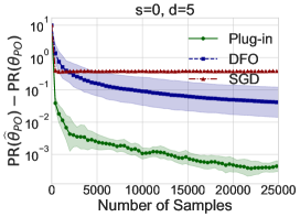
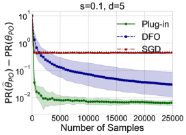
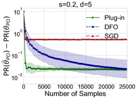
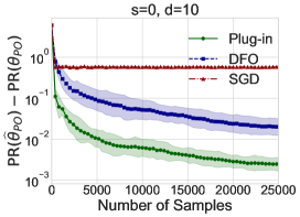
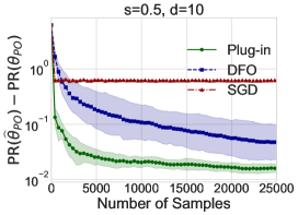
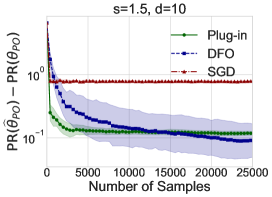
Figure 1: Excess risk versus $n$ for plug-in performative optimization, the DFO algorithm, and greedy SGD. Top: $d=5$. Bottom: $d=10$. We display the mean $\pm 1$ standard deviation, logarithmically scaled.

In Figure 1 we see that the excess risk of our algorithm converges rapidly to a value that reflects the degree of misspecification. When $s=0$ (left panel), the excess risk of our algorithm approaches zero as the number of samples increases, given that there is no misspecification. On the other hand, for $s>0$ (middle and right panels), the excess risk of our algorithm converges to a nonzero value, which is in accordance with our theoretical guarantee. Meanwhile, we see that the excess risk of DFO converges to zero at a slow rate, while SGD quickly converges to a highly suboptimal point.

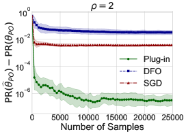
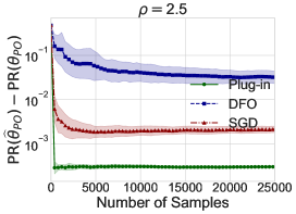
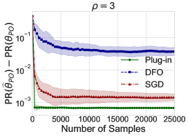
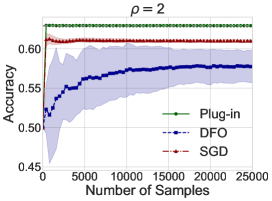
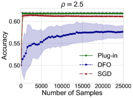
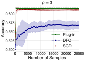
Figure 2: Excess risk (top) and accuracy (bottom) versus $n$ for plug-in performative optimization, the DFO algorithm, and greedy SGD, with $\tilde{\beta}=2$. We display the mean $\pm 1$ standard deviation, logarithmically scaled.

5.2 Strategic regression

We next consider strategic regression. We first generate $5000$ i.i.d. historical data points $(x_{i},y_{i})\in\mathbb{R}^{d_{x}}\times\{0,1\}$ where $x_{i}\sim{\mathcal{N}}(0,I_{d_{x}})$, and $y_{i}$ follows from a logistic model with a fixed parameter vector $\eta\sim{\mathrm{Unif}}(\mathcal{S}^{d_{x}-1})$. Denote the joint empirical distribution of $(x_{i},y_{i})$ by $\mathcal{D}_{0}$. The true distribution map is given by

$$(x,y)\sim\mathcal{D}(\theta)\Leftrightarrow(x_{0},y_{0})\sim\mathcal{D}_{0},y=y_{0},x=\operatorname*{arg\,max}_{x^{\prime}\in\mathbb{R}^{d_{x}}}\left(\theta^{\top}x^{\prime}-\frac{1}{2\tilde{\beta}}\|x^{\prime}-x_{0}\|_{\rho}^{\rho}\right)$$

for some $\rho>1$. We set $d_{x}=5$ vary $\tilde{\beta}\in\{1,2\}$. To construct a model for $\mathcal{D}(\cdot)$, we follow the procedure from Section 4.1, using the linear utility and quadratic cost, meaning $\rho=2$ results in correct specification. We choose $\ell(z;\theta)$ to be the logistic loss with a small ridge penalty, i.e.,

$$\ell(z,\theta)=\left[-y\cdot\log(\sigma(\theta^{T}x))-(1-y)\cdot\log(1-\sigma(\theta^{T}x))\right]+\lambda\|\theta\|^{2}_{2},$$

where $\sigma(s):=\exp\{s\}/(1+\exp\{s\})$ and $\lambda=0.001$. We choose $\Theta=\{\theta:\|\theta\|\leq 1\}$.

We consider both the well-specified scenario, $\rho=2$, and two misspecified scenarios, $\rho\in\{2.5,3\}$, and compare our method with DFO and greedy SGD. The results are shown in Figure 2 and Figure 3. As before, our algorithm exhibits rapid convergence to a point with zero excess risk when the model is well-specified (top left). Under misspecification (top middle and right), the algorithm still converges, albeit to a somewhat suboptimal point. In contrast, SGD converges to a suboptimal point with nonzero excess risk, while the excess risk of the DFO method decreases at a slow rate. In addition to the takeaways in terms of excess risk, we observe similar trends in terms of test accuracy (bottom panel).

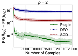
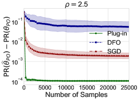
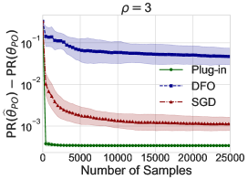
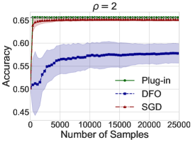
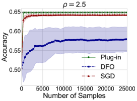
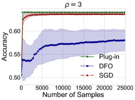
Figure 3: Excess risk (top) and accuracy (bottom) versus $n$ for plug-in performative optimization, the DFO algorithm, and greedy SGD, with $\tilde{\beta}=1$. We display the mean $\pm 1$ standard deviation, logarithmically scaled.

We run an analogous experiment on a real data set. We use the credit data set Yeh and Lien (2009), in particular the processed version from Ustun et al. (2019), available at this link. The data set contains $30,000$ samples of $d=17$ features and a $\{0,1\}$-valued outcome $y_{i}$ with $y_{i}=1$ denoting individual $i$ not defaulting on a credit card payment. The features include marital status, age, education level, and payment patterns. Like Ustun et al. Ustun et al. (2019), we assume the individuals can modify their records on education level and payment patterns (features $7$–$17$), but cannot change other records. We use $1500$ randomly drawn data points to form the base distribution $\mathcal{D}_{0}$; we assume the same true response model and use the same distribution atlas as before. We set $\tilde{\beta}=5$, $\Theta=\{\theta:\|\theta\|\leq 1\}$, and standardize the features so that each column is zero-mean and has unit variance. In Figure 4, we observe patterns similar to those in Figure 2 and 3, though the gap in accuracy between our method and SGD is smaller.

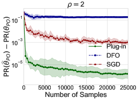
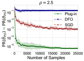
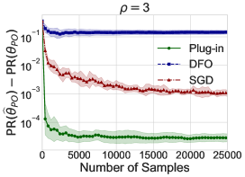
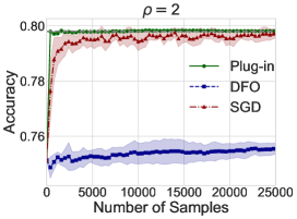
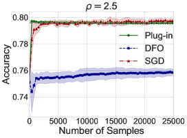
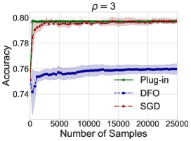
Figure 4: Excess risk (top) and accuracy (bottom) versus $n$ for plug-in performative optimization, the DFO algorithm, and greedy SGD, on the credit data set. We display the mean $\pm 1$ standard deviation, logarithmically scaled.

6 Conclusion

We have analyzed performative optimization with possibly misspecified models. Our results highlight the statistical gains of using models, however modeling can have consequences far beyond statistical efficiency. On the positive side, modeling can help interpretability and computational efficiency. On the negative side, however, using highly misspecified models can lead to unfairness, lack of validity, and poor downstream decisions. Going forward, it would be valuable to develop deeper understanding of such negative aspects of modeling. Overall, given that models are ubiquitous in practice, we believe they merit further study—especially under misspecification—and we have only scratched the surface of this agenda.

Appendix A Proofs

A.1 Notation and definitions

In the proofs we will sometimes use $c,c^{\prime}>0$ to denote universal constants and $C,C^{\prime}>0$ to denote constants that may depend on the parameters introduced in the assumptions. We allow the values of the constants to vary from place to place.

We say a random variable $x$ is subexponential with parameter $\nu$ (see e.g., the book by Vershynin [36]) if

$$\mathbb{P}\{|x|\geq t\}\leq 2\exp\left(-\frac{t}{\nu}\right)$$

for any $t\geq 0$. Unless specified, we do not assume $x$ has mean zero in general. Moreover, we say a vector $\mathbf{x}\in\mathbb{R}^{d}$ is subexponential with parameter $\nu$ if $\langle{u},\,\mathbf{x}\rangle$ is subexponential with parameter $\nu$ for any fixed direction ${u}\in\mathcal{S}^{d-1}$. Similarly, we say a random variable $x$ is subgaussian with parameter $\sigma$ if

$$\mathbb{P}\{|x|\geq t\}\leq 2\exp\left(-\frac{t^{2}}{\sigma^{2}}\right)$$

for any $t\geq 0$. Likewise, a vector $\mathbf{x}\in\mathbb{R}^{d}$ is subgaussian with parameter $\sigma$ if $\langle{u},\,\mathbf{x}\rangle$ is subgaussian with parameter $\sigma$ for any fixed direction ${u}\in\mathcal{S}^{d-1}$.

A.2 Proof of Theorem 2

Define the population-level counterpart of $\hat{\theta}_{\mathrm{PO}}$ as:

$$\theta^{*}=\operatorname*{arg\,min}_{\theta\in\Theta}\mathrm{PR}^{\beta^{*}}(\theta).$$

We can write

$$\mathrm{PR}(\hat{\theta}_{\mathrm{PO}})-\mathrm{PR}(\theta_{\mathrm{PO}})$$

$$\quad=(\mathrm{PR}(\hat{\theta}_{\mathrm{PO}})-\mathrm{PR}^{\beta^{*}}(\hat{\theta}_{\mathrm{PO}}))+(\mathrm{PR}^{\beta^{*}}(\hat{\theta}_{\mathrm{PO}})-\mathrm{PR}^{\hat{\beta}}(\hat{\theta}_{\mathrm{PO}}))+(\mathrm{PR}^{\hat{\beta}}(\hat{\theta}_{\mathrm{PO}})-\mathrm{PR}^{\hat{\beta}}(\theta^{*}))$$

$$\quad+(\mathrm{PR}^{\hat{\beta}}(\theta^{*})-\mathrm{PR}^{\beta^{*}}(\theta^{*}))+(\mathrm{PR}^{\beta^{*}}(\theta^{*})-\mathrm{PR}^{\beta^{*}}(\theta_{\mathrm{PO}}))+(\mathrm{PR}^{\beta^{*}}(\theta_{\mathrm{PO}})-\mathrm{PR}(\theta_{\mathrm{PO}})).$$

By the definition of $\hat{\theta}_{\mathrm{PO}}$, we know $\mathrm{PR}^{\hat{\beta}}(\hat{\theta})-\mathrm{PR}^{\hat{\beta}}(\theta^{*})\leq 0$. Similarly, by the definition of $\theta^{*}$, we know $\mathrm{PR}^{\beta^{*}}(\theta^{*})-\mathrm{PR}^{\beta^{*}}(\theta_{\mathrm{PO}})\leq 0$. Using these inequalities, we establish

$$\mathrm{PR}(\hat{\theta}_{\mathrm{PO}})-\mathrm{PR}(\theta_{\mathrm{PO}}) \leq(\mathrm{PR}(\hat{\theta}_{\mathrm{PO}})-\mathrm{PR}^{\beta^{*}}(\hat{\theta}_{\mathrm{PO}}))+(\mathrm{PR}^{\beta^{*}}(\hat{\theta}_{\mathrm{PO}})-\mathrm{PR}^{\hat{\beta}}(\hat{\theta}_{\mathrm{PO}}))$$

$$\quad+(\mathrm{PR}^{\hat{\beta}}(\theta^{*})-\mathrm{PR}^{\beta^{*}}(\theta^{*}))+(\mathrm{PR}^{\beta^{*}}(\theta_{\mathrm{PO}})-\mathrm{PR}(\theta_{\mathrm{PO}}))$$

$$\leq 2\sup_{\theta}|\mathrm{PR}(\theta)-\mathrm{PR}^{\beta^{*}}(\theta)|+2\sup_{\theta}|\mathrm{PR}^{\beta^{*}}(\theta)-\mathrm{PR}^{\hat{\beta}}(\theta)|$$

$$=2(\textup{{StatErr}}_{n}+\textup{{MisspecErr}}).$$

A.3 Proof of Corollary 1

We have

$$|\mathrm{PR}^{\beta^{*}}(\theta)-\mathrm{PR}(\theta)| =\left|\int\ell(z;\theta)(p_{\beta^{*}}(z;\theta)-p(z;\theta))dz\right|$$

$$\leq B_{\ell}\cdot\int|p_{\beta^{*}}(z;\theta)-p(z;\theta)|dz$$

$$=2B_{\ell}\cdot\mathrm{TV}(\mathcal{D}_{\beta^{*}}(\theta),\mathcal{D}(\theta)).$$

Therefore,

$$\texttt{MisspecErr}\leq 2B_{\ell}\sup_{\theta\in\Theta}\mathrm{TV}(\mathcal{D}_{\beta^{*}}(\theta),\mathcal{D}(\theta))\leq 2B_{\ell}\eta_{\mathrm{TV}}.$$

By a similar argument as above, $|\mathrm{PR}^{\beta^{*}}(\theta)-\mathrm{PR}^{\hat{\beta}}(\theta)|\leq 2B_{\ell}\mathrm{TV}(\mathcal{D}_{\beta^{*}}(\theta),\mathcal{D}_{\hat{\beta}}(\theta))$. Applying $\epsilon_{\mathrm{TV}}$-smoothness of the distribution atlas, we get

$$\texttt{StatErr}_{n}\leq 2B_{\ell}\sup_{\theta\in\Theta}\mathrm{TV}(\mathcal{D}_{\beta^{*}}(\theta),\mathcal{D}_{\hat{\beta}}(\theta))\leq 2B_{\ell}\epsilon_{\mathrm{TV}}\|\hat{\beta}-\beta^{*}\|\leq 2B_{\ell}\epsilon_{\mathrm{TV}}C_{n}.$$

Applying Theorem 2 completes the proof.

A.4 Proof of Corollary 2

Denote by $\Pi(\mathcal{D},\mathcal{D}^{\prime})$ a coupling between two distributions $\mathcal{D}$ and $\mathcal{D}^{\prime}$. We have

$$\left|\mathrm{PR}^{\beta^{*}}(\theta)-\mathrm{PR}(\theta)\right| =\left|\inf_{\Pi(\mathcal{D}_{\beta^{*}}(\theta),\mathcal{D}(\theta))}\mathbb{E}_{(z,z^{\prime})\sim\Pi(\mathcal{D}_{\beta^{*}}(\theta),\mathcal{D}(\theta))}[\ell(z;\theta)-\ell(z^{\prime};\theta)]\right|$$

$$\leq\inf_{\Pi(\mathcal{D}_{\beta^{*}}(\theta),\mathcal{D}(\theta))}\mathbb{E}_{(z,z^{\prime})\sim\Pi(\mathcal{D}_{\beta^{*}}(\theta),\mathcal{D}(\theta))}[|\ell(z;\theta)-\ell(z^{\prime};\theta)|]$$

$$\leq L\inf_{\Pi(\mathcal{D}_{\beta^{*}}(\theta),\mathcal{D}(\theta))}\mathbb{E}_{(z,z^{\prime})\sim\Pi(\mathcal{D}_{\beta^{*}}(\theta),\mathcal{D}(\theta))}[\|z-z^{\prime}\|]$$

$$=L\mathcal{W}(\mathcal{D}_{\beta^{*}}(\theta),\mathcal{D}(\theta)).$$

Therefore,

$$\texttt{MisspecErr}\leq L\sup_{\theta\in\Theta}\mathcal{W}(\mathcal{D}_{\beta^{*}}(\theta),\mathcal{D}(\theta))\leq L\cdot\eta_{W}.$$

By a similar argument, $|\mathrm{PR}^{\beta^{*}}(\theta)-\mathrm{PR}^{\hat{\beta}}(\theta)|\leq L\mathcal{W}(\mathcal{D}_{\beta^{*}}(\theta),\mathcal{D}_{\hat{\beta}}(\theta))$. Applying $\epsilon_{W}$-smoothness of the distribution atlas, we get

$$\texttt{StatErr}_{n}\leq L\sup_{\theta\in\Theta}\mathcal{W}(\mathcal{D}_{\beta^{*}}(\theta),\mathcal{D}_{\hat{\beta}}(\theta))\leq L\epsilon_{W}\|\hat{\beta}-\beta^{*}\|\leq L\cdot\epsilon_{W}\cdot C_{n}.$$

Applying Theorem 2 completes the proof.

A.5 Proof of Lemma 1

We first present a technical lemma that we will use in the proof. We defer its proof to the end of this subsection.

Lemma 2.

$$\langle\nabla{r}(\beta),\,\beta-\beta^{*}\rangle \geq\begin{dcases}\frac{\mu}{2}\|{\beta^{*}-\beta}\|^{2},&\|{\beta^{*}-\beta}\|\leq\frac{\mu}{\sigma_{r}},\\ \frac{\mu^{2}}{2\sigma_{r}}\|{\beta^{*}-\beta}\|,&\|\beta^{*}-\beta\|\geq\frac{\mu}{\sigma_{r}}.\end{dcases}$$ (3)

Let $B_{\beta}$ be the bound of the parameter set $\mathcal{B}$, i.e., $\|\beta\|\leq\mathcal{B}_{\beta}$ for any $\beta\in\mathcal{B}$. We will show Lemma 1 holds with some sufficiently large constants $C,C^{\prime}>0$ that depend polynomially on $(\log|1+B_{\beta}|,1/\mu,L_{r},B_{r},\sigma_{r})$.

Denote

$${r}_{n}(\beta):=\frac{1}{n}\sum_{i=1}^{n}{r}(\theta_{i},z_{i};\beta);~{}~{}~{}{r}(\beta):=\mathbb{E}_{\theta\sim\tilde{\mathcal{D}},z\sim\mathcal{D}(\theta)}[{r}(\theta,z;\beta)].$$

We begin by claiming the following result, which we will prove later. With probability over $1-\delta$

$$\sup_{\beta\in\mathcal{B}}\|\nabla_{\beta}{r}_{n}(\beta)-\nabla_{\beta}{r}(\beta)\| \leq C\sqrt{\log n}\sqrt{\frac{{d_{\beta}+\log(1/\delta)}}{n}}.$$ (4)

With this result at hand, it follows from Lemma 2 that

$$\min\Big{\{}\frac{\mu}{2}\|\hat{\beta}-\beta^{*}\|^{2},\frac{\mu^{2}}{2\sigma_{r}}\|\hat{\beta}-\beta^{*}\|\Big{\}} \leq\langle\nabla_{\beta}{r}(\hat{\beta}),\,\hat{\beta}-\beta^{*}\rangle=\langle\nabla_{\beta}{r}(\hat{\beta})-\nabla_{\beta}{r}_{n}(\hat{\beta}),\,\hat{\beta}-\beta^{*}\rangle$$

$$\leq\|\nabla_{\beta}{r}(\hat{\beta})-\nabla_{\beta}{r}_{n}(\hat{\beta})\|\|\hat{\beta}-\beta^{*}\|\leq C\sqrt{\log n}\sqrt{\frac{{d_{\beta}+\log(1/\delta)}}{n}}\|\hat{\beta}-\beta^{*}\|,$$ (5)

where the first equality is due to the fact that $\nabla_{\beta}{r}_{n}(\hat{\beta})=0$. Eliminating $\|\hat{\beta}-\beta^{*}\|$ in both the first and the last term of (5) yields

$$\frac{\mu^{2}}{2\sigma_{{r}}}\wedge\frac{\mu}{2}\|\hat{\beta}-\beta^{*}\|\leq C\sqrt{\log n}\sqrt{\frac{{d_{\beta}+\log(1/\delta)}}{n}}.$$

By the sample size Assumption in Lemma 1, we may assume $n$ is sufficiently large such that $\frac{\mu^{2}}{2\sigma_{{r}}}\geq C\sqrt{\log n}\sqrt{\frac{{d_{\beta}+\log(1/\delta)}}{n}}$ for some constant $C>0$. Therefore, we conclude that

$$\|\hat{\beta}-\beta^{*}\|\leq C\sqrt{\log n}\sqrt{\frac{{d_{\beta}+\log(1/\delta)}}{n}}.$$

Proof of Eq. (4).

Let $\{{u}_{1},{u}_{2},\ldots,{u}_{M}\}$ be a $1/2$-covering of $\mathcal{S}^{d_{\beta}-1}$ in the Euclidean norm such that $|M|\leq 5^{d_{\beta}}$. Define the random variables

$$\phi_{{u},\beta}:=\langle{u},\,\nabla_{\beta}{r}_{n}(\beta)-\nabla_{\beta}{r}(\beta)\rangle,~{}~{}\phi_{u}:=\sup_{\beta\in\mathcal{B}}\phi_{{u},\beta}.$$

It follows from a standard discretization argument (e.g., [37], Chap. 6) that

$$\sup_{\beta\in\mathcal{B}}\|\nabla_{\beta}{r}_{n}(\beta)-\nabla_{\beta}{r}(\beta)\|\leq 2\sup_{\beta\in\mathcal{B}}\sup_{i\in[M]}\phi_{{u}_{i},\beta}.$$ (6)

We make the following claim which will be proved at the end. With probability over $1-\delta$

$$\left\|\frac{1}{n}\sum_{i=1}^{n}\sup_{\beta\in\mathcal{B}}\nabla^{2}_{\beta}{r}(\theta_{i},z_{i};\beta)\right\|_{{\tiny{\mbox{op}}}}\leq cL_{r}+cL_{r}\sqrt{\frac{d_{\beta}+\log(1/\delta)}{n}}\leq cL_{r}.$$ (7)

for some constant $c>0$.

Let $\epsilon>0$ be some value we specify later. Construct an $\varepsilon$-covering net $\{\beta^{1},\ldots,\beta^{N}\}$ of $\mathcal{B}$ in $\|\cdot\|$. Then the covering number $|N|\leq(1+2B_{\beta}/\epsilon)^{d_{\beta}}$, and

$$\sup_{\beta\in\mathcal{B}}\sup_{i\in[M]}\phi_{{u}_{i},\beta} \leq\sup_{i\in[M]}\sup_{j\in[N]}\phi_{{u}_{i},\beta^{j}}+\sup_{i\in[M]}\sup_{\|\beta_{1}-\beta_{2}\|\leq\varepsilon}|\phi_{{u}_{i},\beta_{1}}-\phi_{{u}_{i},\beta_{2}}|$$

$$\leq\sup_{i\in[M]}\sup_{j\in[N]}\phi_{{u}_{i},\beta^{j}}+\sup_{i\in[M]}\sup_{\|\beta_{1}-\beta_{2}\|\leq\varepsilon}\frac{1}{n}\sum_{i=1}^{n}\sup_{\beta\in\mathcal{B}}{u}_{i}^{\top}\nabla^{2}_{\beta}{r}(\theta_{i},z_{i};\beta)(\beta_{1}-\beta_{2})$$

$$\leq\sup_{i\in[M]}\sup_{j\in[N]}\phi_{{u}_{i},\beta^{j}}+\sup_{i\in[M]}\sup_{\|\beta_{1}-\beta_{2}\|\leq\varepsilon}\|{u}_{i}\|\left\|\frac{1}{n}\sum_{i=1}^{n}\sup_{\beta\in\mathcal{B}}\nabla^{2}_{\beta}{r}(\theta_{i},z_{i};\beta)\right\|_{{\tiny{\mbox{op}}}}\|\beta_{1}-\beta_{2}\|$$

$$\leq\sup_{i\in[M]}\sup_{j\in[N]}\phi_{{u}_{i},\beta^{j}}+cL_{r}\varepsilon,$$ (8)

where the last inequality follows from the claim in  (7). Since $\langle{u},\,\nabla_{\beta}{r}(\theta_{i},z_{i};\beta)-\mathbb{E}[\nabla_{\beta}{r}(\theta_{i},z_{i};\beta)]\rangle$ is zero mean subexponential with parameter $B_{r}$ by condition (b) of Assumption 1, it follows from concentration of subexponential variables that

$$\mathbb{P}\{|\phi_{u_{i},\beta^{j}}|\geq t\}\leq 2\exp\left(-\frac{nt^{2}}{2B_{r}^{2}}\right)~{}~{}\text{ for any }|t|\leq B_{r}.$$

Applying a union bound over $i,j$, we establish

$$\mathbb{P}\left\{\max_{i\in[M],j\in[N]}|\phi_{u_{i},\beta^{j}}|\geq t\right\}\leq 2\exp\left(cd_{\beta}(\log(1+2B_{\beta}/\epsilon)+1)-\frac{nt^{2}}{2B_{r}^{2}}\right)~{}~{}\text{ for any }|t|\leq B_{r}.$$ (9)

Let $\epsilon=\sqrt{\frac{d_{\beta}+\log(1/\delta)}{n}}$ and

$$t=\frac{cB_{r}\sqrt{\log(1/\delta)+d_{\beta}(\log(1+2B_{\beta}/\epsilon)+1)}}{\sqrt{n}} \leq\frac{CB_{r}\sqrt{\log n(d_{\beta}+\log(1/\delta))}}{\sqrt{n}}\leq{B_{r}}$$

for some constant $c>0$, where the last inequality uses the sample size assumption of the lemma. Substituting the values of $\epsilon$ and $t$ into Equations (8), (9) and combining with Eq. (6), we obtain

$$\sup_{\beta\in\mathcal{B}}\|\nabla_{\beta}{r}_{n}(\beta)-\nabla_{\beta}{r}(\beta)\| \leq\frac{CB_{r}\sqrt{\log n(d_{\beta}+\log(1/\delta))}}{\sqrt{n}}+cL_{r}\sqrt{\frac{d_{\beta}+\log(1/\delta)}{n}}$$

$$\leq C^{\prime}\sqrt{\log n}\sqrt{\frac{{d_{\beta}+\log(1/\delta)}}{n}}$$

with probability over $1-\delta$ for some parameter-dependent constant $C^{\prime}$.

Proof of Eq. (7).

Similar to Eq. (6), from a standard discretization argument we have

$$\left\|\frac{1}{n}\sum_{i=1}^{n}\sup_{\beta\in\mathcal{B}}\nabla^{2}_{\beta}{r}(\theta_{i},z_{i};\beta)\right\|_{{\tiny{\mbox{op}}}}\leq 2\sup_{j\in[M]}\frac{1}{n}\sum_{i=1}^{n}\sup_{\beta\in\mathcal{B}}{u}_{j}^{\top}\nabla^{2}_{\beta}{r}(\theta_{i},z_{i};\beta){u}_{j}.$$

Since $\sup_{\beta\in\mathcal{B}}{u}_{j}^{\top}\nabla^{2}_{\beta}{r}(\theta_{i},z_{i};\beta){u}_{j}$ are subexponential variables by condition (c) in Assumption 1, we have from properties of subexponential variables and Bernstein’s inequality that

$$\quad\mathbb{P}\left\{{u}_{j}^{\top}\frac{1}{n}\sum_{i=1}^{n}\sup_{\beta\in\mathcal{B}}\nabla^{2}_{\beta}{r}(\theta_{i},z_{i};\beta){u}_{j}\geq cL_{r}+t\right\}$$

$$\leq\mathbb{P}\left\{{u}_{j}^{\top}\frac{1}{n}\sum_{i=1}^{n}\sup_{\beta\in\mathcal{B}}\nabla^{2}_{\beta}{r}(\theta_{i},z_{i};\beta){u}_{j}\geq\mathbb{E}[{u}_{j}^{\top}\sup_{\beta\in\mathcal{B}}\nabla^{2}_{\beta}{r}(\theta_{i},z_{i};\beta){u}_{j}]+t\right\}$$

$$\leq\exp\left(-c\min\{\frac{nt}{L_{r}},\frac{nt^{2}}{L_{r}^{2}}\}\right).$$

Applying a union bound over $j\in[M]$ and setting $t=cL_{r}\sqrt{\frac{d_{\beta}+\log(1/\delta)}{n}}<cL_{r}$, we establish

$${u}_{j}^{\top}\frac{1}{n}\sum_{i=1}^{n}\sup_{\beta\in\mathcal{B}}\nabla^{2}_{\beta}{r}(\theta_{i},z_{i};\beta){u}_{j}\leq cL_{r}+cL_{r}\sqrt{\frac{d_{\beta}+\log(1/\delta)}{n}}\leq cL_{r}$$

for some $c>0$ with probability over $1-\delta$.

Proof of Lemma 2.

For any $\|{\beta^{*}-\beta}\|\leq\frac{\mu}{\sigma_{r}}$, by a Taylor expansion of $\nabla{r}(\beta)$ at $\beta^{*}$ and Ass. 1(a), we have

$$\langle\nabla{r}(\beta),\,\beta-\beta^{*}\rangle=\langle\nabla{r}(\beta)-\nabla{r}(\beta^{*}),\,\beta-\beta^{*}\rangle\geq{\mu}\|\beta-\beta^{*}\|^{2}-\frac{\sigma_{r}}{2}\|\beta^{*}-\beta\|^{3}\geq\frac{\mu}{2}\|\beta^{*}-\beta\|^{2}.$$

This gives the second part of Lemma 2. When $\|{\beta^{*}-\beta}\|\geq\frac{\mu}{\sigma_{r}}$, write $\beta=\beta^{*}+t{u}$, where ${u}=(\beta-\beta^{*})/\|\beta-\beta^{*}\|$. For a fixed direction ${u}$, define $\beta(t):=\beta^{*}+t{u}$ and

$$f({u},t):=\Big{\langle}{\nabla{r}(\beta(t))},\frac{\beta(t)-\beta^{*}}{\|\beta(t)-\beta^{*}\|}\Big{\rangle}=\langle{u},\,\nabla{r}(\beta(t))\rangle.$$

Then for $t\geq 0$, using Ass. 1(a) again we obtain

$$\partial_{t}f({u},t)=\langle{u},\,\nabla^{2}{r}(\beta(t)){u}\rangle\geq 0$$

Therefore $f({u},t)$ is increasing in $t$ and for any $\|\beta-\beta^{*}\|\geq\frac{\mu}{\sigma_{{r}}}$

$$\Big{\langle}{\nabla{r}(\beta)},{\frac{\beta-\beta^{*}}{\|\beta-\beta^{*}\|}}\Big{\rangle} \geq\Big{\langle}\nabla{r}\Big{(}\beta\Big{(}\frac{\mu}{\sigma_{r}}\Big{)}\Big{)},\frac{\beta\Big{(}\frac{\mu}{\sigma_{r}}\Big{)}-\beta^{*}}{\|\beta\Big{(}\frac{\mu}{\sigma_{r}}\Big{)}-\beta^{*}\|}\Big{\rangle}$$

$$\geq\frac{\mu}{2}\|\beta\Big{(}\frac{\mu}{\sigma_{r}}\Big{)}-\beta^{*}\|=\frac{\mu^{2}}{2\sigma_{r}}.$$

This gives the second part of Lemma 2. ∎

A.6 Proof of Theorem 3

The first statement follows directly by putting together Corollary 1 and Lemma 1. Similarly, the second statement follows by putting together Corollary 2 and Lemma 1.

A.7 Proof of Claim 1

Fix $x$ and $\theta$. We will use the shorthand notation $g_{\beta}(x,\theta)\equiv x_{\beta}$. First, we show that $\|x_{\beta}-x_{\beta^{\prime}}\|_{2}\leq\frac{B_{u}}{1-\beta_{\max}L_{u}}|\beta-\beta^{\prime}|$. To see this, notice that the optimality condition of the best-response equation is equal to:

$$\beta\cdot\nabla u_{\theta}(x_{\beta})-x_{\beta}=-x.$$

Since $\beta\nabla u_{\theta}(x_{\beta})-x_{\beta}=\beta^{\prime}\nabla u_{\theta}(x_{\beta^{\prime}})-x_{\beta^{\prime}}=-x$, we know

$$\left\|\beta\nabla u_{\theta}(x_{\beta})-\beta^{\prime}\nabla u_{\theta}(x_{\beta^{\prime}})\right\|=\|x_{\beta}-x_{\beta^{\prime}}\|.$$

We also know

$$\left\|\beta\nabla u_{\theta}(x_{\beta})-\beta^{\prime}\nabla u_{\theta}(x_{\beta^{\prime}})\right\| =\left\|\beta\nabla u_{\theta}(x_{\beta})-\beta\nabla u_{\theta}(x_{\beta^{\prime}})+\beta\nabla u_{\theta}(x_{\beta^{\prime}})-\beta^{\prime}\nabla u_{\theta}(x_{\beta^{\prime}})\right\|$$

$$\leq\beta L_{u}\|x_{\beta}-x_{\beta^{\prime}}\|+B_{u}\left|\beta-\beta^{\prime}\right|.$$

Therefore,

$$\|x_{\beta}-x_{\beta^{\prime}}\|\leq\beta L_{u}\|x_{\beta}-x_{\beta^{\prime}}\|+B_{u}\left|\beta-\beta^{\prime}\right|.$$

Rearranging the terms, we get

$$\|x_{\beta}-x_{\beta^{\prime}}\|\leq\frac{B_{u}}{1-\beta L_{u}}|\beta-\beta^{\prime}|.$$

By the definition of Wasserstein distance, this condition directly implies

$$\mathcal{W}(\mathcal{D}_{\beta}(\theta),\mathcal{D}_{\beta^{\prime}}(\theta))\leq\frac{B_{u}}{1-\beta_{\max}L_{u}}|\beta-\beta^{\prime}|,$$

which is the definition of $\frac{B_{u}}{1-\beta_{\max}L_{u}}$-smoothness.

A.8 Proof of Claim 2

The claim follows by Lemma 1 after verifying the conditions required in Assumption 1. We have $r(\theta,x;\beta)=\|x-\beta\nabla u_{\theta}(x)\|^{2}$, so $\nabla r(\theta,x;\beta)=-2(x^{\top}\nabla u_{\theta}(x)-\beta\|\nabla u_{\theta}(x)\|^{2})$ and $\nabla^{2}r(\theta,x;\beta)=2\|\nabla u_{\theta}(x)\|^{2}$. Conditions (b) and (c) of Assumption 1 are thus satisfied by $\tilde{x}$ and $\nabla u_{\tilde{\theta}}(\tilde{x})$ being subgaussian since products of subgaussians are subexponential. Condition (a) is satisfied by the fact that $r(\beta)=\mathbb{E}[\|\tilde{x}-\beta\nabla u_{\tilde{\theta}}(\tilde{x})\|^{2}]$ is a quadratic in $\beta$ when $\mathbb{E}[\|\nabla u_{\tilde{\theta}}(\tilde{x})\|^{2}]>0$.

A.9 Proof of Claim 3

Fix $\theta,\beta,\beta^{\prime}$, and without loss of generality let $\beta>\beta^{\prime}$. We show that $\mathrm{TV}(\mathcal{D}_{\beta}(\theta),\mathcal{D}_{\beta^{\prime}}(\theta))\leq\phi_{u}$. The distributions $\mathcal{D}_{\beta}(\theta)$ and $\mathcal{D}_{\beta^{\prime}}(\theta)$ are equal to each other and to $\mathcal{D}_{0}$ for all $\{x:x^{\top}\theta\in(-\infty,T-\beta)\cup(T,\infty)\}$. Moreover, under both $\mathcal{D}_{\beta}(\theta)$ and $\mathcal{D}_{\beta^{\prime}}(\theta)$, there is no mass for $\{x:x^{\top}\theta\in(T-\beta^{\prime},T)\}$. The distributions thus only differ for $\{x:x^{\top}\theta\in[T-\beta,T-\beta^{\prime}]\cup\{T\}\}$. Since the density of $x^{\top}\theta$ is bounded by $\phi_{u}$, the measure of such vectors $x$ is at most $\phi_{u}|\beta-\beta^{\prime}|$.

A.10 Proof of Claim 4

By Hoeffding’s inequality, with probability $1-\delta$ it holds that

$$\left|\frac{1}{n}\sum_{i=1}^{n}\mathbf{1}\{x_{i}^{\top}\theta_{i}\in(T\pm\epsilon)\}-\mathbb{P}\{\tilde{x}^{\top}\tilde{\theta}\in(T\pm\epsilon)\}\right|\leq\sqrt{\frac{\log(2/\delta)}{2n}}.$$

Let $\Delta=\sqrt{\frac{\log(2/\delta)}{2n}}$. Next we argue that $|\hat{\beta}-\beta^{*}|\leq\frac{\Delta}{\phi_{l}}$ by contradiction. Suppose $|\hat{\beta}-\beta^{*}|>\frac{\Delta}{\phi_{l}}$. Then,

$$\left|\frac{1}{n}\sum_{i=1}^{n}\mathbf{1}\{x_{i}^{\top}\theta_{i}\in(T\pm\epsilon)\}-\mathbb{P}\{\tilde{x}^{\top}\tilde{\theta}\in(T\pm\epsilon)\}\right| =\left|\mathbb{P}\{x_{0}^{\top}\tilde{\theta}\in[T-\hat{\beta},T]-\mathbb{P}\{x_{0}^{\top}\tilde{\theta}\in[T-\beta^{*},T]\}\right|$$

$$>\phi_{l}\frac{\Delta}{\phi_{l}}$$

$$=\Delta,$$

which contradicts Hoeffding’s inequality. Therefore, we conclude that $|\hat{\beta}-\beta^{*}|\leq\frac{\Delta}{\phi_{l}}$.

A.11 Proof of Claim 5

By the definition of Wasserstein distance, we have

$$\mathcal{W}(\mathcal{D}_{\mathcal{M}_{1}}(\theta),\mathcal{D}_{\mathcal{M}_{2}}(\theta))=\mathcal{W}(\mathcal{M}_{1}\theta+z_{0},\mathcal{M}_{2}\theta+z_{0})=\|\mathcal{M}_{1}\theta-\mathcal{M}_{2}\theta\|\leq B_{\theta}\left\|\mathcal{M}_{1}-\mathcal{M}_{2}\right\|_{{\tiny{\mbox{op}}}}$$

for any $\mathcal{M}_{1},\mathcal{M}_{2}$. Therefore, the distribution atlas $\{\mathcal{D}_{\mathcal{M}}\}_{\mathcal{M}}$ is $\epsilon_{W}$-smooth with parameter $B_{\theta}$.

A.12 Proof of Claim 6

Let $\nu_{\theta}$ be the subgaussian parameter of $\tilde{\mathcal{D}}$. We prove that there exists $C,C^{\prime}$ depending polynomially on $(1/\kappa_{\min},\kappa_{\max},\nu_{\theta},L_{\theta z},B)$ such that Claim 6 holds. By definition, we have

$$\widehat{\mathcal{M}}^{\top} =\left(\frac{1}{n}\sum_{i=1}^{n}\theta_{i}\theta_{i}^{\top}\right)^{-1}\Big{(}\frac{1}{n}\sum_{i=1}^{n}\theta_{i}z_{i}^{\top}\Big{)},$$

$$\mathcal{M}^{*\top} =\mathbb{E}[\tilde{\theta}\tilde{\theta}^{\top}]^{-1}\mathbb{E}[\tilde{\theta}\tilde{z}^{\top}].$$

We state the following results, which we will prove later:

$$\left\|\left(\frac{1}{n}\sum_{i=1}^{n}\theta_{i}\theta_{i}^{\top}\right)^{-1}-\mathbb{E}[\theta_{i}\theta_{i}^{\top}]^{-1}\right\|_{{\tiny{\mbox{op}}}} \leq\frac{c\nu_{\theta}^{2}}{\kappa_{\min}^{2}}\sqrt{\frac{d_{\theta}+\log(1/\delta)}{n}}\leq C;$$ (10)

$$\left\|\frac{1}{n}\sum_{i=1}^{n}\theta_{i}z_{i}^{\top}-\mathbb{E}[\theta_{i}z_{i}^{\top}]\right\|_{{\tiny{\mbox{op}}}} \leq cL_{\theta,z}\sqrt{\frac{d_{\theta}+d_{z}+\log(1/\delta)}{n}}.$$ (11)

Combining Equations (10), (11) with the assumptions of the claim, we establish

$$\left\|\widehat{\mathcal{M}}-\mathcal{M}^{*}\right\|_{{\tiny{\mbox{op}}}} =\left\|\left(\frac{1}{n}\sum_{i=1}^{n}\theta_{i}\theta_{i}^{\top}\right)^{-1}\Big{(}\frac{1}{n}\sum_{i=1}^{n}\theta_{i}z_{i}^{\top}\Big{)}-\mathbb{E}[\theta_{i}\theta_{i}^{\top}]^{-1}\mathbb{E}[\theta_{i}z_{i}^{\top}]\right\|_{{\tiny{\mbox{op}}}}$$

$$\leq\left\|\left(\frac{1}{n}\sum_{i=1}^{n}\theta_{i}\theta_{i}^{\top}\right)^{-1}-\mathbb{E}[\theta_{i}\theta_{i}^{\top}]^{-1}\right\|_{{\tiny{\mbox{op}}}}\left\|\frac{1}{n}\sum_{i=1}^{n}\theta_{i}z_{i}^{\top}\right\|_{{\tiny{\mbox{op}}}}$$

$$\quad+\left\|\mathbb{E}[\theta_{i}\theta_{i}^{\top}]^{-1}\right\|_{{\tiny{\mbox{op}}}}\left\|\frac{1}{n}\sum_{i=1}^{n}\theta_{i}z_{i}^{\top}-\mathbb{E}[\theta_{i}z_{i}^{\top}]\right\|_{{\tiny{\mbox{op}}}}$$

$$\leq C^{\prime}\sqrt{\frac{d_{\theta}+d_{z}+\log(1/\delta)}{n}}.$$

for some $C^{\prime}>0$ that depends on problem-specific parameters.

Proof of Eq. (10).

Under the conditions of the claim, we establish from concentration inequalities for subgaussian vectors (see, e.g., Theorem 6.5 in Wainwright [37]) that with probability at least $1-\delta$,

$$\frac{\kappa_{\min}}{2} \leq\kappa_{\min}-c\nu_{\theta}^{2}\sqrt{\frac{d_{\theta}+\log(1/\delta)}{n}}\leq\sigma_{\min}\left(\frac{1}{n}\sum_{i=1}^{n}\theta_{i}\theta_{i}^{\top}\right),$$

$$\leq\sigma_{\max}\left(\frac{1}{n}\sum_{i=1}^{n}\theta_{i}\theta_{i}^{\top}\right)\leq\kappa_{\max}+c\nu_{\theta}^{2}\sqrt{\frac{d_{\theta}+\log(1/\delta)}{n}}\leq\frac{3}{2}\kappa_{\max},$$

where the last line follows from the sample-size assumption. In addition, we also have from Wainwright [37] that

$$\left\|\frac{1}{n}\sum_{i=1}^{n}\theta_{i}\theta_{i}^{\top}-\mathbb{E}[\theta_{i}\theta_{i}^{\top}]\right\|_{{\tiny{\mbox{op}}}}\leq c\nu_{\theta}^{2}\sqrt{\frac{d_{\theta}+\log(1/\delta)}{n}}.$$

Therefore, it follows from Woodbury’s matrix identity and the last two displays that

$$\left\|\left(\frac{1}{n}\sum_{i=1}^{n}\theta_{i}\theta_{i}^{\top}\right)^{-1}-\mathbb{E}[\theta_{i}\theta_{i}^{\top}]^{-1}\right\|_{{\tiny{\mbox{op}}}} =\left\|\left(\frac{1}{n}\sum_{i=1}^{n}\theta_{i}\theta_{i}^{\top}\right)^{-1}\left(\left(\frac{1}{n}\sum_{i=1}^{n}\theta_{i}\theta_{i}^{\top}\right)-\mathbb{E}[\theta_{i}\theta_{i}^{\top}]\right)(\mathbb{E}[\theta_{i}\theta_{i}^{\top}])^{-1}\right\|_{{\tiny{\mbox{op}}}}$$

$$\leq\left\|\left(\frac{1}{n}\sum_{i=1}^{n}\theta_{i}\theta_{i}^{\top}\right)^{-1}\right\|_{{\tiny{\mbox{op}}}}\left\|\frac{1}{n}\sum_{i=1}^{n}\theta_{i}\theta_{i}^{\top}-\mathbb{E}[\theta_{i}\theta_{i}^{\top}]\right\|_{{\tiny{\mbox{op}}}}\left\|(\mathbb{E}[\theta_{i}\theta_{i}^{\top}])^{-1}\right\|_{{\tiny{\mbox{op}}}}$$

$$\leq\frac{c\nu_{\theta}^{2}}{\kappa_{\min}^{2}}\sqrt{\frac{d_{\theta}+\log(1/\delta)}{n}}.$$

The second inequality follows from the assumption on sample size.

Proof of Eq. (11).

Let $\{{u}_{1},\ldots,{u}_{M}\}$ be a $1/4$-covering of $\mathcal{S}^{d_{\theta}-1}$ in the Euclidean norm with $|M|\leq 9^{d_{\theta}}$, and $\{{v}_{1},\ldots,{v}_{N}\}$ to be a $1/4$-covering of $\mathcal{S}^{d_{z}-1}$ with $|N|\leq 9^{d_{z}}$. Then by a standard discretization argument, we have

$$\left\|\frac{1}{n}\sum_{i=1}^{n}\theta_{i}z_{i}^{\top}-\mathbb{E}[\theta_{i}z_{i}]\right\|_{{\tiny{\mbox{op}}}}\leq 2\sup_{k\in[M],l\in[N]}\frac{1}{n}\sum_{i=1}^{n}{u}_{k}^{\top}\theta_{i}z_{i}^{\top}{v}_{l}-\mathbb{E}[{u}_{k}^{\top}\theta_{i}z_{i}^{\top}{v}_{l}].$$

Since ${u}_{k}^{\top}\theta_{i}z_{i}^{\top}{v}_{l}-\mathbb{E}[{u}_{k}^{\top}\theta_{i}z_{i}^{\top}{v}_{l}]$ are zero-mean subexponential variables by assumption, it follows that

$$\mathbb{P}\left\{\left|\frac{1}{n}\sum_{i=1}^{n}{u}_{k}^{\top}\theta_{i}z_{i}^{\top}{v}_{l}-\mathbb{E}[{u}_{k}^{\top}\theta_{i}z_{i}^{\top}{v}_{l}]\right|\geq t\right\}\leq 2\exp\left(-c\min\left\{\frac{nt^{2}}{L_{\theta z}^{2}},\frac{nt}{L_{\theta z}}\right\}\right).$$

Applying a union bound over $M,N$ and setting $t=cL_{\theta z}\sqrt{\frac{d_{\theta}+d_{z}+\log(1/\delta)}{n}}<cL_{\theta z}$ with some sufficiently large constant $c>0$ yields

$$\quad\mathbb{P}\left\{\left\|\frac{1}{n}\sum_{i=1}^{n}{u}_{k}^{\top}\theta_{i}z_{i}^{\top}{v}_{l}-\mathbb{E}[{u}_{k}^{\top}\theta_{i}z_{i}^{\top}{v}_{l}]\right\|_{{\tiny{\mbox{op}}}}\geq t\right\}$$

$$\leq\mathbb{P}\left\{\sup_{k,l}\left|\frac{1}{n}\sum_{i=1}^{n}{u}_{k}^{\top}\theta_{i}z_{i}^{\top}{v}_{l}-\mathbb{E}[{u}_{k}^{\top}\theta_{i}z_{i}^{\top}{v}_{l}]\right|\geq t\right\}$$

$$\leq 2\exp\left((d_{\theta}+d_{z})\log 9-c\min\left\{\frac{nt^{2}}{L_{\theta z}^{2}},\frac{nt}{L_{\theta z}}\right\}\right)\leq\delta,$$

which gives Eq. (11).

Appendix B Experimental details

We provide implementation details for the two considered baselines.

Derivative-free optimization [8].

Starting from $\theta_{0}=\mathbf{1}_{d}/\sqrt{d}$, we run the updates

$$\theta_{t+1}=\mathrm{Proj}_{\|\cdot\|\leq 1}(\theta_{t}-\eta_{t}\widehat{\mathbb{E}}[{u}\mathrm{PR}(\theta_{t}+\delta{u})d/\delta])$$

for $t\geq 0$, where the step size $\eta_{t}=c_{0}/(t+1)$, ${u}$ is uniformly distributed on $\mathcal{S}^{d-1}$, and $\widehat{\mathbb{E}}[{u}\mathrm{PR}(\theta_{t}+\delta{u})d/\delta]$ denotes the unbiased sample estimation of $\mathbb{E}[{u}\mathrm{PR}(\theta_{t}+\delta{u})d/\delta]$ using $m$ i.i.d. pairs of $({u},z)\sim\mathrm{Unif}(\mathcal{S}^{d-1})\times\mathcal{D}(\theta_{t}+\delta{u})$. The projection $\mathrm{Proj}_{\|\cdot\|\leq 1}(x)$ denotes the projection of $x\in\mathbb{R}^{d}$ onto the ball $\{v\in\mathbb{R}^{d}:\|v\|\leq 1\}$ in Euclidean norm. We choose the step size parameter $c_{0}\in[10^{-4},10^{-1}]$, the batch size $m$ in $[1,500]$, and $\delta\in[0.1,100]$ via grid search.

Greedy stochastic gradient descent [23].

Starting from $\theta_{0}=\mathrm{1}_{d}/\sqrt{d}$, we run the updates

$$\theta_{t+1}=\mathrm{Proj}_{\|\cdot\|\leq 1}(\theta_{t}-\eta_{t}\nabla_{\theta}\ell(z_{t};\theta_{t}))$$

with step size $\eta_{t}=c_{0}/(t+1)$ and $z_{t}\sim\mathcal{D}(\theta_{t})$. The step size parameter $c_{0}\in[10^{-4},10]$ is selected via grid search. The greedy SGD algorithm neglects the implicit dependence of $z$ on $\theta$ due to performativity, and therefore typically converges to points suboptimal in terms of performative risk.

References

- Brown et al. [2022] Gavin Brown, Shlomi Hod, and Iden Kalemaj. Performative prediction in a stateful world. In International Conference on Artificial Intelligence and Statistics, pages 6045–6061. PMLR, 2022.
- Buja et al. [2019a] Andreas Buja, Lawrence Brown, Richard Berk, Edward George, Emil Pitkin, Mikhail Traskin, Kai Zhang, and Linda Zhao. Models as approximations I: Consequences illustrated with linear regression. Statistical Science, 34(4):523–544, 2019a.
- Buja et al. [2019b] Andreas Buja, Lawrence Brown, Arun Kumar Kuchibhotla, Richard Berk, Edward George, and Linda Zhao. Models as approximations II: A model-free theory of parametric regression. Statistical Science, 34(4):545–565, 2019b.
- Chen et al. [2020] Yiling Chen, Yang Liu, and Chara Podimata. Learning strategy-aware linear classifiers. Advances in Neural Information Processing Systems, 33:15265–15276, 2020.
- Dean et al. [2022] Sarah Dean, Mihaela Curmei, Lillian J Ratliff, Jamie Morgenstern, and Maryam Fazel. Multi-learner risk reduction under endogenous participation dynamics. arXiv preprint arXiv:2206.02667, 2022.
- Dong et al. [2018] Jinshuo Dong, Aaron Roth, Zachary Schutzman, Bo Waggoner, and Zhiwei Steven Wu. Strategic classification from revealed preferences. In Proceedings of the 2018 ACM Conference on Economics and Computation, pages 55–70, 2018.
- Drusvyatskiy and Xiao [2022] Dmitriy Drusvyatskiy and Lin Xiao. Stochastic optimization with decision-dependent distributions. Mathematics of Operations Research, 2022.
- Flaxman et al. [2004] Abraham D. Flaxman, Adam Tauman Kalai, and H. B. McMahan. Online convex optimization in the bandit setting: gradient descent without a gradient. In ACM-SIAM Symposium on Discrete Algorithms, 2004.
- Geer [2000] Sara A Geer. Empirical Processes in M-estimation, volume 6. Cambridge university press, 2000.
- Ghalme et al. [2021] Ganesh Ghalme, Vineet Nair, Itay Eilat, Inbal Talgam-Cohen, and Nir Rosenfeld. Strategic classification in the dark. In International Conference on Machine Learning, pages 3672–3681. PMLR, 2021.
- Hardt et al. [2016] Moritz Hardt, Nimrod Megiddo, Christos Papadimitriou, and Mary Wootters. Strategic classification. In Proceedings of the 2016 ACM conference on innovations in theoretical computer science, pages 111–122, 2016.
- Izzo et al. [2021] Zachary Izzo, Lexing Ying, and James Zou. How to learn when data reacts to your model: performative gradient descent. In International Conference on Machine Learning, pages 4641–4650. PMLR, 2021.
- Izzo et al. [2022] Zachary Izzo, James Zou, and Lexing Ying. How to learn when data gradually reacts to your model. In International Conference on Artificial Intelligence and Statistics, pages 3998–4035. PMLR, 2022.
- Jagadeesan et al. [2021] Meena Jagadeesan, Celestine Mendler-Dünner, and Moritz Hardt. Alternative microfoundations for strategic classification. In International Conference on Machine Learning, pages 4687–4697. PMLR, 2021.
- Jagadeesan et al. [2022] Meena Jagadeesan, Tijana Zrnic, and Celestine Mendler-Dünner. Regret minimization with performative feedback. In International Conference on Machine Learning, pages 9760–9785. PMLR, 2022.
- Kennedy [2022] Edward H Kennedy. Semiparametric doubly robust targeted double machine learning: a review. arXiv preprint arXiv:2203.06469, 2022.
- Kim and Perdomo [2022] Michael P Kim and Juan C Perdomo. Making decisions under outcome performativity. arXiv preprint arXiv:2210.01745, 2022.
- Kleinberg and Raghavan [2020] Jon Kleinberg and Manish Raghavan. How do classifiers induce agents to invest effort strategically? ACM Transactions on Economics and Computation (TEAC), 8(4):1–23, 2020.
- Kleinberg et al. [2008] Robert Kleinberg, Aleksandrs Slivkins, and Eli Upfal. Multi-armed bandits in metric spaces. In Proceedings of the fortieth annual ACM symposium on Theory of computing, pages 681–690, 2008.
- Levanon and Rosenfeld [2021] Sagi Levanon and Nir Rosenfeld. Strategic classification made practical. In International Conference on Machine Learning, pages 6243–6253. PMLR, 2021.
- Li and Wai [2022] Qiang Li and Hoi-To Wai. State dependent performative prediction with stochastic approximation. In International Conference on Artificial Intelligence and Statistics, pages 3164–3186. PMLR, 2022.
- Maheshwari et al. [2022] Chinmay Maheshwari, Chih-Yuan Chiu, Eric Mazumdar, Shankar Sastry, and Lillian Ratliff. Zeroth-order methods for convex-concave min-max problems: Applications to decision-dependent risk minimization. In International Conference on Artificial Intelligence and Statistics, pages 6702–6734. PMLR, 2022.
- Mendler-Dünner et al. [2020] Celestine Mendler-Dünner, Juan Perdomo, Tijana Zrnic, and Moritz Hardt. Stochastic optimization for performative prediction. Advances in Neural Information Processing Systems, 33:4929–4939, 2020.
- Mendler-Dünner et al. [2022] Celestine Mendler-Dünner, Frances Ding, and Yixin Wang. Anticipating performativity by predicting from predictions. Advances in Neural Information Processing Systems, 35:31171–31185, 2022.
- Miller et al. [2021] John P Miller, Juan C Perdomo, and Tijana Zrnic. Outside the echo chamber: Optimizing the performative risk. In International Conference on Machine Learning, pages 7710–7720. PMLR, 2021.
- Mou et al. [2019] Wenlong Mou, Nhat Ho, Martin J Wainwright, Peter Bartlett, and Michael I Jordan. A diffusion process perspective on posterior contraction rates for parameters. arXiv preprint arXiv:1909.00966, 2019.
- Narang et al. [2022] Adhyyan Narang, Evan Faulkner, Dmitriy Drusvyatskiy, Maryam Fazel, and Lillian Ratliff. Learning in stochastic monotone games with decision-dependent data. In International Conference on Artificial Intelligence and Statistics, pages 5891–5912. PMLR, 2022.
- Perdomo et al. [2020] Juan Perdomo, Tijana Zrnic, Celestine Mendler-Dünner, and Moritz Hardt. Performative prediction. In International Conference on Machine Learning, pages 7599–7609. PMLR, 2020.
- Piliouras and Yu [2022] Georgios Piliouras and Fang-Yi Yu. Multi-agent performative prediction: From global stability and optimality to chaos. arXiv preprint arXiv:2201.10483, 2022.
- Qiang et al. [2022] LI Qiang, Chung-Yiu Yau, and Hoi To Wai. Multi-agent performative prediction with greedy deployment and consensus seeking agents. In Advances in Neural Information Processing Systems, 2022.
- Ray et al. [2022] Mitas Ray, Lillian J Ratliff, Dmitriy Drusvyatskiy, and Maryam Fazel. Decision-dependent risk minimization in geometrically decaying dynamic environments. In Proceedings of the AAAI Conference on Artificial Intelligence, volume 36, pages 8081–8088, 2022.
- Spence [1978] Michael Spence. Job market signaling. In Uncertainty in economics, pages 281–306. Elsevier, 1978.
- Tsiatis [2007] A. Tsiatis. Semiparametric Theory and Missing Data. New York: Springer, 2007.
- Ustun et al. [2019] Berk Ustun, Alexander Spangher, and Yang Liu. Actionable recourse in linear classification. In Proceedings of the conference on fairness, accountability, and transparency, pages 10–19, 2019.
- Van der Vaart [2000] Aad W Van der Vaart. Asymptotic statistics, volume 3. Cambridge university press, 2000.
- Vershynin [2018] Roman Vershynin. High-dimensional probability: An introduction with applications in data science, volume 47. Cambridge university press, 2018.
- Wainwright [2019] M. J. Wainwright. High-dimensional statistics: A non-asymptotic viewpoint, volume 48. Cambridge University Press, 2019.
- White [1980] H. White. A heteroskedasticity-consistent covariance matrix estimator and a direct test for heteroskedasticity. Econometrica, 48:817–838, 1980.
- White [1982] Halbert White. Maximum likelihood estimation of misspecified models. Econometrica, 50(1):1–25, 1982. ISSN 00129682, 14680262. URL http://www.jstor.org/stable/1912526.
- Wooldridge [2003] Michael Wooldridge. Reasoning about rational agents. MIT press, 2003.
- Yeh and Lien [2009] I-Cheng Yeh and Che-hui Lien. The comparisons of data mining techniques for the predictive accuracy of probability of default of credit card clients. Expert systems with applications, 36(2):2473–2480, 2009.
- Zrnic et al. [2021] Tijana Zrnic, Eric Mazumdar, Shankar Sastry, and Michael Jordan. Who leads and who follows in strategic classification? Advances in Neural Information Processing Systems, 34:15257–15269, 2021.