Towards Accurate Data-free Quantization for Diffusion Models

Abstract

In this paper, we propose an accurate data-free post-training quantization framework of diffusion models (ADP-DM) for efficient image generation. Conventional data-free quantization methods learn shared quantization functions for tensor discretization regardless of the generation timesteps, while the activation distribution differs significantly across various timesteps. The calibration images are acquired in random timesteps which fail to provide sufficient information for generalizable quantization function learning. Both issues cause sizable quantization errors with obvious image generation performance degradation. On the contrary, we design group-wise quantization functions for activation discretization in different timesteps and sample the optimal timestep for informative calibration image generation, so that our quantized diffusion model can reduce the discretization errors with negligible computational overhead. Specifically, we partition the timesteps according to the importance weights of quantization functions in different groups, which are optimized by differentiable search algorithms. We also select the optimal timestep for calibration image generation by structural risk minimizing principle in order to enhance the generalization ability in the deployment of quantized diffusion model. Extensive experimental results show that our method outperforms the state-of-the-art post-training quantization of diffusion model by a sizable margin with similar computational cost.

1 Introduction

Denoising diffusion generative models [9; 30] have achieved outstanding performance in a wide variety of computer vision tasks such as image edition [1; 26], style transformation [32; 41], image super-resolution [28; 16] and many others. Compared with the generative adversarial networks (GAN), diffusion models obtained recovered contents with better quality and diversity on most downstream tasks. However, diffusion models usually require hundreds of noise evaluation steps to generate images from Gaussian noises by neural networks with millions of parameters, and the numerous forward passes in network inference result in heavy computation burden. Therefore, designing lightweight denoising process for diffusion models is highly demanded for flexible deployment in practical applications with limited resources.

To accelerate the generation process of diffusion models, recent studies made significant efforts in decreasing the sampling times of image denoising process [2; 31; 12] and reducing the network complexity in noise estimation of each step [29; 18; 17]. The former removes redundant steps in the reverse process of diffusion, and the latter extends the network compression techniques to noise estimation such as pruning [43; 10] and quantization [15; 11] for acceleration. We focus on the latter by quantizing the noise estimation networks with integer arithmetic inference. Due to the intractability of the training data and the unbearable training cost of diffusion models to fully optimize quantized network parameters, the data-free post-training quantization framework for the pre-trained full-precision decoders is leveraged that only learns the rounding function parameters. Nevertheless, conventional data-free post-training quantization methods [3; 45] learn a shared layer-wise rounding function for all generation timesteps where the activation distribution varies obviously, and the calibration images are generated in random time steps which fails to provide sufficient information to acquire generalizable quantization function. Consequently, both the inaccurate quantization functions and uninformative calibration images lead to significant quantization errors in noise estimation process, which degrades the synthesis performance by a sizable margin.

In this paper, we present an accurate data-free post-training quantization framework for diffusion models in order to achieve efficient image generation. Different from existing methods that leverage shared layer-wise quantization functions for all timesteps and synthesizing calibration images in random timesteps for training, we partition timesteps into different groups to impose specific rounding functions for each group and sampling the optimal timesteps to generate informative calibrate images for quantization parameter learning. Therefore, the significant quantization errors of noise estimation in diffusion model deployment can be reduced with only negligible computation overhead. More specifically, we employ a differentiable search strategy to acquire the optimal group assignment for different generation timesteps, and learns individual rounding functions for each group with minimized discretization errors. For the differentiable search, the activations quantized by discretization functions in different groups are summed with learnable importance weights. We also generalize the structural risk minimization (SRM) principle for timestep selection to generate informative calibration images, where the entropy of rounding function weight in differentiable search and the sampling times of the timestep are considered as the criteria based on our formulation. Figure 1 demonstrates the comparison between our method and conventional data-free post-training quantization framework for diffusion models. Extensive experimental results on unconditioned synthesis and conditional image generation across various network architectures clearly demonstrate that our method sizably increases the quality of the generated images with only negligible computational complexity.

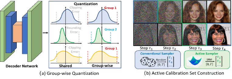
Figure 1: (a) Existing methods leverage shared quantization functions for activation discretization across different timesteps with significant quantization errors, while we divide timesteps into groups with specific rounding functions for each partition. (b) Conventional methods construct calibration set by randomly selecting timesteps for image generation with ineffective supervision, and we actively sample the timesteps based on the structural risk minimization (SRM) principle.

2 Related Work

Efficient diffusion models: Diffusion models achieve more satisfying quality and diversity in image generation compared with GAN, while the generation efficiency is significantly decreased due to the iterative noise evaluation process with long timesteps. The denoising diffusion probabilistic model (DDPM) [9] leverages a forward pass for noise perturbation and a reverse process for image denoising. Existing methods mainly focus on leveraging a shorter sampling path without sizable performance degradation, which can be divided into two categories including convergence speedup and sampling path selection. Convergence speedup methods aim to discretize the stochastic differential equations (SDE) or the ordinary differential equations (ODE) with minimized discretization errors. Song et al. [30] modeled the diffusion model with a non-Markov process that considers the original images for noise perturbation, where the convergence for image generation speeds up sizably. Bao et al. [2] formulated an analytic form of variance and KL divergence based on a pre-trained score-based model that simultaneously enhanced the log-likelihood and the generation speed. Sampling path selection usually chooses partial timesteps in the denoising process regarding the learning objectives. Watson et al. [38] searched the best $K$ sampling timesteps for noise evaluation via dynamic programming, where the goal was to maximizing the evidence lower bound (ELBO) in the reverse process. Due to the inconsistent performance between the training ELBO and the generation quality, they further presented Kernel Inception Distance (KID) [37] as the optimization objective to differentiably search the sampling timesteps. In this paper, we aim to reduce the complexity of single-step denoising process by quantization, which is orthogonal to the acceleration techniques of sampling path shortening.

Network quantization: Network quantization has aroused extensive interests in computer vision due to the significant reduction in storage and computational cost, because the full-precision variables are substituted by quantized values and the multiply-add (MAC) operations are replaced by integer arithmetics. Quantization-aware training (QAT) [22; 4; 36; 33; 34; 40] finetunes the quantized network with the dataset that is the same as the training set of full-precision models. Wang et al.[35] enforce the self-attention rank by minimizing the distance between the self-attention in quantized and real-valued transformers with adaptive concentration degree. Due to the inaccessibility of the full training set and the extremely high training cost, post-training quantization (PTQ) [23; 24; 8; 19] that optimizes the rounding functions with a small calibration set is more practical in realistic applications. Choukroun et al. [5] minimized the $l_{2}$ distance between the quantized and full-precision tensors to avoid obvious task performance degradation, and Zhao et al. [44] duplicated the channels with outliers and halved the value so that the clipping loss could be reduced without increasing the rounding errors. Liu et al. [23] preserved the relative ranking orders of the self-attention in vision transformers to prevent information loss in post-training quantization, and explored mixed-precision quantization strategy according to the nuclear norm of attention map and features. Zero-shot PTQ further extends the limits that efficiently quantize neural networks without any real image data. Cai et al. [3] optimized the pixel values of the generated images to enforce the statistics of sample batches to mimic the batch normalization (BN) layers in the full-precision networks. Li et al. [20] further extended the zero-shot PTQ framework to transformer architectures by diversifying the self-attention of different patches with defined patch similarity metrics. As Shang et al. [29] and Li et al. [18] observed, different activation distribution across timesteps and the effectiveness change of calibration images acquired in various timesteps amplify the quantization errors in existing methods. To avoid the overfitting of the step-wise quantization caused by limited calibration samples, we present the group-wise quantization for diffusion models across timesteps with significantly reduced learnable parameters. Meanwhile, different from [29] that manually assigned the timestep index for calibration generation, we generalize the structural risk minimization principle to discover the optimal timestep.

3 Approach

In this section, we first introduce the preliminaries of post-training quantization for diffusion models and then detail the group-wise quantization across generation timesteps with the differentiable search framework. Finally, we demonstrate the timestep selection for calibration image generation according to the structural risk minimization principle.

3.1 Post-training Quantization for Diffusion Models

Diffusion models leverage a forward pass to impose noise on images and a reverse pass to transform Gaussian noise into an image for generation. Denoting the real data as $\bm{x}_{0}$ and the latent image at the $t_{th}$ step as $\bm{x}_{t}$, the probability of the forward process can be represented as follows:

$$q(\bm{x}_{t}|\bm{x}_{t-1})=\mathcal{N}(\bm{x}_{t}|\sqrt{1-\beta_{t}}\bm{x}_{t-1},\beta_{t}\bm{I}),$$ (1)

where $\beta_{t}$ means the variance schedule at the $t_{th}$ step that indicates the imposed Gaussian noise to the latent image. When the total number of forward steps denoted as $T$ becomes large enough, the latent image $\bm{x}_{T}$ can be regarded as the standard Gaussian noise. We leverage an approximated condition distribution $p_{\theta}(\bm{x}_{t-1}|\bm{x}_{t})$ to generate the latent image in the reverse process due to the intractability of the true distribution $q(\bm{x}_{t-1}|\bm{x}_{t})$, where the approximated distribution is parameterized by the neural networks with weight $\theta$:

$$p_{\theta}(\bm{x}_{t-1}|\bm{x}_{t})=\mathcal{N}(\bm{x}_{t-1}|\bm{\mu}_{\theta,t}(\bm{x}_{t}),\bm{\Sigma}_{\theta,t}(\bm{x}_{t})).$$ (2)

The training process aims to minimize the negative log-likelihood with the evidence lower bound optimization in variational inference:

$$L_{VLB}=\mathbb{E}_{q(\bm{x}_{0:T})}[\log\frac{q(\bm{x}_{1:T}|\bm{x}_{0})}{p_{\theta}(\bm{x}_{0:T})}]\geqslant-\mathbb{E}_{q(\bm{x}_{0})}\log\bm{p}_{\theta}(\bm{x}_{0}).$$ (3)

In the practical applications, iterative noise estimation process is implemented with the diffusion model for content generation, and the heavy computational cost of the reverse phase disables the deployment in resource-constrained devices such as mobile phones and robots. To accelerate the denoising process for each reverse step, post-training quantization leverages a small calibration set to learn the rounding function parameters for weights and activations of the decoder, where the quantization function can be represented as follows:

$$\hat{x}=s\cdot\Phi(\left[x/s\right],z_{min},z_{max}),$$ (4)

where $[\cdot]$ means the rounding function to the nearest integer and $\Phi$ is the clipping operation that regularizes the element into the range from $z_{min}$ to $z_{max}$. The quantization scale parameter $s$ indicates the interval between adjacent rounding points. As empirically demonstrated in [29], the activation distribution varies significantly across different timesteps during the reverse process, and the shared rounding functions usually cause severe quantization errors for image generation. Moreover, randomly selecting the timestep to generate latent images for calibration set construction fails to provide sufficient information for generalizable quantization function learning.

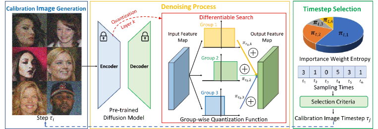
Figure 2: The overall pipeline of our method. The calibration images are generated according to the selected timesteps, and activations in the pre-trained diffusion models are parallelly quantized by rounding functions of all groups. The output feature maps are acquired by adding the quantized value with the importance weights, where the quantization parameters and the importance weights are jointly optimized. The importance weight entropy and the sampling times are considered in the timestep selection criteria to decide the timestep for calibration image generation in the next round.

3.2 Group-wise Quantization across Time Steps

Since the activation distribution changes significantly across timesteps, discretizing the full-precision intermediate features in similar value range with the same quantization functions can reduce the quantization errors. We first describe the group-wise quantization scheme and then illustrate the differentiable group assignment of timesteps.

Shared quantization functions may cause large clipping errors for widely distributed activations and rounding errors for narrowly distributed ones. Directly assigning specific rounding functions for network activations in each timestep leads to overfitting in optimization because of the limited calibration samples, and quantizing activations in the timestep where optimal quantization range is similar with the same rounding functions can achieve better trade-off between the quantization accuracy and rounding function generalizability. Assuming partitioning all $T$ timesteps into $C$ groups, the activation quantization strategy can be written in the following:

$$\hat{x}=s_{c(i)}\cdot\Phi(\left[x/s_{c(i)}\right],z_{min}^{c(i)},z_{max}^{c(i)}),$$ (5)

where $c(i)$ represents the assigned group for the activations in the $i_{th}$ timestep. Meanwhile, $s_{c(i)}$, $z_{min}^{c(i)}$ and $z_{max}^{c(i)}$ respectively stand for the scale parameter, the lower bound and the upper bound of quantization for the activations in the $i_{th}$ timestep. Assigning the optimal group indexes for different timesteps is critical in group-wise quantization to reduce the quantization errors without obvious computation overhead. Since enumerating assignment permutation is NP-hard to find the optimal solution, we extend the differentiable search framework to efficiently partition the timesteps with minimal quantization errors. In the differentiable search, the latent images are quantized by all quantization functions, whose output values are summed with learnable importance weights to form the input for the next layer in the diffusion model:

$$\hat{x}=\sum_{c=1}^{C}\pi_{c}s_{c}\cdot\Phi(\left[x/s_{c}\right],z_{min}^{c},z_{max}^{c}),$$ (6)

where $\pi_{c}$ means the importance weight of the quantization function for the $c_{th}$ group with the normalization $\sum_{c=1}^{C}\pi_{c}=1$. When the training process completes, the rounding function with the largest importance weight is selected to be the search results for group-wise quantization. Despite the noise estimation loss of diffusion models, we also enforce the importance weights to approach zero or one by minimizing the entropy to avoid discretization errors in rounding function selection. The overall optimization objective is written as follows:

$$J=J_{d}+\lambda J_{e}=\mathbb{E}_{t,\bm{x}_{0},\bm{\epsilon}}\left[||\bm{\epsilon}-\bm{\epsilon}_{\theta}(\sqrt{\overline{\alpha}_{t}}\bm{x}_{0}+\sqrt{1-\overline{\alpha}_{t}}\bm{\epsilon},t)||^{2}\right]+\lambda\mathbb{E}_{t}\sum_{c=1}^{C}-\pi_{t,c}\log\pi_{t,c},$$ (7)

where $J_{d}$ and $J_{e}$ respectively represent the simplified variational lower bound of diffusion model objective and the discretization minimization loss in differentiable search, and the hyperparameter $\lambda$ balances the importance of different terms. $\mathbb{E}$ means the variable expectation and $\pi_{t,c}$ demonstrates the importance weights of the quantization function for the $c_{th}$ group in the $t_{th}$ timestep. The noise $\bm{\epsilon}$ from standard Gaussian distribution is approximated by the predicted noise $\bm{\epsilon}_{\theta}$ in the optimization objective. The diffusion parameter $\overline{\alpha}_{t}=\prod_{i-1}^{t}1-\beta_{i}$ controls the strength of noise in diffusion. We jointly update the parameters in quantization functions and the importance weights until convergence or achieving the maximal iteration steps, and the discretized hypernetwork is directly employed to generate images efficiently.

3.3 TimeStep Selection for Calibration Image Generation

The pipeline of post-training quantization for iterative reverse process in diffusion models differs significantly from that in conventional vision models. Leveraging latent images in all timesteps leads to unbearable training cost for quantization function learning, and latent images in adjacent timesteps can only offer redundant information for parameter optimization. On the contrary, randomly select part of the timesteps usually fails to provide sufficient supervision that is representative to demonstrate the real distribution of the latent images. Therefore, it is desirable to actively sample the timesteps to generate latent images for quantization parameter learning with effective guidance. We first introduce the extension of structural risk minimization principle to active timestep selection, and then formulate the selection criteria that can be feasibly computed.

Structural risk minimization principle minimizes the upper bound of the true risk on unseen data distribution, where the bound can be written as follows for a dataset containing $n$ samples with the probability at least $1-\delta$:

$$E(J(x))\leqslant\overline{E(J(x))}+2R_{n}(\mathcal{F})+\sqrt{\frac{\ln 1/\delta}{n}},$$ (8)

where $E(J(x))$ and $\overline{E(J(x))}$ respectively illustrate the true expectation of the risk $J$ for real data distribution $x$ and the empirical expectation of that for sampled data from $x$, and $R_{n}(\mathcal{F})$ is the Rademacher complexity over the function class $\mathcal{F}$. The SRM principle requires the data to be sampled from i.i.d. distribution, while the latent images in selected timesteps should be more informative and representative. Therefore, we rewrite the SRM principle in the following way, where the detailed formulation is in the supplementary material:

$$E(J)\leqslant\overline{E_{T}(J)}+MMD(p(X),p(X_{s}))+\mathcal{R}_{0},$$ (9)

where we omit the data distribution $x$ for simplicity. $\overline{E_{T}(J)}$ denotes the empirical risk of the latent images of selected timesteps for noise estimation, and $\mathcal{R}_{0}$ demonstrates the complexity of the diffusion model in the reverse process. $X$ and $X_{s}$ stand for the distribution of latent images generated in all timesteps and the selected ones. The maximal mean discrepancy between two distributions $p(X)$ and $p(X_{s})$ is represented as $MMD(p(X),p(X_{s}))$ which demonstrates the generalization ability of the calibration sets for quantization learning. The first criteria acquired by worst-case empirical risk of sampled latent images is formulated as follows for timesteps selection :

$$\min\overline{E_{T}(J)}=\min\limits_{\theta,\mathcal{S}^{{}^{\prime}}}\sum_{\bm{x}_{t}\in\mathcal{S}}J+\sup_{\bm{\epsilon}}\sum_{\bm{x}_{t}\in\mathcal{S}^{{}^{\prime}}}J,$$ (10)

where $\mathcal{S}$ and $\mathcal{S}^{{}^{\prime}}$ respectively represent the images in the calibration set and potential calibration data in query, and $J$ is the optimization objective defined in (7). The first term aims to train the highly quantified diffusion model with the constructed calibration sets.

Since the original latent $\bm{x}_{T}$ is randomly sampled from standard Gaussian distribution without bias, the objective $J_{d}$ does not affect the worst-case empirical risk with different timesteps. The variance of $J_{e}$ influences the worst-case empirical risk across timesteps, because the entropy of the importance weights of group-wise quantization functions changes with the timesteps. Therefore, the criteria $s_{1}$ from the empirical risk minimization can be transformed to selecting the timestep with the highest entropy of importance weights as $s_{1}=\sum_{c=1}^{C}-\pi_{t,c}\log\pi_{t,c}$. The definition of maximal mean discrepancy can be written as follows, where we denote $\bm{\epsilon}_{\theta}(\sqrt{\overline{\alpha}_{t}}\bm{x}_{0}+\sqrt{1-\overline{\alpha}_{t}}\bm{\epsilon},t)$ as $\bm{\epsilon}_{\theta}(\bm{x}_{0},t)$ for simplicity:

$$\min MMD(p(X),p(X_{s}))=\min||\frac{1}{|\mathcal{S}\cup\mathcal{S}^{{}^{\prime}}|}\sum_{\bm{x}_{t}\in\mathcal{S}\cup\mathcal{S}^{{}^{\prime}}}\bm{\epsilon}_{\theta}(\bm{x}_{0},t)-\frac{1}{|U/\mathcal{S}^{{}^{\prime}}|}\sum_{\bm{x}_{t}\in U/\mathcal{S}^{{}^{\prime}}}\bm{\epsilon}_{\theta}(\bm{x}_{0},t)||,$$ (11)

where $U$ means the full set containing all original latent and timesteps for calibrate image selection, and $|\cdot|$ represents the number of elements in the set. Because the estimated noise of the samples in the full set is intractable, we utilize the number of sampling times to approximate the maximal mean discrepancy that is empirically verified in the supplementary material. For the timestep when we sample a large number of latent images for calibration set construction, the maximal mean discrepancy becomes low as we acquire sufficient information of the latent image distribution in this timestep. Therefore, we expect to select latent images in the timestep with few sampling times to further minimize the maximal mean discrepancy with high marginal benefits. The criteria $s_{2}$ from the maximal mean discrepancy is obtained by counting the number of sampling times as $s_{2}=1/N_{t}$, where $N_{t}$ represents the number of sampling times for the $t_{th}$ timestep in calibration set construction. The overall timestep selection criteria can be written as follows:

$$\max s=\max\limits_{t}s_{1}+\frac{1}{\eta}s_{2}$$ (12)

where $\eta$ is a hyperparameter to balance the importance of empirical risk and maximal mean discrepancy. With the optimally selected timesteps, the generated calibration images can provide effective supervision for quantization function learning, which can be well generalized in deployment.

4 Experiments

In this section, we first introduce the implementation details of our method. We then conduct ablation studies to evaluate the effectiveness of the group-wise quantization and the optimal timestep selection for calibration image generation, and analyze the influence of hyperparameters on generation quality and model complexity. Finally, we compare our method with the state-of-the-art post-training quantization frameworks in diffusion models to show our superiority.

4.1 Implementation Details

We utilize the diffusion frameworks for post-training quantization including DDIM [30] and LDMs [27] with their pre-trained weights, which require 100 iterative denoising timesteps for image generation in most experiments. We set the bitwidth of quantized weight and activation to 6 and 8 to evaluate our method in different quality-efficiency trade-offs and utilized the uniform quantization scheme where the interval between adjacent rounding points was equal. For group-wise quantization across different timesteps, we partitioned all timesteps into eight groups in most experiments. We followed the initialization of the quantization function parameters in [18] for the baseline methods and our ADP-DM, where we minimized the $l_{p}$ distance [25; 39] between the full-precision and quantized activations to optimize the value range for clipping. The hyperparameters $\lambda$ in the objective of differentiable search and $\eta$ in the timestep selection criteria were set to 0.8 and 1.5 respectively.

For the parameter learning in differentiable search, we generated 1024 images for hyper-network learning where the batchsize was assigned with 64 for calibration set construction. The learning rate was initialized to $3e^{-3}$ and $5e^{-3}$ for 6 and 8-bit diffusion models and ended up with $1e^{-5}$ for all bitwidth settings with 0.05 decaying strategy. The quantization function parameters and the importance weights were jointly updated for 10 epochs in the differentiable search, and the acquired group-wise quantization function was directly employed for image generation.

Table 1: Effects of the number of timestep partitions in the group-wise quantization. C-Error and G-Error depict the quantization errors of activations in calibration and generation respectively.

Bitwidth	Group	C-Error	G-Error	FID$\downarrow$
W8A8	1	1.16	1.22	5.32
	4	0.87	0.93	4.73
	8	0.79	0.82	4.24
	16	0.75	0.86	4.29
W6A6	1	1.92	2.03	9.73
	4	1.88	1.76	7.10
	8	1.57	1.68	6.57
	16	1.52	1.74	6.77

Table 2: Different timestep sampling strategies for calibration set construction across various sizes of calibration images. WBAB depicts the weights and activations are quantized to B-bit.

Method	Bitwidth	Size of Calibration Set
		256	512	1024
Random	W8A8	5.64	5.34	5.41
	W6A6	10.12	9.18	8.92
Heuristic	W8A8	5.56	5.27	5.21
	W6A6	10.19	9.03	8.83
Active	W8A8	4.46	4.49	4.24
	W6A6	11.73	7.83	6.57

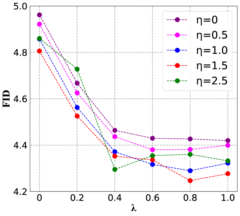
Figure 3: The generation quality w.r.t. different hyperparameters $\lambda$ and $\eta$.

4.2 Ablation Study

In order to investigate the influence of the group-wise quantization for network activations across different timesteps, we vary the number of groups with different trade-offs between quantization accuracy and rounding function generalizability. To show the effectiveness of our active timestep selection for calibration set generation, we compare our strategy with various sampling techniques. Meanwhile, we modified the hyperparameter $\lambda$ and $\eta$ to demonstrate the effect of the discretization loss in rounding function selection and the maximal mean discrepancy in timestep selection criteria. All experiments in the ablation study were conducted with the $32\times 32$ cifar-10 dataset and the DDIM diffusion framework.

Performance w.r.t. the number of timestep groups: Dividing the timesteps into more groups can reduce the clipping and rounding errors for differently distributed activations, while may result in the rounding function overfitting due to the limited calibration samples and large-scale learnable parameters. Table 4.1 illustrates the FID score, Inception Score (IS), and the number of network parameters (Param.) for our method that partitions the timesteps into different numbers of groups. Observing the FID and IS for different group partition settings, we conclude that the dividing the timesteps into several groups outperform both the shared quantization policy and the step-wise rounding functions. Therefore, we assign the number of groups for timestep partition to 8 in the rest experiments to achieve the optimal trade-off between quantization accuracy and rounding function generalizability.

Performance w.r.t. different timestep sampling strategies for calibration set construction: We compare our active timestep sampling strategy for calibration set generation with random and heuristic sampling policies [29]. Random sampling assigns an integer number drawn from uniform distribution from zero to the maximal time steps $T$, and heuristic sampling determines the timestep from a Gaussian distribution $\mathcal{N}(\mu,\frac{T}{2})$ where $\mu$ is less than $\frac{T}{2}$. Table 4.1 shows the generation quality for different timestep sampling methods across various sizes of the calibration set. Our active sampling strategy outperforms the random and heuristic sampling policies by a large margin, and the advantage is more obvious for calibration sets with small sizes because informative samples are extremely important for post-training quantization in the scenario without sufficient images.

Performance w.r.t. hyperparameters $\lambda$ and $\eta$: The hyperparameter $\lambda$ controls the importance of the discretization loss in group-wise quantization function selection in the objective of differentiable search, and $\eta$ balances the empirical risk and the maximal mean discrepancy in the timestep selection. Figure 3 depicts the FID for different hyperparameter settings, where the medium value for both parameters achieves the highest generation quality. The model performance is more sensitive to the hyperparameter $\lambda$ because the importance weights of quantization functions in different groups usually have similar distribution as one-hot vector, and slight change to $\lambda$ leads to large perturbation to the overall objective in differentiable search due to the logarithm.

4.3 Comparison with the State-of-the-art Methods

In this section, we compare our method with the state-of-the-art post-training quantization frameworks including LSQ [7] and those specifically designed for diffusion models including PTQ4DM [29] and Q-diffusion [18]. The FID and IS of the baseline methods are acquired by implementing the officially released code or our re-implementation. For fair comparison of all listed methods, we leverage the rounding function in LSQ for quantization and de-quantization, and generate images with 100 iterative steps.

Table 3: Comparisons with the state-of-the-arts on unconditional image generation for DDIM diffusion models across various datasets and bitwidth setting.

Method	Bitwidth	Cifar-10		CelebA		LSUN-Bedroom		LSUN-Church
		IS$\uparrow$	FID$\downarrow$	IS$\uparrow$	FID$\downarrow$	IS$\uparrow$	FID$\downarrow$	IS$\uparrow$	FID$\downarrow$
Baseline	FP	9.07	4.23	2.61	6.49	2.45	6.39	2.76	10.98
LSQ	W8A8	8.74	13.78	2.29	15.02	2.13	16.95	2.58	28.49
PTQ4DM		8.82	5.69	2.43	6.44	2.23	7.48	2.76	10.98
Q-Diffusion		8.87	4.78	2.41	6.60	2.27	7.04	2.72	12.72
ADP-DM		9.07	4.24	2.58	6.07	2.55	6.46	2.84	9.04
LSQ	W6A6	8.34	35.96	1.94	78.37	1.68	122.45	1.87	131.78
PTQ4DM		8.72	11.28	2.13	24.96	2.11	16.85	2.48	32.85
Q-Diffusion		8.76	9.19	2.16	23.37	2.09	17.57	2.52	33.77
ADP-DM		9.06	6.57	2.30	16.86	2.30	15.72	2.63	24.75

Results on unconditional generation: Unconditional generation samples a random variable for diffusion models to yield images with similar distribution of the training datasets. We evaluate our data-free post-training quantization methods on $32\times 32$ Cifar-10 [13], $64\times 64$ CelebA [21], $256\times 256$ LSUN-Church Outdoor and LSUN-Bedroom datasets [42] for DDIM frameworks, and evaluate for LDMs diffusion frameworks on $256\times 256$ CelebA-HQ [14], LSUN-Church Outdoor and LSUN-Bedroom datasets, where the generalization quality and efficiency are reported in Table 3 and Table 4 respectively. LSQ learns the optimal quantization step sizes with minimized discretization errors, while the shared quantization policy across timesteps in diffusion models leads to significant quantization loss. PTQ4DM and Q-diffusion employ the step-wise quantization functions to minimize the quantization errors of the diversely distributed activations, and presents heuristic criteria to sample timesteps. However, the optimization of large-scale learnable parameters face the challenges of overfitting due to the very limited calibration samples, and the data-independent calibration set construction cannot guarantee the optimality of the calibration images. As a result, our method outperforms PTQ4DM by 0.32 (2.55 vs. 2.23) and 1.02 (6.46 vs. 7.48) for IS and FID in LSUN-Bedroom respectively. The computational cost keeps the same for baseline methods and our ADP-DM due to the stored rounding parameters. The advantage of our method becomes more obvious for 6-bit diffusion models because quantization errors and calibration sample informativeness are more important for networks with low capacity.

Results on conditioned image generation: Conditioned image generation synthesizes images according to text including class names or descriptions. For class-conditional image generation, we discretize the LDMs model that is pre-trained on the $256\times 256$ class-conditional ImageNet [6] dataset, where the guidance strength is set to 3.0 to balance the generation quality and diversity. Table 4 shows the quantitative experimental results for different post-training quantization methods, while our method increases the FID and IS by 1.01 (11.58 vs. 12.59) and 17.38 (179.13 vs. 161.75) respectively compared with the state-of-the-art method PTQ4DM. For description-conditional image generation, Figure 4 demonstrates some examples of the text prompts images that are generated by different quantized Stable Diffusion models, where our method can still acquire plausible images with high-quality details with weights and activations in low bitwidths. Since conditioned image generation is widely adopted in many realistic multimedia applications, our method is practical to deploy large pre-trained diffusion models on mobile devices under limited resource constraint with satisfying generation quality.

Table 4: The generation quality on unconditional (U) and class-conditional (C) image synthesis for LDMs diffusion models across different datasets and bitwidths.

Method	Bitwidth	CelebA-HQ (U)		Bedroom (U)		Church (U)		ImageNet (C)
		IS$\uparrow$	FID$\downarrow$	IS$\uparrow$	FID$\downarrow$	IS$\uparrow$	FID$\downarrow$	IS$\uparrow$	FID$\downarrow$
Baseline	FP	3.27	6.08	2.29	3.43	2.70	4.08	180.84	11.89
LSQ	W8A8	3.01	9.75	2.13	8.11	2.50	7.10	154.06	13.26
PTQ4DM		3.11	8.57	2.21	4.75	2.52	5.29	161.75	12.59
Q-Diffusion		3.08	8.61	2.19	4.67	2.53	4.87	166.05	12.78
ADP-DM		3.22	6.30	2.35	3.88	2.69	4.02	179.13	11.58
LSQ	W6A6	2.09	129.84	1.34	122.45	1.82	135.61	115.71	40.77
PTQ4DM		2.80	19.53	2.08	11.10	2.46	11.05	140.86	13.68
Q-Diffusion		2.87	18.39	2.11	10.10	2.47	10.90	146.41	13.94
ADP-DM		3.09	16.73	2.27	9.88	2.67	6.90	178.64	11.58

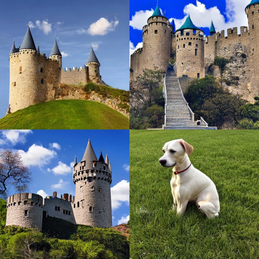
(a) Full Precision

(b) ADP-DM(6-bit)

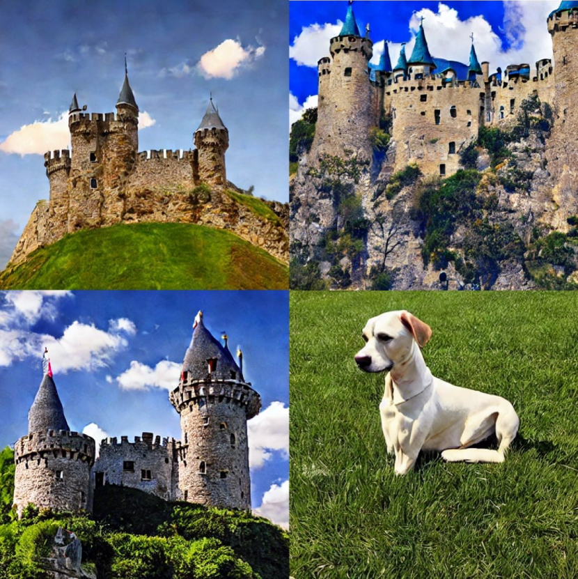
(c) PTQ4DM(6-bit)

Figure 4: The images generated by quantized Stable Diffusion models and the corresponding text prompts, where different post-training quantization methods are employed.

5 Conclusion

In this paper, we have presented a data-free post-training quantization method of diffusion model for efficient image generation. We design a differentiable search framework that assigns the optimal partition for each timestep in the reverse process, where network activations in different timesteps are discretized with group-wise quantization functions for rounding error minimization. By generalizing the structural risk minimization principle, we select the optimal timestep for calibration image construction to provide effective supervision in quantization parameter learning. Extensive experiments demonstrate that our methods achieve higher generation quality than the state-of-the-art post-training quantization methods across diffusion models with various architectures. Our current method mainly contains the following limitation. The efficient computation of structural risk minimization principle is not sufficiently precise compared with the true value and the most informative samples may be excluded in calibration set construction, which is left as the future work for diffusion model quantization.

Broader Impacts

The proposed framework considerably reduces quantization error and provides the possibility for accurately low-bit deployment for pre-trained diffusion models on edge devices including mobile devices and robots. The fast denoising ability of quantized diffusion model may leads to powerful application in image edition, super-resolution and many others.

A Formulation of (9)

Structural risk minimization principle minimizes the upper bound of the true risk on unseen data distribution, where the bound can be written as follows for a dataset containing $n$ samples with the probability at least $1-\delta$:

$$E(J(x))\leqslant\overline{E(J(x))}+2R_{n}(\mathcal{F})+\sqrt{\frac{\ln 1/\delta}{n}},$$ (13)

where $E(J(x))$ and $\overline{E(J(x))}$ respectively illustrate the true expectation of the risk $J$ for real data distribution $x$ and the empirical expectation of that for sampled data from $x$, and $R_{n}(\mathcal{F})$ is the Rademacher complexity over the function class $\mathcal{F}$. The SRM principle requires the data to be sampled from i.i.d. distribution, while the latent images in selected timesteps should be more informative and representative. In order to extend the SRM principle in active timestep selection, we omitted $x$ to reformulate the risk bound inequality:

$$E(J)\leqslant(E(J)-E_{T}(J))+\overline{E_{T}(J)}+\mathcal{R}_{0},$$ (14)

where $E(J)$ and $E_{T}(J)$ are the true risk and empirical risk of all latent images. $\mathcal{R}_{0}=2R_{n}(\mathcal{F})+\sqrt{\frac{\ln 1/\delta}{n}}$ demonstrates the complexity of the diffusion model in the reverse process. In diffusion models, the data $x$ consists of input samples $z$ and target samples $e$, we can rewrite the first term of (14) as follows:

$$E(J)-E_{T}(J) =\int p(z|z\in X)\int J\cdot p(e|z)dzde-\int p(z|z\in X_{s})\int J\cdot p(e|z)dzde$$ (15)

$$=\int g(z)p(z|z\in X)dz-\int g(z)p(z|z\in X_{s})dz,$$

where $X$ and $X_{s}$ are the distribution of latent images generated in all timesteps and the selected ones respectively. As $g(z)=\int J\cdot p(e|z)de$ is bounded and measurable, a bounded and continuous function $\hat{g}(z)$ can guarantee the boundness of (15):

$$E(J)-E_{T}(J) \leqslant\sup_{\hat{g}(z)}[\int g(z)p(X)dz-\int g(z)p(X_{s})dz]$$ (16)

$$=MMD(p(X),p(X_{s})),$$

where we rewrite $p(z|z\in X)$ as $p(X)$ for simplicity. $MMD(p(X),p(X_{s}))$ represents the maximum mean discrepancy between distribution $p(X)$ and $p(X_{s})$. Finally, we rewrite the SRM principle in the following way:

$$E(J)\leqslant\overline{E_{T}(J)}+MMD(p(X),p(X_{s}))+\mathcal{R}_{0},$$ (17)

where we omit the data distribution $x$ for simplicity. $\overline{E_{T}(J)}$ denotes the empirical risk of the latent images of selected timesteps for noise estimation.

B Empirical Verification about (10)

The definition of maximal mean discrepancy can be written as follows, where we denote $\bm{\epsilon}_{\theta}(\sqrt{\overline{\alpha}_{t}}\bm{x}_{0}+\sqrt{1-\overline{\alpha}_{t}}\bm{\epsilon},t)$ as $\bm{\epsilon}_{\theta}(\bm{x}_{0},t)$ for simplicity:

$$\min MMD(p(X),p(X_{s}))=\min||\frac{1}{|\mathcal{S}\cup\mathcal{S}^{{}^{\prime}}|}\sum_{\bm{x}_{t}\in\mathcal{S}\cup\mathcal{S}^{{}^{\prime}}}\bm{\epsilon}_{\theta}(\bm{x}_{0},t)-\frac{1}{|U/\mathcal{S}^{{}^{\prime}}|}\sum_{\bm{x}_{t}\in U/\mathcal{S}^{{}^{\prime}}}\bm{\epsilon}_{\theta}(\bm{x}_{0},t)||,$$ (18)

where $U$ means the full set containing all original latent and timesteps for calibrate image selection, and $|\cdot|$ represents the number of elements in the set. we utilize the number of sampling times to approximate the maximal mean discrepancy as the estimated noise of the samples in the full set is intractable. The criteria $s_{2}$ from the maximal mean discrepancy is obtained by counting the number of sampling times as $s_{2}=1/N_{t}$, where $N_{t}$ represents the number of sampling times for the $t_{th}$ timestep in calibration set construction. Figure 5 empirically verifies the negative correlation property of $MMD(p(X),p(X_{s}))$ and $s_{2}$ with 128 calibration samples across timesteps, which demonstrate the rationality of approximation, as we expect to select latent images in the timestep with few sampling times $N_{t}$ to further minimize the maximal mean discrepancy with high marginal benefits.

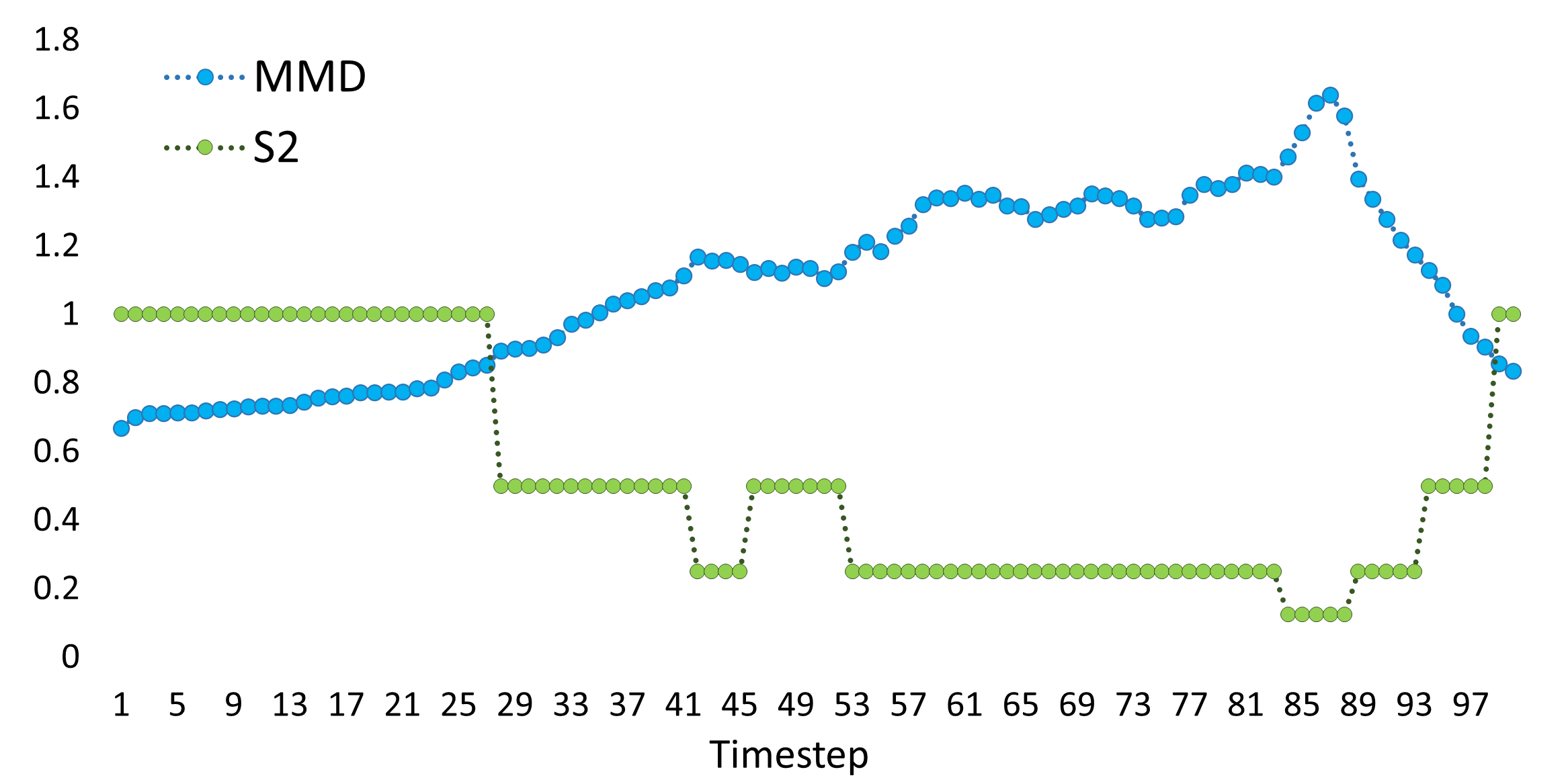
Figure 5: Empirical verification about $MMD(p(X),p(X_{s}))$ and $s_{2}$. We sample 128 samples for calibration set and calculate $MMD$ and $s_{2}$ for each timestep to demonstrate the correlation.

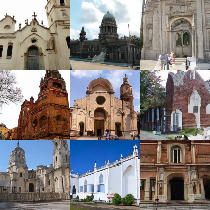
(a) Full Precision

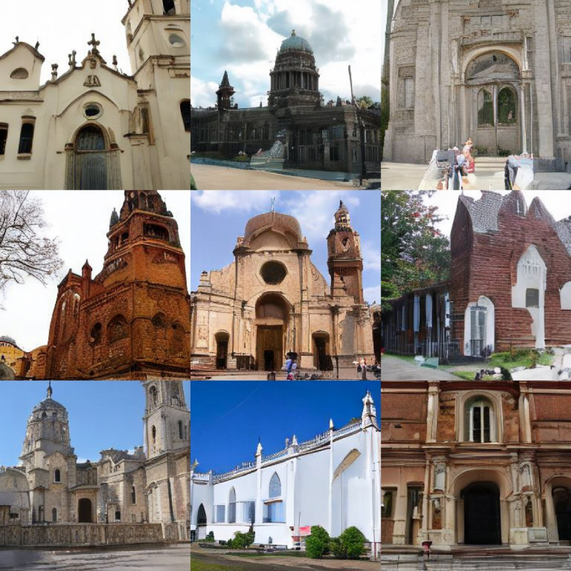
(b) ADP-DM(6-bit)

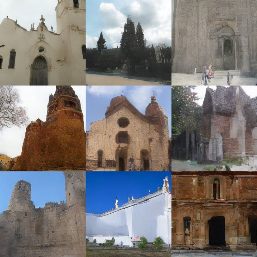
(c) PTQ4DM(6-bit)

Figure 6: $256\times 256$ LSUN-Church samples from 100 step LDMs in 6-bit with different post-training quantization methods.

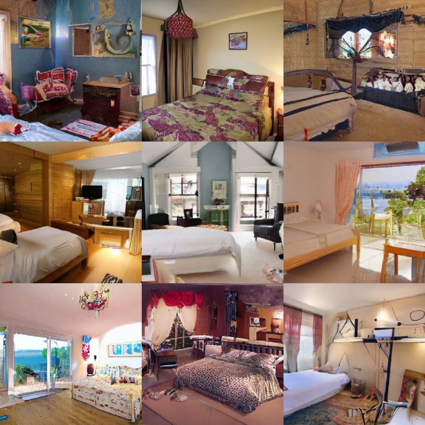
(a) Full Precision

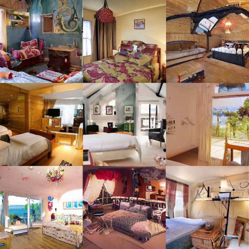
(b) ADP-DM(6-bit)

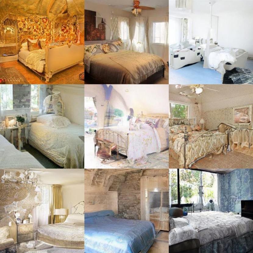
(c) PTQ4DM(6-bit)

Figure 7: $256\times 256$ LSUN-Bedroom samples from 100 step LDMs in 6-bit with different post-training quantization methods.

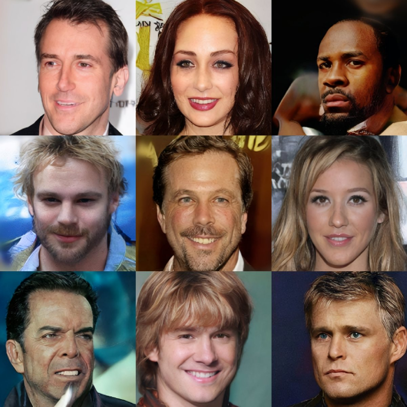
(a) Full Precision

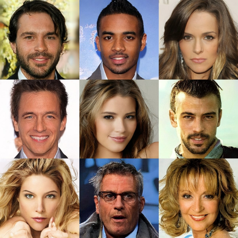
(b) ADP-DM(6-bit)

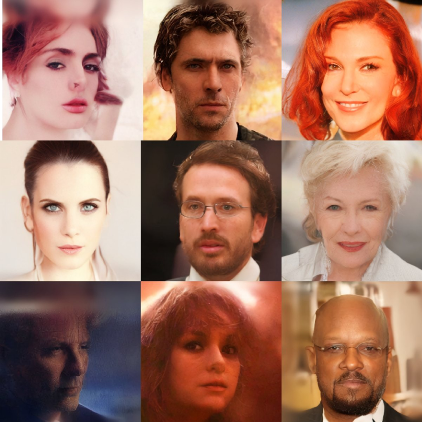
(c) PTQ4DM(6-bit)

Figure 8: $256\times 256$ CelebA-HQ samples from 100 step LDMs in 6-bit with different post-training quantization methods.

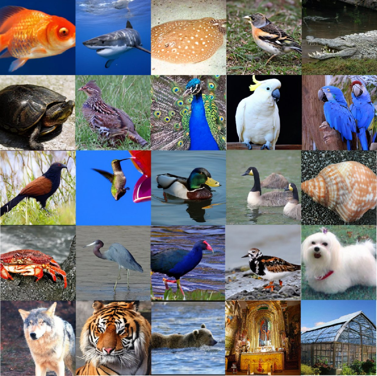
Figure 9: $256\times 256$ ImageNet samples from 100 step LDMs in 6-bit with ADP-DM.

C Samples

Additional samples: We show more samples generated by different 6-bit quantized diffusion models in Figure 6 (Church), Figure 7 (Bedroom), Figure 8 (CelebA-HQ), and Figure 9 (ImageNet). Compared with the conventional quantization method, our ADP-DM can still achieve high-quality details in plausible images with weights and activations in low bitwidths, which is semblable to the full precision ones.

References

- [1] Omri Avrahami, Dani Lischinski, and Ohad Fried. Blended diffusion for text-driven editing of natural images. In CVPR, pages 18208–18218, 2022.
- [2] Fan Bao, Chongxuan Li, Jun Zhu, and Bo Zhang. Analytic-dpm: an analytic estimate of the optimal reverse variance in diffusion probabilistic models. arXiv preprint arXiv:2201.06503, 2022.
- [3] Yaohui Cai, Zhewei Yao, Zhen Dong, Amir Gholami, Michael W Mahoney, and Kurt Keutzer. Zeroq: A novel zero shot quantization framework. In CVPR, pages 13169–13178, 2020.
- [4] Jungwook Choi, Zhuo Wang, Swagath Venkataramani, Pierce I-Jen Chuang, Vijayalakshmi Srinivasan, and Kailash Gopalakrishnan. Pact: Parameterized clipping activation for quantized neural networks. arXiv preprint arXiv:1805.06085, 2018.
- [5] Yoni Choukroun, Eli Kravchik, Fan Yang, and Pavel Kisilev. Low-bit quantization of neural networks for efficient inference. In ICCVW, pages 3009–3018, 2019.
- [6] Jia Deng, Wei Dong, Richard Socher, Li-Jia Li, Kai Li, and Li Fei-Fei. Imagenet: A large-scale hierarchical image database. In CVPR, pages 248–255, 2009.
- [7] Steven K Esser, Jeffrey L McKinstry, Deepika Bablani, Rathinakumar Appuswamy, and Dharmendra S Modha. Learned step size quantization. arXiv preprint arXiv:1902.08153, 2019.
- [8] Jun Fang, Ali Shafiee, Hamzah Abdel-Aziz, David Thorsley, Georgios Georgiadis, and Joseph H Hassoun. Post-training piecewise linear quantization for deep neural networks. In ECCV, pages 69–86, 2020.
- [9] Jonathan Ho, Ajay Jain, and Pieter Abbeel. Denoising diffusion probabilistic models. NeurIPS, 33:6840–6851, 2020.
- [10] Hengyuan Hu, Rui Peng, Yu-Wing Tai, and Chi-Keung Tang. Network trimming: A data-driven neuron pruning approach towards efficient deep architectures. arXiv preprint arXiv:1607.03250, 2016.
- [11] Itay Hubara, Matthieu Courbariaux, Daniel Soudry, Ran El-Yaniv, and Yoshua Bengio. Binarized neural networks. NeurIPS, 29, 2016.
- [12] Alexia Jolicoeur-Martineau, Ke Li, Rémi Piché-Taillefer, Tal Kachman, and Ioannis Mitliagkas. Gotta go fast when generating data with score-based models. arXiv preprint arXiv:2105.14080, 2021.
- [13] Alex Krizhevsky, Geoffrey Hinton, et al. Learning multiple layers of features from tiny images. 2009.
- [14] Cheng-Han Lee, Ziwei Liu, Lingyun Wu, and Ping Luo. Maskgan: Towards diverse and interactive facial image manipulation. In Proceedings of the IEEE/CVF Conference on Computer Vision and Pattern Recognition, pages 5549–5558, 2020.
- [15] Junghyup Lee, Dohyung Kim, and Bumsub Ham. Network quantization with element-wise gradient scaling. In CVPR, pages 6448–6457, 2021.
- [16] Haoying Li, Yifan Yang, Meng Chang, Shiqi Chen, Huajun Feng, Zhihai Xu, Qi Li, and Yueting Chen. Srdiff: Single image super-resolution with diffusion probabilistic models. Neurocomputing, 479:47–59, 2022.
- [17] Muyang Li, Ji Lin, Chenlin Meng, Stefano Ermon, Song Han, and Jun-Yan Zhu. Efficient spatially sparse inference for conditional gans and diffusion models. arXiv preprint arXiv:2211.02048, 2022.
- [18] Xiuyu Li, Long Lian, Yijiang Liu, Huanrui Yang, Zhen Dong, Daniel Kang, Shanghang Zhang, and Kurt Keutzer. Q-diffusion: Quantizing diffusion models. arXiv preprint arXiv:2302.04304, 2023.
- [19] Yuhang Li, Ruihao Gong, Xu Tan, Yang Yang, Peng Hu, Qi Zhang, Fengwei Yu, Wei Wang, and Shi Gu. Brecq: Pushing the limit of post-training quantization by block reconstruction. arXiv preprint arXiv:2102.05426, 2021.
- [20] Zhikai Li, Liping Ma, Mengjuan Chen, Junrui Xiao, and Qingyi Gu. Patch similarity aware data-free quantization for vision transformers. In ECCV, pages 154–170, 2022.
- [21] Ziwei Liu, Ping Luo, Xiaogang Wang, and Xiaoou Tang. Deep learning face attributes in the wild. In Proceedings of the IEEE international conference on computer vision, pages 3730–3738, 2015.
- [22] Zechun Liu, Wenhan Luo, Baoyuan Wu, Xin Yang, Wei Liu, and Kwang-Ting Cheng. Bi-real net: Binarizing deep network towards real-network performance. IJCV, 128:202–219, 2020.
- [23] Zhenhua Liu, Yunhe Wang, Kai Han, Wei Zhang, Siwei Ma, and Wen Gao. Post-training quantization for vision transformer. NeurIPS, 34:28092–28103, 2021.
- [24] Markus Nagel, Rana Ali Amjad, Mart Van Baalen, Christos Louizos, and Tijmen Blankevoort. Up or down? adaptive rounding for post-training quantization. In ICML, pages 7197–7206. PMLR, 2020.
- [25] Yury Nahshan, Brian Chmiel, Chaim Baskin, Evgenii Zheltonozhskii, Ron Banner, Alex M Bronstein, and Avi Mendelson. Loss aware post-training quantization. Machine Learning, 110(11-12):3245–3262, 2021.
- [26] Alex Nichol, Prafulla Dhariwal, Aditya Ramesh, Pranav Shyam, Pamela Mishkin, Bob McGrew, Ilya Sutskever, and Mark Chen. Glide: Towards photorealistic image generation and editing with text-guided diffusion models. arXiv preprint arXiv:2112.10741, 2021.
- [27] Robin Rombach, Andreas Blattmann, Dominik Lorenz, Patrick Esser, and Björn Ommer. High-resolution image synthesis with latent diffusion models. In Proceedings of the IEEE/CVF Conference on Computer Vision and Pattern Recognition, pages 10684–10695, 2022.
- [28] Chitwan Saharia, Jonathan Ho, William Chan, Tim Salimans, David J Fleet, and Mohammad Norouzi. Image super-resolution via iterative refinement. TPAMI, 2022.
- [29] Yuzhang Shang, Zhihang Yuan, Bin Xie, Bingzhe Wu, and Yan Yan. Post-training quantization on diffusion models. arXiv preprint arXiv:2211.15736, 2022.
- [30] Jiaming Song, Chenlin Meng, and Stefano Ermon. Denoising diffusion implicit models. arXiv preprint arXiv:2010.02502, 2020.
- [31] Yang Song, Jascha Sohl-Dickstein, Diederik P Kingma, Abhishek Kumar, Stefano Ermon, and Ben Poole. Score-based generative modeling through stochastic differential equations. arXiv preprint arXiv:2011.13456, 2020.
- [32] Xuan Su, Jiaming Song, Chenlin Meng, and Stefano Ermon. Dual diffusion implicit bridges for image-to-image translation. In ICLR, 2022.
- [33] Ziwei Wang, Jiwen Lu, Ziyi Wu, and Jie Zhou. Learning efficient binarized object detectors with information compression. IEEE Transactions on Pattern Analysis and Machine Intelligence, 44(6):3082–3095, 2021.
- [34] Ziwei Wang, Jiwen Lu, and Jie Zhou. Learning channel-wise interactions for binary convolutional neural networks. IEEE Transactions on Pattern Analysis & Machine Intelligence, 43(10):3432–3445, 2021.
- [35] Ziwei Wang, Changyuan Wang, Xiuwei Xu, Jie Zhou, and Jiwen Lu. Quantformer: Learning extremely low-precision vision transformers. IEEE Transactions on Pattern Analysis and Machine Intelligence, 2022.
- [36] Ziwei Wang, Han Xiao, Yueqi Duan, Jie Zhou, and Jiwen Lu. Learning deep binary descriptors via bitwise interaction mining. IEEE Transactions on Pattern Analysis and Machine Intelligence, 2022.
- [37] Daniel Watson, William Chan, Jonathan Ho, and Mohammad Norouzi. Learning fast samplers for diffusion models by differentiating through sample quality. In International Conference on Learning Representations, 2022.
- [38] Daniel Watson, Jonathan Ho, Mohammad Norouzi, and William Chan. Learning to efficiently sample from diffusion probabilistic models. arXiv preprint arXiv:2106.03802, 2021.
- [39] Xiuying Wei, Ruihao Gong, Yuhang Li, Xianglong Liu, and Fengwei Yu. Qdrop: randomly dropping quantization for extremely low-bit post-training quantization. arXiv preprint arXiv:2203.05740, 2022.
- [40] Xiuwei Xu, Ziwei Wang, Jie Zhou, and Jiwen Lu. Binarizing sparse convolutional networks for efficient point cloud analysis. arXiv preprint arXiv:2303.15493, 2023.
- [41] Serin Yang, Hyunmin Hwang, and Jong Chul Ye. Zero-shot contrastive loss for text-guided diffusion image style transfer. arXiv preprint arXiv:2303.08622, 2023.
- [42] Fisher Yu, Ari Seff, Yinda Zhang, Shuran Song, Thomas Funkhouser, and Jianxiong Xiao. Lsun: Construction of a large-scale image dataset using deep learning with humans in the loop. arXiv preprint arXiv:1506.03365, 2015.
- [43] Chenglong Zhao, Bingbing Ni, Jian Zhang, Qiwei Zhao, Wenjun Zhang, and Qi Tian. Variational convolutional neural network pruning. In CVPR, pages 2780–2789, 2019.
- [44] Ritchie Zhao, Yuwei Hu, Jordan Dotzel, Chris De Sa, and Zhiru Zhang. Improving neural network quantization without retraining using outlier channel splitting. In ICML, pages 7543–7552, 2019.
- [45] Yunshan Zhong, Mingbao Lin, Gongrui Nan, Jianzhuang Liu, Baochang Zhang, Yonghong Tian, and Rongrong Ji. Intraq: Learning synthetic images with intra-class heterogeneity for zero-shot network quantization. In CVPR, pages 12339–12348, 2022.