Distributed Hierarchical Distribution Control for Very-Large-Scale Clustered Multi-Agent Systems

Abstract

As the scale and complexity of multi-agent robotic systems are subject to a continuous increase, this paper considers a class of systems labeled as Very-Large-Scale Multi-Agent Systems (VLMAS) with dimensionality that can scale up to the order of millions of agents. In particular, we consider the problem of steering the state distributions of all agents of a VLMAS to prescribed target distributions while satisfying probabilistic safety guarantees. Based on the key assumption that such systems often admit a multi-level hierarchical clustered structure - where the agents are organized into cliques of different levels - we associate the control of such cliques with the control of distributions, and introduce the Distributed Hierarchical Distribution Control (DHDC) framework. The proposed approach consists of two sub-frameworks. The first one, Distributed Hierarchical Distribution Estimation (DHDE), is a bottom-up hierarchical decentralized algorithm which links the initial and target configurations of the cliques of all levels with suitable Gaussian distributions. The second part, Distributed Hierarchical Distribution Steering (DHDS), is a top-down hierarchical distributed method that steers the distributions of all cliques and agents from the initial to the targets ones assigned by DHDE. Simulation results that scale up to two million agents demonstrate the effectiveness and scalability of the proposed framework. The increased computational efficiency and safety performance of DHDC against related methods is also illustrated. The results of this work indicate the importance of hierarchical distribution control approaches towards achieving safe and scalable solutions for the control of VLMAS. A video with all results is available here.

I Introduction

Multi-agent systems in robotics are experiencing an increasing popularity with several significant applications such as multi-robot coordination [11], navigating fleets of vehicles [28], guiding teams of UAVs [37] and swarm robotics [6], to name only a few. As the scale and complexity of such systems are continuously growing, a great requirement has emerged for developing algorithmic frameworks that benefit from a distributed structure, high computational efficiency, low communication requirements, and therefore, scalability. In addition, as uncertainty is an integral component of multi-agent systems, associating such methods with safety guarantees remains of paramount importance.

Most of the existing literature in multi-robot control, has considered systems that range from a handful of units to hundreds or thousands of agents. Some notable approaches can be found in the fields of optimal control [24, 25, 32, 39], path planning [8, 13, 26], swarm robotics [6, 21, 22, 30] and multi-agent reinforcement learning [12, 14, 16, 38]. Nevertheless, empirical demonstrations show that the scalability of most methods from the previous classes is practically limited in the order of a few thousands of robots.

This paper considers a class of systems, labeled as Very-Large-Scale Multi-Agent Systems (VLMAS), that can scale up to the order of millions of robots. To also account for potential uncertainties in VLMAS, all agents are modeled with stochastic dynamics. To our best knowledge, the literature for addressing the control of such systems in a safe, distributed and scalable manner while operating under uncertainty is very scarce. The key insight of this work is that VLMAS often admit a hierarchical clustered structure (Fig. 1) where robots are arranged into cliques, which are then organized into greater cliques etc. Such a structure is highly suitable for the proposed direction of hierarchical distribution control.

Figure 1: A VLMAS with a hierarchical clustered structure of $L$ levels. Level $L$ corresponds to individual robots and their distributions (green). All robots are organized into level-($L-1$) cliques (orange) which are then also organized into level-($L-2$) cliques and so on, up to level-$1$ cliques (blue).

Multi-robot control approaches that exploit such hierarchies appear to be quite few in the literature. A multi-robot navigation method that used hierarchical clustering to identify the formation of groups of robots and guide them to their targets was proposed in [2]. Furthermore, a distributed algorithm for the coordination of clusters of robots was recently presented in [15]. While these works have hinted towards the potential of distributed hierarchical control in robotics, their approaches were still only applicable to small-scale multi-robot teams and unrelated to the control of distributions.

As safety requirements in robotics and control are of great significance, covariance steering (CS) theory has recently emerged as a promising approach for guiding the state distribution of a system to prescribed targets while providing probabilistic safety guarantees [3, 4, 10, 20]. Successful robotics applications can be found in trajectory optimization [5, 35], path planning [23], flight control [7, 17, 27], multi-robot systems [31, 33] and robotic manipulation [18], to name a few. While the main barrier for applying CS methods for multi-agent stochastic control was due to their significant computational requirements, recent distributed optimization based approaches [31, 33] have shown that CS is a viable option for multi-agent systems. Nevertheless, the scalability of the aforementioned methods appears to be practically limited to systems with tens or hundreds of agents. In addition, to our best knowledge, combining CS with the control of the distributions of clusters of agents has not been considered yet in the literature.

In this paper, we aspire to surpass the appearing limitations of current CS approaches, by exploiting the fact that VLMAS systems can be subject to a hierarchical clustered structure. In such a multi-level hierarchical setup, the agents are organized into cliques, which are then organized into greater cliques, and so on. Our key insight lies in the fact that CS theory can also be utilized for the control of such cliques in addition to the control of individual agents. Based on this fact, we introduce a novel distributed method for the control of VLMAS, named Distributed Hierarchical Distribution Control (DHDC). The DHDC framework consists of two separate sub-frameworks. The first one, Distributed Hierarchical Distribution Estimation (DHDE), associates all cliques with suitable Gaussian distributions that satisfy the hierarchical structure, while the second one, Distributed Hierarchical Distribution Steering (DHDS), utilizes CS to drive the distributions of all cliques and agents towards their assigned targets. The specific contributions of this work can be listed as follows:

1. We illustrate how covariance steering theory can be fused with the control of clusters of agents that are linked through a hierarchical structure.

2. We propose DHDE, a bottom-up hierarchical distributed approach for estimating the optimal random distributions to be associated with the cliques of each level of the hierarchy.

3. We propose DHDS, a top-down hierarchical distributed approach for steering the distributions of all cliques and agents to their targets, by exploiting the information acquired with DHDE.

4. We demonstrate the effectiveness and scalability of the proposed approaches through simulation experiments on systems with up to two million agents.

To our best knowledge, the proposed approach is one of the few existing methods for the distributed and safe control of stochastic systems in the VLMAS scale. In addition, DHDC greatly outperforms the scalability of all current CS approaches for multi-agent control, and therefore, paves the way for the application of CS theory to robotic systems of a much larger scale. Furthermore, this work highlights the potential of hierarchical distributed optimization methods that utilize distribution characteristics for the control of large-scale multi-agent systems.

II Problem Statement

II-A Notation

The set of $n\times n$ symmetric positive semi-definite (definite) matrices is denoted with $\mathbb{S}_{n}^{+}$ ($\mathbb{S}_{n}^{++}$). Given two matrices $A,B\in\mathbb{R}^{n\times n}$, the matrix inequality $A\succeq B$ refers to $A-B\in\mathbb{S}_{n}^{+}$. Given a random variable (r.v.) $x\in\mathbb{R}^{n}$, its expectation and covariance are given by $\mathbb{E}[x]\in\mathbb{R}^{n}$ and $\mathbb{C}\mathbb{O}\mathbb{V}[x]\in\mathbb{S}_{n}^{+}$, respectively. If a r.v. $x\in\mathbb{R}^{n}$ is such that $x\sim\pazocal{N}(\mu,\Sigma)$, then $x$ is subject to a multivariate Gaussian distribution with mean $\mu=\mathbb{E}[x]$ and covariance $\Sigma=\mathbb{C}\mathbb{O}\mathbb{V}[x]$. In addition, $x\in\pazocal{E}_{\theta}[\mu,\Sigma]$ implies that $x\in\mathbb{R}^{n}$ lies within the $\theta$-probability confidence ellipsoid of $\pazocal{N}(\mu,\Sigma)$, i.e., $\pazocal{E}_{\theta}[\mu,\Sigma]:(x-\mu)^{\mathrm{T}}\Sigma^{-1}(x-\mu)\leq\alpha$, where $\alpha=f_{\chi^{2},\nu}^{-1}(\theta)$ and $f_{\chi^{2},\nu}^{-1}(\cdot)$ is the inverse cumulative distribution function of the chi-square distribution with $\nu$ degrees of freedom. The Kullback–Leibler (KL) divergence of a probability distribution $\pazocal{P}$ from another distribution $\pazocal{Q}$ is denoted with $\mathbb{D}_{\mathrm{KL}}(\pazocal{P}\|\pazocal{Q})$. Furthermore, the cardinality of a set $\pazocal{A}$ is given by $|\pazocal{A}|$. Finally, $\llbracket a,b\rrbracket$ denotes the integer set $[a,b]\cap\mathbb{Z}$ for any $a,b\in\mathbb{R}$ with $a\leq b$.

II-B Problem Formulation

Let us consider a VLMAS given by the set $\pazocal{R}=\{1,\dots,M\}$, where $M$ is the total number of agents. Each agent $i\in\pazocal{R}$ is subject to the following homogeneous discrete-time, stochastic, linear dynamics

$$x_{i,k+1}=Ax_{i,k}+Bu_{i,k}+w_{i,k},$$ (1)

where $x_{i,k}\in\mathbb{R}^{n_{x}}$ and $u_{i,k}\in\mathbb{R}^{n_{u}}$ are the state and control of the $i$-th agent at time $k$, $w_{i,k}\in\mathbb{R}^{n_{x}}$ is process noise such that $w_{i,k}\sim\pazocal{N}(0,W)$ with $W\in\mathbb{S}_{n_{x}}^{+}$, and $A\in\mathbb{R}^{n_{x}\times n_{x}}$, $B\in\mathbb{R}^{n_{x}\times n_{u}}$. If we denote the time horizon with $N$, i.e., $k\in\llbracket 0,N\rrbracket$, then the full state, control and noise sequences of agent $i$ are given by $x_{i}=[x_{i,0};\dots;x_{i,N}]$, $u_{i}=[u_{i,0};\dots;u_{i,N-1}]$ and $w_{i}=[w_{i,0};\dots;w_{i,N-1}]$, respectively. All initial states $x_{i,0}$ are subject to $x_{i,0}\sim\pazocal{N}(\mu_{i,0},\Sigma_{i,0})$, where $\mu_{i,0}\in\mathbb{R}^{n_{x}}$ and $\Sigma_{i,0}\in\mathbb{S}_{n_{x}}^{++}$ are known.

Let us now introduce the VLMAS distribution control problem. The main objective is to steer the distributions of the terminal states $x_{i,N}$ of all agents to prescribed target distributions $\pazocal{N}(\mu_{i,\mathrm{f}},\Sigma_{i,\mathrm{f}})$ with $\mu_{i,\mathrm{f}}\in\mathbb{R}^{n_{x}}$ and $\Sigma_{i,\mathrm{f}}\in\mathbb{S}_{n_{x}}^{++}$. This can be achieved by enforcing the following constraints

$$\mathbb{E}[x_{i,N}] =\mu_{i,\mathrm{f}},$$ (2)

$$\mathbb{C}\mathbb{O}\mathbb{V}[x_{i,N}] \preceq\Sigma_{i,\mathrm{f}},$$ (3)

for every agent $i\in\pazocal{R}$. Furthermore, the position of each agent in space is given by $p_{i,k}=Hx_{i,k}\in\mathbb{R}^{n_{p}}$, with $H\in\mathbb{R}^{n_{p}\times n_{x}}$ defined accordingly. To simplify exposition, in this work, we consider agents that operate on a 2D plane, i.e., $n_{p}=2$. Nevertheless, all proposed ideas are readily extendable for 3D multi-robot systems. The following probabilistic inter-agent collision avoidance constraints must also be satisfied between all agents,

$$\mathbb{P}\left(\|p_{i,k}-p_{j,k}\|_{2}\geq d_{\mathrm{inter}}\right)\geq\theta,\quad\forall i,j\in\pazocal{R},\ i\neq j,$$ (4)

for all $k\in\llbracket 0,N\rrbracket$, where $d_{\mathrm{inter}}$ is the minimum allowed distance between two agents and $\theta\in(0.5,1)$. In addition, we assume the existence of a set $\pazocal{O}=\{1,\dots,O\}$ of circle obstacles and consider the following probabilistic safety constraints

$$\mathbb{P}\left(\|p_{i,k}-p_{o}\|_{2}\geq d_{\mathrm{obs}}+r_{o}\right)\geq\theta,\quad\forall i\in\pazocal{R},\ \forall o\in\pazocal{O},$$ (5)

for all $k\in\llbracket 0,N\rrbracket$, where $r_{o}$ is the radius of obstacle $o\in\pazocal{O}$ and $d_{\mathrm{obs}}$ is the minimum allowed distance between an agent and an obstacle. Finally, all agents also aim to minimize their control effort through the following individual costs

$$J_{i}(u_{i})=\sum_{k=0}^{N-1}\mathbb{E}[u_{i,k}^{\mathrm{T}}Ru_{i,k}],\quad i\in\pazocal{R}.$$ (6)

where $R\in\mathbb{S}_{n}^{++}$. Consequently, the VLMAS distribution control problem can be formulated as follows.

Problem 1 (VLMAS Distribution Control Problem).

Find the optimal control input sequences $u_{i}^{*},\ \forall i\in\pazocal{R}$, such that

$$\{u_{i}^{*}\}_{i\in\pazocal{R}}=\operatornamewithlimits{argmin}\sum_{i\in\pazocal{R}}J_{i}(u_{i})$$

$$~{}~{}~{}\mathrm{s.t.}\quad\eqref{linear dynamics},\eqref{terminal mean constraint},\eqref{terminal cov constraint},\eqref{collision avoidance constraints},\eqref{obs avoidance constraints}.$$

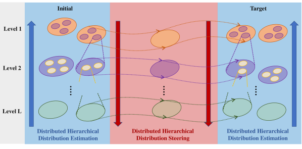
Figure 2: The DHDC framework consists of two parts. The first part (DHDE) is a bottom-up approach that estimates the initial and target random distributions that correspond to all cliques of levels $\ell\in\llbracket 1,L-1\rrbracket$, such that the assumed hierarchical clustered structure is satisfied. The second part (DHDS) is a top-down approach that steers the distributions of the cliques/agents of all levels based on the initial and target distributions provided by DHDE.

II-C Hierarchical Clustered Structure

This work focuses on VLMAS that are subject to a known hierarchical clustered structure (Fig. 1). This hierarchy consists of $L$ levels with each level denoted with $\ell\in\{1,\dots,L\}$. The bottom level $\ell=L$ corresponds to individual agents. All agents are organized into level-$(L-1)$ cliques $\pazocal{C}_{i}^{L-1}\in\pazocal{R}^{L-1}$, which are then organized into level-$(L-2)$ cliques $\pazocal{C}_{i}^{L-2}\in\pazocal{R}^{L-2}$, and so on, where $\pazocal{R}^{\ell}$ denotes the set of all cliques in each level $\ell\in\llbracket 1,L\rrbracket$. If by convention, we let the level-$L$ cliques $\pazocal{C}_{i}^{L}$ correspond to individual agents $i\in\pazocal{R}$, i.e., $\pazocal{R}^{L}\equiv\pazocal{R}$, then the aforementioned structure can be formally stated as follows.

Assumption 1 (Hierarchical Clustered Structure).

For all levels $\ell\in\llbracket 2,L\rrbracket$, it holds that for every clique $\pazocal{C}_{i}^{\ell}\in\pazocal{R}^{\ell}$, there exists a clique $\pazocal{C}_{a}^{\ell-1}\in\pazocal{R}^{\ell-1}$ such that

$$\pazocal{C}_{i}^{\ell}\subseteq\pazocal{C}_{a}^{\ell-1}.$$ (7)

In other words, every clique in level $\ell$ belongs to a “parent” clique of level $\ell-1$. Furthermore, for all levels $\ell\in\llbracket 1,L\rrbracket$, it holds that

$$\pazocal{C}_{i}^{\ell}\cap\pazocal{C}_{j}^{\ell}=\emptyset,\quad\forall\pazocal{C}_{i}^{\ell},\pazocal{C}_{j}^{\ell}\in\pazocal{R}^{\ell},\ i\neq j,$$ (8)

i.e., the intersection between cliques of the same level is always the empty set.

Furthermore, to lighten the notation, given a clique $\pazocal{C}_{i}^{\ell}$, we consider the statements $\pazocal{C}_{i}^{\ell}\in\pazocal{A}$ and $i\in\pazocal{A}$ to be equivalent for any arbitrary set $\pazocal{A}$. A direct consequence of Assumption 1 is the following.

Corollary 1.

For all levels $\ell\in\llbracket 2,L\rrbracket$, every clique $\pazocal{C}_{i}^{\ell}$ only has one “parent” clique $\pazocal{C}_{a}^{\ell-1}$.

Subsequently, we introduce the notion of neighbor cliques. Given a clique $\pazocal{C}_{i}^{\ell}$, the set of its neighbor cliques is defined as $\mathfrak{n}[\pazocal{C}_{i}^{\ell}]$. Of course, if $\ell\in\llbracket 2,L\rrbracket$, then all cliques $\pazocal{C}_{j}^{\ell}$ with $j\in\mathfrak{n}[\pazocal{C}_{i}^{\ell}]$ have the same “parent” clique as $\pazocal{C}_{i}^{\ell}$, i.e., if $\pazocal{C}_{i}^{\ell}\subseteq\pazocal{C}_{a}^{\ell-1}$, then $\pazocal{C}_{j}^{\ell}\subseteq\pazocal{C}_{a}^{\ell-1}$, $\forall j\in\mathfrak{n}[\pazocal{C}_{i}^{\ell}]$. The set of cliques $\pazocal{C}_{j}^{\ell}$ that include $\pazocal{C}_{i}^{\ell}$ as a neighbor clique is defined with $\mathfrak{m}[\pazocal{C}_{i}^{\ell}]$, i.e., if $\pazocal{C}_{j}^{\ell}$ is such that $i\in\mathfrak{n}[\pazocal{C}_{j}^{\ell}]$, then $j\in\mathfrak{m}[\pazocal{C}_{i}^{\ell}]$. Note that it is not required that $\mathfrak{n}[\pazocal{C}_{i}^{\ell}]\equiv\mathfrak{m}[\pazocal{C}_{i}^{\ell}]$.

Next, all necessary communication assumptions are stated. First, we formulate the basic communication capabilities of every agent which are only limited in exchanging information with their neighboring agents within the same level-$(L-1)$ clique.

Assumption 2 (Basic Communication Capabilities).

Every agent $i\in\pazocal{R}$ (or just $\pazocal{C}_{i}^{L}\in\pazocal{R}$) is able to exchange information with all agents $j\in\mathfrak{n}[\pazocal{C}_{i}^{L}]\cup\mathfrak{m}[\pazocal{C}_{i}^{L}]$.

Note that compared to the potential scale of a VLMAS, and assuming that neighbor sets would be relatively small, this is considered to be a minor communication requirement. In the following assumption, we establish how communication between different cliques materializes, by assigning increased communication capabilities to specific agents.

Assumption 3 (Increased Communication Capabilities).

For all levels $\ell\in\llbracket 1,L-1\rrbracket$, in each clique $\pazocal{C}_{i}^{\ell}$, there exists one agent with “level-$\ell$ communication capabilities”, or more briefly a “level-$\ell$ agent”. Each level-$\ell$ agent is able to exchange information with:

• all level-$(\ell+1)$ agents of the cliques $\pazocal{C}_{n}^{\ell+1}$ such that $\pazocal{C}_{n}^{\ell+1}\subseteq\pazocal{C}_{i}^{\ell}$,

• all level-$\ell$ agents that belong in $\mathfrak{n}[\pazocal{C}_{i}^{\ell}]\cup\mathfrak{m}[\pazocal{C}_{i}^{\ell}]$.

II-D Virtual States for Clique Dynamics

Finally, towards associating the control of the cliques of levels $1,\dots,L-1$, with covariance steering, we define their correspoding virtual states $x_{i}^{\ell}\in\mathbb{R}^{n_{x}}$ and controls $u_{i}^{\ell}\in\mathbb{R}^{n_{u}}$, for all $i\in\pazocal{R}^{\ell}$. Since the dynamics of all agents are homogeneous, the virtual states are modeled to follow the same dynamics as the agents,

$$x_{i,k+1}^{\ell}=Ax_{i,k}^{\ell}+Bu_{i,k}^{\ell}+w_{i,k}^{\ell},$$ (9)

where $w_{i,k}^{\ell}\sim\pazocal{N}(0,W)$. Note that this is still far from associating the control of cliques with covariance steering, since the initial and target random distributions of the cliques of all levels $\ell\in\llbracket 1,L-1\rrbracket$ are not available and require rigorous selection such that the hierarchical structure is satisfied. In the next section, we propose an approach for estimating these initial and target random distributions as Gaussian distributions $\pazocal{N}(\mu_{i,0}^{\ell},\Sigma_{i,0}^{\ell})$ and $\pazocal{N}(\mu_{i,\mathrm{f}}^{\ell},\Sigma_{i,\mathrm{f}}^{\ell})$, $\forall i\in\pazocal{R}^{\ell},\ \ell\in\llbracket 1,L-1\rrbracket$.

III Distributed Hierarchical Distribution Estimation

This section focuses on the problem of finding the optimal Gaussian distributions for representing the initial and target state configurations of the cliques $\pazocal{C}_{i}^{\ell}$, $\forall\pazocal{R}^{\ell}$, $\ell\in\llbracket 1,L-1\rrbracket$, based on the known level-$L$ distributions. We label this problem as the inter-level distribution estimation problem. Towards addressing it, we propose Distributed Hierarchical Distribution Estimation (DHDE), a hierarchical distributed approach that operates in a bottom-up fashion (Fig. 2) for estimating the desired random distributions.

III-A Single-Clique Distribution Estimation

To facilitate the exposition of our ideas, we first consider the simplified subproblem of single-clique distribution estimation, where the objective is to estimate the Gaussian distribution that best describes a clique $\pazocal{C}_{i}^{\ell}$, i.e., best captures the random state distributions of all cliques $\pazocal{C}_{n}^{\ell+1}\subseteq\pazocal{C}_{i}^{\ell}$ with a single Gaussian distribution, without considering potential overlaps in the 2D space between neighboring cliques. Furthermore, note that the distribution estimation problem has the same form, either we refer to the initial or target configurations, thus we make no distinction between the two and drop the corresponding notation.

In order to find the optimal distribution $\pazocal{N}_{i}^{\ell}=\pazocal{N}(\mu_{i}^{\ell},\Sigma_{i}^{\ell})$ for capturing all the distributions $\pazocal{N}_{n}^{\ell+1}=\pazocal{N}(\mu_{n}^{\ell+1},\Sigma_{n}^{\ell+1})$ of the cliques $\pazocal{C}_{n}^{\ell+1}$ such that $\pazocal{C}_{n}^{\ell+1}\subseteq\pazocal{C}_{i}^{\ell}$, we select the KL divergence metric $\mathbb{D}_{\mathrm{KL}}(\pazocal{N}_{n}^{\ell+1}\|\pazocal{N}_{i}^{\ell})$ to measure discrepancies between distributions. In addition, by defining the parts of the means and covariances that correspond to the position coordinates as $\bar{\mu}_{i}=H\mu_{i}$ and $\bar{\Sigma}_{i}=H\Sigma_{i}H^{\mathrm{T}}$, we impose the constraints

$$\pazocal{E}_{\theta}[\bar{\mu}_{n}^{\ell+1},\bar{\Sigma}_{n}^{\ell+1}]\subseteq\pazocal{E}_{\theta}[\bar{\mu}_{i}^{\ell},\bar{\Sigma}_{i}^{\ell}],\quad n\in\pazocal{C}_{i}^{\ell},$$ (10)

so that the assumed hierarchical clustered structure is indeed satisfied. Therefore, the single-clique distribution estimation problem can be stated for a particular clique $\pazocal{C}_{i}^{\ell}\in\pazocal{R}^{\ell}$ of a given level $\ell\in\llbracket 1,L-1\rrbracket$, as follows.

Problem 2 (Single-Clique Distribution Estimation Problem).

Find the optimal Gaussian distribution $\pazocal{N}(\mu_{i}^{\ell},\Sigma_{i}^{\ell})$ such that

$$\left\{\mu_{i}^{\ell},\Sigma_{i}^{\ell}\right\}=\operatornamewithlimits{argmin}J_{i}^{\mathrm{e}}(\mu_{i}^{\ell},\Sigma_{i}^{\ell})$$ (11a)

$$\mathrm{s.t.}\quad \pazocal{E}_{\theta}[\bar{\mu}_{n}^{\ell+1},\bar{\Sigma}_{n}^{\ell+1}]\subseteq\pazocal{E}_{\theta}[\bar{\mu}_{i}^{\ell},\bar{\Sigma}_{i}^{\ell}],\ n\in\pazocal{C}_{i}^{\ell},$$ (11b)

$$\Sigma_{i}^{\ell}\succ 0,$$ (11c)

where

$$J_{i}^{\mathrm{e}}=\sum_{n\in\pazocal{C}_{i}^{\ell}}\mathbb{D}_{\mathrm{KL}}(\pazocal{N}_{n}^{\ell+1}\|\pazocal{N}_{i}^{\ell}).$$ (12)

In the following proposition, we present a tractable optimization problem whose optimal solution provides the optimal solution of Problem 2. From now on, the level superscripts will be omitted unless not obvious from the context.

Proposition 1.

Let us introduce the auxiliary optimization variables $Q_{i}=\Sigma_{i}^{-1}$, $q_{i}=\Sigma_{i}^{-1}\mu_{i}$ and $\tau_{n}\in\mathbb{R}$, $\forall n\in\pazocal{C}_{i}^{\ell}$. The optimal solution of Problem 2 is obtained by solving the following convex optimization problem

$$~{}~{}~{}~{}~{}~{}~{}\min\hat{J}_{i}^{\mathrm{e}}(Q_{i},q_{i})$$ (13a)

$$\mathrm{s.t}\quad S_{n}(\bar{Q}_{i},\bar{q}_{i},\tau_{n})\succeq 0,\quad n\in\pazocal{C}_{i}^{\ell},$$ (13b)

$$\tau_{n}\geq 0,\quad n\in\pazocal{C}_{i}^{\ell},$$ (13c)

$$Q_{i}\succ 0,$$ (13d)

w.r.t. $Q_{i}$, $q_{i}$ and $\{\tau_{n}\}_{n\in\pazocal{C}_{i}^{\ell}}$, where

$$\hat{J}_{i}^{\mathrm{e}}(Q_{i},q_{i})=\sum_{n\in\pazocal{C}_{i}^{\ell}}-\log|Q_{i}|+\mathrm{tr}(Q_{i}\Sigma_{n})+q_{i}^{\mathrm{T}}Q_{i}^{-1}q_{i}$$

$$~{}~{}~{}~{}~{}~{}~{}~{}~{}~{}~{}~{}~{}~{}~{}~{}~{}~{}~{}~{}~{}~{}-2\mu_{n}^{\mathrm{T}}q_{i}+\mu_{n}^{\mathrm{T}}Q_{i}\mu_{n},$$ (14a)

$$S_{n}=\begin{bmatrix}S_{11}&S_{12}&0\\ S_{12}^{\mathrm{T}}&S_{22}&S_{23}\\ 0^{\mathrm{T}}&S_{23}^{\mathrm{T}}&S_{33}\end{bmatrix},$$ (14b)

$$S_{11}=-\bar{Q}_{i}+\tau_{n}\bar{\Sigma}_{n}^{-1},\ S_{12}=\bar{q}_{i}-\tau_{n}\bar{\Sigma}_{n}^{-1}\bar{\mu}_{n},$$ (14c)

$$S_{22}=\alpha+\tau_{n}\bar{\mu}_{n}^{\mathrm{T}}\bar{\Sigma}_{n}^{-1}\bar{\mu}_{n}-\alpha\tau_{n},\ S_{23}=\bar{q}_{i}^{\mathrm{T}},\ S_{33}=\bar{Q}_{i},$$

$$\bar{Q}_{i}=HQ_{i}H^{\mathrm{T}},\ \bar{q}_{i}=Hq_{i},\ \alpha=f_{\chi^{2},2}^{-1}(\theta),$$ (14d)

and setting $\mu_{i}=Q_{i}^{-1}q_{i}$ and $\Sigma_{i}=Q_{i}^{-1}$.

Proof.

The proof is provided in Section VII-A of the Supplementary Material (SM). ∎

III-B Multi-Clique Distribution Estimation

Let us now consider an extended version of the previous problem, labeled as the multi-clique distribution estimation one, where the objective is to simultaneously estimate the Gaussian distributions $\pazocal{N}_{i}^{\ell}$ of all cliques $\pazocal{C}_{i}^{\ell}$ such that $\pazocal{C}_{i}^{\ell}\subseteq\pazocal{C}_{a}^{\ell-1}$, i.e., all cliques that belong in the same parent clique $\pazocal{C}_{a}^{\ell-1}$ (or just $\pazocal{R}^{1}$ if $\ell=1$). In this case, it is also necessary to ensure that the $\theta$-probability confidence ellipses $\pazocal{E}_{\theta}[\bar{\mu}_{i}^{\ell},\bar{\Sigma}_{i}^{\ell}]$ of neighboring cliques will not overlap with each other, i.e., we also impose the following constraints

$$\pazocal{E}_{\theta}[\bar{\mu}_{i}^{\ell},\bar{\Sigma}_{i}^{\ell}]\cap\pazocal{E}_{\theta}[\bar{\mu}_{j}^{\ell},\bar{\Sigma}_{j}^{\ell}]=\emptyset,\ j\in\mathfrak{n}[\pazocal{C}_{i}^{\ell}],$$ (15)

between neighbor cliques of the same parent clique. Hence, the multi-clique distribution estimation problem can be formulated as follows.

Problem 3 (Multi-Clique Distribution Estimation Problem).

Given a parent clique $\pazocal{C}_{a}^{\ell-1}$ (or $\pazocal{R}^{1}$ if $\ell=1$), find the optimal Gaussian distributions $\pazocal{N}\left(\mu_{i}^{\ell},\Sigma_{i}^{\ell}\right)$ for all $i\in\pazocal{C}_{a}^{\ell-1}$, such that

$$\big{\{}\mu_{i}^{\ell},\Sigma_{i}^{\ell}\big{\}}_{i\in\pazocal{C}_{a}^{\ell-1}}=\operatornamewithlimits{argmin}\sum_{i\in\pazocal{C}_{a}^{\ell-1}}J_{i}^{\mathrm{e}}(\mu_{i}^{\ell},\Sigma_{i}^{\ell})$$ (16a)

$$\mathrm{s.t.}\quad \pazocal{E}_{\theta}[\bar{\mu}_{n}^{\ell+1},\bar{\Sigma}_{n}^{\ell+1}]\subseteq\pazocal{E}_{\theta}[\bar{\mu}_{i}^{\ell},\bar{\Sigma}_{i}^{\ell}],\ n\in\pazocal{C}_{i}^{\ell},$$ (16b)

$$\pazocal{E}_{\theta}[\bar{\mu}_{i}^{\ell},\bar{\Sigma}_{i}^{\ell}]\cap\pazocal{E}_{\theta}[\bar{\mu}_{j}^{\ell},\bar{\Sigma}_{j}^{\ell}]=\emptyset,\ j\in\mathfrak{n}[\pazocal{C}_{i}^{\ell}],$$ (16c)

$$\Sigma_{i}^{\ell}\succ 0,\ i\in\pazocal{C}_{a}^{\ell-1},$$ (16d)

where $J_{i}^{\mathrm{e}}(\mu_{i}^{\ell},\Sigma_{i}^{\ell})$ is the same as in Problem 2.

In the following proposition, we present an optimization problem whose optimal solution provides a suboptimal solution for Problem 3.

Proposition 2.

Let us introduce the auxiliary optimization variables $Q_{i}=\Sigma_{i}^{-1}$, $q_{i}=\Sigma_{i}^{-1}\mu_{i}$, $\phi_{i}\in\mathbb{R}$ and $\tau_{i,n}\in\mathbb{R}$, $\forall n\in\pazocal{C}_{i}^{\ell},\ \forall i\in\pazocal{C}_{a}^{\ell-1}$. A suboptimal solution for Problem 3 is obtained by solving the following optimization problem

$$~{}~{}~{}~{}~{}~{}\min\sum_{i\in\pazocal{C}_{a}^{\ell-1}}\hat{J}_{i}^{\mathrm{e}}(Q_{i},q_{i})$$ (17a)

$$\mathrm{s.t}\quad S_{i,n}(\bar{Q}_{i},\bar{q}_{i},\tau_{i,n})\succeq 0,\ n\in\pazocal{C}_{i}^{\ell},$$ (17b)

$$\tau_{i,n}\geq 0,\ n\in\pazocal{C}_{i}^{\ell},$$ (17c)

$$h_{i,j}(\bar{Q}_{i},\bar{q}_{i},\phi_{i},\bar{Q}_{j},\bar{q}_{j},\phi_{j})\leq 0,\ j\in\mathfrak{n}[\pazocal{C}_{i}^{\ell}],$$ (17d)

$$T_{i}(\bar{Q}_{i},\phi_{i})\succeq 0,$$ (17e)

$$Q_{i}\succ 0,\ i\in\pazocal{C}_{a}^{\ell-1},$$ (17f)

w.r.t. $Q_{i}$, $q_{i}$, $\{\tau_{n}\}_{n\in\pazocal{C}_{i}^{\ell}}$ and $\phi_{i}$, $\forall i\in\pazocal{C}_{a}^{\ell-1}$, where

$$h_{i,j} =r_{i}(\phi_{i})+r_{j}(\phi_{j})-\left\|\bar{Q}_{i}^{-1}\bar{q}_{i}-\bar{Q}_{j}^{-1}\bar{q}_{j}\right\|_{2},$$ (18a)

$$r_{i} =\phi_{i}^{-1/2},\ T_{i}=\bar{Q}_{i}-\phi_{i}\alpha I,$$ (18b)

$\hat{J}_{i}^{\mathrm{e}}$, $S_{i,n}$, $\bar{Q}_{i}$ and $\bar{q}_{i}$ are as in Proposition 1, and setting $\mu_{i}=Q_{i}^{-1}q_{i}$ and $\Sigma_{i}=Q_{i}^{-1}$ for every $i\in\pazocal{C}_{a}^{\ell-1}$.

Proof.

Provided in Section VII-B of the SM. ∎

Remark 1.

The optimal solution of the problem in Proposition 2 might be suboptimal - but always feasible - for Problem 3, in the sense that the constraints (17d) and (17c) formulate a “tighter” version of (16c), as shown in Section VII-B.

Note that the cost and all constraints in (17) are convex except for (17d). As explained in the next section, we address that through iterative linearization of the constraint.

III-C Distributed Hierarchical Distribution Estimation

Let us now formulate the full inter-level distribution estimation problem, whose objective is to estimate the optimal distributions $\pazocal{N}(\mu_{i}^{\ell},\Sigma_{i}^{\ell})$ of all cliques $\pazocal{C}_{i}^{\ell}\in\pazocal{R}^{\ell}$ of all levels $\ell\in\llbracket 1,L-1\rrbracket$. Of course, this problem will consist of many interconnected instances of Problem 3. In fact, the inter-level distribution estimation problem can be formulated as follows.

Problem 4 (Inter-Level Distribution Estimation Problem).

For all $\ell\in\llbracket 1,L-1\rrbracket$ and for all $a\in\pazocal{R}^{\ell-1}$ (if $\ell\geq 2)$ , find the sets of optimal Gaussian distributions $\{\pazocal{N}\left(\mu_{i}^{\ell},\Sigma_{i}^{\ell}\right)\},\ i\in\pazocal{C}_{a}^{\ell-1}$ , that solve each corresponding Problem 3.

The goal of the proposed Distributed Hierarchical Distribution Estimation (DHDE) framework is to solve Problem 4 using a bottom-up strategy, since the only a priori known distributions are the level-$L$ ones. In this direction, we propose first solving all instances of Problem 3 in Level $L-1$, then based on the acquired information, i.e. all $\pazocal{N}_{i}^{L-1}$, solve all instances of Problem 3 in Level $L-2$, to obtain all $\pazocal{N}_{i}^{L-2}$, and so on. Of course, based on the results of Section III-B, we also replace all these instances of Problem 3 with the Proposition 2 problems. Finally, to further distribute computations, we propose solving each such problem in a distributed manner using an approach based on the Alternating Direction Method of Multipliers (ADMM) [9].

Algorithm 1 DHDE Algorithm

1:Inputs: Hier_Structure, $\mu_{i}^{L},\Sigma_{i}^{L},\forall i\in\pazocal{R}$, $\theta$

2:for $\ell=L-1:-1:1$ do

3:     if $\ell>1$ then

4:         $\pazocal{A}\leftarrow\pazocal{R}^{\ell-1}$

5:     else

6:         $\pazocal{A}\leftarrow\{1\}$      

7:     for $a\in\pazocal{A}$ do (in parallel)

8:         for $i\in\pazocal{C}_{a}^{\ell-1}$ do (in parallel)

9:              All $n\in\pazocal{C}_{i}^{\ell}$ send $\mu_{n}^{\ell+1},\Sigma_{n}^{\ell+1}$ to $i$.          

10:         while Term_Criterion $==$ False do

11:              for $i\in\pazocal{C}_{a}^{\ell-1}$ do (in parallel)

12:                  $\{\tilde{Q}_{i},\tilde{q}_{i},\tilde{\phi}_{i}\}\leftarrow$ Solve (21).

13:                  All $j\in\mathfrak{m}[\pazocal{C}_{i}^{\ell}]$ send $\{Q_{i}^{j},q_{i}^{j},\phi_{i}^{j}\}$ to $i$.               

14:              for $i\in\pazocal{C}_{a}^{\ell-1}$ do (in parallel)

15:                  $\{G_{i},g_{i},z_{i}\}\leftarrow$ Update with (23).

16:                  All $j\in\mathfrak{n}[\pazocal{C}_{i}^{\ell}]$ send $\{G_{j},g_{j},z_{j}\}$ to $i$.               

17:              for $i\in\pazocal{C}_{a}^{\ell-1}$ do (in parallel)

18:                  $\{\Xi_{i},\xi_{i},y_{i}\}\leftarrow$ Update with (24).                        

19:         for $i\in\pazocal{C}_{a}^{\ell-1}$ do (in parallel)

20:              $\{\mu_{i}^{\ell},\Sigma_{i}^{\ell}\}\leftarrow$ Compute based on $Q_{i},q_{i}$.               

In order to solve problem (17) in a distributed fashion, we first need to address the coupling induced by the constraints (17d) between neighboring cliques. Hence, we define the copy variables $Q_{j}^{i}$, $q_{j}^{i}$ and $\phi_{j}^{i}$, for all $j\in\mathfrak{n}[\pazocal{C}_{i}^{\ell}]$, and subsequently the augmented variables

$$\tilde{Q}_{i} =\big{[}Q_{i};\{Q_{j}^{i}\}_{j\in\mathfrak{n}[\pazocal{C}_{i}^{\ell}]}\big{]},$$ (19a)

$$\tilde{q}_{i} =\big{[}q_{i};\{q_{j}^{i}\}_{j\in\mathfrak{n}[\pazocal{C}_{i}^{\ell}]}\big{]},$$ (19b)

$$\tilde{\phi}_{i} =\big{[}\phi_{i};\{\phi_{j}^{i}\}_{j\in\mathfrak{n}[\pazocal{C}_{i}^{\ell}]}\big{]}.$$ (19c)

Note that the addition of the copy variables might have created multiple variables for each agent. To accommodate for that, we also define the global variables $G=[\{G_{i}\}_{i\in\pazocal{C}_{a}^{\ell-1}}]$, $g=[\{g_{i}\}_{i\in\pazocal{C}_{a}^{\ell-1}}]$, $z=[\{z_{i}\}_{i\in\pazocal{C}_{a}^{\ell-1}}]$, and impose the consensus constraints

$$\tilde{Q}_{i}=\tilde{G}_{i},\ \tilde{q}_{i}=\tilde{g}_{i},\ \tilde{\phi}_{i}=\tilde{z}_{i},$$ (20)

where $\tilde{G}_{i}=[G_{i};\{G_{j}\}_{j\in\mathfrak{n}[\pazocal{C}_{i}^{\ell}]}]$, $\tilde{g}_{i}=[g_{i};\{g_{j}\}_{j\in\mathfrak{n}[\pazocal{C}_{i}^{\ell}]}]$ and $\tilde{z}_{i}=[z_{i};\{z_{j}\}_{j\in\mathfrak{n}[\pazocal{C}_{i}^{\ell}]}]$.

Next, we present the algorithm updates; for a full derivation, the reader is referred to Section VII-C of the SM. First, each level-$\ell$ agent $i$ updates its local variables $\tilde{Q}_{i}$, $\tilde{q}_{i}$ and $\tilde{\phi}_{i}$ by solving the optimization problem

$$\{\tilde{Q}_{i},\tilde{q}_{i},\tilde{\phi}_{i}\}=\operatornamewithlimits{argmin}\tilde{J}_{i}^{\mathrm{e}}(\tilde{Q}_{i},\tilde{q}_{i},\tilde{\phi}_{i})$$ (21a)

$$\mathrm{s.t}\quad S_{i,n}(Q_{i},q_{i},\tau_{i,n})\succeq 0,\ n\in\pazocal{C}_{i}^{\ell},$$ (21b)

$$\tau_{i,n}\geq 0,\ n\in\pazocal{C}_{i}^{\ell},$$ (21c)

$$\bar{h}_{i,j}(Q_{i},q_{i},\phi_{i},Q_{j}^{i},q_{j}^{i},\phi_{j}^{i})\leq 0,\ j\in\mathfrak{n}[\pazocal{C}_{i}^{\ell}],$$ (21d)

$$T_{i}(Q_{i},\phi_{i})\succeq 0,$$ (21e)

$$Q_{i}\succ 0$$ (21f)

where the augmented costs $\tilde{J}_{i}^{\mathrm{e}}(\tilde{Q}_{i},\tilde{q}_{i},\tilde{\phi}_{i})$ are given by

$$\tilde{J}_{i}^{\mathrm{e}} =\hat{J}_{i}^{\mathrm{e}}(Q_{i},q_{i})+\mathrm{tr}(\Xi_{i}^{\mathrm{T}}(\tilde{Q}_{i}-\tilde{G}_{i}))+\xi_{i}^{\mathrm{T}}(\tilde{q}_{i}-\tilde{g}_{i})$$

$$~{}~{}+y_{i}^{\mathrm{T}}(\tilde{\phi}_{i}-\tilde{z}_{i})+\frac{\rho_{Q}}{2}\|\tilde{Q}_{i}-\tilde{G}_{i}\|_{F}^{2}+\frac{\rho_{q}}{2}\|\tilde{q}_{i}-\tilde{g}_{i}\|_{2}^{2}$$

$$~{}~{}+\frac{\rho_{\phi}}{2}\|\tilde{\phi}_{i}-\tilde{z}_{i}\|_{2}^{2},$$ (22)

with $\rho_{Q},\rho_{q},\rho_{\phi}>0$ being penalty parameters and $\Xi_{i},\xi_{i},y_{i}$ being the dual variables of the corresponding constraints. In addition, we take advantage of the iterative nature of ADMM and replace $h_{i,j}(\cdot)$ in (21d) with its linear approximation $\bar{h}_{i,j}(\cdot)$ to convexify problem (21). For more details, the reader is referred to Section VII-D of the SM.

Subsequently, the components of the global variables are updated locally by each level-$\ell$ agent as follows,

$$G_{i}\leftarrow\frac{1}{|\mathfrak{m}^{\prime}[\pazocal{C}_{i}^{\ell}]|}\sum_{j\in\mathfrak{m}^{\prime}[\pazocal{C}_{i}^{\ell}]}Q_{i}^{j}$$ (23)

where $\mathfrak{m}^{\prime}[\pazocal{C}_{i}^{\ell}]=\mathfrak{m}[\pazocal{C}_{i}^{\ell}]\cup\{i\}$. The updates for $g_{i}$ and $z_{i}$ have the same form as (23) if we replace $Q_{i}^{j}$ with $q_{i}^{j}$ and $\phi_{i}^{j}$, respectively. Finally, the dual variables are updated with

$$\Xi_{i} \leftarrow\Xi_{i}+\rho_{Q}(\tilde{Q}_{i}-\tilde{G}_{i})$$ (24a)

$$\xi_{i} \leftarrow\xi_{i}+\rho_{q}(\tilde{q}_{i}-\tilde{g}_{i})$$ (24b)

$$y_{i} \leftarrow y_{i}+\rho_{\phi}(\tilde{\phi}_{i}-\tilde{z}_{i}).$$ (24c)

Note that all updates in (21), (23), (24) can be performed in parallel by each level-$\ell$ agent $i$. Therefore, all computations take place in a decentralized manner.

The DHDE algorithm with all necessary computation and communication steps is illustrated in Alg. 1. The method operates in a bottom-up fashion for $\ell=\{L-1,L-2,\dots,1\}$. For a particular level $\ell$, the first step is that all agents $n$ such that $\pazocal{C}_{n}^{\ell+1}\subseteq\pazocal{C}_{i}^{\ell}$ send $\mu_{n}^{\ell+1},\Sigma_{n}^{\ell+1}$ to the level-$\ell$ agent $i$ that corresponds to the clique $\pazocal{C}_{i}^{\ell}$ (Line 9). Then the iterative ADMM procedure starts for every different group of agents that corresponds to a clique $\pazocal{C}_{a}^{\ell-1}$ (Lines 10-18). Note that these procedures can of course take place in parallel. Focusing into a particular group of agents that belong in clique $\pazocal{C}_{a}^{\ell-1}$, the ADMM updates are performed as follows. First, each agent $i\in\pazocal{C}_{a}^{\ell-1}$ solves (21) to update its local variables $\{\tilde{Q}_{i}$, $\tilde{q}_{i},\tilde{\phi}_{i}\}$ (Line 12). Subsequently, each $i$ receives the copy variables $\{Q_{i}^{j},q_{i}^{j},\phi_{i}^{j}\}$ from all $j\in\mathfrak{m}[\pazocal{C}_{i}^{\ell}]$ (Line 13). As a result, each agent $i$ can now obtain the new iterates for $\{G_{i},g_{i},z_{i}\}$ (Line 15) through updates of the form (23). Afterwards, all agents $j\in\mathfrak{n}[\pazocal{C}_{i}^{\ell}]$ send the variables $\{G_{j},g_{j},z_{j}\}$ to each $i$ (Line 16) so that each agent $i$ updates its dual variables $\{\Xi_{i},\xi_{i},y_{i}\}$ (Line 18) with (24). Once a predefined termination criterion is satisfied, each agent $i$ computes the variables $\mu_{i}^{\ell}$ and $\Sigma_{i}^{\ell}$ (Line 20). Now that the estimates $\mu_{i}^{\ell},\Sigma_{i}^{\ell}$ have been found for all $\ell\in\pazocal{R}^{\ell}$, this procedure repeats for the above level $\ell-1$, and so on, until level $1$ is reached.

IV Distributed Hierarchical Distribution Steering

After associating all cliques of all levels with their initial and target Gaussian distributions, we proceed with addressing the problem of steering all state distributions from the initial to the target ones. We label this problem as the inter-level distribution steering one. To solve this problem, we propose a top-down hierarchical distributed method (Fig. 2) called Distributed Hierarchical Distribution Steering (DHDS).

IV-A Multi-Clique Distribution Steering

Before formulating the inter-level problem, let us again first state a subproblem that serves as the basic component of the full problem. In particular, we consider the multi-clique distribution steering problem whose objective is to steer the Gaussian distributions of (the virtual states of) all $i$ such that the cliques $\pazocal{C}_{i}^{\ell}\subseteq\pazocal{C}_{a}^{\ell-1}$, for a specific parent clique $\pazocal{C}_{a}^{\ell-1}$ and level $\ell$. Of course, in the case where $\ell=1$, we consider $\pazocal{R}^{1}$ as the parent clique. Thus, the multi-clique distribution steering problem can be formulated as follows.

Problem 5 (Multi-Clique Distribution Steering Problem).

Given a parent clique $\pazocal{C}_{a}^{\ell-1}$ (or $\pazocal{R}^{1}$ if $\ell=1$), find the optimal control sequences $u_{i}^{\ell}$ for all $i\in\pazocal{C}_{a}^{\ell-1}$, such that

$$\big{\{}u_{i}^{\ell}\big{\}}_{i\in\pazocal{C}_{a}^{\ell-1}}=\operatornamewithlimits{argmin}\sum_{i\in\pazocal{C}_{a}^{\ell-1}}J_{i}^{\mathrm{s}}(u_{i}^{\ell})$$ (25a)

$$\mathrm{s.t.}\quad x_{i,k+1}^{\ell}=Ax_{i,k}^{\ell}+Bu_{i,k}^{\ell}+w_{i,k}^{\ell},$$ (25b)

$$\mathbb{E}[x_{i,N}^{\ell}]=\mu_{i,\mathrm{f}}^{\ell},~{}\mathbb{C}\mathbb{O}\mathbb{V}[x_{i,N}^{\ell}]\preceq\Sigma_{i,\mathrm{f}}^{\ell},$$ (25c)

$$q_{i,j,k}^{\ell}(p_{i,k}^{\ell},p_{j,k}^{\ell})\geq 0,~{}j\in\mathfrak{n}[\pazocal{C}_{i}^{\ell}],$$ (25d)

$$s_{i,k}^{\ell}(p_{i,k}^{\ell})\geq 0,$$ (25e)

$$\pazocal{E}_{\theta}[\bar{\mu}_{i,k}^{\ell},\bar{\Sigma}_{i,k}^{\ell}]\subseteq\pazocal{E}_{\theta}[\bar{\mu}_{a,k}^{\ell-1},\bar{\Sigma}_{a,k}^{\ell-1}],$$ (25f)

$$k\in\llbracket 0,N\rrbracket,~{}i\in\pazocal{C}_{a}^{\ell-1},$$

where

$$J_{i}^{\mathrm{s}}(u_{i}^{\ell})=\sum_{k=0}^{N-1}\mathbb{E}[u_{i,k}^{\ell\ \mathrm{T}}Ru_{i,k}^{\ell}],$$ (26a)

$$q_{i,j,k}^{\ell}(p_{i,k}^{\ell},p_{j,k}^{\ell})=\mathbb{P}\left(\|p_{i,k}^{\ell}-p_{j,k}^{\ell}\|_{2}\geq d_{\mathrm{inter}}^{\ell}\right)-\theta,$$ (26b)

$$s_{i,k}^{\ell}(p_{i,k}^{\ell})=\mathbb{P}\left(\|p_{i,k}^{\ell}-p_{o}\|_{2}\geq d_{\mathrm{obs}}^{\ell}+r_{o}\right)-\theta.$$ (26c)

and $d_{\mathrm{inter}}^{\ell}$, $d_{\mathrm{obs}}^{\ell}$ are prespecified parameters.

In the following, we will be omitting level superscripts, unless not clear by the context.

IV-B Problem Transformation

In order to address Problem 5, we consider the affine disturbance feedback control policies proposed in [4], with

$$u_{i,k}=\bar{u}_{i,k}+L_{i,k}(x_{i,0}-\mu_{i,0})+\sum^{k-1}_{\kappa=0}K_{i,(k-1,\kappa)}w_{i,\kappa},$$ (27)

where $\bar{u}_{i,k}\in\mathbb{R}^{n_{u}}$ are the feed-forward control terms and $L_{i,k},\ K_{i,(k-1,\kappa)}\in\mathbb{R}^{n_{u}\times n_{x}}$ are feedback gain matrices. After concentrating these variables for the entire time horizon, we obtain the decision variables $\bar{u}_{i}\in\mathbb{R}^{Nn_{u}}$, $L_{i}\in\mathbb{R}^{Nn_{u}\times n_{x}}$ and $K_{i}\in\mathbb{R}^{Nn_{u}\times Nn_{x}}$, with their exact forms provided in Section VIII-A of the SM. Thus, the control sequences $u_{i}$ can be rewritten as

$$u_{i}=\bar{u}_{i}+L_{i}(x_{i,0}-\mu_{i,0})+K_{i}w_{i}.$$ (28)

If we also write the dynamics (9) in their concatenated form,

$$x_{i}=\Psi_{0}x_{i,0}+\Psi_{u}u_{i}+\Psi_{w}w_{i},$$ (29)

where the matrices $\Psi_{0}$, $\Psi_{u}$ and $\Psi_{w}$ are provided in the SM, then through (28), we obtain

$$x_{i} =\Psi_{0}x_{i,0}+\Psi_{u}\bar{u}_{i}+\Psi_{u}L_{i}(x_{i,0}-\mu_{i,0})$$

$$~{}~{}~{}~{}+(\Psi_{w}+\Psi_{u}K_{i})w_{i}.$$ (30)

Therefore, given that affine transformations preserve Gaussianity, the entire state sequence $x_{i}$ is a Gaussian vector, which implies that $x_{i,k}\sim\pazocal{N}(\mu_{i,k},\Sigma_{i,k})$, with

$$\mu_{i,k}=f_{i,k}(\bar{u}_{i}),\quad\Sigma_{i,k}=F_{i,k}(L_{i},K_{i}),$$ (31)

where the exact expressions for $f_{i,k}(\bar{u}_{i})$ and $F_{i,k}(L_{i},K_{i})$ are provided in the SM. Note that the mean states only depend on the feed-forward controls, while the state covariances only depend on the feedback matrices. This is a useful fact that we will later exploit to further increase computational efficiency.

In the following proposition, we present an new optimization problem whose optimal solution provides a suboptimal one for Problem 5.

Proposition 3.

A suboptimal solution for Problem 5 is obtained by solving the following optimization problem. In particular, given a parent clique $\pazocal{C}_{a}^{\ell-1}$ (or $\pazocal{R}^{1}$ if $\ell=1$), find the optimal decision variables $\bar{u}_{i},L_{i},K_{i}$ for all $i\in\pazocal{C}_{a}^{\ell-1}$, such that

$$\big{\{}\bar{u}_{i}, L_{i},K_{i}\big{\}}_{i\in\pazocal{C}_{a}^{\ell-1}}=\operatornamewithlimits{argmin}\sum_{i\in\pazocal{C}_{a}^{\ell-1}}\hat{J}_{i}^{\mathrm{s}}(\bar{u}_{i},L_{i},K_{i})$$ (32a)

$$\mathrm{s.t.}\quad \mathfrak{f}_{i,N}(\bar{u}_{i})=0,~{}\pazocal{F}_{i,N}(L_{i},K_{i})\succeq 0,$$ (32b)

$$\pazocal{Q}_{i,k}(L_{i},K_{i})\succeq 0,~{}\mathfrak{s}_{i,k}(\bar{u}_{i})\geq 0,$$ (32c)

$$\mathfrak{q}_{i,j,k}(\bar{u}_{i},\bar{u}_{j})\geq 0,~{}j\in\mathfrak{n}[\pazocal{C}_{i}^{\ell}],$$ (32d)

$$\mathfrak{p}_{i,k}(\bar{u}_{i})\leq 0,~{}k\in\llbracket 0,N\rrbracket,~{}i\in\pazocal{C}_{a}^{\ell-1},$$ (32e)

with

$$\hat{J}_{i}^{\mathrm{s}}=\bar{u}_{i}^{\mathrm{T}}\bar{R}\bar{u}_{i}+\mathrm{tr}(\bar{R}K_{i}WK_{i}^{\mathrm{T}}+\bar{R}L_{i}\Sigma_{i,0}L_{i}^{\mathrm{T}}),$$ (33a)

$$\mathfrak{f}_{i,N}(\bar{u}_{i})=\mu_{i,\mathrm{f}}-f_{i,N}(\bar{u}_{i}),$$ (33b)

$$\pazocal{F}_{i,N}(L_{i},K_{i})=\begin{bmatrix}\Sigma_{i,\mathrm{f}}&\Phi_{i,N}(L_{i},K_{i})\\ \Phi_{i,N}(L_{i},K_{i})^{\mathrm{T}}&I\end{bmatrix},$$ (33c)

$$\pazocal{Q}_{i,k}(L_{i},K_{i})=\begin{bmatrix}\big{(}\frac{r^{\ell}}{\sqrt{\alpha}}\big{)}^{2}I&H\Phi_{i,k}(L_{i},K_{i})\\ \Phi_{i,k}(L_{i},K_{i})^{\mathrm{T}}H^{\mathrm{T}}&I\end{bmatrix},$$ (33d)

$$\mathfrak{s}_{i,k}(\bar{u}_{i},\bar{u}_{j})=\|\bar{f}_{i,k}(\bar{u}_{i})-p_{o}\|_{2}-r^{\ell}-r_{o}-d_{\mathrm{obs}}^{\ell},$$ (33e)

$$\mathfrak{p}(\bar{u}_{i})=\|\bar{f}_{i,k}(\bar{u}_{i})-\bar{\mu}_{a,k}^{\ell-1}\|_{\hat{P}}-1\leq 0,$$ (33f)

$$\mathfrak{q}_{i,j,k}(\bar{u}_{i},\bar{u}_{j})=\|\bar{f}_{i,k}(\bar{u}_{i})-\bar{f}_{i,k}(\bar{u}_{j})\|_{2}-2r^{\ell}-d_{\mathrm{inter}}^{\ell},$$ (33g)

where $\bar{R}=\mathrm{blkdiag(R,\dots,R)}\in\mathbb{S}_{n}^{++}$ $\bar{f}_{i,k}=Hf_{i,k}$, $r^{\ell}$ is a prespecified parameter and $\Phi_{i,k}(L_{i},K_{i})$ is an affine function of $L_{i},K_{i}$, provided in Section VIII-B of the SM. The matrix $\hat{P}=\frac{1}{\alpha}U\hat{\Lambda}^{-1}U^{\mathrm{T}}$, where

$$\hat{\Lambda}=\left(\Lambda^{1/2}-\frac{r}{\sqrt{\alpha}}I\right)^{2},$$ (34)

with $[\Lambda,U]$ being the eigendecomposition of the matrix $\bar{\Sigma}_{a,k}^{\ell-1}$.

Proof.

Provided in Section VIII-B of the SM. ∎

Remark 2.

The optimal solution of the problem in Proposition 3 might be suboptimal - but always feasible - for Problem 5, since the constraints (32c)-(32d) provide a “tighter” version of (25d)-(25e), as shown in Section VIII-B.

Remark 3.

A major advantage of the problem presented in Proposition 3, is that it is separable w.r.t. the feed-forward control variables $\bar{u}_{i}$ and the feedback matrices $L_{i},K_{i}$. In addition, an inter-agent coupling only appears through the variables $\bar{u}_{i}$ - because of (32d) - and not through $L_{i},K_{i}$. As shown in the next section, these two facts can be exploited to significantly increase computational efficiency.

IV-C Distributed Hierarchical Distribution Steering

Let us now introduce the full inter-level distribution steering problem, where the objective lies in finding the optimal control sequences that will steer the state distributions of all cliques $\pazocal{C}_{i}^{\ell}\in\pazocal{R}^{\ell}$ of all levels $\ell\in\llbracket 1,L\rrbracket$ from the initial distributions $\pazocal{N}(\mu_{i,0}^{\ell},\Sigma_{i,0}^{\ell})$ to the target ones $\pazocal{N}(\mu_{i,\mathrm{f}}^{\ell},\Sigma_{i,\mathrm{f}}^{\ell})$. Being in symmetry with its estimation counterpart, this problem will consist of many interconnected instances of Problem 5. Indeed, the inter-level distribution steering problem is stated as follows.

Problem 6 (Inter-Level Distribution Steering Problem).

For all $\ell\in\llbracket 1,L\rrbracket$ and for all $a\in\pazocal{R}^{\ell-1}$ (where by convention $\pazocal{R}^{0}=\{1\}$), find the optimal control policies $\{u_{i}\},i\in\pazocal{C}_{a}^{\ell-1}$, that solve each corresponding Problem 5.

Remark 4.

The combination of Problems 4 and 6 yields a relaxed form of Problem 1, that is substantially more computationally tractable as the VLMAS dimensionality increases.

Algorithm 2 DHDS Algorithm

1:Inputs: Hier_Structure, $A,B,W$, $\mu_{i,0}^{\ell},\Sigma_{i,0}^{\ell},\mu_{i,\mathrm{f}}^{\ell},\Sigma_{i,\mathrm{f}}^{\ell}$ $\forall i\in\pazocal{R}^{\ell}$, $d_{\mathrm{obs}}^{\ell}$, $d_{\mathrm{inter}}^{\ell}$, $r^{\ell}$, $\forall\ell\in\llbracket 1,L\rrbracket$, $\theta$

2:for $\ell=1:L$ do

3:     if $\ell>1$ then

4:         $\pazocal{A}\leftarrow\pazocal{R}^{\ell-1}$

5:     else

6:         $\pazocal{A}\leftarrow\{1\}$      

7:     for $a\in\pazocal{A}$ do (in parallel)

8:         if $\ell>1$ then

9:              Each $a\in\pazocal{R}^{\ell-1}$ sends $\mu_{a,k}^{\ell-1},\Sigma_{a,k}^{\ell-1},\ k\in\llbracket 0,N\rrbracket$ $~{}~{}~{}~{}~{}~{}~{}~{}~{}~{}~{}~{}{\color[rgb]{1,1,1}.}$ to all $i\in\pazocal{C}_{a}^{\ell-1}$.          

10:         while Term_Criterion $==$ False do

11:              for $i\in\pazocal{C}_{a}^{\ell-1}$ do (in parallel)

12:                  $\tilde{u}_{i}\leftarrow$ Solve (36).

13:                  All $j\in\mathfrak{m}[\pazocal{C}_{i}^{\ell}]$ send $\bar{u}_{j}^{i}$ to each $i$.               

14:              for $i\in\pazocal{C}_{a}^{\ell-1}$ do (in parallel)

15:                  $b_{i}\leftarrow$ Update with (38).

16:                  All $j\in\mathfrak{n}[\pazocal{C}_{i}^{\ell}]$ send $b_{j}$ to each $i$.               

17:              for $i\in\pazocal{C}_{a}^{\ell-1}$ do (in parallel)

18:                  $v_{i}\leftarrow$ Update with (39).                        

19:         for $i\in\pazocal{C}_{a}^{\ell-1}$ do (in parallel)

20:              $\{L_{i},K_{i}\}\leftarrow$ Solve (41).

21:              $\mu_{i,k}^{\ell},\Sigma_{i,k}^{\ell}\leftarrow$ Get with (31) for all $k\in\llbracket 0,N\rrbracket$.               

In contrast with DHDE, the aim of DHDS is to solve Problem 6 with a top-down procedure, since every level-$\ell$ subproblem depends on a level-$(\ell-1)$ subproblem. Therefore, we intend to first solve all instances of Problem 5 in Level $1$, then based on the acquired distributions $\pazocal{N}(\mu_{i,k}^{1},\Sigma_{i,k}^{1})$, solve all instances of Problem 5 in Level $2$, and so on, until Level $L$ is reached. After replacing all instances of Problem 5 with the problem proposed in Proposition 3, we propose again an ADMM-based approach to solve each such problem in a distributed manner.

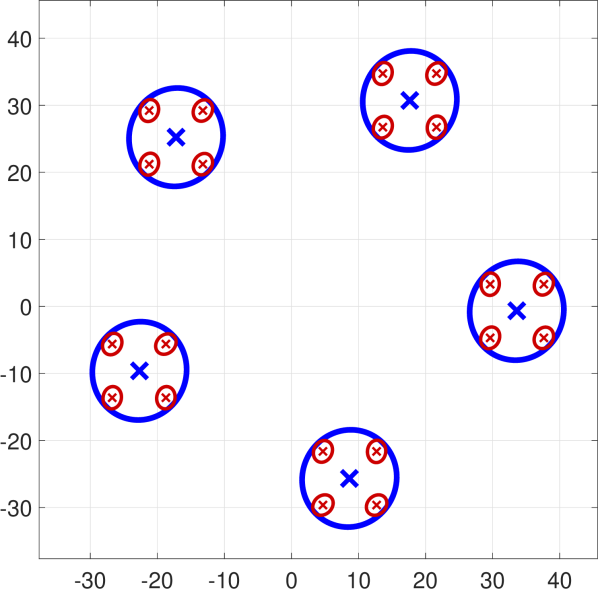
(a)

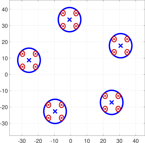
(b)

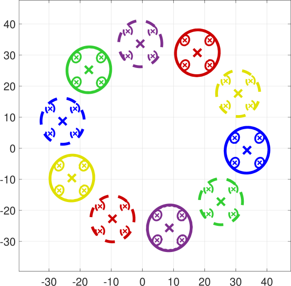
(c)

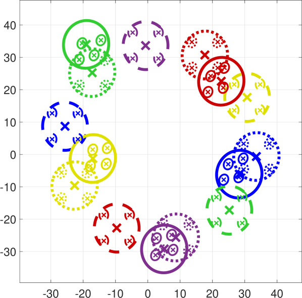
(d)

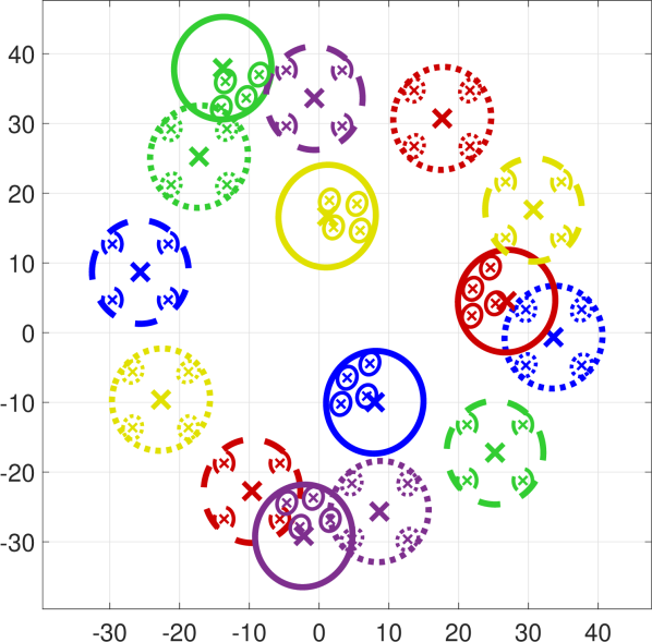
(e)

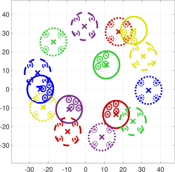
(f)

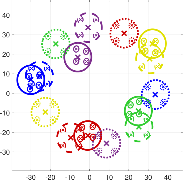
(g)

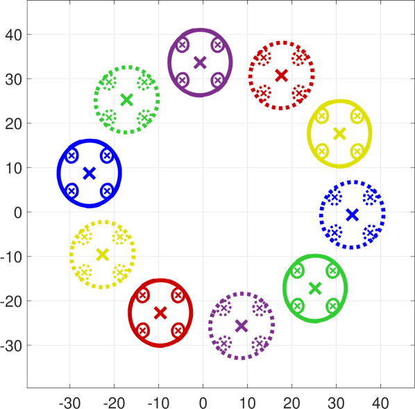
(h)

Figure 3: A two-level small-scale scenario. In (a), the $99.7\%$-confidence ellipses of the initial distributions are shown. Each level corresponds to a specific color (1: blue, 2: red). Similarly, (b) shows the target distributions for the two levels. In (c)-(h), the steering of all distributions is demonstrated for time instants $k=0,20,40,80,80,100$, respectively. At each snapshot, the current, initial and target distributions are shown with solid, dotted and dashed ellipses, respectively. Here, each color corresponds to a specific level-$1$ clique.

Note that as emphasized in Remark 3, we can separate solving (32) into a part that would only involve the variables $\bar{u}_{i}$, $i\in\pazocal{C}_{a}^{\ell-1}$ and a second part including only the variables $L_{i},K_{i}$, $i\in\pazocal{C}_{a}^{\ell-1}$. Let us start with addressing the former part, which can be formulated as

$$\{\bar{u}_{i}\}_{i\in\pazocal{C}_{a}^{\ell-1}}=\operatornamewithlimits{argmin}\sum_{i\in\pazocal{C}_{a}^{\ell-1}}\hat{J}_{i,1}^{\mathrm{s}}(\bar{u}_{i})$$ (35a)

$$\mathrm{s.t.}\quad \mathfrak{f}_{i,N}(\bar{u}_{i})=0,~{}\mathfrak{s}_{i,k}(\bar{u}_{i})\geq 0,~{}\mathfrak{p}_{i,k}(\bar{u}_{i})\leq 0,$$ (35b)

$$\mathfrak{q}_{i,j,k}(\bar{u}_{i},\bar{u}_{j})\geq 0,~{}j\in\mathfrak{n}[\pazocal{C}_{i}^{\ell}],$$ (35c)

$$k\in\llbracket 0,N\rrbracket,~{}i\in\pazocal{C}_{a}^{\ell-1}.$$

where $\hat{J}_{i,1}^{\mathrm{s}}(\bar{u}_{i})=\bar{u}_{i}^{\mathrm{T}}\bar{R}\bar{u}_{i}$. To solve this problem in a distributed manner, we first need to introduce the augmented local variables $\tilde{u}_{i}=[\bar{u}_{i};\{\bar{u}_{j}^{i}\}_{j\in\mathfrak{n}[\pazocal{C}_{i}^{\ell}]}\big{]}$, where $\bar{u}_{j}^{i}$ are copy variables for all $j\in\mathfrak{n}[\pazocal{C}_{i}^{\ell}]$. As in DHDE, we also need to introduce a global variable $b=[\{b_{i}\}_{i\in\pazocal{C}_{a}^{\ell-1}}]$ and the constraints $\tilde{u}_{i}=\tilde{b}_{i}$, where $\tilde{b}_{i}=[b_{i};\{b_{j}\}_{j\in\mathfrak{n}[\pazocal{C}_{i}^{\ell}]}]$. Subsequently, we can arrive to a distributed ADMM algorithm for solving (35). For the full derivation and additional implementation details, the reader is referred to Sections VIII-C and VIII-D of the SM.

The updates of the resulting algorithm are presented below. First, each level-$\ell$ agent updates its local variable $\tilde{u}_{i}$ by solving the following local optimization problem

$$~{}~{}~{}~{}~{}~{}~{}~{}~{}\tilde{u}_{i}=\operatornamewithlimits{argmin}\tilde{J}_{i,1}^{\mathrm{s}}(\bar{u}_{i})$$ (36a)

$$\mathrm{s.t.}\quad \mathfrak{f}_{i,N}(\bar{u}_{i})=0,~{}\mathfrak{s}_{i,k}(\bar{u}_{i})\geq 0,~{}\mathfrak{p}_{i,k}(\bar{u}_{i})\leq 0,$$ (36b)

$$\mathfrak{q}_{i,j,k}(\bar{u}_{i},\bar{u}_{j}^{i})\geq 0,~{}j\in\mathfrak{n}[\pazocal{C}_{i}^{\ell}],~{}k\in\llbracket 0,N\rrbracket.$$ (36c)

with each cost $\tilde{J}_{i,1}^{\mathrm{s}}(\tilde{u}_{i})$ given by

$$\tilde{J}_{i,1}^{\mathrm{s}}(\tilde{u}_{i}) =\hat{J}_{i,1}^{\mathrm{s}}(\bar{u}_{i})+v_{i}^{\mathrm{T}}(\tilde{u}_{i}-\tilde{b}_{i})+\frac{\rho_{u}}{2}\|\tilde{u}_{i}-\tilde{b}_{i}\|_{2}^{2}.$$ (37)

where $\rho_{u}>0$ and $v_{i}$ are the dual variables corresponding to the constraints $\tilde{u}_{i}=\tilde{b}_{i}$. Subsequently, all global variables components are updated with

$$b_{i}\leftarrow\frac{1}{|\mathfrak{m}^{\prime}[\pazocal{C}_{i}^{\ell}]|}\sum_{j\in\mathfrak{m}^{\prime}[\pazocal{C}_{i}^{\ell}]}\bar{u}_{i}^{j}$$ (38)

and, finally, the dual updates are given by

$$v_{i}\leftarrow v_{i}+\rho_{u}(\tilde{u}_{i}-\tilde{b}_{i}).$$ (39)

Again, all updates in (36), (38) and (39) can be performed in parallel by each level-$\ell$ agent $i$. Therefore, all computations are operated in a decentralized fashion. This iterative algorithm repeats until a prespecified termination criterion is met.

Let us now focus on the part of problem (32) that only involves the variables $L_{i},K_{i}$. This subproblem can be formulated as

$$\big{\{}L_{i},K_{i}\big{\}}_{i\in\pazocal{C}_{a}^{\ell-1}}=\operatornamewithlimits{argmin}\sum_{i\in\pazocal{C}_{a}^{\ell-1}}\hat{J}_{i,2}^{\mathrm{s}}(L_{i},K_{i})$$ (40a)

$$\mathrm{s.t.}\quad \pazocal{F}_{i,N}(L_{i},K_{i})\succeq 0,~{}\pazocal{Q}_{i,k}(L_{i},K_{i})\succeq 0,$$ (40b)

$$k\in\llbracket 0,N\rrbracket,~{}i\in\pazocal{C}_{a}^{\ell-1},$$

where $\hat{J}_{i,2}^{\mathrm{s}}(\bar{u}_{i})=\mathrm{tr}(\bar{R}K_{i}WK_{i}^{\mathrm{T}}+\bar{R}L_{i}\Sigma_{i,0}L_{i}^{\mathrm{T}})$. A key observation here is that there exists no inter-agent coupling between the optimization variables of different agents, so we can further split the problem and independently solve each agent’s problem as follows

$$~{}~{}~{}~{}~{}~{}~{}~{}\{L_{i},K_{i}\}=\operatornamewithlimits{argmin}\hat{J}_{i,2}^{\mathrm{s}}(L_{i},K_{i})$$ (41)

$$\mathrm{s.t.}\quad \pazocal{F}_{i,N}(L_{i},K_{i})\succeq 0,~{}\pazocal{Q}_{i,k}(L_{i},K_{i})\succeq 0,~{}k\in\llbracket 0,N\rrbracket.$$

for each $i\in\pazocal{C}_{a}^{\ell-1}$.

The DHDS algorithm with all required computation and communication steps is demonstrated in Alg. 2. The algorithm is executed in a top-down manner for $\ell=\{1,\dots,L\}$. For a specific level $\ell$, each agent $a$ that correspond to a parent clique $\pazocal{C}_{a}^{\ell-1}\in\pazocal{R}^{\ell-1}$ (if $\ell>1$) must send the variables $\mu_{a,k}^{\ell-1},\Sigma_{a,k}^{\ell-1},\ k\in\llbracket 0,N\rrbracket$, to all agents $i\in\pazocal{C}_{a}^{\ell-1}$ (Line 9). Afterwards, the iterative ADMM algorithm starts for every separate group of agents that corresponds to a particular clique $\pazocal{C}_{a}^{\ell-1}$ (Lines 10-18). First, each agent $i\in\pazocal{C}_{a}^{\ell-1}$ solves its local subproblem (36) to update its local variable $\tilde{u}_{i}$ (Line 12). Then, each agent $i$ receives the copy variables $\bar{u}_{i}^{j}$ from all $j\in\mathfrak{m}[\pazocal{C}_{i}^{\ell}]$ (Line 13), so that the variables $b_{i}$ are updated (Line 15) through (38). Subsequently, all agents $j\in\mathfrak{n}[\pazocal{C}_{i}^{\ell}]$ send $b_{j}$ to each $i$ (Line 16) and each agent $i$ updates its dual variable $v_{i}$ (Line 18) with (39). This iterative procedure terminates once a predefined termination criterion is met. Finally, each agent $i\in\pazocal{C}_{a}^{\ell-1}$ also computes its optimal feedback gains $\{L_{i},K_{i}\}$ (Line 20) through solving (41). After the optimal variables $\{\bar{u}_{i},L_{i},K_{i}\}$ have been found for all $i\in\pazocal{C}_{a}^{\ell-1}$, then the state means and covariances $\mu_{i,k}^{\ell},\Sigma_{i,k}^{\ell}$ can be obtained (Line 21) through (31). Subsequently, the same procedure repeats for the next level $\ell+1$, and so on, until level $L$ is reached.

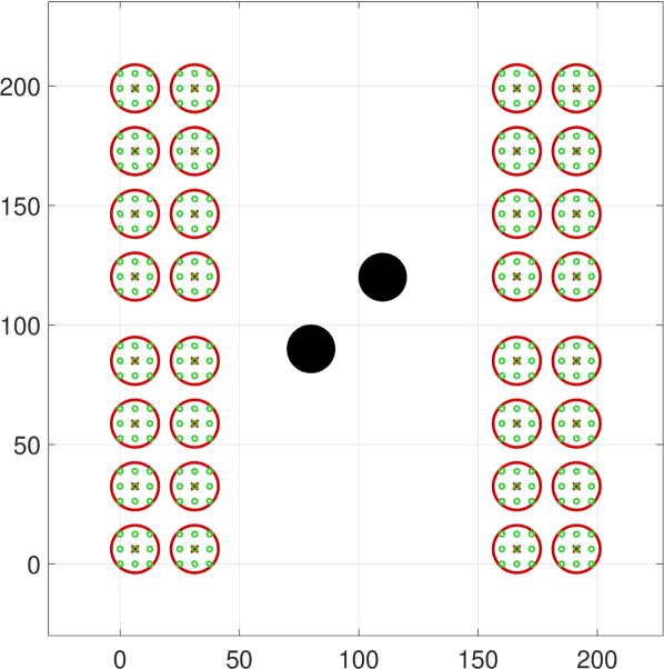
(a)

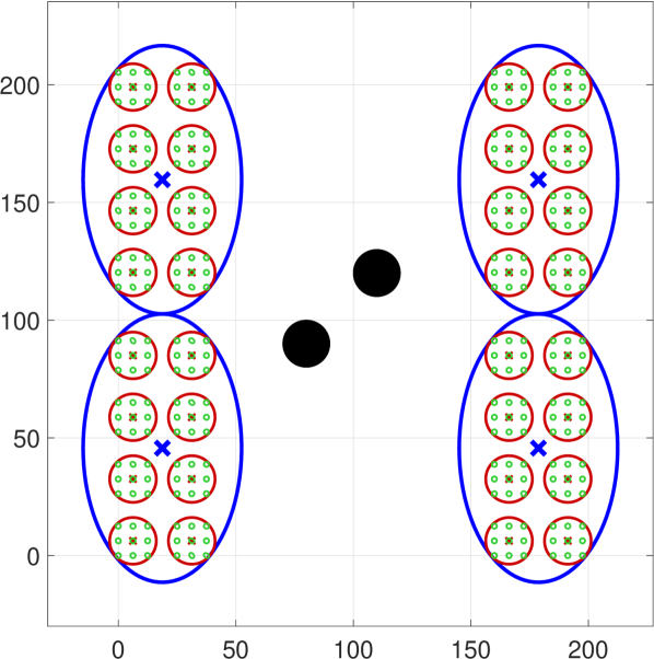
(b)

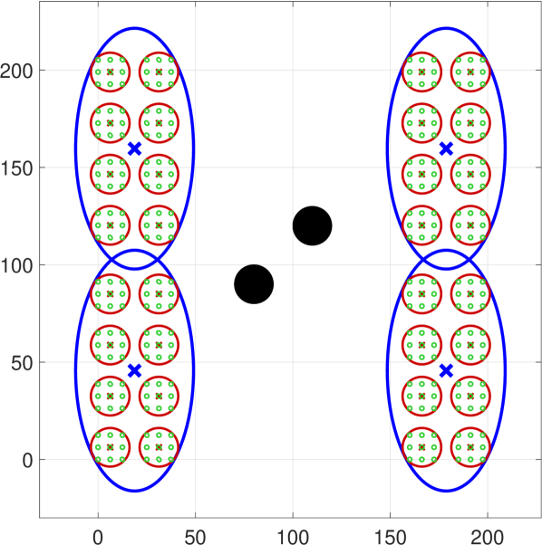
(c)

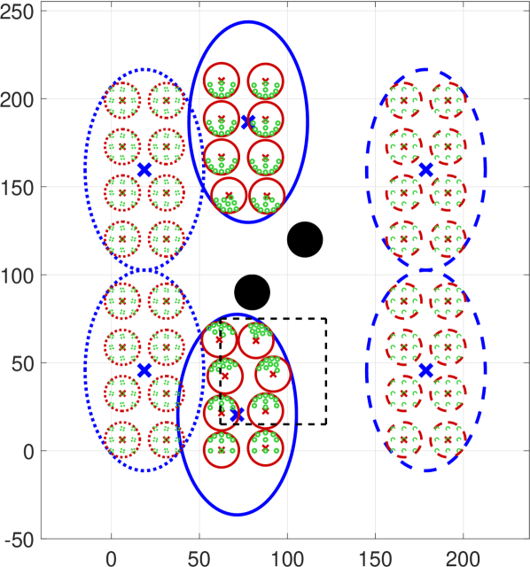
(d)

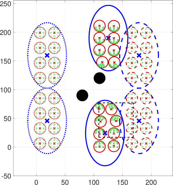
(e)

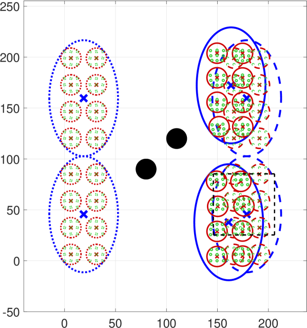
(f)

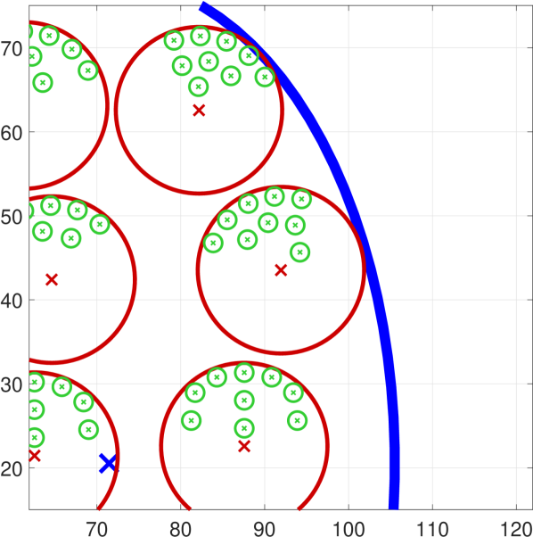
(g)

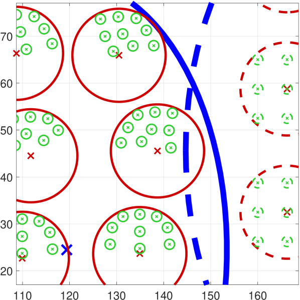
(h)

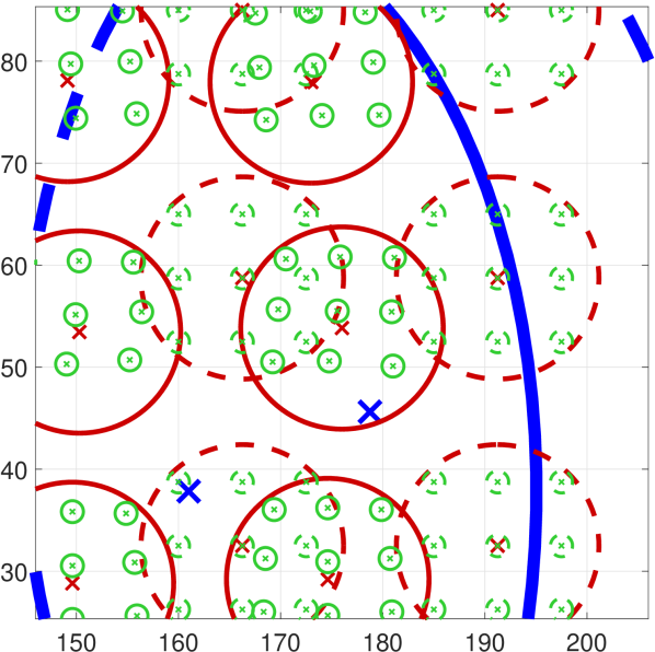
(i)

Figure 4: A three-level large-scale scenario. In (a), the initial (LHS) and target (RHS) distributions of the robots (level $3$, green) are shown along with the level-$2$ ones (red) that are computed by DHDE. In (b), the level-$1$ distributions (blue) that are obtained by DHDE are illustrated. In (c), we show the resulting (overlapping) level-$1$ distributions if the inter-clique non-overlapping constraints are omitted. In (d)-(f), the distributions of all levels are steered to their targets (time instants $k=40,60,80$, respectively), while avoiding the obstacles in the middle (black circles). In (g)-(i), we focus into the black dotted boxes of the above figures and show the motion of the level-$3$ distributions in more detail.

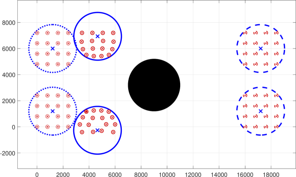
(a)

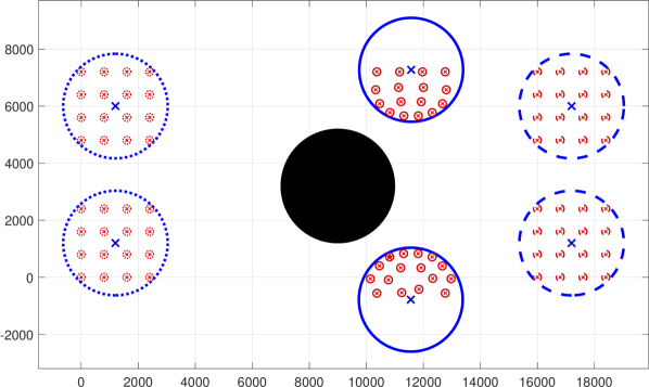
(b)

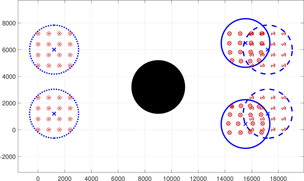
(c)

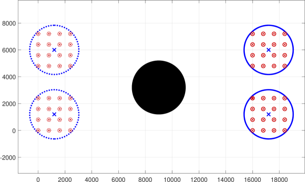
(d)

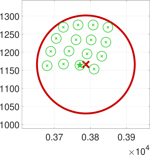
(e)

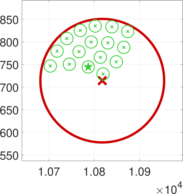
(f)

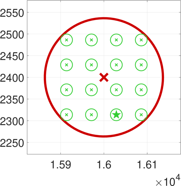
(g)

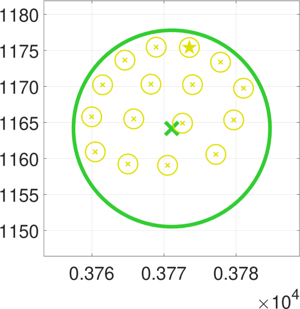
(h)

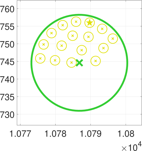
(i)

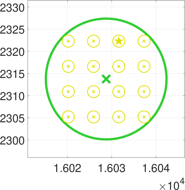
(j)

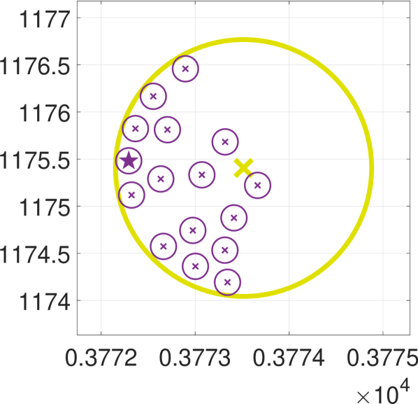
(k)

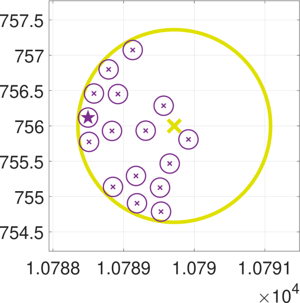
(l)

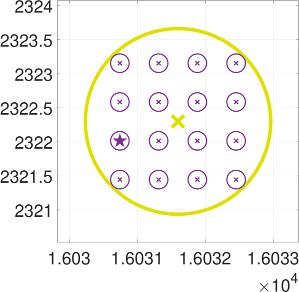
(m)

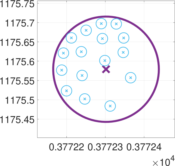
(n)

(o)

(p)

Figure 5: A six-level VLMAS scenario. Each level corresponds to a specific color ($1$: blue, $2$: red, $3$: green, $4$: yellow, $5$: purple, $6$: cyan). Fig. (a)-(d) show levels $1$ and $2$ at time instants $k=30,60,80,100$, respectively. The initial (left) and target (right) distributions are shown with dotted ellipses. Fig. (e)-(g) display one specific level-$2$ clique and its level-$3$ subcliques at $k=30,60,100$. Similarly, Fig. (h)-(j) show one specific level-$3$ clique and its level-$4$ subcliques, Fig. (k)-(m) show one specific level-$4$ clique and its level-$5$ subcliques, and Fig. (n)-(p) show one specific level-$4$ clique and its level-$6$ subcliques, for the same time instants. Each clique we are “zooming“ into, is shown with a star in the figures of the above level.

V Simulation Results

This section provides simulation experiments that verify the effectiveness and scalability of the proposed DHDC framework. In Section V-A, we consider a two-level small-scale system to facilitate the exposition of how DHDE and DHDS operate. A larger three-level system of agents is then used in Section V-B to further illustrate how the two proposed sub-frameworks work. Subsequently, in Section V-C, we showcase the applicability of DHDC on a six-level VLMAS of two million robots. Finally, we compare the proposed approach against other CS methods in Section V-D, and illustrate its superior computational efficiency and safety performance. The reader is encouraged to also refer to the supplementary video for a full illustration of the results.

V-A Small-Scale Scenario

It this task, we consider a two-level small-scale hierarchy with $5$ cliques of $4$ agents, thus a total of $20$ agents (Fig. 3). All agents are modeled with 2D double integrator dynamics. The time horizon of the task is $N=100$. For additional details on the dynamics and algorithmic parameters, the reader is referred to Section IX of the SM. The $99.7\%$-confidence ellipses of the initial Gaussian distributions of the robots are shown in Fig. 3(a) with red color. The level-$1$ distributions that are computed with DHDE also shown with blue color. As expected, the confidence ellipses of the assigned distributions for the level-$1$ cliques encompass the ones of the distributions of the robots (level $2$). Similarly, the target distributions of all levels are illustrated in Fig. 3(b).

The goal of all agents is to reach to a target distribution that is in diametrically opposite position to their initial one, while of course avoiding collisions with the rest of the agents. Figures 3(c)-3(h) show snapshots of the motion of all distributions for time instants $k=0,20,30,40,50,60,70,100$, respectively. As illustrated, DHDS is able to successfully steer all the level-$1$ distributions to the targets provided by DHDE. In the meantime, the distributions of all agents are also steered to their targets while satisfying the constraint that forces their distributions to lie within their parent clique distributions. Thanks to the fact that the solution of the level-$1$ problems guarantees that the agents of one clique will not collide with the ones of other cliques, the level-$2$ subproblems only take into account collision avoidance constraints with agents form the same clique. In Fig. 3(h), all level-$1$ and level-$2$ distributions have successfully reached to their targets.

V-B Large-Scale Scenario

Next, a larger scale $3$-level system of $2\times 8\times 9=144$ agents (Fig. 4) is used to further exhibit the effectiveness of the proposed method. First, we focus on illustrating the performance of the DHDE sub-framework. Figure 4(a) shows the initial and target distributions of the robots (level $3$) and the ones corresponding to the level-$2$ cliques that are obtained through DHDE. In Fig. 4(b), the level-$1$ distributions are shown, while Fig. 4(c) shows the results DHDE would provide if the inter-clique constraints (16c) had been omitted. This highlights the importance of including these constraints and of using the advanced Problem 3 formulation in our setup instead of the more simplistic Problem 2 one.

The performance of the DHDS algorithm is then demonstrated in Figs. 4(d)-4(i). In particular, the motion of the distributions of all levels is shown in Figs. 4(d)-4(f) as they are being steered towards their target while avoiding the obstacles in the middle. In Figs. 4(g)-4(i), we focus into the black dotted box of the previous plots to further emphasize on the motion of the robots (level $3$). As shown, the distributions of the robots are steered while staying within the distributions of their parent cliques and not overlapping with each other.

V-C VLMAS Scenario

Subsequently, we consider a VLMAS with a $6$-level hierarchical clustered structure, where the first level has $2$ cliques, each clique in levels $2,\dots,4$ contains $16$ sub-cliques, and finally each level-$5$ clique contains $16$ agents (level $6$). Therefore, this VLMAS consists of $2\times 16^{5}=2,097,152$ agents. As in the previous tasks, the initial and target distributions of all cliques of all levels are first estimated, and subsequently, the actual distributions are steered while satisfying the probabilistic safety constraints for collision and obstacle avoidance.

Figures 5(a)-5(d) show the distributions of the cliques of levels $1$ and $2$. In particular, the $99.7\%$-confidence regions of the initial (left) and target (right) distributions are shown with dotted ellipses. Note that these distributions are the result of DHDE, first computing the level-$5$ distributions, then the level-$4$ ones, and so on - for a detailed demonstration, the reader is referred to the supplementary video. The motion of all level-$1$ (blue) and level-$2$ (red) distributions is shown in Figs. 5(a)-5(d) for time instants $k=30,60,80,100$. As DHDS is a top-down framework, the level-$1$ distributions are first steered to their targets while successfully avoiding the obstacle. Subsequently, all level-$2$ clique distributions are also steered to their corresponding targets while staying within the limits of their parent cliques and avoiding collisions with each other. In Fig. 5(d) all level-$1,2$ clique distributions have successfully reached to their targets.

In Figs. 5(e)-5(g), we focus into a randomly selected level-$2$ clique and illustrate the motion of the level-$3$ (green) distributions that belong in this clique, for time instants $k=30,60,100$, respectively. As shown, all level-$3$ cliques remain within the limits of their parent cliques, while also avoiding collisions. In Fig. 5(g), the level-3 cliques have reached to their target configuration. Similarly, Figs. 5(h)-5(j) focus into a level-$3$ clique and illustrate the motion of all level-$4$ (yellow) sub-cliques that belong in this clique. Again, all cliques are able to safely reach to their target distributions. The motion of the distributions of specific cliques in levels $5$ (purple) and $6$ (cyan) are also shown in Figs. 5(k)-5(m) and 5(n)-5(p), respectively. All distributions of all levels are successfully steered to their targets, which indicates that all agents have reached their target distributions.

V-D Comparison with Related Methods

Finally, we highlight the significant computational efficiency and safety capabilities of DHDC by comparing it with the Centralized CS (CCS) [4] and Distributed CS (DCS) [31] methods. In CCS, the full level-$L$ CS problem is solved without any splitting being considered. In DCS, the level-$L$ CS problem is solved using an ADMM-based distributed approach, which however cannot benefit from the hierarchical structure of the VLMAS.

V-D1 Computational Demands

To perform a computational demands comparison, we repeat the task of Section V-C, starting from small numbers of agents. All simulations were performed in Matlab R2021b using MOSEK 9.1.9 [1] as the optimization solver and a laptop computer with an 11th Gen Intel(R) Core(TM) i7-11800H @ 2.30GHz and a 32GB RAM memory. The computational times for tasks ranging from two agents to two million agents, are shown in Fig. 6. The results highlight the superior scalability of DHDC against DCS and CCS. This is mainly attributed to the following reasons: i) First, DHDC does not require solving problems of a significantly large scale given that there exist no cliques that contain a very large number of cliques in the level below them. ii) Second, the efficient variables splitting of the subproblems in DHDC reduces the amount of necessary copy variables, making DHDC significantly more computationally efficient than DCS. iii) Third, in CCS, the multi-agent problem is always solved in a centralized fashion, which leads to high-dimensional semidefinite programming problems that soon become computationally intractable.

V-D2 Safety

Next, we conduct a comparison on the safety capabilities of each method. Given that CCS cannot scale for large-scale systems, we exclude it from the comparison. In Fig. 7, we demonstrate the collisions percentages for DHDC and DCS. As both methods enforce consensus through soft constraints, it follows that as tasks get more complicated, collisions might appear. Nevertheless, DHDC outperforms DCS in terms of safety as well, since the cliques/agents always need to only consider safety constraints associated with the other cliques/agents that are within the same clique, thus making the optimization problems easier to solve.

Figure 6: Comparison of computational times between DHDC (proposed), CCS and DCS.

Figure 7: Comparison of collision percentages between DHDC (proposed) and DCS.

VI Conclusion

This paper proposes a scalable hierarchical distributed control framework named DHDC for the control of VLMAS that admit a multi-level hierarchical clustered structure. The first part of the framework, DHDE, associates the initial and target configurations of the cliques of all levels to representative Gaussian distributions that satisfy all the requirements of the hierarchical structure. The second part, DHDS, steers the distributions of all cliques and agents to their prescribed target distributions. Simulation experiments demonstrate the scalability of DHDC to VLMAS with up to two million robots. Therefore, DHDC is shown to be able to control systems of a very-large scale by exploiting the control of distributions within hierarchical structures.

Future work will focus on further expanding DHDC for more general problem setups. A straightforward extension would be to extend the framework for systems nonlinear dynamics by incorporating nonlinear versions of CS [29, 33]. In addition, we wish to extend DHDC for the case where the hierarchical structure is unknown by exploring the incorporation of hierarchical distribution alignment methods in unsupervised learning such as [19, 36]. Finally, future work will also focus on establishing formal convergence guarantees for the proposed method.

Supplementary Material

The following part serves as supplementary material including the proofs and additional details that are not covered in the main paper.

VII DHDE Details

VII-A Proof of Proposition 1

First, it is straightforward to show the equivalence between minimizing the costs in (11a) and (13a), since $\mathbb{D}_{\mathrm{KL}}(\pazocal{N}_{n}^{\ell+1}\|\pazocal{N}_{i}^{\ell})$ is given by

$$\mathbb{D}_{\mathrm{KL}}(\pazocal{N}_{n}^{\ell+1}\|\pazocal{N}_{i}^{\ell})=\frac{1}{2}\bigg{[}\log\frac{|\Sigma_{i}|}{|\Sigma_{n}|}-n_{x}+\mathrm{tr}(\Sigma_{i}^{-1}\Sigma_{n})$$ (42)

$$~{}~{}~{}~{}~{}~{}~{}~{}~{}~{}~{}~{}~{}~{}~{}~{}~{}~{}~{}~{}~{}~{}~{}~{}~{}~{}~{}~{}~{}~{}~{}~{}~{}~{}~{}~{}+(\mu_{i}-\mu_{n})^{\mathrm{T}}\Sigma_{i}^{-1}(\mu_{i}-\mu_{n})\bigg{]}$$

which yields $\hat{J}_{i}^{\mathrm{e}}(Q_{i},q_{i})$ after substituting with $Q_{i}=\Sigma_{i}^{-1}$, $q_{i}=\Sigma_{i}^{-1}\mu_{i}$ and neglecting the constant terms. Note that the objective function $\hat{J}_{i}^{\mathrm{e}}(Q_{i},q_{i})$ is jointly convex for $Q_{i},q_{i}$.

Next, we show the equivalence between the constraints (11b) and (13b)-(13c). For the convenience of the reader, let us first restate a result known as the S-Lemma by Yakubovich [34]. According to the S-Lemma, given two functions $f_{1},f_{2}:\mathbb{R}^{n}\rightarrow\mathbb{R}$ with $f_{1}(x)=x^{\mathrm{T}}A_{1}x+b_{1}^{\mathrm{T}}x+c_{1}$ and $f_{2}(x)=x^{\mathrm{T}}A_{2}x+b_{2}^{\mathrm{T}}x+c_{2}$ and if there exists an $\bar{x}$ such that $f_{1}(\bar{x})>0$, then the following is true

$$f_{1}(x)\geq 0\Rightarrow f_{2}(x)\geq 0,\quad\forall x,$$ (43)

if and only if there exists a $\tau\geq 0$ such that $f_{2}(x)\geq\tau f_{1}(x),\ \forall x$. In constraint (11b), we enforce that if $x\in\mathbb{R}^{n_{p}}$ is such that

$$(x-\bar{\mu}_{n})^{\mathrm{T}}\bar{\Sigma}_{n}^{-1}(x-\bar{\mu}_{n})\leq\alpha,$$ (44)

then it should follow that

$$(x-\bar{\mu}_{i})^{\mathrm{T}}\bar{\Sigma}_{i}^{-1}(x-\bar{\mu}_{i})\leq\alpha.$$ (45)

Using the S-Lemma, this is equivalent with imposing the constraints $\tau_{n}\geq 0,\ \forall n\in\pazocal{C}_{i}^{\ell}$ and

$$\alpha-(x-\bar{\mu}_{i})^{\mathrm{T}}\bar{\Sigma}_{i}^{-1}(x-\bar{\mu}_{i})\geq\tau\big{(}\alpha-(x-\bar{\mu}_{n})^{\mathrm{T}}\bar{\Sigma}_{n}^{-1}(x-\bar{\mu}_{n})\big{)},$$

which can be written in matrix form as

$$\hat{x}^{\mathrm{T}}V_{n}\hat{x}\geq 0,$$ (46)

where $\hat{x}=[x;1]$ and

$$V_{n}=\begin{bmatrix}V_{11}&V_{12}\\ V_{12}^{\mathrm{T}}&V_{22}\end{bmatrix},$$

with

$$V_{11} =-\bar{\Sigma}_{i}^{-1}+\tau_{n}\bar{\Sigma}_{n}^{-1},\ V_{12}=\bar{\Sigma}_{i}^{-1}\bar{\mu}_{i}-\tau_{n}\bar{\Sigma}_{n}^{-1}\bar{\mu}_{n},$$

$$V_{22} =\alpha-\tau_{n}\alpha-\bar{\mu}_{i}^{\mathrm{T}}\bar{\Sigma}_{i}^{-1}\bar{\mu}_{i}+\tau_{n}\bar{\mu}_{n}^{\mathrm{T}}\bar{\Sigma}_{n}^{-1}\bar{\mu}_{n}.$$

By definition, the constraint (46) is equivalent with $V_{n}\succeq 0$. Furthermore, by applying the Schur complement w.r.t. $V_{22}$, it follows that $V_{n}\succeq 0$ is equivalent with $S_{n}\succeq 0$, where

$$S_{n}=\begin{bmatrix}S_{11}&S_{12}&0\\ S_{12}^{\mathrm{T}}&S_{22}&S_{23}\\ 0^{\mathrm{T}}&S_{23}^{\mathrm{T}}&S_{33}\end{bmatrix},$$ (47)

with

$$S_{11} =V_{11},\ S_{12}=V_{12},\ S_{22}=\alpha-\tau_{n}\alpha+\tau_{n}\bar{\mu}_{n}^{\mathrm{T}}\bar{\Sigma}_{n}^{-1}\bar{\mu}_{n},$$

$$\ S_{23} =(\bar{\Sigma}_{i}^{-1}\bar{\mu}_{i})^{\mathrm{T}},\ S_{33}=\bar{\Sigma}_{i}^{-1}.$$

The expressions in (14c) follow after substituting with $Q_{i}$ and $q_{i}$. Finally, it is evident that the constraints (11c) and (13d) are equivalent since $\Sigma_{i}\succ 0$ if and only if $\Sigma_{i}^{-1}\succ 0$. Note that all constraints are convex as well. Therefore, the problem presented in Proposition 1 is a convex optimization one.

VII-B Proof of Proposition 2

The equivalence between the costs (16a) and (17a), as well as the equivalence between the constraints (16b) and (17b)-(17c) follow directly from Proposition 1. Next, we show that if the constraints (17d) and (17e) are satisfied, then the constraint (16c) is also satisfied. In fact, the constraint

$$\pazocal{E}_{\theta}[\bar{\mu}_{i},\bar{\Sigma}_{i}]\cap\pazocal{E}_{\theta}[\bar{\mu}_{j},\bar{\Sigma}_{j}]=\emptyset$$ (48)

will hold if the following constraint holds

$$\mathscr{C}\big{[}\pazocal{E}_{\theta}[\bar{\mu}_{i},\bar{\Sigma}_{i}]\big{]}\cap\mathscr{C}\big{[}\pazocal{E}_{\theta}[\bar{\mu}_{j},\bar{\Sigma}_{j}]\big{]}=\emptyset,$$ (49)

where $\mathscr{C}[\pazocal{E}]$ denotes the minimum area enclosing circle of an ellipse $\pazocal{E}$. Of course, $\mathscr{C}\big{[}\pazocal{E}_{\theta}[\bar{\mu}_{i},\bar{\Sigma}_{i}]\big{]}$ is a circle with center $\bar{\mu}_{i}$ and radius $\sqrt{\alpha\lambda_{\max}(\bar{\Sigma}_{i})}$, which is the major axis length of $\pazocal{E}_{\theta}[\bar{\mu}_{i},\bar{\Sigma}_{i}]$. Hence, the constraint (49) can be rewritten as

$$\|\bar{\mu}_{i}-\bar{\mu}_{j}\|_{2}\geq\sqrt{\alpha\lambda_{\max}(\bar{\Sigma}_{i})}+\sqrt{\alpha\lambda_{\max}(\bar{\Sigma}_{j})}.$$ (50)

or equivalently as

$$\|\bar{Q}_{i}^{-1}\bar{q}_{i}-\bar{Q}_{j}^{-1}\bar{q}_{j}\|_{2}\geq\frac{\sqrt{\alpha}}{\sqrt{\lambda_{\min}(\bar{Q}_{i})}}+\frac{\sqrt{\alpha}}{\sqrt{\lambda_{\min}(\bar{Q}_{j})}}.$$ (51)

By introducing the auxiliary variables $\phi_{i},\phi_{j}$, the constraint (51) is equivalent with the set of constraints

$$\|\bar{Q}_{i}^{-1}\bar{q}_{i}-\bar{Q}_{j}^{-1}\bar{q}_{j}\|_{2}\geq\phi_{i}^{-1/2}+\phi_{j}^{-1/2},$$ (52a)

$$\phi_{l}^{-1/2}\geq\frac{\sqrt{\alpha}}{\sqrt{\lambda_{\min}(\bar{Q}_{l})}},\ l\in\{i,j\}$$ (52b)

where (52a) is the same as (17d). The constraint (52b) can be rewritten as

$$\bar{Q}_{l}\succeq\phi_{l}\alpha I$$ (53)

which yields (17e). Finally, the constraints (16d) and (17f) are equivalent.

VII-C ADMM Derivation

After introducing the augmented variables $\tilde{Q}_{i}$, $\tilde{q}_{i}$, $\tilde{\phi}_{i}$, and the global ones $G$, $g$, $z$, the problem presented in Proposition 2 can be reformulated as

$$~{}~{}~{}~{}~{}~{}\min\sum_{i\in\pazocal{C}_{a}^{\ell-1}}\hat{J}_{i}^{\mathrm{e}}(Q_{i},q_{i})$$ (54a)

$$\mathrm{s.t}\quad S_{i,n}(Q_{i},q_{i},\tau_{i,n})\succeq 0,\ n\in\pazocal{C}_{i}^{\ell},$$ (54b)

$$\tau_{i,n}\geq 0,\ n\in\pazocal{C}_{i}^{\ell},$$ (54c)

$$h_{i}(\tilde{Q}_{i},\tilde{q}_{i},\tilde{\phi}_{i})\leq 0,$$ (54d)

$$T_{i}(Q_{i},\phi_{i})\succeq 0,$$ (54e)

$$Q_{i}\succeq 0,$$ (54f)

$$\tilde{Q}_{i}=\tilde{G}_{i},\ \tilde{q}_{i}=\tilde{g}_{i},\ \tilde{\phi}_{i}=\tilde{z}_{i},\ i\in\pazocal{C}_{a}^{\ell-1},$$ (54g)

where $h_{i}(\tilde{Q}_{i},\tilde{q}_{i},\tilde{\phi}_{i})$ is defined as

$$h_{i}=[\{h_{i,j}(Q_{i},q_{i},\phi_{i},Q_{j}^{i},q_{j}^{i},\phi_{j}^{i})\}_{j\in\mathfrak{n}[\pazocal{C}_{i}^{\ell}]}].$$ (55)

Let us also introduce the indicator functions $\pazocal{I}_{S_{i}}(Q_{i},q_{i},\tau_{i,n})$, $\pazocal{I}_{\tau_{i,n}}(\tau_{i,n})$, $\pazocal{I}_{h_{i}}(\tilde{Q}_{i},\tilde{q}_{i},\tilde{\phi}_{i})$, $\pazocal{I}_{T_{i}}(Q_{i},\phi_{i})$, $\pazocal{I}_{Q_{i}}(Q_{i})$, which take a zero value if the constraints (54b), (54c), (54d), (54e), (54f), respectively, are satisfied, and become infinite, otherwise. Then, the Augmented Lagrangian (AL) for this problem can be formulated as

$$\pazocal{L} =\sum_{i\in\pazocal{C}_{a}^{\ell-1}}\hat{J}_{i}^{\mathrm{e}}(Q_{i},q_{i})+\pazocal{I}_{h_{i}}(\tilde{Q}_{i},\tilde{q}_{i},\tilde{\phi}_{i})+\pazocal{I}_{T_{i}}(Q_{i},\phi_{i})$$

$$~{}~{}~{}~{}~{}~{}~{}~{}~{}+\pazocal{I}_{Q_{i}}(Q_{i})+\sum_{n\in\pazocal{C}_{i}^{\ell}}\pazocal{I}_{S_{i,n}}(Q_{i},q_{i},\tau_{i,n})+\pazocal{I}_{\tau_{i,n}}(\tau_{i,n})$$

$$~{}~{}~{}~{}~{}~{}~{}~{}~{}+\mathrm{tr}(\Xi_{i}^{\mathrm{T}}(\tilde{Q}_{i}-\tilde{G}_{i}))+\xi_{i}^{\mathrm{T}}(\tilde{q}_{i}-\tilde{g}_{i})+y_{i}^{\mathrm{T}}(\tilde{\phi}_{i}-\tilde{z}_{i})$$

$$~{}~{}~{}~{}~{}~{}~{}~{}~{}+\frac{\rho_{Q}}{2}\|\tilde{Q}_{i}-\tilde{G}_{i}\|_{F}^{2}+\frac{\rho_{q}}{2}\|\tilde{q}_{i}-\tilde{g}_{i}\|_{2}^{2}+\frac{\rho_{\phi}}{2}\|\tilde{\phi}_{i}-\tilde{z}_{i}\|_{2}^{2}.$$

Therefore, the ADMM updates are derived as follows. First, the updates for the variables $\tilde{Q}_{i}$, $\tilde{q}_{i}$ and $\tilde{\phi}_{i}$, are given by

$$\{\tilde{Q}_{i},\tilde{q}_{i},\tilde{\phi}_{i}\}=\operatornamewithlimits{argmin}\pazocal{L}$$ (56)

for all $i\in\pazocal{C}_{a}^{\ell-1}$. The minimization in (56) leads to the local problems

$$\{\tilde{Q}_{i},\tilde{q}_{i},\tilde{\phi}_{i}\}=\operatornamewithlimits{argmin}\tilde{J}_{i}^{\mathrm{e}}(\tilde{Q}_{i},\tilde{q}_{i},\tilde{\phi}_{i})$$ (57a)

$$\mathrm{s.t}\quad S_{i,n}(Q_{i},q_{i},\tau_{i,n})\succeq 0,\ n\in\pazocal{C}_{i}^{\ell},$$ (57b)

$$\tau_{i,n}\geq 0,\ n\in\pazocal{C}_{i}^{\ell},$$ (57c)

$$h_{i}(\tilde{Q}_{i},\tilde{q}_{i},\tilde{\phi}_{i})\leq 0,$$ (57d)

$$T_{i}(Q_{i},\phi_{i})\succeq 0,$$ (57e)

$$Q_{i}\succ 0,$$ (57f)

where

$$\tilde{J}_{i}^{\mathrm{e}} =\hat{J}_{i}^{\mathrm{e}}(Q_{i},q_{i})+\mathrm{tr}(\Xi_{i}^{\mathrm{T}}(\tilde{Q}_{i}-\tilde{G}_{i}))+\xi_{i}^{\mathrm{T}}(\tilde{q}_{i}-\tilde{g}_{i})$$

$$~{}~{}+y_{i}^{\mathrm{T}}(\tilde{\phi}_{i}-\tilde{z}_{i})+\frac{\rho_{Q}}{2}\|\tilde{Q}_{i}-\tilde{G}_{i}\|_{F}^{2}+\frac{\rho_{q}}{2}\|\tilde{q}_{i}-\tilde{g}_{i}\|_{2}^{2}$$

$$~{}~{}+\frac{\rho_{\phi}}{2}\|\tilde{\phi}_{i}-\tilde{z}_{i}\|_{2}^{2}.$$ (58)

Subsequently, the global variables $G$, $g$ and $z$ are updated by

$$\{G,g,z\}=\operatornamewithlimits{argmin}\pazocal{L}.$$ (59)

using the updated values of $\tilde{Q}_{i}$, $\tilde{q}_{i}$ and $\tilde{\phi}_{i}$, $\forall i\in\pazocal{C}_{a}^{\ell-1}$. The minimization in (59) can be separated for all $G_{i}$, $g_{i}$ and $z_{i}$, leading to the following averaging steps

$$G_{i} =\frac{1}{|\mathfrak{m}^{\prime}[\pazocal{C}_{i}^{\ell}]|}\sum_{j\in\mathfrak{m}^{\prime}[\pazocal{C}_{i}^{\ell}]}Q_{i}^{j}$$ (60a)

$$g_{i} =\frac{1}{|\mathfrak{m}^{\prime}[\pazocal{C}_{i}^{\ell}]|}\sum_{j\in\mathfrak{m}^{\prime}[\pazocal{C}_{i}^{\ell}]}q_{i}^{j}$$ (60b)

$$z_{i} =\frac{1}{|\mathfrak{m}^{\prime}[\pazocal{C}_{i}^{\ell}]|}\sum_{j\in\mathfrak{m}^{\prime}[\pazocal{C}_{i}^{\ell}]}\phi_{i}^{j}.$$ (60c)

After these updates are performed, then the dual variables are updated through dual ascent steps, as follows

$$\Xi_{i} \leftarrow\Xi_{i}+\rho_{Q}(\tilde{Q}_{i}-\tilde{G}_{i})$$ (61a)

$$\xi_{i} \leftarrow\xi_{i}+\rho_{q}(\tilde{q}_{i}-\tilde{g}_{i})$$ (61b)

$$y_{i} \leftarrow y_{i}+\rho_{\phi}(\tilde{\phi}_{i}-\tilde{z}_{i}),$$ (61c)

by all $i\in\pazocal{C}_{a}^{\ell-1}$.

VII-D Implementation Details

VII-D1 Constraint Linearization

In the local problems (21), all cost terms and constraints are convex, except for the constraint (21d). We accommodate for that by linearizing the constraint in every ADMM iteration around the previous values of the included variables, which we denote with $\bar{Q}_{i}^{\prime},\bar{q}_{i}^{\prime},\phi_{i}^{\prime},\bar{Q}_{j}{}^{\prime},\bar{q}_{j}{}^{\prime},\phi_{j}{}^{\prime}$, where we drop the superscript $i$ to lighten the notation. The first order Taylor approximation of $h_{i,j}$ around $(\bar{Q}_{i}^{\prime},\bar{q}_{i}^{\prime},\phi_{i}^{\prime},\bar{Q}_{j}{}^{\prime},\bar{q}_{j}{}^{\prime},\phi_{j}{}^{\prime})$ is denoted by $\bar{h}_{i,j}(\bar{Q}_{i},\bar{q}_{i},\phi_{i},\bar{Q}_{j},\bar{q}_{j},\phi_{j})$ where

$$\bar{h}_{i,j} =h_{i,j}(\bar{Q}_{i}^{\prime},\bar{q}_{i}^{\prime},\phi_{i}^{\prime},\bar{Q}_{j}^{\prime},\bar{q}_{j}^{\prime},\phi_{j}^{\prime})+\mathrm{tr}\left(\nabla_{\bar{Q}_{i}}h_{i,j}\Bigr{\rvert}_{\bar{Q}_{i}^{\prime}}^{\mathrm{T}}(\bar{Q}_{i}-\bar{Q}_{i}^{\prime})\right)$$

$$~{}~{}~{}~{}+\mathrm{tr}\left(\nabla_{\bar{Q}_{j}}h_{i,j}\Bigr{\rvert}_{\bar{Q}_{j}^{\prime}}^{\mathrm{T}}(\bar{Q}_{j}-\bar{Q}_{j}^{\prime})\right)+\nabla_{\bar{q}_{i}}h_{i,j}\Bigr{\rvert}_{\bar{q}_{i}^{\prime}}^{\mathrm{T}}(\bar{q}_{i}-\bar{q}_{i}^{\prime})$$

$$~{}~{}~{}~{}+\nabla_{\bar{q}_{j}}h_{i,j}\Bigr{\rvert}_{\bar{q}_{j}^{\prime}}^{\mathrm{T}}(\bar{q}_{j}-\bar{q}_{j}^{\prime})+\frac{\partial h_{i,j}}{\partial\phi_{j}}\biggr{\rvert}_{\phi_{j}^{\prime}}(\phi_{j}-\phi_{j}^{\prime})$$

$$~{}~{}~{}~{}+\frac{\partial h_{i,j}}{\partial\phi_{i}}\biggr{\rvert}_{\phi_{i}^{\prime}}(\phi_{i}-\phi_{i}^{\prime}),$$

with

$$\nabla_{\bar{Q}_{i}}h_{i,j} =\frac{1}{\|\omega_{i,j}\|_{2}}\bar{Q}_{i}^{-\mathrm{T}}\omega_{i,j}(\bar{Q}_{i}^{-1}\bar{q}_{i})^{\mathrm{T}}$$

$$\nabla_{\bar{Q}_{j}}h_{i,j} =-\frac{1}{\|\omega_{i,j}\|_{2}}\bar{Q}_{j}^{-\mathrm{T}}\omega_{i,j}(\bar{Q}_{j}^{-1}\bar{q}_{j})^{\mathrm{T}}$$

$$\nabla_{\bar{q}_{i}}h_{i,j} =-\frac{1}{\|\omega_{i,j}\|_{2}}\bar{Q}_{i}^{-\mathrm{T}}\omega_{i,j}$$

$$\nabla_{\bar{q}_{j}}h_{i,j} =\frac{1}{\|\omega_{i,j}\|_{2}}\bar{Q}_{j}^{-\mathrm{T}}\omega_{i,j}$$

$$\omega_{i,j} =\bar{Q}_{i}^{-1}\bar{q}_{i}-\bar{Q}_{j}^{-1}\bar{q}_{j},$$

$$\frac{\partial h_{i,j}}{\partial\phi_{i}} =-\frac{1}{2}\phi_{i}^{-3/2},\quad\frac{\partial h_{i,j}}{\partial\phi_{j}}=-\frac{1}{2}\phi_{j}^{-3/2}.$$

VII-D2 Termination Criterion

We suggest two options for the termination criterion in Line 10 of Alg. 1. The first one that would not require any additional communication would be to just set a maximum amount of ADMM iterations. The second option would be to also check whether the ADMM primal and dual residuals norms are below some prespecified thresholds to allow for early termination. In particular, the primal residuals norms are given by

$$\epsilon_{\mathrm{primal},1} =\sum_{i\in\pazocal{C}_{a}^{\ell-1}}\|\tilde{Q}_{i}-\tilde{T}_{i}\|_{F},$$

$$\epsilon_{\mathrm{primal},2} =\sum_{i\in\pazocal{C}_{a}^{\ell-1}}\|\tilde{q}_{i}-\tilde{t}_{i}\|_{2},$$

$$\epsilon_{\mathrm{primal},3} =\sum_{i\in\pazocal{C}_{a}^{\ell-1}}\|\tilde{\phi}_{i}-\tilde{z}_{i}\|_{2},$$

while the dual residuals norms are given by

$$\epsilon_{\mathrm{dual},1} =\rho_{Q}\sum_{i\in\pazocal{C}_{a}^{\ell-1}}\|\tilde{T}_{i}-\tilde{T}_{i,\mathrm{prev}}\|_{F},$$

$$\epsilon_{\mathrm{dual},2} =\rho_{q}\sum_{i\in\pazocal{C}_{a}^{\ell-1}}\|\tilde{t}_{i}-\tilde{t}_{i,\mathrm{prev}}\|_{2},$$

$$\epsilon_{\mathrm{dual},3} =\rho_{\phi}\sum_{i\in\pazocal{C}_{a}^{\ell-1}}\|\tilde{z}_{i}-\tilde{z}_{i,\mathrm{prev}}\|_{2}.$$

Note that the latter approach would require all agents $i\in\pazocal{C}_{a}^{\ell-1}$ sending their variables to agent $a$ so that the residuals are computed.

VIII DHDS Details

VIII-A Detailed Expressions

The decision variables $\bar{u}_{i}\in\mathbb{R}^{Nn_{u}}$, $L_{i}\in\mathbb{R}^{Nn_{u}\times n_{x}}$ and $K_{i}\in\mathbb{R}^{Nn_{u}\times Nn_{x}}$ are given by $\bar{u}_{i}=[\bar{u}_{i,0};\dots;\bar{u}_{i,N-1}]$,

$$~{}~{}~{}~{}~{}~{}~{}~{}~{}~{}~{}~{}\bar{u}_{i}=\begin{bmatrix}\bar{u}_{i,0}^{\mathrm{T}}&\bar{u}_{i,1}^{\mathrm{T}}&\cdots&\bar{u}_{i,N-1}^{\mathrm{T}}\end{bmatrix}^{\mathrm{T}},$$

$$~{}~{}~{}~{}~{}~{}~{}~{}~{}~{}~{}~{}L_{i}=\begin{bmatrix}L_{i,0}^{\mathrm{T}}&L_{i,1}^{\mathrm{T}}&\cdots&L_{i,N-1}^{\mathrm{T}}\end{bmatrix}^{\mathrm{T}},$$

$$K_{i} =\begin{bmatrix}0&0&\dots&0&0\\ K_{i,(0,0)}&0&\dots&0&0\\ K_{i,(1,0)}&K_{i,(1,1)}&\dots&0&0\\ \vdots&\vdots&\ddots&\vdots&\vdots\\ K_{i,(N-2,0)}&K_{i,(N-2,1)}&\dots&K_{i,(N-2,N-2)}&0\end{bmatrix}.$$

The matrices $\Psi_{0}$, $\Psi_{u}$ and $\Psi_{w}$ have the following form

$$\Psi_{0}=\begin{bmatrix}I&A^{\mathrm{T}}&\cdots&A^{N}{}^{\mathrm{T}}\end{bmatrix}^{\mathrm{T}},$$

$$\Psi_{u}=\begin{bmatrix}0&0&\dots&0\\ B&0&\cdots&0\\ AB&B&\cdots&0\\ \vdots&\vdots&\ddots&\vdots\\ A^{N-1}B&A^{N-2}B&\cdots&B\end{bmatrix},$$

$$\Psi_{w}=\begin{bmatrix}0&0&\dots&0\\ I&0&\cdots&0\\ A&I&\cdots&0\\ \vdots&\vdots&\ddots&\vdots\\ A^{N-1}&A^{N-2}&\cdots&I\end{bmatrix}.$$

The mean state $\mu_{i,k}$ is given by

$$\mu_{i,k}=f_{i,k}(\bar{u}_{i})=P_{k}f_{i}(\bar{u}_{i}),$$ (62)

where

$$f_{i}(\bar{u}_{i})=\Psi_{0}\mu_{i,0}+\Psi_{u}\bar{u}_{i},$$ (63)

and $P_{k}:=\begin{bmatrix}0,\dots,I,\dots,0\end{bmatrix}\in\mathbb{R}^{N_{x}\times(N+1)N_{x}}$. Furthermore, the state covariance $\Sigma_{i,k}$ is given by

$$\Sigma_{i,k}=F_{i,k}(L_{i},K_{i})=P_{k}F_{i}(L_{i},K_{i})P_{k}^{\mathrm{T}},$$ (64)

where

$$F_{i}(L_{i},K_{i}) :=(\Psi_{0}+\Psi_{u}L_{i})\Sigma_{i,0}(\Psi_{0}+\Psi_{u}L_{i})^{\mathrm{T}}$$

$$~{}~{}~{}~{}+(\Psi_{w}+\Psi_{u}K_{i})\bar{W}(\Psi_{w}+\Psi_{u}K_{i})^{\mathrm{T}}.$$

with $\bar{W}=\mathrm{blkdiag}(W,\dots,W)\in\mathbb{S}_{Nn_{x}}^{+}$.

VIII-B Proof of Proposition 3

First, let us show the equivalence between costs (25a) and (32a). The cost function $J_{i}^{\mathrm{s}}(u_{i}^{\ell})$ can be rewritten as

$$J_{i}^{\mathrm{s}}(u_{i}) =\mathbb{E}[u_{i}^{\mathrm{T}}\bar{R}u_{i}]=\mathbb{E}\big{[}\mathrm{tr}(\bar{R}_{i}u_{i}u_{i}^{\mathrm{T}})\big{]}=\mathrm{tr}\big{(}\mathbb{E}[\bar{R}_{i}u_{i}u_{i}^{\mathrm{T}}]\big{)}.$$

Using (28), we obtain

$$J_{i}^{\mathrm{s}}(u_{i}) =\hat{J}_{i}^{\mathrm{s}}(\bar{u}_{i},L_{i},K_{i})$$

$$=\mathrm{tr}\big{(}\mathbb{E}[\bar{R}_{i}(\bar{u}_{i}+L_{i}\tilde{x}_{i,0}+K_{i}w_{i})(\bar{u}_{i}+L_{i}\tilde{x}_{i,0}+K_{i}w_{i})^{\mathrm{T}}]\big{)}$$

$$=\mathrm{tr}(\bar{R}\bar{u}_{i}\bar{u}_{i}^{\mathrm{T}}+\bar{R}K_{i}WK_{i}^{\mathrm{T}}+\bar{R}L_{i}\Sigma_{i,0}L_{i}^{\mathrm{T}})$$

$$=\bar{u}_{i}^{\mathrm{T}}\bar{R}\bar{u}_{i}+\mathrm{tr}(\bar{R}K_{i}WK_{i}^{\mathrm{T}}+\bar{R}L_{i}\Sigma_{i,0}L_{i}^{\mathrm{T}}),$$

where $\tilde{x}_{i,0}=x_{i,0}-\mu_{i,0}$ and we used the facts that $\mathbb{E}[\tilde{x}_{i,0}]=0$, $\mathbb{E}[\tilde{x}_{i,0}w_{i}^{\mathrm{T}}]=0$, $\mathbb{E}[w_{i}w_{i}^{\mathrm{T}}]=\bar{W}$ and $\mathbb{E}[\tilde{x}_{i,0}\tilde{x}_{i,0}^{\mathrm{T}}]=\Sigma_{i,0}$. Furthermore, the dynamics constraints (25b) are implicitly satisfied since in all expressions we use (31) for the state means and covariances.

It is also trivial to show that the constraint $\mathfrak{f}_{i,N}(\bar{u}_{i})=0$ is equivalent to $\mathbb{E}[x_{i,N}]=\mu_{i,\mathrm{f}}$. Moreover, if we write $F_{i}(L_{i},K_{i})=\Phi_{i}(L_{i},K_{i})\Phi_{i}(L_{i},K_{i})^{\mathrm{T}}$ with

$$\Phi_{i}(L_{i},K_{i})=\begin{bmatrix}(\Psi_{0}+\Psi_{u}L_{i})&(\Psi_{w}+\Psi_{u}K_{i})\end{bmatrix}\Omega_{i},$$ (65)

where $\Omega_{i}\Omega_{i}^{\mathrm{T}}=\mathrm{blkdiag}(\Sigma_{i,0},W)$ and define $\Phi_{i,k}(L_{i},K_{i})=P_{k}\Phi_{i}(L_{i},K_{i})$, then the constraint $\Sigma_{i,\mathrm{f}}\succeq F_{i,N}(L_{i},K_{i})=\Phi_{i,k}(L_{i},K_{i})\Phi_{i,k}(L_{i},K_{i})^{\mathrm{T}}$ is equivalent with

$$\pazocal{F}_{i,N}(L_{i},K_{i})=\begin{bmatrix}\Sigma_{i,\mathrm{f}}&\Phi_{i,N}(L_{i},K_{i})\\ \Phi_{i,N}(L_{i},K_{i})^{\mathrm{T}}&I\end{bmatrix}\succeq 0$$ (66)

by using the Schur complement of $\pazocal{F}_{i,N}(L_{i},K_{i})$ w.r.t. $I$.

Subsequently, we show that if the constraints $\pazocal{Q}_{i,k}(L_{i},K_{i})\succeq 0$ and $\mathfrak{q}_{i,j,k}(\bar{u}_{i},\bar{u}_{j})\geq 0$ are satisfied, then the constraint $q_{i,j,k}(p_{i,k},p_{j,k})\geq 0$ is satisfied as well. In particular, the latter constraint will be true if the following inequalities hold,

$$\|\bar{\mu}_{i,k}-\bar{\mu}_{j,k}\|_{2}\geq d_{\mathrm{inter}}+2r,$$ (67a)

$$~{}~{}~{}~{}~{}\sqrt{\alpha\lambda_{\mathrm{max}}(\bar{\Sigma}_{i,k})}\leq r,$$ (67b)

where we drop the superscripts $\ell$ for notational convenience. If we plug the mean state expressions into (67a), then we obtain

$$\|\bar{f}_{i,k}(\bar{u}_{i})-\bar{f}_{j,k}(\bar{u}_{j})\|_{2}\geq d_{\mathrm{inter}}+2r,$$ (68)

which yields the constraint $\mathfrak{q}_{i,j,k}(\bar{u}_{i},\bar{u}_{j})\geq 0$. Furthermore, the constraint (67b) can be rewritten as

$$\lambda_{\mathrm{max}}(\bar{\Sigma}_{i,k})\leq\frac{r^{2}}{\alpha}.$$ (69)

which is equivalent with

$$HF_{i,k}(L_{i},K_{i})H^{\mathrm{T}}-\frac{r^{2}}{\alpha}\preceq 0.$$ (70)

or using again the Schur complement with

$$\begin{bmatrix}\big{(}\frac{r^{\ell}}{\sqrt{\alpha}}\big{)}^{2}I&H\Phi_{i,k}(L_{i},K_{i})\\ \Phi_{i,k}(L_{i},K_{i})^{\mathrm{T}}H^{\mathrm{T}}&I\end{bmatrix}\succeq 0$$ (71)

which is identical with $\pazocal{Q}_{i,k}(L_{i},K_{i})\succeq 0$. With similar arguments, it can be shown that if the constraints $\pazocal{Q}_{i,k}(L_{i},K_{i})\succeq 0$ and $\mathfrak{s}_{i,k}(\bar{u}_{i})\geq 0$ are satisfied, then the constraint $s_{i,k}(p_{i.k})\geq 0$ is also satisfied.

Finally, we wish to show that if the constraint $\mathfrak{p}(\bar{u}_{i})\leq 0$ is true, then the constraint (25f) is also true. Since (67b) holds, then it suffices to enforce a contraint that $\bar{\mu}_{i,k}^{\ell}$ should lie within an ellipse with center $\bar{\mu}_{a,k}^{(\ell-1)}$, major axis length $\sqrt{\alpha\lambda_{\mathrm{max}}(\bar{\Sigma}_{a,k}^{(\ell-1)})}-r$, minor axis length $\sqrt{\alpha\lambda_{\mathrm{min}}(\bar{\Sigma}_{a,k}^{(\ell-1)})}-r$, and the same orientation as the ellipse $\pazocal{E}_{\theta}[\bar{\mu}_{a,k}^{\ell-1},\bar{\Sigma}_{a,k}^{\ell-1}]$. These specifications can be captured if the following inequality holds

$$(\bar{\mu}_{i,k}^{\ell}-\bar{\mu}_{a,k}^{\ell-1})^{\mathrm{T}}\hat{P}(\bar{\mu}_{i,k}^{\ell}-\bar{\mu}_{a,k}^{\ell-1})\leq 1,$$ (72)

where

$$~{}~{}~{}\hat{P}=\frac{1}{\alpha}U\hat{\Lambda}^{-1}U^{\mathrm{T}},$$

$$\hat{\Lambda}=\left(\Lambda^{1/2}-\frac{r}{\sqrt{\alpha}}I\right)^{2},$$

and $[\Lambda,U]$ is the eigendecomposition of $\bar{\Sigma}_{a,k}^{\ell-1}$. This is true since the ellipse $\hat{P}$ and $\bar{\Sigma}_{a,k}^{\ell-1}$ have the same eigenvectors, the major axis length of the ellipse in (72) is

$$\sqrt{\frac{1}{\lambda_{\min}(\hat{P})}} =\sqrt{\alpha\frac{1}{\lambda_{\min}(\hat{\Lambda}^{-1})}}=\sqrt{\alpha\lambda_{\max}(\hat{\Lambda})}$$

$$=\sqrt{\alpha}\lambda_{\max}\Big{(}\Lambda^{1/2}-\frac{r}{\sqrt{\alpha}}I\Big{)}$$

$$=\sqrt{\alpha}\Big{(}\lambda_{\max}\big{(}\Lambda^{1/2}\big{)}-\frac{r}{\sqrt{\alpha}}\Big{)}$$

$$=\sqrt{\alpha\lambda_{\mathrm{max}}(\bar{\Sigma}_{a,k}^{(\ell-1)})}-r$$

and similarly it can be shown that the minor axis length is

$$\sqrt{\frac{1}{\lambda_{\max}(\hat{P})}}=\sqrt{\alpha\lambda_{\mathrm{min}}(\bar{\Sigma}_{a,k}^{(\ell-1)})}-r.$$

VIII-C ADMM Derivation

The derivation is similar with the one in Section VII-C of the SM. With the introduction of the augmented variables $\tilde{u}_{i}$ and global variable $b$, problem (35) can be reformulated as

$$\{\bar{u}_{i}\}_{i\in\pazocal{C}_{a}^{\ell-1}}=\operatornamewithlimits{argmin}\sum_{i\in\pazocal{C}_{a}^{\ell-1}}\hat{J}_{i,1}^{\mathrm{s}}(\bar{u}_{i})$$ (73a)

$$\mathrm{s.t.}\quad \mathfrak{f}_{i,N}(\bar{u}_{i})=0,~{}\mathfrak{s}_{i,k}(\bar{u}_{i})\geq 0,~{}\mathfrak{p}_{i,k}(\bar{u}_{i})\leq 0,$$ (73b)

$$\mathfrak{q}_{i,k}(\tilde{u}_{i})\geq 0,~{}\ k\in\llbracket 0,N\rrbracket,$$ (73c)

$$\tilde{u}_{i}=\tilde{b}_{i},\ i\in\pazocal{C}_{a}^{\ell-1},$$ (73d)

with $h_{i}=[\{h_{i,j}(\bar{u}_{i},\bar{u}_{j}^{i})\}_{j\in\mathfrak{n}[\pazocal{C}_{i}^{\ell}]}]$. The AL for this problem is given by

$$\pazocal{L} =\sum_{i\in\pazocal{C}_{a}^{\ell-1}}\hat{J}_{i}^{\mathrm{s}}(\bar{u}_{i})+\pazocal{I}_{\mathfrak{f}_{i}}(\bar{u}_{i})+\pazocal{I}_{\mathfrak{s}_{i}}(\bar{u}_{i})+\pazocal{I}_{\mathfrak{p}_{i}}(\bar{u}_{i})$$

$$~{}~{}~{}~{}~{}~{}~{}~{}~{}~{}~{}+\pazocal{I}_{\mathfrak{q}_{i}}(\tilde{u}_{i})+v_{i}^{\mathrm{T}}(\tilde{u}_{i}-\tilde{b}_{i})+\frac{\rho_{u}}{2}\|\tilde{u}_{i}-\tilde{b}_{i}\|_{2}^{2},$$

where the indicator functions are of the same form as in Section VII-C. The updates for the variables $\tilde{u}_{i}$, are given by $\tilde{u}_{i}=\operatornamewithlimits{argmin}\pazocal{L}$, which leads to the local problems

$$~{}~{}~{}~{}~{}~{}~{}~{}~{}\tilde{u}_{i}=\operatornamewithlimits{argmin}\tilde{J}_{i,1}^{\mathrm{s}}(\tilde{u}_{i})$$ (74a)

$$\mathrm{s.t.}\quad \mathfrak{f}_{i,N}(\bar{u}_{i})=0,~{}\mathfrak{s}_{i,k}(\bar{u}_{i})\geq 0,~{}\mathfrak{p}_{i,k}(\bar{u}_{i})\leq 0,$$ (74b)

$$\mathfrak{q}_{i,j,k}(\bar{u}_{i},\bar{u}_{j}^{i})\geq 0,~{}j\in\mathfrak{n}[\pazocal{C}_{i}^{\ell}],~{}k\in\llbracket 0,N\rrbracket,$$ (74c)

with

$$\tilde{J}_{i,1}^{\mathrm{s}}(\tilde{u}_{i}) =\hat{J}_{i,1}^{\mathrm{s}}(\bar{u}_{i})+v_{i}^{\mathrm{T}}(\tilde{u}_{i}-\tilde{b}_{i})+\frac{\rho_{u}}{2}\|\tilde{u}_{i}-\tilde{b}_{i}\|_{2}^{2}.$$ (75)

The global update given by $b=\operatornamewithlimits{argmin}\pazocal{L}$, leads to the update rules

$$b_{i}=\frac{1}{|\mathfrak{m}^{\prime}[\pazocal{C}_{i}^{\ell}]|}\sum_{j\in\mathfrak{m}^{\prime}[\pazocal{C}_{i}^{\ell}]}\bar{u}_{i}^{j}$$ (76)

using the updated values of $\bar{u}_{i}^{j}$. Finally, the dual updates are given by

$$v_{i}\leftarrow v_{i}+\rho_{u}(\tilde{u}_{i}-\tilde{b}_{i}).$$ (77)

VIII-D Implementation Details

VIII-D1 Constraint Linearization

In problems (36), all cost terms and constraints are convex, except for the constraints $\mathfrak{q}_{i,j,k}(\bar{u}_{i},\bar{u}_{j})\geq 0$ and $\mathfrak{s}_{i,k}(\bar{u}_{i})\geq 0$. To address these non-convexities, we linearize the constraints in every ADMM iteration around $\bar{u}_{i}^{\prime},\bar{u}_{j}^{\prime}$, which are the previous values of $\bar{u}_{i},\bar{u}_{j}$. Thus, we replace the aforementioned constraints with

$$\bar{\mathfrak{q}}_{i,j,k}(\bar{u}_{i},\bar{u}_{j}^{i}) \geq 0,~{}j\in\mathfrak{n}[\pazocal{C}_{i}^{\ell}],~{}k\in\llbracket 0,N\rrbracket,$$ (78a)

$$\bar{\mathfrak{s}}_{i,k}(\bar{u}_{i}) \geq 0,~{}k\in\llbracket 0,N\rrbracket,$$ (78b)

where

$$\bar{\mathfrak{q}}_{i,j,k}(\bar{u}_{i},\bar{u}_{j}) =\mathfrak{q}_{i,j,k}(\bar{u}_{i}^{\prime},\bar{u}_{j}^{\prime})+\nabla_{\bar{u}_{i}}\mathfrak{q}_{i,j,k}\Bigr{\rvert}_{\bar{u}_{i}^{\prime}}^{\mathrm{T}}(\bar{u}_{i}-\bar{u}_{i}^{\prime})$$

$$~{}~{}~{}~{}+\nabla_{\bar{u}_{j}}\mathfrak{q}_{i,j,k}\Bigr{\rvert}_{\bar{u}_{j}^{\prime}}^{\mathrm{T}}(\bar{u}_{j}-\bar{u}_{j}^{\prime}),$$

$$\bar{\mathfrak{s}}_{i,k}(\bar{u}_{i}) =\mathfrak{s}_{i,k}(\bar{u}_{i}^{\prime})+\nabla_{\bar{u}_{i}}\mathfrak{s}_{i,k}\Bigr{\rvert}_{\bar{u}_{i}^{\prime}}^{\mathrm{T}}(\bar{u}_{i}-\bar{u}_{i}^{\prime})$$

and

$$\nabla_{\bar{u}_{i}}\mathfrak{q}_{i,j,k} =\frac{1}{\|\zeta_{i,j,k}\|_{2}}(HP_{k}\Psi_{u})^{\mathrm{T}}\zeta_{i,j,k}$$

$$\nabla_{\bar{u}_{j}}\mathfrak{q}_{i,j,k} =-\frac{1}{\|\zeta_{i,j,k}\|_{2}}(HP_{k}\Psi_{u})^{\mathrm{T}}\zeta_{i,j,k}$$

$$\zeta_{i,j,k} =HP_{k}\big{(}\Psi_{0}(\mu_{i,0}-\mu_{j,0})+\Psi_{u}(\bar{u}_{i}-\bar{u}_{j})\big{)}$$

$$\nabla_{\bar{u}_{i}}\mathfrak{s}_{i,k} =\frac{1}{\|\eta_{i,k}\|_{2}}(HP_{k}\Psi_{u})^{\mathrm{T}}\eta_{i,k}$$

$$\eta_{i,k} =HP_{k}\big{(}\Psi_{0}\mu_{i,0}+\Psi_{u}\bar{u}_{i}\big{)}-p_{o}.$$

VIII-D2 Termination Criterion

The termination criterion in Line 10 of Alg. 2 is similar with one presented in Section VII-D of the SM. In particular, we either set a maximum amount of ADMM iterations or check whether the residual norms

$$\epsilon_{\mathrm{primal}} =\sum_{i\in\pazocal{C}_{a}^{\ell-1}}\|\tilde{u}_{i}-\tilde{b}_{i}\|_{2},$$

$$\epsilon_{\mathrm{dual}} =\rho_{u}\sum_{i\in\pazocal{C}_{a}^{\ell-1}}\|\tilde{b}_{i}-\tilde{b}_{i,\mathrm{prev}}\|_{2},$$

are below some predefined thresholds. Note that in the latter case, all agents $i\in\pazocal{C}_{a}^{\ell-1}$ would be required to send their variables to agent $a$ during every ADMM iteration.

IX Simulation Details

In the simulation experiments, all agents are modeled with 2D double integrator dynamics which are discretized with $dt=0.05s$. The time horizon is $N=100$ for all tasks. For the first two tasks, the noise covariance is $W=\mathrm{diag}(0.02,0.02,0.2,0.2)^{2}$, while for the third one it is $W=\mathrm{diag}(10^{-3},10^{-3},10^{-2},10^{-2})^{2}$. For all tasks, we set $\theta=0.997$. For both DHDE and DHDS, the maximum amount of ADMM iterations is set to $20$. All penalty parameters are selected to be $\rho=10^{3}$.

References

• ApS [2019] MOSEK ApS. The MOSEK optimization toolbox for MATLAB manual. Version 9.0., 2019. URL http://docs.mosek.com/9.0/toolbox/index.html.
• Arslan et al. [2016] Omur Arslan, Dan P Guralnik, and Daniel E Koditschek. Coordinated robot navigation via hierarchical clustering. IEEE Transactions on Robotics, 32(2):352–371, 2016.
• Bakolas [2018] Efstathios Bakolas. Finite-horizon covariance control for discrete-time stochastic linear systems subject to input constraints. Automatica, 91:61–68, 2018.
• Balci and Bakolas [2021] Isin M. Balci and Efstathios Bakolas. Covariance control of discrete-time gaussian linear systems using affine disturbance feedback control policies. In 2021 60th IEEE Conference on Decision and Control (CDC), pages 2324–2329, 2021. doi: 10.1109/CDC45484.2021.9683236.
• Balci et al. [2022] Isin M Balci, Efstathios Bakolas, Bogdan Vlahov, and Evangelos A Theodorou. Constrained covariance steering based tube-mppi. In 2022 American Control Conference (ACC), pages 4197–4202. IEEE, 2022.
• Bayındır [2016] Levent Bayındır. A review of swarm robotics tasks. Neurocomputing, 172:292–321, 2016.
• Benedikter et al. [2022] Boris Benedikter, Alessandro Zavoli, Zhenbo Wang, Simone Pizzurro, and Enrico Cavallini. Convex approach to covariance control with application to stochastic low-thrust trajectory optimization. Journal of Guidance, Control, and Dynamics, 45(11):2061–2075, 2022.
• Bennewitz et al. [2002] Maren Bennewitz, Wolfram Burgard, and Sebastian Thrun. Finding and optimizing solvable priority schemes for decoupled path planning techniques for teams of mobile robots. Robotics and autonomous systems, 41(2-3):89–99, 2002.
• Boyd et al. [2011] Stephen Boyd, Neal Parikh, Eric Chu, Borja Peleato, and Jonathan Eckstein. Distributed optimization and statistical learning via the alternating direction method of multipliers. Foundations and TrendsÂź in Machine Learning, 3(1):1–122, 2011. ISSN 1935-8237. doi: 10.1561/2200000016.
• Chen et al. [2015] Yongxin Chen, Tryphon T Georgiou, and Michele Pavon. Optimal steering of a linear stochastic system to a final probability distribution, part i. IEEE Trans. Automat. Contr., 61(5):1158–1169, 2015.
• CortĂ©s and Egerstedt [2017] Jorge CortĂ©s and Magnus Egerstedt. Coordinated control of multi-robot systems: A survey. SICE Journal of Control, Measurement, and System Integration, 10(6):495–503, 2017.
• Dasari et al. [2020] Sudeep Dasari, Frederik Ebert, Stephen Tian, Suraj Nair, Bernadette Bucher, Karl Schmeckpeper, Siddharth Singh, Sergey Levine, and Chelsea Finn. Robonet: Large-scale multi-robot learning. In Conference on Robot Learning, pages 885–897. PMLR, 2020.
• Ferrari et al. [1998] Carlo Ferrari, Enrico Pagello, Jun Ota, and Tamio Arai. Multirobot motion coordination in space and time. Robotics and autonomous systems, 25(3-4):219–229, 1998.
• Hernandez-Leal et al. [2019] Pablo Hernandez-Leal, Bilal Kartal, and Matthew E Taylor. A survey and critique of multiagent deep reinforcement learning. Autonomous Agents and Multi-Agent Systems, 33(6):750–797, 2019.
• Hu et al. [2021] Junyan Hu, Parijat Bhowmick, Inmo Jang, Farshad Arvin, and Alexander Lanzon. A decentralized cluster formation containment framework for multirobot systems. IEEE Transactions on Robotics, 37(6):1936–1955, 2021.
• HĂŒttenrauch et al. [2019] Maximilian HĂŒttenrauch, Sosic Adrian, Gerhard Neumann, et al. Deep reinforcement learning for swarm systems. Journal of Machine Learning Research, 20(54):1–31, 2019.
• Kotsalis et al. [2021] Georgios Kotsalis, Guanghui Lan, and Arkadi S. Nemirovski. Convex optimization for finite-horizon robust covariance control of linear stochastic systems. SIAM Journal on Control and Optimization, 59(1):296–319, 2021. doi: 10.1137/20M135090X.
• Lee et al. [2022] Jaemin Lee, Efstathios Bakolas, and Luis Sentis. Hierarchical task-space optimal covariance control with chance constraints. IEEE Control Systems Letters, 6:2359–2364, 2022.
• Lee et al. [2019] John Lee, Max Dabagia, Eva Dyer, and Christopher Rozell. Hierarchical optimal transport for multimodal distribution alignment. Advances in neural information processing systems, 32, 2019.
• Liu et al. [2022] Fengjiao Liu, George Rapakoulias, and Panagiotis Tsiotras. Optimal covariance steering for discrete-time linear stochastic systems. arXiv preprint arXiv:2211.00618, 2022.
• Mohan and Ponnambalam [2009] Yogeswaran Mohan and SG Ponnambalam. An extensive review of research in swarm robotics. In 2009 world congress on nature & biologically inspired computing (nabic), pages 140–145. IEEE, 2009.
• Nedjah and Junior [2019] Nadia Nedjah and Luneque Silva Junior. Review of methodologies and tasks in swarm robotics towards standardization. Swarm and Evolutionary Computation, 50:100565, 2019.
• Okamoto and Tsiotras [2019] Kazuhide Okamoto and Panagiotis Tsiotras. Optimal stochastic vehicle path planning using covariance steering. IEEE Robot. Autom. Lett., 4(3):2276–2281, 2019.
• Parker [2009] Lynne E Parker. Path planning and motion coordination in multiple mobile robot teams. Encyclopedia of complexity and system science, pages 5783–5800, 2009.
• Pereira et al. [2022] Marcus A Pereira, Augustinos D Saravanos, Oswin So, and Evangelos A. Theodorou. Decentralized Safe Multi-agent Stochastic Optimal Control using Deep FBSDEs and ADMM. In Proceedings of Robotics: Science and Systems, New York City, NY, USA, June 2022. doi: 10.15607/RSS.2022.XVIII.055.
• Raju et al. [2021] Dhananjay Raju, Sudarshanan Bharadwaj, Franck Djeumou, and Ufuk Topcu. Online synthesis for runtime enforcement of safety in multiagent systems. IEEE Transactions on Control of Network Systems, 8(2):621–632, 2021.
• Rapakoulias and Tsiotras [2023] George Rapakoulias and Panagiotis Tsiotras. Discrete-time optimal covariance steering via semidefinite programming. arXiv preprint arXiv:2302.14296, 2023.
• Ren and Beard [2008] Wei Ren and Randal W Beard. Distributed consensus in multi-vehicle cooperative control, volume 27. Springer, 2008.
• Ridderhof et al. [2019] Jack Ridderhof, Kazuhide Okamoto, and Panagiotis Tsiotras. Nonlinear uncertainty control with iterative covariance steering. In 2019 IEEE 58th Conference on Decision and Control (CDC), pages 3484–3490. IEEE, 2019.
• Rubenstein et al. [2014] Michael Rubenstein, Alejandro Cornejo, and Radhika Nagpal. Programmable self-assembly in a thousand-robot swarm. Science, 345(6198):795–799, 2014.
• Saravanos et al. [2021] Augustinos D Saravanos, Alexandros Tsolovikos, Efstathios Bakolas, and Evangelos Theodorou. Distributed Covariance Steering with Consensus ADMM for Stochastic Multi-Agent Systems. In Proceedings of Robotics: Science and Systems, Virtual, July 2021. doi: 10.15607/RSS.2021.XVII.075.
• Saravanos et al. [2022a] Augustinos D Saravanos, Yuichiro Aoyama, Hongchang Zhu, and Evangelos A Theodorou. Distributed differential dynamic programming architectures for large-scale multi-agent control. arXiv preprint arXiv:2207.13255, 2022a.
• Saravanos et al. [2022b] Augustinos D Saravanos, Isin M Balci, Efstathios Bakolas, and Evangelos A Theodorou. Distributed model predictive covariance steering. arXiv preprint arXiv:2212.00398, 2022b.
• Yakubovich [1977] Vladimir Andreevich Yakubovich. The S-procedure in non-linear control theory. Vestnik Leningrad Univ. Mathe., 4:73–93, 1977.
• Yin et al. [2022] Ji Yin, Zhiyuan Zhang, Evangelos Theodorou, and Panagiotis Tsiotras. Trajectory distribution control for model predictive path integral control using covariance steering. In 2022 International Conference on Robotics and Automation (ICRA), pages 1478–1484. IEEE, 2022.
• Yurochkin et al. [2019] Mikhail Yurochkin, Sebastian Claici, Edward Chien, Farzaneh Mirzazadeh, and Justin M Solomon. Hierarchical optimal transport for document representation. Advances in neural information processing systems, 32, 2019.
• Zhang et al. [2020] Jialong Zhang, Jianguo Yan, and Pu Zhang. Multi-uav formation control based on a novel back-stepping approach. IEEE Transactions on Vehicular Technology, 69(3):2437–2448, 2020.
• Zhang et al. [2021] Kaiqing Zhang, Zhuoran Yang, and Tamer Baßar. Multi-agent reinforcement learning: A selective overview of theories and algorithms. Handbook of reinforcement learning and control, pages 321–384, 2021.
• Zhu et al. [2021] Pingping Zhu, Chang Liu, and Silvia Ferrari. Adaptive online distributed optimal control of very-large-scale robotic systems. IEEE Transactions on Control of Network Systems, 8(2):678–689, 2021.