Algorithmic Foundations of Inexact Computing

Abstract

Inexact computing also referred to as approximate computing is a style of designing algorithms and computing systems wherein the accuracy of correctness of algorithms executing on them is deliberately traded for significant resource savings. Significant progress has been reported in this regard both in terms of hardware as well as software or custom algorithms that exploited this approach resulting in some loss in solution quality (accuracy) while garnering disproportionately high savings. However, these approaches tended to be ad-hoc and were tied to specific algorithms and technologies. Consequently, a principled approach to designing and analyzing algorithms was lacking.

In this paper, we provide a novel model which allows us to characterize the behavior of algorithms designed to be inexact, as well as characterize opportunities and benefits that this approach offers. Our methods therefore are amenable to standard asymptotic analysis and provides a clean unified abstraction through which an algorithm’s design and analysis can be conducted. With this as a backdrop, we show that inexactness can be significantly beneficial for some fundamental problems in that the quality of a solution can be exponentially better if one exploits inexactness when compared to approaches that are agnostic and are unable to exploit this approach. We show that such gains are possible in the context of evaluating Boolean functions rooted in the theory of Boolean functions and their spectra [37], PAC learning [48], and sorting. Formally, this is accomplished by introducing the twin concepts of inexactness aware and inexactness oblivious approaches to designing algorithms and the exponential gains are shown in the context of taking the ratio of the quality of the solution using the “aware” approach to the “oblivious” approach.

1 Introduction

Much of the impetus for increased performance and ubiquity of information technologies is derived from the exponential rate at which technology could be miniaturized. Popularly referred to as Moore’s law [35], this trend persisted from the broad introduction of integrated circuits over five decades ago, and was built on the promise of halving the size of transistors which are hardware building blocks roughly every eighteen months. As transistors started approaching 10 nanometers in size, two major hurdles emerged and threatened the hitherto uninterrupted promise of Moore’s law. First, engineering reliable devices that provide a basis for viewing them as “deterministic” building blocks started becoming increasingly hard. Various hurdles emerged ranging from vulnerability to noise [29, 31] to vulnerabilities such as ensuring reliable interconnections [6]. Additionally, smaller devices held out the allure that more of them could be packed into the same area or volume thus increasing the amount of computational power that could be crammed into a single chip, while at the same time supporting smaller switching times implying faster clock speeds characterized as Dennard scaling. However, this resulted in more switching activity within a given area causing greatly increased energy consumption, often referred to as the “power wall” [6], as well as heat dissipation needs.

Motivated by these hurdles, intense research along dimensions as diverse as novel devices and materials such as graphene [36], as well as fundamentally novel computing frameworks including quantum [4, 19, 13] and DNA  [1, 5] based approaches have been proposed. However, a common theme in all of these efforts is the need to preserve the predictable and repeatable or deterministic behavior that the resulting computers exhibit, very much in keeping with Turing’s original vision [47]. Faced with a similar predicament when digital computers were in their infancy and their components were notoriously unreliable, pioneers such as von Neumann advocated methods for realizing reliable computing from unreliable elements, achieved through error correction [50]. Thus, the march towards realizing computers which retain their impressive reliability continues unabated.

In sharp contrast, inexact computing [38, 40] was proposed as an unorthodox alternative to overcoming these hurdles, specifically by embracing “unreliable” hardware without attempting to rectify erroneous behavior. The resulting computing architectures solve the problem where the quality of the solution is traded for disproportionately high savings in (energy) resource consumption. The counter-intuitive consequence of this approach was that by embracing hardware architectures that operate erroneously as device sizes shrink, and deliberately so [9, 10], one could simultaneously garner energy savings! Thus, by accepting less than accurate hardware as a design choice, we can simultaneously overcome the energy or power wall. Therefore, in the inexactness regime, devices and resulting computing architectures are allowed to remain unreliable, and the process of deploying algorithms involves co-designing [9, 10] them with the technology and the architecture. This resulted in the need for novel algorithmic methods that trade off the quality (accuracy) of their solutions for savings in cost and (energy) resource consumption.

To give this context, let us consider the behavior of a single inverter (gate) shown in Figure 1. Here, the probability of correct operation $q$ of the gate is measured as the energy consumed by the gate increases. It is interesting to note that the energy consumed increases exponentially with $q$ given by the relationship. Suppose we have spend $e$ units of energy to inexactly read a bit $b$. Due to the inexactness, the bit read is $b^{\prime}$. The probability with which $b^{\prime}$ differs from $b$ will depend on $e$. Modeled on empirically validated physical measurements, we will use the clean abstraction that the probability of error $p=(1-q)=Pr[b\neq b^{\prime}]=\frac{1}{2^{e}}$. Thus, a small decrease on the probability of correctness from the “desired” value of $1$ will result in a disproportionately large savings in energy consumed [32]. The inexact design philosophy is to assign different amounts of energy (or other resources) strategically to different parts of the computation in order to achieve useful trade offs between energy and the quality of the outcome.

Building on the inexact design philosophy, quite a few results were published through architectural artifacts that enabled trading the accuracy or quality of a solution, notably for energy consumption. Early examples included specialized architectures for signal processing [23], neural networks [14] and floating point operations for weather prediction [18, 16]. The overarching template for these designs was that of a co-processor or a processor parts of which could be rendered inexact [10, 41]. In literature, inexact computing also goes by approximate computing. Mittal’s survey [34] and references therein (along with its many citations) are a testament to the broad impact of inexact/approximate computing. The approaches in general involved exposing the hardware features to and customize the algorithm design to realize the solution by being cognizant of the architectural tradeoffs that the technology offered. This process was heuristic and generally ad-hoc due to the lack of principled methodologies for design and analysis of algorithms in this setting.

In this paper, we aim to remedy this situation by providing a clean and simple framework for exposing the unreliable aspects of underlying hardware to the algorithm design process through a foundational model, amenable to rigorous mathematical analysis. Intuitively, the more unreliable an element, the cheaper it is. Thus, the trade-off ubiquitous to our contribution in this paper is to strike the correct balance between cost and quality, the latter being the accuracy of the result. Thus, given a computing substrate which we model below, we can design an algorithm and determine through rigorous analysis whether it meets the quality or accuracy needs. Here, by rigorous analysis, we mean using asymptotic methods used by algorithm designers every day using $O(n)$ and $\Omega(n)$ where $n$ is the size of the input.

To the best of our knowledge, the model we present in this paper is the first instance that offers a clean framework for algorithm design and analysis where the architectural and hardware variability is exposed thereby enabling us to leverage it for greater efficiency either in terms of speedup or energy consumption, or a suitable trade off between the two. Many models were used in earlier works informally where researchers used heuristics to take a model of hardware and map an algorithm onto it while trading “cost” for “quality” (see [26], [15], [33] for example, or through ad-hoc experimental methods [17], with some exceptions from earlier works in the limited domain of integer arithmetic  [11, 42, 8] based on experimental findings [22]). In these contexts, the researchers were able to navigate a space of solutions, to reiterate heuristically and find a solution that provides the best “quality” or accuracy subject to a cost constraint or vice-versa. In contrast, the model we introduce here provides a mathematically tractable framework that is amenable for a principled approach to algorithm design and analysis through judiciously abstracting the parts of hardware variations that affect cost and quality. In so doing, we claim our model strikes a balance between providing an abstraction that provides adequate detail to capture the impact of hardware (cost) variations, while being simple enough for rigorous mathematical analysis.

We demonstrate the value of our model in the context of analyzing the effect of inexactness for a variety of fundamental algorithmic problems. To lay the foundation for our work, we start with Boolean functions and basic operations like binary evaluation, XOR, etc. We next show the power of inexactness in the context of machine learning, a popular topic of interest, and of sorting, an important practical application. Using those functions, we provide a glimpse of the spectrum of possible results and build the big picture that demonstrates the usefulness of the model.

In the interest of eliciting the principles of inexactness, the model we present is mathematically clean and provides an effective abstraction for theoretical investigation of inexactness. In reality, the error probability of a complex operation can be calculated by breaking down that operation to computational steps and propagate through the computation. Such analyses quickly become mathematically complicated. We have therefore deliberately simplified our model of inexactness wherein we concentrate the effects of inexactness at the point where data is read. We believe that this simplification retains the principles of inexactness while dispensing with details that can be analyzed more naturally through simulation and experiments, which we hope to do in the future.

1.1 Related work

There has been significant progress in inexact computing over the past fifteen years. Early foundational models [39, 43, 44] were aimed at modeling the complexity of algorithms akin to random access machines and circuits [3], and are not well-suited to support algorithm analysis and design. Since then, much progress has been made in the context of inexact VLSI circuits and architectures (see [38] for a historical perspective and partial survey). Problem specific mathematical methods do exist for analyzing the effect of inexactness when specific problems are considered notably arithmetic [9, 12], along with optimization problems through which cost-accuracy tradeoffs were explored [27]. More recently, there has been quite a surge of interest in studying sorting using approximate operators but the associated models do not have an explicit associated cost dimension to optimize [7, 30, 2, 21, 20].

1.2 Roadmap of the paper

In section 2 and 3 of this paper, we respectively describe our inexactness model in its full generality followed by a way of specifying Boolean functions using this model. We choose Boolean functions since they are at the core of understanding computational complexity and algorithmic behavior. For decision problems based on evaluating Boolean functions, In section 4, we show that an optimal energy allocation always exists. In section 5 we look at the question of conditions under which being aware of the importance of a variable in the Boolean function characterized through its influence helps. Thus influence becomes our parameter to base decisions on how an algorithm designer could make decisions about energy investments. This dichotomy is captured by the complementary notions of being “influence aware” versus “influence oblivious” approaches to algorithm design. In section 6, we apply these insights in the context of the well-known PAC learning [48] problem. Next, in section 7 we study the difference between influence aware and influence oblivious approach in sorting.

2 The general inexactness model

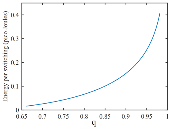
Figure 1: The relationship between energy consumed and probability of correctness $q$ of a single inverter built out of CMOS technology from [32]

.

In inexact computing, a function or algorithm $f$ which could be Boolean is computed in a noisy environment (see Figure 1) where the result can be erroneous. To formalize this notion, we postulate a reader as a function $\mathcal{R}:\{0,1\}^{n}\rightarrow\{0,1\}^{n}$ that “scrambles" the data by flipping (changing from $0$ to $1$ or vice-versa) some of the input bits. The result of the interference of the reader is that instead of evaluating the function using “correct” values, we end up evaluating $f\circ\mathcal{R}$.

The extent to which the reader obfuscates $\mathbf{x}$ depends on the energy invested. We are given an energy budget $\mathcal{E}\geq 0$ that can be apportioned into a vector of $n$ elements $\mathbf{e}=(e_{1},\cdots e_{n})$ while ensuring that $\sum_{i=1}^{n}e_{i}\leq\mathcal{E}$. Each of the $e_{i}$’s determines the probability with which our reader provides incorrect values of the corresponding $\mathbf{x}_{i}$. This effect is characterized by a transformation $\mathcal{F}:\mathbb{R}\rightarrow[0,1]$ such that for every $i$, the reader flips bit $i$ with probability $p_{i}=\mathcal{F}(e_{i})$, namely with probability $q_{i}=1-p_{i}$, $\mathbf{x}_{i}$ must be read correctly. In keeping with measured behavior of CMOS devices outlined above, $\mathcal{F}(e_{i})=1/2^{e_{i}}$. Clearly, the bigger $e_{i}$ is, the lower the chance that bit $i$ is flipped, and $\mathbf{p}=(p_{1},\cdots p_{n})$. Note that $\mathbf{p}$ is not a probability but rather, each $p_{i}$ is.

As mentioned in the previous section, this model is inspired by the behavior of physical gates such as the inverter as shown in Figure 1, or NAND gate as mentioned in [9], where an approximately exponential relationship between the error probability and the energy investment (such as energy investment in switching the value of the bit for Probability CMOS switch) was observed. The probability that an error occurs in a computational gate can be abstracted to be the probability of error of reading input bits to that gate. In reality, the error probability of a complex operation can be calculated by breaking down that operation to computational steps, and aggregate the error probability throughout the computational steps. However, analyzing at such level of details will quickly become infeasible. Our approach is to abstract away the details and place the error probability in certain key points in the computation. We believe this abstraction strikes the right balance between capturing what is essential on the one hand, while on the other hand retaining a level of simplicity in the model that allows researchers to be able to analyze algorithmic ideas.

3 Modeling inexactness in the context of Boolean functions

The previous section proposes the general model for inexactness in the general settings. In this section we want to examine the model further in the context of Boolean functions, a fundamental component of computer science theory and practice. In addition, for the next parts of the paper let us consider a more general version of Boolean functions $f:\{0,1\}^{n}\rightarrow\mathbb{N}$, because this version of Boolean functions are remarkably more popular in computing.

The overarching theme of this paper is inspired by the following: Given a function $f:\{0,1\}^{n}\rightarrow\mathbb{N}$, an energy budget $\mathcal{E}$, and a transformation function $\mathcal{F}$, what is the optimal way to distribute $\mathcal{E}$ to $n$ segments in order to minimize the obfuscation of the reader overall as $f$ is computed.

Consider an $n$-bit binary vector denoted $\mathbf{x}=(x_{1},x_{2},\ldots,x_{n})\in\{0,1\}^{n}$. For an index $i\in[n]$, where $[n]$ denotes $\{1,2,\ldots,n\}$, we use $\mathbf{x}^{\oplus i}$ to denote the vector that is identical to $\mathbf{x}$ apart from the bit $i$, which is “flipped” to $1-x_{i}$. Similarly, $\mathbf{x}^{(i\rightarrowtail 0)}$ and $\mathbf{x}^{(i\rightarrowtail 1)}$ denote the vectors identical to $\mathbf{x}$ with changing only $x_{i}$ to either $0$ or $1$ respectively, and $\mathbf{x}\sim\{0,1\}^{n}$ denotes a random value $\mathbf{x}$ uniformly drawn from $\{0,1\}^{n}$ and so $\mathbf{x}\sim\{0,1\}^{n}$. The key concept of influence of the $i$th bit for a function $f:\{0,1\}^{n}\rightarrow\mathbb{N}$ is

$$\mathsf{Inf}(i)\triangleq|(f(\mathbf{x})-f(\mathbf{x}^{\oplus i}))|,$$

where $\mathbf{x}$ is drawn uniformly from $\{0,1\}^{n}$. For convenience, we will refer to $\mathsf{Inf}(i)$ and the influence of index $i$ without explicitly referring to $\mathbf{x}$ when there is no ambiguity. We note that here, we differ from the traditional definition of influence [37] which is the expectation of $f:\{0,1\}^{n}\rightarrow\mathbb{N}$ with respect to $\mathbf{x}$ over all uniformly drawn vectors $\mathbf{x}$. However, it is technically more convenient in our case to explicitly express this expectation as $\mathbb{E}[\mathsf{Inf}(i)]$ averaged over all uniformly drawn vectors $\mathbf{x}$ and we will adopt this convention in the sequel. Furthermore, for convenience, we arrange the input bits so that $\mathbb{E}[\mathsf{Inf}(i)]\leq\mathbb{E}[\mathsf{Inf}(i+1)]$ for all $i<n$.

To understand the value of inexactness, influence and its expectation gives us the potential impact of assigning energy to a certain index $i$ preferentially over another index $j$ on the quality of the answer. Informally, we wish to assign more energy to variables associated with indices that have greater expected influence. To formalize this idea, let us define the total impact of a function $f$ given an energy vector $\mathbf{e}=(e_{i})_{i\leq n}$ and with induced error probabilities $\mathbf{p}=(p_{i})_{i\leq n}=(2^{-e_{i}})_{i\leq n}$ to be

$$\mathsf{TIm}_{f}(\mathbf{p})=\sum_{i\leq n}\mathbb{E}[\mathsf{Inf}(i)]\cdot p_{i}$$

We can then use total impact as the measure of how far from the correct values the function drifts given a particular energy vector $\mathbf{e}$. Now, given a function $f$ and an energy budget $\mathcal{E}$, our goal is to find $\mathbf{e}=(e_{i})_{i\leq n}$ that gives the best quality and thus minimize $\mathsf{TIm}_{f}$.

The most obvious and naive approach is to consider an energy vector that is influence oblivious where we allocate the energy equally to all the indices and therefore, $p_{i}=2^{-\mathcal{E}/n}$ for every $i$; this corresponds to the traditional architectural design that treats all bits equally. In this case, the expected total influence oblivious impact, is

$$\mathsf{TIm}_{f}(\mathbf{p}_{O})=2^{-\mathcal{E}/n}\sum_{i\leq n}\mathbb{E}[\mathsf{Inf}(i)]$$ (1)

In contrast, an influence aware allocation would be guided by the influence values to where indices with higher influence are assigned “proportionately” higher energy. Let $\mathsf{TIm}_{f}(\mathbf{p}_{A})$ be the expected total influence aware impact. Then, to understand the value of inexactness in the context of a function $f$, we define a figure of merit

$$\alpha=\frac{\mathsf{TIm}_{f}(\mathbf{p}_{O})}{\mathsf{TIm}_{f}(\mathbf{p}_{A})}$$ (2)

the ratio of the total impact of the oblivious assignment (numerator) to the aware assignment (denominator). Intuitively, the closer $\alpha$ is to 1, the less profitable it is to be influence aware as the naive influence oblivious solution can suffice almost as well. Conversely, $\alpha$ being large is a strong indication that influence aware solutions are likely to have a much higher impact on the quality of the solution.

To understand this point, let us consider a simple example of evaluating a binary string. Due to binary representation, the impact of an error grows as we progress from the least significant bit to the most significant bit. Thus, we should expect an influence oblivious approach to perform poorly when compared to one which is influence aware. To capture this notion of increased “weight” ubiquitous to computer science due to binary numbers we will compare influences as we step through the indices and define

$$\beta_{i}\triangleq\frac{\mathbb{E}[\mathsf{Inf}(i+1)]}{\mathbb{E}[\mathsf{Inf}(i)]}.$$ (3)

where $\beta_{i}$ is the relative influence of index $i+1$ compared to $i$. A straightforward observation is to note that functions with $\beta_{i}=1$ for all $1\leq i\leq n$ are functions where all the indices are equally influential; we will refer to such functions as being influence symmetric; classical problems such as parity and the OR function are examples. In contrast, influence asymmetric functions have $\beta_{i}>1$ for some indices $i$. We are particularly interested in functions where all $\beta_{i}$ values are equal and denoted $\beta$.

4 Existence of an Optimal Energy Assignment for any Boolean Function

To capture the possible benefits of inexactness aware approaches precisely, we formulate the following problem since the model is new and we wish to characterize its properties.

Problem 1.

[Basic Inexactness Problem] We define our basic inexactness problem comprising a basic inexact problem instance and an optimization criterion. The basic inexactness problem instance is a tuple $(f,\mathcal{E},\mathcal{F})$ where $f:\{0,1\}^{n}\to\mathbb{N}$ is a Boolean function, $\mathcal{E}$ is the inexactness energy amount, and $\mathcal{F}$ is the energy translation function. Given the inexactness problem instance $(f,\mathcal{E},\mathcal{F})$, our optimization criterion is to find an energy vector $(e_{1},\cdots,e_{n})$ whose elements sum to at most $\mathcal{E}$ (i.e., $\sum_{i}{e_{i}}\leq\mathcal{E}$) such that if $\mathbf{p}=(p_{1},\cdots,p_{n})$ where $p_{i}=\mathcal{F}(e_{i})$ for every $i$, then $\mathsf{TIm}_{f}(\mathbf{p})$ is minimized.

Without loss in generality, we assume that $\mathcal{F}(e)=1/2^{e}$. We will now show that an optimal solution always exists.

Theorem 1.

For every inexactness problem with any given any $\mathcal{E}$, a solution that minimizes the total impact exists and can be computed.

Proof.

Since $p_{i}=1/2^{e_{i}}$, we have that $e_{i}=-\log_{2}(p_{i})$. Therefore for the constraint $\sum_{i\leq n}e_{i}=\mathcal{E}$ we have:

$$\sum_{i\leq n}e_{i}=\mathcal{E}\iff\sum(\log(p_{i}))=-\mathcal{E}\iff\log(\prod p_{i})=-\mathcal{E}\iff\prod_{i\leq n}p_{i}=1/{2^{\mathcal{E}}}$$ (4)

Therefore we can redefine the inexact problem in Definition 1 as follows

Problem 2.

The problem denoted by $GP(f,\mathcal{E},\mathcal{F})$ is to find $\mathbf{e}=(e_{1},\cdots,e_{n})$ such that

• $\sum_{i\leq n}\mathbb{E}[\mathsf{Inf}(i)]p_{i}$ is minimized

• $p_{i}=1/2^{e_{i}}$

• $\prod_{i\leq n}p_{i}=1/{2^{\mathcal{E}}}$

• $0<p_{i}\leq 1$ for every $i\leq n$ ($p_{i}$ cannot be $0$)

To solve Problem 2 we use the AM-GM inequality according to which for every non-negative reals $a_{1},\cdots,a_{n}$ we have.

$$\frac{1}{n}\sum_{1\leq n}a_{i}\geq(\prod_{i\leq n}a_{i})^{\frac{1}{n}}$$ (5)

Since all the $p_{i}$ and the $\mathbb{E}[\mathsf{Inf}(i)]$ are non-negative, we can apply the AM-GM inequality to get:

$$\frac{1}{n}\sum_{i\leq n}\mathbb{E}[\mathsf{Inf}(i)]p_{i}\geq(\prod_{i\leq n}\mathbb{E}[\mathsf{Inf}(i)]p_{i})^{\frac{1}{n}}$$ (6)

Thus,

$$\sum_{i\leq n}\mathbb{E}[\mathsf{Inf}(i)]p_{i}\geq n(\prod_{i\leq n}\mathbb{E}[\mathsf{Inf}(i)]\prod_{i\leq n}p_{i})^{\frac{1}{n}}$$ (7)

Since we have a constraint that $\prod_{i\leq n}p_{i}=1/{2^{\mathcal{E}}}$, we all in all have that:

$$\sum_{i\leq n}\mathbb{E}[\mathsf{Inf}(i)]p_{i}\geq n(\prod_{i\leq n}\mathbb{E}[\mathsf{Inf}(i)]2^{-\mathcal{E}})^{\frac{1}{n}}$$ (8)

Recall that we need to find values for $p_{i}$ such that $\sum_{i\leq n}\mathbb{E}[\mathsf{Inf}(i)]p_{i}$ is minimized. Since no matter what values of $p_{i}$ we choose, the left side of the equation above will always be at least as the right side of the equation, minimization will come only when both sides are equal. In AM-GM we have that equality is reached when $\mathbb{E}[\mathsf{Inf}(i)]p_{i}$ is identical for all $i$. Using this we can now establish $p_{i}$ as follows. Assuming $\mathbb{E}[\mathsf{Inf}(i)]p_{i}=k$ for every $i$, we get

$$nk=n(\prod_{i\leq n}\mathbb{E}[\mathsf{Inf}(i)]2^{-\mathcal{E}})^{\frac{1}{n}}.$$ (9)

Thus,

$$k=(\prod_{i\leq n}\mathbb{E}[\mathsf{Inf}(i)]2^{-\mathcal{E}})^{\frac{1}{n}}.$$ (10)

Therefore for every $i\leq n$ we have

$$p_{i}=(\prod_{i\leq n}\mathbb{E}[\mathsf{Inf}(i)]2^{-\mathcal{E}})^{\frac{1}{n}}/\mathbb{E}[\mathsf{Inf}(i)]$$ (11)

and setting $e_{i}=-\log(p_{i})$ solves the problem as required. ∎

It is not always clear how such an influence aware energy assignment can be efficiently computed. Even the task of determining whether $\mathbb{E}[\mathsf{Inf}(i)]>0$ for a bit $i$ is a co-NP-hard problem as it encompasses asking whether the given CNF formula has no satisfying assignment.

5 Where does inexactness help?

We have seen that for a Boolean function, there always exists an optimal energy vector that minimizes the total impact. We now ask when exactly it pays to be influence aware? We shed some light into this question by examining the ratio $\alpha$ of the two extreme cases where for all $i$ $\beta_{i}=\beta$ a constant greater than 1, and the case where $\beta$ is 1. Recall that $\alpha$ is the ratio between the expected total influence oblivious impact and the expected total influence aware impact and $\beta_{i}$ is the ratio between the expected influence of bit $i+1$ and bit $i$.

For a given inexactness problem $(f,\mathcal{E},\mathcal{F})$, let $\mathbf{e}=(e_{1},e_{2},\ldots,e_{n})$ be the optimal energy vector (with corresponding error probability vector $\mathbf{p}=(p_{1},p_{2},\ldots,p_{n})$) obtained by the influence aware solution.

Influence Aware Investments

We now focus on the important case when all the $\beta_{i}$ values equal a common constant value $\beta$. This special case is in fact quite common and is exemplified by our previous example of evaluating a binary bit string where the influence of bit values decrease exponentially, in the context of binary numbers.

Theorem 2.

Let $f:\{0,1\}^{n}\to\mathbb{N}$ be a Boolean function with parameter $\beta>1$. Then, the corresponding $\alpha$ is at least $\Omega\left(\frac{\beta^{n/2}}{n}\right)$, thereby implying that an influence aware investment is exponentially better (with respect to $n$) than its influence oblivious counterpart.

Proof.

We first have that

$$GM=(\prod_{i<n}\mathbb{E}[\mathsf{Inf}(i)])^{1/n}=(\mathbb{E}[\mathsf{Inf}(1)]^{n}\prod_{i=0}^{n-1}\beta^{i})^{1/n}=\mathbb{E}[\mathsf{Inf}(1)]\beta^{(n-1)/2}$$

and

$$AM=1/n(\sum_{i\leq n}\mathbb{E}[\mathsf{Inf}(i)])=1/n(\mathbb{E}[\mathsf{Inf}(1)]\sum_{i=0}^{n-1}\beta^{i})=\frac{\mathbb{E}[\mathsf{Inf}(1)]}{n}\frac{\beta^{n}-1}{\beta-1}$$

Therefore we have that

$$\alpha=AM/GM=\frac{\beta^{n}-1}{n\beta^{(n-1)/2}(\beta-1)}$$

This ratio is $\Omega(\frac{\beta^{n/2}}{n})$ when $\beta>1$. ∎

To continue the example of evaluating $n$-bit binary strings, we present the following.

Corollary 1.

The value of $\alpha$ for Binary Evaluation (BE) function $f:\{0,1\}^{n}\to\mathbb{N}$ that takes a binary input and returns the decimal evaluation of that input is at least $\Omega\left(\frac{2^{n/2}}{n}\right)$.

Influence Oblivious Investments

To reiterate, formally, a Boolean function $f$ is influence-symmetric if all of the bits of $f$ have the same influence (i.e., $\mathsf{Inf}(i)=\mathsf{Inf}(j)$ for every $i\neq j$). Recall that from the definition of $\alpha$, we see that if $f$ is an influence-symmetric function then $\alpha=1$. An important class of Boolean functions are the symmetric Boolean functions defined as the set of functions $f$ such that for all $\mathbf{x}$ and any permutation $\sigma$, $f(\mathbf{x})=f(\sigma(\mathbf{x}))$ and therefore changing the order of the bits does not change the output of the function. We now have:

Theorem 3.

The influence oblivious assignment is an optimal energy distribution for influence-symmetric Boolean functions. Furthermore, every symmetric function is also influence-symmetric, so an influence oblivious investment is optimal.

Proof.

The key observation that we need to make first is that symmetric functions $f$ can be evaluated just by counting the number of 1’s in the input. Let $d_{j}\triangleq f(x^{j})$, where $x^{j}\in\{0,1\}^{n}$ has exactly $j$ 1’s. Let us consider $\mathsf{Inf}(1)$. What is the probability that $\mathsf{Inf}(1)$ takes the value, say, $a$? To answer this, let $J_{a}\subset[n]$ denote the set of all $j$ such that $|d_{j}-d_{j-1}|=a$. Then, clearly, $\mathsf{Inf}(1)=a$ with probability $\sum_{j\in J_{a}}\frac{\binom{n-1}{j-1}}{2^{n}}$. This same argument can be repeated for obtaining $\Pr[\mathsf{Inf}(i)=a]$. Thus, the random variables $\mathsf{Inf}(i)$ and $\mathsf{Inf}(i^{\prime})$, $i\neq i^{\prime}$, have the same distributions, thereby implying that $f$ is influence-symmetric. ∎

Let us consider the parity function $\mathsf{XOR}(\mathbf{x})$ – a quintessential symmetric function – that outputs 1 when the number of 1’s in $\mathbf{x}$ is odd, and $0$ otherwise. In this case, the $\mathsf{Inf}(i)=1$ for all $i$. Thus, the $\mathsf{TIm}(f,\mathcal{E})=n2^{\mathcal{E}/n}$, and this matches the total influence of the assignment that is influence oblivious wherein each bit is assigned energy $\mathcal{E}/n$. Thus, $\alpha=1$ for $\mathsf{XOR}$.

6 The influence ratio and PAC learning

Machine learning has been one of the most popular topics in computer science for decades. In this section, we would like to establish a direct relation between the influence ratio $\beta$ and a widely studied form of theoretical machine learning called Probably Approximate Correct (PAC) Learning where Boolean functions are learned with some margin for error. By exploring the relation between the concepts of fixed $\beta$ and PAC learning, we show that a function is more PAC-learnable if its influence ratio is greater than 1. Thus, this establishes the connection between the cases where machine learning performs well and the cases which can benefit from an influence aware approach.

In this section, we use an alternative more general form of Boolean functions $f:\{-1,+1\}^{n}\to\mathbb{R}$. This form is widely used in the study of PAC learning and analysis of Boolean functions. For a subset $S\subseteq[n]$ let $x^{S}=\prod_{i\in S}x_{i}$ where every $x_{i}\in\{-1,1\}$.

For a Boolean function $f$, another way to describe $f$ is as a mutli-polynomial called the Fourier expansion of $f$,

$$f(\mathbf{x})=\sum_{S\subseteq[n]}\hat{f}(S)x^{S}$$

where the real number $\hat{f}(S)$ is called the coefficient of $f$ on $S$. Then we have from [37] that the influence of a bit $i$ is as follows.

Definition 1.

Define $Var(i)=\frac{1}{4}E[\mathsf{Inf}(i)^{2}]$,

Claim 1.

For every $i\leq n$ $Var(i)=\sum_{S\subseteq[n],i\in S}\hat{f}(S)^{2}$.

The proof, as well as more on analysis of Boolean functions can be found in [37].

Definition 2.

Let $\epsilon>0,0\leq k\leq n$. A function $f:\{0,1\}^{n}\rightarrow\Re$ is called $\epsilon$-concentrated up to degree $k$, if $\sum_{S\subseteq[n],|S|>k}\hat{f(S)}^{2}<\epsilon$.

The notion of $\epsilon$-concentration up to degree $k$ is particularly interesting as it allows us to efficiently learn the function.

Theorem 4 (The "Low-Degree Algorithm" from page 81 in [37]).

Let $k\geq 1$ and let $C$ be a concept class for which every function $f:\{-1,1\}^{n}\rightarrow\{-1,1\}$ in $C$ is $\epsilon/2$-concentrated up to degree $k$. Then $C$ can be learned from random examples only with error $\epsilon$ in time poly$(n^{k},1/\epsilon)$.

We are ready to state our main theorem, which states that having influence ratio $\beta>1$ implies PAC learnability.

Note that quite often we do not get an exact measure $\beta$, for the influence ratio $1\leq\beta\leq\frac{\mathsf{Inf}(i+1)}{\mathsf{Inf}(i)}$ of a function, and it is much easier to obtain lower and upper bounds $\beta_{1},\beta_{2}$ such that $1\leq\beta_{1}\leq\beta\leq\beta_{2}$. By using these assumptions, and an additional bound $\mathsf{Inf}$ for which $\mathsf{Inf}(n)<\mathsf{Inf}$ we can say the following . Given $\epsilon>0$ calculate constant $k>0$ such that

$$\mathsf{Inf}\cdot\frac{\beta_{1}^{-k}}{\beta_{1}-1}<\epsilon/2$$ (12)

For simplicity denote $\mathsf{Inf}^{f}(n)$ the parameter $\mathsf{Inf}(n)$ for the specific function $f$. Then we have.

Theorem 5.

Let $C$ be a concept class and $\beta_{1},\beta_{2}\geq 1$, such that every function $f:\{-1,1\}^{n}\to\{-1,1\}$ in $C$ has $\beta_{f}$ where $\beta_{1}\leq\beta_{f}\leq\beta_{2}$, and such that $\mathsf{Inf}^{f}(n)\leq\mathsf{Inf}$ for some given parameter $\mathsf{Inf}>0$, and let $\epsilon>0$. Then $C$ can be learned from random examples with only error $\epsilon$ in time $poly(n^{k},1/\epsilon)$.

The proof of the theorem can be found in Appendix A.

7 Modeling inexactness in the context of sorting

We have been studying the idea of inexactness applied to Boolean functions. However, in real world applications, not all computational tasks are Boolean functions. Hence in this section, we examine the problem of sorting, an important computing task, to illustrate the benefit of influence aware investments.

Here we employ a setting wherein the data is an array $C$ of $N$ items stored in the “cloud” and a local computer called the client must compute a sorted ordering of the data. We begin with each data item $C[j]$, $1\leq j\leq N$, being $n$ bits drawn uniformly at random from $\{0,1\}^{n}$ representing integers in the range $[0,2^{n}-1]$. Since $C$ is in the cloud, the client can only access the data items indirectly through a predefined functions $\mathsf{Compare}(a,b,\mathbf{e})$, where $a$ and $b$ are two indices of the array $C$ and $\mathbf{e}$ is an energy vector. Since comparison seeks to find the most significant bit in which $C[a]$ and $C[b]$ differ, it employs bit-wise comparison. Thus, $\mathbf{e}$ serves the purpose of apportioning energy values across the bits. The client’s goal is to compute a permutation of $[N]\triangleq\{1,2,\ldots,N\}$ that matches the sorted ordering of $C$.

Our outcome will be an approximation of the correctly sorted ordering where, in the spirit of inexactness, minor errors that wrongly order numbers close in magnitude are more acceptable than egregious errors that reorder numbers that differ a lot. Thus, we measure sortedness using a measure that we call the weighted Kendall’s $\tau$ distance [21] that we now seek to define. We establish some notations first. Let $C^{*}$ denote the sorted permutation of the arbitrary array $C$. Consider two indices $a$ and $b$, both in the range $[1,N]$. Let $X(a,b)$ be an indicator random variable that is 1 when $C[a]$ and $C[b]$ are ordered differently in $C$ and $C^{*}$, and 0 when they are ordered the same way. The classical Kendall’s $\tau$ distance [28] counts the number of inversions and is defined as $\sum_{a\neq b}X(a,b)$. We are however interested in the weighted Kendall’s $\tau$ distance of $\pi$ denoted $\mathsf{wkt}^{C}()$ and it is defined as

$$\mathsf{wkt}^{C}\triangleq\sum_{a\neq b}\left[|C[a]-C[b]|\cdot X(a,b)\right]$$ (13)

The intuition behind this measure is that bigger difference between two numbers having incorrect relative order should result in bigger penalty, and vice versa. A reasonable inexact comparison scheme should have a smaller error chance for numbers that are farther apart - this is correct in the case of comparing using inexactness aware energy allocation scheme as we will see in this section.

Now, let us abuse the notation and use $\mathsf{wkt}^{C}(\mathbf{e})$ to denote the expected weighted Kendall’s $\tau$ distance of the permutation that we receive when we perform quicksort on input array $C$ using energy vector $\mathbf{e}$. Note that this value is averaged over all the runs of quicksort, with the random factors being the pivot choices of quicksort and the comparison error from inexactness:

$$\mathsf{wkt}^{C}(\mathbf{e})\triangleq\mathbb{E}_{C^{\mathbf{e}}}\left[\mathsf{wkt}^{C^{\mathbf{e}}}\right]$$ (14)

where $C^{\mathbf{e}}$ denotes a permutation of array $C$ after quicksort using energy vector $\mathbf{e}$.

In the next part of this section we are interested in analyzing the ratio of the expected weighted Kendall’s $\tau$ distance using inexactness oblivious energy to its inexactness aware energy counterpart (the expectation is taken over all possible input arrays $C$)

$$\alpha^{*}\triangleq\mathbb{E}_{C}[\mathsf{wkt}^{C}(\mathbf{e_{\sf o}})]/\mathbb{E}_{C}[\mathsf{wkt}^{C}(\mathbf{e_{\sf a}})]\,$$ (15)

which is analogous to the ratio $\alpha$ defined for Boolean functions. Our goal is to show that this ratio grows exponentially (in $n$). For the energy aware case the energy vector $\mathbf{e_{\sf a}}=(1,2,\ldots,n)$, thereby assigning higher energy values to higher order bits. On the other hand, for the energy oblivious case, we use equal energy for all the bits, so the energy vector is $\mathbf{e_{\sf o}}=(\frac{n+1}{2},\frac{n+1}{2},\cdots,\frac{n+1}{2})$. Both the inexactness aware and the inexactness oblivious algorithms employ quicksort using $\mathsf{Compare}(\cdot,\cdot,\cdot)$ functions, but with their respective energy vectors.

In the sequel theorems and proofs, we will use $I(a,b,\mathbf{e})$ to denote the event that the comparison between two numbers $a$ and $b$ is incorrect using the energy vector $\mathbf{e}$. We use $Q(a,b,\mathbf{e})$ to denote the event that the quicksort algorithm with input $C$ using energy vector $\mathbf{e}$ results in two numbers $a$ and $b$ having the incorrect relative positions (for simplicity we omit the input array $C$ from this notation). For simplicity, we will assume that the elements in our input array are distinct. Finally, from its definition in equations 13 and 14 and from linearity of expectation, $\mathsf{wkt}^{C}(\mathbf{e})$ can be calculated as follows

$$\mathsf{wkt}^{C}(\mathbf{e})=\sum_{1\leq a<b\leq n}|C[a]-C[b]|\cdot\Pr[Q(C[a],C[b],\mathbf{e})]$$ (16)

We state our desired result of the lower bound of $\alpha*$ as follows. The proof of this theorem can be found in Appendix B.

Theorem 6.

The ratio $\alpha^{*}$ is $\Omega(\frac{2^{n/2}}{N\log N})$.

The advantage of influence-aware approach can be shown not only through the ratio $\alpha*$ which is based on the difference between the two approaches’ average weighted Kendall’s $\tau$ distance over all inputs, but also through the distance difference of the majority of individual inputs. Let us define a good input as one for which the inexactness aware assignments results in an exponentially lower value of weighted Kendall’s $\tau$ distance; the rest of the inputs are called bad. More specifically, a good input $C$ is such that the ratio between $\mathsf{wkt}^{C}(\mathbf{e_{\sf o}})$ and $\mathsf{wkt}^{C}(\mathbf{e_{\sf a}})$, the expected weighted Kendall’s $\tau$ of quicksort with input $C$ under energy oblivious and energy awareness, is $\Omega(\frac{2^{n/6}}{N\log N})$. Let $g$ and $b$ denote the number of good and bad inputs, respectively. We will show that $g/b$ is exponential in $n$.

Theorem 7.

The ratio of the number of good vs. bad inputs is $\Omega(\frac{2^{n/3}}{N^{2}})$. Therefore, as $n\to\infty$, $g/b\to\infty$.

The proof of this theorem can be found in Appendix C

8 Variable Precision Computation

In practice, manufacturers usually lack the resource to assign a different level of energy to every bit in a chip. A more practical approach is that only $\gamma$ different levels of energy are assigned to the bits, usually with the lowest energy level being 0. This approach is usually referred to as variable precision computation, and has been studied in some works such as  [24], owing to its simplicity and effectiveness.

In this section, we will focus in the scenario where $\gamma=2$, i.e. a large proportion of the energy is equally focused on the most significant $\frac{n}{k}$ bits, where a small proportion, if not none, of the energy is assigned to the remaining $n(1-1/k)$ bits. We denote this energy vector $\mathbf{e_{\sf t}}$. Since the total energy is $\approx n^{2}/2$, $\mathbf{e_{\sf t}}=\{0,0,\ldots 0,2nk,\ldots 2nk\}$.

The goal of this section is to study the effect of using this energy vector compared to the inexactness oblivious approach for basic functionalities, which we again use sorting and the weighted Kendall’s $\tau$ metric as an example. We are interested in bounding the value of the ratio between ${\mathbb{E}_{C}[\mathsf{wkt}^{C}(\mathbf{e_{\sf o}})]}$ $/{\mathbb{E}_{C}[\mathsf{wkt}^{C}(\mathbf{e_{\sf t}})]}$ which is analogous to $\alpha^{*}$ in Section 7, and the ratio between good and bad inputs, whereas bad (and good) inputs are generally the ones that make $\mathsf{wkt}^{C}(\mathbf{e_{\sf o}})$ $/{\mathsf{wkt}^{C}(\mathbf{e_{\sf t}})}$ exponential in $n$ following the convention in Section 7.

Toward that goal, we prove the following two theorems. The combined result of the two theorems gives us an estimate of a ’good’ truncation ratio $k$, which is inside the interval $(\frac{5}{3},4)$.

Theorem 8.

Let $k$ be a parameter and assume we use an energy allocation scheme $\mathbf{e_{\sf t}}$ where energy is divided equally on $\frac{n}{k}$ most significant bits. Then, for an arbitrary input array $C$ drawn from the uniform random distribution,

$$\Pr\left[\frac{\mathsf{wkt}^{C}(\mathbf{e_{\sf o}})}{\mathsf{wkt}^{C}(\mathbf{e_{\sf t}})}=O(\frac{2^{n(k-5/3)/6}}{N\log N})\right]=O(\frac{N^{2}}{2^{\frac{n}{max(3,k)}}})$$

Consequently, for constant $k>5/3$, if we define bad inputs to be the ones that make the ratio $\frac{\mathsf{wkt}^{C}(\mathbf{e_{\sf o}})}{\mathsf{wkt}^{C}(\mathbf{e_{\sf t}})}$ $O(\frac{2^{n(k-5/3)/6}}{N\log N})$ and good inputs to be the remaining, then the ratio between good and bad inputs is at least $\Omega(\frac{2^{n/max(3,k)}}{N^{2}})$.

Theorem 9.

Let $k$ be a parameter and assume we divide energy on $\frac{n}{k}$ most significant bits. Then, for $k<4$, the ratio $\frac{\mathbb{E}_{C}[\mathsf{wkt}^{C}(\mathbf{e_{\sf o}})]}{\mathbb{E}_{C}[\mathsf{wkt}^{C}(\mathbf{e_{\sf t}})]}$ is exponential in $n$.

Remarks The variable precision energy allocation scheme is a more practical approach to inexactness where the energy is focused only on the most significant $n/k$ bits. In this section, we have shown that for a value of $k$ in the interval $(\frac{5}{3},4)$, sorting using variable precision energy allocation scheme is exponentially better than using inexactness oblivious energy allocation in the weighted Kendall’s $\tau$ metric. This is true for both the average case (Theorem 9) and for most of the possible inputs with only an exponentially small number of exceptions (Theorem 8). Note that the specific value $\frac{5}{3}<k<4$ resulted from the analysis with $\approx\frac{n^{2}}{2}$ total energy. For the analyses using different levels of total energy and different restrictions (such as the number $\gamma$ of distinct energy levels), we might arrive at different schemes of energy distribution. Nevertheless, the core principle of inexactness should remain applicable.

9 Concluding remarks

The algorithmic end of computing has a rich history of examples such as randomization [45, 46] and approximation algorithms [49], and combined approaches such as fully polynomial Randomized approximation schemes (FPRAS) [25] which departed radically from traditional computing philosophy of guaranteeing correctness. Specifically, they embraced the possibility that computations can yield results that are not entirely correct while offering (potentially) significant savings in resources consumed, typically running time. Despite this relaxed expectation on the the quality of their solutions, randomized and approximation algorithms were always deployed on reliable computing systems. In contrast, inexact computing crucially differs by advocating the use of “unreliable” computing architectures and systems directly and thus, blend in the behavior from the platform on which it is executing directly into the algorithm. Thus, one can view the inexactness in our model as a way of extending the principles of randomization and approximation down to the hardware level, thereby improving the overall gains that we can garner. Thus, the ability to lower cost by lowering energy, and its allocation to different parts of the computation guided by influence are made explicit and can be managed by the algorithm designer. By demonstrating the value of this idea in canonical and illustrative settings, namely theory of Boolean functions, PAC learning, inexact sorting, we aimed to have demonstrated its value in a range of settings. In principle, the model we have introduced and whose value we demonstrated through several foundational building blocks is truly general in the following sense: given any computing engine and hence an instance of our model, an algorithm can be designed and evaluated. Additionally, due to its theoretical generality, our model parameters allow us to assert the cost and quality of algorithms as functions of parameter values and thus can, in the spirit of the foundations of computer science, be characterized as theorems are true asymptotically.

In addition to extending the notion of randomized and approximate computation to the hardware level, we believe that the framework of inexactness that we have introduced can seamlessly extend beyond its immediate motivation from CMOS technology. At its core, the potential for inexactness stems from the notion of influence that is orthogonal to the computing technology that is employed. In our work, we have framed the model using CMOS principles and the concomitant error function that decays exponentially with energy. Alternative technologies like quantum computing may offer slightly different modeling parameters, but we believe that the core principles based on the notion of influence will remain intact and effective. Thus, we hope that our work will enable future work resulting in a principled injection of inexactness in a wide range of contexts.

Appendix A Proof of theorem 5 in section 6

We show that given $(\epsilon,f)$, by obtaining the fixed $\beta$ from the function $f$ we can provide $k$ such that $f$ is concentrated with respect to $(\epsilon,k)$. The close relation between a concentrated and learnable functions will lead us to a result about the capability of the function of being learnable.

Lemma 1.

Let $f$ be a function $f:\{0,1\}^{n}\rightarrow\Re$ such that $\sum_{i>k}Var(n-i)<\epsilon$ for $\epsilon>0$ and $k\leq n$. Then $f$ is $\epsilon$-concentrated up to degree $k$.

Proof.

From Claim 1, for every $i<n$ we have

$$Var(n-i)=\sum_{S\subseteq[n],n-i\in S}\hat{f(S)}^{2}$$ (17)

Now let $S$ be a subset of size bigger than $k$. Then there must be an element $i>k$ such that $n-i\in S$. Therefore $\{S|S\subseteq[n],|S|>k\}\subseteq\{S|S\subseteq[n],\exists(i>k)n-i\in S\}$. Therefore we have that

$$\sum_{S\subseteq[n],|S|>k}\hat{f(S)}^{2}\leq\sum_{S\subseteq[n],\exists(i>k)n-i\in S}\hat{f(S)}^{2}=\sum_{i>k}\sum_{S\subseteq[n],n-i\in S}\hat{f(S)}^{2}=\sum_{i>k}Var(n-i)<\epsilon$$ (18)

Therefore $f$ is $\epsilon$-concentrated up to degree $k$. ∎

Given that the influences $\mathsf{Inf}(i)$ are all positive random variables we have an easy lemma.

Lemma 2.

Let $f$ be a function $f:\{0,1\}^{n}\rightarrow\Re$ such that $\sum_{i>k}\mathsf{Inf}(n-i)<\epsilon$ for $1>\epsilon>0$ and $k\leq n$. Then $f$ is $\epsilon$-concentrated up to degree $k$.

Proof.

$\sum_{i>k}\mathsf{Inf}(n-i)<\epsilon<1$ implies $\sum_{i>k}Var(n-i)<\epsilon$ because of $0\leq\mathsf{Inf}(i)<1$ from the definition of influence. ∎

With Lemma 2, we are ready to prove our main theorem of this section.

Proof of Theorem 5.

For every function $f$ in $C$ we have that $\beta_{1}\leq\beta_{f}$. Then we have:

$$\sum_{i>k}\mathsf{Inf}(n-i)=\mathsf{Inf}(n)\frac{\beta_{f}^{-k}-\beta_{f}^{-n+1}}{\beta_{f}-1}<\mathsf{Inf}\frac{\beta_{1}^{-k}}{\beta_{1}-1}<\epsilon/2$$ (19)

Therefore we have from Lemma 2 that every function $f$ in $C$ is $\epsilon/2$-concentrated up to degree $k$. By the “Low-Degree” Algorithm, the learnability from random examples with error $\epsilon$ in time $poly(n^{k},1/\epsilon)$ follows immediately.

∎

It is interesting to note that the opposite of Lemma 2 is not always correct. Specifically, it is easy to construct a function $f$ for which $\hat{f(\{i\})}=1$ for every bit $i$, and $\hat{f(S)}=0$ (or is very small) for every set $S$ of size at least $2$. Such a function is $\epsilon$-concentrated up to degree $2$ but no matter what the order of bits are for every $i$, $\mathsf{Inf}(i)\geq\hat{f(\{i\})}=1$ So for every $k<n$ $\sum_{n-i>k}\mathsf{Inf}(n-i)\geq 1$. Studying of when exactly a small concentration lead to small influence ratio is a matter of future work.

Appendix B Proof of Theorem 6 in section 7

First we prove some lemmas which will be useful for the rest of this section.

Lemma 3.

Consider two arbitrary $n$-bit integers $a<b$. Then

$$\Pr[I(a,b,\mathbf{e_{\sf a}})]<\frac{8}{b-a}$$

Proof.

Consider $n\geq i\geq 1$ the first bit where $a$ and $b$ differ ($i=n$ means $a$ and $b$ differ from the most significant bit).

The probability that comparison is wrong before getting to bit $i$ is less than or equal to the sum of the probabilities that the comparison is wrong at bit $j>i$, which is $=1/2^{n}+1/2^{n-1}+\ldots+1/2^{i+1}=1/2^{i}-1/2^{n}$.

The probability that the comparison is wrong at bit $i$ is $1/2^{2i}$ since the bits $i$ in $a$ and $b$ must both be flipped for this to happen. The probability that the comparison is wrong after bit $i$ is $<1/2^{i-1}$ as exactly one bit $i$ in either $a$ and $b$ must be flipped and the remaining of $C[a]$ has a probability $1/2$ to be compared bigger than the remaining of $b$.

Summing all these, we have $\Pr[I(a,b)]<1/2^{i-2}$.

Note that when $i$ is the first bit that $a$ and $b$ differ, we have $2^{i+1}>b-a\geq 1$. Therefore, $(b-a)\Pr[I(a,b)]<\frac{1}{2^{i-2}}\cdot 2^{i+1}=8$ and the result follows.

∎

Lemma 4.

Consider an arbitrary array $C$ of $N$ $n$-bit integers. Then

$$\mathsf{wkt}^{C}(\mathbf{e_{\sf a}})=O(N^{2}\log N)$$

Proof.

We will prove the inequality using result from Lemma 3. Consider a random pivot $C[j]$. Note that once the pivot $C[j]$ splits $C[a]$ and $C[b]$ to two sides, then the relative position of $C[a]$ and $C[b]$ is determined. In particular if $C[j]$ splits $C[a]$ to the bigger side and $C[b]$ to the smaller side then the event that split is incorrect at pivot $C[j]$, which we denote $Q(C[a],C[b],C[j],\mathbf{e_{\sf a}})$, happens. There are 4 cases:

• Case 1: $C[a]<C[b]<C[j]$. In this case $Q(C[a],C[b],C[j],\mathbf{e_{\sf a}})$ happens if only $I(C[a],C[j])$ happens. Therefore in this case

  $$\begin{split}\Pr[Q(C[a],C[b],C[j],\mathbf{e_{\sf a}})]&=\Pr[I(C[a],C[j],\mathbf{e_{\sf a}})]\cdot(1-\Pr[I(C[b],C[j],\mathbf{e_{\sf a}})])\\ &<\Pr[I(C[a],C[j],\mathbf{e_{\sf a}})]<\frac{8}{C[j]-C[a]}<\frac{8}{|C[a]-C[b]|}\end{split}$$

• Case 2: $C[j]<C[a]<C[b]$. In this case $Q(C[a],C[b],C[j],\mathbf{e_{\sf a}})$ happens if only $I(C[b],C[j],\mathbf{e_{\sf a}})$ happens. Therefore again

  $$\begin{split}\Pr[Q(C[a],C[b],C[j],\mathbf{e_{\sf a}})]&=\Pr[I(C[b],C[j],\mathbf{e_{\sf a}})].(1-\Pr[I(C[a],C[j],\mathbf{e_{\sf a}})])\\ &<\Pr[I(C[b],C[j],\mathbf{e_{\sf a}})]<\frac{8}{C[j]-C[b]}<\frac{8}{|C[a]-C[b]|}\end{split}$$

• Case 3: $C[a]<C[j]<C[b]$. In this case $Q(C[a],C[b],C[j],\mathbf{e_{\sf a}})$ happens if both $I(C[b],C[j],\mathbf{e_{\sf a}})$ and $I(C[a],C[j],\mathbf{e_{\sf a}})$ happen. Therefore, noting that $\Pr[I(x,y,\mathbf{e_{\sf a}})]<1/2$ for all $x\neq y$

  $$\begin{split}\Pr[Q(C[a],C[b],C[j],\mathbf{e_{\sf a}})]&=\Pr[I(C[b],C[j],\mathbf{e_{\sf a}})]\cdot\Pr[I(C[a],C[j],\mathbf{e_{\sf a}})]\\ &<\frac{8}{C[j]-C[a]}\cdot\frac{8}{C[b]-C[j]}<\frac{64}{C[a]-C[b]}\end{split}$$

• Case 4: either $a=j$ or $b=j$. In this case, $\Pr[Q(C[a],C[b],C[j],\mathbf{e_{\sf a}})]=\Pr[I(C[a],C[b],\mathbf{e_{\sf a}})]$.

Therefore, for all choices of pivot $C[j]$, $\Pr[Q(C[a],C[b],C[j],\mathbf{e_{\sf a}}]<\frac{64}{|C[a]-C[b]|}$. The probability of $Q(C[a],C[b],\mathbf{e_{\sf a}})$ happens is less than or equal to the sum of the probabilities that $Q(C[a],C[b],C[j],\mathbf{e_{\sf a}})$ happens for $C[j]$ all the pivots that $C[a]$ and $C[b]$ get compared to

$$\Pr[Q(C[a],C[b],\mathbf{e_{\sf a}})]\leq\sum_{j}\Pr[Q(C[a],C[b],C[j],\mathbf{e_{\sf a}})]$$

$$\leq 1.4\log N\Pr[I(C[a],C[b],\mathbf{e_{\sf a}})]<1.4\log N\frac{64}{|C[a]-C[b]|}$$

using the well-known result that the expected recursion depth of quicksort is $<1.4\log N$ (here we assume that the worst case of the version of quicksort that we use is not input-dependent). Therefore,

$$\Pr[Q(C[a],C[b],\mathbf{e_{\sf a}})]\cdot|C[a]-C[b]|<90\log N$$ (20)

for arbitrary $a,b$.

We can now evaluate $\mathsf{wkt}^{C}(\mathbf{e_{\sf a}})$ as follows.

$$\begin{split}\mathsf{wkt}^{C}(\mathbf{e_{\sf a}})&=\sum_{1\leq a<b\leq N}\left[|C[a]-C[b]|\cdot\Pr[Q(C[a],C[b],\mathbf{e_{\sf a}})]\right]\\ &\leq\sum_{1\leq a<b\leq N}90\log N\\ &<50N^{2}\log N.\end{split}$$ (21)

∎

Now we can use the lemmas developed to prove our main result of this section.

Proof of Theorem 6.

From Lemma 4 we know that for every input array $C$, $\mathsf{wkt}^{C}(\mathbf{e_{\sf a}})<50N^{2}\log N$. Thus,

$$\mathbb{E}_{C}[\mathsf{wkt}^{C}(\mathbf{e_{\sf a}})]<50N^{2}\log N$$ (22)

We now turn out attention to bounding $\mathbb{E}[\mathsf{wkt}^{C}(\mathbf{e_{\sf o}})]$ from below. Consider any input array $C$, two arbitrary indices $a,b$ and the first pivot of quicksort $C[j]$. The probability that $j=a$ or $j=b$ is $2/N$, and when this happens $\Pr[Q(C[a],C[b],C[j],\mathbf{e_{\sf o}})=\Pr[I(C[a],C[b],\mathbf{e_{\sf o}})]$. Thus

$$\Pr[Q(C[a],C[b],\mathbf{e_{\sf o}})]>\Pr[Q(C[a],C[b],C[j],\mathbf{e_{\sf o}})>\frac{2}{N}\cdot\Pr[I(C[a],C[b],\mathbf{e_{\sf o}})]$$ (23)

Now, because we are reasoning about expectation over all inputs $C$, we have:

$$\begin{split}\mathbb{E}_{C}[\mathsf{wkt}^{C}(\mathbf{e_{\sf o}})]&=\frac{N(N+1)}{2}\cdot\mathbb{E}_{0\leq c,d\leq 2^{n}-1}[|c-d|\cdot\Pr[Q(c,d,\mathbf{e_{\sf o}})]]\\ &>\frac{N(N+1)}{2}\cdot\frac{2}{N}\mathbb{E}_{0\leq c,d\leq 2^{n}-1}[|c-d|\cdot\Pr[I(c,d,\mathbf{e_{\sf o}})]]\end{split}$$ (24)

Let us now bound $\mathbb{E}_{0\leq c,d\leq 2^{n}-1}[|c-d|\cdot\Pr[I(c,d,\mathbf{e_{\sf o}})]]$. As before, consider $1\leq i\leq n$ as the index of the leading different bit of $c$ and $d$, denote $FD(c,d)=i$. We will reason about $\Pr[I(c,d,\mathbf{e_{\sf o}})]$. When $i<n$ the probability that the comparison is wrong is $>1/2^{n/2+2}$ since the comparison can be wrong at the very first bit. Thus,

$$\begin{split}&\mathbb{E}_{0\leq c,d\leq 2^{n}-1}[|c-d|\cdot\Pr[I(c,d,\mathbf{e_{\sf o}})]]\\ &=\mathbb{E}_{FD(c,d)=n}|c-d|\cdot\Pr[I(c,d,\mathbf{e_{\sf o}})|FD(c,d)=n]\cdot\Pr[FD(c,d)=n]\\ &+\mathbb{E}_{FD(c,d)<n}|c-d|\cdot\Pr[I(c,d,\mathbf{e_{\sf o}})|FD(c,d)<n]\Pr[FD(c,d)<n]\\ &>\mathbb{E}_{FD(c,d)=n}|c-d|\cdot\Pr[I(c,d,\mathbf{e_{\sf o}})|FD(c,d)=n]\cdot\Pr[FD(c,d)=n]\\ &=\frac{2^{n-1}}{3}.\frac{1}{2^{n/2+2}}\cdot\frac{1}{2}=\frac{2^{n/2-4}}{3}\end{split}$$ (25)

Therefore, from equation 21 and equation 25

$$\mathbb{E}_{C}[\mathsf{wkt}^{C}(\mathbf{e_{\sf o}})]>\frac{N+1}{48}2^{n/2}$$ (26)

The theorem follows from equation 22 and equation 26.

∎

Appendix C Proof of Theorem 7 in section 7

First let us prove a lemma

Lemma 5.

Consider an input array $C$ of $N$ integers drawn from the uniform random distribution over the set of all inputs. Then,

$$\Pr\left[\frac{\mathsf{wkt}^{C}(\mathbf{e_{\sf o}})}{\mathsf{wkt}^{C}(\mathbf{e_{\sf a}})}=\Omega(\frac{2^{n/6}}{N\log N})\right]=1-O(\frac{N^{2}}{2^{n/3}})$$

Proof.

From Lemma 4 we know that $\mathsf{wkt}^{C}(\mathbf{e_{\sf a}})<50N^{2}\log N$ for every input $C$. Thus we only need to calculate a concentration bound of $\mathsf{wkt}^{C}(\mathbf{e_{\sf o}})$ to arrive at our goal.

From equation 23 in the proof of Theorem 6, we know that for every pair of indices $a$ and $b$, $\Pr[Q(C[a],C[b],\mathbf{e_{\sf o}})]>\frac{2}{N}$ $\cdot\Pr[I(C[a],C[b],\mathbf{e_{\sf o}})]$, and thus

$$\begin{split}\mathsf{wkt}^{C}(\mathbf{e_{\sf o}})&=\sum_{a<b\leq N}|C[a]-C[b]|\cdot\Pr[Q(C[a],C[b],\mathbf{e_{\sf o}})]\\ &>\frac{2}{N}\sum_{a<b\leq N}|C[a]-C[b]|\cdot\Pr[I(C[a],C[b],\mathbf{e_{\sf o}})]\end{split}$$ (27)

Let us consider the case when $C[a]$ and $C[b]$ have the first different bit index $<n$, i.e. $FD(C[a],C[b])<n$. As stated before in the proof of Theorem 6, when $FD(C[a],C[b])<n$ we have $\Pr[I(C[a],C[b],\mathbf{e_{\sf o}})]>1/2^{n/2+2}$. For $\frac{N(N+1)}{2}$ pairs $C[a],C[b]$ there are at least $N(N+2)/2$ pairs having the same leading bit (this is a straight application of AM-GM inequality). On the other hand, if $C[a]$ and $C[b]$ are random numbers from the uniform distribution with the same leading bit, $|C[a]-C[b]|$ can be seen as the absolute difference of 2 uniformly random $(n-1)$-bit numbers. Now, for two $(n-1)$-bit numbers $c<d$ uniformly random, the probability distribution of $(d-c)$ is a triangle that connects points $(0,0)$, $(0,2^{n})$ and $(2^{n},0)$ in the coordinate system. From this probability distribution, we solve the probability that $d-c\leq 2^{2n/3}$ or $b-a\geq 2^{n}-2^{2n/3}$ is $\frac{1}{2^{n/3}}$.

Thus from equation 27 and the union bound, with probability $>1-\frac{N^{2}}{2^{n/3}}$ we have

$$\begin{split}\mathsf{wkt}^{C}(\mathbf{e_{\sf o}})&>\frac{2}{N}\sum_{a<b\leq N}|C[a]-C[b]|\cdot\Pr[I(C[a],C[b],\mathbf{e_{\sf o}})]\\ &>\frac{2}{N}\cdot\frac{N^{2}}{2}\cdot\frac{1}{2^{n/2+2}}\cdot 2^{2n/3}\\ &=\frac{N}{8}\cdot 2^{n/6}\end{split}$$ (28)

Thus, from Lemma 4

$$\Pr\left[\frac{\mathsf{wkt}^{C}(\mathbf{e_{\sf o}})}{\mathsf{wkt}^{C}(\mathbf{e_{\sf a}})}>\frac{N\cdot 2^{n/6}}{400N^{2}\log N}\right]>1-\frac{N^{2}}{2^{n/3}}$$ (29)

and the result follows. ∎

Our desired result follows immediately after the above lemma.

Proof of theorem 7.

From Lemma 6 the probability of an input $C$ drawn from the uniform random distribution over the set of all inputs being bad is $O(\frac{N^{2}}{2^{n/3}})$ and the theorem follows. ∎

Appendix D Proof of Theorem 8 and Theorem 9 in section 8

Similar to the previous section, we will first prove some useful lemmas.

Lemma 6.

Given two random number $a$ and $b$, if the first different bit index $FD(a,b)=i\geq n-n/k$ then

• $\Pr[I(a,b,\mathbf{e_{\sf t}})]<\frac{n-i+2}{2^{nk/2}}$

• $|a-b|\cdot\Pr[I(a,b,\mathbf{e_{\sf t}})]<\frac{2}{2^{n(k-2)/2}}$

Proof.

When $n/k$ bits has energy allocated, each bit gets $nk/2$ energy and therefore the probability that the reader reads that bit wrongly is $\frac{1}{2^{nk/2}}$. Consider an arbitrary input array $C$. Let us first examine $\Pr[I(a,b)]$ for $b>a$ arbitrary elements in $C$. Consider the index of the leading different bit of $a$ and $b$ $i$, i.e. $FD(a,b)=i$. For each index $j>i$, the probability that the comparison is incorrect at bit $i$ is $<1/2^{nk/2}$. If $i\geq n-n/k$, the probability that the comparison is incorrect before getting to bit $i$ is $<\frac{n-i}{2^{nk/2}}$. The probability that the comparison is incorrect at bit $i$ is $<\frac{1}{2^{nk}}$, and the probability that the comparison is incorrect after bit $i$ is $<1/2^{nk/2}$. Overall, we have the probability that the comparison is incorrect is $<\frac{n-i+2}{2^{nk/2}}$ if $FD(a,b)=i\geq n-n/k$.

The second statement follows from the first one. We note that if the leading different bit of $a,b$ is $i$ then $|a-b|<2^{i}$. Thus we have $|a-b|.\Pr[I(a,b,\pi_{t})]<2^{i}\cdot\frac{n-i+2}{2^{nk/2}}$. This expression is biggest when $i=n$, thus $|a-b|.\Pr[I(a,b,\pi_{t})]<\frac{2}{2^{n(k-2)/2}}$ if the index of the leading different bit of $a,b$ is $\geq n-n/k$. ∎

Lemma 7.

Given a random input array $C$ of $N$ $n$-bit numbers and two random index $a,b<N$. Then if $FD(C[a],C[b])=i\geq n-n/k$ then $\Pr[Q(C[a],C[b],\mathbf{e_{\sf t}})]\cdot|C[a]-C[b]|<\frac{2.8\log N}{2^{n(k-2)/2}}$.

Proof.

We will use results from Lemma 6. Let us again look at the 4 cases of pivot comparison. This time, we note that if $a<b<j$, $FD(a,j)\geq FD(a,b)$ (this is straightforward to check) and if $a<j<b$, either $FD(a,j)$ or $FD(b,j)=FD(a,b)$. We also note that if $FD(a,b)<n-n/k$, the comparison will be always be false since the bits after index $n-n/k$ always get flipped.

• Case 1: $C[a]<C[b]<C[j]$. In this case $Q(C[a],C[b],C[j],\mathbf{e_{\sf a}})$ happens if only $I(C[a],C[j])$ happens. Therefore in this case

  $$\begin{split}\Pr[Q(C[a],C[b],C[j],\mathbf{e_{\sf t}})]&=\Pr[I(C[a],C[j],\mathbf{e_{\sf t}})]\cdot(1-\Pr[I(C[b],C[j],\mathbf{e_{\sf t}})])\\ &<\Pr[I(C[a],C[j],\mathbf{e_{\sf t}})]\end{split}$$

  If $FD(a,b)\geq n-n/k$ then $FD(a,j)\geq n-n/k$, thus $\Pr[I(C[a],C[j],\mathbf{e_{\sf t}})]<\frac{2}{2^{n(k-2)/2}}\cdot\frac{1}{C[j]-C[a]}<\frac{2}{2^{n(k-2)/2}}\cdot\frac{1}{C[b]-C[a]}$, thus $\Pr[Q(C[a],C[b],C[j],\mathbf{e_{\sf t}})]\cdot|C[a]-C[b]|<\frac{2}{2^{n(k-2)/2}}$.

• Case 2: $C[j]<C[a]<C[b]$. In this case $Q(C[a],C[b],C[j],\mathbf{e_{\sf a}})$ happens if only $I(C[b],C[j],\mathbf{e_{\sf t}})$ happens. Therefore again

  $$\begin{split}\Pr[Q(C[a],C[b],C[j],\mathbf{e_{\sf t}})]&=\Pr[I(C[b],C[j],\mathbf{e_{\sf t}})].(1-\Pr[I(C[a],C[j],\mathbf{e_{\sf t}})])\\ &<\Pr[I(C[b],C[j],\mathbf{e_{\sf t}})]\end{split}$$

  Similar to the above case, in this case $\Pr[Q(C[a],C[b],C[j],\mathbf{e_{\sf t}})]\cdot|C[a]-C[b]|<\frac{2}{2^{n(k-2)/2}}$.

• Case 3: $C[a]<C[j]<C[b]$. In this case $Q(C[a],C[b],C[j],\mathbf{e_{\sf a}})$ happens if both $I(C[b],C[j],\mathbf{e_{\sf a}})$ and $I(C[a],C[j],\mathbf{e_{\sf a}})$ happen. Therefore,

  $$\begin{split}\Pr[Q(C[a],C[b],C[j],\mathbf{e_{\sf a}})]&=\Pr[I(C[b],C[j],\mathbf{e_{\sf a}})].\Pr[I(C[a],C[j],\mathbf{e_{\sf a}})]\end{split}$$

  Now, note that if $C[a]<C[j]<C[b]$, either $FD(C[a],C[j])$ or $FD(C[b],C[j])=FD(C[a],C[b])$. Assume it is $FD(C[a],C[j])$, then if $FD(C[a],C[b])\geq n-n/k$ then so is $FD(C[a],C[j])$. Thus we have $\Pr[Q(C[a],C[b],C[j],\mathbf{e_{\sf a}})]\leq\Pr[I(C[a],C[j],\mathbf{e_{\sf a}})]<\frac{n-i+2}{n^{nk/2}}$, and so $\Pr[Q(C[a],C[b],$ $C[j],\mathbf{e_{\sf a}})]\cdot|C[a]-C[b]|<2^{i}\cdot\frac{n-i+2}{n^{nk/2}}\leq\frac{2}{2^{n(k-2)/2}}$ as proved in lemma 6.

• Case 4: either $a=j$ or $b=j$. In this case, $\Pr[Q(C[a],C[b],C[j],\mathbf{e_{\sf a}})]=\Pr[I(C[a],C[b],\mathbf{e_{\sf a}})]$ and so $\Pr[Q(C[a],C[b],C[j],\mathbf{e_{\sf a}})]\cdot|C[a]-C[b]|<\frac{2}{2^{n(k-2)/2}}$.

Therefore, if $FD(C[a],C[b])=i\geq n-n/k$ then $\Pr[Q(C[a],C[b],C[j],\mathbf{e_{\sf a}})]\cdot|C[a]-C[b]|<\frac{2}{2^{n(k-2)/2}}$. Thus,

$$\begin{split}\Pr[Q(C[a],C[b],\mathbf{e_{\sf t}})]\cdot|C[a]-C[b]|&\leq\sum_{j}\Pr[Q(C[a],C[b],C[j],\mathbf{e_{\sf t}})]\cdot|C[a]-C[b]|\\ &<1.4\log N\frac{2}{2^{n(k-2)/2}}\end{split}$$ (30)

∎

Now we can prove theorem 8. The basic idea is that given two random numbers, the probability that their leading different bit is outside of the $\frac{n}{k}$ most significant bits is low.

Proof of Theorem 8.

From Lemma 7, we have for arbitrary input array $C$, $\Pr[Q(C[a],C[b],\mathbf{e_{\sf t}})]\cdot|C[a]-C[b]|<\frac{2.8\log N}{2^{n(k-2)/2}}$ if $FD(C[a],C[b])\geq n-n/k$.

On the other hand, for any pair of number $a,b$ the probability that $FD(a,b)<n-n/k$ is $\frac{1}{2^{n/k}}$. Therefore, for random $a,b$ from the uniform random distribution,

$$\Pr\left[|a-b|.\Pr[Q(a,b,\mathbf{e_{\sf t}})]>2.8\frac{\log N}{2^{n(k-2)/2}}\right]<\frac{1}{2^{n/k}}$$ (31)

Thus, from the union bound,

$$\Pr\left[\mathsf{wkt}^{C}(\mathbf{e_{\sf t}})=\sum_{a,b\in C}|a-b|\cdot\Pr[Q(a,b,\mathbf{e_{\sf t}})]=\Omega(\frac{N^{2}\log N}{2^{n(k-2)/2}})\right]=O(\frac{N^{2}/2}{2^{n/k}})$$ (32)

On the other hand, from equation 28 in the proof of Theorem 6, we know that for an input $C$ from the uniform random distribution:

$$\Pr[\mathsf{wkt}^{C}(\mathbf{e_{\sf o}})=O(N\cdot 2^{n/6})]<\frac{N^{2}}{2^{(n-2)/3}}$$ (33)

Therefore, from equations 32 and 33 and the union bound we have:

$$\Pr\left[\frac{\mathsf{wkt}^{C}(\mathbf{e_{\sf o}})}{\mathsf{wkt}^{C}(\mathbf{e_{\sf t}})}=O(\frac{2^{n(k-5/3)/6}}{N\log N})\right]=O(\frac{N^{2}}{2^{\frac{n}{max(3,k)}}})$$ (34)

and the theorem follows. ∎

We will use the above lemmas to prove Theorem 9 also.

Proof of Theorem 9.

From equation 26 in the proof of theorem 6 we know that $\mathbb{E}_{C}[\mathsf{wkt}^{C}(\mathbf{e_{\sf o}})]=\Omega(N\cdot 2^{n/2})$. We want to limit $\mathbb{E}_{C}[\mathsf{wkt}^{C}(\mathbf{e_{\sf t}})]$ to be asymptotically $O(2^{n/h})$ where $h>2$ so that the ratio $\frac{\mathbb{E}_{C}[\mathsf{wkt}^{C}(\mathbf{e_{\sf o}})]}{\mathbb{E}_{C}[\mathsf{wkt}^{C}(\mathbf{e_{\sf t}})]}$ is exponential in $n$. From equation 16, we only have to limit $\mathbb{E}_{a\neq b}[|a-b|\cdot\Pr[Q(a,b,\mathbf{e_{\sf t}})]]$.

$$\begin{split}\mathbb{E}_{a\neq b}[|a-b|\Pr[Q(a,b,\pi_{k})]]&=\Pr[FD(a,b)\geq n-n/k]\cdot\mathbb{E}_{a,b|FD(a,b)\geq n-n/k}\left[|a-b|\cdot\Pr[Q(a,b,\mathbf{e_{\sf t}})]\right]\\ &+\Pr[FD(a,b)<n-n/k]\cdot\mathbb{E}_{a,b|FD(a,b)<n-n/k}\left[|a-b|\cdot\Pr[Q(a,b,\mathbf{e_{\sf t}})]\right]\\ &<\mathbb{E}_{a,b|FD(a,b)\geq n-n/k}\left[|a-b|\cdot\Pr[Q(a,b,\mathbf{e_{\sf t}})]\right]\\ &+\sum_{i<n-n/k}\Pr[FD(a,b)=i]\mathbb{E}_{a,b|FD(a,b)=i}|a-b|\end{split}$$ (35)

For the first sum, from Lemma 7 we have that $|a-b|\cdot\Pr[Q(a,b,\mathbf{e_{\sf t}})]<1.4\log N\frac{2}{2^{n(k-2)/2}}$ for any input array $C$ containing numbers $a,b$. It is clear that this sum is a constant for any $k>2$.

For the second sum, we have

$$\sum_{i<n-n/k}\Pr[FD(a,b)=i]\mathbb{E}_{a,b|FD(a,b)=i}|a-b|<\sum_{i<n-n/k}1/2^{n+1-i}\cdot 2^{i+1}$$

$$=\sum_{i<n-n/k}2^{2i-n}=\frac{2^{2(n-n/k)-n+2}}{3}=\frac{2^{n-2n/k+2}}{3}$$

Therefore,

$$\mathbb{E}_{C}[\mathsf{wkt}^{C}(\mathbf{e_{\sf t}})]=\Omega(N^{2}\cdot 2^{n-2n/k})$$

In order for this sum to be asymptotically $O(2^{n/2})$, $k$ must be $<4$. ∎

References

- [1] Leonard M Adleman. Molecular computation of solutions to combinatorial problems. Nature, 369:40, 1994.
- [2] Miklós Ajtai, Vitaly Feldman, Avinatan Hassidim, and Jelani Nelson. Sorting and selection with imprecise comparisons. ACM Trans. Algorithms, 12(2), November 2015.
- [3] Sanjeev Arora and Boaz Barak. Computational Complexity: A Modern Approach. Cambridge University Press, New York, NY, USA, 1st edition, 2009.
- [4] Paul Benioff. The computer as a physical system: A microscopic quantum mechanical hamiltonian model of computers as represented by turing machines. Journal of Statistical Physics, 22(5):563–591, 1980.
- [5] Dan Boneh, Christopher Dunworth, Richard J. Lipton, and Jiri Sgall. On the computational power of dna. Discrete Applied Mathematics, 71(1):79 – 94, 1996.
- [6] S. Borkar. Design challenges of technology scaling. IEEE Micro, 19(4):23–29, 1999.
- [7] Mark Braverman and Elchanan Mossel. Noisy sorting without resampling. In Proceedings of the Nineteenth Annual ACM-SIAM Symposium on Discrete Algorithms, SODA ’08, page 268–276, USA, 2008. Society for Industrial and Applied Mathematics.
- [8] L. N. Chakrapani. Probabilistic boolean logic, arithmetic and architectures. 2008.
- [9] Lakshmi N. Chakrapani. Probabilistic boolean logic, arithmetic and architectures. PhD thesis, Georgia Institute of Technology, 2008.
- [10] Lakshmi N Chakrapani, Pinar Korkmaz, Bilge ES Akgul, and Krishna V Palem. Probabilistic system-on-a-chip architectures. ACM Transactions on Design Automation of Electronic Systems (TODAES), 12(3):29, 2007.
- [11] Lakshmi N.B. Chakrapani, Kirthi Krishna Muntimadugu, Avinash Lingamneni, Jason George, and Krishna V. Palem. Highly energy and performance efficient embedded computing through approximately correct arithmetic: A mathematical foundation and preliminary experimental validation. In Proceedings of the 2008 International Conference on Compilers, Architectures and Synthesis for Embedded Systems, CASES ’08, page 187–196, New York, NY, USA, 2008. Association for Computing Machinery.
- [12] Lakshmi N.B. Chakrapani, Kirthi Krishna Muntimadugu, Avinash Lingamneni, Jason George, and Krishna V. Palem. Highly energy and performance efficient embedded computing through approximately correct arithmetic: A mathematical foundation and preliminary experimental validation. In Proceedings of the 2008 International Conference on Compilers, Architectures and Synthesis for Embedded Systems, CASES ’08, page 187–196, New York, NY, USA, 2008. Association for Computing Machinery.
- [13] David Deutsch. Quantum theory, the church-turing principle and the universal quantum computer. In Proceedings of the Royal Society of London A: Mathematical, Physical and Engineering Sciences, volume 400, pages 97–117. The Royal Society, 1985.
- [14] Z. Du, K. Palem, A. Lingamneni, O. Temam, Y. Chen, and C. Wu. Leveraging the error resilience of machine-learning applications for designing highly energy efficient accelerators. In 2014 19th Asia and South Pacific Design Automation Conference (ASP-DAC), pages 201–206, 2014.
- [15] Z. Du, K. Palem, A. Lingamneni, O. Temam, Y. Chen, and C. Wu. Leveraging the error resilience of machine-learning applications for designing highly energy efficient accelerators. In 2014 19th Asia and South Pacific Design Automation Conference (ASP-DAC), pages 201–206, 2014.
- [16] Peter D. Düben, Jeremy Schlachter, Parishkrati, Sreelatha Yenugula, John Augustine, Christian C. Enz, Krishna V. Palem, and T. N. Palmer. Opportunities for energy efficient computing: a study of inexact general purpose processors for high-performance and big-data applications. In Proceedings of the 2015 Design, Automation & Test in Europe Conference & Exhibition, DATE 2015, Grenoble, France, March 9-13, 2015, pages 764–769, 2015.
- [17] Peter Düben, Jaume Joven, Avinash Lingamneni, Hugh McNamara, Giovanni Micheli, Krishna Palem, and Tim Palmer. On the use of inexact, pruned hardware in atmospheric modeling. Philosophical Transactions of the Royal Society A: Mathematical, Physical and Engineering Sciences, 372, 05 2014.
- [18] Peter Düben, Jaume Joven, Avinash Lingamneni, Hugh McNamara, Giovanni Micheli, Krishna Palem, and Tim Palmer. On the use of inexact, pruned hardware in atmospheric modelling. Philosophical Transactions of the Royal Society A: Mathematical, Physical and Engineering Sciences, 372, 05 2014.
- [19] Richard P Feynman. Simulating physics with computers. International journal of theoretical physics, 21(6):467–488, 1982.
- [20] Tomáš Gavenčiak, Barbara Geissmann, and Johannes Lengler. Sorting by swaps with noisy comparisons. In Proceedings of the Genetic and Evolutionary Computation Conference, GECCO ’17, page 1375–1382, New York, NY, USA, 2017. Association for Computing Machinery.
- [21] B. Geissmann and P. Penna. Sorting processes with energy-constrained comparisons. Physical Review E., 97(5-1)(052108), 2018.
- [22] J. George, B. Marr, B. E. S. Akgul, and K. V. Palem. Probabilistic arithmetic and energy efficient embedded signal processing. In Proceedings of the 2006 International Conference on Compilers, Architecture and Synthesis for Embedded Systems, CASES ’06, page 158–168, New York, NY, USA, 2006. Association for Computing Machinery.
- [23] Jason George, Bo Marr, Bilge ES Akgul, and Krishna V Palem. Probabilistic arithmetic and energy efficient embedded signal processing. In Proceedings of the 2006 international conference on Compilers, architecture and synthesis for embedded systems, pages 158–168. ACM, 2006.
- [24] J A Hittinger, P G Lindstrom, H Bhatia, P T Bremer, D M Copeland, K K Chand, A L Fox, G S Lloyd, H Menon, G D Morrison, D Osei-Kuffuor, N T Pinnow, D J Quinlan, G D Sanders, M Schordan, T Vanderbruggen, D Hoang, P Klacansky, V Pascucci, W Usher, M Lam, L G Moody, J D Diffenderfer, A Metere, and L M Yang. Variable precision computing. Technical report, Lawrence Livermore National Laboratory, 10 2019.
- [25] Richard M Karp, Michael Luby, and Neal Madras. Monte-carlo approximation algorithms for enumeration problems. Journal of Algorithms, 10(3):429 – 448, 1989.
- [26] Z. M. Kedem, V. J. Mooney, K. K. Muntimadugu, and K. V. Palem. An approach to energy-error tradeoffs in approximate ripple carry adders. In IEEE/ACM International Symposium on Low Power Electronics and Design, pages 211–216, 2011.
- [27] Z. M. Kedem, V. J. Mooney, K. K. Muntimadugu, and K. V. Palem. An approach to energy-error tradeoffs in approximate ripple carry adders. In IEEE/ACM International Symposium on Low Power Electronics and Design, pages 211–216, 2011.
- [28] M. G. Kendall. A new measure of rank correlation. Biometrika, 30(1/2):81–93, 1938.
- [29] Laszlo B Kish. End of moore’s law: thermal (noise) death of integration in micro and nano electronics. Physics Letters A, 305(3–4):144 – 149, 2002.
- [30] Rolf Klein, Rainer Penninger, Christian Sohler, and David P. Woodruff. Tolerant algorithms. In Camil Demetrescu and Magnús M. Halldórsson, editors, Algorithms – ESA 2011, pages 736–747, Berlin, Heidelberg, 2011. Springer Berlin Heidelberg.
- [31] Pinar Korkmaz, Bilge E. S. Akgul, Krishna V. Palem, and Lakshmi N. Chakrapani. Advocating noise as an agent for ultra-low energy computing: Probabilistic complementary metal–oxide–semiconductor devices and their characteristics. Japanese Journal of Applied Physics, 45(4S):3307, 2006.
- [32] Pinar Korkmaz, Bilge ES Akgul, Krishna V Palem, and Lakshmi N Chakrapani. Advocating noise as an agent for ultra-low energy computing: probabilistic complementary metal–oxide–semiconductor devices and their characteristics. Japanese journal of applied physics, 45(4S):3307, 2006.
- [33] A. Lingamneni, C. Enz, J. Nagel, K. Palem, and C. Piguet. Energy parsimonious circuit design through probabilistic pruning. In 2011 Design, Automation Test in Europe, pages 1–6, 2011.
- [34] Sparsh Mittal. A survey of techniques for approximate computing. ACM Comput. Surv., 48(4), March 2016.
- [35] G. E. Moore. Cramming more components onto integrated circuits. Electronics, 38(8):114–117, April 1965.
- [36] K. S. Novoselov, A. K. Geim, S. V. Morozov, D. Jiang, Y. Zhang, S. V. Dubonos, I. V. Grigorieva, and A. A. Firsov. Electric field effect in atomically thin carbon films. Science, 306(5696):666–669, 2004.
- [37] Ryan O’Donnell. Analysis of Boolean Functions. Cambridge University Press, 2014.
- [38] Krishna Palem and Avinash Lingamneni. Ten years of building broken chips: The physics and engineering of inexact computing. ACM Trans. Embed. Comput. Syst., 12(2s):87:1–87:23, May 2013.
- [39] Krishna V. Palem. Computational Proof as Experiment: Probabilistic Algorithms from a Thermodynamic Perspective, pages 524–547. Springer Berlin Heidelberg, Berlin, Heidelberg, 2003.
- [40] Krishna V. Palem. Inexactness and a future of computing. Philosophical Transactions of the Royal Society of London A: Mathematical, Physical and Engineering Sciences, 372(2018), 2014.
- [41] Krishna V. Palem, Chakrapani, Lakshmi Narasimhan, Lingamneni, and Avinash. Computing device using inexact computing architecture processor, 2013.
- [42] Krishna V. Palem, Lakshmi N.B. Chakrapani, Zvi M. Kedem, Avinash Lingamneni, and Kirthi Krishna Muntimadugu. Sustaining moore’s law in embedded computing through probabilistic and approximate design: Retrospects and prospects. In Proceedings of the 2009 International Conference on Compilers, Architecture, and Synthesis for Embedded Systems, CASES ’09, page 1–10, New York, NY, USA, 2009. Association for Computing Machinery.
- [43] K.V. Palem. Energy aware computing through probabilistic switching: a study of limits. Computers, IEEE Transactions on, 54(9):1123–1137, Sept 2005.
- [44] K.V. Palem, S. Cheemalavagu, P. Korkmaz, and B.E. Akgul. Probabilistic and introverted switching to conserve energy in a digital system, October 30 2007. US Patent 7,290,154.
- [45] Michael O Rabin. Probabilistic algorithm for testing primality. Journal of Number Theory, 12(1):128 – 138, 1980.
- [46] R. Solovay and V. Strassen. A fast monte-carlo test for primality. SIAM Journal on Computing, 6(1):84–85, 1977.
- [47] Alan Mathison Turing. On computable numbers, with an application to the entscheidungsproblem. J. of Math, 58(345-363):5, 1936.
- [48] L. G. Valiant. A theory of the learnable. Commun. ACM, 27(11):1134–1142, November 1984.
- [49] Vijay V. Vazirani. Approximation Algorithms. Springer-Verlag, Berlin, Heidelberg, 2001.
- [50] John Von Neumann. Automata Studies, chapter Probabilistic logics and the synthesis of reliable organisms from unreliable components, pages 43–98. Princeton University Press, 1956.