Temporally Layered Architecture for Efficient Continuous Control

Abstract

We present a temporally layered architecture (TLA) for temporally adaptive control with minimal energy expenditure. The TLA layers a fast and a slow policy together to achieve temporal abstraction that allows each layer to focus on a different time scale. Our design draws on the energy-saving mechanism of the human brain, which executes actions at different timescales depending on the environment’s demands. We demonstrate that beyond energy saving, TLA provides many additional advantages, including persistent exploration, fewer required decisions, reduced jerk, and increased action repetition. We evaluate our method on a suite of continuous control tasks and demonstrate the significant advantages of TLA over existing methods when measured over multiple important metrics. We also introduce a multi-objective score to qualitatively assess continuous control policies and demonstrate a significantly better score for TLA. Our training algorithm uses minimal communication between the slow and fast layers to train both policies simultaneously, making it viable for future applications in distributed control.

1 Introduction

Deep Reinforcement Learning (DRL) has demonstrated remarkable capacity in learning continuous control policies (Fujimoto et al., 2018; Haarnoja et al., 2018). However, these efforts solely focus on the rewards while acting at a constant frequency. This is different from biological control policies, which continuously balance accuracy, computation-related energy expenditure, attention, and, crucially, the cost of actuation of the agent’s body. This balancing is enabled by modulating the response time or temporal attention (Nobre, 2001; Nobre and van Ede, 2018), and reducing jerk (Voros, 1999).

Time has a profound impact on many aspects of control. However, state-of-the-art reinforcement learning algorithms lack the ability to adapt their timestep size. In reinforcement learning, the environment and the agent have a fixed timestep. Generally, this timestep is a design choice or a hyper-parameter selected to improve the agent’s performance in the environment. Since each environment is different, it requires a different time-step size for optimal performance. The same applies to different states and situations within an environment. An agent acting at a fixed frequency algorithm must operate at least as fast as the state that requires the fastest response. This results in DRL algorithms operating at very high frequencies, leading to inefficient learning, exploration, and policy learning.

In most reinforcement learning (RL) tasks, the agent’s timestep is constant and often defined by the environment. In simulation, timestep is related to the response time of the agent, a longer timestep means that the agent would be unable to respond to fast changes in the environment. We use timestep and response time interchangeably in this section. Even when considering an agent with a constant response time, many other aspects of the control problem vary with the choice of its value:

1. Performance: In general, as the length of the timestep decreases, the agent’s performance on the reinforcement learning task improves. This is intuitive since a faster agent can quickly react to environmental changes. However, a faster response speed also means that the agent divides an episode into more states, resulting in a longer task horizon. This can decrease action-value propagation and, in turn, slow convergence to optimal performance (McGovern et al., 1997).

2. Energy: A faster response time requires processing more inputs per unit time and faster actuation, both of which require more energy. In an energy-constrained setting, the agent’s response speed is limited by the available energy.

3. Memory Size: DRL algorithms rely on experience replay memory during learning (Mnih et al., 2015). A faster response time would result in the creation of more memories per unit time. Therefore, a small memory size would bottleneck the performance and might even lead to lower performance when the response speed increases. Conversely, when the memory size is constrained, a slower response time might result in more efficient memory use.

4. Network Size/Network Complexity: Assuming that the agent uses a neural network to learn the policy, the size of the neural network would control the complexity of the learned policy. A small neural network would result in faster processing time but would only be able to learn a simple policy. In contrast, a larger neural network would increase the processing time but would be able to learn more complex policies. Paradoxically, as described in the following paragraph, policy complexity increases when response time is decreased.

5. Reward Distribution: In reinforcement learning, the reward is typically considered a property of the environment. Reward functions are often designed such that the agent gains reward for reaching a specific state of the environment, which is often referred to as the goal state or failure state. The return for an episode is thus independent of the response time of the agent. However, from the agent’s perspective, the temporal density of the reward (reward/state transitions per unit time) decreases as the agent becomes faster, since the total state transitions increase. This results in the task horizon increasing and makes the RL problem more difficult.

   This is especially true for environments with sparse rewards where only the goal state has a positive reward, and all other states give a zero reward. In this case, a faster agent would have to explore more zero-reward state-action transitions before finally reaching the goal state. The mountain-car problem is one such example of this scenario (Moore, 1990).

In contrast, biological systems can adapt their frequency to meet specific requirements. The design of the brain enables it to use context to modulate its response time, ensuring accurate responses in both familiar and unfamiliar environments. This design allows for energy conservation in predictable situations, where slower reactions are acceptable, while allowing for faster reactions in unpredictable situations. Recent work has shown that the brain might use distributed control to allow multiple independent systems to process the environment and react accurately (Nakahira et al., 2021), building on the history of research on the speed/accuracy trade-off (Heitz, 2014). This distributed control enables multiple layers of the biological neural network to activate and control muscle groups for executing complex behaviors. As a result, the brain and central nervous system can trade-off between speed and accuracy, depending on the situation’s demands.

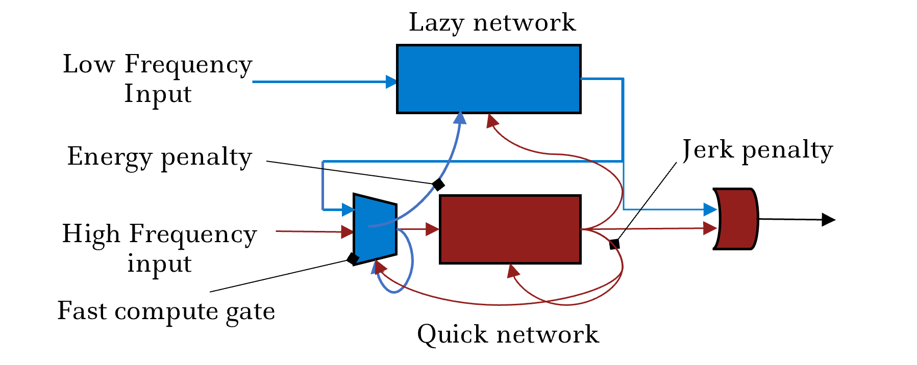
Figure 1: The Temporally Layered Architecture (TLA) comprises two layers: the Lazy layer (blue) and the Quick layer (red). The fast compute gate can activate or deactivate the Quick network. The reward given to each network is augmented differently with the energy and jerk penalty, which forces the overall policy to learn temporal abstractions from performance and energy-based contexts.

Inspired by the biological design, we propose Temporally Layered Architecture (TLA) (Fig. 1): a reinforcement learning architecture that layers two different networks with different frequencies to achieve temporally adaptive behavior. To achieve temporal abstraction, each network has a different constant response frequency - one fast and one slow. The RL agent can use their combination to adapt its response frequency online. The temporally layered architecture allows the agent to easily abstract hierarchical temporal knowledge into layers that focus on different time-frames. We also introduce an energy penalty to aid with temporal abstraction, providing additional context for temporal adaptation and allowing the agent to optimize the dual objectives of accuracy and efficiency. In summary, this work contributes:

1. We propose a bio-inspired Temporally Layered Architecture (TLA), an alternative to classical RL algorithms that allows each layer to focus on a different temporal context.

2. We introduce an algorithm for simultaneously training both layers of TLA that act at different time scales and focus on optimizing for accuracy and energy.

3. We introduce the multi-objective (MOB) score for continuous control tasks to better quantify the quality of policies by combining multiple important metrics for continuous control.

4. We empirically test on a suite of eight continuous control tasks and six different metrics. We demonstrate improved exploration, increased action repetition, lower jerk, fewer decisions, higher action repetition, and lower compute cost (25-80$\%$) on all environments tested. TLA also achieves a higher MOB score on all the environments tested.

2 Related Work

The idea of combining multiple controllers with different response times is, to the best of our knowledge, novel. However, our work is related to several sub-fields of AI reviewed below:

2.1 Continuous Control

Continuous control refers to tasks that involve continuous actions. Compared to discrete control, exploration and learning for continuous control are more difficult and often require a very fast response frequency when using a constant time algorithm.

In this paper, we use the twin-delayed deterministic policy gradient (TD3) method (Fujimoto et al., 2018). TD3 learns two Q-functions (critics) and uses the pessimistic value of the two for training a policy that is updated less frequently than the critics. TD3 is one of the state-of-the-art algorithms for continuous control. However, TLA does not depend on the RL training algorithm and can easily be modified for a different training algorithm.

2.2 Action repetition and frame skipping

Frame-skipping and action repetition have been used as a form of partial open-loop control, where the agent selects a sequence of actions to be executed without considering the intermediate states. Hansen et al. (1996) proposed a mixed-loop control setting, where sensing incurs a cost, thus allowing the agent to perform a sequence of actions to reduce the sensing cost. However, reinforcement learning with a sequence of actions is challenging, since the number of possible action sequences of length $l$ is exponential in $l$. As a result, research in this area focuses on pruning the possible number of actions and states (Hansen et al., 1996; Tan, 1991; McCallum and Ballard, 1996). To avoid the exponential number of action sequences, other works have restricted the action sequences to repeating a single action. The number of actions is, therefore, linear in the number of timesteps (Buckland and Lawrence, 1993; Kalyanakrishnan et al., 2021; Srinivas et al., 2017; Biedenkapp et al., 2021; Sharma et al., 2017). TempoRL, introduced by Biedenkapp et al. (2021), learns an additional action-repetition policy that decides on the number of timesteps to repeat a chosen action. This approach can lead to faster learning and reduce the number of action decision points during an episode. We use their approach as one of our benchmarks.

In their analysis of macro-actions, McGovern et al. (1997) identified two advantages: improved exploration and faster learning due to a reduced task horizon. Empirical evidence from Randløv (1998) also demonstrated that macro-actions significantly reduce training time. Additionally, Braylan et al. (2015) showed that increasing the number of frames skipped can significantly improve the performance of the DQN algorithm Mnih et al. (2015) on some Atari games.

However, these approaches require a predictable environment so that a sequence of actions can be planned and safely performed without supervision. Furthermore, when applied to continuous domains, these approaches often require additional exploration. In contrast, our approach uses a layered architecture, with the faster layer monitoring and acting as required, while the slower layer can be viewed as performing macro-actions.

Recently, Yu et al. (2021) demonstrated a closed-loop temporal abstraction method on the continuous domain using an "act-or-repeat" decision after the action is picked. However, their approach requires two forward passes of the critic in addition to the actor and decision networks, as it uses the state-action value from the critic.

Our approach (TLA) focuses on reducing the number of decisions and compute costs while increasing action repetition compared to previous work.

2.3 Residual and Layered RL

Recently, Jacq et al. (2022) proposed Lazy-MDPs where the RL agent is trained on top of a sub-optimal base policy to act only when needed while deferring the rest of the actions to the base policy. They demonstrated that this approach makes the RL agent more interpretable as the states in which the agent chooses to act are deemed important. Similarly, for continuous environments, residual RL approaches learn a residual policy over a sub-optimal base policy so that the final action is the addition of both actions Silver et al. (2018); Johannink et al. (2019). Residual RL approaches have demonstrated better performance and faster training. Our approach is related to the residual approach, where a faster-frequency network is trained together with a slower-frequency base network to gain the benefits of macro-actions and residual learning. However, unlike the residual approach, the final action for TLA is exclusively picked by a single network. Additionally, residual approaches rely on a pre-trained base policy, while TLA demonstrates that both layers can be trained together.

2.4 Multi-Agent Reinforcement Learning and Non-Stationarity

Multi-agent Reinforcement Learning (MARL) is an open problem with many challenges (Zhang et al., 2021). One of the main difficulties when training multiple agents is dealing with non-stationary environments (Padakandla, 2020). In an environment where multiple agents interact during training, the transition function for each agent is not constant because each agent is learning and updating its policy. As a result, traditional reinforcement learning approaches based on the assumption that the environment can be modeled as a stationary MDP fail to solve MARL tasks.

TLA can be seen as a unique cooperative MARL task in which each agent learns to control the same body together. In cooperative settings, many strategies have been proposed to train agents together (Oroojlooyjadid and Hajinezhad, 2019). However, in our approach, we find that introducing energy constraints induces cooperation and stable learning.

3 Temporally Layered Architecture

In this section, we explore various methods of achieving temporal adaptivity in reinforcement learning. We then introduce a novel architecture and learning algorithm that can learn two distinct temporal abstractions simultaneously and switch between them to optimize both performance and efficiency.

3.1 Temporal Adaptivity

We define temporal adaptivity as the ability to adjust the planning and actuation horizon for control tasks. This adaptivity is necessary to develop time awareness. In many RL tasks, different states require different levels of temporal attention. Some states are unpredictable, resulting in higher entropy for the transition function $p(s_{t+1},a_{t},s_{t})$. In these states, increased supervision is required to ensure that the expected reward does not decrease after the action is taken. In contrast, some states are predictable and have lower entropy for the transition function. In these states, the agent can take more time before sampling input from the environment. The brain takes advantage of this phenomenon by reducing attention in familiar states while increasing it in unfamiliar or unpredictable states. The primary reason for this is to reduce the energy required for computation when it does not affect performance, thus increasing efficiency. However, exploring different temporal scales also has other benefits, as discussed in Section 4.

3.2 Temporally Adaptive Reinforcement Learning

A naive approach to add temporal adaptivity is to treat each action-timestep pair as a different action. The action space is augmented to include the timestep: $\pi:\mathcal{A}=\mathcal{A}\times\mathcal{T}$. However, this is undesirable as it makes the exploration and policy function more complex.

To overcome this issue, many approaches have been proposed that focus on increasing action repetition, as noted in 2.2. Here, we describe two recent approaches that are closest to our approach.

1. TempoRL: In order to reduce the complexity of the problem, Biedenkapp et al. (2021) proposed a setting with two networks: one to select an action and another to determine how long that action should be performed in the environment. However, they do not impose additional constraints or penalties to incentivize longer actions. Additionally, the actions are optimized for a single timestep, so in situations where the optimal extended action differs from the optimal single-step action, TempoRL will not be able to learn the extended action.

2. TAAC: Recently, Yu et al. (2021) demonstrated a closed-loop temporal abstraction method for the continuous domain using an "act-or-repeat" decision after selecting the next action. However, their approach requires two forward passes of the critic (one for the previous action and one for the new action) in addition to the actor at every timestep. This means that while the approach provides closed-loop control with supervision at every timestep, it requires roughly three times more computation than a standard deep RL approach.

3.3 Temporally Layered Architecture (TLA)

To achieve a well-rounded approach to temporal abstraction, we draw inspiration from the brain and biological reflexes, which use multiple layers of computation with different latencies to enable temporal adaptivity. In a similar manner, TLA has two layers, lazy and quick, that learn two policies, each with a different step-size: $\pi_{l}$ and $\pi_{q}$. Where $l$ and $q$ denote the lazy and quick layers, respectively. The $\pi_{q}$ layer is similar to traditional RL agents that observe and act at every timestep, whereas the $\pi_{l}$ layer can only observe and act every $\tau$ timestes, where $\tau\geq 2$ and $\tau\in\mathbb{Z}$.

To switch between these two policies, we also introduce a fast compute gate that decides whether to activate the Quick network based on the state and the lazy action. Therefore, the action at each timestep is:

$$a_{t}=a_{l}\cdot(1-g)+a_{q}\cdot g$$ (1)

Where $a_{l}$ is the lazy action, $a_{q}$ is the quick action, and $g\in\{0,1\}$. Thus, the quick network is activated when $g=1$.

To train both networks simultaneously, experiences are added to the replay memory of both the lazy and the quick networks whenever either network is activated. This is straightforward for the quick network, as it has $\tau$ experiences with the same action created whenever a lazy action is chosen. However, the lazy network can only observe its own actions. To aid training when the quick network is activated, we augment the environmental reward with a jerk penalty as follows:

$$R_{t}=R_{t}-g\cdot((a_{l}-a_{q})/a_{max})\cdot j$$ (2)

Where $j$ is the jerk penalty parameter.

Additionally, the reward of the gate network and the lazy network are augmented with an energy penalty to incentivize lazy actions. Hence, the final rewards for each network are as follows:

$$R^{q}_{t}=R_{t}-g\cdot((a_{l}-a_{q})/a_{max})\cdot j$$ (3)

$$R^{l}_{t}=R_{t}-j\cdot g\cdot(1+((a_{l}-a_{q})/a_{max}))$$ (4)

$$R^{g}_{t}=R_{t}-p\cdot g-g\cdot((a_{l}-a_{q})/a_{max})\cdot j$$ (5)

Here, $p$ is the compute energy penalty parameter. This formulation allows the use of a single hyperparameter $j=p$ for simpler environments with jerk and energy penalties. For multi-dimensional environments that already have an action magnitude penalty, $j$ can be set to zero, and only $p$ needs to be searched. The lazy and quick networks are trained using the TD3 algorithm, while the fast compute gate is trained using Deep Q-learning (Mnih et al., 2015). For completeness, the pseudo-code is presented in the appendix.

4 Experiments

We evaluated TLA on a suite of 8 continuous control environments using the OpenAI gym library (Brockman et al., 2016): two classic control problems and six MuJoCo environments (Todorov et al., 2012). In addition to TLA, we present the TD3 and TempoRL algorithms for each environment as benchmarks. We introduced two new hyperparameters for TLA: the lazy step size $\tau$ and the energy penalty $p$. We set the timestep of the quick-network to be equal to the default step size of the environment. Additionally, for the TempoRL algorithm, the max skip length $J$ was set to be equal to $\tau$, so the longest action repetition possible is the same for both TLA and TempoRL.

The algorithms’ hyperparameters and neural network sizes were kept the same as in previous work (Fujimoto et al., 2018). The maximum training steps for the Pendulum-v1 environment were set to 30,000 and for MountainCarContinuous-v0 were set to 100,000. The rest of the environments were trained until 1,000,000 steps. The initial exploration steps were set to 1,000 for Pendulum-v1, InvertedPendulum-v2, and InvertedDoublePendulum-v2; 10,000 for MountainCarContinuous-v0; and 20,000 for Hopper-v2, Walker2d-v2, Ant-v2, and HalfCheetah-v2. A complete list of hyperparameters is included in the appendix.

For each environment, a hyperparameter search for $\tau$ and $p$ was conducted over 5 random seeds. The final results presented are averaged over 10 random seeds. The hyperparameter search for $\tau$ was limited to a maximum of 11, and $p$ was evaluated over the range [0.1, 6]. Note that for different environments, the average reward per timestep varies, and therefore, the optimal value of $p$ also varies with it. The environments with multidimensional actions (Hopper-v2, Walker2d-v2, Ant-v2, and HalfCheetah-v2) have a control cost included in their rewards, which is similar to the jerk penalty. Thus, for those environments, $j=0$. For the rest of the environments, $j=p$ for simplicity. In the following sections, we evaluate the three algorithms over a variety of metrics important for control tasks.

4.1 Learning speed and Performance

Environment	$\tau$	Normalized AUC			Avg. Return
		TD3	TempoRL	TLA	TD3	TempoRL	TLA
Pendulum	6	0.85	0.85	0.87	-147.38 (29.68)	-149.38 (44.64)	-154.92 (31.97)
MountainCar	11	0.19	0.64	0.82	0(0)	84.56(28.27)	93.88 (0.75)
Inv-Pendulum	10	0.97	0.77	0.96	1000 (0)	984.21 (47.37)	1000(0)
Inv-DPendulum	5	0.96	0.94	0.92	9359.82(0.07)	9352.61(2.20)	9356.67 (1.23)
Hopper	9	0.66	0.43	0.75	3439.12 (120.98)	2607.86 (342.23)	3458.22 (117.92)
Walker2d	7	0.56	0.52	0.53	4223.47 (543.6)	4581.69 (561.95)	3878.41 (493.97)
Ant	3	0.6	0.33	0.52	5131.90(687.00)	3507.85 (579.95)	5163.54 (573.19)
HalfCheetah	3	0.79	0.5	0.58	10352.58 (947.69)	6627.74 (2500.78)	9571.99 (1816.02)

Table 1: Average normalized AUC and average return results. The standard deviation is reported in parentheses. All results are averaged over 10 trials.

Table 1 presents the normalized area under the curve (AUC) and the average return per episode for each algorithm. The speed of convergence can be inferred from both the normalized AUC and the average return. In addition, learning curves for all environments are presented in the appendix. Our results show that TempoRL and TLA have improved exploration, which enhances their learning speed in some environments. This is especially true for the MountainCarContinuous-v0 environment, where exploration using temporally extended actions is necessary to solve the environment.

However, the increased complexity of TempoRL and TLA also hinders their learning speed. For TempoRL, the actions of the skip network increase linearly with the $\tau$ parameter. TLA, on the other hand, introduces non-stationarity to the environments of lazy and gate policies during learning. TLA can be viewed as two agents acting at different frequencies learning a common control task. Like most multi-agent RL tasks, TLA also suffers from non-stationarity: for the same state, the outcome of activating the quick network is different at different points of training. Despite the non-stationarity, TLA achieves similar performance to TD3 on all tasks.

We also note that, although the avg. return of TLA is lower on Pendulum-v1 and Walker2d-v2 environments, the desired behavior is achieved while significantly reducing the number of decisions required, providing a good trade-off between performance and efficiency. Furthermore, Walker2d is well-suited for the TempoRL algorithm, as it requires action repetitions of different lengths for optimal performance. Thus, it is an adversarial environment for TLA, which can only switch between a single action or an action repeated $\tau$ times.

4.2 Action Repetition and Jerk

Environment	$\tau$	Action repetition			Avg. Jerk/timestep
		TD3	TempoRL	TLA	TD3	TempoRL	TLA
Pendulum	6	7.44$\%$	34.94$\%$	70.32$\%$	1.02	0.94	0.62
MountainCar	11	9.08$\%$	75.99$\%$	91.4$\%$	0.1	1.12	1.11
Inv-Pendulum	10	1.12$\%$	45.97$\%$	88.82$\%$	1.11	1.62	0.12
Inv-DPendulum	5	0.95$\%$	14.9$\%$	75.22$\%$	0.1	0.61	0.14
Hopper	9	2.51$\%$	64.99$\%$	57.22$\%$	0.46	0.4	0.25
Walker2d	7	2.14$\%$	69.47$\%$	47.45$\%$	0.27	0.2	0.21
Ant	3	0.82$\%$	22.01$\%$	12.68$\%$	0.43	0.39	0.38
HalfCheetah	3	5.64$\%$	14.07$\%$	18.05$\%$	0.8	0.65	0.67

Table 2: Average action repetition percentage and jerk per timestep. All results are averaged over 10 trials.

In real-world tasks, there is often latency and communication cost involved between action selection and actuation. In such applications, increasing action repetition can reduce the amount of communication required since the same action can be repeated until a new action/directive is received. Therefore, we measure action repetition percentage as the average percentage of timesteps in an episode where the previous action was repeated. For multi-dimensional actions, we calculate action repetition individually over each dimension before averaging, as each action dimension represents a different actuator that requires a separate channel of communication.

Additionally, the single most important metric in continuous control is jerk. The motions of the human body minimize jerk in their behavior to reduce joint stress and energy cost Voros (1999). Thus, it is desirable to reduce jerk in the control task as it reduces energy expended during actuation and reduces the risk of damage or wear to the actuators Tack et al. (2007). We measure jerk as the difference in action magnitude per timestep, as each action represents the torque or force applied. Table 2 shows the action repetition and jerk for all environments. Unsurprisingly, TLA and TempoRL have significantly higher action repetition across all environments and lower jerk across 6 of the eight environments tested. For MountainCar, TD3 does not solve the task and thus, no action results in a lower jerk. For InvertedDoublePendulum-v2, the more fine-grained actions of TD3 allow for a better angle of the pole requiring fewer corrections for balancing, thus lowering the jerk.

TLA also has improved action repetition and jerk over TempoRL for all environments that TempoRL has comparable performance on, except Walker2d. As mentioned in the previous section, Walker2d-v2 is uniquely suited for the TempoRL algorithm.

4.3 Decisions and Compute

Environment	Avg. Decisions			Avg. MMACs			MOB Score
	TD3	TempoRL	TLA	TD3	TempoRL	TLA	TempoRL	TLA
Pendulum	200	139.39	62.31	24.30	34.14	12.42	2.28	9.00
MountainCar	999	116.47	10.6	120.98	28.60	2.54	-	-
Inv-Pendulum	1000	532.57	111.79	121.90	131.01	26.05	-1.13	27.96
Inv-DPendulum	1000	850.95	247.76	124.70	213.59	57.46	-7.36	14.2
Hopper	998.99	269.85	423.91	125.17	68.43	72.02	-13.57	17.44
Walker2d	988.17	297.4	513.12	127.08	77.29	92.07	16.59	12.16
Ant	960.57	741.22	860.21	160.22	248.53	243.22	-2.8	1.45
HalfCheetah	1000	889.57	831.42	128.60	230.13	182.35	-5.91	8.34

Table 3: Average decisions and million multiply-accumulate operations (MMACs) per episode and the multi-objective score for all environments. Decisions and MMACs are averaged over ten trials.

While action repetition and jerk inform us about the cost of actuation, the cost of computation may differ greatly from the decision frequency and the cost of computing the policy. Therefore, we measure the average number of decisions required per episode for each environment. The number of decisions per episode is directly proportional to the compute frequency, so reducing the number of decisions is desirable. This also results in a reduction in compute cost. However, the same number of decisions can result in a significantly different compute cost across different algorithms, as each algorithm has a different number of parameters.

Table 3 shows the average decisions and million multiply-accumulate operations (MMACs) per episode for each task. Unsurprisingly, TLA and TempoRL require significantly fewer decisions than TD3 for every environment tested. However, reduced decisions do not always mean reduced compute costs. Since TempoRL uses two networks for each decision, it requires roughly twice the compute per decision. As a result, TempoRL only reduces the compute cost for three out of the eight environments. By comparison, TLA has three networks and thus roughly three times the number of parameters as TD3. However, since TLA switches between lazy and quick networks, only a fraction of the parameters are used to compute every decision. Due to this, TLA demonstrates significantly lower compute costs (25-80$\%$) on all except two environments that require a higher number of decisions due to the high dimensional action space.

4.4 Multi-Objective Score (MOB)

To compare the qualitative improvement of the continuous control policy over the TD3 benchmark, we introduce the multi-objective score (MOB score). The MOB score is derived by taking the weighted sum of metrics based on their impact on the final policy. The MOB score is defined as follows:

$$MOB=\begin{multlined}(\texttt{perf}_{\texttt{diff}}/\texttt{STD}_{\texttt{TD3}}+0.01\cdot\texttt{perf}_{\texttt{TD3}})^{2}+10\cdot N_{\texttt{actuators}}\cdot\texttt{jerk}_{\texttt{diff}}+\\ 0.01\cdot\texttt{AR}_{\texttt{diff}}+0.05\cdot\texttt{decisions}_{\texttt{diff}}+0.05\cdot\texttt{MMAC}_{\texttt{diff}}\end{multlined}(\texttt{perf}_{\texttt{diff}}/\texttt{STD}_{\texttt{TD3}}+0.01\cdot\texttt{perf}_{\texttt{TD3}})^{2}+10\cdot N_{\texttt{actuators}}\cdot\texttt{jerk}_{\texttt{diff}}+\\ 0.01\cdot\texttt{AR}_{\texttt{diff}}+0.05\cdot\texttt{decisions}_{\texttt{diff}}+0.05\cdot\texttt{MMAC}_{\texttt{diff}}$$ (6)

The MOB score measures how good a policy is when compared to the TD3 benchmark. It rewards or penalizes large differences in performance. After performance, the focus should be on energy minimization. Since actuation cost is the highest energy cost, we weight jerk the most (scaled for the number of actuators), followed by the MMACs for compute cost. Communication costs are represented by action repetition and decisions, which have lower weightage. MOB scores for TLA and TempoRL are presented in Table 3. TLA shows an improved MOB score in all environments except Ant-v2, while TempoRL only shows an improvement in two environments. The MOB score weights can be easily modified for applications with different constraints. Additionally, the TD3 benchmark can be replaced with any constant frequency algorithm for comparison.

Furthermore, when designing AI for control that interacts with humans, it is important that the AI behaves in a natural and human-like manner (Zuniga et al., 2022). We believe that optimizing for energy automatically leads to natural behavior. Videos demonstrating this can be found in the appendix. A formal qualitative study is left for future work.

4.5 Impact of choice of step-size and penalties (sweet-spot)

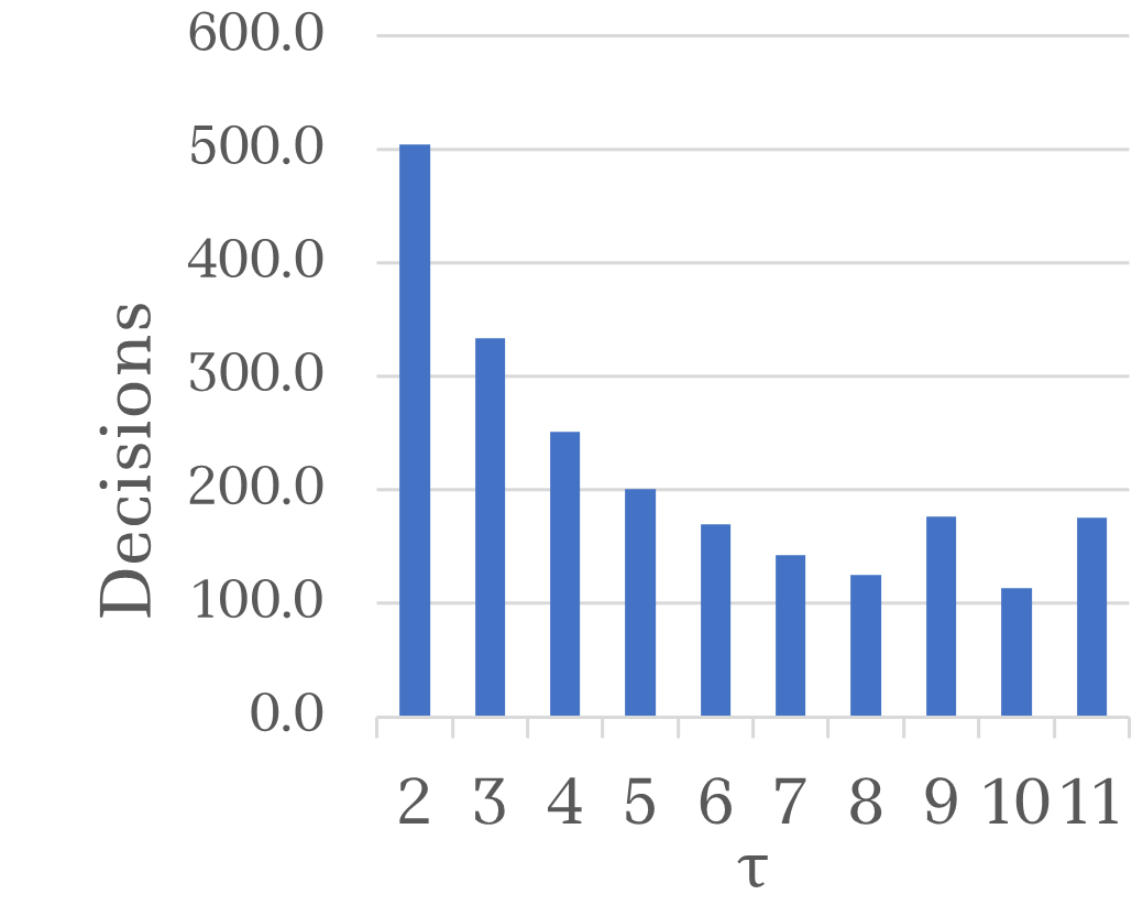
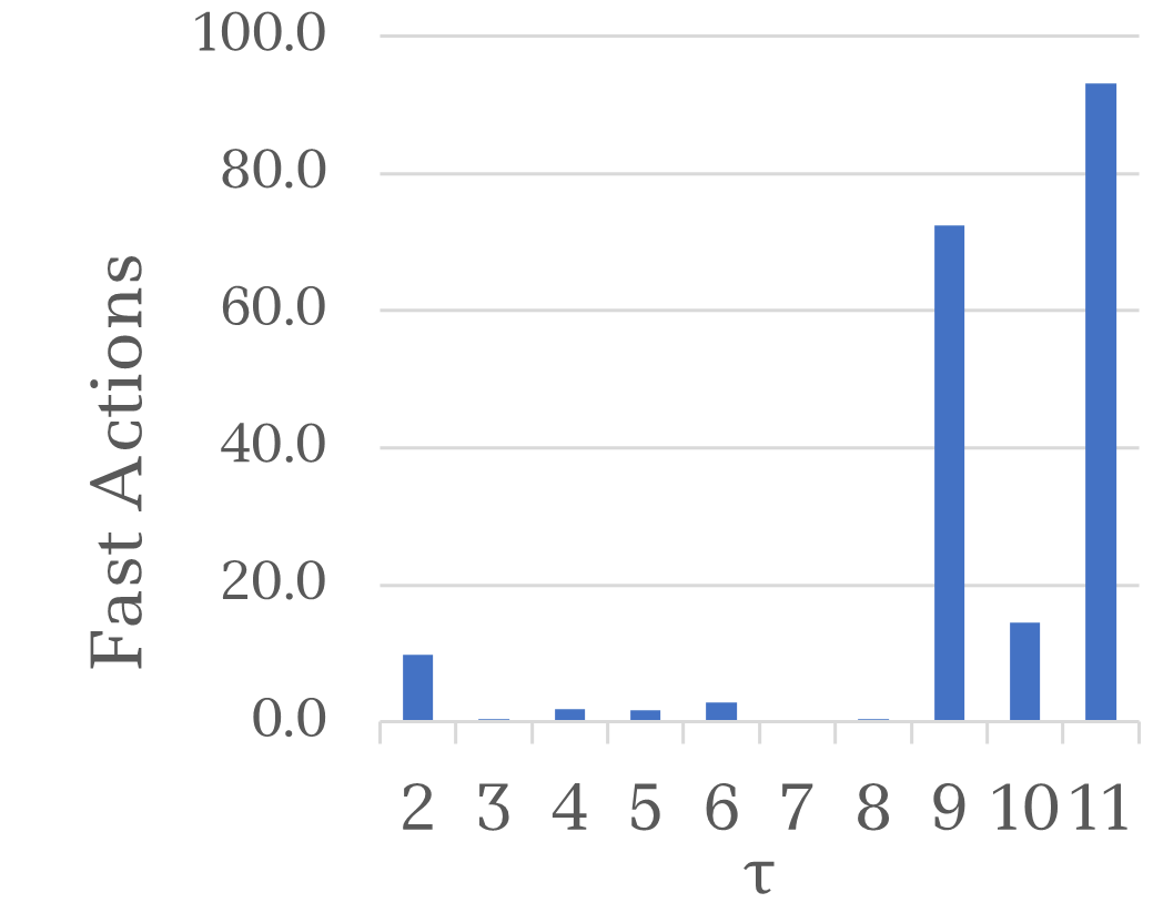
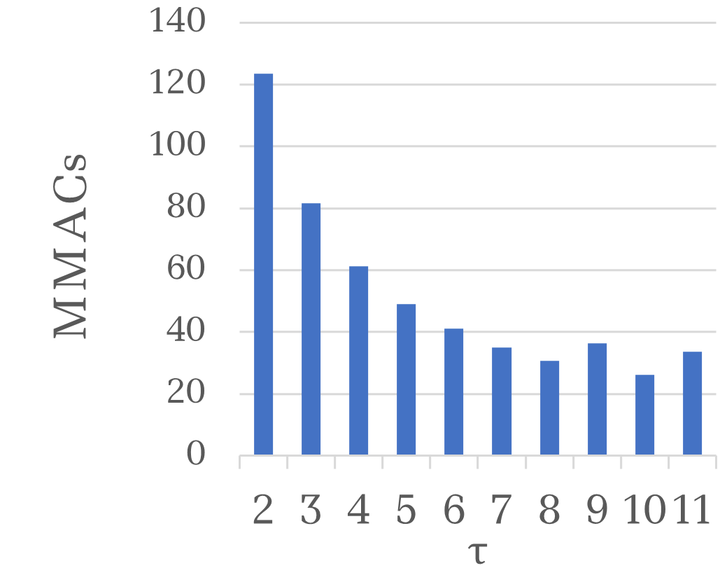
Figure 2: Effect of $\tau$ on the number of decisions, quick actions and MMACs for InvertedPendulum-v2 environment.

The choice of step-size $\tau$ significantly affects the decisions and compute cost of TLA. If the lazy layer becomes slower, the number of decisions and compute cost is reduced. However, if the lazy layer is too slow, the quick layer needs to intervene more often, resulting in an increase in compute. This phenomenon results in a sweet spot of step size that allows for the lowest possible compute cost and decisions. Figure 2 demonstrates this effect on the InvertedPendulum-v2 environment. A similar behavior is observed in the brain, which operates at two different frequencies: one for planning and one for fast reactions Nakahira et al. (2021).

Similarly, the choice of the penalty $p$ impacts the number of decisions as a higher $p$ reduces the number of quick actions taken. Curiously, the penalty also enables learning for TLA by providing an additional energy constraint. When the penalty is too low, TLA fails to learn, suggesting that the penalty alleviates the problem of non-stationarity in TLA. The results on the impact of the energy penalty are included in the appendix.

5 Limitations and Future work

The main limitation of TLA is that it can only plan a sequence of actions consisting of a single action. Therefore, the benefits of TLA are reduced in multidimensional actions. In the future, we plan to implement a lazy layer that can plan a sequence of actions instead of repeating the same action. In TLA, the quick layer acts as a reflex that only activates when needed, while the lazy layer acts as a planning network in the brain. However, even within the brain, temporal attention is adaptable (Morillon et al., 2016). Thus, in the future, we will also explore making the step size of the lazy layer adaptable to allow for changes in the planning horizon, while the quick network only acts in unexpected situations. This will especially lead to improvements in the Walker2d environment.

6 Conclusion

We introduced Temporally Layered Architecture (TLA) for continuous control, which demonstrates a better control policy than state-of-the-art reinforcement learning (RL) algorithms across multiple relevant metrics. The TLA takes inspiration from the brain and adapts its action frequency by switching between a lazy policy, with less supervision and higher efficiency, and a quick policy that provides increased supervision at the cost of compute. Control algorithms should not only optimize for performance, but also focus on multiple objectives to achieve better performance. To that end, we empirically evaluated our method against existing approaches and demonstrated that the same performance can be achieved with 25-80$\%$ lower compute cost. Additionally, we demonstrate that optimizing the twin objectives of performance and energy results in reduced jerk and increased action repetition, resulting in more natural control. Finally, we propose the MOB score, a robust benchmark with multiple metrics for future work on continuous control tasks.

The numerous benefits of TLA make it suitable for use in energy-constrained environments, environments that require a distributed approach, and environments with high communication costs or delays. In the future, we plan to improve TLA by allowing the lazy layer to plan a sequence of different actions, thus reducing compute and improving performance even further.

References

- Biedenkapp et al. (2021) A. Biedenkapp, R. Rajan, F. Hutter, and M. T. Lindauer. Temporl: Learning when to act. In ICML, 2021.
- Braylan et al. (2015) A. Braylan, M. Hollenbeck, E. Meyerson, and R. Miikkulainen. Frame skip is a powerful parameter for learning to play atari. In AAAI Workshop: Learning for General Competency in Video Games, 2015.
- Brockman et al. (2016) G. Brockman, V. Cheung, L. Pettersson, J. Schneider, J. Schulman, J. Tang, and W. Zaremba. Openai gym, 2016.
- Buckland and Lawrence (1993) K. M. Buckland and P. D. Lawrence. Transition point dynamic programming. In NIPS, 1993.
- Fujimoto et al. (2018) S. Fujimoto, H. van Hoof, and D. Meger. Addressing function approximation error in actor-critic methods. ArXiv, abs/1802.09477, 2018.
- Haarnoja et al. (2018) T. Haarnoja, A. Zhou, P. Abbeel, and S. Levine. Soft actor-critic: Off-policy maximum entropy deep reinforcement learning with a stochastic actor. In International conference on machine learning, pages 1861–1870. PMLR, 2018.
- Hansen et al. (1996) E. A. Hansen, A. G. Barto, and S. Zilberstein. Reinforcement learning for mixed open-loop and closed-loop control. In NIPS, 1996.
- Heitz (2014) R. P. Heitz. The speed-accuracy tradeoff: history, physiology, methodology, and behavior. Frontiers in neuroscience, 8:150, 2014.
- Jacq et al. (2022) A. Jacq, J. Ferret, O. Pietquin, and M. Geist. Lazy-mdps: Towards interpretable reinforcement learning by learning when to act. ArXiv, abs/2203.08542, 2022.
- Johannink et al. (2019) T. Johannink, S. Bahl, A. Nair, J. Luo, A. Kumar, M. Loskyll, J. A. Ojea, E. Solowjow, and S. Levine. Residual reinforcement learning for robot control. 2019 International Conference on Robotics and Automation (ICRA), pages 6023–6029, 2019.
- Kalyanakrishnan et al. (2021) S. Kalyanakrishnan, S. Aravindan, V. Bagdawat, V. Bhatt, H. Goka, A. Gupta, K. Krishna, and V. Piratla. An analysis of frame-skipping in reinforcement learning. ArXiv, abs/2102.03718, 2021.
- McCallum and Ballard (1996) A. McCallum and D. H. Ballard. Reinforcement learning with selective perception and hidden state. 1996.
- McGovern et al. (1997) A. McGovern, R. S. Sutton, and A. H. Fagg. Roles of macro-actions in accelerating reinforcement learning. 1997.
- Mnih et al. (2015) V. Mnih, K. Kavukcuoglu, D. Silver, A. A. Rusu, J. Veness, M. G. Bellemare, A. Graves, M. A. Riedmiller, A. Fidjeland, G. Ostrovski, S. Petersen, C. Beattie, A. Sadik, I. Antonoglou, H. King, D. Kumaran, D. Wierstra, S. Legg, and D. Hassabis. Human-level control through deep reinforcement learning. Nature, 518:529–533, 2015.
- Moore (1990) A. W. Moore. Efficient memory-based learning for robot control. Technical report, University of Cambridge, 1990.
- Morillon et al. (2016) B. Morillon, C. E. Schroeder, V. Wyart, and L. H. Arnal. Temporal prediction in lieu of periodic stimulation. The Journal of Neuroscience, 36:2342 – 2347, 2016.
- Nakahira et al. (2021) Y. Nakahira, Q. Liu, T. J. Sejnowski, and J. C. Doyle. Diversity-enabled sweet spots in layered architectures and speed–accuracy trade-offs in sensorimotor control. Proceedings of the National Academy of Sciences, 118, 2021.
- Nobre (2001) A. C. Nobre. Orienting attention to instants in time. Neuropsychologia, 39:1317–1328, 2001.
- Nobre and van Ede (2018) A. C. Nobre and F. van Ede. Anticipated moments: temporal structure in attention. Nature Reviews Neuroscience, 19:34–48, 2018.
- Oroojlooyjadid and Hajinezhad (2019) A. Oroojlooyjadid and D. Hajinezhad. A review of cooperative multi-agent deep reinforcement learning. ArXiv, abs/1908.03963, 2019.
- Padakandla (2020) S. Padakandla. A survey of reinforcement learning algorithms for dynamically varying environments. ACM Computing Surveys (CSUR), 54:1 – 25, 2020.
- Randløv (1998) J. Randløv. Learning macro-actions in reinforcement learning. In NIPS, 1998.
- Sharma et al. (2017) S. Sharma, A. Srinivas, and B. Ravindran. Learning to repeat: Fine grained action repetition for deep reinforcement learning. ArXiv, abs/1702.06054, 2017.
- Silver et al. (2018) T. Silver, K. R. Allen, J. B. Tenenbaum, and L. P. Kaelbling. Residual policy learning. ArXiv, abs/1812.06298, 2018.
- Srinivas et al. (2017) A. Srinivas, S. Sharma, and B. Ravindran. Dynamic action repetition for deep reinforcement learning. In AAAI, 2017.
- Tack et al. (2007) G.-R. Tack, J. Choi, J. Yi, and C. Kim. Relationship between jerk cost function and energy consumption during walking. In World Congress on Medical Physics and Biomedical Engineering 2006: August 27–September 1, 2006 COEX Seoul, Korea “Imaging the Future Medicine”, pages 2917–2918. Springer, 2007.
- Tan (1991) M. Tan. Cost-sensitive reinforcement learning for adaptive classification and control. In AAAI, 1991.
- Todorov et al. (2012) E. Todorov, T. Erez, and Y. Tassa. Mujoco: A physics engine for model-based control. In 2012 IEEE/RSJ International Conference on Intelligent Robots and Systems, pages 5026–5033. IEEE, 2012. doi: 10.1109/IROS.2012.6386109.
- Voros (1999) T. Voros. Minimum jerk theory revisited. In Proceedings of the First Joint BMES/EMBS Conference. 1999 IEEE Engineering in Medicine and Biology 21st Annual Conference and the 1999 Annual Fall Meeting of the Biomedical Engineering Society (Cat. N, volume 1, pages 532 vol.1–, 1999. doi: 10.1109/IEMBS.1999.802610.
- Yu et al. (2021) H. Yu, W. Xu, and H. Zhang. Taac: Temporally abstract actor-critic for continuous control. In NeurIPS, 2021.
- Zhang et al. (2021) K. Zhang, Z. Yang, and T. Başar. Multi-agent reinforcement learning: A selective overview of theories and algorithms. Handbook of reinforcement learning and control, pages 321–384, 2021.
- Zuniga et al. (2022) E. Zuniga, S. Milani, G. Leroy, J. Rzepecki, R. Georgescu, I. Momennejad, D. Bignell, M. Sun, A. Shaw, G. Costello, et al. How humans perceive human-like behavior in video game navigation. In CHI Conference on Human Factors in Computing Systems Extended Abstracts, pages 1–11, 2022.