Approximation and Estimation Ability of Transformers
for Sequence-to-Sequence Functions with Infinite Dimensional Input

Abstract

Despite the great success of Transformer networks in various applications such as natural language processing and computer vision, their theoretical aspects are not well understood. In this paper, we study the approximation and estimation ability of Transformers as sequence-to-sequence functions with infinite dimensional inputs. Although inputs and outputs are both infinite dimensional, we show that when the target function has anisotropic smoothness, Transformers can avoid the curse of dimensionality due to their feature extraction ability and parameter sharing property. In addition, we show that even if the smoothness changes depending on each input, Transformers can estimate the importance of features for each input and extract important features dynamically. Then, we proved that Transformers achieve similar convergence rate as in the case of the fixed smoothness. Our theoretical results support the practical success of Transformers for high dimensional data.

1 Introduction

Transformer networks, first proposed in Vaswani et al. (2017), empirically show high performance in various fields including natural language processing (Vaswani et al., 2017), computer vision (Dosovitskiy et al., 2021) and audio processing (Dong et al., 2018), where the dimensionality of inputs is relatively high. However, despite the growing interest in Transformer models, their theoretical properties are still unclear.

Aside from the Transformer architecture, there exists a line of work which studied the approximation and estimation ability of fully connected neural networks (FNN) for certain function spaces such as Hölder spaces (Schmidt-Hieber, 2020) and Besov spaces (Suzuki, 2018). For example, Schmidt-Hieber (2020) showed that FNNs with ReLU activation can achieve the near minimax optimal rate of the estimation error for composite functions in Hölder spaces. Although deep learning can achieve the near optimal rate for several function classes, the convergence rate is often strongly affected by the dimensionality of inputs. Some researches (Nakada & Imaizumi, 2022; Chen et al., 2022) considered the settings where the data are distributed on a low dimensional manifold and showed that deep neural networks can avoid the curse of dimensionality. However, this assumption is relatively strong since the low dimensionality of the data manifold is easily destroyed by noise injection. Then, Suzuki (2018) showed that even if the data manifold is not low dimensional, deep neural networks can avoid the curse of dimensionality under the assumption that the target function has anisotropic smoothness. Moreover, Okumoto & Suzuki (2022) showed that (dilated) convolutional neural networks (CNN) can avoid the curse of dimensionality even if inputs are infinite dimensional.

Although the learnability of FNNs and CNNs has been intensively studied, that of Transformer networks is not well understood. There are some researches (Edelman et al., 2022; Gurevych et al., 2022) which studied the learning ability of Transformers. Edelman et al. (2022) evaluated the capacity of Transformer networks and derived the sample complexity to learn sparse Boolean functions. Since they investigated discrete inputs, the smoothness of the target function was not considered. Gurevych et al. (2022) studied binary classification tasks and proved that Transformer networks can avoid the curse of dimensionality when a posteriori probability is represented by the hierarchical composition model with Hölder smoothness. However, these studies have some limitations. First, the previous works considered the fixed length input, although Transformer networks can be applied to sequences of any length due to the parameter sharing property, even if the length is infinite. Indeed, Transformers are often applied to very high dimensional data such as images and languages, and the learnability of Transformers for such extremely high dimensional data is still unclear. Second, their analysis is limited to the single output setting. In some applications such as question-answering, it is necessary to learn a function that maps an input sequence to an output sequence. Transformer networks can be applied to such situations and achieve great practical success as represented by BERT (Devlin et al., 2019) although output is also high dimensional. Finally, in these studies, the intrinsic structure of target functions does not depend on each input and the pattern of attention weights does not change. This is in contrast to the dynamic nature of self-attention matrices observed in practice (Likhosherstov et al., 2021).

In this paper, we consider the non-parametric regression problems and study the approximation and estimation ability of Transformers for sequence-to-sequence functions with infinite dimensional inputs. In the high dimensional setting, the dependence of the target function on inputs varies depending on the direction. For example, in image classification, the target function is more dependent on foreground features than background features. To deal with such situations, we consider direction-dependent smoothness. Then, we derive the convergence rate of errors for mixed and anisotropic smooth functions and show that Transformer networks can avoid the curse of dimensionality. In addition, we consider the setting where the position of important features changes depending on each input and show that Transformer networks can avoid the curse of dimensionality, which reveals the dynamical feature extraction ability of self-attention mechanism. Our contribution can be summarized as follows.

• We derive the convergence rate of approximation and estimation error for shift-equivariant functions with the mixed or anisotropic smoothness. We show that the errors are dependent only on the smoothness of the target function and independent of the input and output dimension. This means that Transformers can avoid the curse of dimensionality even if the dimensionality of inputs and outputs is infinite.

• We consider the situation where the smoothness of each coordinate, which corresponds to the importance of each feature, changes depending on inputs and derive the similar convergence rate to the case of the fixed smoothness.

1.1 Other Related Works

Yun et al. (2020); Zaheer et al. (2020) proved that Transformers with learnable positional encodings are universal approximators of continuous sequence-to-sequence functions with compact support, but the results suffer from the curse of dimensionality. This is unavoidable as mentioned in Yun et al. (2020). To derive meaningful convergence results, it is necessary to restrict the function class. From this perspective, Edelman et al. (2022) investigated sparse Boolean functions and Gurevych et al. (2022) studied the hierarchical composition model. However, our analysis imposes smoothness structure on target functions more directly compared to these studies.

The mixed and anisotropic smooth function spaces which we consider in this study are extensions of the functions investigated in Okumoto & Suzuki (2022). In addition, the function spaces can be seen as an infinite dimensional counterpart of the mixed Besov space (Schmeisser, 1987) and anisotropic Besov space (Nikol’skii, 1975). From the deep learning perspective, the approximation and estimation error of FNNs for the mixed Besov space and anisotropic Besov space was analyzed in Suzuki (2018) and Suzuki & Nitanda (2021), respectively. However, it is not trivial to extend these results to Transformer architecture and multiple output setting.

In this paper, we also consider the piecewise $\gamma$-smooth function class. This function class is inspired by the piecewise smooth functions, which was investigated in Petersen & Voigtlaender (2018); Imaizumi & Fukumizu (2019), but these studies did not consider anisotropic smoothness and Transformer networks.

There are some studies that investigated the theoretical properties of Transformer networks from different perspective than ours. Jelassi et al. (2022) analyzed simplified Vision transformers and showed that they can learn the spatial structure via gradient descent. Zhang et al. (2022) studied the self-attention mechanism from the perspective of exchangeability and proved that Transformer networks can learn desirable representation of input tokens. Pérez et al. (2019) showed the Turing completeness of Transformers and Wei et al. (2021) introduced the notion of statistically meaningful approximation and gave the sample complexity to approximate Boolean circuits and Turing machines. Likhosherstov et al. (2021) showed that a self-attention module with fixed parameters can approximate any sparse matrix by designing an input appropriately.

1.2 Notations

Here, we prepare the notations. For $l\in\mathbb{N}$, let $[l]$ be the set $\quantity{1,\dots,l}$ and for $l,r\in\mathbb{Z}~{}(l\leq r)$, let $[l:r]$ be the set $\quantity{l,\dots,r}$. For a set $\mathbb{S}\subset\mathbb{R}$ and $d\in\mathbb{N}$, let

$$\mathbb{S}^{d\times\infty} :=\quantity{[\dots,s_{-1},s_{0},s_{1},\dots,s_{i},\dots]\mid s_{i}\in\mathbb{S}^{d}},$$

$$\mathbb{S}_{0}^{d\times\infty} :=\quantity{s\in(\mathbb{S}\cup\quantity{0})^{d\times\infty}\mid\absolutevalue{\operatorname{supp}(s)}<\infty},$$

where $\operatorname{supp}(s)$ is defined as $\quantity{(i,j)\in[d]\times\mathbb{Z}\mid s_{i,j}\neq 0}$. Similary, $\mathbb{S}^{d\times[l:r]}$ denotes the set $\quantity{[s_{l},\dots s_{r}]\mid s_{j}\in\mathbb{S}}$. For $X=[\dots,x_{0},x_{1},\dots]\in\mathbb{R}^{d\times\infty}$, $X[l:r]$ denotes $[x_{l},\dots,x_{r}]\in\mathbb{R}^{d\times[l:r]}$. For $s\in\mathbb{R}_{0}^{d\times\infty}$, let $2^{s}:=2^{\sum_{i\in[d],j\in\mathbb{Z}}s_{ij}}$. For $X\in\mathbb{R}^{d\times\infty}$, $\norm{X}_{\infty}$ denotes $\sup_{i\in[d],j\in\mathbb{Z}}\absolutevalue{X_{i,j}}$ and for $x\in\mathbb{R}^{l}$, $\norm{x}_{1}$ denotes $\sum_{i=1}^{l}\absolutevalue{x_{i}}$. For $F:\Omega\to\mathbb{R}^{l}$, let $\norm{F}_{\infty}:=\sup_{X\in\Omega}\norm{F(X)}_{\infty}$. For the probability measure $P_{X}$ on $\Omega$ and $p>0$, the norm $\norm{\cdot}_{p,P_{X}}$ is defined by

$$\norm{f}_{p,P_{X}} =\quantity(\int_{\Omega}\norm{f(X)}_{p}^{p}\differential{P_{X}})^{1/p}.$$

For a matrix $A$, let $\norm{A}_{0}=\absolutevalue{\quantity{(i,j)\mid A_{ij}\neq 0}}$. For $j\in\mathbb{Z}$, we define the shift operator $\Sigma_{j}:\mathbb{R}^{d\times\infty}\to\mathbb{R}^{d\times\infty}$ by $(\Sigma_{j}(X))_{i}=x_{i+j}$ for $X=[\dots,x_{0},\dots,x_{i},\dots]\in\mathbb{R}^{d\times\infty}$. For a normed space $\mathcal{F}$, we define $U(\mathcal{F})$ by $U(\mathcal{F}):=\quantity{f\in\mathcal{F}\mid\norm{f}_{\mathcal{F}}\leq 1}$, where $\norm{\cdot}_{\mathcal{F}}$ is the norm of $\mathcal{F}$.

2 Problem Settings

2.1 Non-parametric Regression Problems

In this paper, we consider non-parametric regression problems with infinite dimensional inputs. We regard an input $X\in[0,1]^{d\times\infty}$ as a bidirectional sequence of tokens $\quantity{x_{i}}_{i=-\infty}^{\infty}~{}(x_{i}\in\mathbb{R}^{d})$. For example, each token $x_{i}$ corresponds to a word vector in natural language processing and an image patch in image processing (Dosovitskiy et al., 2021). Let $P_{X}$ be a probability measure on $([0,1]^{d\times\infty},\mathcal{B}([0,1]^{d\times\infty}))$. We write $\Omega$ for the support of $P_{X}$. We assume that $P_{X}$ is shift-invariant. That is, for any $i\in\mathbb{Z}$ and $B\in\mathcal{B}([0,1]^{d\times\infty})$, $P_{X}(B)=P_{X}(\quantity{\Sigma_{i}(X)\mid X\in B})$. In the non-parametric regression, we observe $n$ i.i.d. pairs of inputs $X^{(i)}\sim P_{X}$ and outputs $Y^{(i)}\in\mathbb{R}^{\infty}$. We assume that there exists a true function $F^{\circ}:\Omega\to\mathbb{R}^{\infty}$, and outputs $Y^{(i)}$ is given by

$$Y^{(i)} :=F^{\circ}(X^{(i)})+\xi^{(i)},$$

where the noise $\xi^{(i)}_{j}$ follows the normal distribution $N(0,\sigma^{2})~{}(\sigma>0)$ independently. We also assume that $\quantity{\xi^{(i)}}_{i=1}^{n}$ are independent of $\quantity{X^{(i)}}_{i=1}^{n}$. Note that unlike Okumoto & Suzuki (2022), we do not assume that the Radon-Nikodym derivative $\frac{\differential{P_{X}}}{\differential{\lambda}}$ for the uniform distribution $\lambda$ on $([0,1]^{d\times\infty},\mathcal{B}([0,1]^{d\times\infty}))$ satisfies $\norm{\frac{\differential{P_{X}}}{\differential{\lambda}}}_{\infty}<\infty$.

Based on the observed data $\mathcal{D}^{n}:=\quantity{(X^{(i)},Y^{(i)})}_{i=1}^{n}$, we compute an estimator $\hat{F}$ which takes its value in the class of Transformer networks. To evaluate the statistical performance of an estimator $\hat{F}$, we consider the mean squared error

$$R_{l,r}(\hat{F},F^{\circ})=\frac{1}{r-l+1}\sum_{i=l}^{r}\mathbb{E}\quantity[\norm{\hat{F}_{i}-F^{\circ}_{i}}_{2,P_{X}}^{2}],$$

where the expectation is taken with respect to the training data $\mathcal{D}^{n}$. Here, to avoid the convergence argument, we consider a finite number of outputs ($Y^{(i)}_{l},\dots,Y^{(i)}_{r}$), but we show later that the convergence rate of estimation error does not depend on $l$ and $r$.

In this paper, we consider an empirical risk minimization (ERM) estimator, which is defined as a minimizer of the following minimization problem:

$$\min_{F\in\mathcal{T}}\sum_{i=1}^{n}\sum_{j=l}^{r}\quantity(F(X^{(i)})_{j}-Y^{(i)}_{j})^{2},$$

where $\mathcal{T}$ is supposed to be the set of Transformer networks defined in Eq. (1). Note that an ERM estimator $\hat{F}$ is a random variable which depends on the training dataset $\mathcal{D}^{n}$. In practice, it is difficult to solve the problem due to the non-convexity of the objective function. Some studies (Huang et al., 2020; Jelassi et al., 2022) investigated the optimization aspect of Transformers, but we do not pursue this direction in this study.

2.2 Transformer Architecture

Transformer architecture has three main components:

1. (position-wise) FNN layer.

2. Self-attention layer.

3. Embedding layer.

(i) First, we introduce FNN layers. An FNN with depth $L$ and width $W$ is defined as

$$f(x):=(A_{L}\eta(\cdot)+b_{L})\circ\dots\circ(A_{1}x+b_{1}),$$

where $A_{i}\in\mathbb{R}^{d_{i+1}\times d_{i}},b_{i}\in\mathbb{R}^{d_{i+1}}$, $\max_{i}d_{i}\leq W$, and ReLU activation function $\eta(x)=\max\quantity{x,0}$ is operated in an element-wise manner. Then, we define the class of FNN with depth $L$, width $W$, norm bound $B$ and sparsity $S$ by

$$\Psi(L,W,S,B):= \left\{f\mid\max_{i}\quantity{\norm{A_{i}}_{\infty},\norm{b_{i}}_{\infty}}\leq B,\right.$$

$$\quad\left.\sum_{i=1}^{L}\norm{A_{i}}_{0}+\norm{b_{i}}_{0}\leq S\right\}.$$

(ii) Next, we define the self-attention layer. In this paper, we consider the sliding window attention, which is used in some practical architectures such as Longformer (Beltagy et al., 2020) and Big Bird (Zaheer et al., 2020). To focus on local context, the sliding window attention restricts the receptive field to the input around each token. Let $D$ be the embedding dimension, $H$ be the number of head, and $U$ be the window size. Then, self-attention layer $g$ with parameters $K_{h}\in\mathbb{R}^{D^{\prime}\times D},Q_{h}\in\mathbb{R}^{D^{\prime}\times D},V_{h}\in\mathbb{R}^{D\times D}~{}(D^{\prime}\leq D,h=1,\dots,H)$ is defined by

$$g(X)_{i} :=x_{i}+\sum_{h=1}^{H}V_{h}X[i-U:i+U]A_{h},$$

where

$$A_{h} :=\operatorname{Softmax}((K^{(h)}X[i-U:i+U])^{\top}(Q^{(h)}x_{i})),$$

$$\in\mathbb{R}^{[i-U:i+U]}.$$

Here, $\operatorname{Softmax}:\mathbb{R}^{l}\to\mathbb{R}^{l}$ is defined by

$$\operatorname{Softmax}(x)=\quantity[\frac{e^{x_{1}}}{\sum\limits_{j\in[l]}e^{x_{j}}},\dots,\frac{e^{x_{l}}}{\sum\limits_{j\in[l]}e^{x_{j}}}]^{\top}.$$

Then, we define the class of self-attention layers with the window size $U\in\mathbb{N}$, the embedding dimension $D$, the number of head $H$, and the norm bound $B$ by

$$\mathcal{A}(U,D,H,B)$$

$$\quad:=\quantity{g\mid\max_{h}\quantity{\norm*{K_{h}}_{\infty},\norm*{Q_{h}}_{\infty},\norm*{V_{h}}_{\infty}}\leq B}.$$

(iii) Finally, we define the embedding layer. For embedding dimension $D$, an embedding layer is defined as

$$\operatorname{Enc}_{P}(X) =EX+P,$$

where $E\in\mathbb{R}^{D\times d},~{}P=[p_{i}]_{i=-\infty}^{\infty}\in\mathbb{R}^{D\times\infty}$. Here, $P$ is called a positional encoding. Since position-wise FNN and self-attention layers are permutation equivariant, a positional encoding is often added to break the equivariance when positional information is important. Sometimes, a learnable positional encoding is used, but we consider that $P$ is fixed since $P$ is infinite dimensional in our setting. Relative positional encoding (Shaw et al., 2018) is another way to encode the positional information, but it requires extra trainable parameters. Therefore, we consider the absolute positional encoding in this paper.

We define the class of transformers by

$$\mathcal{T}(M,U,D,H,L,W,S,B)$$

$$\quad:=\left\{f_{M}\circ g_{M}\circ\dots\circ f_{1}\circ g_{1}\circ\operatorname{Enc}_{P}\mid\norm{E}_{\infty}\leq B,\right.$$

$$\quad\left.f_{i}\in\Psi(L,W,S,B),g_{i}\in\mathcal{A}(U_{i},D,H,B)\right\},$$

where FNN is applied column-wise. Thanks to the parameter sharing property, $F\in\mathcal{T}$ can represent a function from $[0,1]^{d\times\infty}$ to $\mathbb{R}^{\infty}$ even though it has a finite number of parameters. In order to derive the estimation error for a model class $\mathcal{T}$, it is convenient to assume that there exists a constant $R>0$ such that $\norm{f}_{\infty}\leq R$ for any $f\in\mathcal{F}$ since this assumption ensure the sub-Gaussianity of $f(X^{(i)})$. To ensure this property, we define the class of (clipped) Transformer networks by

$$\mathcal{T}_{R}:=\quantity{\tilde{F}=\operatorname{clip}_{R}\circ F\mid F\in\mathcal{T}},$$ (1)

where $\operatorname{clip}_{R}(x):=R\wedge(x\vee-R)$ is applied element-wise. Note that $\operatorname{clip}_{R}$ can be realized by ReLU units.

For simplicity, we consider a modified version of the original architecture in Vaswani et al. (2017). That is, we consider the multilayer FNNs without skip connection instead of the single layer FNNs with skip connection. However, our argument can be applied to the original architecture with a slight modification. See Appendix B for details.

3 Function Spaces

In this paper, we assume the true function $F^{\circ}$ is shift-equivariant. A function $F:\Omega\to\mathbb{R}^{d^{\prime}\times\infty}$ is called shift-equivariant if $F$ satisfies

$$F(\Sigma_{j}(X))=\Sigma_{j}(F(X)),$$

for any $j\in\mathbb{Z}$ and $X\in\Omega$. Such equivariance appears in various applications such as natural language processing, audio processing, and time-series analysis. We also assume that $F_{i}(X):=(F(X))_{i}$ is included in a certain function class which is defined in this section.

3.1 Anisotropic and Mixed Smoothness

First, we introduce the $\gamma$-smooth function class. This is an extension of the function class in Okumoto & Suzuki (2022) to the situation where the inputs are bidirectional sequences of tokens. For $r\in\mathbb{Z}_{0}^{d\times\infty}$, we define $\psi_{r_{ij}}:[0,1]\to\mathbb{R}$ by

$$\psi_{r_{ij}}(x) :=\begin{cases}\sqrt{2}\cos(2\pi\absolutevalue{r_{ij}}x)&\quad(r_{ij}<0),\\ 1&\quad(r_{ij}=0),\\ \sqrt{2}\sin(2\pi\absolutevalue{r_{ij}}x)&\quad(r_{ij}>0),\end{cases}$$

and $\psi_{r}:[0,1]^{d\times\infty}\to\mathbb{R}$ by $\psi_{r}(X)=\prod_{i=1}\prod_{j=1}\psi_{r_{ij}}(X_{ij})$. Since $\quantity{\psi_{r}}_{r\in\mathbb{Z}_{0}^{d\times\infty}}$ is a complete orthonormal system of $L^{2}([0,1]^{d\times\infty})$, any $f\in L^{2}([0,1]^{d\times\infty})$ can be expanded as $f=\sum_{r\in\mathbb{Z}_{0}^{d\times\infty}}\expectationvalue{f,\psi_{r}}\psi_{r}$. For $s\in\mathbb{N}_{0}^{d\times\infty}$, define $\delta_{s}(f)$ as

$$\delta_{s}(f)=\sum_{r\in\mathbb{Z}_{0}^{d\times\infty},\lfloor 2^{{s_{ij}-1}}\rfloor\leq r_{ij}<2^{s_{ij}}}\expectationvalue{f,\psi_{r}}\psi_{r}.$$

This quantity represents the frequency component of $f$ with frequency $\absolutevalue{r_{ij}}\sim 2^{s_{ij}}$ for each coordinate. Then, we define the $\gamma$-smooth function class as follows.

Definition 3.1 ($\gamma$-smooth function class).

For a given $\gamma:\mathbb{N}_{0}^{d\times\infty}\to\mathbb{R}$ which is monotonically non-decreasing with respect to each coordinate and $p\geq 2,\theta\geq 1$, we define the $\gamma$-smooth function space as follows:

$$\mathcal{F}_{p,\theta}^{\gamma}([0,1]^{d\times\infty}) :=\quantity{f\in L^{2}([0,1]^{d\times\infty})\mid\norm{f}_{\mathcal{F}_{p,\theta}^{\gamma}}<\infty},$$

where the norm $\norm{f}_{\mathcal{F}_{p,\theta}^{\gamma}}$ is defined as

$$\norm{f}_{\mathcal{F}_{p,\theta}^{\gamma}} :=\quantity(\sum_{s\in\mathbb{N}_{0}^{d\times\infty}}2^{\theta\gamma(s)}\norm{\delta_{s}(f)}_{p,P_{X}}^{\theta})^{1/\theta}.$$

We also define the finite dimensional version of $\gamma$-smooth function space $\mathcal{F}_{p,\theta}^{\gamma}([0,1]^{d\times l})$ for $l\in\mathbb{N}$ in the same way.

Since $\delta_{s}(f)$ represents the frequency component of $f$ with frequency $\absolutevalue{r_{ij}}\sim 2^{s_{ij}}$ and weight $2^{\gamma(s)}$ is imposed on $\norm{\delta_{s}(f)}_{p}$, $\gamma$ controls the amplitude of each frequency component.

As a special case of $\gamma$, we consider the mixed and anisotropic smoothness.

Definition 3.2 (Mixed and anisotropic smoothness).

For $a\in\mathbb{R}_{>0}^{d\times\infty}$, mixed smoothness and anisotropic smoothness is defined as follows:

• mixed smoothness:

  $$\gamma(s) =\expectationvalue{a,s}.$$

• anisotropic smoothness:

  $$\gamma(s) =\max\quantity{a_{ij}s_{ij}\mid i\in[d],j\in\mathbb{Z}}.$$

The parameter $a$ represents the smoothness for the coordinate $X_{i,j}$. That is, if $a_{ij}$ is large, the function is smooth with respect to the variable $X_{i,j}$. In other words, small $a_{ij}$ implies that the function is not smooth towards the coordinate $(i,j)$ and $X_{ij}$ is an important feature.

When $d=1$, $p=\theta=2$, and $P_{X}$ is the uniform distribution on $[0,1]^{l}$, as shown in Okumoto & Suzuki (2022), the anisotropic smooth function space $\mathcal{F}_{p,\theta}^{\gamma}([0,1]^{l})$ includes the anisotropic Sobolev space: $\mathcal{W}_{2}^{a}:=\quantity{f\in L^{2}([0,1]^{l})\mid\sum_{i=1}^{l}\norm{\partialderivative[a_{i}]{f}{x_{i}}}_{2}^{2}<\infty}$. Isotropic Sobolev spaces are a special case of anisotropic Sobolev spaces with $a_{i}=a_{1}~{}(\forall i\in[l])$. In that sense, $\mathcal{F}_{p,\theta}^{\gamma}([0,1]^{d\times\infty})$ is an extension of the finite dimensional Sobolev space.

Here, we define some quantities regarding the smoothness parameter $a$. Let $\bar{a}=\quantity{\bar{a}_{i}}_{i=1}^{\infty}$ be the sorted sequence in the ascending order. That is, $\bar{a}=[a_{i_{1},j_{1}},\dots,a_{i_{k},j_{k}},\dots]$ satisfies $a_{i_{k},j_{k}}\leq a_{i_{k+1},j_{k+1}}$ for any $k\in\mathbb{N}$. Then, weak $l^{\alpha}$-norm for $\alpha>0$ is defined by $\norm{a}_{wl^{\alpha}}:=\sup_{j}j^{\alpha}\bar{a}_{j}^{-1},$and $\tilde{a}$ is defined by $\tilde{a}:=\quantity(\sum_{i=1}^{\infty}\bar{a}_{i}^{-1})^{-1}$.To simplify the notation, we define $a^{\dagger}=\bar{a}_{1}$ for the mixed smoothness and $a^{\dagger}=\tilde{a}$ for the anisotropic smoothness.

3.2 Piecewise Anisotropic and Mixed Smoothness

The mixed and anisotropic smooth functions represent the situations where the smoothness depends on the direction. However, the smoothness does not depend on each input. That is, the position of important tokens is fixed for any input. This is not the case in practical situations. For example, in natural language processing, the positions of important words should change if a meaningless word is inserted in the input sequence. Therefore, it is natural to assume that the smoothness for each coordinate changes depending on each input. To consider such situations, we define a novel function class called piecewise $\gamma$-smooth function class.

Definition 3.3 (Piecewise $\gamma$-smooth function class).

For an index set $\Lambda$, let $\quantity{\Omega_{\lambda}}_{\lambda\in\Lambda}$ be a disjoint partition of $\Omega$. That is, $\quantity{\Omega_{\lambda}}_{\lambda\in\Lambda}$ satisfies

$$\Omega=\bigcup_{\lambda\in\Lambda}\Omega_{\lambda},~{}\Omega_{\lambda}\cap\Omega_{\lambda^{\prime}}=\emptyset\quad(\lambda\neq\lambda^{\prime}).$$

For $V\in\mathbb{N}$ and a set of bijections $\quantity{\pi_{\lambda}}_{\lambda\in\Lambda}$ between $[2V+1]$ and $[-V:V]$, define $\Pi_{\lambda}:\mathbb{R}^{d\times[-V:V]}\to\mathbb{R}^{d\times(2V+1)}$ and $\Pi:\Omega\to\mathbb{R}^{d\times(2V+1)}$ by

$$\Pi_{\lambda}([x_{-V},\dots,x_{V}]) :=[x_{\pi_{\lambda}(1)},\dots,x_{\pi_{\lambda}(2V+1)}],$$

$$\Pi(X) :=\Pi_{\lambda}(X[-V:V])\text{ if }X\in\Omega_{\lambda}.$$

Then, for $p\geq 2,\theta\geq 1$ and $\gamma:\mathbb{N}_{0}^{d\times\infty}\to\mathbb{R}$, the function class with piecewise $\gamma$-smoothness is defined as follows:

$$\mathcal{P}_{p,\theta}^{\gamma}(\Omega) :=\left\{g=f\circ\Pi\mid\right.$$

$$\left.f\in\mathcal{F}_{p,\theta}^{\gamma}([0,1]^{d\times(2V+1)}),\norm{g}_{\mathcal{P}_{p,\theta}^{\gamma}}<\infty\right\},$$

where the norm $\norm{g}_{\mathcal{P}_{p,\theta}^{\gamma}}$ is defined by

$$\norm{g}_{\mathcal{P}_{p,\theta}^{\gamma}} :=\quantity(\sum_{s\in\mathbb{N}_{0}^{d\times[-V:V]}}2^{\theta\gamma(s)}\norm{\delta_{s}(f)\circ\Pi}_{p,P_{X}}^{\theta})^{1/\theta}.$$

On each domain $\Omega_{\lambda}$, a piecewise $\gamma$-smooth function $g$ can be seen as the restriction of a certain $\gamma$-smooth function $g_{\lambda}$. In addition, considering the mixed or anisotropic smoothness, the smoothness parameter of $g_{\lambda}$ is a permutation of the original smoothness parameter $a$. Therefore, the relatively smooth directions of $g$ change depending on each input. This situation is shown in Fig. 2.

In this paper, we assume that there exists an importance function, defined as follows.

Definition 3.4 (importance function).

A function $\mu:\Omega\to\mathbb{R}^{\infty}$ is called an importance function for $\quantity{\Omega_{\lambda}}_{\lambda\in\Lambda}$ if $\mu$ satisfies

$$\Omega_{\lambda} =\{X\in\Omega\mid\mu(X)_{\pi_{\lambda}(1)}>\cdots>\mu(X)_{\pi_{\lambda}(2V+1)}\}.$$

Here, we briefly explain the intuition behind the definition. For $X\in\Omega$, let $X^{\prime}=\Pi(X)$. Assume that $x^{\prime}_{i}$ is more important than $x^{\prime}_{i+1}$. From the definition of $\Pi$, we have $x^{\prime}_{i}=x_{\pi_{\lambda}(i)}$ when $X\in\Omega_{\lambda}$. Therefore, the token $x_{\pi_{\lambda}(i)}$ is more important than $x_{\pi_{\lambda}(i+1)}$. The definition of the importance function reflects this relationship. We also assume that an importance function $\mu$ is well-separated. That is, $\mu$ satisfies

$$\mu(X)_{\pi_{\lambda}(i)}\geq\mu(X)_{\pi_{\lambda}(i+1)}+ci^{-\beta},$$ (2)

for any $X\in\Omega_{\lambda}$, where $c,\beta>0$ is a constant. This implies that the probability that $X$ satisfies $\mu(X)_{i}\simeq\mu(X)_{j}~{}(i\neq j)$ is zero. Similar assumption can be found in the analysis of infinite dimensional PCA (Hall & Horowitz, 2007). We will assume later that $\mu$ has mixed or anisotropic smoothness.

4 Approximation Error Analysis

In this section, we study the approximation ability of Transformers in the case that the target function has (piecewise) anisotropic or mixed smoothness. Our analysis shows that Transformer networks can approximate shift-equivariant functions under appropriate assumptions even if inputs and outputs are infinite dimensional. This is in contrast to the analysis for any continuous functions (Yun et al., 2020), where the number of parameters increases exponentially with respect to the input dimensionality.

4.1 Mixed and Anisotropic Smoothness

First, we derive the approximation error of Transformer networks for the mixed and anisotropic smoothness. In our analysis, we assume the following. Similar assumption can be found in Okumoto & Suzuki (2022).

Assumption 4.1.

The true function $F^{\circ}$ is shift-equivariant and satisfies

$$F^{\circ}_{0} \in U(\mathcal{F}_{p,\theta}^{\gamma}),~{}\norm{F_{0}}_{\infty}\leq R,$$

where $R>0$ is a constant and $\gamma$ is mixed or anisotropic smoothness. In addition, the smoothness parameter $a$ satisfies $\norm{a}_{wl^{\alpha}}\leq 1$ for some $0<\alpha<\infty$ and $a_{ij}=\Omega(\log(\absolutevalue{j}+1))$. For the mixed smoothness, we also assume $\bar{a}_{1}<\bar{a}_{2}$.

Note that the assumption implies that $F^{\circ}_{i}~{}(i\neq 0)$ also have mixed or anisotropic smoothness due to the shift-equivariance. The weak $l^{\alpha}$ norm condition implies the sparsity. Since the smoothness should increase in polynomial order if $\norm{a}_{wl^{\alpha}}\leq 1$, most of $a_{ij}$s should be large, which means there exist few important features in an input. This assumption is partially supported by the fact that attention weights are often sparse in practice (Likhosherstov et al., 2021). On the other hand, the condition $a_{ij}=\Omega(\log(\absolutevalue{j}+1))$ implies the locality. That is, $a_{ij}$ should be large if $\absolutevalue{j}\gg 1$, and thus $x_{j}$ is not important. This is introduced due to the importance of local context in some applications such as natural language processing.

Under this assumption, the approximation error of Transformer networks is evaluated as follows.

Theorem 4.2.

Suppose that the target function $F^{\circ}$ satisfies Assumption 4.1. Then, for any $T>0$, there exists a transformer network $\hat{F}\in\mathcal{T}(M,U,D,H,L,W,S,B)$ such that

$$\norm{\hat{F}_{i}-F^{\circ}_{i}}_{2,P_{X}} \lesssim 2^{-T}$$

for any $i\in\mathbb{Z}$, where $\phi=\frac{1}{2U_{1}+1}$, and

$$\begin{split}M&=1,~{}\log U_{1}\sim T,~{}D\sim T^{1/\alpha},~{}H\sim T^{1/\alpha},\\ L&\sim\max\quantity{T^{2/\alpha},T^{2}},~{}W\sim T^{1/\alpha}2^{T/a^{\dagger}},\\ \log B&\sim\max\quantity{T^{1/\alpha},T},\\ S&\sim T^{2/\alpha}\max\quantity{T^{2/\alpha},T^{2}}2^{T/a^{\dagger}}\\ p_{i}&=\quantity[0,\dots,0,\cos(i\phi),\sin(i\phi)]^{\top}.\end{split}$$ (3)

The proof can be found in Appendix E. The results show that even though inputs and outputs are infinite dimensional, the approximation error can be bounded by $N^{-a^{\dagger}}$ ignoring poly-log factor, where $N$ denotes the number of parameters, since the total number of parameters is bounded by $N\lesssim M(S+HD^{2})\sim 2^{T/a^{\dagger}}$ ignoring poly-log factor. This is in contrast to FNNs, where the number of parameters should increase at least linearly with the input and output length. The parameter sharing property and feature extraction ability of Transformers play an essential role in the proof. For anisotropic smoothnesss, the result can be seen as an extention of the result of FNN for anisotropic Besov space (Suzuki & Nitanda, 2021) to infinite dimensional input and sequence-to-sequence setting.

In addition, positional encoding is an important factor in extracting local context with limited interaction among tokens compared to FNN and CNN. Due to the shift-equivariance, Transformer networks should extract important tokens for each output by relative position. Since we use absolute positional encoding, it is not trivial to show that Transformers have such capability. Indeed, existing works (Edelman et al., 2022; Gurevych et al., 2022) used absolute position to focus tokens and their analysis cannot be applied to multiple output setting with shift-equivariance. To overcome this issue, we adopt the sinusoidal positional encoding since the shift operation $p_{i}\to p_{i+j}$ can be represented by linear transformation, as mentioned in Vaswani et al. (2017). This allows the self-attention mechanism to attend by relative position as shown in Fig. 1. In addition, the size of the positional encoding in (Edelman et al., 2022; Gurevych et al., 2022) depends on the size of the receptive field. For example, Gurevych et al. (2022) used the standard basis as positional encoding and the size of the positoinal encoding grows linearly with respect to the input length. On the other hand, we show that fixed length positional encoding is enough for feature extraction by adjusting the scale appropriately inside the self-attention mechanism.

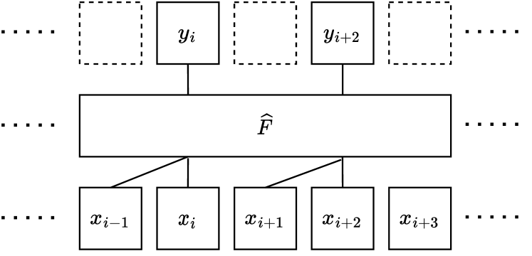
Figure 1: The self-attention mechanism can attend by relative position. In this diagram, each token attend to the previous token and itself.

Remark 4.3.

The results in Theorem 4.2 can be extended to the 2D input setting like image processing by modifying the positional encoding as $p_{ij}=[0,\dots,0,\cos(i\phi),\sin(i\phi),\cos(j\phi),\sin(j\phi)]$, where $i,j$ represent the row index and column index of the token $x_{ij}$, respectively. That is, Transformer can approximate both vertically and horizontally shift-equivariant functions with 2D inputs under appropriate assumptions. Similarly, the other results in this paper can be extended to the 2D input setting. Therefore, to some extent, our analysis explains the practical success of Transformers in the field of image processing (Dosovitskiy et al., 2021).

4.2 Piecewise Smoothness

Next, we derive the approximation error for the piecewise mixed and anisotropic smoothness, where the smoothness depends on each input. For the piecewise smoothness, we assume the following.

Assumption 4.4.

The true function $F^{\circ}$ is shift-equivariant and satisfies

$$F^{\circ}_{0} \in U(\mathcal{P}_{p,\theta}^{\gamma}),~{}\norm{F^{\circ}_{0}}_{\infty}\leq R,$$

where $R$ is a constant, $\gamma$ is mixed or anisotropic smoothness, and the smoothness parameters $a$ satisfies $a_{ij}=\Omega(j^{\alpha})$ and $\norm{a}_{wl^{\alpha}}\leq 1$ for some $0<\alpha<\infty$. For the mixed smoothness, we also assume $\bar{a}_{1}<\bar{a}_{2}$. In addition, we assume the importance function $\mu$ satisfies Assumption 4.1 with $p=\infty,R=1$.

For piecewise $\gamma$-smooth functions, it is necessary to extract important features depending on each input as shown in Fig. 2. Since $\Pi$ is not a linear operator, linear dimension reduction methods such as PCA and linear convolutional layers cannot approximate $\Pi$. However, due to the dynamical feature extraction ability of self-attention mechanism, Transformers can approximate $\Pi$ and achieve similar approximation error results as in the fixed smoothness setting.

Theorem 4.5.

For $d^{\prime}=O(T^{2(\beta+1)/\alpha}\log V)$, let $\{u_{i}\}_{i=1}^{2V+1}\subset\mathbb{R}^{d^{\prime}}$ be approximately orthonormal vectors which satisfies

$$\absolutevalue{\expectationvalue{u_{i},u_{j}}} \leq\varepsilon,~{}\expectationvalue{u_{i},u_{i}}=1.$$

In addition, We define $u_{i}$ for $i\notin[2V+1]$ by $u_{i}:=u_{i\mod(2V+1)}$. Suppose that the target function $F^{\circ}$ satisfies Assumption 4.4.

Then, for any $T>0$, there exists a transformer $\hat{F}\in\mathcal{T}(M,U,D,H,L,W,S,B)$ such that

$$\norm{\hat{F}_{i}-F^{\circ}_{i}}_{2,P_{X}}\lesssim 2^{-T}$$

for any $i\in\mathbb{Z}$, where

$$\begin{split}M&\sim T^{1/\alpha},~{}D\sim T^{2(\beta+1)/\alpha}\log V,\\ \log U_{1}&\sim\log T,~{}U_{i}=V~{}(i\geq 2),~{}H\sim(\log T)^{1/\alpha},\\ L&\sim\max\quantity{T^{2/\alpha},T^{2}},~{}W\sim T^{1/\alpha}2^{T/a^{\dagger}},\\ \log B&\sim\max\quantity{T^{1/\alpha},T,\log\log V}\\ S&\sim T^{2/\alpha}\max\quantity{T^{2/\alpha},T^{2}}2^{T/a^{\dagger}},\\ p_{i}&=[0,\dots,0,1,\cos(i\phi),\sin(i\phi),u_{i}^{\top}]^{\top}.\end{split}$$ (4)

See Appendix F for the proof. This theorem implies that multilayer Transformer networks can approximate mixed and anisotropic smooth functions even if inputs and outputs are infinite dimensional, and the smoothness structure depends on each input. In addition, the convergence rate is $N^{-a^{\dagger}}$, which is the same as in Theorem 4.2. This can be realized by the dynamical feature extraction ability of the self-attention mechanism. See Fig. 2 for an illustration of the feature extraction mechanism. The construction consists of two phases. First, the first layer of the Transformer network approximates the importance function $\mu$. Next, the Transformer network selects important tokens by the self-attention mechanism based on the estimated importance. Thanks to the softmax operation in the self-attention mechanism, Transformers can extract the most important token. However, it is difficult to extract the second (and subsequent) most important tokens. To overcome this issue, we developed a novel approximately orthonormal basis coding technique for the positional encoding to memorize already extracted tokens. Approximately orthonormal vectors can be constructed via random sampling, as shown in Lemma C.3.

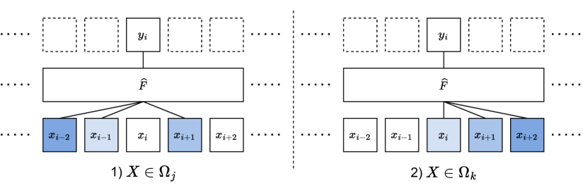
Figure 2: For piecewise $\gamma$-smoothness, the position of important tokens depends on each input. We show important tokens in darker color. In the case of $X\in\Omega_{j}$, the most important token to $y_{i}$ is $x_{i-2}$ and in the case of $X\in\Omega_{k}$, $x_{i+2}$ is the most important. The self-attention mechanism can switch its attention (represented by black lines) depending on the importance of tokens.

In this setting, the attention weights dynamically change depending on each input. This is in contrast to the existing works (Edelman et al., 2022; Okumoto & Suzuki, 2022), which studied the feature extraction ability of Transformer networks and CNNs, respectively. Our result matches the empirical findings (Likhosherstov et al., 2021) and Theorem 4.5 theoretically supports the dynamical feature extraction ability of the self-attention mechanism by considering the novel function class.

5 Estimation Error Analysis

In this section, we show that Transformer networks can achieve polynomial estimation error rate and avoid the curse of dimensionality.

To evaluate the variance of estimators, the covering number is often used to capture the complexity of model classes.

Definition 5.1 (Covering Number).

For a normed space $\mathcal{F}$ with a norm $\norm{\cdot}$, the $\delta$-covering number is defined as

$$\mathcal{N}(\mathcal{F},\delta,\norm{\cdot}) :=\inf\left\{n\in\mathbb{N}\mid\exists(f_{1},\dots,f_{n})\in\mathcal{F},\right.$$

$$\left.\forall f\in\mathcal{F},\exists i\in[n],\norm{f_{i}-f}\leq\delta\right\}.$$

For non-parametric regression problems with infite dimensional inputs and outputs, the estimation error of an ERM estimator is evaluated as follows.

Theorem 5.2.

For a given class $\mathcal{F}$ of functions from $[0,1]^{d\times\infty}$ to $\mathbb{R}^{\infty}$, let $\hat{F}\in\mathcal{F}$ be an ERM estimator which minimizes the empirical cost. Suppose that there exists a constant $R>0$ such that $\norm{F^{\circ}}_{\infty}\leq R$, $\norm{F}_{\infty}\leq R$ for any $F\in\mathcal{F}$, and $\mathcal{N}(\mathcal{F},\delta,\norm{\cdot}_{\infty})\geq 3$. Then, for any $0<\delta<1$, it holds that

$$R_{l,r}(\hat{F},F^{\circ})\leq 4\inf_{F\in\mathcal{F}}\frac{1}{r-l+1}\sum_{i=l}^{r}\norm{F_{i}-F^{\circ}_{i}}_{2,P_{X}}^{2}$$

$$\quad+C((R^{2}+\sigma^{2})\frac{\log\mathcal{N}(\mathcal{F},\delta,\norm{\cdot}_{\infty})}{n}+(R+\sigma)\delta),$$

where $C>0$ is a global constant.

This theorem is a direct extension of Lemma 4 in Schmidt-Hieber (2020) and Theorem 2.6 in Hayakawa & Suzuki (2020) to the multiple output setting. The proof can be found in Appendix G.

By carefully evaluating the complexity of the class of Transformer networks, we have the following bound on the log covering number of Transformer networks.

Theorem 5.3.

For given hyperparameters $M,U,D,H,L,W,S,B$, assume that $B\geq 1$ and $\norm{P}_{\infty}\leq B$. Then, we have the following log covering number bound:

$$\log\mathcal{N}(\mathcal{T}(M,U,D,H,L,W,S,B),\delta,\norm{\cdot}_{\infty})$$

$$\quad\lesssim M^{3}L(S+HD^{2})\log\quantity(\frac{DHLWB}{\delta}).$$

See Appendix H for the proof. Interestingly, the covering number bound does not depend on the dimensionality of inputs and outpus, and the width of the sliding window. This is because the number of parameters does not depend on these quantities due to the parameter sharing property and the magnitude of the hidden states are independent of the window size since the attention weights $A$ are normalized as $\norm{A}_{1}=1$. The parameter sharing property, on the other hand, leads to the limited interaction among tokens. This makes approximation analysis difficult, and thus it is necessary to design positional encoding carefully as mentioned in Section 4.

Combining above results, we have the following estimation error bound for the mixed and anisotropic smoothness.

Theorem 5.4.

Suppose that Assumption 4.1 holds. Let $\hat{F}$ be an ERM estimator in $\mathcal{T}_{R}(M,U,D,H,L,W,S,B)$, where $M,U,D,H,L,W,S,B$ is defined as (3) and $T=\frac{a^{\dagger}}{2a^{\dagger}+1}\log n$. Then, for any $l,r\in\mathbb{Z}$, we have

$$R_{l,r}(\hat{F},F) \lesssim n^{-\frac{2a^{\dagger}}{2a^{\dagger}+1}}(\log n)^{2/\alpha+2+\max\quantity{4/\alpha,4}}.$$

This can be shown by letting $\delta=1/n$ in Theorem 5.2. See Appendix I for the proof. The results show that the convergence rate of the estimation error does not depend on the input dimensionality and the output size if the smoothness of the target function has sparse structure. This implies that Transformers can avoid the curse of dimensionality. When $d=1$, this convergence rate matches that for CNNs (Okumoto & Suzuki, 2022) for single output setting. For anisotropic smoothness, this rate also matches, up to poly-log order, that of FNNs in the finite dimensional setting, which is known to be minimax optimal (Suzuki & Nitanda, 2021). That is, Transformers can achieve near-optimal rate in a minimax sense.

In addition, the Transformer architecture including the positional encoding $P$ does not depend directly on the smoothness structure $a$. This implies that Transformer networks can find important features and select them adaptively to the smoothness of the target function by learning the intrinsic structure of the target function.

For the piecewise smoothness, we have the following estimation error bound.

Theorem 5.5.

Suppose that Assumption 4.4 holds. Let $\hat{F}$ be an ERM estimator in $\mathcal{T}_{R}(M,U,D,H,L,W,S,B)$, where $M,U,D,H,L,W,S,B$ is defined as (4) and $T=\frac{a^{\dagger}}{2a^{\dagger}+1}\log n$. Then, for any $l,r\in\mathbb{Z}$, we have

$$R_{l,r}(\hat{F},F) \lesssim n^{-\frac{2a^{\dagger}}{2a^{\dagger}+1}}(\log n)^{5/\alpha+2+\max\quantity{4/\alpha,4}}(\log V)^{3}.$$

See Appendix J for the proof. This convergence rate is the same as in Theorem 5.4 up to poly-log order if $V=\operatorname{poly}(n)$. This means that Transformers can avoid the curse of dimensionality even if the smoothness architecture depends on each input.

In addition, the Transformer architecture does not depend on the partition $\quantity{\Omega_{\lambda}}_{\lambda\in\Lambda}$ and the importance function $\mu$. This means that Transformers can adapt to the intrinsic structure of the target function and realize the dynamical feature extraction according to the importance of tokens. This fact supports the practical success of Transformer networks in a wide range of applications with various structures.

6 Numerical Experiments

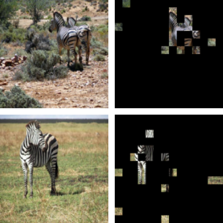
Figure 3: Two zebra images (left) and the corresponding images with 180 / 196 patches masked (right).

The assumptions in this paper essentially impose the sparsity of important features. To verify this, we conducted some numerical experiments using masked images as inputs. In this experiment, we prepared a pre-trained model (ViT-Base model (Dosovitskiy et al., 2021)) and two images of zebras in Fig. 3 from the validation set of ImageNet-1k (Russakovsky et al., 2015). We divided each image into $14\times 14$ tokens and masked each token in turn. At each step, a token to be masked is selected using a greedy algorithm to maximize the predicted probability of the correct class by the pre-trained model. Since masking informative features strongly affects the predicted probability, important features will remain unmasked near the end of the procedure.

As shown in Fig. 4, the predicted probability remains high and the model can classify the image correctly even if about 90% of the input is masked. This means that a small fragment of the image is important for prediction. In addition, Fig. 3 demonstrates that the patterns of unmasked, i.e., important features in the two images differ significantly. This implies important features change depending on each input and the piecewise smoothness describes more practical situations than the fixed smoothness.

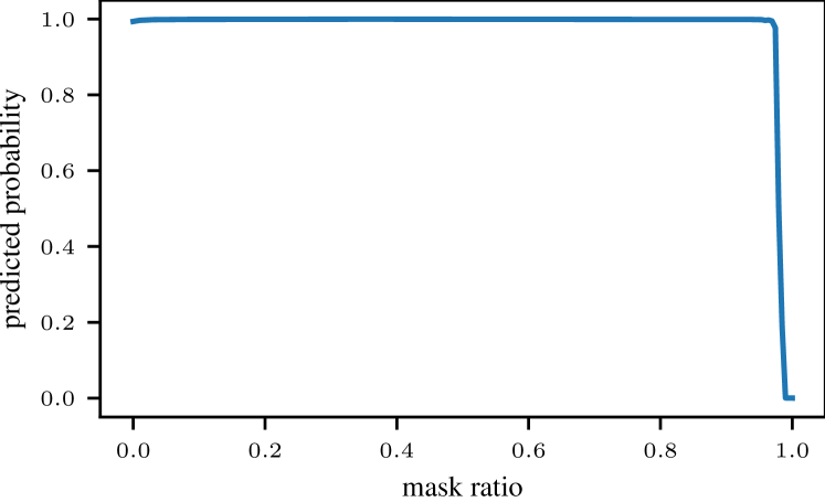
Figure 4: The predicted probability of the correct class for the top left image in Fig. 3. The predicted probability remains high even when most of the images are masked.

7 Conclusion

In this study, we have investigated the learnability of Transformer networks for sequence-to-sequence functions with infinite dimensional inputs. We have shown that Transformer networks can achieve a polynomial order convergence rate of estimation error when the smoothness of the target function has sparse structure. In addition, we have considered the situations where the smoothness depends on each input. Then, we have shown that Transformer networks can avoid the curse of dimensionality by switching the focus of attention based on input. We believe that our theoretical analysis provides a new insight into the nature of Transformer architecture.

Appendix A Notation List

Table 1: Notation list

Notation	Definition
$n$	sample size
$d$	token dimension
$(X^{(i)},y^{(i)})$	$i$-th observation
$\mathcal{D}^{n}=\quantity{(X^{(i)},y^{(i)})}_{i=1}^{n}$	training data
$P_{X}$	data distribution
$\Omega$	support of $P_{X}$
$\quantity{\Omega_{\lambda}}_{\lambda\in\Lambda}$	disjoint partition of $\Omega$
$\mathcal{F}_{p,\theta}^{\gamma}$	$\gamma$-smooth function class
$\mathcal{G}_{p,\theta}^{\gamma}$	piecewise $\gamma$-smooth function class
$\sigma$	noise variance
$F^{\circ}$	true function
$a$	smoothness parameter
$\bar{a}=[a_{i_{1},j_{1}},\dots,a_{i_{k},j_{k}},\dots]$	smoothness parameter sorted in the ascending order
$\tilde{a}$	$\quantity(\sum_{i=1}^{\infty}\bar{a}_{i}^{-1})^{-1}$
$a^{\dagger}$	$\bar{a}_{1}$ for the mixed smoothness and $\tilde{a}$ for the anisotropic smoothness
$\mu$	importance function
$\eta$	ReLU activation function
$I(T,\gamma)$	$\quantity{(i,j)\mid\exists s\in\mathbb{N}_{0}^{d\times\infty},s_{ij}\neq 0,\gamma(s)<T}$
$I_{j}(T,\gamma)$	$\quantity{i\mid(i,j)\in I(T,\gamma)}$
$e_{i}\in\mathbb{R}^{[l:r]}~{}(i\in[l:r])$	standard basis of $\mathbb{R}^{[l:r]}$
$\delta_{i,j}\in\mathbb{R}^{[l_{1}:r_{1}]\times[l_{2}:r_{2}]}~{}(i\in[l_{1},r_{1}],~{}j\in[l_{2}:r_{2}])$	$\delta_{i,j}:=e_{i}e_{j}^{\top}$
$x\overset{\epsilon}{\eqsim}y~{}(x,y\in\mathbb{R}^{d})$	$\norm{x-y}_{2}\lesssim\epsilon$
$1_{A}$	1 if $A$ is true and 0 if $A$ is false

Appendix B Extension to the Original Architecture

In this paper, we consider the multilayer FNN without skip connection while the FNN in the original architecture (Vaswani et al., 2017) uses single hidden layer with skip connection. However, our argument can be applied to the original structure with slight modifications as follows.

• (Skip connection) Since there exists an FNN $f:\mathbb{R}^{d}\to\mathbb{R}^{d}$ with one hidden layer of width $2d$ which works as an identity map, we can cancel out the skip connection using $f$. This modification does not change the order of hyperparameters, and we can obtain the same convergence rate as the original one.

• (One hidden layer) By letting $V_{h}=O$ in a self-attention layer, the self-attention layer behaves as an identity map due to the skip connection in the self-attention layer. Therefore, $L$-layer Transformer blocks (one block consists of an FNN layer with one hidden layer and a self-attention layer) can represent an $L$-layer FNN. Then, we can obtain the same convergence rate as the original one up to poly-log order.

Appendix C Auxiliary Lemmas

Lemma C.1.

For $\theta\in\mathbb{R}^{d}$, assume that there exist an index $i^{*}\in[d]$ and $\delta>0$ such that $\theta_{i^{*}}\geq\theta_{i}+\delta$ for any $i\neq i^{*}$. Then, we have

$$\norm{\operatorname{Softmax}(\theta)-e_{i^{*}}}_{1} \leq 2de^{-\delta}.$$

Proof.

For $i\neq i^{*}$, the assumption $\theta_{i^{*}}\geq\theta_{i}+\delta$ yields that

$$0 \leq\operatorname{Softmax}(\theta)_{i}=\frac{e^{\theta_{i}}}{\sum_{j=1}^{d}e^{\theta_{j}}}\leq e^{\theta_{i}-\theta_{i^{*}}}\leq e^{-\delta}.$$

For $i^{*}$, we have

$$0 \leq 1-\operatorname{Softmax}(\theta)_{i^{*}}=\sum_{i\neq i^{*}}\operatorname{Softmax}(\theta)_{i}\leq(d-1)e^{-\delta}.$$

Therefore,

$$\norm{\operatorname{Softmax}(\theta)-e_{i^{*}}}_{1} =\absolutevalue{1-\operatorname{Softmax}(\theta)_{i^{*}}}+\sum_{i\neq i^{*}}\absolutevalue{\operatorname{Softmax}(\theta)_{i}}\leq 2de^{-\delta},$$

which completes the proof. ∎

Lemma C.2.

For any $\theta,\theta^{\prime}\in\mathbb{R}^{d}$, we have

$$\norm{\operatorname{Softmax}(\theta)-\operatorname{Softmax}(\theta^{\prime})}_{1} \leq 2\norm{\theta-\theta^{\prime}}_{\infty}.$$

Proof.

See Corollary A.7 in Edelman et al. (2022). ∎

Lemma C.3.

For any $l\in\mathbb{N}$ and $\varepsilon>0$, there exists $\varepsilon$-approximately orthonormal vectors $\quantity{u_{i}}_{i=1}^{l}\subset\mathbb{R}^{d}~{}(d=O\quantity(\frac{\log l}{\varepsilon^{2}}))$ which satisfies

$$\begin{split}\absolutevalue{\expectationvalue{u_{i},u_{j}}}&\leq\varepsilon,\\ \expectationvalue{u_{i},u_{i}}&=1,\end{split}$$ (5)

for any $i\neq j$.

Proof.

Let each component of $u_{i}\in\mathbb{R}^{d}$ independently follows Bernoulli distribution $\Pr((u_{i})_{j}=\pm 1/\sqrt{d})=1/2$. Then, we have $\norm{u_{i}}=1$. Since $\expectationvalue{u_{i},u_{j}}$ can be seen as the sum of independent Bernoulli random variables, a Chernoff bound implies

$$\Pr(\absolutevalue{\expectationvalue{u_{i},u_{j}}}>\varepsilon) \leq 2\exp(-\frac{\varepsilon^{2}}{2}d).$$

By letting $d=\frac{4\log 2l}{\varepsilon^{2}}$, we have

$$\Pr(\absolutevalue{\expectationvalue{u_{i},u_{j}}}>\varepsilon) \leq 2\exp(-2\log 2l)=\frac{1}{2l^{2}}.$$

Since there exists at most $l^{2}/2$ pairs $(i,j)$, from the union bound, the probability that $\absolutevalue{\expectationvalue{u_{i},u_{j}}}\leq\varepsilon$ for all $(i,j)$ such that $i\neq j$ is greater than $1-\frac{l^{2}}{2}\cdot\frac{1}{2l^{2}}=3/4$. This means there exist approximately orthonormal vectors which satisfy Eq. (5). ∎

Lemma C.4.

For $B\geq 1$, let $f\in\Psi(L,W,B,S)$, and $g\in\mathcal{A}(U,D,H,B)$. Then, for any $r\geq 1$, $x,x^{\prime}\in\mathbb{R}^{d}$ and $X,X^{\prime}\in[-r,r]^{d\times\infty}$, we have

$$\norm{f(x)-f(x^{\prime})}_{\infty} \leq(BW)^{L}\norm{x-x^{\prime}}_{\infty}\leq(6HDBW)^{4L}r^{2}\norm{x-x^{\prime}}_{\infty},$$ (6)

$$\norm{g(X)-g(X^{\prime})}_{\infty} \leq 6HB^{3}D^{4}r^{2}\norm{X-X^{\prime}}_{\infty}\leq(6HDBW)^{4L}r^{2}\norm{X-X^{\prime}}_{\infty}.$$

Proof.

Since the ReLU activation function $\eta$ is $1$-Lipschitz continuous and $\norm{W_{i}x+b-(W_{i}x^{\prime}+b)}_{\infty}\leq BW\norm{x-x^{\prime}}_{\infty}$, $f$ is $(BW)^{L}$-Lipschitz continuous. This implies Eq. (6).

Let $\bar{X}:=X[-U:U]$ and $A_{h}:=\operatorname{Softmax}((K_{h}\bar{X})^{\top}(Q_{h}x_{i}))$. We define $\bar{X}^{\prime},A^{\prime}_{h}$ in the same way as $\bar{X},A_{h}$. Then, we have

$$\norm{g(X)_{i}-g(X^{\prime})_{i}}_{\infty} \leq\norm{x_{i}-x^{\prime}_{i}}_{\infty}+\sum_{h=1}^{H}\norm{V_{h}\bar{X}A_{h}-V\bar{X}^{\prime}A^{\prime}_{h}}_{\infty}$$

$$\leq\norm{x_{i}-x^{\prime}_{i}}_{\infty}+\sum_{h=1}^{H}\norm{V_{h}\bar{X}A_{h}-V\bar{X}A^{\prime}_{h}}_{\infty}+\norm{V\bar{X}A^{\prime}_{h}-V\bar{X}^{\prime}A^{\prime}_{h}}_{\infty}.$$

From Lemma C.2, we have

$$\norm{A_{h}-A_{h}^{\prime}}_{1} \leq 2\norm{(K_{h}\bar{X})^{\top}(Q_{h}x_{i})-(K\bar{X}^{\prime})^{\top}(Q_{h}x^{\prime}_{i})}_{\infty}$$

$$\leq 2\norm{(K_{h}\bar{X})^{\top}(Q_{h}x_{i})-(K\bar{X})^{\top}(Q_{h}x^{\prime}_{i})}_{\infty}+2\norm{(K_{h}\bar{X})^{\top}(Q_{h}x^{\prime}_{i})-(K_{h}\bar{X}^{\prime})^{\top}(Q_{h}x^{\prime}_{i})}_{\infty}$$

$$\leq 4rB^{2}D^{3}\norm{X_{i}-X^{\prime}_{i}}_{\infty}.$$

Here, we used the fact that $\norm{K_{h}}_{\infty},\norm{Q_{h}}_{\infty},\norm{V_{h}}_{\infty}\leq B$ and $\norm{X}_{\infty}\leq r$. Then, it holds that

$$\norm{V_{h}\bar{X}A_{h}-V_{h}\bar{X}A^{\prime}_{h}}_{\infty} \leq BDr\norm{A_{h}-A^{\prime}_{h}}_{1}$$

$$\leq 4B^{3}D^{4}r^{2}\norm{X_{i}-X^{\prime}_{i}}_{\infty},$$

$$\norm{V_{h}\bar{X}A^{\prime}_{h}-V_{h}\bar{X}^{\prime}A^{\prime}_{h}}_{\infty} \leq BD\norm{X-X^{\prime}}_{\infty}.$$

Since $B\geq 1,r\geq 1$, we have

$$\norm{g(X)_{i}-g(X^{\prime})_{i}}_{\infty} \leq\quantity(1+4B^{3}D^{4}r^{2}+BD)\norm{X-X^{\prime}}_{\infty}$$

$$\leq 6HB^{3}D^{4}r^{2}\norm{X-X^{\prime}}_{\infty},$$

which completes the proof. ∎

Lemma C.5.

Let $f\in\Psi(L,W,S,B)$ and $g\in\mathcal{A}(U,D,H,B)$ for $B\geq 1$. For any $r\geq 1$, $X~{}(\norm{X}_{\infty}\leq r)$, and $x~{}(\norm{x}_{\infty}\leq r)$, we have

$$\norm{f(x)}_{\infty} \leq(2BW)^{L}r\leq(6HDBW)^{L}r,$$

$$\norm{g(X)}_{\infty} \leq 2HBDr\leq(6HDBW)^{L}r.$$

Proof.

For the FNN layer $f$, since $\norm{\eta(z)}_{\infty}\leq\norm{z}_{\infty}$ and

$$\norm{Wz+b}_{\infty} \leq BWr^{\prime}+B$$

$$\leq 2BWr^{\prime}$$

for $\norm{z}_{\infty}\leq r^{\prime}~{}(r^{\prime}\geq 1)$, we have

$$\norm{f(X)}_{\infty} \leq(2BW)^{L}r$$

by induction.

For attention layer $g$, define $\bar{X}$ and $A_{h}$ as in the proof of Lemma C.4. Then, we have

$$\norm{g_{i}(X)}_{\infty} \leq\norm{x_{i}}_{\infty}+\sum_{i=1}^{H}\norm{V\bar{X}A_{h}}_{\infty}$$

$$\leq\norm{X}_{\infty}+HBD\norm{X}_{\infty}\norm{A_{h}}_{1}$$

$$\leq 2HBDr,$$

since $\norm{A_{h}}_{1}=1$. This completes the proof. ∎

Lemma C.6.

Define $f,\tilde{f}\in\Psi(L,W,B,S)$ by

$$f(x) :=(A_{L}\cdot+b_{L})\circ\dots\circ(A_{1}x+b_{1})$$

$$\tilde{f}(x) :=(\tilde{A}_{L}\cdot+\tilde{b}_{L})\circ\dots\circ(\tilde{A}_{1}x+\tilde{b}_{1}),$$

where $\norm{A_{i}-\tilde{A}_{i}}_{\infty}\leq\delta,\norm{b_{i}-\tilde{b}_{i}}_{\infty}\leq\delta$ for a given $\delta>0$. For any $r\geq 1$ and $x~{}(\norm{x}_{\infty}\leq r)$, we have

$$\norm{f(x)-\tilde{f}(x)}_{\infty} \leq 2(2BW)^{L}\delta r\leq(6HDBW)^{4L}\delta r^{3}.$$

In addition, define $g,\hat{g}\in\mathcal{A}(U,D,H,B,S)$ by

$$g(X)_{i} :=x_{i}+\sum_{i=1}^{H}V_{h}X[-U:U]\operatorname{Softmax}((K_{h}X[-U:U])^{\top}(Q_{h}x_{i}))$$

$$\tilde{g}(X)_{i} :=x_{i}+\sum_{i=1}^{H}\tilde{V}_{h}X[-U:U]\operatorname{Softmax}((\tilde{K}_{h}X[-U:U])^{\top}(\tilde{Q}_{h}x_{i})),$$

where $\norm{K_{h}-\tilde{K}_{h}}_{\infty}\leq\delta$, $\norm{Q_{h}-\tilde{Q}_{h}}_{\infty}\leq\delta$, and $\norm{V_{h}-\tilde{V}_{h}}_{\infty}\leq\delta$ for a given $\delta>0$. For any $r\geq 1$ and $X~{}(\norm{X}_{\infty}\leq r)$, we have

$$\norm{g(X)-\tilde{g}(X)}_{\infty} \leq 5HB^{2}D^{4}r^{3}\delta\leq(6HDBW)^{4L}\delta r^{3}.$$

Proof.

By the same argument as Lemma 3 in Suzuki (2018), we have

$$\norm{f(x)-\tilde{f}(x)}_{\infty} \leq 2(2BW)^{L}r\delta.$$

Define $\bar{X},A_{h},\tilde{A}_{h}$ as in Lemma C.4. From Lemma C.2, we have

$$\norm{A_{h}-\tilde{A}_{h}}_{1} \leq 2\norm{(K_{h}\bar{X})^{\top}(Q_{h}x_{i})-(\tilde{K}_{h}\bar{X})^{\top}(\tilde{Q}_{h}x_{i})}_{\infty}$$

$$\leq 2\norm{(K_{h}\bar{X})^{\top}(Q_{h}x_{i})-(K_{h}\bar{X})^{\top}(\tilde{Q}_{h}x_{i})}_{\infty}+2\norm{(K_{h}\bar{X})^{\top}(\tilde{Q}_{h}x_{i})-(\tilde{K}_{h}\bar{X})^{\top}(\tilde{Q}_{h}x_{i})}_{\infty}$$

$$\leq 4(BD^{3}r^{2}\delta).$$

Therefore, it holds that

$$\norm{g(X)_{i}-\tilde{g}(X)_{i}}_{\infty} \leq\sum_{i=1}^{H}\norm{V_{h}\bar{X}A_{h}-\tilde{V}_{h}\bar{X}\tilde{A}_{h}}_{\infty}$$

$$\leq\sum_{i=1}^{H}\norm{V_{h}\bar{X}(A_{h}-\tilde{A}_{h})}_{\infty}+\norm{(V_{h}-\tilde{V}_{h})\bar{X}\tilde{A}_{h}}_{\infty}$$

$$\leq\sum_{i=1}^{H}\norm{V_{h}\bar{X}}_{\infty}\norm{A_{h}-\tilde{A}_{h}}_{1}+\norm{(V_{h}-\tilde{V}_{h})\bar{X}}_{\infty}$$

$$\leq H(4(B^{2}D^{4}r^{3}\delta)+D\delta r)$$

$$\leq 5HB^{2}D^{4}r^{3}\delta,$$

which completes the proof. ∎

Lemma C.7.

Assume that positive and monotonically non-decreasing sequences $\bar{a}=\quantity{\bar{a}_{i}}_{i=1}^{\infty}$ and $\bar{a}^{\prime}=\quantity{\bar{a}^{\prime}_{i}}_{i=1}^{\infty}$ satisfies $\bar{a}_{1}\geq 1=\bar{a}^{\prime}_{1}$ and

$$\prod_{i=2}^{\infty}\frac{1}{1-2^{-(\bar{a}_{i}-\bar{a}_{1})}} <\infty,$$

$$\prod_{i=2}^{\infty}\frac{1}{1-2^{-\beta(\bar{a}_{i}-\bar{a}^{\prime}_{i})}} <\infty,$$

for a positive constant $\beta$. Then, we have

$$\sum_{s\in\mathbb{N}_{0}^{\infty}:\expectationvalue{\bar{a}^{\prime},s}\geq T}2^{-\beta\expectationvalue{\bar{a},s}} \leq(1-2^{-\beta})^{-1}\quantity(\prod_{i=2}^{\infty}\frac{1}{1-2^{-\beta(\bar{a}_{i}-\bar{a}^{\prime}_{i})}})2^{-\beta T},$$

$$\sum_{s\in\mathbb{N}_{0}^{\infty}:\expectationvalue{\bar{a},s}<T}2^{s} \leq 8\quantity(\prod_{i=2}^{\infty}\frac{1}{1-2^{-(\bar{a}_{i}-\bar{a}_{1})}})2^{T}.$$

Proof.

See Lemma 18 in Okumoto & Suzuki (2022). ∎

Appendix D Approximation ability of FNN

In this section, we show that an FNN can approximate (piecewise) $\gamma$-smooth function if important features are extracted properly. For a general $\gamma$-smooth function class, we have the following approximation error bound.

Lemma D.1.

For $\gamma:\mathbb{N}_{0}^{d\times\infty}\to\mathbb{R}_{>0}$, let

$$G(T,\gamma) :=\sum_{s\in\mathbb{N}_{0}^{d\times\infty}:\gamma(s)<T}2^{s},$$

$$f_{\max}(T,\gamma) :=\max_{s\in\mathbb{N}_{0}^{d\times\infty}:\gamma(s)<T}\max_{i\in[d],j\in\mathbb{Z}}s_{ij},$$

$$I(T,\gamma) :=\quantity{(i,j)\mid\exists s\in\mathbb{N}_{0}^{d\times\infty},s_{ij}\neq 0,\gamma(s)<T},$$

$$d_{\max}(T,\gamma) :=\absolutevalue{I(T,\gamma)}.$$

Assume that $\gamma^{\prime}$ satisfies $\gamma^{\prime}(s)<\gamma(s)$ and the target function $f\in\mathcal{F}_{p,\theta}^{\gamma}([0,1]^{d\times\infty})(p\geq 2,\theta\geq 1)$ satisfies $\norm{f}_{\infty}\leq R$ for a constant $R>0$.

For given $T>0$, let

$$(d_{\max},f_{\max},G) :=\begin{cases}(d_{\max}(T,\gamma),f_{\max}(T,\gamma),G(T,\gamma)),&\quad(\theta=1),\\ (d_{\max}(T,\gamma^{\prime}),f_{\max}(T,\gamma^{\prime}),G(T,\gamma^{\prime})),&\quad(\theta>1),\end{cases}$$

and

$$\begin{split}L&:=2K\max\quantity{d_{\max}^{2},T^{2},(\log G)^{2},\log f_{\max}},\\ W&:=21d_{\max}G,\\ S&:=1764Kd_{\max}^{2}\max\quantity{d_{\max}^{2},T^{2},(\log G)^{2},\log f_{\max}}G,\\ B&:=2^{d_{\max}/2}K^{\prime},\end{split}$$ (7)

for positive constants $K,K^{\prime}$ which depend on only $R$. Then, there exists an FNN $\hat{f}_{T}\in\Psi(L,W,B,S)$ such that

$$\norm{f-\hat{f}_{T}\circ\Gamma}_{2,P_{X}} \lesssim\begin{cases}2^{-T}\norm{f}_{\mathcal{F}_{p,\theta}^{\gamma}},&\quad(\theta=1),\\ \quantity(\sum_{T\leq\gamma(s)}2^{\frac{\theta}{\theta-1}(\gamma^{\prime}(s)-\gamma(s))})^{1-1/\theta}2^{-T}\norm{f}_{\mathcal{F}_{p,\theta}^{\gamma}},&\quad(\theta>1),\end{cases}$$

where $\Gamma:\mathbb{R}^{d\times\infty}\to\mathbb{R}^{d_{\max}}$ is a feature extractor defined by

$$\begin{split}\Gamma(X):=[X_{i_{1},j_{1}},\dots,X_{i_{d_{\max}},j_{d_{\max}}}]\end{split}$$ (8)

for $X\in\mathbb{R}^{d\times\infty}$, and $I(T,\gamma)=\quantity{(i_{1},j_{1}),\dots,(i_{d_{\max}},j_{d_{\max}})}$.

Proof.

Define $f_{T}$ by $f_{T}=\sum_{\gamma(s)<T}\delta_{s}(f)$ for $\theta=1$ and $f_{T}=\sum_{\gamma^{\prime}(s)<T}\delta_{s}(f)$ for $\theta>1$. Then, for a given $\hat{f}\in\Psi(L,W,S,B)$, we have

$$\norm{f-\hat{f}\circ\Gamma}_{2,P_{X}} \leq\norm{f-f_{T}}_{2,P_{X}}+\norm{f_{T}-\hat{f}\circ\Gamma}_{2,P_{X}}.$$

First, we evaluate $\norm{f-f_{T}}_{2,P_{X}}$. By the Cauchy-Schwartz inequality, we have, for $p>2$,

$$\norm{\delta_{s}}_{2,P_{X}}^{2} =\int\absolutevalue{\delta_{s}(f)}^{2}\differential{P_{X}}$$

$$\leq\quantity(\int\quantity(\absolutevalue{\delta_{s}(f)}^{2})^{p/2}\differential{P_{X}})^{2/p}\quantity(\int 1\differential{P_{X}})^{1-2/p}$$

$$=\norm{\delta_{s}(f)}_{p,P_{X}}^{2}.$$

Therefore, for any $p\geq 2$, it holds that

$$\norm{\delta_{s}(f)}_{2,P_{X}} \leq\norm{\delta_{s}(f)}_{p,P_{X}}.$$

In the case of $\theta=1$, we have

$$\norm{f-f_{T}}_{2,P_{X}} =\norm{\sum_{\gamma(s)\geq T}\delta_{s}(f)}_{2,P_{X}}$$

$$\leq\sum_{\gamma(s)\geq T}\norm{\delta_{s}(f)}_{2,P_{X}}$$

$$\leq\sum_{\gamma(s)\geq T}\norm{\delta_{s}(f)}_{p,P_{X}}$$

$$=\sum_{\gamma(s)\geq T}2^{\gamma(s)}2^{-\gamma(s)}\norm{\delta_{s}(f)}_{p,P_{X}}$$

$$\leq 2^{-T}\sum_{\gamma(s)\geq T}2^{\gamma(s)}\norm{\delta_{s}(f)}_{p,P_{X}}$$

$$\leq 2^{-T}\norm{f}_{\mathcal{F}_{p,\theta}^{\gamma}}.$$

In the case of $\theta>1$, we have

$$\norm{f-f_{T}}_{2,P_{X}} \leq\sum_{\gamma^{\prime}(s)\geq T}\norm{\delta_{s}(f)}_{p,P_{X}}$$

$$=\sum_{\gamma^{\prime}(s)\geq T}2^{-\gamma^{\prime}(s)}2^{\gamma^{\prime}(s)-\gamma(s)}2^{\gamma(s)}\norm{\delta_{s}(f)}_{p,P_{X}}$$

$$\leq 2^{-T}\sum_{\gamma^{\prime}(s)\geq T}2^{\gamma^{\prime}(s)-\gamma(s)}2^{\gamma(s)}\norm{\delta_{s}(f)}_{p,P_{X}}$$

$$\leq 2^{-T}\quantity(\sum_{\gamma^{\prime}(s)\geq T}2^{\frac{\theta}{\theta-1}(\gamma^{\prime}(s)-\gamma(s))})^{1-1/\theta}\quantity(\sum_{\gamma^{\prime}(s)\geq T}2^{\theta\gamma(s)}\norm{\delta_{s}(f)}_{p,P_{X}}^{\theta})^{1/\theta}$$

$$\leq 2^{-T}\quantity(\sum_{\gamma^{\prime}(s)\geq T}2^{\frac{\theta}{\theta-1}(\gamma^{\prime}(s)-\gamma(s))})^{1-1/\theta}\norm{f}_{\mathcal{F}_{p,\theta}^{\gamma}}.$$

For the third inequality, we used Hölder inequality. Combining these two cases, we obtain

$$\norm{f-f_{T}}_{2,P_{X}} \leq\begin{cases}2^{-T}\norm{f}_{p,\theta}^{\gamma}&\quad(\theta=1),\\ \quantity(\sum_{\gamma^{\prime}(s)\geq T}2^{\frac{\theta}{\theta-1}(\gamma^{\prime}(s)-\gamma(s))})^{1-1/\theta}2^{-T}\norm{f}_{p,\theta}^{\gamma}&\quad(\theta>1).\end{cases}$$ (9)

From Lemma 17 in (Okumoto & Suzuki, 2022), there exists an FNN $\hat{f}_{T}\in\Psi(L,W,S,B)$ such that

$$\norm{f_{T}-\hat{f}_{T}\circ\Gamma}_{\infty} \leq 2^{-T}.$$ (10)

Combining Eq. (9) and (10), we have

$$\norm{f-\hat{f}_{T}\circ\Gamma}_{2,P_{X}} \lesssim\begin{cases}2^{-T}\norm{f}_{p,\theta}^{\gamma}&\quad(\theta=1),\\ \quantity(\sum_{\gamma^{\prime}(s)\geq T}2^{\frac{\theta}{\theta-1}(\gamma^{\prime}(s)-\gamma(s))})^{1-1/\theta}2^{-T}\norm{f}_{p,\theta}^{\gamma}&\quad(\theta>1).\end{cases}$$

This completes the proof. ∎

In addition, for a general piecewise $\gamma$-smooth function class, we have the following approximation error bound.

Lemma D.2.

For $\gamma:\mathbb{N}_{0}^{d\times(2V+1)}\to\mathbb{R}_{>0}$, let

$$G(T,\gamma) :=\sum_{s\in\mathbb{N}_{0}^{d\times(2V+1)}:\gamma(s)<T}2^{s},$$

$$f_{\max}(T,\gamma) :=\max_{s\in\mathbb{N}_{0}^{d\times(2V+1)}:\gamma(s)<T}\max_{i\in[d],j\in[2V+1]}s_{ij},$$

$$I(T,\gamma) :=\quantity{(i,j)\mid s\in\mathbb{N}_{0}^{d\times(2V+1)},s_{ij}\neq 0,\gamma(s)<T},$$

$$d_{\max}(T,\gamma) :=\absolutevalue{I(T,\gamma)}.$$

Assume that $\gamma^{\prime}$ satisfies $\gamma^{\prime}(s)<\gamma(s)$ and the target function $f\in\mathcal{P}_{p,\theta}^{\gamma}(p\geq 2,\theta\geq 1)$ satisfies $\norm{f}_{\infty}\leq R$ for a constant $R>0$.

For given $T>0$, let

$$(d_{\max},f_{\max},G) :=\begin{cases}(d_{\max}(T,\gamma),f_{\max}(T,\gamma),G(T,\gamma)),&\quad(\theta=1),\\ (d_{\max}(T,\gamma^{\prime}),f_{\max}(T,\gamma^{\prime}),G(T,\gamma^{\prime})),&\quad(\theta>1),\end{cases}$$

and define $L,W,S,B$ by Eq. (7). Then, there exists an FNN $\hat{f}_{T}\in\Psi(L,W,B,S)$ such that

$$\norm{f-\hat{f}_{T}\circ\Gamma\circ\Pi}_{2,P_{X}} \lesssim\begin{cases}2^{-T}\norm{f}_{\mathcal{P}_{p,\theta}^{\gamma}},&\quad(\theta=1),\\ \quantity(\sum_{T\leq\gamma(s)}2^{\frac{\theta}{\theta-1}(\gamma^{\prime}(s)-\gamma(s))})^{1-1/\theta}2^{-T}\norm{f}_{\mathcal{P}_{p,\theta}^{\gamma}},&\quad(\theta>1),\end{cases}$$

where $\Gamma:\mathbb{R}^{d\times(2V+1)}\to\mathbb{R}^{d_{\max}}$ is a feature extractor defined by

$$\begin{split}\Gamma(X):=[X_{i_{1},j_{1}},\dots,X_{i_{d_{\max}},j_{d_{\max}}}]\end{split}$$ (11)

for $X\in\mathbb{R}^{d\times(2V+1)}$, and $I(T,\gamma)=\quantity{(i_{1},j_{1}),\dots,(i_{d_{\max}},j_{d_{\max}})}$.

Proof.

From the definition of $\mathcal{P}_{p,\theta}^{\gamma}$, there exist $f^{\prime}\in\mathcal{F}_{p,\theta}^{\gamma}([0,1]^{d\times[2V+1]})$ such that $f=f^{\prime}\circ\Pi$. Define $f_{T}$ by $f_{T}:=\sum_{\gamma(s)<T}\delta_{s}(f^{\prime})$ for $\theta=1$ and $f_{T}:=\sum_{\gamma^{\prime}(s)<T}\delta_{s}(f^{\prime})$ for $\theta>1$. By the same argument as in the case of $\gamma$-smoothness, we have

$$\norm{f-f_{T}\circ\Pi}_{2,P_{X}} \leq 2^{-T}\norm{f}_{\mathcal{P}_{p,\theta}^{\gamma}}$$

for $\theta=1$, and

$$\norm{f-f_{T}\circ\Pi}_{2,P_{X}} \leq 2^{-T}\quantity(\sum_{\gamma^{\prime}(s)\geq T}2^{\frac{\theta}{\theta-1}(\gamma^{\prime}(s)-\gamma(s))})^{1-1/\theta}\norm{f}_{\mathcal{P}_{p,\theta}^{\gamma}}$$

for $\theta>1$. By the same argument as in Lemma 17 in (Okumoto & Suzuki, 2022), there exists an FNN $\hat{f}_{T}\in\Psi(L,W,S,B)$ such that

$$\norm{f_{T}-\hat{f}_{T}\circ\Gamma}_{\infty} \leq 2^{-T}.$$

This implies

$$\norm{f_{T}\circ\Pi-\hat{f}_{T}\circ\Gamma\circ\Pi}_{\infty} \leq 2^{-T}.$$

Therefore, we have

$$\norm{f-\hat{f}_{T}\circ\Gamma\circ\Pi}_{2,P_{X}} \leq\norm{f-f_{T}\circ\Pi}_{2,P_{X}}+\norm{f_{T}\circ\Pi-\hat{f}_{T}\circ\Gamma\circ\Pi}_{\infty}$$

$$\lesssim\begin{cases}2^{-T}\norm{f}_{\mathcal{P}_{p,\theta}^{\gamma}},&\quad(\theta=1),\\ \quantity(\sum_{T\leq\gamma(s)}2^{\frac{\theta}{\theta-1}(\gamma^{\prime}(s)-\gamma(s))})^{1-1/\theta}2^{-T}\norm{f}_{\mathcal{P}_{p,\theta}^{\gamma}},&\quad(\theta>1),\end{cases}$$

which completes the proof. ∎

Next, we evaluate the approximation ability of FNN for the (piecewise) mixed and anisotropic smoothness when the smoothness parameter $a$ satisfies $\norm{a}_{wl^{\alpha}}\leq 1$.

Theorem D.3.

Suppose that the target functions $f\in\mathcal{F}_{p,\theta}^{\gamma}$ and $g\in\mathcal{P}_{p,\theta}^{\gamma}$ satisfy $\norm{f}_{\infty}\leq R$ and $\norm{g}_{\infty}\leq R$, where $R>0$ and $\gamma$ is the mixed or anisotropic smoothness and the smoothness parameter $a$ satisfies $\norm{a}_{wl^{\alpha}}\leq 1$. For any $T>0$, there exist FNNs $\hat{f}_{T},\hat{g}_{T}\in\Psi(L,W,S,B)$ such that

$$\norm{\hat{f}_{T}\circ\Gamma-f}_{2,P_{X}} \lesssim 2^{-T},$$

$$\norm{\hat{g}_{T}\circ\Gamma\circ\Pi-g}_{2,P_{X}} \lesssim 2^{-T},$$

where

$$L \sim\max\quantity{T^{2/\alpha},T^{2}},W\sim T^{1/\alpha}2^{T/a^{\dagger}},$$

$$S \sim T^{2/\alpha}\max\quantity{T^{2/\alpha},T^{2}}2^{T/a^{\dagger}},\log B\sim T^{1/\alpha}.$$

The result for the fixed smoothness case is similar to Theorem 7 in Okumoto & Suzuki (2022), but we omit the case $1\leq p\leq 2$ since we relax the assumption $\norm{\frac{\differential{P_{X}}}{\differential{\lambda}}}_{\infty}<\infty$, which is imposed in the previous work.

Proof.

We show the result for the mixed smoothness and anisotropic smoothness separately.

Mixed smoothness

Let us consider the case $\theta=1$. Since $\norm{a}_{wl^{\alpha}}\leq 1$, $\bar{a}_{j}\geq j^{\alpha}$ for any $j\in\mathbb{N}$. Therefore, we see that $d_{\max}\sim T^{1/\alpha}$ and $f_{\max}\sim T$. In addition, from Lemma C.7, we have

$$G(T,\gamma) =\sum_{\expectationvalue{a/\bar{a}_{1},s}<T/\bar{a}_{1}}2^{s}\lesssim 2^{T/{\bar{a}_{1}}}.$$

Therefore, from Lemmas D.1 and D.2, there exists $\hat{f}_{T},\hat{g}_{T}\in\Psi(L,W,S,B)$ such that

$$\norm{\hat{f}_{T}\circ\Gamma-f}_{2,P_{X}} \lesssim 2^{-T},$$

$$\norm{\hat{g}_{T}\circ\Gamma\circ\Pi-g}_{2,P_{X}} \lesssim 2^{-T},$$

where $L,W,S,B$ is defined in Eq. (7).

In the case of $\theta>1$, let $\bar{a}^{\prime}_{1}=a_{1}/2$ and $\bar{a}^{\prime}_{i}=\bar{a}_{i}/u~{}(i\geq 2)$ for $2<u<2+\frac{2\delta}{\bar{a}_{1}}$, where $\delta=\bar{a}_{1}-\bar{a}_{2}>0$. Then, $\bar{a}^{\prime}$ is a positive monotonically increasing sequence. Since $\bar{a}_{i}\geq i^{\alpha}$, we have, for any $c>0$,

$$\prod_{i=2}^{\infty}\frac{1}{1-2^{-c\quantity(\bar{a}_{i}/\bar{a}_{1}-2\bar{a}^{\prime}_{i}/\bar{a}_{1})}} <\infty.$$

Therefore, by adjusting the scale of $\bar{a},\bar{a}^{\prime}$, Lemma C.7 yields that

$$\sum_{\expectationvalue{a^{\prime},s}\geq T}2^{\frac{\theta}{\theta-1}(\gamma^{\prime}(s)-\gamma(s))} \lesssim 2^{-\frac{\theta}{\theta-1}T},$$

$$G(T,\gamma^{\prime}) \lesssim 2^{T/\bar{a}^{\prime}_{1}}=2^{2T/\bar{a}_{1}}.$$

Therefore, from Lemma D.1, there exists $\hat{f}_{T},\hat{g}_{T}\in\Psi(L,W,S,B)$ such that

$$\norm{\hat{f}_{T}\circ\Gamma-f}_{2,P_{X}} \lesssim\quantity(2^{-\frac{\theta}{\theta-1}T})^{1-1/\theta}2^{-T}=2^{-2T},$$

$$\norm{\hat{g}_{T}\circ\Gamma\circ\Pi-g}_{2,P_{X}} \lesssim\quantity(2^{-\frac{\theta}{\theta-1}T})^{1-1/\theta}2^{-T}=2^{-2T}.$$

By replacing $2T\leftarrow T$, we obtain the result.

Anisotropic smoothness

For $s\in\mathbb{N}_{0}^{\infty}$, define $\bar{s}$ as the sequence rearranged in the same way as $\bar{a}$. Since $\gamma(s)\leq T$ is equivalent to $\bar{s}_{i}\leq T/\bar{a}_{i}$ for any $i\in\mathbb{N}$, we have

$$\sum_{\gamma(s)<T}2^{s}\leq\prod_{i=1}^{\infty}\quantity(\sum_{\bar{s}_{i}=0}^{\lceil T/\bar{a}_{i}\rceil}2^{\bar{s}_{i}}) \leq 2^{\sum_{i=1}^{\infty}\lceil T/\bar{a}_{i}\rceil}\sim 2^{T/\tilde{a}}.$$

Then, by the same argument as in the case of mixed smoothness, we obtain the result. ∎

Appendix E Proof of Theorem 4.2

First, we construct the embedding layer $\operatorname{Enc}_{P}$. Let $D$ be $d+d_{\max}+2$ and the embedding matrix $E\in\mathbb{R}^{D\times d}$ be the matrix such that $Ex=[x_{1},\dots,x_{d},0,\dots,0]^{\top}\in\mathbb{R}^{D}$ for any $x\in\mathbb{R}^{d}$. Note that $\norm{E}_{\infty}=1$. Define $Z^{(m)}$ by

$$\begin{split}Z^{(0)}&=\quantity{z^{(0)}_{j}}_{j=-\infty}^{\infty}:=\operatorname{Enc}_{P}(X),\\ Z^{(m)}&=\quantity{z^{(m)}_{j}}_{j=-\infty}^{\infty}:=g_{m}\circ f_{m-1}\circ g_{m-1}\circ\dots f_{1}\circ g_{1}\circ\operatorname{Enc}_{P}(X)\quad(j=1,\dots,M).\end{split}$$ (12)

Then, the embedded token $z^{(0)}_{j}$ is given by $[X_{1,j},\dots,X_{d,j},0,\dots,0,\cos(j\phi),\sin(j\phi)]^{\top}$.

Next, we construct the attention layer $g_{1}$. Here, for each self-attention head, define the parameters $Q_{h},K_{h},V_{h}(h=1,\dots,d_{\max})$ by

where $\chi$ is a constant and $I(T,\gamma)=\quantity{(i_{h},j_{h})}_{h=1}^{d_{\max}}$. Then, the key, query, and value vectors for a given head $h$ are given by

$$q_{i} :=Q_{h}z^{(0)}_{i}=\chi\quantity[\cos((i+j_{h})\phi),\sin((i+j_{h})\phi)]^{\top},$$

$$k_{i} :=K_{h}z^{(0)}_{i}=\quantity[\cos(i\phi),\sin(i\phi)]^{\top},$$

$$v_{i} :=V_{h}z^{(0)}_{i}=X_{i_{h},i}e_{d+h}.$$

From the assumption $a_{ij}=\Omega(\log(\absolutevalue{j}+1))$, there exists a window size $U$ such that $\log U\sim T$ and $j\leq U$ if $a_{ij}\leq T$. That is, $j\in[-U,U]$ if $(i,j)\in I(T,\gamma)$. Define $\tilde{Z}=[\dots,\tilde{z}_{0},\dots,\tilde{z}_{i},\dots]$ by

$$\tilde{z}_{j} :=z^{(0)}_{j}+\sum_{h=1}^{H}V_{h}Z^{(0)}[j-U:j+U]e_{j_{h}}=z^{(0)}_{j}+\sum_{h=1}^{H}V_{h}z^{(0)}_{j_{h}}.$$

Intuitively, $\tilde{z}_{j}$ corresponds to $z^{(1)}_{j}$ in the situation where the softmax operation in the attention layer is replaced by hardmax operation. Then, we have

$$\tilde{z}_{j} =[X_{1,j},\dots,X_{d,j},X_{i_{1},j+j_{1}},\dots,X_{i_{d_{\max}},j+j_{d_{\max}}},\cos(j\phi),\sin(j\phi)]^{\top}.$$

Note that $\tilde{z}_{j}$ contains important features $(X_{i_{1},j+j_{1}},\dots,X_{i_{d_{\max}},j+j_{d_{\max}}})$ for $j$-th output. For a little while, we focus on the $0$-th token. Let $s^{(h)}:=(K_{h}Z^{(0)}[-U:U])^{\top}(Q_{h}z^{(0)}_{0})$. Then, we have

$$s^{(h)}_{i} =k_{i}^{\top}q_{0}=\chi(\cos(i\phi)\cos((j_{h}\phi))+\sin(i\phi)\sin(j_{h}\phi))=\chi\cos((j_{h}-i)\phi),$$

which implies $s^{(h)}_{j_{h}}\geq s^{(h)}_{j}+\chi/U^{2}(\forall j\neq j_{h})$. From Lemma C.1, we have

$$\norm{z^{(1)}_{0}-\tilde{z}_{0}}_{\infty} =\norm{\sum_{h=1}^{H}V_{h}Z^{(0)}[-U:U]\quantity(e_{j_{h}}-\operatorname{Softmax}(s^{(h)}))}_{\infty}$$

$$\leq\sum_{h=1}^{H}\norm{V_{h}Z^{(0)}[-U:U]}_{\infty}\norm{\quantity(e_{j_{h}}-\operatorname{Softmax}(s^{(h)}))}_{1}$$

$$\leq 2HUe^{-\chi/U^{2}},$$

where the last inequality holds because $\norm{V^{(h)}z^{(0)}_{j}}_{\infty}=\norm{Z^{(0)}_{i_{h},j}e_{d+h}}_{\infty}\leq 1$ for any $j\in[-U:U]$. Similarly, we have $\norm{z^{(1)}_{j}-\tilde{z}_{j}}_{\infty}\leq 2HUe^{-\chi/U^{2}}$ for any $j\in\mathbb{Z}$. Let $C\in\mathbb{R}^{d_{\max}\times D}$ be the matrix such that for any $x\in\mathbb{R}^{D}$, $Cx=[x_{d+1},\dots,x_{d+H}]^{\top}$. Then, we have $C\tilde{z}_{j}=[X_{i_{1},j+j_{1}},\dots,X_{i_{H},j+j_{H}}]^{\top}=\Gamma\circ\Sigma_{j}(X)$, where $\Gamma$ is defined in Eq. (8).

Next, we construct the FNN layer $f_{1}$. From Theorem D.3, there exists an FNN $\hat{f}\in\Psi(L,W,S,B^{\prime})$ such that

$$\norm{\hat{f}\circ\Gamma-F^{\circ}_{0}}_{2,P_{X}} \lesssim 2^{-T}.$$

where $\log B^{\prime}\sim T^{1/\alpha}$. From the shift-equivariance of $F^{\circ}$, we have

$$F^{\circ}_{i}(X)=F^{\circ}_{0}(\Sigma_{i}(X)),$$ (13)

Therefore, we have

$$\norm{\hat{f}\circ\Gamma\circ\Sigma_{i}-F^{\circ}_{i}}_{2,P_{X}} =\quantity(\int_{\Omega}\norm{\hat{f}\circ\Gamma\circ\Sigma_{i}(X)-F^{\circ}_{i}(X)}_{2}^{2}\differential{P_{X}})^{1/2}$$

$$=\quantity(\int_{\Omega}\norm{\hat{f}\circ\Gamma(\Sigma_{i}(X))-F^{\circ}_{0}(\Sigma_{i}(X))}_{2}^{2}\differential{P_{X}})^{1/2}$$

$$=\quantity(\int_{\Omega}\norm{\hat{f}\circ\Gamma(X)-F^{\circ}_{0}(X)}_{2}^{2}\differential{P_{X}})^{1/2}$$

$$\lesssim 2^{-T},$$

for any $i\in\mathbb{Z}$. For the third equality, we used the shift-invariance of $P_{X}$. Let $f_{1}=\hat{f}\circ C$ and $\hat{F}=f_{1}\circ g_{1}\circ\operatorname{Enc}_{P}$. Since $f_{1}\in\Psi(L,W,S,B^{\prime})$ and $f_{1}$ is $(B^{\prime}W)^{L}$-Lipschitz continuous with respect to $\norm{\cdot}_{\infty}$ norm, we have, for $X\in[0,1]^{d\times\infty}$,

$$\absolutevalue{\hat{f}\circ\Gamma\circ\Sigma_{i}(X)-\hat{F}_{i}(X)} =\absolutevalue{f_{1}(\tilde{z}_{i})-f_{1}(z^{(1)}_{i})}$$

$$\leq(B^{\prime}W)^{L}\cdot 2HUe^{-\chi/U^{2}}.$$

By putting $\chi=U^{2}\log(2HU(B^{\prime}W)^{L}2^{T})$, we have

$$\absolutevalue{\hat{f}\circ\Gamma\circ\Sigma_{i}(X)-\hat{F}_{i}(X)} \leq 2^{-T}.$$

Therefore, it holds that

$$\norm{F^{\circ}_{i}-\hat{F}_{i}}_{2,P_{X}} \leq\norm{F^{\circ}_{i}-\hat{f}\circ\Gamma\circ\Sigma_{i}}_{2,P_{X}}+\norm{\hat{f}\circ\Gamma\circ\Sigma_{i}-\hat{F}_{i}}_{\infty}$$

$$\lesssim 2^{-T}.$$

The scaling factor $\chi$ can be evaluated as follows:

$$\log\chi =\log\quantity[U^{2}\log(2HU(B^{\prime}W)^{L}2^{T})]$$

$$\sim T.$$

Therefore, $g_{1}\in\mathcal{A}(U,D,H,B)$ and $\hat{F}\in\mathcal{T}(M,U,D,H,L,W,S,B)$, which completes the proof.∎

Appendix F Proof of Theorem 4.5

For $T>0$, define

$$I_{j}(T,\gamma) :=\quantity{i\mid(i,j)\in I(T,\gamma)}=\quantity{i^{(j)}_{1},\dots,i^{(j)}_{\absolutevalue{I_{j}}}},$$

$$r_{\max}(T,\gamma) :=\max\quantity{j\mid\absolutevalue{I_{j}(T,\gamma)}\neq 0}.$$

Note that $r_{\max}\sim T^{1/\alpha}$ since $a_{ij}=\Omega(j^{\alpha})$. Let $\quantity{u_{i}}_{i=1}^{2V+1}$ be $\varepsilon_{1}$-approximately orthonormal vectors such that

$$\norm{u_{i}}_{2}=1,$$

$$\expectationvalue{u_{i},u_{j}}\overset{\varepsilon_{1}}{\eqsim}1_{i=j},$$

where $\varepsilon_{1}>0$ and $d^{\prime}=O(\frac{\log V}{\varepsilon_{1}^{2}})$. In addition, we define $u_{i}=u_{i\mod 2V+1}$ for $i\notin[2V+1]$. Note that for any $i,j,k\in\mathbb{N}$ such that $i,j\in[k-V:k+V]$, $\expectationvalue{u_{i},u_{j}}\overset{\varepsilon_{1}}{\eqsim}1_{i=j}$ holds.

Let $M=r_{\max}+1$, $\phi=2\pi/(2U_{1}+1)$, $D=d+d_{\max}+2d^{\prime}+4$, $E=\sum_{i=1}^{d}\delta_{ii}\in\mathbb{R}^{D\times d}$, and

$$p_{i}=[0,\dots,0,1,\cos(i\phi),\sin(i\phi),u_{i}^{\top}]^{\top}\in\mathbb{R}^{d}.$$

Then, $\operatorname{Enc}_{P}$ is defined as

$$\operatorname{Enc}_{P}(X)_{i}:=Ex_{i}+p_{i}=[x_{i}^{\top},0,\dots,0,1,\cos(i\phi),\sin(i\phi),u_{i}^{\top}]^{\top}.$$

Let $Z^{(0)}=\operatorname{Enc}_{P}(X)$, $Z^{(m)}=f_{m}\circ g_{m}(Z^{(m-1)})~{}(m=1,\dots,M)$. By the same argument as in Theorem 4.2 with $T\sim\log 1/\varepsilon_{1}$, there exists an FNN $f_{1}$ and an attention layer $g_{1}$ such that

$$z_{i}^{(1)} =x^{(1)}_{i}+y_{i},$$

$$x_{i}^{(1)} =\tilde{x}^{(1)}_{i}:=[x_{i}^{\top},0,\dots,0,u_{i}^{\top},0,\dots,0]^{\top},$$

$$y_{i} :=[0,\dots,0,\hat{\mu}_{i}(X),1,0,\dots,0]^{\top},$$

$$\tilde{y}_{i} :=[0,\dots,0,\mu_{i}(X),1,0,\dots,0]^{\top},$$

$$\norm{\hat{\mu}-\mu}_{\infty} \lesssim\varepsilon_{1}.$$

Note that Theorem 4.2 holds for $\norm{\cdot}_{2,P_{X}}$ but it can be easily extended to $\norm{\cdot}_{\infty}$ sicne $p=\infty$ is assumed. We also define $\tilde{z}^{(1)}_{i}=\tilde{x}^{(1)}_{i}+\tilde{y}_{i}$.

In the following, we fix $\lambda\in\Lambda$ and $X\in\Omega_{\lambda}$. For fixed $\lambda$ and $X$, we denote $\pi_{\lambda}$ by $\pi$ and $\mu(X)_{j}$ by $\mu_{j}$ for simplicity. Let $r_{i}(m)=\pi_{\lambda_{i}}(m)+i$, where $\Sigma_{i}(X)\in\Omega_{\lambda_{i}}$. Since $\eta(x)-\eta(-x)=x$, there exists an FNN $f\in\Psi(2,2d,4d,1)$ such that $f(x)=x$ for any $x\in\mathbb{R}^{d}$. We set $f_{m}=f$ for $m=2,\dots,M-1$. In addition, we set the parameters for $i$-th heads of $g_{m}~{}(i=2,\dots H,~{}m=2,\dots,M)$ by zero matrix. For the first head of $g_{m}$, we define the parameters $U_{m},K_{m},Q_{m},V_{m}$ by $U_{m}=V$ and

$$K_{m+1} :=\delta_{1,d+d_{\max}+d^{\prime}+1}+\sum_{i=1}^{d^{\prime}}\delta_{i+1,D-2d^{\prime}+i},$$

$$Q_{m+1} :=\chi\quantity(\delta_{1,d+d_{\max}+d^{\prime}+2}-(2+cr_{\max}^{-\beta})\sum_{i=1}^{d^{\prime}}\delta_{i+1,D-d^{\prime}+i}),$$

$$V_{m+1} :=\sum_{i=1}^{\absolutevalue{I_{m}}}\delta_{i+\sum_{m^{\prime}=1}^{m-1}\absolutevalue{I_{{(m^{\prime})}}},i^{{m^{\prime}})}_{i}}+\sum_{i=1}^{d^{\prime}}\delta_{D-d^{\prime}+i,D-2d^{\prime}+1}.$$

For $m=1,\dots,M-1$, let

$$\tilde{x}_{i}^{(m+1)} :=\tilde{x}_{i}^{(m)}+V_{m+1}\tilde{X}^{(m)}[i-U_{m}:i+U_{m}]e_{r_{i}(m)},$$

$$\tilde{z}_{i}^{(m+1)} :=\tilde{z}_{i}^{(m)}+V_{m+1}\tilde{Z}^{(m)}[i-U_{m}:i+U_{m}]e_{r_{i}(m)}.$$

Note that $\tilde{z}^{(m)}_{i}=\tilde{x}^{(m)}_{i}+\tilde{y}_{i}$ and $z^{(m)}_{i}=x^{(m)}_{i}+y_{i}$ since $V_{m+1}\tilde{y}_{i}=V_{m+1}y_{i}=0$ for any $m$. Since

$$V_{m+1}\tilde{x}_{i}^{(m)}=[0,\dots,0,X_{i^{(m)}_{1},i},\dots,X_{i^{(m)}_{\absolutevalue{I_{m}}},i},0,\dots,0,u_{i}^{\top}]^{\top},$$

we have

$$\tilde{x}^{(m+1)}_{i}=[x_{i}^{\top},X_{i^{(1)}_{1},r_{i}(1)},\dots,X_{i^{(m)}_{\absolutevalue{I_{m}}},r_{i}(m)},0,\dots,0,u_{i}^{\top},w^{(m+1)}_{i}],$$

where $w^{(m+1)}_{i}:=\sum_{m^{\prime}=1}^{m}u_{r_{i}(m^{\prime})}$. Let $C:=\sum_{i=1}^{d_{\max}}\delta_{i,d+i}\in\mathbb{R}^{d_{\max}\times D}$. Then,

$$C\tilde{z}^{(M)}_{k}=[X_{i^{(1)}_{1},r_{k}(1)},\dots,X_{i^{({r_{\max}})}_{\absolutevalue{I_{{r_{\max}}}}},r_{k}(r_{\max})}]^{\top}=\Gamma\circ\Pi\circ\Sigma_{k},$$ (14)

since $[\Pi\circ\Sigma_{k}(X)]_{i,j}=[\Sigma_{k}(X)]_{i,\pi_{\lambda_{k}}(j)}=X_{i,\pi_{\lambda_{k}}(j)+k}$.

Next, we show that for any $\varepsilon_{2}=O(3^{-r_{\max}}\varepsilon_{1}/D)$, $\norm{x^{(M)}_{i}-\tilde{x}^{(M)}_{i}}_{\infty}\leq 3^{r_{\max}}\varepsilon_{2}$ by setting $\chi$ appropriately. For $m=1$, we have $\norm{x^{(m)}_{i}-\tilde{x}^{(m)}_{i}}_{\infty}=0$. Assume that $\norm{x^{(m)}_{i}-\tilde{x}^{(m)}_{i}}_{\infty}=3^{m-1}\varepsilon_{2}$ for some $m=1,\dots,M-1$. The key and query vectors,

$$k_{i} :=K_{m+1}z^{(m)}_{i},~{}\tilde{k}_{i}:=K_{m+1}\tilde{z}^{(m)}_{i}=[\mu_{i},u_{i}]^{\top},$$

$$q_{i} :=Q_{m+1}z^{(m)}_{i},~{}\tilde{q}_{i}:=Q_{m+1}\tilde{z}^{(m)}_{i}=\chi[1,-(2+cr_{\max}^{-\beta})w^{(m)}_{i}]^{\top},$$

satisfy

$$\norm{k_{i}-\tilde{k}_{i}}_{2} \lesssim\norm{z^{(m)}_{i}-\tilde{z}^{(m)}_{i}}_{2}\leq\norm{y_{i}-\tilde{y}_{i}}_{2}+D\norm{x^{(m)}_{i}-\tilde{x}^{(m)}_{i}}_{\infty}\lesssim(\varepsilon_{1}+3^{(m-1)}D\varepsilon_{2})\sim\varepsilon_{1},$$

$$\norm{q_{i}-\tilde{q}_{i}}_{2} \lesssim\chi\norm{z^{(m)}_{i}-\tilde{z}^{(m)}_{i}}_{2}\lesssim\chi\varepsilon_{1},$$

$$\norm{k_{i}}_{2} \lesssim 1,~{}\norm{\tilde{q}_{i}}_{2}\lesssim\chi r_{\max}.$$

Therefore, for $m^{\prime}\in[2V+1]$, we have

$$k_{r_{i}(m^{\prime})}^{\top}q_{i} \overset{\chi\varepsilon_{1}}{\eqsim}k_{r_{i}(m^{\prime})}^{\top}\tilde{q}_{i}$$

$$\overset{\chi r_{\max}\varepsilon_{1}}{\eqsim}\tilde{k}_{r_{i}(m^{\prime})}^{\top}\tilde{q}_{i}$$

$$=\chi(\mu_{r_{i}(m^{\prime})}-(2+cr_{\max}^{-\beta})u_{r_{i}(m^{\prime})}^{\top}w^{(m)}_{i})$$

$$\overset{\chi r_{\max}\varepsilon_{1}}{\eqsim}\chi(\mu_{r_{i}(m^{\prime})}-(2+cr_{\max}^{-\beta})1_{m^{\prime}\in[m-1]}),$$

since $u_{r_{i}(m^{\prime})}^{\top}w^{(m)}_{i}=\sum_{k=1}^{m-1}u_{r_{i}(m^{\prime})}^{\top}u_{r_{i}(k)}\overset{r_{\max}\varepsilon_{1}}{\eqsim}1_{m^{\prime}\in[m-1]}$. For $m^{\prime}<m$, we have

$$k_{r_{i}(m)}^{\top}q_{i}-k_{r_{i}(m^{\prime})}^{\top}q_{i} \overset{\chi r_{\max}\varepsilon_{1}}{\eqsim}\chi(\mu_{r_{i}(m^{\prime})}-\mu_{r_{i}(m)}+2+cr_{\max}^{-\beta}),$$

$$\geq\chi cr_{\max}^{-\beta},$$

since $\absolutevalue{\mu_{i}}\leq 1$. For $m^{\prime}>m$, we have

$$k_{r_{i}(m)}^{\top}q_{i}-k_{r_{i}(m^{\prime})}^{\top}q_{i} \overset{\chi r_{\max}\varepsilon_{1}}{\eqsim}\chi(\mu_{r_{i}(m^{\prime})}-\mu_{r_{i}(m)}),$$

$$\geq\chi cr_{\max}^{-\beta}.$$

This is because for $m^{\prime}>m\leq r_{\max}$,

$$[\mu\circ\Sigma_{i}(X)]_{\pi_{\lambda_{i}}(j_{m})}-[\mu\circ\Sigma_{i}(X)]_{\pi_{\lambda_{i}}(j_{m^{\prime}})}\geq cm^{-\beta}\geq cr_{\max}^{-\beta},$$

since $\mu$ is well-separated, and

$$\mu_{r_{i}(m^{\prime})}=[\mu\circ\Sigma_{i}(X)]_{\pi_{\lambda_{i}}(j_{m^{\prime}})},$$

which yields

$$\mu_{r_{i}(m)}-\mu_{r_{i}(m^{\prime})}\geq cr_{\max}^{-\beta}.$$

Therefore, we have, for any $m^{\prime}\neq m$,

$$k_{r_{i}(m)}^{\top}q_{i}-k_{r_{i}(m^{\prime})}^{\top}q_{i}\geq\chi cr_{\max}^{-\beta}/2,$$

by letting $\varepsilon_{1}\sim r_{\max}^{-\beta-1}$.

Let

$$s_{i} :=\operatorname{Softmax}([k_{i-V}^{\top}q_{i},\dots,k_{i+V}^{\top}q_{i}]).$$

From Lemma C.1, we have

$$\norm{s_{i}-e_{r_{i}(m)}}_{1} \leq(4V+2)e^{-\chi\frac{cr_{\max}^{-\beta}}{2}}$$

$$\leq\varepsilon_{2}/r_{\max},$$

by letting $\chi=\frac{2r_{\max}^{\beta}}{c}\log[(4V+2)r_{\max}/\varepsilon_{2}]$. Therefore, it holds that

$$\norm{x^{(m+1)}_{i}-\tilde{x}^{(m+1)}_{i}}_{\infty} \leq\norm{x^{(m)}_{i}-\tilde{x}^{(m)}_{i}}_{\infty}+\norm{V_{m+1}\tilde{X}^{(m)}[i-V,i+V]e_{r_{i}(m)}-V_{m+1}X^{(m)}[i-V,i+V]s_{i}}_{\infty},$$

$$\leq 3^{m-1}\varepsilon_{2}+\norm{\tilde{X}^{(m)}}_{\infty}\norm{e_{r_{i}(m)}-s_{i}}_{1}+\norm{X^{(m)}-\tilde{X}^{(m)}}_{\infty}\norm{s_{i}}_{1},$$

$$\leq 3^{m-1}\varepsilon_{2}+\varepsilon_{2}+3^{m-1}\varepsilon_{2}\leq 3^{m}\varepsilon_{2},$$

since $\norm{s_{i}}_{1}=1$ and $\norm{\tilde{X}^{(m)}}_{\infty}\leq r_{\max}$. By induction, we obtain $\norm{x^{(M)}_{i}-\tilde{x}^{(M)}_{i}}_{\infty}\leq 3^{r_{\max}}\varepsilon_{2}$.

From Lemma D.3, there exists $\hat{f}_{T}\in\Psi(L,W,S,B^{\prime})$ such that $\log B^{\prime}\sim T^{1/\alpha}$ and

$$\norm{\hat{f}_{T}\circ\Gamma\circ\Pi-F^{\circ}_{0}}_{2,P_{X}} \lesssim 2^{-T}.$$

By the same argument as in Theorem 4.2, we have

$$\norm{\hat{f}_{T}\circ\Gamma\circ\Pi\circ\Sigma_{i}-F^{\circ}_{i}}_{2,P_{X}} =\norm{\hat{f}_{T}\circ\Gamma\circ\Pi-F^{\circ}_{0}}_{2,P_{X}}$$

$$\lesssim 2^{-T}$$

for any $i$. Let $f_{M}=\hat{f}_{T}\circ C\in\Psi(L,W,S,B^{\prime})$. Then, Eq. (14) yields

$$f_{M}(\tilde{z}^{(M)}_{i})=\hat{f}_{T}\circ\Gamma\circ\Pi\circ\Sigma_{i}(X).$$

Define $\hat{F}=f_{M}\circ g_{M}\circ\dots f_{1}\circ g_{1}\circ\operatorname{Enc}_{P}$. Since $f_{M}$ is $(B^{\prime}W)^{L}$-Lipschitz continuous, we have

$$\absolutevalue{\hat{f}_{T}\circ\Gamma\circ\Pi\circ\Sigma_{i}(X)-\hat{F}_{i}(X)} \leq(B^{\prime}W)^{L}\norm{z^{(M)}_{i}-\tilde{z}^{(M)}_{i}}_{\infty}$$

$$\leq(B^{\prime}W)^{L}3^{r_{\max}}\varepsilon_{2},$$

for any $X\in\Omega$. Therefore, by letting $\varepsilon_{2}=3^{-r_{\max}}(B^{\prime}W)^{-L}2^{-T}$, we have

$$\norm{F^{\circ}_{i}-\hat{F}_{i}}_{2,P_{X}} \leq\norm{F^{\circ}_{i}-\hat{f}_{T}\circ\Gamma\circ\Pi\circ\Sigma_{i}}_{2,P_{X}}+\norm{\hat{f}_{T}\circ\Gamma\circ\Pi\circ\Sigma_{i}-\hat{F}_{i}}_{\infty}$$

$$\lesssim 2^{-T}.$$

Here, we have

$$\log\chi =\log\quantity(\frac{2r_{\max}^{\beta}}{c}\log((4V+2)r_{\max}3^{r_{\max}}(B^{\prime}W)^{L}2^{T}))\sim\log T+\log\log V,$$

$$D =d+d_{\max}+2d^{\prime}+2\sim T^{2(\beta+1)/\alpha}\log V,$$

$$H \sim(\log 1/\varepsilon_{1})^{1/\alpha}\sim(\log T)^{1/\alpha},$$

$$\log U_{1} \sim\log(1/\varepsilon_{1})\sim\log T.$$

Thus, $g_{i}\in\mathcal{A}(U_{i},D,H,B)$, $f_{i}\in\Psi(L,W,S,B)$, and $\hat{F}\in\mathcal{T}(M,U,D,H,L,W,S,B)$, which completes the proof.

Appendix G Proof of Theorem 5.2

To simplify the notation, let $F^{\circ}(X)\leftarrow F^{\circ}(X)[l:r]$, $\xi^{(i)}\leftarrow\xi^{(i)}[l:r]$, $Y^{(i)}\leftarrow Y^{(i)}[l:r]$, $l\leftarrow r-l+1$, and $N\leftarrow\mathcal{N}(\mathcal{F},\delta,\norm{\cdot}_{\infty})$. Define

$$\hat{R} :=\mathbb{E}\quantity[\frac{1}{nl}\sum_{i=1}^{n}\norm{\hat{F}(X^{(i)})-F^{\circ}(X^{(i)})}_{2}^{2}],$$

$$\mathcal{D} :=\absolutevalue{\hat{R}-R(\hat{F},F^{\circ})}.$$

Then, we have

$$R(\hat{F},F^{\circ}) \leq\hat{R}+\mathcal{D}.$$

First, we evaluate $\mathcal{D}$. Let $G_{\delta}$ be a minimal $\delta$-covering of $\mathcal{F}$ in $L^{\infty}$ norm such that $\absolutevalue{G_{\delta}}=N$. Then, there exists a random variable $J\in[N]$ such that $\norm{\hat{F}-F_{J}}_{\infty}\leq\delta$. Define

$$g_{j}(X,X^{\prime}) =\frac{1}{l}\quantity{\norm{F_{j}(X)-F^{\circ}(X)}_{2}^{2}-\norm{F_{j}(X^{\prime})-F^{\circ}(X^{\prime})}_{2}^{2}},$$

and we have

$$\absolutevalue{\norm{\hat{F}(X)-F^{\circ}(X)}_{2}^{2}-\norm{F_{J}(X)-F^{\circ}(X)}_{2}^{2}} =\expectationvalue{\hat{F}(X)-F_{J}(X),\hat{F}(X)+F_{J}(X)-2F^{\circ}(X)}$$

$$\leq\norm{\hat{F}(X)-F_{J}(X)}_{2}\norm{\hat{F}(X)+F_{J}(X)-2F^{\circ}(X)}_{2}$$

$$\leq 4lR\delta.$$ (15)

For the last inequality, we use $\norm{\hat{F}(X)-F_{J}(X)}_{2}\leq\sqrt{l}\norm{\hat{F}(X)-F_{J}(X)}_{\infty}\leq\sqrt{l}\delta$ and $\norm{F^{\circ}}_{\infty}\leq R,\norm{F}_{\infty}\leq R$ for any $F\in\mathcal{F}$.

Let $\tilde{X}^{(1)},\dots,\tilde{X}^{(n)}$ be i.i.d. random variables independent of $(X^{(i)},Y^{(i)})$. Then,

$$R(\hat{F},F^{\circ}) =\frac{1}{nl}\sum_{i=1}^{n}\mathbb{E}\quantity[\norm{\hat{F}(\tilde{X}^{(i)})-F^{\circ}(\tilde{X}^{(i)})}_{2}^{2}]$$

holds and we have

$$\mathcal{D} =\absolutevalue{\frac{1}{nl}\sum_{i=1}^{n}\quantity(\mathbb{E}\quantity[\norm{\hat{F}(X^{(i)})-F^{\circ}(X^{(i)})}_{2}^{2}]-\mathbb{E}\quantity[\norm{\hat{F}(\tilde{X}^{(i)})-F^{\circ}(\tilde{X}^{(i)})}_{2}^{2}])}$$

$$\leq\frac{1}{nl}\mathbb{E}\quantity[\absolutevalue{\sum_{i=1}^{n}\norm{\hat{F}(X^{(i)})-F^{\circ}(X^{(i)})}_{2}^{2}-\norm{\hat{F}(\tilde{X}^{(i)})-F^{\circ}(\tilde{X}^{(i)})}_{2}^{2}}]$$

$$\leq\frac{1}{n}\mathbb{E}\quantity[\absolutevalue{\sum_{i=1}^{n}g_{J}(X^{(i)},\tilde{X}^{(i)})}]+8R\delta.$$

Here, we used Eq. (15). Let $r_{i}=\max\quantity{A,l^{-1/2}\norm{F_{j}-F^{\circ}}_{2}}$ and

$$T :=\max_{j}{\sum_{i=1}^{n}\frac{g_{j}(X^{(i)},\tilde{X}^{(i)})}{r_{j}}}$$

for $A>0$, which is determined later. Then, we have

$$\mathcal{D} \leq\frac{1}{n}\mathbb{E}[r_{J}T]+8R\delta,$$

$$\leq\frac{1}{n}\sqrt{\mathbb{E}[r_{J}^{2}]\mathbb{E}[T^{2}]}+8R\delta,$$

$$\leq\frac{1}{2}\mathbb{E}[r_{J}^{2}]+\frac{1}{2n^{2}}\mathbb{E}[T^{2}]+8R\delta.$$ (16)

Here we use Cauchy-Schwarz inequality and the AM-GM inequality. From the definition of $r_{J}$ and Eq. (15), it holds that

$$\mathbb{E}[r_{J}^{2}] \leq A^{2}+\frac{1}{l}\mathbb{E}\quantity[\norm{F_{J}-F^{\circ}}_{2}^{2}]$$

$$\leq A^{2}+\frac{1}{l}\mathbb{E}\quantity[\norm{\hat{F}-F^{\circ}}_{2}^{2}]+4R\delta.$$ (17)

Since $X^{(1)},\dots,X^{(n)},\tilde{X}^{(1)},\dots,\tilde{X}^{(n)}$ are independent of each other, we have

$$\mathbb{V}\quantity[\sum_{i=1}^{n}\frac{g_{j}(X^{(i)},\tilde{X}^{(i)})}{r_{j}}] =\sum_{i=1}^{n}\mathbb{V}\quantity[\frac{\norm{F_{j}(X^{(i)})-F^{\circ}(X^{(i)})}_{2}^{2}-\norm{F_{j}(\tilde{X}^{(i)})-F^{\circ}(\tilde{X}^{(i)})}_{2}^{2}}{r_{j}}]$$

$$\leq\frac{2}{l^{2}r_{j}^{2}}\sum_{i=1}^{n}\mathbb{E}\quantity[\norm{F_{j}(X^{(i)})-F^{\circ}(X^{(i)})}_{2}^{4}]$$

$$\leq\frac{8R^{2}}{lr_{j}^{2}}\sum_{i=1}^{n}\mathbb{E}\quantity[\norm{F_{j}(X^{(i)})-F^{\circ}(X^{(i)})}_{2}^{2}]$$

$$\leq 8nR^{2},$$

$$\absolutevalue{\frac{g_{j}(X^{(i)},\tilde{X}^{(i)})}{r_{j}}} \leq\absolutevalue{\frac{g_{j}(X^{(i)},\tilde{X}^{(i)})}{r_{j}}}$$

$$\leq\frac{4R^{2}}{r_{j}},$$

where $\mathbb{V}[\cdot]$ denotes the variance of a random variable. Using Bernstein’s ineqautlity and the union bound, we have, for any $t>0$,

$$\Pr(T^{2}\geq t) =\Pr(T\geq\sqrt{t})$$

$$\leq 2N\exp{-\frac{t}{2R^{2}(8n+\frac{4\sqrt{t}}{3r})}}$$

$$\leq 2N\exp{-\frac{t}{32nR^{2}}}+2N\exp{-\frac{3r\sqrt{t}}{16R^{2}}},$$

where $r=\min_{j\in[N]}\quantity{r_{j}}$. Then, for any $t_{0}>0$, we have

$$\mathbb{E}[T^{2}] =\int_{0}^{\infty}\Pr(T^{2}\geq t)\differential{t}$$

$$\leq t_{0}+\int_{t_{0}}^{\infty}\Pr(T^{2}\geq t)\differential{t}$$

$$\leq t_{0}+2N\int_{t_{0}}^{\infty}\exp[-\frac{t}{32nR^{2}}]\differential{t}+2N\int_{t_{0}}^{\infty}\exp[\frac{3r\sqrt{t}}{4R^{2}}]\differential{t}.$$ (18)

The integrals in Eq. (18) can be evaluated as follows:

$$\int_{t_{0}}^{\infty}\exp(-\frac{t}{32nR^{2}})\differential{t} =\quantity[-32R^{2}\exp(-\frac{t}{32nR^{2}})]_{t_{0}}^{\infty}$$

$$=32nR^{2}\exp(-\frac{t_{0}}{32nR^{2}}),$$

$$\int_{t_{0}}^{\infty}\exp(-\frac{3r}{16R^{2}})\differential{t} =\quantity[-\frac{2(a\sqrt{t}+1)}{a^{2}}\exp(-a\sqrt{t})]_{t_{0}}^{\infty}\quad(a=\frac{3r}{16R^{2}})$$

$$=\quantity(\frac{512R^{4}}{9r^{2}}+\frac{32R^{2}\sqrt{t_{0}}}{3r})\exp(-\frac{3r\sqrt{t_{0}}}{16R^{2}}).$$

Let $A=\frac{\sqrt{t_{0}}}{6n}$. Then, we have $r\geq A=\frac{\sqrt{t_{0}}}{6n}$ and

$$\mathbb{E}[T^{2}] \leq t_{0}+2N\quantity(32nR^{2}+64nR^{2}+\frac{2048n^{2}R^{4}}{t_{0}})\exp(-\frac{t_{0}}{32nR^{2}}).$$

Here, we determine $t_{0}=32nR^{2}\log N$. Then, we have

$$\mathbb{E}[T^{2}] \leq 32nR^{2}\quantity(\log N+6+\frac{4}{\log N}).$$ (19)

Combining (16), (17), (19), $A^{2}=\frac{8R^{2}\log N}{9n}$, and $\log N\geq 1$, $\mathcal{D}$ can be evaluated as follows:

$$\mathcal{D} \leq\frac{1}{2}\mathbb{E}[r_{J}^{2}]+\frac{1}{2n^{2}}\mathbb{E}[T^{2}]+8R\delta$$

$$\leq\frac{1}{2}A^{2}+\frac{1}{2}\mathbb{E}\quantity[\frac{1}{l}\norm{\hat{F}-F^{\circ}}_{2}^{2}]+\frac{1}{2n^{2}}\mathbb{E}[T^{2}]+10R\delta$$

$$\leq\frac{1}{2}A^{2}+\frac{1}{2}\mathbb{E}\quantity[\frac{1}{l}\norm{\hat{F}-F^{\circ}}_{2}^{2}]+\frac{16R^{2}}{n}\quantity(\log N+6+\frac{4}{\log N})+10R\delta$$

$$\leq\frac{1}{2}R(\hat{F},F^{\circ})+\frac{4R^{2}}{n}\quantity(\frac{37}{9}\log N+40)+10R\delta.$$ (20)

Next, we evaluate $\hat{R}$. Since $\hat{F}$ is an empirical risk minimizer, it holds that

$$\mathbb{E}\quantity[\frac{1}{nl}\sum_{i=1}^{n}\norm{\hat{F}(X^{(i)})-Y^{(i)}}_{2}^{2}] \leq\mathbb{E}\quantity[\frac{1}{nl}\sum_{i=1}^{n}\norm{F(X^{(i)})-Y^{(i)}}_{2}^{2}],$$

for any $F\in\mathcal{F}$. Substituting $Y^{(i)}=F^{\circ}(X^{(i)})+\xi^{(i)}$, we have

$$0 \leq\mathbb{E}\quantity[\frac{1}{nl}\sum_{i=1}^{n}\norm{F(X^{(i)})-Y^{(i)}}_{2}^{2}]-\mathbb{E}\quantity[\frac{1}{nl}\sum_{i=1}^{n}\norm{\hat{F}(X^{(i)})-Y^{(i)}}_{2}^{2}]$$

$$=\mathbb{E}\quantity[\frac{1}{l}\norm{F(X^{(i)})-F^{\circ}(X^{(i)})}_{2}^{2}]-\mathbb{E}\quantity[\frac{1}{l}\norm{\hat{F}(X^{(i)})-F^{\circ}(X^{(i)})}_{2}^{2}]+\frac{2}{nl}\sum_{i=1}^{n}\mathbb{E}\quantity[\expectationvalue{\xi^{(i)},\hat{F}(X^{(i)})}]$$

$$=\frac{1}{l}\norm{F-F^{\circ}}_{2}^{2}+\frac{2}{nl}\sum_{i=1}^{n}\mathbb{E}\quantity[\expectationvalue{\xi^{(i)},\hat{F}(X^{(i)})}]-\hat{R}.$$

Therefore, we have

$$\hat{R} \leq\frac{1}{l}\norm{F-F^{\circ}}_{2}^{2}+\frac{2}{nl}\sum_{i=1}^{n}\mathbb{E}\quantity[\expectationvalue{\xi{(i)},\hat{F}(X^{(i)})}].$$

For the second term, we have

$$\frac{2}{nl}\mathbb{E}\quantity[\sum_{i=1}^{n}\expectationvalue{\xi^{(i)},\hat{F}(X^{(i)})}] =\frac{2}{nl}\mathbb{E}\quantity[\sum_{i=1}^{n}\expectationvalue{\xi^{(i)},\hat{F}(X^{(i)})-F^{\circ}(X^{(i)})}]$$

$$=\frac{2}{nl}\mathbb{E}\quantity[\sum_{i=1}^{n}\expectationvalue{\xi^{(i)},\hat{F}(X^{(i)})-F_{J}(X^{(i)})}]+\frac{2}{nl}\mathbb{E}\quantity[\sum_{i=1}^{n}\expectationvalue{\xi^{(i)},F_{J}(X^{(i)})-F^{\circ}(X^{(i)})}].$$

By the Cauchy-Schwartz ineqaulity, we have

$$\frac{2}{nl}\mathbb{E}\quantity[\sum_{i=1}^{n}\expectationvalue{\xi^{(i)},\hat{F}(X^{(i)})-F_{J}(X^{(i)})}] \leq\frac{2}{nl}\mathbb{E}\quantity[\quantity(\sum_{i=1}^{n}\norm{\xi^{(i)}}_{2}^{2})^{1/2}\quantity(\sum_{i=1}^{n}\norm{\hat{F}(X^{(i)})-F_{J}(X^{(i)})}_{2}^{2})^{1/2}]$$

$$\leq\frac{2\delta}{\quantity(nl)^{1/2}}\mathbb{E}\quantity[\quantity(\sum_{i=1}^{n}\norm{\xi^{(i)}}_{2}^{2})^{1/2}]$$

$$\leq\frac{2\delta}{\quantity(nl)^{1/2}}\mathbb{E}\quantity[\sum_{i=1}^{n}\norm{\xi^{(i)}}_{2}^{2}]^{1/2}$$

$$=2\delta\sigma.$$

Define random variables $\varepsilon_{1},\dots,\varepsilon_{N}$ as

$$\varepsilon_{j} :=\frac{\sum_{i=1}^{n}\expectationvalue{\xi^{(i)},F_{j}(X^{(i)})-F^{\circ}(X^{(i)})}}{\quantity(\sum_{i=1}^{n}\norm{F_{j}(X^{(i)}-F^{\circ}(X^{(i)}))}_{2}^{2})^{1/2}}.$$

If the denominator is zero, we define $\varepsilon_{j}=0$. Then, we have

$$\frac{2}{nl}\absolutevalue{\mathbb{E}\quantity[\sum_{i=1}^{n}\expectationvalue{\xi^{(i)},F_{J}(X^{(i)})-F^{\circ}(X^{(i)})}]} =\frac{2}{nl}\absolutevalue{\mathbb{E}\quantity[\quantity(\sum_{i=1}^{n}\norm{F_{J}(X_{i})-F^{\circ}(X_{i})}_{2}^{2})^{1/2}\varepsilon_{J}]}$$

$$\leq\frac{2}{\sqrt{n}l}\mathbb{E}\quantity[\frac{1}{n}\sum_{i=1}^{n}\norm{F_{J}(X_{i})-F^{\circ}(X_{i})}_{2}^{2}]^{1/2}\mathbb{E}\quantity[\varepsilon_{J}^{2}]^{1/2}$$

$$\leq\frac{2}{\sqrt{n}}\sqrt{\hat{R}+4R\delta}\mathbb{E}\quantity[\max_{j}\varepsilon_{j}^{2}]^{1/2}$$

$$\leq\frac{1}{2}(\hat{R}+4R\delta)+\frac{2}{n}\mathbb{E}\quantity[\max_{j}\varepsilon_{j}^{2}].$$

Since each $\varepsilon_{j}$ follows $N(0,\sigma^{2})$ for given $X^{i}$, by the same argument as Theorem 7.47 in Lafferty et al. (2008), we have

$$\mathbb{E}[\max_{j}\varepsilon_{j}^{2}] \leq 4\sigma^{2}\log(\sqrt{2}N)\leq 4\sigma^{2}(\log N+1).$$

Therefore, it holds that

$$\hat{R} \leq\frac{1}{l}\norm{F-F^{\circ}}_{2}^{2}+2\delta\sigma+\frac{1}{2}(4F\delta+\hat{R})+\frac{8}{n}\sigma^{2}(\log N+1)$$

and then,

$$\hat{R} \leq 2\frac{1}{l}\norm{F-F^{\circ}}_{2}^{2}+4(R+\sigma)\delta+\frac{16}{n}\sigma^{2}(\log N+1)$$ (21)

holds.

Combining Eq. (20) and (21), we have

$$R(\hat{F},F) \leq\hat{R}+\mathcal{D}$$

$$\leq\frac{2}{l}\norm{F-F^{\circ}}_{2}^{2}+4(R+\sigma)\delta+\frac{16}{n}\sigma^{2}(\log N+1)+\frac{1}{2}R(\hat{F},F)+\frac{4R^{2}}{n}\quantity(\frac{37}{9}\log N+40)+10R\delta,$$

and thus,

$$R(\hat{F},F) \leq\frac{4}{l}\norm{F-F^{\circ}}_{2}^{2}+8(R+\sigma)\delta+\frac{32}{n}\sigma^{2}(\log N+1)+\frac{8R^{2}}{n}\quantity(\frac{37}{9}\log N+40)+20R\delta.$$

Since $F$ is arbitrary, it holds that

$$R(\hat{F},F) \leq 4\inf_{F\in\mathcal{F}}\frac{1}{l}\norm{F-F^{\circ}}_{2}^{2}+8(R+\sigma)\delta+\frac{32}{n}\sigma^{2}(\log N+1)+\frac{8R^{2}}{n}\quantity(\frac{37}{9}\log N+40)+20R\delta,$$

which completes the proof.∎

Appendix H Proof of Theorem 5.3

For a Transformer $F\in\mathcal{T}(M,U,D,H,L,W,B,S,P)$, let $\theta_{F}$ be a vector of all the parameters of $F$. Suppose that $F,\tilde{F}\in\mathcal{T}(M,U,D,H,L,W,B,S,P)$ satisfies $\norm{\theta_{F}-\theta_{\tilde{F}}}_{\infty}\leq\delta$ for $\delta>0$. That is, for any parameter $\theta$ in $F$, the corresponding parameter $\tilde{\theta}$ in $\tilde{F}$ satisfies $\absolutevalue{\theta-\tilde{\theta}}\leq\delta$. Transformer networks $F$ and $\tilde{F}$ can be expressed in the form:

$$F(X)=h_{2M}\circ\dots\circ h_{1}\circ(EX+P),$$

$$\tilde{F}(X)=\tilde{h}_{2M}\circ\cdots\circ\tilde{h}_{1}\circ(\tilde{E}X+P),$$

where $h_{i},\tilde{h}_{i}\in\Psi(L,W,B,S)$ if $i$ is even, and $h_{i},\tilde{h}_{i}\in\mathcal{A}(U_{(i+1)/2},D,H,B)$ if $i$ is odd. For fixed $X\in[0,1]^{d\times\infty}$, it holds that

$$\norm{F(X)-\tilde{F}(X)}_{\infty}\leq\norm{h_{2M}\circ\dots h_{1}(EX+P)-h_{2M}\circ\dots h_{1}(\tilde{E}X+P)}_{\infty}$$

$$\quad+\sum_{m=1}^{2M}\norm{h_{2M}\circ\dots\circ h_{m}\circ\tilde{h}_{m-1}\circ\dots\circ\tilde{h}_{1}(\tilde{E}X+P)-h_{2M}\circ\dots\circ h_{m+1}\circ\tilde{h}_{m}\circ\dots\circ\tilde{h}_{1}(\tilde{E}X+P)}_{\infty}.$$ (22)

Since $\norm{P}_{\infty}$ is assumed to be less than $B$, we have $\norm{EX+P}_{\infty},\norm{\tilde{E}X+P}_{\infty}\leq 2BD$. By applying Lemma C.5 repeatedly, we have

$$\norm{h_{m}\circ\tilde{h}_{m-1}\circ\dots\circ\tilde{h}_{1}\circ\operatorname{Enc}_{P}(X)}_{\infty} \leq(6HDBW)^{2LM}\cdot 2BD\leq(6HDBW)^{3LM},$$

$$\norm{\tilde{h}_{m}\circ\dots\circ\tilde{h}_{1}\circ\operatorname{Enc}_{P}(X)}_{\infty} \leq(6HDBW)^{2LM}\cdot 2BD\leq(6HDBW)^{3LM}.$$

In addition, Lemma C.4 yields that

$$\norm{h_{m}(X)-h_{m}(X^{\prime})}_{\infty}\leq(6HDMW)^{4L+6LM}\norm{X-X^{\prime}}_{\infty}\leq(6HDMW)^{10LM}\norm{X-X^{\prime}}_{\infty}$$ (23)

for $\norm{X}_{\infty},\norm{X^{\prime}}_{\infty}\leq(6HDMW)^{3LM}$. Therefore, for the first term in Eq. (22), we have

$$\norm{h_{2M}\circ\dots h_{1}(EX+P)-h_{2M}\circ\dots h_{1}(\tilde{E}X+P)}_{\infty} \leq(6HDBW)^{20LM^{2}}\norm{EX+P-(\tilde{E}X+P)}_{\infty}$$

$$\leq(6HDBW)^{20LM^{2}}D\delta\leq(6HDBW)^{21LM^{2}}\delta.$$

For any $1\leq m\leq 2M$, we have

$$\norm{h_{2M}\circ\dots\circ h_{m}\circ\dots\tilde{h}_{1}\circ\tilde{\operatorname{Enc}}_{P}-h_{2M}\circ\dots\circ\tilde{h}_{m}\circ\dots\tilde{h}_{1}\circ\tilde{\operatorname{Enc}}_{P}}_{\infty} \leq(6HDMW)^{20M^{2}L}\norm{h_{m}(Z)-\tilde{h}_{m}(Z)}_{\infty},$$

where $Z=\tilde{h}_{m-1}\circ\tilde{h}_{1}\circ\tilde{\operatorname{Enc}}_{P}(X)$. Since $\norm{Z}\leq(6HDBW)^{3LM}$, Lemma C.6 implies that

$$\norm{h_{m}(Z)-\tilde{h}_{m}(Z)} \leq(6HDBW)^{4L+9LM}\delta\leq(6HDBW)^{13LM}\delta.$$

Thus, we have

$$\norm{h_{2M}\circ\dots\circ h_{m}\circ\dots\tilde{h}_{1}\circ\tilde{\operatorname{Enc}}_{P}-h_{2M}\circ\dots\circ\tilde{h}_{m}\circ\dots\tilde{h}_{1}\circ\tilde{\operatorname{Enc}}_{P}}_{\infty} \leq(6HDMW)^{20M^{2}L}(6HDBW)^{13LM}\delta$$

$$\leq(6HDMW)^{33M^{2}L}\delta.$$

Then, we have

$$\norm{F(X)-\hat{F}(X)}_{\infty} \leq(6HDBW)^{21LM^{2}}\delta+2M(6HDMW)^{33M^{2}L}\delta$$

$$\leq(6HDMW)^{34M^{2}L}\delta$$

Here, the number of non-zero components in $\theta_{F}$ is bounded by $M(S+3HD^{2})+D^{2}$, where $MS$ for FNN layers, $3MHD^{2}$ for attention layers, and $Dd\leq D^{2}$ for an embedding layer. Therefore, if we fix the sparsity pattern, the covering number is bounded by

$$\quantity(\frac{(6HDMW)^{38M^{2}L}}{\delta})^{M(S+3HD^{2})+D^{2}}.$$

Since the total number of parameters is bounded by $M(L(W^{2}+W)+3HD^{2})+D^{2}\leq 4M(LW^{2}+HD^{2})$, the number of configurations of the sparsity pattern is bounded by

$$\binom{4M(LW^{2}+HD^{2})}{M(S+3HD^{2})+D^{2}} \leq\quantity(4M(LW^{2}+HD^{2}))^{M(S+3HD^{2})+D^{2}}.$$

Therefore, the covering number of Transformer networks is bounded by

$$\quantity(4M(LW^{2}+HD^{2}))^{M(S+3HD^{2})+D^{2}}\quantity(\frac{(6HDMW)^{34M^{2}L}}{\delta})^{M(S+3HD^{2})+D^{2}} \leq\quantity(\frac{(6HDMWL)^{36M^{2}L}}{\delta})^{M(S+3HD^{2})+D^{2}},$$

which completes the proof.∎

Appendix I Proof of Theorem 5.4

From Theorem 4.2, there exists a Transformer $\mathcal{T}_{R}(M,U,D,H,L,W,S,B)$ such that $\norm{\hat{F}_{i}-F^{\circ}_{i}}_{2,P_{X}}\lesssim 2^{-T}$ for any $i\in\mathbb{Z}$, where

$$M =1,$$

$$\log U_{1} \sim T,$$

$$D \sim T^{1/\alpha},$$

$$H \sim T^{1/\alpha},$$

$$L \sim\max\quantity{T^{2/\alpha},T^{2}},$$

$$W \sim T^{1/\alpha}2^{T/a^{\dagger}},$$

$$S \sim T^{2/\alpha}\max\quantity{T^{2/\alpha},T^{2}}2^{T/a^{\dagger}},$$

$$\log B \sim\max\quantity{T^{1/\alpha},T},$$

because $\norm{F}_{\infty}\leq R$. Therefore, the bias of the estimator $\hat{F}\in\mathcal{T}_{R}$ can be evaluated as follows:

$$\inf_{F^{\prime}\in\mathcal{T}_{R}}\frac{1}{r-l+1}\sum_{i=l}^{r}\norm{F^{\prime}_{i}-F^{\circ}_{i}}_{2,P_{X}}^{2} \leq 2^{-2T}.$$

From Lemma 5.3, the log covering number $\log\mathcal{N}(\mathcal{T}_{R},\delta,\norm{\cdot}_{\infty})$ is evaluated as follows:

$$\log\mathcal{N}(\mathcal{T}_{R},\delta,\norm{\cdot}_{\infty}) \leq\log\mathcal{N}(\mathcal{T},\delta,\norm{\cdot}_{\infty})\lesssim 2^{T/a^{\dagger}}T^{2/\alpha+1}\max\quantity{T^{4/\alpha},T^{4}}\log\frac{T}{\delta}.$$

Therefore, from Lemma 5.4, the ERM estimator $\hat{F}$ satisfies

$$R_{l,r}(\hat{F},F^{\circ}) \lesssim 2^{-2T}+\frac{2^{T/a^{\dagger}}T^{2/\alpha+1}\max\quantity{T^{4/\alpha},T^{4}}\log(T/\delta)}{n}+\delta.$$

By letting $T=\frac{a^{\dagger}}{2a^{\dagger}+1}\log n$ and $\delta=1/n$, we have

$$R_{l,r}(\hat{F},F^{\circ}) \lesssim n^{-\frac{2a^{\dagger}}{2a^{\dagger}+1}}(\log n)^{2/\alpha+2}\max\quantity{(\log n)^{4/\alpha},(\log n)^{4}}.$$

∎

Appendix J Proof of Theorem 5.5

Let

$$M =T^{1/\alpha},$$

$$\log U_{i} \lesssim\max\quantity{\log T,\log V},$$

$$D \sim T^{2(\beta+1)/\alpha}\log V,$$

$$H \sim(\log T)^{1/\alpha},$$

$$L \sim\max\quantity{T^{2/\alpha},T^{2}},$$

$$W \sim T^{1/\alpha}2^{T/a^{\dagger}},$$

$$S \sim T^{2/\alpha}\max\quantity{T^{2/\alpha},T^{2}}2^{T/a^{\dagger}},$$

$$\log B \sim\max\quantity{T^{1/\alpha},T,\log\log V}.$$

Then, by the same argument as in Theorem 5.4, it holds that

$$\log\mathcal{N}(\mathcal{T}_{R},\delta,\norm{\cdot}_{\infty}) \lesssim T^{5/\alpha+1}\max\quantity{T^{4/\alpha},T^{4}}2^{T/a^{\dagger}}(\log V)^{2}\log\quantity(\frac{T\log V}{\delta}).$$

By letting $T=\frac{a^{\dagger}}{2a^{\dagger}+1}\log n$ and $\delta=1/n$, we have

$$R_{l,r}(\hat{F},F^{\circ}) \lesssim n^{-\frac{2a^{\dagger}}{2a^{\dagger}+1}}(\log n)^{5/\alpha+2}\max\quantity{(\log n)^{4/\alpha},(\log n)^{4}}(\log V)^{3}.$$

∎

References

- Beltagy et al. (2020) Beltagy, I., Peters, M. E., and Cohan, A. Longformer: The Long-Document Transformer, 2020. arXiv:2004.05150 [cs].
- Chen et al. (2022) Chen, M., Jiang, H., Liao, W., and Zhao, T. Nonparametric regression on low-dimensional manifolds using deep ReLU networks: Function approximation and statistical recovery. Information and Inference: A Journal of the IMA, 11(4):1203–1253, 2022.
- Devlin et al. (2019) Devlin, J., Chang, M.-W., Lee, K., and Toutanova, K. BERT: Pre-training of Deep Bidirectional Transformers for Language Understanding. In Proceedings of the 2019 Conference of the North American Chapter of the Association for Computational Linguistics: Human Language Technologies, Volume 1 (Long and Short Papers), pp. 4171–4186. Association for Computational Linguistics, 2019.
- Dong et al. (2018) Dong, L., Xu, S., and Xu, B. Speech-Transformer: A No-Recurrence Sequence-to-Sequence Model for Speech Recognition. In 2018 IEEE International Conference on Acoustics, Speech and Signal Processing (ICASSP), pp. 5884–5888, 2018.
- Dosovitskiy et al. (2021) Dosovitskiy, A., Beyer, L., Kolesnikov, A., Weissenborn, D., Zhai, X., Unterthiner, T., Dehghani, M., Minderer, M., Heigold, G., Gelly, S., Uszkoreit, J., and Houlsby, N. An Image is Worth 16x16 Words: Transformers for Image Recognition at Scale. In International Conference on Learning Representations, 2021.
- Edelman et al. (2022) Edelman, B. L., Goel, S., Kakade, S., and Zhang, C. Inductive Biases and Variable Creation in Self-Attention Mechanisms. In Proceedings of the 39th International Conference on Machine Learning, pp. 5793–5831. PMLR, 2022.
- Gurevych et al. (2022) Gurevych, I., Kohler, M., and Şahin, G. G. On the rate of convergence of a classifier based on a Transformer encoder. IEEE Transactions on Information Theory, 2022.
- Hall & Horowitz (2007) Hall, P. and Horowitz, J. L. Methodology and convergence rates for functional linear regression. The Annals of Statistics, 35(1), 2007.
- Hayakawa & Suzuki (2020) Hayakawa, S. and Suzuki, T. On the minimax optimality and superiority of deep neural network learning over sparse parameter spaces. Neural Networks, 123:343–361, 2020.
- Huang et al. (2020) Huang, X. S., Perez, F., Ba, J., and Volkovs, M. Improving Transformer Optimization Through Better Initialization. In Proceedings of the 37th International Conference on Machine Learning, pp. 4475–4483. PMLR, 2020.
- Imaizumi & Fukumizu (2019) Imaizumi, M. and Fukumizu, K. Deep Neural Networks Learn Non-Smooth Functions Effectively. In Proceedings of the Twenty-Second International Conference on Artificial Intelligence and Statistics, pp. 869–878. PMLR, 2019.
- Jelassi et al. (2022) Jelassi, S., Sander, M. E., and Li, Y. Vision Transformers provably learn spatial structure. In Advances in Neural Information Processing Systems, 2022.
- Lafferty et al. (2008) Lafferty, J., Liu, H., and Wasserman, L. Concentration on measure, 2008. URL http://www.stat.cmu.edu/~larry/=sml/Concentration.pdf.
- Likhosherstov et al. (2021) Likhosherstov, V., Choromanski, K., and Weller, A. On the Expressive Power of Self-Attention Matrices, 2021. arXiv:2106.03764 [cs].
- Nakada & Imaizumi (2022) Nakada, R. and Imaizumi, M. Adaptive approximation and generalization of deep neural network with intrinsic dimensionality. The Journal of Machine Learning Research, 21(1):174:7018–174:7055, 2022.
- Nikol’skii (1975) Nikol’skii, S. M. Approximation of functions of several variables and imbedding theorems, volume 205. Springer-Verlag Berlin Heidelberg, 1975.
- Okumoto & Suzuki (2022) Okumoto, S. and Suzuki, T. Learnability of convolutional neural networks for infinite dimensional input via mixed and anisotropic smoothness. In International Conference on Learning Representations, 2022.
- Petersen & Voigtlaender (2018) Petersen, P. and Voigtlaender, F. Optimal approximation of piecewise smooth functions using deep relu neural networks. Neural Networks, 108:296–330, 2018.
- Pérez et al. (2019) Pérez, J., Marinković, J., and Barceló, P. On the Turing Completeness of Modern Neural Network Architectures. In International Conference on Learning Representations, 2019.
- Russakovsky et al. (2015) Russakovsky, O., Deng, J., Su, H., Krause, J., Satheesh, S., Ma, S., Huang, Z., Karpathy, A., Khosla, A., Bernstein, M., Berg, A. C., and Fei-Fei, L. ImageNet Large Scale Visual Recognition Challenge. International Journal of Computer Vision (IJCV), 115(3):211–252, 2015. doi: 10.1007/s11263-015-0816-y.
- Schmeisser (1987) Schmeisser, H. J. An unconditional basis in periodic spaces with dominating mixed smoothness properties. Analysis Mathematica, 13(2):153–168, 1987.
- Schmidt-Hieber (2020) Schmidt-Hieber, J. Nonparametric regression using deep neural networks with ReLU activation function. The Annals of Statistics, 48(4), 2020.
- Shaw et al. (2018) Shaw, P., Uszkoreit, J., and Vaswani, A. Self-Attention with Relative Position Representations, 2018. arXiv:1803.02155 [cs].
- Suzuki (2018) Suzuki, T. Adaptivity of deep relu network for learning in besov and mixed smooth besov spaces: optimal rate and curse of dimensionality. In International Conference on Learning Representations, 2018.
- Suzuki & Nitanda (2021) Suzuki, T. and Nitanda, A. Deep learning is adaptive to intrinsic dimensionality of model smoothness in anisotropic Besov space. In Advances in Neural Information Processing Systems, 2021.
- Vaswani et al. (2017) Vaswani, A., Shazeer, N., Parmar, N., Uszkoreit, J., Jones, L., Gomez, A. N., Kaiser, L., and Polosukhin, I. Attention is All you Need. In Advances in Neural Information Processing Systems, volume 30. Curran Associates, Inc., 2017.
- Wei et al. (2021) Wei, C., Chen, Y., and Ma, T. Statistically Meaningful Approximation: a Case Study on Approximating Turing Machines with Transformers, 2021. arXiv:2107.13163 [cs, stat].
- Yun et al. (2020) Yun, C., Bhojanapalli, S., Rawat, A. S., Reddi, S., and Kumar, S. Are Transformers universal approximators of sequence-to-sequence functions? In International Conference on Learning Representations, 2020.
- Zaheer et al. (2020) Zaheer, M., Guruganesh, G., Dubey, K. A., Ainslie, J., Alberti, C., Ontanon, S., Pham, P., Ravula, A., Wang, Q., Yang, L., and Ahmed, A. Big Bird: Transformers for Longer Sequences. In Advances in Neural Information Processing Systems, volume 33, pp. 17283–17297. Curran Associates, Inc., 2020.
- Zhang et al. (2022) Zhang, Y., Liu, B., Cai, Q., Wang, L., and Wang, Z. An Analysis of Attention via the Lens of Exchangeability and Latent Variable Models, 2022. arXiv:2212.14852 [cs].