Generalized Manifold Mixup for Efficient Representation Learning

Dynamic Feature Augmentation via Generalized Manifold Mixup

Dynamic Feature Augmentation for Visual Categorization

ShuffleMix: Regularizing Visual Representation Learning with Soft Dropout of Hidden States

ShuffleMix: Improving Representations via Channel-Wise Shuffle of Interpolated Hidden States

Abstract

Mixup style data augmentation algorithms have been widely adopted in various tasks as implicit network regularization on representation learning to improve model generalization, which can be achieved by a linear interpolation of labeled samples in input or feature space as well as target space. Inspired by good robustness of alternative dropout strategies against over-fitting on limited patterns of training samples, this paper introduces a novel concept of ShuffleMix – Shuffle of Mixed hidden features, which can be interpreted as a kind of dropout operation in feature space. Specifically, our ShuffleMix method favors a simple linear shuffle of randomly selected feature channels for feature mixup in-between training samples to leverage semantic interpolated supervision signals, which can be extended to a generalized shuffle operation via additionally combining linear interpolations of intra-channel features. Compared to its direct competitor of feature augmentation – the Manifold Mixup, the proposed ShuffleMix can gain superior generalization, owing to imposing more flexible and smooth constraints on generating samples and achieving regularization effects of channel-wise feature dropout. Experimental results on several public benchmarking datasets of single-label and multi-label visual classification tasks can confirm the effectiveness of our method on consistently improving representations over the state-of-the-art mixup augmentation.

I Introduction

Data augmentation is widely used in the problem of visual recognition [1, 2, 3, 4, 5, 6], which allows training deep neural models with not only the original data but also extra data after proper transformation operations (e.g., cropping, jittering). Performance gain using data augmentation on deep neural networks can be explained by enriching data diversity in original samples’ neighborhood to impose low-dimensional manifolds in high-dimensional representation space [7, 8], which can thus be viewed as a class of implicit regularization on feature encoding [9]. As a result, enriching data with different kinds of augmentation strategies can effectively improve model generalization and prevent training of image classifiers from over-fitting on limited patterns of training samples. Recently, the pioneering Mixup method [10] and its follow-upper [11] have attracted wide attention via augmenting data by linear interpolations of a random pair of examples’ raw input and semantically interpolated labels for training deep models.

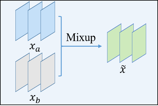
(a) Input Mixup

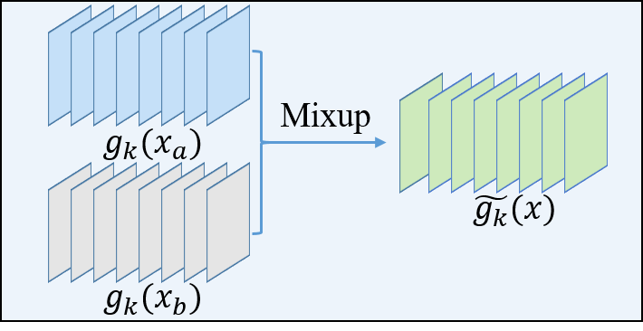
(b) Manifold Mixup

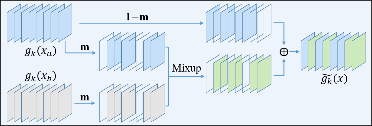
(c) ShuffleMix

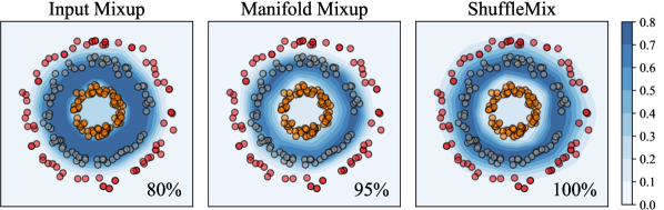
(d) Decision Boundaries

Figure 1: Comparison with the Input Mixup [10], the Manifold Mixup [12] and our Shuffle Mixup of Neural Features from Hidden Layers (ShuffleMix), where $x$ denotes the input image, $\tilde{x}$ is the mixed input image, ${g_{k}}(x)$ denotes the hidden representations of neural networks and $\tilde{g_{k}}(x)$ is the combined representation. Our ShuffleMix in (c) are more flexible than Manifold Mixup in (b), which can be viewed as a special case of our ShuffleMix. While, decision boundaries in (d) are generated based on the middle circle class for different augmentation methods on a synthetic dataset of 3-class classification. The darker the color, the higher the probability of that region belonging to the middle class. We can observe that our ShuffleMix can have smoother decision boundaries and better representation manifolds (i.e., ratio of samples falling into the darkest region) than those of the Input Mixup [10] and the Manifold Mixup [12]. Classification accuracies of three methods are shown in the bottom right of each plot. (Best viewed in colors)

Alternatively, random dropout strategies on hidden states [13] or spatial regions [14, 15] have been investigated to enforce neural models to distribute the knowledge learned from data to a large size of inter-neuron connection, rather than focusing on a limited portion. A number of recent works [16, 17, 18] have shown that introduction of random feature removal operations into representation learning as a kind of implicit network regularization can improve model generalization and representation quality. Moreover, dropout as a noise scheme can be also regarded as a form of implicit data augmentation [19], which theoretically maps the sub-regions of both input space and all high-probability natural distribution to label space. In this regard, many mixup-style data augmentation algorithms based on regional dropout have been proposed, e.g., Cutout [20], CutMix [21] and Random Erasing [22], which are able to enhance model generalization owing to discovering discriminative local features from less informative parts of object. However, these existing augmentation methods are just designed to impose the spatial attention mechanism into representation learning via regional dropout-like operations in the input space, without exploiting latent structure of representation manifolds.

The first exploration of mixup-style augmentation to feature space is the Manifold Mixup [12], which is designed on linear interpolations of hidden states of neural networks at multiple levels for smooth boundaries and flatter representations during model training. Inspired by the ShuffleNet [23], we propose a simple yet effective alternative of mixup augmentation in feature space – ShuffleMix, which favors for a channel-wise shuffle operation on feature maps from hidden layers of neural networks. Technically, a randomly-generated binary index vector $\bm{m}$ is employed for selecting channel dimensions to be shuffled in-between feature maps of two samples, which can intuitively be interpreted as a linear interpolation of feature maps after channel-wise dropout. Beyond leveraging semantically interpolated supervision signals, such a hard shuffle augmentation of hidden states can improve generalization of visual representations owing to its implicit nature of ensembling models sharing parameters as the dropout [13]. Our hard shuffle mixup can be further extended to a soft shuffle mixup via replacing a part of randomly-selected feature channels with linear interpolated features, similar to the Manifold Mixup [12]. As a result, our soft ShuffleMix can not only inherit the advantages of randomly dropout on generalization from the hard ShuffleMix, but also exploit representation manifolds in the more flexible way, as the Manifold Mixup can be considered as its special case (c.f. Section III-B for details). Comparison of the Input Mixup [10], the Manifold Mixup [12] and the proposed ShuffleMix are illustrated in Fig. 1.

Recently, superior robustness can be gained via incorporating noise injection schemes into feature interpolations of data points as the Noisy Feature Mixup (NFM) [24], which are tolerant to data perturbations in their neighboring feature space. Similarly, our ShuffleMix method can further improve representation robustness via explicitly exploring data perturbations with noise injection both in the neighbourhood of original feature maps and interpolated schemes. Experiment results on popular benchmarks of single-label and multi-label image classification tasks verify that the proposed ShuffleMix can consistently outperform existing mixup-style data augmentation methods including the state-of-the-art NFM [24].

Main contributions of this paper are as follows.

• This paper proposes a novel ShuffleMix feature augmentation method, which is simple yet generic to existing image classification networks.

• Technically, the proposed ShuffleMix is designed via a generalized linear combination of channel-wise features of a pair of randomly selected data samples, which can improve model generalization and robustness owing to its soft dropout characteristics and more flexibility to exploit representation manifolds.

• We extensively conduct experiments on several popular benchmarks of different visual classification tasks, whose results can demonstrate the effectiveness of the proposed ShuffleMix and superior performance to the state-of-the-art mixup-style augmentation methods.

Source codes and pre-trained models will be released after acceptance.

II Related work

In this section, we firstly briefly review some recent works regrading mixup style data augmentation. Secondly, existing works about implicit feature regularization in model training are investigated. Finally, we provide a brief survey about representative works in single-label and multi-label image recognition.

Mixup Style Data Augmentation – With the Mixup [10] verifying the effectiveness of data augmentation by interpolating two input images, there appears an amount of mixup style data augmentation methods [25, 11, 12, 21, 26, 27, 28, 29]. Guo et al. developed a theoretical understanding for Mixup as a kind of out-of-manifold regularization and proposed an adaptive Mixup (AdaMixup) with learnable mixing polices. Meanwhile, Yun et al. [21] proposed a CutMix augmentation strategy to blend two input images with patch-based spatial region shuffle instead of a linear interpolation. Based on the CutMix, Kim et al. [27] proposed a PuzzleMix, and Uddin et al. [28] proposed a SaliencyMix, both of which aimed to detect the representative regions for mixing with the help of saliency maps. Lee et al. [26] proposed a SmoothMix augmentation by performing the blending of two input images with a randomly generated mask for weighting instead of hard shuffle, while Huang et al. [29] proposed a SnapMix via obtaining semantic-relatedness proportion for mixed regions with the help of saliency maps. PuzzleMix [27], SaliencyMix [28], SmoothMix [26] and SnapMix [29] all are the variants of CutMix [21] with different region shuffle strategies and interpolated weights of labels. Different from above works, Verma et al. [12] proposed a Manifold Mixup augmentation strategy by extending the blending of input images to the interpolation of arbitrary hidden feature representations for imposing smooth decision boundaries, which is the direct competitor with our ShuffleMix. Recently, several more feature augmentation methods are proposed to improve representation learning, e.g., AlignMix [30] with alignment of feature tensors and Shuffle Augmentation of Features (SAF) [31] with augmenting source features from target distribution. Different from existing feature augmentation algorithms, our ShuffleMix augmentation, which can be interpreted as a kind of dropout operation, can benefit from spreading discrimination of representations to more feature dimensions, rather than overfitting on a limited size of patterns.

Implicit Feature Regularization – Regularization is generally used as an important technique to prevent over-fitting in deep learning. Except for the classical regularization methods, e.g., the Weight Decay [32], the Dropout [13] and the Batch Normalization [33], Hernandez-Garcia et al. [34] demonstrated that data augmentation can be treated as an implicit regularization, which can perform better than those classical regularization for model training. More works explored different type of dropout for regularizing convolutional networks, including the DropBlock [15] and the Weighted Channel Dropout [35]. Specially, traditional dropout style methods are all regularizing the input images and features by replacing some spatial regions or dimensions with zero, which suffers from losing important information. Carratino et al. [36] and Zhang et al. [37] further analyzed that Mixup [10] can help to improve the performance of models as a specific regularization based on the Taylor approximation. Inspired by such an observation, the proposed ShuffleMix can be considered as complementing mixup augmentation with a dropout like operation as implicit feature regularization in a unified framework.

Single-Label Visual Classification – The problem of single-label image recognition has been actively studied for decades. Existing works are generally categorized into part-based methods [38, 39, 40] and part-free methods [2, 3, 4, 41, 42, 43, 44]. Part-based methods usually attempt to learn critical information from detected key parts region of objects for fine-grained recognition. Huang et al. [38] proposed a Part-Stacked CNN for learning distinguished information via modeling the subtle differences between objects parts. To better locate the object parts, Zheng et al. [40] proposed a progressive-attention CNN to locate object parts with varying scale. Unlike part-based methods, part-free methods always focus on extracting discriminative features from global region via exploiting training strategies or network constraints. Du et al. [41] proposed a progressive training strategy and a jigsaw puzzle operation to exploit multi-granularity features learning. Shi et al. [43] attempted to exploit hierarchical label structure of fine-grained classes by leveraging a cascaded softmax loss and a generalized large-margin loss. Ding et al. [44] proposed an attention pyramid CNN to enhance feature representation by integrating cross-level feature information. Our ShuffleMix aims to enhance model generalization via implicit regularization on representation learning, with combining both mixup style augmentation and dropout operations in a unified framework, which can thus be readily adopted in existing classification networks.

Multi-Label Visual Classification – Compared with typical single-label image classification, the problem of multi-label classification [45, 46] is more challenging in view of complicated object co-occurrence in the images, which leads to large variations of visual representations. With the rise of deep networks [4, 47], most recent works [6, 48, 49, 50, 51, 52, 53] tend to address the problem via deep representation learning and a multi-label classification layer to model latent correlation across targets. Wang et al. [54] developed a recurrent memorized-attention module contained with a spatial transformer layer and a LSTM unit for capturing the correlation between local and global regions. Chen et al. [6] introduced Graph Convolutional Networks (GCN) into popular deep model to learn the label correlation with an end-to-end trainable way. Recently, Wen et al. [53] proposed a feature and label co-projection (CoP) module to explicitly model the context of multi-label images, inspired by the psychological way of human recognizing multiple objects simultaneously. Although those algorithms with pre-trained deep networks can alleviate the problem of multi-label classification task, there are still suffer from lack of sufficient training data to model cross-object dependency. Our method can vastly augment more training samples in the feature space with mixed multi-labels to alleviate the challenge as well as better generalization.

III Methodology

In Sec. III-A, we firstly introduce some notations used in this paper as well as several representative mixup style data augmentation methods, i.e., the Mixup [10] and the Manifold Mixup [12]. Secondly, the proposed ShuffleMix method is presented in Sec. III-B. Finally, we combine our ShuffleMix with the Noisy Injection scheme in Sec. III-C.

III-A Preliminaries

In supervised single-label classification (e.g., general image classification [2, 3, 4] and fine-grained image classification [38, 39, 40, 41, 42, 43, 44]), given a training data set ${\{(x_{i},y_{i})\}_{i=1}^{N}}$, the model $f(x)$, e.g., a deep neural network, is usually trained by minimizing the empirical risk (ERM):

$$R(f)=\frac{1}{N}\sum_{i=1}^{N}\ell(f(x_{i}),y_{i}),$$ (1)

where $x_{i}\in\mathbb{R}^{W\times H\times C}$ denotes the $i$-th input image with width $W$, height $H$ and color channels $C$, $y_{i}$ denotes the corresponding label, and $\ell(\cdot)$ is the loss function, e.g., the typical cross entropy loss. To improve model generalization, there appears a series of mixup style data augmentation, e.g., Mixup [10] and Manifold Mixup [12].

The vanilla Mixup [10] method generates a new interpolated image $\tilde{x}$ and correspondingly semantically interpolated label $\tilde{y}$ by combining any two training images $(x_{a},y_{a})$ and $(x_{b},y_{b})$ with a random trade-off value $\lambda$, which can be written as follows:

$$\tilde{x}=\lambda x_{a}+(1-\lambda)x_{b},$$ (2)

$$\tilde{y}=\lambda y_{a}+(1-\lambda)y_{b},$$

where $\lambda\thicksim Beta(\alpha,\alpha)$, for $\alpha\in(0,+\infty)$. When $\alpha$ is set to 1, the value of $\lambda$ is the same as sampling from a uniform distribution $U(0,1)$. The generated image $\tilde{x}$ is used to train the model $f(x)$, supervised by the interpolated label $\tilde{y}$.

Recently, the Manifold Mixup [12] is proposed to leverage interpolations in deeper hidden layers rather than only in the input space for exploiting manifolds of high-level representations. We train deep image classifiers with the Manifold Mixup based data augmentation with the following steps.

• First, supposing a model $f(x)=f_{k}\circ g_{k}(x)$, where $g_{k}$ denotes the shallow $k$ feature encoding layers and $f_{k}$ denotes all the remaining ones. The $g_{k}(x)\in\mathbb{R}^{W^{\prime}\times H^{\prime}\times C^{\prime}}$ represents the hidden representation at layer $k$, where $k$ is randomly selected from a range of eligible layers $\mathcal{S}=\{k\}$ in the whole classification network.

• Second, the interpolated representation $\tilde{g_{k}}(x)$ is generated by performing the vanilla Mixup [10] on two random hidden representations $g_{k}(x_{a})$ and $g_{k}(x_{b})$, which are encoded from training images $(x_{a},y_{a})$ and $(x_{b},y_{b})$ respectively, with a random value $\lambda$, illustrated as follows:

  $$\tilde{g_{k}}(x)=\lambda g_{k}(x_{a})+(1-\lambda)g_{k}(x_{b}),$$ (3)

  where $k\in\mathcal{S}$, $\lambda\thicksim Beta(\alpha,\alpha)$ and the corresponding semantically interpolated label $\tilde{y}=\lambda y_{a}+(1-\lambda)y_{b}$.

• Third, the generated representation $\tilde{g_{k}}(x)$ is used to additionally train the model $f_{k}(\tilde{g_{k}}(x))$ under supervision of $\tilde{y}$. Note that, the Manifold Mixup [12] in the case where $\mathcal{S}=\{0\}$, is equivalent to the vanilla Mixup [10].

III-B Shuffle Mixup of Neural Hidden States

As the hidden representations in the middle layers preserving low-dimensional manifolds, feature interpolations of different category samples introduced by the Manifold Mixup [12] are enforced to avoid label inconsistency for the same augmented data point with different original sample pairs by flattening their features, which can thus improve model generalization via increasing margins to smoother decision boundaries. As mentioned in Sec. I, simple linear operations are not limited to the linear interpolation in the Manifold Mixup [12], which encourage us to use a generalized linear combination to more flexibly extend the capacity of representations constrained by low-dimensional manifolds.

Motivated by the efficient ShuffleNet [23], this paper proposes the ShuffleMix method, which favors channel-wise linear operations such as interpolation and shuffle on feature maps. Specifically, our ShuffleMix can preserve a part of feature channels, while the rest of maps perform the typical interpolation as other mixup methods on two random hidden representations at the same indices. The advantages of our ShuffleMix are summarized in four folds below.

• Our ShuffleMix is a generalized scheme to allow the vanilla Mixup and the Manifold Mixup as its special cases.

• Feature channels randomly selected for mixup can be considered as soft dropout regularization to improve model generalization (see results in Sec. V-B).

• Ratio of the preserved feature maps can control perturbation boundary of the augmented features as an implicit smoothness regularization to improve model robustness against noises (see results in Sec. V-C).

• Feature mixing between different samples can vastly improve representations not only for single-label classification (see Sec. V-B), but also for multi-label classification (see Sec. V-E).

Training the model $f(x)$ with our ShuffleMix are largely similar to the Manifold Mixup, while the main difference lies in the second step, where our ShuffleMix allows not only feature interpolation but also channel-wise shuffle operation on feature maps from hidden layers of neural networks. Especially, a randomly-generated binary index vector $\bm{m}$ is employed for selecting channel dimensions to be shuffled in-between feature maps of two samples, which can be formulated into the following equation:

$$\tilde{g_{k}}(x)=(\mathbf{1}-\mathbf{m})\ \odot\ g_{k}(x_{a})+\mathbf{m}\ \odot\ g_{k}(x_{b}),$$ (4)

where $\mathbf{m}\in\{0,1\}^{C^{\prime}}$ denotes a binary index along the channel dimension for indicating which channel need to be performed with a linear interpolation of channel-wise dropout feature maps, $\mathbf{1}$ is a binary vector filled with all one elements, and $\odot$ denotes channel-wise multiplication.

Compared with the Manifold Mixup in Eq. (3), our proposed ShuffleMix operation in Eq. (4) plays a hard shuffle mixup of hidden states instead of leveraging linear mixup between feature maps of two samples. To make our ShuffleMix more flexible, we further extended the hard shuffle mixup to a soft shuffle mixup via replacing a part of randomly-selected feature channels with mixup interpolated features. The formula can be depicted as follows:

$$\tilde{g_{k}}(x) =(\mathbf{1}-\mathbf{m})\ \odot\ g_{k}(x_{a})$$ (5)

$$+\mathbf{m}\ \odot\ \{\lambda g_{k}(x_{a})+(1-\lambda)g_{k}(x_{b})\},$$

where $\lambda$ is a random value sampled from the beta distribution $Beta(\alpha,\alpha)$ like the vanilla Mixup [10]. We define such an operation in Eq. (5) with $\lambda\thicksim Beta(\alpha,\alpha)$ as soft ShuffleMix, while the operation in Eq. (4) is named as hard ShuffleMix, easily degenerated from soft ShuffleMix with $\lambda\cong 0$. Performance comparisons between soft and hard ShuffleMix are shown in the experiment part. Unless particularly stated, the results of our ShuffleMix in the experiments are obtained with the soft ShuffleMix. The binary index $\mathbf{m}$ is actually a $C^{\prime}$-dimensional vector, whose sum $||\mathbf{m}||$ indicates the number of indexed channels. Given a hyper parameter $r\in(0,1]$ for representing the ratio of indexed channels, we can obtain $||\mathbf{m}||=|r*C^{\prime}|$. Note that, $r$ should be larger than zero, and when $r=1$, our ShuffleMix is equivalent to the Manifold Mixup [12]. Given $\lambda$ and $r$, we can calculate the semantically interpolated label $\tilde{y}$ as the following:

$$\tilde{y}=(1-r)y_{a}+r\{\lambda y_{a}+(1-\lambda)y_{b}\}.$$ (6)

It is worth mentioning here that with an appropriate $r$, augmented features can always fall into the sample $x_{a}$’s neighborhood, which can be viewed as implicitly incorporating data perturbation, similar to the Noisy Feature Mixup [24] (see Sec. III-C).

Algorithm 1 The pipeline of our ShuffleMix

0:  Dataset $\mathcal{D}_{train}$ and $\mathcal{D}_{test}$, model $f(x)=f_{k}\circ g_{k}(x)$, eligible layers $\mathcal{S}=\{k\}$, ratio $r$, hyper-parameter $\alpha$.

0:  Predicted output $\hat{y}$

1:  if training then

2:     Random sample a batch of training data $\mathcal{B}\subset\mathcal{D}_{train}$

3:     for $i=1$ to $|\mathcal{B}|$ do

4:        Random generate a value $\lambda$ with $Beta(\alpha,\alpha)$

5:        Random select a number k from layers $\mathcal{S}$ for hooking hidden representation

6:        Generate random binary index $\mathbf{m}$ with ratio r

7:        Obtain hidden representation $g_{k}(x_{i})$ at k layer

8:        Generate mixed feature $\tilde{g_{k}}(x_{i})$ by Eq.(5)

9:        Generate mixed label $\tilde{y_{i}}$ by Eq.(6)

10:        Obtain the predicted output $\hat{y}$ with $f_{k}\circ\tilde{g_{k}}(x_{i})$

11:     end for

12:     Compute the empirical risk according to Eq.(1)

13:     Backward to update the parameters of the model

14:  else

15:     Random sampling testing data $x\subset\mathcal{D}_{test}$

16:     Compute the predicted output $\hat{y}=f(x)$

17:  end if

18:  return  $\hat{y}$

As shown in Eq. (4) and Eq. (5), the operation $\odot$ can be implemented simply with a way of channel replacement in practice, while the replacement operation is theoretically cost-free. Hence, our ShuffleMix algorithm has the same computational and space complexity as that of the Manifold Mixup [12] algorithm, which can be also verified by our experiments. The detailed training processing of our ShuffleMix is presented in Algorithm 1.

III-C Combining with Noisy Feature Mixup

The Noisy Feature Mixup (NFM) [24] was recently proposed to use the Manifold Mixup [12] by injecting additive and multiplicative noises into the interpolated representations $\tilde{g_{k}}(x)$ in Eq. (3) as feature regularization, which can be depicted as:

$$\tilde{g_{k}}(x)_{\text{NFM}}=(1+\delta_{mult}\xi_{k}^{mult})\odot\tilde{g_{k}}(x)+\delta_{add}\xi_{k}^{add},$$ (7)

where $\delta_{mult}$ and $\delta_{add}$ are pre-defined hyper parameters for leveling additive noise $\xi_{k}^{mult}$ and multiplicative noise $\xi_{k}^{add}$ respectively. As mentioned in NFM [24], $\xi_{k}^{mult}$ and $\xi_{k}^{add}$ are independent random variables, which are sampled from a normal distribution and a uniform distribution for approximating white and salt & pepper noises respectively. Other training details are kept the same as that in the Manifold Mixup [12].

Motivated by performance gain by the combination of mixup style data augmentation and noise injection, we similarly train deep representation learning with combining our ShuffleMix and noisy feature injection. This method named as ShuffleMix-NFM based on Eq. (7) replaces the interpolated representation $\tilde{g_{k}}(x)$ of the Manifold Mixup [12] with those of our ShuffleMix in Eq. (5).

As illustrated in Eq. (5) and Eq. (4), the interpolated representation $\tilde{g_{k}}(x)$ in our ShuffleMix not only contains interpolated features, but also preserves original ones. Therefore, combination of $\tilde{g_{k}}(x)$ in our ShuffleMix and injected noises in Eq. (7) can achieve superior robustness owing to data perturbation on both raw and mixed representations, rather than only the latter in the manifold mixup, which is supported by experimental results in Sec. V-B.

IV Adaptation to Multi-Label Classification

To further illustrate the effectiveness of our proposed methods, we adapt our method to multi-label classification, which was originally designed for single-label image classification. The challenge in multi-label representation lies in more complicated label dependency, which leads to large variations of visual representations, in comparison with single-label classification. This task commonly train a multi-label classifier $f(\cdot)$ on the training set ${\{(x_{i},y_{i})\}_{i=1}^{N}}$ with multi-label binary cross-entropy loss as follows:

$$\ell(\cdot)=\sum_{k=1}^{K}-y_{i}^{k}\log(\sigma(\hat{y_{i}}^{k}))-(1-y_{i}^{k})\log(1-\sigma(\hat{y_{i}}^{k})),$$ (8)

where $K$ denotes the number of labels, $y_{i}\in{\{0,1\}}^{K}$ denotes the target multi labels, $\hat{y_{i}}=f(x_{i})$ denotes the predicted multi labels, and $\sigma(\cdot)$ denotes the sigmoid function.

Considering the target labels of binary cross-entropy loss in Eq. (8) are always either zero or one, we can’t directly apply the ShuffleMix with soft labels $\tilde{y}$ in Eq. (6) for multi-label classification. For the ShuffleMix data augmentation in Eq. (5), a straightforward solution is to set values of soft labels greater than zero to be one. However, such an approximation will introduce external label noises for those subtle label values. For focusing on the dominant targets in multi-label data augmentation, we introduce a pre-defined threshold $m$ for soft labels $\tilde{y}$ as follows:

$$\tilde{y}_{t}=\left\{\begin{array}[]{rcl}1&\text{if}\ \tilde{y}\geq m\\ 0&\text{otherwise},\end{array}\right.$$ (9)

where $\tilde{y}\in\mathbb{R}^{K}$, $\tilde{y}_{t}\in{\{0,1\}}^{K}$. Therefore, we can employ the adjusted binary labels $\tilde{y}_{t}$ to train classification models with the loss function in Eq. (8) for feature augmentation for multi-label classification. The optimal value of $m$ will be determined empirically, whose ablation studies are shown in the experiments. To our best knowledge, our work is the first attempt to apply mixup augmentation to multi-label classification, and experiment results in Sec. V-E can verify the effectiveness of our ShuffleMix for multi-label classification.

V Experiments

In this section, we empirically validate the proposed ShuffleMix algorithm on popular benchmarks of single-label visual classification tasks, i.e., public benchmarks of general image classification, i.e., the CIFAR [55] and the Tiny ImageNet [56], and three fine-grained datasets including the CUB-200-2011 (CUB) [57], the Stanford Cars (CAR) [58] and the FGVC Aircraft (AIR) [59]. Furthermore, the ShuffleMix is adapted to the multi-label classification task on the Pascal VOC 2007 dataset [60]. Finally, visualizations of decision boundaries of different methods are compared for better understanding.

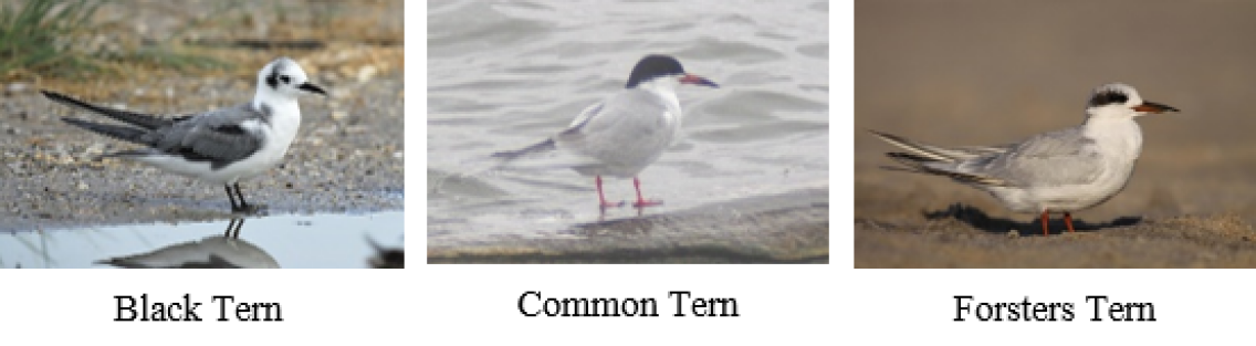
(a) Single-label samples from the CUB-200-2011

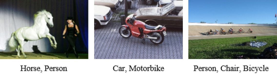
(b) Multi-label samples from the PASCAL VOC 2007

Figure 2: Examples from the CUB-200-2011 [57] and the PASCAL VOC 2007 [60] datasets. The category labels corresponding to the images are displayed below the image. The single-label samples generally just contain one object, while those for multi-label classification usually contains more scene objects.

V-A Datasets and Settings

Datasets – We conduct experiments on three widely used datasets: the CIFAR-10 [55], the CIFAR-100 [55] and the Tiny ImageNet [56] for general image classification. Specifically, the CIFAR-10 and the CIFAR-100 datasets both contain 50,000 training images and 10,000 test images, belonging to 10 and 100 semantic object classes respectively, while the Tiny ImageNet consists of 100,000 training images of 200 classes and 10,000 test images. Note that, both CIFAR and Tiny ImageNet datasets have a balanced distribution for both training and test sets. For the fine-grained classification task, we conduct experiments on three widely used fine-grained datasets, namely the CUB-200-2011 (CUB) [57], the Stanford Cars (CAR) [58] and the FGVC Aircraft (AIR) [59]. The details of datasets are provided in Table I, where we only use the category labels as supervision signals without any additional prior information.

TABLE I: Statistics of three fine-grained datasets.

Dataset	Classes	Training data	Testing data
CUB [57]	200	5,994	5,794
CAR [58]	196	8,144	8,041
AIR [59]	100	6,667	3,333

Comparative Methods – To better evaluate the generalization of our method, we conduct experiments by employing three varieties of the ResNet [4], i.e., PreActResNet18, PreActResNet34 and Wide-PreActResNet18-2, which are also adopted in our direct competitors – the Manifold mixup [12] and the NFM [24]. Following [12, 24], we use the three networks just with ERM as the baseline. We compare our method with typical Dropout [13] regularization and representative mixup style data augmentation methods, i.e., Input Mixup [10] and Manifold Mixup [12]. On evaluation about robustness against noises, the state-of-the art NFM [24] is competed with the ShuffleMix method.

Implementation Details – In all our experiments for general image classification, we adopt stochastic gradient descent (SGD) with momentum of 0.9 and a weight decay of $5\times 10^{-4}$ for training models. Following implementation details in [24], all our experiments are trained for 200 epochs with a batch size of 128 and a step-wise learning rate decay. The initial learning rate is set as 0.1 and then decayed with a factor of 0.1 at the 100-th epoch, the 150-th epoch and the 180-th epoch, respectively. In Eq. (5), there are three hyper parameters, i.e., $\alpha$ for beta distribution, $r$ for the ratio of indexed channels for mixup and $\mathcal{S}$ for the range of eligible layers. Unless particularly stated, we empirically set $\alpha=1$, $r=0.5$ and $\mathcal{S}=\{0,1,2,3,4\}$ in our experiments. For fine-grained image classification, we prepare data and implement model training by following the same setting in [29, 42]. The hyper-parameters of the ShuffleMix are setting as same as that in general image classification. For fair comparison, we keep the same training setting for all fine-grained experiments. For the evaluation on model robustness, there are another two hyper parameters $\delta_{add}$ and $\delta_{mult}$ for controlling the level of additive noise and multiplication noise, respectively. We set $\delta_{add}=0.2$ and $\delta_{mult}=0.4$ in the experiments by following the same setting as [24]. To compare with Dropout regularization, we apply Dropout between the final FC layer and feature extractor of each network with a dropping rate of 0.2. The parameters in Mixup and Manifold Mixup are following that in [10, 12]. We implement and train the models in all experiments with the Pytorch [61] library based on a single NVIDIA 1080ti GPU.

TABLE II: Comparative evaluation with classification accuracy using three backbone networks on the CIFAR-10 and the CIFAR-100. Standard deviations are obtained over three trails.

PreActResNet18	CIFAR-10 (%)	CIFAR-100 (%)
Baseline	94.69 $\pm$ 0.172	76.12 $\pm$ 0.180
Dropout [13]	94.63 $\pm$ 0.102	76.17 $\pm$ 0.195
Input Mixup [10]	95.67 $\pm$ 0.140	79.32 $\pm$ 0.302
Manifold Mixup [12]	95.66 $\pm$ 0.066	79.33 $\pm$ 0.249
ShuffleMix (Ours)	95.78 $\pm$ 0.154	80.02 $\pm$ 0.163
PreActResNet34
Baseline	94.74 $\pm$ 0.125	76.36 $\pm$ 0.189
Dropout [13]	94.72 $\pm$ 0.131	76.17 $\pm$ 0.152
Input Mixup [10]	95.78 $\pm$ 0.103	79.54 $\pm$ 0.323
Manifold Mixup [12]	95.57 $\pm$ 0.155	79.87 $\pm$ 0.083
ShuffleMix (Ours)	95.78 $\pm$ 0.097	80.53 $\pm$ 0.118
Wide-PreActResNet18-2
Baseline	94.95 $\pm$ 0.040	76.90 $\pm$ 0.099
Dropout [13]	94.87 $\pm$ 0.167	77.09 $\pm$ 0.142
Input Mixup [10]	96.07 $\pm$ 0.019	81.07 $\pm$ 0.039
Manifold Mixup [12]	95.82 $\pm$ 0.025	80.46 $\pm$ 0.311
ShuffleMix (Ours)	96.36 $\pm$ 0.037	81.96 $\pm$ 0.159

V-B Evaluation on Single-Label Image Classification

Evaluation on General Image Classification – As mentioned in Sec. V-A, we conduct experiments on the CIFAR-10 and the CIFAR-100 with PreActResNet18, PreActResNet34 and Wide-PreActResNet18-2 backbone networks, respectively. Comparative results are reported in Table II, where all methods are under the identical experimental settings. Evidently, the ShuffleMix method can consistently achieve the superior accuracy to comparative mixup style data augmentation methods as well as the baseline, with three backbone networks on both datasets. Note that, our method outperforms its direct competitor – the Manifold Mixup, which is limited to linear interpolations of hidden representations. Superior performance of the ShuffleMix can be explained by the only difference between both methods lying in the introduction of a more flexible linear combinational operation, which thus can demonstrate our claim.

Evaluation on Large-Scale Data – To verify generalization of our method on large-scale data, another experiment on the Tiny ImageNet is conducted with using PreActResNet18, PreActResNet34 and Wide-PreActResNet18-2 backbone networks. Results of competing methods are compared in Table III, where we can find out that the proposed ShuffleMix can outperform the Baseline by 2.78%, 4.56 and 3.04% on top-1 accuracy when using PreActResNet18, PreActResNet34 and Wide-PreActResNet18-2 backbones, respectively. Meanwhile, the result of our ShuffleMix can beat the Manifold Mixup [12] by 1.17%, 0.8% and 1.66% on top-1 accuracy when using PreActResNet18, PreActResNet34 and Wide-PreActResNet18-2 backbone, respectively. Similar results can also be observed when using top-5 accuracy as performance metric. Experiment results on the Tiny ImageNet again verify the effectiveness of our method on large-scale data.

TABLE III: Comparative evaluation with classification accuracy using three backbone networks on the Tiny ImageNet.

PreActResNet18	top-1 (%)	top-5 (%)
Baseline	62.64	83.05
Dropout[13]	62.46	82.64
Input Mixup [10]	64.47	84.02
Manifold Mixup [12]	64.25	84.38
ShuffleMix (Ours)	65.42	85.10
PreActResNet34
Baseline	62.06	82.83
Dropout [13]	61.59	81.50
Input Mixup [10]	64.39	84.59
Manifold Mixup [12]	65.81	85.62
ShuffleMix (Ours)	66.61	85.84
Wide-PreActResNet18-2
Baseline	64.76	83.40
Dropout [13]	64.40	84.74
Input Mixup [10]	65.24	84.15
Manifold Mixup [12]	66.14	84.86
ShuffleMix (Ours)	67.80	85.76

Evaluation on Fine-Grained Image Classification – The accuracy results on three fine-grained datasets are reported in Table IV, where we employ two different backbones, i.e., ResNet34 [4] and ResNet50 [4]. Experiments results demonstrate that the ShuffleMix can also better improve the classification performance than Mixup [10] and Manifold Mixup[12] on fine-grained datasets, which indicates that the proposed ShuffleMix can also benefit the learning of fine-grained classification. Especially, our ShuffleMix with ResNet34 backbone on AIR [59] dataset can outperform the baseline by near 2%.

TABLE IV: Comparison with classification accuracy using ResNet34 and ResNet50 backbones on the CUB-200-2011 (CUB), the Stanford Cars (CAR), and the FGVC-Aircraft (AIR) benchmarks.

ResNet34	CUB (%)	CAR (%)	AIR (%)
Baseline	84.83	91.94	89.98
Input Mixup [10]	84.74	92.76	90.49
Manifold Mixup[12]	85.24	92.91	90.70
ShuffleMix (Ours)	85.90	93.33	91.96
ResNet50
Baseline	85.46	92.89	90.97
Input Mixup [10]	85.98	93.35	90.94
Manifold Mixup [12]	86.29	93.88	92.08
ShuffleMix (Ours)	87.00	94.12	92.41

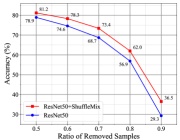
(a) CUB

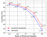
(b) CAR

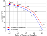
(c) AIR

Figure 3: Classification performance on different fine-grained datasets under varying sample size of each class. (Best viewed in colors)

TABLE V: Robustness of comparative methods based on PreActResNet18 and Wide-PreActResNet18-2 backbones, w.r.t. white noise ($\delta$) and salt and pepper ($\gamma$) perturbations on the CIFAR-100. The best results are marked in bold, and the second best results are marked in lavender background. Results are averaged over three trials.

Methods	Clean (%)	$\delta$ (%)			$\gamma$ (%)
		0.1	0.2	0.3	0.02	0.04	0.1
PreActResNet18
Baseline	76.12	56.90	29.20	14.07	59.04	41.56	16.07
Input Mixup [10]	79.32	65.66	39.77	19.37	58.80	40.00	15.39
Manifold Mixup [12]	79.33	63.98	33.64	15.42	63.23	45.71	15.33
ShuffleMix (Ours)	80.02	67.03	43.05	21.68	70.72	60.88	35.96
NFM [24]	79.15	75.07	57.22	33.84	70.20	59.87	31.46
ShuffleMix-NFM (Ours)	79.67	76.45	61.79	40.45	72.94	66.12	44.42
Wide-PreActResNet18-2
Baseline	76.90	56.44	27.07	12.73	58.50	39.99	14.89
Input Mixup [10]	81.07	67.88	42.53	22.25	62.32	42.58	15.65
Manifold Mixup [12]	80.46	63.40	30.35	13.48	63.09	44.03	15.46
ShuffleMix (Ours)	81.96	70.09	43.74	21.03	70.81	58.29	31.83
NFM [24]	81.20	78.03	61.73	37.05	73.02	63.16	33.60
ShuffleMix-NFM (Ours)	81.58	78.67	64.42	42.57	75.83	69.20	48.77

V-C Robustness Evaluation

Robustness Against Noises – To verify the robustness of our method ShuffleMix and its extension ShuffleMix-NFM, experiments with different input perturbations, i.e., white noise or salt and pepper noise, are conducted. Specifically, on the CIFAR-100, the Baseline and other mixup style data augmentation methods, i.e., Input Mixup [10], Manifold Mixup [12] and NFM [24] are compared with our methods with the same settings mentioned in Sec. V-A. Results shown in Tables V are based on the backbones PreActResNet18 and Wide-PreActResNet18-2, respectively. Results with training models with noise-free data are reported in the first block of both tables, while the Clean indicates that the test data without any perturbation. $\delta$ and $\gamma$ are used to control the level of white noise and salt & pepper noise. Evidently, as illustrated in both tables, it is found out that the ShuffleMix can consistently achieve the best performance on the Clean testing data and also perform more robustly to two types of noises. For a fair comparison with the state-of-the-art NFM method [24], we train the ShuffleMix-NFM with the same settings as the NFM, whose results are illustrated in the bottom block of Table V with two different backbones on the CIFAR-100. The proposed ShuffleMix-NFM can further improve the robustness of models than the ShuffleMix and the NFM [24] with significant margins. More results about robustness against input perturbations on the Wide-PreActResNet18-2 are illustrated in Fig. 4. The results here can support our claim about improving model robustness via allowing data perturbation in feature space as an implicit regularization.

Robustness Against Data Sparsity – We further apply the ShuffleMix with varying sparse training samples to verify the robustness against sparse data distribution. As both training and test sets are near balanced distributed of datasets in Table I, we set the sparsity of training sets with a limited size of samples for each class (i.e., removing 50% to 90% of training samples), whereas the whole validation set is adopted in our experiments. As shown in Fig. 3, our ShuffleMix can always achieve superior results under varying sparsity on different fine-grained datasets, which show our ShuffleMix is more robust against sparse data.

TABLE VI: Classification accuracy of hard and soft ShuffleMix for varying $r$ on the CIFAR-100 with PreActResNet18 backbone.

ratio $r$	0.125	0.25	0.375	0.5	0.625	0.75	0.875
hard ShuffleMix $\lambda\cong 0$	78.90	79.05	79.92	78.87	79.83	79.45	78.81
soft ShuffleMix $\lambda\thicksim Beta(1,1)$	78.49	78.82	79.38	80.02	79.63	79.56	79.46

TABLE VII: Effects of different $\alpha$ in the proposed ShuffleMix on the CIFAR-100 with PreActResNet18 backbone. The best results in every column are marked in bold.

$\alpha$	0.5	1	2	4	8
Input Mixup [10]	79.32	79.32	77.95	76.50	75.33
Manifold Mixup [12]	79.18	79.33	79.26	78.42	77.75
ShuffleMix (Ours)	79.75	80.02	79.60	79.34	79.22

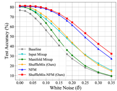
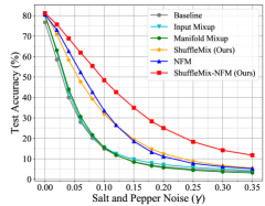
Figure 4: Robustness of comparative methods based on the Wide-PreActResNet18-2 backbone on the CIFAR-100 with classification accuracy. We repeat the experiments for five times to generate the mean accuracy. (Best viewed in color)

V-D Ablation Studies

As aforementioned, all the experiments are conducted on our soft ShuffleMix method by using the same hyper parameters. To further compare the difference between our soft ShuffleMix in Eq. (5) and hard ShuffleMix in Eq. (4), we jointly conduct ablation studies about the hyper parameter $r$ for controlling the ratio of indexed channels for shuffle mixup on model generalization, with our hard and soft ShuffleMix methods, respectively. Experiment results are presented in VI, where the hyper parameter $\alpha$ in soft ShuffleMix is set as 1, and the $\lambda\cong 0$ is fixed for hard ShuffleMix. It is observed that when $r=0.5$ in our soft ShuffleMix and $r=0.375$ in our hard ShuffleMix, we can achieve the best performance, which both suggests an appropriate $r$ for good performance, while the remaining options of $r$ can still perform better than comparative methods in Table II. Specifically, the result of $r=0.5$ in soft ShuffleMix shows that we can get the best performance when we choose half of random indexed channels to do mixup interpolation, which may be benefited from soft dropout via a generalized linear combination of feature maps. Similarly, the best results in hard ShuffleMix can be achieved when we perform channel-wise shuffle operation on feature maps with more or less half of random indexed channels, e.g., $r=0.375$ and $r=0.625$. Such performance comparisons again show that our soft ShuffleMix is more flexible than hard ShuffleMix. Effects of hyper parameter $\alpha$ are also investigated in Table VII with $r=0.5$ for our soft ShuffleMix, whose $\lambda\thicksim Beta(\alpha,\alpha)$. We observe that the variation of $\alpha$ can make very marginal effects on our method, while the other comparative data augmentation methods are sensitive to the value of $\alpha$. We conclude that in the proposed ShuffleMix, $r$ is more sensitive than $\alpha$ to classification performance, which confirm that preservation of a part of features is the key factor of our design owing to its nature of soft dropout on improving generalization.

TABLE VIII: Comparison evaluation of AP and mAP on the PASCAL VOC 2007 dataset. The sign of “*” indicates the re-implemented results via running the source code from the original authors. The ResNet101 model is slightly modified with a global max-pooling after the last layer. The best results are marked in bold, and the second best results are marked in lavender background.

Methods	aero	bike	bird	boat	bottle	bus	car	cat	chair	cow	table	dog	horse	motor	person	plant	sheep	sofa	train	tv	mAP
HCP [62]	98.6	97.1	98.0	95.6	75.3	94.7	95.8	97.3	73.1	90.2	80.0	97.3	96.1	94.9	96.3	78.3	94.7	76.2	97.9	91.5	90.9
RCP [63]	99.3	97.6	98.0	96.4	79.3	93.8	96.6	97.1	78.0	88.7	87.1	97.1	96.3	95.4	99.1	82.1	93.6	82.2	98.4	92.8	92.5
RDAR [54]	98.6	97.4	96.3	96.2	75.2	92.4	96.5	97.1	76.5	92.0	87.7	96.8	97.5	93.8	98.5	81.6	93.7	82.8	98.6	89.3	91.9
RARL [51]	98.6	97.1	97.1	95.5	75.6	92.8	96.8	97.3	78.3	92.2	87.6	96.9	96.5	93.6	98.5	81.6	93.1	83.2	98.5	89.3	92.0
CoP [53]	99.9	98.4	97.8	98.8	81.2	93.7	97.1	98.4	82.7	94.6	87.1	98.1	97.6	96.2	98.8	83.2	96.2	84.7	99.1	93.5	93.8
ML-GCN [6]	99.5	98.5	98.6	98.1	80.8	94.6	97.2	98.2	82.3	95.7	86.4	98.2	98.4	96.7	99.0	84.7	96.7	84.3	98.9	93.7	94.0
ResNet101* [4]	99.8	98.3	98.4	98.3	79.4	93.4	97.2	97.6	79.5	93.7	86.5	97.8	97.9	96.2	98.7	84.0	95.8	79.8	98.7	93.3	93.2
ResNet101+ShuffleMix	99.5	98.5	98.3	98.5	81.5	96.0	97.7	98.3	83.3	96.9	87.1	98.3	98.5	96.0	99.1	86.3	96.7	86.7	98.9	94.8	94.5
ML-GCN* [6]	99.8	98.3	98.7	98.2	80.3	94.6	97.3	97.8	81.1	94.9	87.2	97.9	98.0	95.8	98.8	82.7	95.8	82.1	98.6	93.1	93.5
ML-GCN+ShuffleMix	99.4	99.0	98.7	98.5	81.6	95.6	97.8	98.4	83.6	96.9	88.2	98.5	98.7	96.8	99.0	84.9	97.2	85.2	99.3	95.3	94.6

TABLE IX: Effects of different threshold m in the proposed ShuffleMix for multi-label classification on the PASCAL VOC 2007 with ResNet101 and ML-GCN backbone.

threshold (m) =	0.1	0.2	0.3	0.4	0.5
ResNet101+ShuffleMix	94.33	94.54	94.38	94.45	94.13
ML-GCN+ShuffleMix	94.08	94.30	94.62	94.63	94.32

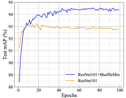
Figure 5: The test mAP of the ShuffleMix and corresponding networks on the PASCAL VOC 2007 along training epochs. (Best viewed in color)

V-E Evaluation on Multi-Label Image Classification

As the ShuffleMix augments training samples by combining two sampled features during training, it can also be used to improve the representation learning for multi-label classification, as long as the features are similarly trained from the network backbone. To demonstrate that, we apply the ShuffleMix to the multi-label classification task on the PASCAL VOC 2007 dataset [60], which contains 5,011 training images and 4,952 testing images from 20 categories. As showed in Fig. 2(b), each image from the PASCAL VOC 2007 usually contains several different categories of objects. We follow the same experiment settings in the ML-GCN [6] and implement the ShuffleMix algorithm with ResNet-101 [4] and ML-GCN [6] networks, respectively. Motivated by the ML-GCN [6], the ResNet-101 used here is slightly modified by replacing with a global max-pooling after the last layer, which can help the network get better performance. To compare with other related works, we report the results with the average precision (AP) of each category and the mean average precision (mAP) of all categories. The hyper-parameters $\alpha=1$, $r=0.5$ and $\mathcal{S}=\{0,1,2,3,4\}$ in the ShuffleMix are set as usual like that stated in Sec. V-A, and the parameter $m$ in Eq. (9) will be studied in ablation studies.

The results on the PASCAL VOC 2007 benchmark are reported in Table VIII, where we reproduced the results of ResNet-101 [4] and ML-GCN [6] under the same experiment settings for a fair comparison. It is obvious that the proposed ShuffleMix can improve the performance significantly even with different backbone networks for multi-label classification. Concretely, the proposed ShuffleMix with corresponding networks can outperform the ResNet-101 by 1.3% mAP and the ML-GCN by 1.1% mAP, respectively. It’s worth noting that the proposed ShuffleMix with ML-GCN network can obtain 94.6% mAP, while even with ResNet-101 network, our ShuffleMix can achieve 94.5% mAP.

As illustrated in Fig. 5, we can find out that the test mAP of our ShuffleMix with baseline networks can be continuously improved with epochs evolve, while the base networks are easy to tend to the state without accuracy improvement. In our opinion, compared with baseline, the proposed ShuffleMix can continuously provide mixed multi-label data or features for model training. Consequently, the ShuffleMix can effectively improve the training of multi-label classification tasks.

The hyper-parameter $m$ is designed for labels modification, and aims to control the influence of mixed features and corresponding labels. Ablation study about $m$ is shown in Table IX, where we can conclude that the best results will be achieved when we set $m$ to a value of 0.2-0.4. Our explanation is that too small value of $m$ can cause noise labels into model training, while a large $m$ can filter out labels of important scene objects.

V-F Visualization

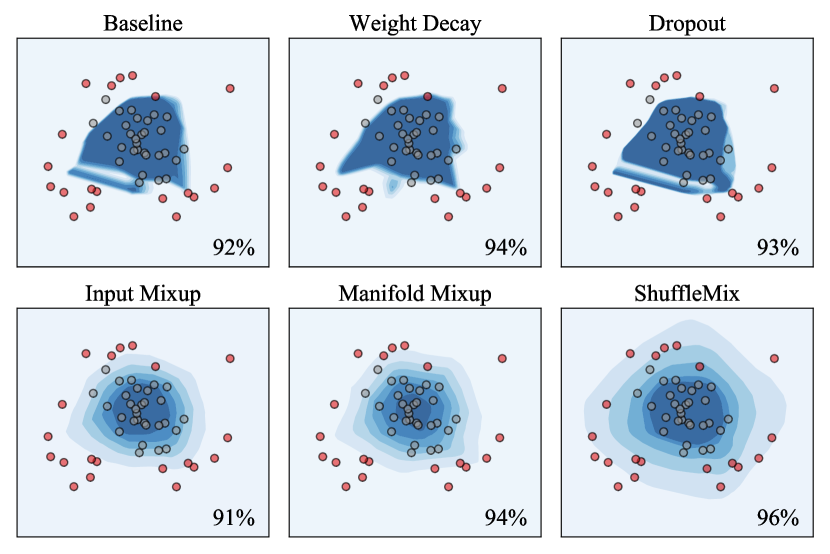
Figure 6: Decision boundaries for different methods on a synthetic dataset of binary classification, which is implemented with the scikit-learn [64] package. Classification accuracy of each method is presented in the bottom right of figure. (Best viewed in colors)

To illustrate advantages of our proposed ShuffleMix method, we further conduct binary classification experiments with several methods, i.e., the Weight Decay [32], the Dropout [13], the Mixup [10], and the Manifold Mixup [12], on a synthetic dataset, which is generated with the function of make circles in scikit-learn [64]. We use a neural network with four fully-connected (FC) layers and three ReLu modules as our Baseline. The Dropout with dropping rate of 0.2 is just applied to the final FC layer, while the weight decay is set as $5\times 10^{-4}$ just for the Weight Decay method. The hyper parameters in Input Mixup, Manifold Mixup, and our ShuffleMix are set the same as stated in Sec. V-A. Meanwhile, we conduct more experiments with the same hyper-parameters on a 3-classes synthetic dataset, for illustrating main differences among Input Mixup [10], Manifold Mixup [12], and our ShuffleMix on representation manifolds (c.f. Fig. 1(d)).

Visualization for binary classification is illustrated in Fig. 6, where we see that mixup style data augmentation methods can always obtain smoother decision boundaries of image classification than typical regularization methods, e.g., Weight Decay and Dropout. Meanwhile, our ShuffleMix can further obtain the better representation manifolds (ratio of samples falling into the darkest region) than the Mixup and the Manifold Mixup, owing to the more flexibility of our ShuffleMix.

VI Conclusion

In this paper, we propose a novel ShuffleMix feature augmentation method for supervised classification, which is designed in a generalized linear combination of high-level hidden representations. Such a simple yet effective design can improve model generalization owing to its soft dropout-like characteristics and robustness against input noises and data sparsity. The proposed ShuffleMix is verified its effectiveness not only for single-label image classification but also for multi-label image classification. Moreover, superior performance can further be achieved by combining the ShuffleMix with the noise injection. Extensive experiments on several popular datasets with multiple backbone networks can demonstrate consistently superior performance of our method to recent mixup-style data augmentation methods including the state-of-the-art methods.

References

- [1] J. Deng, W. Dong, R. Socher, L.-J. Li, K. Li, and L. Fei-Fei, “Imagenet: A large-scale hierarchical image database,” in Proceedings of the IEEE conference on computer vision and pattern recognition, 2009, pp. 248–255.
- [2] A. Krizhevsky, I. Sutskever, and G. E. Hinton, “Imagenet classification with deep convolutional neural networks,” Advances in Neural Information Processing Systems, vol. 25, 2012.
- [3] C. Szegedy, V. Vanhoucke, S. Ioffe, J. Shlens, and Z. Wojna, “Rethinking the inception architecture for computer vision,” in Proceedings of the IEEE conference on computer vision and pattern recognition, 2016, pp. 2818–2826.
- [4] K. He, X. Zhang, S. Ren, and J. Sun, “Deep residual learning for image recognition,” in Proceedings of the IEEE conference on computer vision and pattern recognition, 2016, pp. 770–778.
- [5] J. Zhang, Q. Wu, C. Shen, J. Zhang, and J. Lu, “Multilabel image classification with regional latent semantic dependencies,” IEEE Transactions on Multimedia, vol. 20, pp. 2801–2813, 2018.
- [6] Z.-M. Chen, X.-S. Wei, P. Wang, and Y. Guo, “Multi-label image recognition with graph convolutional networks,” in Proceedings of the IEEE/CVF Conference on Computer Vision and Pattern Recognition, 2019, pp. 5177–5186.
- [7] N. Lei, D. An, Y. Guo, K. Su, S. Liu, Z. Luo, S.-T. Yau, and X. Gu, “A geometric understanding of deep learning,” Engineering, vol. 6, no. 3, pp. 361–374, 2020.
- [8] N. Lei, K. Su, L. Cui, S.-T. Yau, and X. D. Gu, “A geometric view of optimal transportation and generative model,” Computer Aided Geometric Design, vol. 68, pp. 1–21, 2019.
- [9] M. Dai, H. Hang, and X. Guo, “Implicit data augmentation using feature interpolation for diversified low-shot image generation,” arXiv preprint arXiv:2112.02450, 2021.
- [10] H. Zhang, M. Cisse, Y. N. Dauphin, and D. Lopez-Paz, “mixup: Beyond empirical risk minimization,” International Conference on Learning Representations, 2018.
- [11] H. Guo, Y. Mao, and R. Zhang, “Mixup as locally linear out-of-manifold regularization,” in Proceedings of the AAAI Conference on Artificial Intelligence, vol. 33, no. 01, 2019, pp. 3714–3722.
- [12] V. Verma, A. Lamb, C. Beckham, A. Najafi, I. Mitliagkas, D. Lopez-Paz, and Y. Bengio, “Manifold mixup: Better representations by interpolating hidden states,” in International Conference on Machine Learning. PMLR, 2019, pp. 6438–6447.
- [13] N. Srivastava, G. Hinton, A. Krizhevsky, I. Sutskever, and R. Salakhutdinov, “Dropout: a simple way to prevent neural networks from overfitting,” The journal of machine learning research, vol. 15, no. 1, pp. 1929–1958, 2014.
- [14] J. Tompson, R. Goroshin, A. Jain, Y. LeCun, and C. Bregler, “Efficient object localization using convolutional networks,” in Proceedings of the IEEE conference on computer vision and pattern recognition, 2015, pp. 648–656.
- [15] G. Ghiasi, T.-Y. Lin, and Q. V. Le, “Dropblock: A regularization method for convolutional networks,” Advances in Neural Information Processing Systems, vol. 31, 2018.
- [16] C. Wei, S. Kakade, and T. Ma, “The implicit and explicit regularization effects of dropout,” in International Conference on Machine Learning. PMLR, 2020, pp. 10 181–10 192.
- [17] P. Mianjy, R. Arora, and R. Vidal, “On the implicit bias of dropout,” in International Conference on Machine Learning. PMLR, 2018, pp. 3540–3548.
- [18] L. Wu, J. Li, Y. Wang, Q. Meng, T. Qin, W. Chen, M. Zhang, T.-Y. Liu et al., “R-drop: regularized dropout for neural networks,” Advances in Neural Information Processing Systems, vol. 34, 2021.
- [19] X. Bouthillier, K. Konda, P. Vincent, and R. Memisevic, “Dropout as data augmentation,” arXiv preprint arXiv:1506.08700, 2015.
- [20] T. DeVries and G. W. Taylor, “Improved regularization of convolutional neural networks with cutout,” arXiv preprint arXiv:1708.04552, 2017.
- [21] S. Yun, D. Han, S. J. Oh, S. Chun, J. Choe, and Y. Yoo, “Cutmix: Regularization strategy to train strong classifiers with localizable features,” in Proceedings of the IEEE/CVF International Conference on Computer Vision, 2019, pp. 6023–6032.
- [22] Z. Zhong, L. Zheng, G. Kang, S. Li, and Y. Yang, “Random erasing data augmentation,” in Proceedings of the AAAI conference on artificial intelligence, vol. 34, no. 07, 2020, pp. 13 001–13 008.
- [23] X. Zhang, X. Zhou, M. Lin, and J. Sun, “Shufflenet: An extremely efficient convolutional neural network for mobile devices,” in Proceedings of the IEEE conference on computer vision and pattern recognition, 2018, pp. 6848–6856.
- [24] S. H. Lim, N. B. Erichson, F. Utrera, W. Xu, and M. W. Mahoney, “Noisy feature mixup,” in International Conference on Learning Representations, 2022. [Online]. Available: https://openreview.net/forum?id=vJb4I2ANmy
- [25] Y. Tokozume, Y. Ushiku, and T. Harada, “Between-class learning for image classification,” in Proceedings of the IEEE Conference on Computer Vision and Pattern Recognition, 2018, pp. 5486–5494.
- [26] J.-H. Lee, M. Z. Zaheer, M. Astrid, and S.-I. Lee, “Smoothmix: A simple yet effective data augmentation to train robust classifiers,” in Proceedings of the IEEE/CVF Conference on Computer Vision and Pattern Recognition Workshops, 2020, pp. 756–757.
- [27] J.-H. Kim, W. Choo, and H. O. Song, “Puzzle mix: Exploiting saliency and local statistics for optimal mixup,” in International Conference on Machine Learning. PMLR, 2020, pp. 5275–5285.
- [28] A. S. Uddin, M. S. Monira, W. Shin, T. Chung, and S.-H. Bae, “Saliencymix: A saliency guided data augmentation strategy for better regularization,” in International Conference on Learning Representations, 2020.
- [29] S. Huang, X. Wang, and D. Tao, “Snapmix: Semantically proportional mixing for augmenting fine-grained data,” in Proceedings of the AAAI Conference on Artificial Intelligence, vol. 35, no. 2, 2021, pp. 1628–1636.
- [30] S. Venkataramanan, Y. Avrithis, E. Kijak, and L. Amsaleg, “Alignmix: Improving representation by interpolating aligned features,” arXiv preprint arXiv:2103.15375, 2021.
- [31] C. Xu, J. Yang, H. Tang, H. Zou, C. Lu, and T. Zhang, “Shuffle augmentation of features from unlabeled data for unsupervised domain adaptation,” arXiv preprint arXiv:2201.11963, 2022.
- [32] I. Loshchilov and F. Hutter, “Decoupled weight decay regularization,” in International Conference on Learning Representations, 2018.
- [33] S. Ioffe and C. Szegedy, “Batch normalization: Accelerating deep network training by reducing internal covariate shift,” in International conference on machine learning. PMLR, 2015, pp. 448–456.
- [34] A. Hernández-García and P. König, “Data augmentation instead of explicit regularization,” arXiv preprint arXiv:1806.03852, 2018.
- [35] S. Hou and Z. Wang, “Weighted channel dropout for regularization of deep convolutional neural network,” in Proceedings of the AAAI Conference on Artificial Intelligence, vol. 33, no. 01, 2019, pp. 8425–8432.
- [36] L. Carratino, M. Cissé, R. Jenatton, and J.-P. Vert, “On mixup regularization,” arXiv preprint arXiv:2006.06049, 2020.
- [37] L. Zhang, Z. Deng, K. Kawaguchi, A. Ghorbani, and J. Zou, “How does mixup help with robustness and generalization?” in International Conference on Learning Representations, 2020.
- [38] S. Huang, Z. Xu, D. Tao, and Y. Zhang, “Part-stacked cnn for fine-grained visual categorization,” in Proceedings of the IEEE conference on computer vision and pattern recognition, 2016, pp. 1173–1182.
- [39] J. Fu, H. Zheng, and T. Mei, “Look closer to see better: Recurrent attention convolutional neural network for fine-grained image recognition,” in Proceedings of the IEEE conference on computer vision and pattern recognition, 2017, pp. 4438–4446.
- [40] H. Zheng, J. Fu, Z.-J. Zha, J. Luo, and T. Mei, “Learning rich part hierarchies with progressive attention networks for fine-grained image recognition,” IEEE Transactions on Image Processing, vol. 29, pp. 476–488, 2019.
- [41] R. Du, D. Chang, A. K. Bhunia, J. Xie, Z. Ma, Y.-Z. Song, and J. Guo, “Fine-grained visual classification via progressive multi-granularity training of jigsaw patches,” in European Conference on Computer Vision. Springer, 2020, pp. 153–168.
- [42] D. Chang, Y. Ding, J. Xie, A. Bhunia, X. Li, Z. Ma, M. Wu, J. Guo, and Y.-Z. Song, “The devil is in the channels: Mutual-channel loss for fine-grained image classification,” IEEE Transactions on Image Processing, vol. 29, pp. 4683–4695, 2020.
- [43] W. Shi, Y. Gong, X. Tao, D. Cheng, and N. Zheng, “Fine-grained image classification using modified dcnns trained by cascaded softmax and generalized large-margin losses,” IEEE Transactions on Neural Networks and Learning Systems, vol. 30, pp. 683–694, 2019.
- [44] Y. Ding, Z. Ma, S. Wen, J. Xie, D. Chang, Z. Si, M. Wu, and H. Ling, “Ap-cnn: Weakly supervised attention pyramid convolutional neural network for fine-grained visual classification,” IEEE Transactions on Image Processing, vol. 30, pp. 2826–2836, 2021.
- [45] M.-L. Zhang and Z.-H. Zhou, “A review on multi-label learning algorithms,” IEEE Transactions on Knowledge and Data Engineering, vol. 26, pp. 1819–1837, 2014.
- [46] W. Liu, X. Shen, H. Wang, and I. W.-H. Tsang, “The emerging trends of multi-label learning,” IEEE Transactions on Pattern Analysis and Machine Intelligence, vol. PP, 2021.
- [47] G. Huang, Z. Liu, L. Van Der Maaten, and K. Q. Weinberger, “Densely connected convolutional networks,” in Proceedings of the IEEE conference on computer vision and pattern recognition, 2017, pp. 4700–4708.
- [48] S. Yun, S. J. Oh, B. Heo, D. Han, J. Choe, and S. Chun, “Re-labeling imagenet: from single to multi-labels, from global to localized labels,” in Proceedings of the IEEE/CVF Conference on Computer Vision and Pattern Recognition, 2021, pp. 2340–2350.
- [49] T. Ridnik, E. Ben-Baruch, N. Zamir, A. Noy, I. Friedman, M. Protter, and L. Zelnik-Manor, “Asymmetric loss for multi-label classification,” in Proceedings of the IEEE/CVF International Conference on Computer Vision, 2021, pp. 82–91.
- [50] J. Wang, Y. Yang, J. Mao, Z. Huang, C. Huang, and W. Xu, “Cnn-rnn: A unified framework for multi-label image classification,” in Proceedings of the IEEE conference on computer vision and pattern recognition, 2016, pp. 2285–2294.
- [51] T. Chen, Z. Wang, G. Li, and L. Lin, “Recurrent attentional reinforcement learning for multi-label image recognition,” in Proceedings of the AAAI conference on artificial intelligence, vol. 32, no. 1, 2018.
- [52] F. Zhou, S. Huang, and Y. Xing, “Deep semantic dictionary learning for multi-label image classification,” in Proceedings of the AAAI Conference on Artificial Intelligence, vol. 35, no. 4, 2021, pp. 3572–3580.
- [53] S. Wen, W. Liu, Y. Yang, P. Zhou, Z. Guo, Z. Yan, Y. Chen, and T. Huang, “Multilabel image classification via feature/label co-projection,” IEEE Transactions on Systems, Man, and Cybernetics: Systems, vol. 51, no. 11, pp. 7250–7259, 2020.
- [54] Z. Wang, T. Chen, G. Li, R. Xu, and L. Lin, “Multi-label image recognition by recurrently discovering attentional regions,” in Proceedings of the IEEE international conference on computer vision, 2017, pp. 464–472.
- [55] A. Krizhevsky, “Learning multiple layers of features from tiny images,” Master’s thesis, Department of Computer Science, University of Toronto, 2009.
- [56] Y. Le and X. Yang, “Tiny imagenet visual recognition challenge,” CS 231N, vol. 7, no. 7, p. 3, 2015.
- [57] C. Wah, S. Branson, P. Welinder, P. Perona, and S. Belongie, “The caltech-ucsd birds-200-2011 dataset,” 2011.
- [58] J. Krause, M. Stark, J. Deng, and L. Fei-Fei, “3d object representations for fine-grained categorization,” in Proceedings of the IEEE international conference on computer vision workshops, 2013, pp. 554–561.
- [59] S. Maji, E. Rahtu, J. Kannala, M. Blaschko, and A. Vedaldi, “Fine-grained visual classification of aircraft,” arXiv preprint arXiv:1306.5151, 2013.
- [60] M. Everingham, L. V. Gool, C. K. I. Williams, J. M. Winn, and A. Zisserman, “The pascal visual object classes (voc) challenge,” International Journal of Computer Vision, vol. 88, pp. 303–338, 2009.
- [61] A. Paszke, S. Gross, F. Massa, A. Lerer, J. Bradbury, G. Chanan, T. Killeen, Z. Lin, N. Gimelshein, L. Antiga et al., “Pytorch: An imperative style, high-performance deep learning library,” Advances in Neural Information Processing Systems, vol. 32, 2019.
- [62] Y. Wei, W. Xia, M. Lin, J. Huang, B. Ni, J. Dong, Y. Zhao, and S. Yan, “Hcp: A flexible cnn framework for multi-label image classification,” IEEE Transactions on Pattern Analysis and Machine Intelligence, vol. 38, pp. 1901–1907, 2016.
- [63] M. Wang, C. Luo, R. Hong, J. Tang, and J. Feng, “Beyond object proposals: Random crop pooling for multi-label image recognition,” IEEE Transactions on Image Processing, vol. 25, pp. 5678–5688, 2016.
- [64] F. Pedregosa, G. Varoquaux, A. Gramfort, V. Michel, B. Thirion, O. Grisel, M. Blondel, P. Prettenhofer, R. Weiss, V. Dubourg, J. Vanderplas, A. Passos, D. Cournapeau, M. Brucher, M. Perrot, and E. Duchesnay, “Scikit-learn: Machine learning in Python,” Journal of Machine Learning Research, vol. 12, pp. 2825–2830, 2011.