History Repeats: Overcoming Catastrophic Forgetting For Event-Centric Temporal Knowledge Graph Completion

Abstract

Temporal knowledge graph (TKG) completion models typically rely on having access to the entire graph during training. However, in real-world scenarios, TKG data is often received incrementally as events unfold, leading to a dynamic non-stationary data distribution over time. While one could incorporate fine-tuning to existing methods to allow them to adapt to evolving TKG data, this can lead to forgetting previously learned patterns. Alternatively, retraining the model with the entire updated TKG can mitigate forgetting but is computationally burdensome. To address these challenges, we propose a general continual training framework that is applicable to any TKG completion method, and leverages two key ideas: (i) a temporal regularization that encourages repurposing of less important model parameters for learning new knowledge, and (ii) a clustering-based experience replay that reinforces the past knowledge by selectively preserving only a small portion of the past data. Our experimental results on widely used event-centric TKG datasets demonstrate the effectiveness of our proposed continual training framework in adapting to new events while reducing catastrophic forgetting. Further, we perform ablation studies to show the effectiveness of each component of our proposed framework. Finally, we investigate the relation between the memory dedicated to experience replay and the benefit gained from our clustering-based sampling strategy.

1 Introduction

Knowledge graphs (KGs) provide a powerful tool for studying the underlying structure of multi-relational data in the real world Liang et al. (2022). They present factual information in the form of triples, each consisting of a subject entity, a relation, and an object entity. Despite the development of advanced extraction techniques, knowledge graphs often suffer from incompleteness, which can lead to errors in downstream applications. As a result, the task of predicting missing facts in knowledge graphs, also known as knowledge graph completion, has become crucial. Wang et al. (2022); Huang et al. (2022); Shen et al. (2022)

KGs are commonly extracted from real-world data streams, such as newspaper texts that change and update over time, making them inherently dynamic. The stream of data that emerges every day may contain new entities, relations, or facts. As a result, facts in a knowledge graph are usually accompanied by time information. A fact in a semantic knowledge graph, such as Yago Kasneci et al. (2009), may be associated with a time interval, indicating when it appeared and remained in the KG. For example, consider (Obama, President, United States, 2009-2017) in a semantic KG. A link between Obama and United states appears in the graph after 2009, and it exists until 2017. On the other hand, a fact in a Temporal event-centric knowledge graph (TKGs), such as ICEWS Boschee et al. (2015), is associated with a single timestamp, indicating the exact time of the interaction between the subject and object entities. For example, in an event-centric TKG, (Obama, meet, Merkel) creates a link between Obama and Merkel several times within 2009 to 2017 since the temporal links only show the time when an event has occurred. Therefore, event-centric TKGs exhibit a high degree of dynamism and non-stationarity in contrast to semantic KGs.

To effectively capture the temporal dependencies within entities and relations in TKGs, as well as new patterns that may emerge with new data streams, it is necessary to develop models specifically designed for TKG completion. A significant amount of research has been dedicated to developing evolving models Messner et al. (2022); Mirtaheri et al. (2021); Jin et al. (2020); Garg et al. (2020) for TKG completion. These models typically assume evolving vector representations for entities or relations. These representations change depending on the timestep, and they can capture temporal dependencies between entities. However, these models often assume that the entire dataset is available during training. They do not provide a systematic method for updating model parameters when new data is added. One potential solution is to retrain the model with new data. However, this approach can be resource-intensive and impractical for large-scale knowledge graphs. An alternative approach is to fine-tune the model with new data, which is more time and memory efficient. However, this approach has been shown to be susceptible to overfitting to the new data, resulting in the model forgetting previously learned knowledge, a phenomenon known as catastrophic forgetting (Fig. 1). A limited number of studies Song and Park (2018); Daruna et al. (2021); Wu et al. (2021) have addressed this problem for semantic knowledge graphs using continual learning approaches, with TIE Wu et al. (2021) being the most closely related work to current research. Nevertheless, the development of efficient and effective methods for updating models with new data remains a significant challenge in event-centric Temporal Knowledge Graphs.

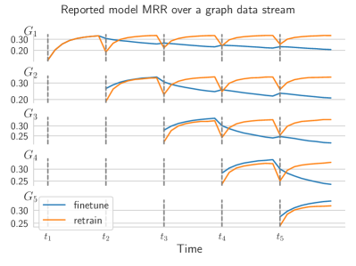
Figure 1: Catastrophic forgetting effect of fine-tuning. A TKG completion model is fine-tuned with the graph data at time $t_{i}$ and achieves the highest MRR score for $G_{i}$. The MRR scores decrease for $G_{1},...,G_{i-1}$.

We propose a framework for incrementally training a TKG completion model that consolidates the previously learned knowledge while capturing new patterns in the data. Our incremental learning framework employs regularization and experience replay to alleviate catastrophic forgetting. We propose a temporal regularization method based on elastic weight consolidation Kirkpatrick et al. (2017). By estimating an importance weight for every model parameter at each timestep, the regularization term in the objective function ’freezes’ the more important parameters from past timesteps, encouraging the use of less important parameters for learning the current task. Additionally, an exponentially decaying hyperparameter in the objective function further emphasizes the importance of the most recent tasks over older ones. Our selective experience replay method uses clustering over the representation of the data points to first capture the underlying structure of the data. The points closest to the clusters’ centroid are selected for experience replay. We show that the temporal regularization combined with clustering-based experience replay outperforms all the baselines in alleviating catastrophic forgetting. Our main contributions include:

1. A novel framework for incremental training and evaluation of event-centric TKGs, which addresses the challenges of efficiently updating models with new data.

2. A clustering-based experience replay method, which we show to be more effective than uniform sample selection. We also demonstrate that careful data selection for experience replay is crucial when memory is limited.

3. An augmentation of the training loss with a consolidation loss, specifically designed for TKG completion, which helps mitigate forgetting effects. We show that assigning a decayed importance to the older tasks reduces forgetting effects.

4. A thorough evaluation of the proposed methods through extensive quantitative experiments to demonstrate the effectiveness of our full training strategies compared to baselines.

2 Related Work

Our work is related to TKG completion, continual learning methods, and recent developments of continual learning for knowledge graphs.

2.1 Temporal Knowledge Graph Reasoning

TKG completion methods can be broadly categorized into two main categories based on their approach for encoding time information: translation-based methods and evolving methods.

Translation-based methods, such as those proposed by Leblay and Chekol (2018); García-Durán et al. (2018); Dasgupta et al. (2018); Wang and Li (2019); Jain et al. (2020), and Sadeghian et al. (2021), utilize a lower-dimensional space, such as a vector Leblay and Chekol (2018); Jain et al. (2020), or a hyperplane Dasgupta et al. (2018); Wang and Li (2019), for event timestamps and define a function to map an initial embedding to a time-aware embedding.

On the other hand, evolving models assume a dynamic representation for entities or relations that is updated over time. These dynamics can be captured by shallow encoders Xu et al. (2019); Mirtaheri et al. (2019); Han et al. (2020a) or sequential neural networks Trivedi et al. (2017); Jin et al. (2020); Wu et al. (2020); Zhu et al. (2020); Han et al. (2020b, c); Li et al. (2021). For example,Xu et al. (2019) model entities and relations as time series, decomposing them into three components using adaptive time series decomposition. DyERNIE Han et al. (2020a) propose a non-Euclidean embedding approach in the hyperbolic space. Trivedi et al. (2017) represent events as point processes, while  Jin et al. (2020) utilizes a recurrent architecture to aggregate the entity neighborhood from past timestamps.

2.2 Continual Learning

Continual learning (CL) or lifelong learning is a learning setting where a set of tasks are learned in a sequence. The major challenge in CL is overcoming catastrophic forgetting, where the model’s performance on past learned tasks is degraded as it is updated to learn new tasks in the sequence. Experience replay Li and Hoiem (2018) is a major approach to mitigate forgetting, where representative samples of past tasks are replayed when updating a model to retain past learned knowledge. To maintain a memory buffer storage with a fixed size, representative samples must be selected and discarded. Schaul et al. (2016) propose selecting samples that led to the maximum effect on the loss function when learning past tasks.

To relax the need for a memory buffer, generative models can be used to learn generating pseudo-samples. Shin et al. (2017) use adversarial learning for this purpose. An alternative approach is to use data generation using autoencodersRostami et al. (2020); Rostami and Galstyan (2023a). Weight consolidation is another important approach to mitigate catastrophic forgetting Zenke et al. (2017); Kirkpatrick et al. (2017). The idea is to identify important weights that play an important role in encoding the learned knowledge about past tasks and consolidate them when the model is updated to learn new tasks. As a result, new tasks are learned using primarily the free learnable weights. In our framework, we combine both approaches to achieve optimal performance.

2.3 Continual Learning for Graphs

CL in the context of graph structures remains an under-explored area, with a limited number of recent studies addressing the challenge of dynamic heterogeneous networks Tang and Matteson (2021); Wang et al. (2020); Zhou and Cao (2021) and semantic knowledge graphs Song and Park (2018); Daruna et al. (2021); Wu et al. (2021). In particular, Song and Park (2018); Daruna et al. (2021) propose methods that integrate class incremental learning models with static translation-based approaches, such as TransE Bordes et al. (2013), for addressing the problem of continual KG embeddings. Additionally, TIE Wu et al. (2021) develops a framework that predominantly focuses on semantic KGs, and generates yearly graph snapshots by converting a fact with a time interval into multiple timestamped facts. This process can cause a loss of more detailed temporal information, such as the month and date, and results in a substantial overlap of over 95% between consecutive snapshots. TIE’s frequency-based experience replay mechanism operates by sampling a fixed set of data points from a fixed-length window of past graph snapshots; for instance, at a given time $t$, it has access to the snapshots from $t-1$ to $t-5$. This contrasts with the standard continual learning practice, which involves sampling data points from the current dataset and storing them in a continuously updated, fixed-size memory buffer. When compared to Elastic Weight Consolidation (EWC), the L2 regularizer used by TIE proves to be more rigid when learning new tasks over time. Furthermore, their method’s evaluation is confined to shallow KG completion models like Diachronic Embeddings Goel et al. (2020) and HyTE Dasgupta et al. (2018).

3 Problem Definition

This section presents the formal definition of continual temporal knowledge graph completion.

3.1 Temporal Knowledge Graph Reasoning

A TKG is a collection of events represented as a set of quadruples $G=\{(s,r,o,\tau)|s,o\in\mathcal{E},r\in\mathcal{R}\}$, where $\mathcal{E}$ and $\mathcal{R}$ are the set of entities and relations, and $\tau$ is the timestamp of the event occurrence. These events represent one-time interactions between entities at a specific time. The task of temporal knowledge graph completion is to predict whether there will be an interaction between two entities at a given time. This can be done by either predicting the object entity, given the subject and relation at a certain time, or by predicting the relation between entities, given the subject and object at a certain time. In this case, we will focus on the first method which can be formally defined as a ranking problem. The model will assign higher likelihood to valid entities and rank them higher than the rest of the candidate entities.

3.2 Continual Learning Framework For Tempporal Knolwedge Graphs

A Temporal knowledge graph $G$ can be represented as a stream of graph snapshots $G_{1},G_{2},\dots,G_{T}$ arriving over time, where $G_{t}=\{(s,r,o,\tau)|s,o\in\mathcal{E},r\in\mathcal{R},\tau\in\left[\tau_{t},\tau_{t+1}\right)\}$ is a set of events occurred within time interval $\left[\tau_{t},\tau_{t+1}\right)$.

The continual training of a TKG completion method involves updating the parameters of the model $\mathcal{M}$ as new graph snapshots, consisting of a set of events, become available over time. This process aims to consolidate previously acquired information while incorporating new patterns. Formally, we define a set of tasks $\langle\mathcal{T}_{1},\dots,\mathcal{T}_{T}\rangle$, where each task $\mathcal{T}_{t}=\left(D_{t}^{train},D_{t}^{test},D_{t}^{val}\right)$ is comprised of disjoint subsets of the $G_{t}$ events, created through random splitting. A continually trained model $\mathcal{M}$ can then be shown as a stream of models $\mathcal{M}=\langle\mathcal{M}_{1},\dots,\mathcal{M}_{T}\rangle$, with corresponding parameter sets $\theta=\langle\theta_{1},\theta_{2},...,\theta_{T}\rangle$, trained incrementally as a stream of tasks arrive $\mathcal{T}=\langle\mathcal{T}_{1},\mathcal{T}_{2},...,\mathcal{T}_{T}\rangle$.

3.3 Base Model

In this paper, we utilize RE-Net Jin et al. (2020), a state-of-the-art TKG completion method, as the base model. RE-Net is a recurrent architecture for predicting future interactions, which models the probability of an event occurrence based on temporal sequences of past knowledge graphs. The model incorporates a recurrent event encoder to process past events and a neighborhood aggregator to model connections at the same time stamp. Although RE-Net was initially developed for predicting future events (extrapolation), it can also be used to predict missing links in the current state of the graph (interpolation), which is the focus of this study. The model parameterizes the probability of an event $p(\mathrm{o}_{\tau}|\mathrm{s},\mathrm{r})$ as follows:

$$p(\mathrm{o}_{\tau}|\mathrm{s},\mathrm{r})\propto\exp\left([\boldsymbol{e}_{\mathrm{s}}:\boldsymbol{e}_{\mathrm{r}}:\boldsymbol{h}_{\tau-1}(\mathrm{s},\mathrm{r})]^{\top}\cdot\boldsymbol{w}_{\mathrm{o}_{\tau}}\right),$$ (1)

where $\boldsymbol{e}_{\mathrm{s}},\boldsymbol{e}_{\mathrm{r}}\in\mathbb{R}^{d}$ are learnable embedding vectors for the subject entity $\mathrm{s}$ and relation $\mathrm{r}$. $\boldsymbol{h}_{\tau-1}(\mathrm{s},\mathrm{r})\in\mathbb{R}^{d}$ represents the local dynamics within a time window $(\tau-\ell,\tau-1)$ for $(\mathrm{s},\mathrm{r})$. By combining both the static and dynamic representations, RE-Net effectively captures the semantics of $(\mathrm{s},\mathrm{r})$ up to time stamp $(\tau-1)$. The model then calculates the probability of different object entities $\mathrm{o}_{\tau}$ by passing the encoding through a multi-layer perceptron (MLP) decoder, which is defined as a linear softmax classifier parameterized by ${\boldsymbol{w}_{\mathrm{o}_{\tau}}}$.

4 Methodology

Our proposed framework is a training approach that can be applied to any TKG completion model. It enables the incremental updating of model parameters with new data while addressing the issues of catastrophic forgetting associated with fine-tuning. To achieve this, we utilize experience replay and regularization techniques - methodologies commonly employed in image processing and reinforcement learning to mitigate forgetting. Additionally, we introduce a novel experience replay approach that employs clustering to identify and select data points that best capture the underlying structure of the data. Furthermore, we adopt the regularization method of EWC, as proposed in [Kirkpatrick et al., 2017], which incorporates a decay parameter that assigns higher priority to more recent tasks. Our results demonstrate that the incorporation of a decay parameter into the EWC loss and prioritizing more recent tasks leads to improved performance.

4.1 Experience Replay

In the field of neuroscience, the hippocampal replay, or the re-activation of specific trajectories, is a crucial mechanism for various neurological functions, including memory consolidation. Motivated by this concept, the use of experience replay in Continual Learning (CL) for deep neural networks aims to consolidate previously learned knowledge when a new task is encountered by replaying previous experiences, or training the model on a limited subset of previous data points. However, a challenge with experience replay, also known as memory-based methods, is the requirement for a large memory size to fully consolidate previous tasks Rostami and Galstyan (2023b). Thus, careful selection of data points that effectively represent the distribution of previous data becomes necessary.

In this work, we propose the use of experience replay for continual TKG completion. Specifically, we maintain a memory buffer $\mathcal{B}$ which, at time $t$, contains a subset of events sampled from $D^{train}_{1},D^{train}_{2},\dots,D^{train}_{t-1}$. When Task $\mathcal{T}_{t}$ is presented to the model, it is trained on the data points in $D^{train}_{t}\cup\mathcal{B}$. After training, a random subset of events in the memory buffer, $\frac{|\mathcal{B}|}{t}$, are discarded and replaced with a new subset of events sampled from $D^{train}_{t}$. In this way, at time $t$, where $t$ tasks have been observed, equal portions of memory with size $\frac{|\mathcal{B}|}{t}$ are dedicated to each task. A naive approach for selecting a subset of events from a task’s training set at time $t$ would be to uniformly sample $\frac{|\mathcal{B}|}{t}$ events from $D^{train}_{t}$. However, we propose a clustering-based sampling method that offers a more careful selection algorithm, which is detailed in the following section.

4.1.1 Clustering-based Sampling

When dealing with complex data, it is likely that various subspaces exist within the data that must be represented in the memory buffer. To address this issue, clustering methods are employed to diversify the memory buffer by grouping data points into distinct clusters. The centroids of these clusters can be utilized as instances themselves or as representatives of parts of the memory buffer.Shi et al. (2018); Hayes et al. (2019); Korycki and Krawczyk (2021). In this study, clustering is applied to the representation of events in the training set in order to uncover the underlying structure of the data and select data points that effectively cover the data distribution. The Hierarchical Density-Based Spatial Clustering of Applications with Noise (HDBSCAN) algorithm McInnes et al. (2017) is utilized for this purpose. HDBSCAN is a hierarchical, non-parametric, density-based clustering method that groups points that are closely packed together while identifying points in low-density regions as outliers.

The use of HDBSCAN over other clustering methods is advantageous due to its minimal requirements for hyperparameters. Many clustering algorithms necessitate and are sensitive to the number of clusters as a hyperparameter. However, HDBSCAN can determine the appropriate number of clusters by identifying and merging dense space regions. Additionally, many clustering algorithms are limited to finding only spherical clusters. HDBSCAN, on the other hand, is capable of uncovering more complex underlying structures in the data. As a result of its ability to identify clusters with off-shaped structures, HDBSCAN generates a set of exemplar points for each cluster rather than a single point as the cluster centroid.

We represent each event $(s,r,o,\tau)\in D^{train}_{t}$ as a vector $[\boldsymbol{e}_{\mathrm{s}}:\boldsymbol{e}_{\mathrm{o}}]\in\mathbb{R}^{2d}$, where $\boldsymbol{e}_{\mathrm{s}}$ and $\boldsymbol{e}_{\mathrm{o}}$ represent the $d$-dimensional embeddings of $s$ and $o$ at time $t$, respectively. The notation [:] denotes concatenation, creating a $|D^{train}_{t}|\times 2d$ matrix that represents the training data at time $t$. In our initial experiments, we found that data representations such as $[\boldsymbol{e}_{\mathrm{s}}:\boldsymbol{e}_{\mathrm{r}}]$, where $\boldsymbol{e}_{\mathrm{r}}$ is the relation embeddings, did not significantly affect the results. Moreover, representing the data as $[\boldsymbol{e}_{\mathrm{s}}:\boldsymbol{e}_{\mathrm{r}}:\boldsymbol{e}_{\mathrm{o}}]$ led to a bias towards relation representation, causing data points with identical relation types to cluster together.

We obtained clusters $\mathcal{C}^{1},\mathcal{C}^{2},\dots,\mathcal{C}^{m}$ by running HDBSCAN. Our algorithm then selects $\frac{|\mathcal{B}|}{t}$ events from these clusters by prioritizing the data points closest to the exemplars and giving precedence to larger clusters. If $\frac{|\mathcal{B}|}{t}<m$, data points are chosen only from the first $\frac{|\mathcal{B}|}{t}$ clusters. Conversely, if $\frac{|\mathcal{B}|}{t}>m$, the number of points selected from each cluster will depend on the cluster size, with a minimum of one data point chosen from each cluster. The specifics of this procedure are detailed further in Algorithm 1.

input: $\mathcal{C}_{t}=\mathcal{C}^{1}_{t},\mathcal{C}^{2}_{t},\dots,\mathcal{C}^{m}_{t}$ (clusters generated with hdbscan from $D^{train}_{t}$ sorted in decreasing order of their size; $D^{train}_{t}$ (training set at time $t$); $s$ (sample size); $\textsc{{FindExemplars}}(\mathcal{C}^{i},k)$ (Takes a cluster and returns $k$ points closests to the cluster exemplars.)

1 def SelectPoints($\mathcal{C}_{t}$, $D^{train}_{t}$, $s$):

      2 $Q\leftarrow\emptyset$

      3 for $i\leftarrow 1$ to $m$  do

            4 $r\leftarrow\lceil\frac{|\mathcal{C}^{i}|}{\sum_{j}|\mathcal{C}^{j}|}\times s\rceil$

            5 $\mathcal{X}\leftarrow\textsc{{FindExemplars}}(\mathcal{C}^{i},r)$

            6 $Q\leftarrow Q\cup(\mathcal{X},r)$

      7$S\leftarrow\emptyset$

      8 while $Q\neq\emptyset\And|S|<s$ do

            9 $\mathcal{X},r\leftarrow Q.\texttt{pop}()$

            10 $S\leftarrow S\cup[\mathcal{X}[0]]$

            11 $Q\leftarrow Q\cup(\mathcal{X}[1:],r-1)$

      12return $S$

Algorithm 1 Cluster Experience Replay

4.2 Regularization

Regularization-based approaches for CL incorporate a regularization term in the objective function to discourage changes in the weights that are crucial for previous tasks, while encouraging the utilization of other weights. One such approach, Elastic Weight Consolidation (EWC) Kirkpatrick et al. (2017), estimates the importance of weights using the Fisher Information Matrix. Given a model with parameter set $\theta$ previously trained on task $A$, and a new task B, EWC optimizes the following loss function:

$$\mathcal{L}(\theta)=\mathcal{L}_{B}(\theta)+\sum_{i}\frac{\lambda}{2}F_{i}(\theta_{i}-\theta^{*}_{A,i})^{2}$$ (2)

Where $\mathcal{L}_{B}$ is the loss over task $B$ only and $\lambda$ determines the importance of the previous task compared to task $B$. We extend this loss function for continual TKG completion. Given a stream of tasks $\langle\mathcal{T}_{1},\mathcal{T}_{2}\dots,\mathcal{T}_{t}\rangle$ and incrementally obtained parameter sets $\langle\theta_{1},\theta_{2}\dots,\theta_{t}\rangle$, we define the temporal EWC loss functions as follows:

$$\mathcal{L}(\theta_{t})=\mathcal{L}_{\mathcal{T}_{t}}(\theta_{t})+\sum_{\tau=1}^{t-1}\sum_{i}\frac{\lambda}{2}F_{\tau}(\theta_{i}-\theta^{*}_{\tau,i})^{2}$$ (3)

Where $\mathcal{L}_{\mathcal{T}_{t}}$ is the model loss calculated only using $\mathcal{M}_{t}$ and $D^{train}_{t}$, $F_{\tau}$ is the Fisher Information Matrix estimated for $\mathcal{M}_{\tau}$ and $\mathcal{T}_{\tau}$ and $\theta_{\tau,i}$ is $i$-th parameter of $\mathcal{M}_{\tau}$. The $\lambda$ parameter in Equation 3 assigns equal importance to all the tasks from previous time steps, however, in practice, and depending on the application, different tasks might have different effect on the current task making plausibility of adaptive $\lambda_{\tau}$:

$$\mathcal{L}(\theta_{t})=\mathcal{L}_{\mathcal{T}_{t}}(\theta_{t})+\sum_{\tau=1}^{t-1}\sum_{i}\frac{\lambda_{\tau}}{2}F_{\tau}(\theta_{i}-\theta^{*}_{\tau,i})^{2},$$ (4)

where $\lambda_{\tau}=\lambda\alpha^{t-\tau}$, $\lambda$ is the overall EWC loss importance, and $\alpha<1$ is the decay parameter.

4.3 Training and Loss Function

The final loss function of our framework, when trained with experience replay and EWC can be summarized as follows:

$$\begin{split}&\mathcal{L}(\theta_{t})=\mathcal{L}_{expr}(\theta_{t})+\lambda\mathcal{L}_{ewc}(\theta_{t}),\\ &\mathcal{L}_{expr}(\theta_{t})=\mathcal{L}_{\mathcal{T}_{t}\cup\mathcal{B}}(\theta_{t}),\\ &\mathcal{L}_{ewc}=\sum_{\tau=1}^{t-1}\sum_{i}\frac{\alpha^{t-\tau}}{2}F_{\tau}(\theta_{i}-\theta^{*}_{\tau,i})^{2}\end{split}$$ (5)

The replay loss $\mathcal{L}_{expr}$ is the model loss trained over both the current task’s training set $D^{train}_{t}$ and the data points in the memory buffer $\mathcal{B}$. For training in batches, the number of data points selected from $D^{train}_{t}$ and $\mathcal{B}$ is in proportion to their size.

5 Experiments

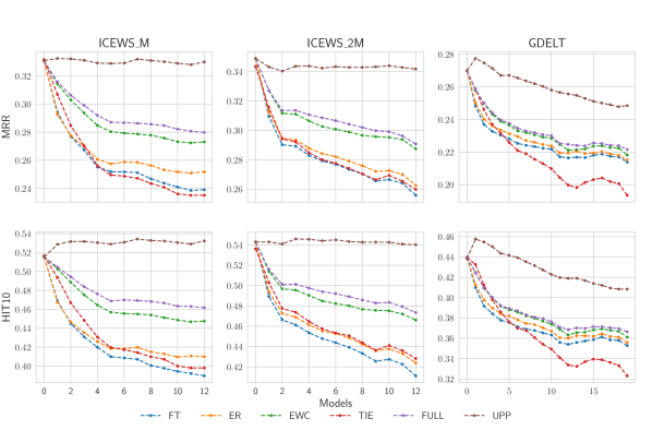
Figure 2: The overall performance comparison. Average Hit@10 and average MRR reported for RE-Net incrementally trained using three benchmarks: ICEWS-M, ICEWS-2M, and GDELT.

In this section, we explain the evaluation protocol to quantitatively measuring the model catastrophic forgetting. From know TKG datasets, we create two benchmarks for TKG continual learning. We evaluate our proposed training method using the benchmark, compare them with various baselines and show the effectiveness of our approach in alleviating catastrophic forgetting. Finally, we conduct ablation studies on different components of our training method to validate our model.

5.1 Datasets

Dataset	#tasks	task period	split ratio	avg #quads train/test
ICEWS-M	13	1 month	50/25/25	27k/13k
ICEWS-2M	13	2 month	50/25/25	50k/25k
GDELT	21	3 days	60/20/20	38k/13k

Table 1: Dataset statistics

We use two datasets: the Integrated Crisis Early Warning System (ICEWS) and the Global Database of Events, Language, and Tone (GDELT). Both datasets contain interactions between geopolitical actors, with daily event dates in the ICEWS dataset and 15-minute intervals in the GDELT dataset. To create benchmarks, we use a one-year period of the ICEWS dataset starting from 01-01-2015 and consider each month as a separate graph snapshot (ICEWS-M). We also use a two-year period from 01-01-2015 to 02-01-2017, dividing it into 13 graph snapshots with 2-month windows (ICEWS-2M). We split the events in each snapshot into train, validation, and test sets with a 50/25/25 percent ratio. For the GDELT, we use a 20-day period, dividing it into 3-day windows and split the data into train/test/validation sets with a 60/20/20 percent ratio. Table 1 includes statistics for each benchmark. We assume that all relations and entities are known at all times during training, and no new entities or relations are presented to the model.

5.2 Evaluation Setup

We start by training $\mathcal{M}$ over $D^{train}_{1}$ and use $D^{val}_{1}$ for hyper-parameter tuning. The model $\mathcal{M}_{t}$ with parameter set $\theta_{t}$ at time step $t$ is first initialized with parameters from the previous time step $\theta_{t-1}$. Then $\mathcal{M}_{t}$ parameters are updated by training the model over $D^{train}_{t}$. The training step can be a simple fine-tuning, or it can be augmented with data points for experience replay or with the temporal EWC loss.

In order to assess the forgetting effect, at time $t$, we report the average $\mathcal{M}_{t}$ performance over the current and all the previous test sets $D^{test}_{1},D^{test}_{2},\dots,D^{test}_{t}$. Precisely, we report the performance at time $t$ as $P_{t}=\frac{1}{t}\sum_{j=1}^{t}p_{t,j}$, where $p_{t,j}$ is the performance of $\mathcal{M}_{t}$ measured by either MRR or Hit@10 over $D^{test}_{j}$.

5.3 Comparative Study

To evaluate the performance of our incremental training framework, we conduct a comparative analysis with several baseline strategies. These include:

• FT: This strategy fine-tunes the model using the original loss function and the newly added data points.

• ER: This method applies experience replay Rolnick et al. (2019) with randomly chosen points. It then fine-tunes the model with both newly added events and events stored in the memory buffer.

• EWC Kirkpatrick et al. (2017): In this strategy, the model is trained with a loss function augmented by an EWC (Elastic Weight Consolidation) loss, as defined in Equation 3.

• TIE Wu et al. (2021): Drawing from TIE’s methodology, we incorporated L2 regularization into our objective function and utilized their implementation of frequency-based experience replay.

• Full: Our comprehensive model is trained using a clustering-based experience replay mechanism, supplemented with a decayed EWC loss.

	ICEWS-M				ICEWS-2M				GDELT
	Current		Average		Current		Average		Current		Average
Model	H@10	MRR	H@10	MRR	H@10	MRR	H@10	MRR	H@10	MRR	H@10	MRR
FT	$.503$	$.325$	$.390\pm.04$	$.239\pm.03$	$.517$	$.330$	$.411\pm.04$	$.256\pm.03$	$.421$	$.260$	$.351\pm.02$	$.214\pm.02$
ER	$.491$	$.314$	$.410\pm.03$	$.252\pm.02$	$.521$	$.331$	$.424\pm.04$	$.263\pm.03$	$.429$	$.263$	$.356\pm.02$	$.215\pm.02$
EWC	$.483$	$.299$	$.448\pm.03$	$.273\pm.02$	$.475$	$.294$	$.466\pm.02$	$.288\pm.02$	$.429$	$.262$	$.359\pm.02$	$.217\pm.02$
TIE	$.548$	$.354$	$.398\pm.05$	$.235\pm.04$	$.567$	$.362$	$.428\pm.05$	$.260\pm.04$	$.492$	$.309$	$.322\pm.05$	$.192\pm.03$
OURS	$.565$	$.358$	$\mathbf{.462\pm.04}$	$\mathbf{.280\pm.03}$	$.555$	$.349$	$\mathbf{.473\pm.03}$	$\mathbf{.291\pm.02}$	$.416$	$.256$	$\mathbf{.365\pm.02}$	$\mathbf{.222\pm.01}$

Table 2: Performance comparison (Hit@10 and MRR) of the RE-NET model incrementally trained using three benchmarks: ICEWS-M, ICEWS-2M, and GDELT. Performance is evaluated at the final training time step over the last test dataset(Current) and across all prior test datasets (Average).

Additionally, we train an upper-bound model, denoted as UPP. During the $t$-th step of training, this model has access to all training data from all preceding time steps, $1,\dots,t$. Detailed information about hyperparameter selection and implementation is provided in Appendix A. The results of this experiment, summarized in Fig. 2, demonstrate that our full training framework outperforms all other incremental training strategies in alleviating catastrophic forgetting. The L2 regularization used with TIE proves to be overly restrictive, leading to an even greater performance drop than that observed with the finetuning strategy. Table 2 summarizes the performance of the model at the final training time step on the last test dataset (referred to as ’current’), as well as its average performance across all previous test datasets (referred to as ’average’). Despite a slight dip in performance on the current task, our method consistently delivers a higher average performance. This discrepancy underscores the trade-off inherent in our approach, which is deliberately calibrated to strike a balance between maintaining high performance across all tasks and mitigating the forgetting of prior tasks.

5.4 Ablation Study

In this section, we present an ablation study to evaluate the effectiveness of our proposed approach. Fig. 3 illustrates the results of various variations of our model, trained on ICEWS-M and evaluated using average MRR as the performance metric. The variations include: (1) Random Experience Replay (RER), where points are randomly sampled uniformly; (2) Clustering-based Experience Replay (CER), where points are sampled using the method described in Section 4.1.1; (3) Regular EWC outlined in Equation 3 (EWC); (4) Decayed Elastic Weight Consolidation (DEWC), using the decayed $\lambda$ value outlined in Equation 4; and (5) DEWC + CER, which represents our full model.

Our results demonstrate that the individual components of our model play a role in enhancing the overall performance, with clustering-based experience replay showing superior performance compared to random experience replay. Additionally, the decayed EWC technique proves to be more effective than the traditional EWC when tasks are assigned equal importance coefficients. For a more in-depth understanding, the detailed results for all datasets used in the ablation study are provided in the Appendix B.

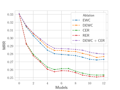
Figure 3: Ablation study on different components of the model using ICEWS-M. RER and CER stand for random and clustering-based experience replay. DEWC is the EWC with decayed $\lambda$ values.

5.5 EWC Variations

In order to demonstrate the effectiveness of the EWC loss with weight decay (as outlined in Equation 4), we are comparing it against three other variations of the EWC loss. We will train the RE-Net method incrementally, using each variation of the EWC loss separately. The results of this comparison can be seen in Fig. 4, which shows the average MRR score for a model trained incrementally with each loss variation, using the ICEWS-M dataset. The other variations of the EWC loss that we are comparing against include: (i) only using the parameters of the previous task for regularization, and only computing the Fisher Information Matrix for the previous task; (ii) using all previous task parameters for regularization, but giving all tasks the same importance coefficient value $\lambda$, and computing the Fisher Information Matrix for each task separately (as outlined in Equation 3); and (iii) a variation similar to the second one, but with the decayed $\lambda_{i}$ values of Equation 4 being assigned to each task randomly. The results in Fig. 4 indicate that using only the parameters of the previous task for regularization performs the worst. Using the same $\lambda$ value for all tasks has a smoothing effect on the Fisher Information Matrix, and this is why the decayed, permuted $\lambda$ values perform better. Our proposed loss ultimately outperforms all variations, highlighting the importance of more recent tasks compared to older tasks. As a potential next step, we could investigate learning $\lambda$ values based on task similarities.

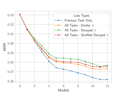
Figure 4: Comparison of EWC loss variations on model performance. Blue line represents using only the previous task in EWC loss, showing a significant reduction compared to considering all tasks.

5.6 Memory size and Experience Replay

This experiment compares the effectiveness of clustering-based sampling and uniform sampling for experience replay when memory is limited. We use ICEWS-M and run RE-Net with two types of experience replay: (i) random (uniform) sampling (RER) and (ii) clustering-based sampling (CER) using buffer sizes from 2000 to 11000 data points. We evaluated the model performance for $\mathcal{M}_{4}$, $\mathcal{M}_{8}$, and $\mathcal{M}_{12}$ which were trained incrementally with experience replay up to time 4, 8, and 12, respectively. We measure the performance of the model by taking the average MRR score over the first $4,8,12$ test sets for $\mathcal{M}_{4},\mathcal{M}_{8},\mathcal{M}_{12}$ respectively. Finally, we compare the performance of RER and CER methods by subtracting the RER model performance from the CER model performance, and the results are shown in Fig. 5. The results, shown in Fig. 5, indicate that when memory is very small or very large, there is no significant difference between RER and CER methods; when memory is too small, there is not enough information for the model to have a significant impact on performance, and when memory is too large, important data points are likely to be selected at random. However, when memory is sufficient, clustering-based sampling becomes more important.

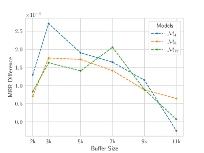
Figure 5: Comparison of average MRR for CER and RER. Results show no significant difference when memory is very small or large, but CER is more effective with sufficient memory.

6 Conclusion

We propose a framework for incrementally training a TKG completion model that consolidates the previously learned knowledge while capturing new patterns in the data. Our incremental learning framework employs regularization and experience replay techniques to alleviate the forgetting problem. Our regularization method is based on temporal elastic weight consolidation that assigns higher importance to the parameters of the more recent tasks. Our selective experience replay method uses clustering over the representation of the data points and selects the data points that best represent the underlying data structure. Our experimental results demonstrate the effectiveness of our proposed approach in alleviating the catastrophic forgetting for the event-centric temporal knowledge graphs. This work is the first step towards incremental learning for event-centric knowledge graphs. Potential future work might involve exploring, and taking into consideration the effect of time on task similarities which might differ for various applications.

7 Limitations

In this section, we examine the limitations of our approach. Even though our training methodology runs faster and uses less memory than retraining, there remains potential for further scalability optimization. One potential avenue for improvement could involve optimizing the estimation of the Fisher Information Matrix. Furthermore, optimizing the parameters related to the incremental training such as buffer size and regularization coefficient is dependent on the entire time steps rather than the current time steps. Devising a time-efficient way for hyperparameter optimization could be extremely beneficial for this task. Additionally, while our full model has demonstrated some mitigation of the problem of catastrophic forgetting, a significant gap remains between the upper performance bound and the performance of our approach. Further research is necessary to bridge this gap and improve overall performance. Finally, our current focus on continual learning is limited to the emergence of new events and does not currently consider the possibility of new relations or entities. This limitation is in part due to the base model (RE-Net) not being inductive and is a problem that is inherent to the model itself. Future research in the field of continual learning may aim to address this limitation by considering new relations and entities, even in the context of base models that do not support these features.

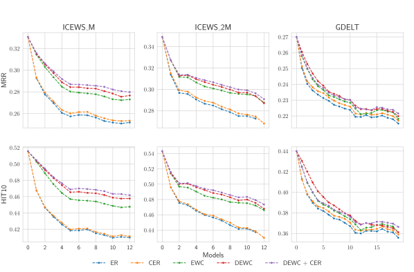
Figure 6: Ablation study on different components of the model using ICEWS-M, ICEWS-2M, and GDELT. RER and CER stand for random and clustering-based experience replay. DEWC is the EWC with decayed $\lambda$ values.

Appendix A Implementation Detail & Hyperparameters

We implemented our models using PyTorch, utilizing the RE-Net implementation from their GitHub repository as a base. We modified the training pipeline of RE-Net and added experience replay and regularization loss. The RE-Net model utilized a mean pooling layer for the neighborhood encoder, with a dropout of $0.5$ and an embedding dimension of $100$ for relations and entities. For the model variation that employed only EWC loss, we set the learning rate to $10^{-3}$. The regularization coefficient for EWC is set to $10$ and the weight decay to $0.9$ for all the datasets. For variations that included experience replay buffer or fine-tuning, we began training with a learning rate of $10^{-3}$ and decreased it to $10^{-4}$ for subsequent time steps. The buffer size was set to $3000$ for ICEWS-M and GDELT and $5000$ for ICEWS-2M, and the batch size was $256$ for ICEWS-M and GDELT and $512$ for ICEWS-2M. We selected the best model using the validation set at each time step. We ran each experiment once for each set of hyperparameters as the RE-Net performance did not vary significantly between runs. The min cluster size for HDBSCAN is set to 5 for all three datasets. We run all the experiments on machines with NVIDIA GeForce RTX 2080 Ti GPUs.

Appendix B Extended Ablation Study

In this section, we present the results of the ablation study conducted in Section 5.4 to evaluate the effectiveness of our method. Fig. 6 illustrates various variations of our model, which were trained incrementally over ICEWS-M, ICEWS-2M and GDELT using the hyperparameters reported in the previous section. The model variations include (1) Random Experience Replay (RER), where points are randomly sampled uniformly; (2) Clustering-based Experience Replay (CER), where points are sampled using the method described in Section 4.1.1; (3) Regular EWC outlined in Equation 3 (EWC); (4) Decayed Elastic Weight Consolidation (DEWC), using the decayed $\lambda$ value outlined in Equation 4; and (5) DEWC + CER, which represents our full model. The results indicate that clustering-based experience replay outperforms random experience replay, and that the DEWC approach is more effective for the ICEWS datasets compared to GDELT. This may be due to the fact that the data distribution for ICEWS datasets changes more significantly over the course of a year compared to GDELT, which only includes 21 days of data. It is also visible from the plots that the GDELT dataset exhibits less forgetting compared to both ICEWS datasets. Finally, the full model (DEWC + CER) always outperforms the other model variations, demonstrating the effectiveness of our methodology.

References

- Bordes et al. (2013) Antoine Bordes, Nicolas Usunier, Alberto Garcia-Duran, Jason Weston, and Oksana Yakhnenko. 2013. Translating embeddings for modeling multi-relational data. Advances in neural information processing systems, 26.
- Boschee et al. (2015) E Boschee, J Lautenschlager, S O’Brien, S Shellman, J Starz, and M Ward. 2015. Integrated crisis early warning system (icews) coded event data. URL: https://dataverse. harvard. edu/dataverse/icews.
- Daruna et al. (2021) Angel Daruna, Mehul Gupta, Mohan Sridharan, and Sonia Chernova. 2021. Continual learning of knowledge graph embeddings. IEEE Robotics and Automation Letters, 6:1128–1135.
- Dasgupta et al. (2018) Shib Sankar Dasgupta, Swayambhu Nath Ray, and Partha Talukdar. 2018. Hyte: Hyperplane-based temporally aware knowledge graph embedding. In Proceedings of EMNLP, pages 2001–2011.
- García-Durán et al. (2018) Alberto García-Durán, Sebastijan Dumančić, and Mathias Niepert. 2018. Learning sequence encoders for temporal knowledge graph completion. arXiv preprint arXiv:1809.03202.
- Garg et al. (2020) Sankalp Garg, Navodita Sharma, Woojeong Jin, and Xiang Ren. 2020. Temporal attribute prediction via joint modeling of multi-relational structure evolution. arXiv preprint arXiv:2003.03919.
- Goel et al. (2020) Rishab Goel, Seyed Mehran Kazemi, Marcus Brubaker, and Pascal Poupart. 2020. Diachronic embedding for temporal knowledge graph completion. In Proceedings of AAAI, volume 34, pages 3988–3995.
- Han et al. (2020a) Zhen Han, Peng Chen, Yunpu Ma, and Volker Tresp. 2020a. Dyernie: Dynamic evolution of riemannian manifold embeddings for temporal knowledge graph completion. arXiv preprint arXiv:2011.03984.
- Han et al. (2020b) Zhen Han, Peng Chen, Yunpu Ma, and Volker Tresp. 2020b. xerte: Explainable reasoning on temporal knowledge graphs for forecasting future links. arXiv preprint arXiv:2012.15537.
- Han et al. (2020c) Zhen Han, Yunpu Ma, Yuyi Wang, Stephan Günnemann, and Volker Tresp. 2020c. Graph hawkes neural network for forecasting on temporal knowledge graphs. In Automated Knowledge Base Construction.
- Hayes et al. (2019) Tyler L Hayes, Nathan D Cahill, and Christopher Kanan. 2019. Memory efficient experience replay for streaming learning. In 2019 International Conference on Robotics and Automation (ICRA), pages 9769–9776. IEEE.
- Huang et al. (2022) Zijie Huang, Zheng Li, Haoming Jiang, Tianyu Cao, Hanqing Lu, Bing Yin, Karthik Subbian, Yizhou Sun, and Wei Wang. 2022. Multilingual knowledge graph completion with self-supervised adaptive graph alignment. arXiv preprint arXiv:2203.14987.
- Jain et al. (2020) Prachi Jain, Sushant Rathi, Soumen Chakrabarti, et al. 2020. Temporal knowledge base completion: New algorithms and evaluation protocols. arXiv preprint arXiv:2005.05035.
- Jin et al. (2020) Woojeong Jin, Meng Qu, Xisen Jin, and Xiang Ren. 2020. Recurrent event network: Autoregressive structure inference over temporal knowledge graphs. In Proceedings of EMNLP, pages 6669–6683.
- Kasneci et al. (2009) Gjergji Kasneci, Maya Ramanath, Fabian Suchanek, and Gerhard Weikum. 2009. The yago-naga approach to knowledge discovery. ACM SIGMOD Record, 37(4):41–47.
- Kirkpatrick et al. (2017) James Kirkpatrick, Razvan Pascanu, Neil Rabinowitz, Joel Veness, Guillaume Desjardins, Andrei A Rusu, Kieran Milan, John Quan, Tiago Ramalho, Agnieszka Grabska-Barwinska, et al. 2017. Overcoming catastrophic forgetting in neural networks. Proceedings of the national academy of sciences, 114(13):3521–3526.
- Korycki and Krawczyk (2021) Lukasz Korycki and Bartosz Krawczyk. 2021. Class-incremental experience replay for continual learning under concept drift. In Proceedings of the IEEE/CVF Conference on Computer Vision and Pattern Recognition, pages 3649–3658.
- Leblay and Chekol (2018) Julien Leblay and Melisachew Wudage Chekol. 2018. Deriving validity time in knowledge graph. In Companion Proc. of the The Web Conference, pages 1771–1776.
- Li and Hoiem (2018) Zhizhong Li and Derek Hoiem. 2018. Learning without forgetting. IEEE Transactions on Pattern Analysis and Machine Intelligence, 40(12):2935–2947.
- Li et al. (2021) Zixuan Li, Xiaolong Jin, Wei Li, Saiping Guan, Jiafeng Guo, Huawei Shen, Yuanzhuo Wang, and Xueqi Cheng. 2021. Virtual event, canada 1,2. 2021. temporal knowl-edge graph reasoning based on evolutional representation learning. Proceedings of the 44th International ACM SIGIR Conference on Research and Development in Information Retrieval (SIGIR ’21), July 11–15, 2021, Virtual Event, Canada, 1:10.
- Liang et al. (2022) Ke Liang, Lingyuan Meng, Meng Liu, Yue Liu, Wenxuan Tu, Siwei Wang, Sihang Zhou, Xinwang Liu, and Fuchun Sun. 2022. Reasoning over different types of knowledge graphs: Static, temporal and multi-modal. arXiv preprint arXiv:2212.05767.
- McInnes et al. (2017) Leland McInnes, John Healy, and Steve Astels. 2017. hdbscan: Hierarchical density based clustering. J. Open Source Softw., 2(11):205.
- Messner et al. (2022) Johannes Messner, Ralph Abboud, and Ismail Ilkan Ceylan. 2022. Temporal knowledge graph completion using box embeddings. Proceedings of the AAAI Conference on Artificial Intelligence, 36:7779–7787.
- Mirtaheri et al. (2019) Mehrnoosh Mirtaheri, Sami Abu-El-Haija, Tozammel Hossain, et al. 2019. Tensor-based method fortemporal geopolitical event forecasting. In ICML Workshop on Learning and Reasoning with Graph-Structured Data.
- Mirtaheri et al. (2021) Mehrnoosh Mirtaheri, Mohammad Rostami, Xiang Ren, Fred Morstatter, and Aram Galstyan. 2021. One-shot learning for temporal knowledge graphs. In 3rd Conference on Automated Knowledge Base Construction.
- Rolnick et al. (2019) David Rolnick, Arun Ahuja, Jonathan Schwarz, Timothy Lillicrap, and Gregory Wayne. 2019. Experience replay for continual learning. Advances in Neural Information Processing Systems, 32.
- Rostami and Galstyan (2023a) Mohammad Rostami and Aram Galstyan. 2023a. Cognitively inspired learning of incremental drifting concepts. In Proceedings of the International Joint Conference on Artificial Intelligence.
- Rostami and Galstyan (2023b) Mohammad Rostami and Aram Galstyan. 2023b. Overcoming concept shift in domain-aware settings through consolidated internal distributions. In Proceedings of the AAAI Conference on Artificial Intelligence.
- Rostami et al. (2020) Mohammad Rostami, Soheil Kolouri, Praveen Pilly, and James McClelland. 2020. Generative continual concept learning. In Proceedings of the AAAI Conference on Artificial Intelligence, volume 34, pages 5545–5552.
- Sadeghian et al. (2021) Ali Sadeghian, Mohammadreza Armandpour, Anthony Colas, and Daisy Zhe Wang. 2021. Chronor: Rotation based temporal knowledge graph embedding. Proceedings of the AAAI Conference on Artificial Intelligence, 35:6471–6479.
- Schaul et al. (2016) Tom Schaul, John Quan, Ioannis Antonoglou, and David Silver. 2016. Prioritized experience replay. In IJCLR.
- Shen et al. (2022) Tong Shen, Fu Zhang, and Jingwei Cheng. 2022. A comprehensive overview of knowledge graph completion. Knowledge-Based Systems, page 109597.
- Shi et al. (2018) Haobin Shi, Shike Yang, Kao-Shing Hwang, Jialin Chen, Mengkai Hu, and Hengsheng Zhang. 2018. A sample aggregation approach to experiences replay of dyna-q learning. IEEE Access, 6:37173–37184.
- Shin et al. (2017) Hanul Shin, Jung Kwon Lee, Jaehong Kim, and Jiwon Kim. 2017. Continual learning with deep generative replay. In NeurIPS, pages 2990–2999.
- Song and Park (2018) Hyun Je Song and Seong Bae Park. 2018. Enriching translation-based knowledge graph embeddings through continual learning. IEEE Access, 6:60489–60497.
- Tang and Matteson (2021) Binh Tang and David S Matteson. 2021. Graph-based continual learning. In International Conference on Learning Representations.
- Trivedi et al. (2017) Rakshit Trivedi, Hanjun Dai, Yichen Wang, and Le Song. 2017. Know-evolve: Deep temporal reasoning for dynamic knowledge graphs. In International Conference on Machine Learning, pages 3462–3471. PMLR.
- Wang et al. (2020) Junshan Wang, Guojie Song, Yi Wu, and Liang Wang. 2020. Streaming graph neural networks via continual learning. In Proceedings of the 29th ACM International Conference on Information & Knowledge Management, pages 1515–1524.
- Wang et al. (2022) Liang Wang, Wei Zhao, Zhuoyu Wei, and Jingming Liu. 2022. Simkgc: Simple contrastive knowledge graph completion with pre-trained language models. arXiv preprint arXiv:2203.02167.
- Wang and Li (2019) Zhihao Wang and Xin Li. 2019. Hybrid-te: Hybrid translation-based temporal knowledge graph embedding. In IEEE ICTAI, pages 1446–1451. IEEE.
- Wu et al. (2020) Jiapeng Wu, Meng Cao, Jackie Chi Kit Cheung, and William L Hamilton. 2020. Temp: Temporal message passing for temporal knowledge graph completion. arXiv preprint arXiv:2010.03526.
- Wu et al. (2021) Jiapeng Wu, Yishi Xu, Yingxue Zhang, Chen Ma, Mark Coates, and Jackie Chi Kit Cheung. 2021. Tie: A framework for embedding-based incremental temporal knowledge graph completion. SIGIR 2021 - Proceedings of the 44th International ACM SIGIR Conference on Research and Development in Information Retrieval, pages 428–437.
- Xu et al. (2019) Chengjin Xu, Mojtaba Nayyeri, Fouad Alkhoury, Hamed Shariat Yazdi, and Jens Lehmann. 2019. Temporal knowledge graph embedding model based on additive time series decomposition. arXiv preprint arXiv:1911.07893.
- Zenke et al. (2017) Friedemann Zenke, Wulfram Gerstner, and Surya Ganguli. 2017. The temporal paradox of hebbian learning and homeostatic plasticity. Curr. opinion in neuro., 43:166–176.
- Zhou and Cao (2021) Fan Zhou and Chengtai Cao. 2021. Overcoming catastrophic forgetting in graph neural networks with experience replay. In Proceedings of the AAAI Conference on Artificial Intelligence, volume 35, pages 4714–4722.
- Zhu et al. (2020) Cunchao Zhu, Muhao Chen, Changjun Fan, Guangquan Cheng, and Yan Zhan. 2020. Learning from history: Modeling temporal knowledge graphs with sequential copy-generation networks. arXiv preprint arXiv:2012.08492.