Entanglement partners and monogamy in de Sitter universes

Abstract

We investigate entanglement of local spatial modes defined by a quantum field in a de Sitter universe. The introduced modes show disentanglement behavior when the separation between two regions where local modes are assigned becomes larger than the cosmological horizon. To understand the emergence of separability between these local modes, we apply the monogamy inequality proposed by S. Camalet. We embed the focusing bipartite mode defined by the quantum field in a pure four-mode Gaussian state, and identify its partner modes. Then applying a Gaussian version of the monogamy relation, we show that the external entanglement between the bipartite mode and its partner modes constrains the entanglement of the bipartite mode. Thus the emergence of separability of local modes in the de Sitter universe can be understood from the perspective of entanglement monogamy.

I Introduction

Cosmic inflation explains the origin of structures in our Universe by preparing seeds of primordial fluctuations as quantum origin, vacuum fluctuations of a quantum scalar field called inflaton. The contribution of this quantum field to energy density functions as a cosmological constant, leading to the accelerated expansion of the Universe. During the rapid expansion of the Universe, vacuum fluctuations receive parametric amplification, and the resulting fluctuations evolve to become “classical” seed fluctuations causing gravitational instability and later forming the large scale structures [1]. Although this is an accepted scenario of structure formation based on cosmic inflation in standard cosmology, the mechanism of “quantum to classical transition” of primordial fluctuation has not been well understood yet.

Entanglement is a key concept to differentiate quantum systems from classical ones and a crucial tool to investigate the quantum nature of the initial stage of our universe. In our previous studies [2, 3, 4, 5, 6, 7], local oscillator modes defined from the quantum scalar field in a de Sitter universe were investigated, and it was found that the initial entangled state becomes separable; that is, two local modes A and B, which are assigned at two spatial regions, become separable when their separation exceeds the Hubble horizon scale. This disentanglement behavior can be explained as follows: the “thermal noise” with the Gibbons-Hawking temperature associated with the de Sitter horizon breaks quantum correlations between two spatial regions, and therefore, the entangled bipartite state of modes A and B becomes separable. After these two modes become separable, only classical correlations survive between them.

The mechanism of disentanglement can also be studied from the property of multipartite entanglement. The bipartite system AB is defined as a subsystem of the total system, i.e., the field in the entire universe. Although the total system is assumed to be in a pure state, modes AB are in a mixed state since they are correlated with its complement $\overline{\text{AB}}$. It is always possible to find a subsystem in $\overline{\text{AB}}$ that purifies AB, which is called the partner mode of AB. Then, we can understand the disentanglement of AB as a result of entanglement sharing between these modes and their partners. More concretely, the disentanglement of AB can be analyzed from the perspective of entanglement monogamy in multipartite quantum systems [8, 9, 10, 11, 12, 13]. Monogamy of entanglement is an intrinsic property of quantum correlations that is not amenable to classical explanations. For the bipartite state AB and its complement $\text{C}:=\overline{\text{AB}}$, the conventional monogamy relation is expressed as the following inequality

$$E(\text{A:B})+E(\text{A:C})\leq E(\text{A:BC}),$$ (1)

where $E(\text{X:Y})$ denotes a suitably chosen entanglement measure for a bipartite system XY. The inequality restricts the amount of the bipartite entanglement $E(\text{A:B})$ as sharing of correlations in the tripartite system ABC. However, this inequality does not provide such a tight constraint as to derive a condition on the separability $E(\text{A:B})=0$ for multipartite Gaussian states [6]. See also Appendix A where we review the monogamy property (1) for a pure four-mode Gaussian state.

A slightly different form of the monogamy relation was proposed by Camalet [14, 15, 16, 17, 18], which relates “internal” and “external” quantum correlations in multipartite states. Here, for a bipartite system AB of interest, the correlation between A and B is internal, while the one between AB and another subsystem X in the complementary system $\overline{\text{AB}}$ is external. Based on assumptions of general correlation measures, a new kind of monogamy inequality was derived, which states that internal entanglement and external entanglement obey a trade-off relation. As a consequence, explicit forms of the monogamy inequality are obtained in terms of entanglement measures for finite-dimensional systems, such as qubits.

In this paper, we investigate the entanglement behavior of local bipartite modes AB of a quantum field in the de Sitter universe from the viewpoint of the monogamy of entanglement. For this purpose, we identify partner modes that purify the bipartite modes AB by using the formalism proposed in [19, 20, 21, 22, 23]. We then prove a Camalet-type trade-off relation between internal and external correlations for these modes, i.e., a monogamy relation on the entanglement between A and B, and the entanglement between AB and their partners. Based on these formalisms, we find that the emergence of separability between local modes in the de Sitter universe can be understood from the viewpoint of entanglement monogamy.

The paper is organized as follows. In Sec. II, we introduce a quantum scalar field in the de Sitter universe and show the disentanglement behavior of local modes assigned at two spatial points. In Sec. III, we review our method of construction of the partner modes of the two local modes based on the formulas in [19, 20, 21, 22, 23]. In Sec. IV, based on the result obtained in Sec. III, we examine Camalet’s monogamy relation for Gaussian modes with which the emergence of separability in the de Sitter universe is analyzed. Section V is devoted to summary and conclusion. We adopt units of $c=\hbar=1$ throughout this paper.

II Scalar field and local modes

To comprehend the behavior of the entanglement of quantum fields in the de Sitter universe, we consider a minimally coupled massless scalar field $\hat{\phi}$ in a (3+1)-dimensional flat Friedmann-Lemaître-Robertson-Walker (FLRW) universe. The scalar field obeys the Klein-Gordon equation $\square\hat{\phi}=0$. The metric of the FLRW universe with the conformal time $\eta$ and the comoving coordinate $\boldsymbol{x}=(x,y,z)$ is

$$ds^{2}=a_{\text{sc}}^{2}(\eta)(-d\eta^{2}+d\boldsymbol{x}^{2}),$$ (2)

where $a_{\text{sc}}(\eta)$ is the scale factor of the universe. We will later fix its functional form as that which corresponds to the de Sitter universe. The rescaled scalar field $\hat{\varphi}=a_{\text{sc}}\hat{\phi}$ obeys the following field equation

$$\hat{\varphi}^{\prime\prime}-\left(\frac{a^{\prime\prime}_{\text{sc}}}{a_{\text{sc}}}+\delta^{ij}\partial_{i}\partial_{j}\right)\hat{\varphi}=0,\quad i,j=x,y,z,$$ (3)

where ${}^{\prime}=d/d\eta$. We adopt this mode equation in a (3+1)-dimensional spacetime, but we assume that excitation propagates only in one spatial direction to simplify the analysis. Then the field operators of the massless scalar field are expressed as

$$\hat{\varphi}(x)=\int_{-\infty}^{\infty}\frac{dk}{\sqrt{2\pi}}\,\hat{\varphi}_{k}\,e^{ikx},\quad\hat{\varphi}_{k}=f_{k}(\eta)\hat{a}_{k}+f_{k}^{*}(\eta)\hat{a}_{-k}^{{\dagger}},$$ (4)

$$\hat{\pi}(x)=\int_{-\infty}^{\infty}\frac{dk}{\sqrt{2\pi}}\,\hat{\pi}_{k}\,e^{ikx},\quad\hat{\pi}_{k}=(-i)(g_{k}(\eta)\hat{a}_{k}-g_{k}(\eta)^{*}\hat{a}_{-k}^{\dagger}),$$ (5)

$$[\hat{a}_{k_{1}},\hat{a}^{\dagger}_{k_{2}}]=\delta(k_{1}-k_{2}),\quad f_{k}^{\prime\prime}+\left(k^{2}-\frac{a_{\text{sc}}^{\prime\prime}}{a_{\text{sc}}}\right)f_{k}=0,\quad g_{k}=i\left(f_{k}^{\prime}-\frac{a_{\text{sc}}^{\prime}}{a_{\text{sc}}}f_{k}\right),\quad f_{k}g_{k}^{*}+f_{k}^{*}g_{k}=1,$$ (6)

where $\hat{a}_{k}$ and $\hat{a}_{k}^{\dagger}$ are annihilation and creation operators, and $\hat{\pi}(x)$ is the conjugate momentum of the field variable $\hat{\varphi}(x)$. In terms of the Fourier components of the field operators, the creation and the annihilation operators can be represented as

$$\hat{a}_{k}=g_{k}^{*}\hat{\varphi}_{k}+if_{k}^{*}\hat{\pi}_{k},\quad\hat{a}_{-k}^{\dagger}=g_{k}\hat{\varphi}_{k}-if_{k}\hat{\pi}_{k}.$$ (7)

We assume that the scalar field is in the vacuum state $\ket{\psi}$ associated with the annihilation operator $\hat{a}_{k}$ such that

$$\hat{a}_{k}\ket{\psi}=0.$$ (8)

The equal-time commutation relations for the field operators are given by

$$[\hat{\varphi}(\eta,x),\hat{\pi}(\eta,y)]=i\delta(x-y),\quad[\hat{\varphi}(\eta,x),\hat{\varphi}(\eta,y)]=[\hat{\pi}(\eta,x),\hat{\pi}(\eta,y)]=0.$$ (9)

Covariances of the field operators are calculated as

$$M_{11}(x,y) :=\expectationvalue{\{\hat{\varphi}(x),\hat{\varphi}(y)\}}=\frac{2}{\pi}\int_{0}^{\infty}dk|f_{k}|^{2}\cos(k(x-y)),$$ (10)

$$M_{22}(x,y) :=\expectationvalue{\{\hat{\pi}(x),\hat{\pi}(y)\}}=\frac{2}{\pi}\int_{0}^{\infty}dk|g_{k}|^{2}\cos(k(x-y)),$$ (11)

$$M_{12}(x,y) :=\expectationvalue{\{\hat{\varphi}(x),\hat{\pi}(y)\}}=\frac{1}{\pi}\int_{0}^{\infty}dk\,i(f_{k}g_{k}^{*}-f_{k}^{*}g_{k})\cos(k(x-y)),$$ (12)

where $\expectationvalue{\,}$ denotes the expectation value with respect to the state $\ket{\psi}$.

II.1 Local modes

We consider measurement of the field operators $\hat{\varphi},\hat{\pi}$ at spatial points $x_{\text{A}}$ and $x_{\text{B}}$. The measurement process can be represented as the interaction between the field operators and dynamical variables of the measurement apparatus such as Unruh-DeWitt detectors [24]. In the present analysis, we do not specify details of the apparatus but just assume the interaction Hamiltonian between the field operators and the apparatus has the following form:

$$H_{\text{int}}=\sum_{j=\text{A,B}}\lambda_{j}(t)g_{j}(\hat{q}_{D},\hat{p}_{D})\otimes\int dx(w_{1j}(x)\hat{\varphi}(x)+w_{2j}(x)\hat{\pi}(x)),$$ (13)

where $g_{j}$ is a function of canonical variables of the measurement apparatus $(\hat{q}_{D},\hat{p}_{D})$, $w_{1j}(x),w_{2j}(x)$ are window functions defining a spatial local mode of the field at $x_{\text{A,B}}$, and $\lambda_{j}(t)$ is a switching function of the interaction. In the present analysis, we do not treat details of measurement protocols but only pay attention to the behavior of the local modes of the quantum field introduced by the window functions.

Let us introduce local operators at $x_{j}$ ($j=\text{A,B}$) using a window function $w_{j}(x)=w(x-x_{j})$ as

$$\hat{q}_{j}:=\int_{-\infty}^{\infty}dxw_{j}(x)\hat{\varphi}(x)=\int_{-\infty}^{\infty}dk\,\hat{\varphi}_{k}\,e^{ikx_{j}}w_{k},$$ (14)

$$\hat{p}_{j}:=\int_{-\infty}^{\infty}dxw_{j}(x)\hat{\pi}(x)=\int_{-\infty}^{\infty}dk\,\hat{\pi}_{k}\,e^{ikx_{j}}w_{k},$$ (15)

where the window function is assumed to be localized around $x_{j}$, and $w_{k}$ denotes the Fourier component of the window function:

$$w_{k}=\frac{1}{\sqrt{2\pi}}\int_{-\infty}^{\infty}dx\,w(x)e^{ikx},\quad w_{k}=w_{-k}^{*}.$$ (16)

We require that the window function is fixed so that the local operators $(\hat{q}_{j},\hat{p}_{j})$ define independent modes. In other words, they satisfy the canonical commutation relations given by

$$[\hat{q}_{i},\hat{p}_{j}]=i\int_{-\infty}^{\infty}dk\,e^{ik(x_{i}-x_{j})}|w_{k}|^{2}\equiv i\delta_{ij},$$ (17)

$$[\hat{q}_{i},\hat{q}_{j}]=[\hat{p}_{i},\hat{p}_{j}]=0.$$ (18)

Note that these commutators are independent of the state of the quantum field. Covariances for the local operators are

$$c_{1}(i,j) :=\expectationvalue{\{\hat{q}_{i},\hat{q}_{j}\}}=4\int_{0}^{\infty}dk|w_{k}|^{2}|f_{k}|^{2}\cos k\Delta_{ij},$$ (19)

$$c_{2}(i,j) :=\expectationvalue{\{\hat{p}_{i},\hat{p}_{j}\}}=4\int_{0}^{\infty}dk|w_{k}|^{2}|g_{k}|^{2}\cos k\Delta_{ij},$$ (20)

$$c_{3}(i,j) :=\expectationvalue{\{\hat{q}_{i},\hat{p}_{j}\}}=2\int_{0}^{\infty}dk|w_{k}|^{2}\,i(f_{k}g_{k}^{*}-f_{k}^{*}g_{k})\cos(k\Delta_{ij}),$$ (21)

where $\Delta_{ij}:=x_{i}-x_{j}$.

Window function

We adopt a $k$-top hat window function in this study: $w_{k}=w_{0}\,\theta(k_{c}-|k|)\theta(|k|-k_{0}),~{}k_{c}\geq k_{0}$, where $k_{c}$ is the infrared (IR) cutoff corresponding to the total system size (comoving size of the total universe) and $k_{c}$ is the ultraviolet (UV) cutoff defining the size of localized modes. This type of a window function was adopted in the stochastic approach to inflation [25], which is a phenomenological treatment of long wavelength quantum fluctuations in the de Sitter universe, and this method describes dynamics of the quantum inflaton field as a classical stochastic variable obeying a Langevin equation. The normalization $w_{0}$ is determined by (17):

$$\delta_{ij}=2w_{0}^{2}\int_{k_{0}}^{k_{c}}dk\cos(k\Delta_{ij})=2w_{0}^{2}\frac{\sin(k_{c}\Delta_{ij})-\sin(k_{0}\Delta_{ij})}{\Delta_{ij}}.$$ (22)

For $\Delta_{\text{AA}}=\Delta_{\text{BB}}=0$, Eq. (22) provides the normalization of the window function that is determined as $w_{0}^{2}=1/(2(k_{c}-k_{0}))$. For $\Delta_{\text{AB}}\neq 0$, Eq. (22) provides $\sin(k_{c}\Delta_{\text{AB}})-\sin(k_{0}\Delta_{\text{AB}})=0$ which determines

$$\Delta_{\text{AB}}=\frac{(2n-1)\pi}{k_{c}+k_{0}},\frac{(2n)\pi}{k_{c}-k_{0}},\quad n=1,2,\dots.$$ (23)

As a value of $\Delta_{\text{AB}}$, we adopt the following in our analysis:

$$|\Delta_{\text{AB}}|=\frac{\pi}{k_{c}+k_{0}}=:\Delta.$$ (24)

The quantity $\Delta$ represents the distance between adjacent two local regions A and B with $x_{\text{B}}-x_{\text{A}}=\Delta$ (Fig. 1). The $\Delta$ also represents the size of each local region. The spatial profile of the window function is given by

$$w(x)=\frac{2}{\sqrt{2\pi}}\int_{k_{0}}^{k_{c}}dk\,w_{0}e^{-ikx}=\frac{1}{\sqrt{\pi(k_{c}-k_{0}})}\frac{\sin(k_{c}x)-\sin(k_{0}x)}{x}.$$ (25)

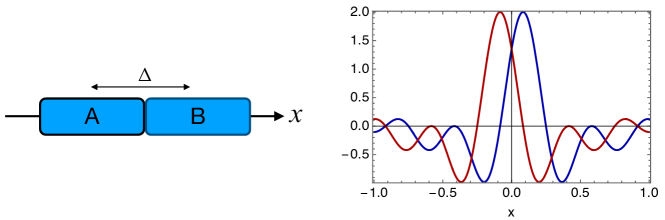
Figure 1: Left panel: setup of spatial regions A and B. Right panel: the window functions for A: $w(x+\Delta/2)$ and B: $w(x-\Delta/2)$ with $k_{0}/k_{c}=0.2$. Although the two window functions overlap, local modes A and B are independent and well-defined as the commutation relation (17) is satisfied.

Covariances for the local operators are calculated as

$$c_{1}(\Delta)=\frac{2}{k_{c}-k_{0}}\int_{k_{0}}^{k_{c}}dk|f_{k}|^{2}\cos k\Delta=\frac{2}{1-\delta}\int_{\delta}^{1}dz|f_{k}|^{2}\cos\left(\frac{\pi z}{1+\delta}\right),$$ (26)

$$c_{2}(\Delta)=\frac{2}{k_{c}-k_{0}}\int_{k_{0}}^{k_{c}}dk|g_{k}|^{2}\cos k\Delta=\frac{2}{1-\delta}\int_{\delta}^{1}dz|g_{k}|^{2}\cos\left(\frac{\pi z}{1+\delta}\right),$$ (27)

$$c_{3}(\Delta)=\frac{1}{k_{c}-k_{0}}\int_{k_{0}}^{k_{c}}dk\,i(f_{k}g_{k}^{*}-f_{k}^{*}g_{k})\cos(k\Delta)=\frac{1}{1-\delta}\int_{\delta}^{1}dz\,i(f_{k}g_{k}^{*}-f_{k}^{*}g_{k})\cos\left(\frac{\pi z}{1+\delta}\right),$$ (28)

where $z=k/k_{c},\delta=k_{0}/k_{c}$. The parameter $\delta$ represents the size of the local region normalized by the total system size: $\delta=(k_{0}\Delta/\pi)(1-k_{0}\Delta/\pi)^{-1}$.

The covariance matrix of the bipartite system AB defined by $(\hat{q}_{\text{A}},\hat{p}_{\text{A}},\hat{q}_{\text{B}},\hat{p}_{\text{B}})$ is given by

$$\boldsymbol{m}_{\text{AB}}=\begin{bmatrix}a_{1}&a_{3}&c_{1}&c_{3}\\ a_{3}&a_{2}&c_{3}&c_{2}\\ c_{1}&c_{3}&a_{1}&a_{3}\\ c_{3}&c_{2}&a_{3}&a_{2}\end{bmatrix},$$ (29)

where $a_{i}:=c_{i}(\Delta=0)$ for $i=1,2,3$. Owing to the homogeneity of the universe represented by the metric (2), the covariance matrices of each mode A and B have the same components; i.e., the bipartite system AB is in a symmetric Gaussian state. Symplectic eigenvalues of the covariance matrix $\boldsymbol{m}_{\text{AB}}$ are calculated as

$$(\nu_{1})^{2}=a_{1}a_{2}-a_{3}^{2}+c_{1}c_{2}-c_{3}^{2}+|a_{1}c_{2}+a_{2}c_{1}-2a_{3}c_{3}|,$$ (30)

$$(\nu_{2})^{2}=a_{1}a_{2}-a_{3}^{2}+c_{1}c_{2}-c_{3}^{2}-|a_{1}c_{2}+a_{2}c_{1}-2a_{3}c_{3}|.$$ (31)

The state represented by the covariance matrix (29) is physical, i.e., positive-semidefinite, if and only if $1\leq\nu_{2}\leq\nu_{1}$.

The partially transposed covariance matrix, which is obtained by reversing the sign of mode B’s momentum, has the following two symplectic eigenvalues:

$$(\tilde{\nu}_{1})^{2}=a_{1}a_{2}-a_{3}^{2}-c_{1}c_{2}+c_{3}^{2}+|(a_{1}c_{2}-a_{2}c_{1})^{2}+4(a_{1}c_{3}-a_{3}c_{3})(a_{2}c_{3}-a_{3}c_{2})|^{1/2},$$ (32)

$$(\tilde{\nu}_{2})^{2}=a_{1}a_{2}-a_{3}^{2}-c_{1}c_{2}+c_{3}^{2}-|(a_{1}c_{2}-a_{2}c_{1})^{2}+4(a_{1}c_{3}-a_{3}c_{3})(a_{2}c_{3}-a_{3}c_{2})|^{1/2}.$$ (33)

Based on the positivity criterion of the partially transposed covariance matrix for a bipartite Gaussian state [26, 27, 28], the negativity gives a measure of entanglement between modes A and B, which is defined as [29, 30]

$$N_{\text{A:B}}:=\frac{1}{2}\mathrm{max}\left(\frac{1}{\tilde{\nu}_{2}}-1,0\right).$$ (34)

The modes A and B are entangled if $N_{\text{A:B}}>0$, while the modes A and B are separable if $N_{\text{A:B}}=0$.

II.2 Entanglement of local modes in the de Sitter universe

We adopt the de Sitter expansion of the scale factor $a_{\text{sc}}=-1/(H\eta),-\infty<\eta<0$, where $H$ is the Hubble constant. Mode functions corresponding to the Bunch-Davies vacuum state, which coincides with the Minkowski vacuum state in the short wavelength limit, are given by

$$f_{k}=\frac{1}{\sqrt{2|k|}}\left(1+\frac{1}{i|k|\eta}\right)e^{-i|k|\eta},\quad g_{k}=\sqrt{\frac{|k|}{2}}e^{-i|k|\eta}.$$ (35)

Covariances of the field operators are calculated as

$$M_{11}=\frac{1}{\pi}\int_{0}^{\infty}\frac{dk}{k}\left(1+\frac{1}{k^{2}\eta^{2}}\right)\cos k(x-y),$$ (36)

$$M_{22}=\frac{1}{\pi}\int_{0}^{\infty}dk\,k\cos k(x-y),$$ (37)

$$M_{12}=\frac{1}{\pi\eta}\int_{0}^{\infty}\frac{dk}{k}\cos k(x-y).$$ (38)

We choose the UV and IR cutoff in the window functions as $k_{c}=\pi H/\delta,k_{0}=\pi H$. The IR cutoff represents the physical size of the whole universe $a_{\text{sc}}H^{-1}$ and the UV cutoff represents the physical size of the focusing spatial region $\delta\times a_{\text{sc}}H^{-1},0\leq\delta\leq 1$. Covariances (26), (27), (28) of the local modes are

$$c_{1}=\frac{1}{\pi H}\frac{\delta}{1-\delta}\int_{\delta}^{1}\frac{dz}{z}\left(1+\frac{a_{\text{sc}}^{2}\,\delta^{2}}{\pi^{2}z^{2}}\right)\cos\left(\frac{\pi z}{1+\delta}\right),$$ (39)

$$c_{2}=\frac{\pi H}{\delta(1-\delta)}\int_{\delta}^{1}dzz\cos\left(\frac{\pi z}{1+\delta}\right),$$ (40)

$$c_{3}=-\frac{1}{\pi H}\frac{a_{\text{sc}}H\delta}{1-\delta}\int_{\delta}^{1}\frac{dz}{z}\cos\left(\frac{\pi z}{1+\delta}\right).$$ (41)

The left panel of Fig. 2 shows the evolution of negativity of the bipartite mode AB, with a fixed comoving size $\delta$. The initial nonzero negativity evolves to be zero at some specific value of the scale factor. The physical size of a local region is characterized by $\delta_{p}:=a_{\text{sc}}\delta$. The right panel of Fig. 2 shows the plot of negativity as a function of $(\delta_{p},a_{\text{sc}})$. For a fixed $\delta\in(0,1)$, this figure shows that entanglement (quantum correlation) between the two local modes A and B is lost after the physical size of the comoving region exceeds the Hubble horizon scale and the “classical” behavior of the quantum field emerges [2, 4, 3, 5, 6].

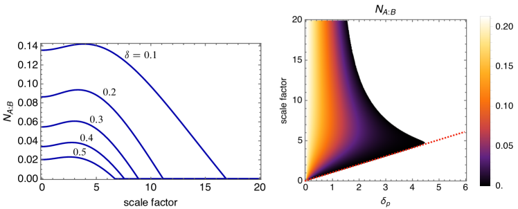
Figure 2: Behavior of negativity. Left panel: dependence on the scale factor with different values of the comoving size $\delta$. Right panel: dependence on the physical size of the local region $\delta_{p}=a_{\text{sc}}\delta$ and the scale factor $a_{\text{sc}}$. The dotted line is $\delta_{p}=a_{\text{sc}}$ that represents the evolution of the total size of the universe. The modes A and B are initially entangled ($a_{\text{sc}}=0$) and become separable after the physical separation between them exceeds the Hubble horizon scale $\sim H^{-1}$ with $k_{c}/a_{\text{sc}}\ll k_{0}$ and the effect of the IR cutoff becomes negligible.

The disentanglement behavior in this figure can be intuitively understood as a result of the fact that “thermal” noise at the Gibbons-Hawking temperature $T_{H}=H/(2\pi)$ associated with the cosmological horizon destroys quantum correlations between A and B. The rest of this paper aims to provide a more quantitative understanding of the disentanglement phenomenon in terms of entanglement monogamy. The bipartite state AB is usually mixed because it is defined as a subsystem embedded in the total universe. As the monogamy relation proposed by Camalet [14, 15, 16, 17, 18] suggests, the amount of quantum correlation between A and B (i.e., internal correlation) is affected by the amount of quantum correlation between AB and its complement (i.e., external correlation). Therefore, we look for the partner modes that purify the bipartite mode AB and investigate the entanglement structure among them in the following sections.

III Purification of local Gaussian modes in quantum fields

To understand the behavior of entanglement between spatial local modes, we look for their partners, i.e., the modes that purify them. In [31], a partner mode of a given mode is calculated in specific examples, including a system with Hawking radiation. A general partner formula that identifies a partner mode for a single mode in any pure Gaussian state is proven in [19]. Generalizing these results, a systematic method to identify any number of modes in a pure state has been developed in [23, 22, 21]. Such a subsystem composed of modes in a pure state is called a quantum information capsule (QIC). Although the QIC formula in [23, 22, 21] provides an algebraic way to identify modes in a pure state, it cannot be directly used for our purpose of analyzing the disentanglement structure of two local modes AB [2, 4, 3, 5] from the viewpoint of monogamy. In this section, we derive a more useful formula to identify the partner modes that purify given two modes AB.

In Sec. III.1, we briefly review the QIC argument with which modes in a pure state are identified. In Sec. III.2, we derive a formula identifying the partner mode of a single mode, which reproduces the partner formula in [19]. In Sec. III.3, we generalize the partner formula to identify the partner of a two-mode system.

III.1 QICs in Gaussian states

The partners here are a special class of QIC. In [23, 22, 21], it has been shown that a linear map, denoted by $f_{\psi}$ for a pure Gaussian state $\ket{\psi}$, plays a key role in identifying a QIC. We here briefly review the results in [23, 22, 21], including the properties of $f_{\psi}$.

Let us first consider a system composed of $N$ harmonic oscillators, which is assumed to be in a pure Gaussian state $\ket{\psi}$. The canonical variables are defined by $\hat{\boldsymbol{r}}=(\hat{q}_{1},\hat{p}_{1},\dots,\hat{q}_{N},\hat{p}_{N})^{T}$. For simplicity, we assume that the first moments of the canonical variables vanish, i.e., $\langle\hat{\boldsymbol{r}}\rangle=0$, where $\langle\,\rangle$ denotes the expectation value in $\ket{\psi}$. The covariance matrix with respect to these canonical variables is defined by $\boldsymbol{m}:=\langle\{\hat{\boldsymbol{r}},\hat{\boldsymbol{r}}^{T}\}\rangle$. Because the total system is assumed to be in a pure Gaussian state, all the symplectic eigenvalues of $\boldsymbol{m}$ are one. That is, there exists a symplectic matrix $\boldsymbol{S}$ such that

$$\boldsymbol{m}=\boldsymbol{S}\boldsymbol{S}^{T},$$ (42)

where $\boldsymbol{S}$ satisfies $\boldsymbol{S}^{T}\boldsymbol{\Omega}_{N}\boldsymbol{S}=\boldsymbol{\Omega}_{N}$ and $[\hat{\boldsymbol{r}},\hat{\boldsymbol{r}}^{T}]=i\boldsymbol{\Omega}_{N}$ for

$$\boldsymbol{\Omega}_{N}:=\bigoplus_{i=1}^{N}\boldsymbol{J},\quad\boldsymbol{J}=\begin{bmatrix}0&1\\ -1&0\end{bmatrix}.$$ (43)

Note that the pure state condition (42) is equivalent to the following relation:

$$\boldsymbol{m}\boldsymbol{\Omega}_{N}\boldsymbol{m}=\boldsymbol{\Omega}_{N}.$$ (44)

If we introduce a new basis $\hat{\boldsymbol{r}}^{\prime}$ for the canonical variables by $\hat{\boldsymbol{r}}^{\prime}=\boldsymbol{S}^{-1}\hat{\boldsymbol{r}}$, we get

$$\boldsymbol{m}^{\prime}=\langle\{\hat{\boldsymbol{r}}^{\prime},\hat{\boldsymbol{r}}^{\prime T}\}\rangle=\boldsymbol{S}\boldsymbol{m}(\boldsymbol{S}^{T})^{-1}=\mathbb{I}_{2N},\quad[\hat{\boldsymbol{r}}^{\prime},\hat{\boldsymbol{r}}^{\prime T}]=i\boldsymbol{\Omega}_{N}.$$ (45)

The canonical variables defined by $\hat{\boldsymbol{r}}^{\prime}$ specify $N$ uncorrelated modes, each of which is in a pure state. Now we define a linear map $f_{\psi}$ by

$$f_{\psi}(\hat{q}_{i}^{\prime})=\hat{p}_{i}^{\prime},\quad f_{\psi}(\hat{p}_{i}^{\prime})=-\hat{q}_{i}^{\prime},$$ (46)

or equivalently,

$$f_{\psi}(\hat{\boldsymbol{r}}^{\prime})=\boldsymbol{\Omega}_{N}\hat{\boldsymbol{r}}^{\prime}.$$ (47)

This map has the following properties:

$$[\hat{\boldsymbol{r}}^{\prime},f_{\psi}(\hat{\boldsymbol{r}}^{\prime})^{T}] =i\mathbb{I}_{2N},$$ (48)

$$\langle\{\hat{\boldsymbol{r}}^{\prime},\hat{\boldsymbol{r}}^{\prime T}\}\rangle =\mathbb{I}_{2N},\quad\langle\{\hat{\boldsymbol{r}}^{\prime},f_{\psi}(\hat{\boldsymbol{r}}^{\prime})^{T}\}\rangle=0,\quad\langle\{f_{\psi}(\hat{\boldsymbol{r}}^{\prime}),f_{\psi}(\hat{\boldsymbol{r}}^{\prime})^{T}\}\rangle=\mathbb{I}_{2N}.$$ (49)

On the one hand, Eq. (48) means that $[\hat{r_{j}}^{\prime},f_{\psi}(\hat{r_{j}}^{\prime})]=i$; i.e., $(\hat{r_{j}}^{\prime},f_{\psi}(\hat{r_{j}}^{\prime}))$ defines a mode for any $j=1,\dots,2N$. On the other hand, Eq. (49) implies that the mode defined by $(\hat{r_{j}}^{\prime},f_{\psi}(\hat{r_{j}}^{\prime}))$ is in a pure state. Of course, these are straightforward consequences of the definition in Eq. (46).

Let us generalize this observation. Consider an operator $\hat{O}$ given by a linear combination of canonical variables. We first rescale this operator as $\hat{O}\to\hat{O}/\sqrt{2\langle\hat{O}^{2}\rangle}$ so that $\langle\hat{O}^{2}\rangle=1/2$. Expanding $\hat{O}$ in the basis $\hat{\boldsymbol{r}}^{\prime}$ as

$$\hat{O}:=\sum_{i=1}^{N}w_{i}^{\prime}\hat{r}_{i}^{\prime}=\boldsymbol{w}^{\prime T}\hat{\boldsymbol{r}}^{\prime},$$ (50)

where $\boldsymbol{w}^{\prime T}=(w_{1}^{\prime},w_{2}^{\prime},\dots,w_{2N}^{\prime})$, the normalization condition is equivalent to

$$\boldsymbol{w}^{\prime T}\boldsymbol{w}^{\prime}=1.$$ (51)

Introducing operators $(\hat{Q},\hat{P}):=(\hat{O},f_{\psi}(\hat{O}))$ for $\hat{O}$ with this normalization, from Eqs. (48), (49) and (51), we find

$$[\hat{Q},\hat{P}] =i$$ (52)

$$\langle\{\hat{Q},\hat{Q}\}\rangle =1,\quad\langle\{\hat{Q},\hat{P}\}\rangle=\langle\{\hat{P},\hat{Q}\}\rangle=0,\quad\langle\{\hat{P},\hat{P}\}\rangle=1.$$ (53)

Equation (52) means that $(\hat{Q},\hat{P})$ satisfies the canonical commutation relation and hence defines a mode. Further, Eq. (53) implies that the covariance matrix for this mode is equal to the $2\times 2$ identity matrix, implying that it is in a pure state.

In a series of studies [32, 23, 22, 21] on the carriers of information, the smallest subsystem in a pure state that carries the whole encoded information is termed a QIC. The encoded information can be fully retrieved by extracting a QIC from the system. Equations (52) and (53) imply that the mode defined by $(\hat{Q},\hat{P}):=(\hat{O},f_{\psi}(\hat{O}))$ is the QIC when the encoding operation is generated by $\hat{O}$. In a more general case where the encoding operation is generated by $\{\hat{O}_{i}\}_{i=1}^{n}$, where each of which is assumed to be a linear combination of canonical variables, it is proven [23] that the QIC is given by a subsystem composed of (at most) $n$ modes, which is algebraically defined by

$$\{(\hat{O}_{i},f_{\psi}(\hat{O}_{i})\}_{i=1}^{n}.$$ (54)

It is shown that operators $\{(\hat{Q}_{i},\hat{P}_{i})\}_{i}$ defined in Eq. (73) in [23] satisfy

$$[\hat{Q}_{j},\hat{P}_{k}] =i\delta_{jk},\quad[\hat{Q}_{j},\hat{Q}_{k}]=[\hat{P}_{j},\hat{P}_{k}]=0$$ (55)

$$\langle\{\hat{Q}_{j},\hat{Q}_{k}\}\rangle =\delta_{jk},\quad\langle\{\hat{Q}_{j},\hat{P}_{k}\}\rangle=\langle\{\hat{P}_{j},\hat{Q}_{k}\}\rangle=0,\quad\langle\{\hat{P}_{j},\hat{P}_{k}\}\rangle=\delta_{jk},$$ (56)

which generalizes Eqs. (55) and (56). It implies that the mode characterized by $\{(\hat{Q}_{i},\hat{P}_{i})\}_{i}$ is in a pure state when the total system is in $\ket{\psi}$, and therefore, they are the QIC as the encoded information is carried by them.

Although the subsystem composed of $n$ modes playing the role of QIC is uniquely determined, there are several ways to decompose it into $n$ independent modes. From Eq. (56), the Gaussian state $\ket{\psi}$ of the total system is decomposed into

$$\ket{\psi}=\ket{\psi^{\prime}}_{12\cdots n}\otimes\ket{\psi^{\prime\prime}}_{\overline{12\cdots n}},\quad\ket{\psi^{\prime}}_{12\cdots n}:=\bigotimes_{j=1}^{n}\ket{0}_{j}$$ (57)

where $\ket{0}_{j}$ denotes the “vacuum” state for the $j$th mode annihilated by $\hat{a}_{j}:=(\hat{Q}_{j}+i\hat{P}_{j})/\sqrt{2}$ and $\ket{\psi^{\prime\prime}}_{\overline{12\cdots n}}$ denotes a pure state for the complementary system. Since each of the $n$ modes is in a pure state in this decomposition, the analysis of the entanglement structure is not straightforward. In the following subsections, we introduce another decomposition that is more useful in analyzing the entanglement structure among partners.

For later convenience, we summarize here the properties of $f_{\psi}$. From the definition in Eq. (47), $f_{\psi}$ maps the original basis $\hat{\boldsymbol{r}}$ to

$$f_{\psi}(\hat{\boldsymbol{r}})=f_{\psi}(\boldsymbol{S}\hat{\boldsymbol{r}}^{\prime})=\boldsymbol{S}\boldsymbol{\Omega}_{N}\boldsymbol{S}^{-1}\hat{\boldsymbol{r}}=\boldsymbol{m}\boldsymbol{\Omega}_{N}\hat{\boldsymbol{r}},$$ (58)

where we have used $\boldsymbol{S}^{-1}=-\boldsymbol{\Omega}_{N}\boldsymbol{S}^{T}\boldsymbol{\Omega}_{N}$. From Eqs. (48) and (49), for any operators $\hat{O}$ and $\hat{O}^{\prime}$ given by linear combinations of canonical operators by (65) [22, 23], it can be directly checked that

$$\langle\hat{O}\rangle=0,\quad\langle f_{\psi}(\hat{O})\rangle=0,\quad f_{\psi}(f_{\psi}(\hat{O}))=-\hat{O}$$ (59)

$$[\hat{O},f_{\psi}(\hat{O}^{\prime})]=i\langle\{\hat{O},\hat{O}^{\prime}\}\rangle,\quad\langle\{\hat{O},f_{\psi}(\hat{O}^{\prime})\}\rangle=i[\hat{O},\hat{O}^{\prime}],$$ (60)

$$[f_{\psi}(\hat{O}),f_{\psi}(\hat{O}^{\prime})]=[\hat{O},\hat{O}^{\prime}],\quad\langle\{f_{\psi}(\hat{O}),f_{\psi}(\hat{O}^{\prime})\}\rangle=\langle\{\hat{O},\hat{O}^{\prime}\}\rangle$$ (61)

hold.

So far, we have reviewed the properties of map $f_{\psi}$ in a harmonic oscillator system. The analyses can readily be extended to a scalar field by the following procedure. For a scalar field $\hat{\varphi}$ and its conjugate momentum $\hat{\pi}$ at a fixed time $t$, we denote

$$\hat{\boldsymbol{R}}(x):=\begin{bmatrix}\hat{\varphi}(t,x)\\ \hat{\pi}(t,x)\end{bmatrix}.$$ (62)

Here, for notational simplicity, we omit the time variable $t$ on the left-hand side. The equal-time commutation relations in Eq. (9) are written as

$$[\hat{\boldsymbol{R}}(x),\hat{\boldsymbol{R}}^{T}\!(y)]=i\begin{bmatrix}0&\delta(x-y)\\ -\delta(x-y)&0\end{bmatrix}=i\boldsymbol{J}\delta(x-y),$$ (63)

where $\boldsymbol{J}=\begin{bmatrix}0&1\\ -1&0\end{bmatrix}$, while the covariance of the field operators in the state $\ket{\psi}$ are denoted by

$$\boldsymbol{M}(x,y):=\langle\{\hat{\boldsymbol{R}}(x),\hat{\boldsymbol{R}}^{T}\!(y)\}\rangle=\begin{bmatrix}M_{11}(x,y)&M_{12}(x,y)\\ M_{21}(x,y)&M_{22}(x,y)\end{bmatrix}=\begin{bmatrix}\langle\{\hat{\varphi}(x),\hat{\varphi}(y)\}\rangle&\langle\{\hat{\varphi}(x),\hat{\pi}(y)\}\rangle\\ \langle\{\hat{\pi}(x),\hat{\varphi}(y)\}\rangle&\langle\{\hat{\pi}(x),\hat{\pi}(y)\}\rangle\end{bmatrix}.$$ (64)

We introduce an operator

$$\hat{O}:=\int dx\left[w_{1}(x)\hat{\varphi}(x)+w_{2}(x)\hat{\pi}(x)\right]=\int dx\boldsymbol{W}^{T}\!(x)\hat{\boldsymbol{R}}(x),$$ (65)

where

$$\boldsymbol{W}(x)=\begin{bmatrix}w_{1}(x)\\ w_{2}(x)\end{bmatrix}$$ (66)

denotes weighting functions. In the analogy with Eq. (58), we define [23] a map $f_{\psi}$ by

$$f_{\psi}(\hat{O}) :=\int dxdydz\boldsymbol{W}^{T}(x)\boldsymbol{M}(x,y)\boldsymbol{J}\delta(y-z)\hat{\boldsymbol{R}}(z)$$

$$=\int dx\boldsymbol{W}_{\!\!\!f_{\psi}(\hat{O})}^{T}(x)\hat{\boldsymbol{R}}(x),$$ (67)

where $\boldsymbol{W}_{\!\!\!f_{\psi}(\hat{O})}$ is the window function defining $f_{\psi}(\hat{O})$, given by

$$\boldsymbol{W}_{\!\!\!f_{\psi}(\hat{O})}(x):=-\int dy\boldsymbol{J}\boldsymbol{M}(x,y)\boldsymbol{W}(y).$$ (68)

When the covariance of the field operator satisfies a purity condition

$$\int dydz\boldsymbol{M}(x,y)\boldsymbol{J}\delta(y-z)\boldsymbol{M}(z,w)=\boldsymbol{J}\delta(x-w),$$ (69)

which corresponds to Eq. (44), it is shown [22, 23] that the map $f_{\psi}$ satisfies all the properties in Eqs. (59), (60) and (61). Therefore, for operators $\{O_{i}\}_{i=1}^{n}$ given by linear combinations of field operators, the set of operators

$$\{(\hat{O}_{i},f_{\psi}(\hat{O}_{i})\}_{i=1}^{n}$$ (70)

defines (at most) $n$ modes in a pure state, provided that the field is in a pure Gaussian state $\ket{\psi}$. Note that Eq. (69) can be explicitly confirmed for the covariances given in Eqs. (36), (37) and (38).

Based on these results, we derive the partner formula for a single mode in Sec. III.2, which reproduces the formula in [19]. We further generalize it for the partner formula for two modes in Sec. III.3, which we shall use to analyze entanglement monogamy among local modes in a field. See Fig. 3 for the schematic picture of these setups.

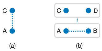
Figure 3: (a) Purification of a single mode A. The mode C is a partner of A. (b) Purification of two modes AB. The modes C and D are partners of the bipartite system AB.

III.2 Purification of a single Gaussian mode

As a practical application of the map $f_{\psi}$, we look for a partner mode that purifies a given single mode A [Fig. 3 (a)]. In particular, we apply the partner formula for a local mode $\hat{\boldsymbol{\xi}}_{\text{A}}=(\hat{q}_{\text{A}},\hat{p}_{\text{A}})^{T}$ at a spatial point ${\boldsymbol{x}}_{\text{A}}$ defined in the previous section. As we have seen in Sec. III.1, four operators

$$\hat{q}_{\text{A}},\hat{p}_{\text{A}},f_{\psi}(\hat{q}_{\text{A}}),f_{\psi}(\hat{p}_{\text{A}}),$$ (71)

define a two-mode system that is in a pure state, provided that the field is in a pure Gaussian state. To identify the partner mode of $\hat{\boldsymbol{\xi}}_{\text{A}}$, we here construct a mode generated by the operators in Eq. (71), which is orthonormal to the mode A. The covariance matrix for $\hat{\boldsymbol{\xi}}_{\text{A}}$ is

$$\boldsymbol{m}_{\text{A}}:=\expectationvalue{\{\hat{\boldsymbol{\xi}}_{\text{A}},\hat{\boldsymbol{\xi}}^{T}_{\text{A}}\}}=\begin{bmatrix}2\expectationvalue{\hat{q}_{\text{A}}^{2}}&\expectationvalue{\hat{q}_{\text{A}}\hat{p}_{\text{A}}+\hat{p}_{\text{A}}\hat{q}_{\text{A}}}\\ \expectationvalue{\hat{q}_{\text{A}}\hat{p}_{\text{A}}+\hat{p}_{\text{A}}\hat{q}_{\text{A}}}&2\expectationvalue{\hat{p}_{\text{A}}^{2}}\end{bmatrix}=\begin{bmatrix}c_{1}&c_{3}\\ c_{3}&c_{2}\end{bmatrix}.$$ (72)

Commutators and covariances between these operators are given by

$$[\hat{\boldsymbol{\xi}}_{\text{A}},\hat{\boldsymbol{\xi}}^{T}_{\text{A}}]=[f_{\psi}(\hat{\boldsymbol{\xi}}_{\text{A}}),f_{\psi}(\hat{\boldsymbol{\xi}}^{T}_{\text{A}})]=i\boldsymbol{J},\quad[\hat{\boldsymbol{\xi}}_{\text{A}},f_{\psi}(\hat{\boldsymbol{\xi}}^{T}_{\text{A}})]=i\boldsymbol{m}_{\text{A}},$$ (73)

and

$$\expectationvalue{\{\hat{\boldsymbol{\xi}}_{\text{A}},\hat{\boldsymbol{\xi}}^{T}_{\text{A}}\}}=\expectationvalue{\{f_{\psi}(\hat{\boldsymbol{\xi}}_{\text{A}}),f_{\psi}(\hat{\boldsymbol{\xi}}^{T}_{\text{A}})\}}=\boldsymbol{m}_{\text{A}},\quad\expectationvalue{\{\hat{\boldsymbol{\xi}}_{\text{A}},f_{\psi}(\hat{\boldsymbol{\xi}}^{T}_{\text{A}})\}}=-\boldsymbol{J}.$$ (74)

To extract a mode orthogonal to the original mode $\hat{\boldsymbol{\xi}}_{\text{A}}$ from $f_{\psi}(\hat{\boldsymbol{\xi}}_{\text{A}})$, we define operators

$$\hat{\boldsymbol{\zeta}}:=f_{\psi}(\hat{\boldsymbol{\xi}}_{\text{A}})-\boldsymbol{m}_{\text{A}}\boldsymbol{J}\hat{\boldsymbol{\xi}}_{\text{A}}.$$ (75)

They indeed commute with $\hat{\boldsymbol{\xi}}_{\text{A}}$ as

$$[\hat{\boldsymbol{\zeta}},\hat{\boldsymbol{\xi}}^{T}_{\text{A}}] =[f_{\psi}(\hat{\boldsymbol{\xi}}_{\text{A}}),\hat{\boldsymbol{\xi}}^{T}_{\text{A}}]-[\boldsymbol{m}_{\text{A}}\boldsymbol{J}\hat{\boldsymbol{\xi}}_{\text{A}},\hat{\boldsymbol{\xi}}^{T}_{\text{A}}]$$

$$=-\boldsymbol{m}_{\text{A}}-\boldsymbol{m}_{\text{A}}\boldsymbol{J}[\hat{\boldsymbol{\xi}}_{\text{A}},\hat{\boldsymbol{\xi}}^{T}_{\text{A}}]$$

$$=0.$$ (76)

Therefore, they define a mode orthogonal to $\hat{\boldsymbol{\xi}}_{\text{A}}$.

The commutator of $\hat{\boldsymbol{\zeta}}$ is calculated as

$$[\hat{\boldsymbol{\zeta}},\hat{\boldsymbol{\zeta}}^{T}] =i(\boldsymbol{J}-\boldsymbol{m}_{\text{A}}\boldsymbol{J}\boldsymbol{m}_{\text{A}}).$$ (77)

If the mode A is in a pure state, it holds $\boldsymbol{m}_{\text{A}}\boldsymbol{J}\boldsymbol{m}_{\text{A}}=\boldsymbol{J}$ which corresponds to the relation of the density operator $\hat{\rho}^{2}_{\text{A}}=\hat{\rho}_{\text{A}}$, implying that the commutator of $\hat{\boldsymbol{\zeta}}$ is trivial. In this case, because $\hat{\boldsymbol{\xi}}_{\text{A}}$ is in a pure state, its partner mode does not exist. If the mode A is not pure, its partner is characterized by $\hat{\boldsymbol{\zeta}}$. We normalize $\hat{\boldsymbol{\zeta}}$ to make it a canonical pair of operators. For this purpose, we introduce $\hat{\boldsymbol{\xi}}_{\text{C}}$ by $\hat{\boldsymbol{\zeta}}=\boldsymbol{A}\,\hat{\boldsymbol{\xi}}_{\text{C}}$ with a matrix $\boldsymbol{A}$ so that $[\hat{\boldsymbol{\xi}}_{\text{C}},\hat{\boldsymbol{\xi}}_{\text{C}}^{T}]=i\boldsymbol{J}$ holds. The condition on the matrix $\boldsymbol{A}$ is given by

$$\boldsymbol{AJA}^{T}=\boldsymbol{J}-\boldsymbol{m}_{\text{A}}\boldsymbol{J}\boldsymbol{m}_{\text{A}}.$$ (78)

To obtain $\boldsymbol{A}$, we consider the standard form of the covariance matrix $\boldsymbol{m}_{\text{A}}$:

$$\boldsymbol{m}_{\text{A}}=\boldsymbol{S}\begin{bmatrix}a&0\\ 0&a\end{bmatrix}\boldsymbol{S}^{T}=a\boldsymbol{S}\boldsymbol{S}^{T},\quad\boldsymbol{SJS^{T}}=\boldsymbol{J},$$ (79)

where $\boldsymbol{S}$ represents a symplectic transformation to diagonalize $\boldsymbol{m}_{\text{A}}$ and $a$ is the symplectic eigenvalue of $\boldsymbol{m}_{\text{A}}$.

Although the partner mode C itself is unique, the matrix $\boldsymbol{S}$ satisfying Eq. (78) is not uniquely determined because of the remaining freedom in fixing a canonical set of operators for the mode C. In other words, when $\boldsymbol{A}$ satisfies Eq. (78), so does $\boldsymbol{A}^{\prime}:=\boldsymbol{S}^{\prime}\boldsymbol{A}$, where $\boldsymbol{S}^{\prime}$ is an arbitrary $2\times 2$ symplectic matrix. Since Eq. (78) is recast into $\boldsymbol{AJA}^{T}=(1-a^{2})\boldsymbol{J}$, we can choose

$$\boldsymbol{A}=\sqrt{a^{2}-1}\,\boldsymbol{X},$$ (80)

or equivalently

$$\boldsymbol{A}^{-1}=\frac{1}{\sqrt{a^{2}-1}}\boldsymbol{X},\quad$$ (81)

where $\boldsymbol{X}=\begin{bmatrix}0&1\\ 1&0\end{bmatrix}$.

In summary, the partner mode C of mode A is obtained as the following formula:

$$\hat{\boldsymbol{\xi}}_{\text{C}} =\boldsymbol{A}^{-1}\hat{\boldsymbol{\zeta}}=\frac{1}{\sqrt{a^{2}-1}}\boldsymbol{X}(f_{\psi}(\hat{\boldsymbol{\xi}}_{\text{A}})-\boldsymbol{m}_{\text{A}}\boldsymbol{J}\hat{\boldsymbol{\xi}}_{\text{A}})$$

$$=\frac{1}{\sqrt{a^{2}-1}}\begin{bmatrix}c_{2}\hat{q}_{\text{A}}-c_{3}\hat{p}_{\text{A}}+f_{\psi}(\hat{p}_{\text{A}})\\ c_{3}\hat{q}_{\text{A}}-c_{1}\hat{p}_{\text{A}}+f_{\psi}(\hat{q}_{\text{A}})\end{bmatrix}=:\begin{bmatrix}\hat{q}_{\text{C}}\\ \hat{p}_{\text{C}}\end{bmatrix},$$ (82)

which is equivalent to the partner formula for a single mode [19] in a Gaussian state. Covariances of operators $(\hat{\boldsymbol{\xi}}_{\text{A}},\hat{\boldsymbol{\xi}}_{\text{C}})$ are given by

$$\expectationvalue{\{\hat{\boldsymbol{\xi}}_{\text{A}},\hat{\boldsymbol{\xi}}_{\text{A}}^{T}\}} =\boldsymbol{m}_{\text{A}},$$ (83)

$$\expectationvalue{\{\hat{\boldsymbol{\xi}}_{\text{C}},\hat{\boldsymbol{\xi}}_{\text{A}}^{T}\}} =\boldsymbol{A}^{-1}(\boldsymbol{J}-\boldsymbol{m}_{\text{A}}\boldsymbol{J}\boldsymbol{m}_{\text{A}})=\sqrt{a^{2}-1}\boldsymbol{Z},$$ (84)

$$\expectationvalue{\{\hat{\boldsymbol{\xi}}_{\text{C}},\hat{\boldsymbol{\xi}}_{\text{C}}^{T}\}} =-\boldsymbol{A}^{-1}(\boldsymbol{m}_{\text{A}}+\boldsymbol{m}_{\text{A}}\boldsymbol{J}\boldsymbol{m}_{\text{A}}\boldsymbol{J}\boldsymbol{m}_{\text{A}})(\boldsymbol{A}^{-1})^{T}=\boldsymbol{X}\boldsymbol{m}_{\text{A}}\boldsymbol{X},$$ (85)

where $\boldsymbol{Z}=\begin{bmatrix}1&0\\ 0&-1\end{bmatrix}$. In a matrix form, they are summarized as

$$\boldsymbol{m}_{\text{AC}}:=\expectationvalue{\{\hat{\boldsymbol{\xi}}_{\text{AC}},\hat{\boldsymbol{\xi}}_{\text{AC}}^{T}\}}=\begin{bmatrix}\boldsymbol{m}_{\text{A}}&\sqrt{a^{2}-1}\boldsymbol{Z}\\ \sqrt{a^{2}-1}\boldsymbol{Z}&\boldsymbol{X}\boldsymbol{m}_{\text{A}}\boldsymbol{X}\end{bmatrix},\quad\hat{\boldsymbol{\xi}}_{\text{AC}}:=\begin{bmatrix}\hat{\boldsymbol{\xi}}_{\text{A}}\\ \hat{\boldsymbol{\xi}}_{\text{C}}\end{bmatrix}.$$ (86)

One can explicitly confirm that this covariance matrix satisfies the following purity condition of the state AC:

$$\boldsymbol{m}_{\text{AC}}\,\boldsymbol{\Omega}_{2}\,\boldsymbol{m}_{\text{AC}}=\boldsymbol{\Omega}_{2},\quad\boldsymbol{\Omega}_{2}=\bigoplus_{i=1}^{2}\boldsymbol{J},$$ (87)

implying that it represents a pure two-mode squeezed state characterizing the pair of partners AC. The total state is decomposed as

$$\ket{\psi}=\ket{\psi^{\prime}}_{\text{AC}}\otimes\ket{\psi^{\prime\prime}}_{\overline{\text{AC}}},$$ (88)

where $\ket{\psi^{\prime}}_{\text{AC}}$ is the pure Gaussian state defined by $\boldsymbol{m}_{\text{AC}}$ and has no correlation with its complement system $\overline{\text{AC}}$ in another pure state $\ket{\psi^{\prime\prime}}_{\overline{\text{AC}}}$.

Spatial profile of partner mode.

Using Eq. (68), the spatial profiles of the partner mode can be visualized. As a window function of local mode A, we adopt $\boldsymbol{W}_{\!\!q_{\text{A}}}=w_{\text{A}}(x)(1,0)^{T}$ and $\boldsymbol{W}_{\!\!p_{\text{A}}}=w_{\text{A}}(x)(0,1)^{T}$, which we have used to introduce local modes from the scalar field in (14) and (15). From Eq. (68), we get

$$\boldsymbol{W}_{\!\!\!f_{\psi}(q_{\text{A}})}(x)=-\int dy\begin{bmatrix}M_{12}(x,y)&M_{22}(x,y)\\ -M_{11}(x,y)&-M_{12}(x,y)\end{bmatrix}\begin{bmatrix}w_{\text{A}}(y)\\ 0\end{bmatrix}=\int dy\begin{bmatrix}-M_{12}(x,y)\\ M_{11}(x,y)\end{bmatrix}w_{\text{A}}(y),$$ (89)

$$\boldsymbol{W}_{\!\!\!f_{\psi}(p_{\text{A}})}(x)=-\int dy\begin{bmatrix}M_{12}(x,y)&M_{22}(x,y)\\ -M_{11}(x,y)&-M_{12}(x,y)\end{bmatrix}\begin{bmatrix}0\\ w_{\text{A}}(y)\end{bmatrix}=\int dy\begin{bmatrix}-M_{22}(x,y)\\ M_{12}(x,y)\end{bmatrix}w_{\text{A}}(y),$$ (90)

and

$$f_{\psi}(\hat{q}_{\text{A}})=\int dx\boldsymbol{W}_{\!\!\!f_{\psi}(q_{\text{A}})}^{T}(x)\hat{\boldsymbol{R}}(x)=\int dxdy\left[-\hat{\varphi}(x)M_{12}(x,y)w_{\text{A}}(y)+\hat{\pi}(x)M_{11}(x,y)w_{\text{A}}(y)\right],$$ (91)

$$f_{\psi}(\hat{p}_{\text{A}})=\int dx\boldsymbol{W}_{\!\!\!f_{\psi}(p_{\text{A}})}^{T}(x)\hat{\boldsymbol{R}}(x)=\int dxdy\left[-\hat{\varphi}(x)M_{22}(x,y)w_{\text{A}}(y)+\hat{\pi}(x)M_{12}(x,y)w_{\text{A}}(y)\right].$$ (92)

In other words, the window functions of $f_{\psi}(\hat{\boldsymbol{\xi}}_{\text{A}})$ are expressed by convolutions of the window function $w_{\text{A}}$ with the covariance matrix $M_{ij}$ of the field operators, given by

$$\int dyM_{11}(x,y)w_{\text{A}}(y) =\frac{4}{\sqrt{\pi(k_{c}-k_{0})}}\int_{k_{0}}^{k_{c}}dk|f_{k}|^{2}\cos k(x-x_{\text{A}})$$

$$=\frac{2}{\pi\sqrt{H}}\sqrt{\frac{\delta}{1-\delta}}\int_{\delta}^{1}\frac{dz}{z}\left(1+\frac{a_{\text{sc}}^{2}\,\delta^{2}}{\pi^{2}z^{2}}\right)\cos\left(z\frac{\pi H(x-x_{\text{A}})}{\delta}\right),$$ (93)

$$\int dyM_{22}(x,y)w_{\text{A}}(y) =\frac{4}{\sqrt{\pi(k_{c}-k_{0})}}\int_{k_{0}}^{k_{c}}dk|g_{k}|^{2}\cos k(x-x_{\text{A}})$$

$$=\frac{2}{\pi\sqrt{H}}\sqrt{\frac{\delta}{1-\delta}}\left(\frac{\pi H}{\delta}\right)^{2}\int_{\delta}^{1}dzz\cos\left(z\frac{\pi H(x-x_{\text{A}})}{\delta}\right),$$ (94)

$$\int dyM_{12}(x,y)w_{\text{A}}(y) =\frac{2}{\sqrt{\pi(k_{c}-k_{0})}}\int_{k_{0}}^{k_{c}}dk\,i(f_{k}g_{k}^{*}-f_{k}^{*}g_{k})\cos k(x-x_{\text{A}})$$

$$=-\frac{2}{\pi\sqrt{H}}\sqrt{\frac{\delta}{1-\delta}}\,(a_{\text{sc}}H)\int_{\delta}^{1}\frac{dz}{z}\cos\left(z\frac{\pi H(x-x_{\text{A}})}{\delta}\right).$$ (95)

From these equations, we obtain spatial profiles of the partner mode C. The upper panel of Fig. 4 shows the window function of the mode A with $\delta=0.1$ as a function of the physical coordinate $x_{p}:=a_{\text{sc}}\,x$ (we set $H=1$). Because of cosmic expansion, the width of the window function (spatial size of the local mode A) increases from $0.1H^{-1}$ to $H^{-1}$. The lower panels are the convolution of $w$ with the covariance of field operators, which appear in the partner formulas (91) and (92). As we can observe from the behavior of convolutions with $M_{11},M_{12}$, amplitudes of these functions become larger as the universe expands and typical wavelengths become $\sim 10H^{-1}$ which is far larger than the width of $w_{\text{A}}$; this behavior of the partner’s window functions implies that the information of the original mode A shared with its partner C delocalizes and extends over the superhorizon scale. These facts provide the following intuitive understanding of the mechanism of disentanglement between local modes: Because the partner of a local mode A is spread over the superhorizon scale for a large scale factor, it is slightly different from another local mode B, implying that modes AB cannot share much entanglement. This observation becomes more quantitative in Sec. IV, where we analyze the disentanglement from the viewpoint of entanglement monogamy.

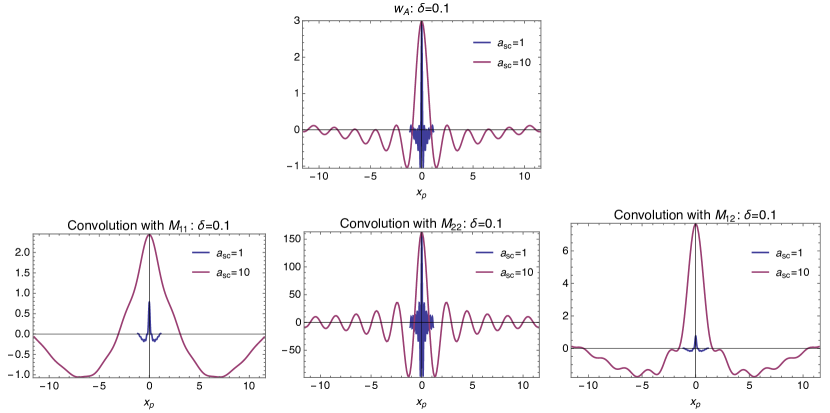
Figure 4: Upper panel: the window function $w_{\text{A}}$ that represents the spatial profile of mode A at $a_{\text{sc}}=1,10$. We set $x_{\text{A}}=0$. $x_{p}=a_{\text{sc}}\,x$ denotes the physical coordinate. Owing to cosmic expansion, the width of the profile increases as $a_{\text{sc}}\delta$. Lower panels: convolution of $w_{\text{A}}$ with covariances of the field operators. These functions represent spatial profiles of the partner mode C.

Negativity between AC.

The standard form of the covariance matrix for the mode A is

$$\boldsymbol{m}_{\text{A}}=\begin{bmatrix}a&0\\ 0&a\end{bmatrix},$$ (96)

where $a$ is the symplectic eigenvalue of $\boldsymbol{m}_{\text{A}}$. As shown in Eq. (86), the covariance matrix of A and its partner C is given by

$$\boldsymbol{m}_{\text{AC}}=\begin{bmatrix}a&0&\sqrt{a^{2}-1}&0\\ 0&a&0&-\sqrt{a^{2}-1}\\ \sqrt{a^{2}-1}&0&a&0\\ 0&-\sqrt{a^{2}-1}&0&a\end{bmatrix}.$$ (97)

The smaller symplectic eigenvalue of its partial transposition of $\boldsymbol{m}_{\text{AC}}$ is calculated as

$$\widetilde{\nu}_{2}=a-\sqrt{a^{2}-1}=\frac{1}{a+\sqrt{a^{2}-1}}\leq 1.$$ (98)

Thus the negativity between the modes A and C is given by

$$N_{\text{A:C}}=\frac{1}{2}(a+\sqrt{a^{2}-1}-1)\geq 0.$$ (99)

For $a>1$, the bipartite state AC is entangled. Figure 5 shows the behavior of the symplectic eigenvalue $a=\sqrt{a_{1}a_{2}-a_{3}^{2}}$ as functions of the scale factor and $\delta$, where $a_{1},a_{2},a_{3}$ are components of the covariance matrix (29). The left panel of Fig. 5 shows that for a fixed value of $\delta$, the symplectic eigenvalue $a$ and the negativity between AC increase as the scale factor increases. The right panel of Fig. 5 shows that for a fixed value of scale factor $a_{\text{sc}}$, the symplectic eigenvalue $a$ increases as the size $\delta$ of the region A decreases. Thus the state AC is more squeezed for a smaller value of $\delta$. In the limit of $\delta\to 1$, the negativity $N_{\text{A:C}}$ vanishes since $a\to 1$, implying that the purity of the state of mode $A$ approaches one.

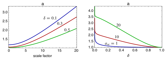
Figure 5: Behavior of the symplectic eigenvalue $a$. Left panel: dependence on the scale factor. The symplectic eigenvalue $a$ is an increasing function of the scale factor and entanglement between AC grows as the universe expands. Right panel: dependence on the normalized comoving size $\delta$ of the region A.

In terms of the symplectic eigenvalue $a$, the entanglement entropy of the mode A is given by

$$S_{\text{A}}=\left(\frac{a+1}{2}\right)\log_{2}\left(\frac{a+1}{2}\right)-\left(\frac{a-1}{2}\right)\log_{2}\left(\frac{a-1}{2}\right).$$ (100)

As the symplectic eigenvalue $a$ monotonically increases with the scale factor, the entanglement entropy of the mode A also increases with the scale factor. Thus the information shared between two modes A and C increases because the mixedness of the state A grows. This explains the delocalization of the information stored in A and the spread of the partner’s window function as visualized in Fig. 4. In the limit of $\delta\rightarrow 1$, $S_{\text{A}}$ approaches zero and A and C share no information.

III.3 Purification of the bipartite Gaussian mode

In this subsection, we construct partner modes CD for the two-mode system $\hat{\boldsymbol{\xi}}_{\text{AB}}=(\hat{q}_{\text{A}},\hat{p}_{\text{A}},\hat{q}_{\text{B}},\hat{p}_{\text{B}})^{T}$. See Fig. 3 (b) for the schematic picture of the setup. To the authors’ knowledge, an explicit formula to obtain the partner modes of a two-mode system has not yet appeared in the literature. Therefore, we explain here the derivation, although it is quite similar to the arguments in the previous subsection, i.e., the derivation of the partner formula for a one-mode system.

From the arguments in Sec. III.1, the eight operators $\hat{\boldsymbol{\xi}}_{\text{AB}}$ and $f_{\psi}(\hat{\boldsymbol{\xi}}_{\text{AB}})$, i.e.,

$$\hat{q}_{\text{A}},\hat{p}_{\text{A}},\hat{q}_{\text{B}},\hat{p}_{\text{B}},f_{\psi}(\hat{q}_{\text{A}}),f_{\psi}(\hat{p}_{\text{A}}),f_{\psi}(\hat{q}_{\text{B}}),f_{\psi}(\hat{p}_{\text{B}})$$ (101)

define a system composed of four modes ABCD, which is in a pure state. We aim to construct two modes CD orthonormal to modes AB. Commutators between these operators are given by

$$[\hat{\boldsymbol{\xi}}_{\text{AB}},\hat{\boldsymbol{\xi}}_{\text{AB}}^{T}]=i\boldsymbol{\Omega}_{2},\quad[\hat{\boldsymbol{\xi}}_{\text{AB}},f_{\psi}(\hat{\boldsymbol{\xi}}_{\text{AB}}^{T})]=i\boldsymbol{m}_{\text{AB}},\quad[f_{\psi}(\hat{\boldsymbol{\xi}}_{\text{AB}}),\hat{\boldsymbol{\xi}}_{\text{AB}}^{T}]=-i\boldsymbol{m}_{\text{AB}},\quad[f_{\psi}(\hat{\boldsymbol{\xi}}_{\text{AB}}),f_{\psi}(\hat{\boldsymbol{\xi}}_{\text{AB}}^{T})]=i\boldsymbol{\Omega}_{2},$$ (102)

where $\boldsymbol{m}_{\text{AB}}$ denotes the covariance matrix for the two mode system $\hat{\boldsymbol{\xi}}_{\text{AB}}$:

$$\boldsymbol{m}_{\text{AB}}:=\expectationvalue{\{\hat{\boldsymbol{\xi}}_{\text{AB}},\hat{\boldsymbol{\xi}}^{T}_{\text{AB}}\}}=\expectationvalue{\{f_{\psi}(\hat{\boldsymbol{\xi}}_{\text{AB}}),f_{\psi}(\hat{\boldsymbol{\xi}}_{\text{AB}}^{T})\}},\quad\expectationvalue{\left\{\hat{\boldsymbol{\xi}}_{\text{AB}},f_{\psi}(\hat{\boldsymbol{\xi}}_{\text{AB}}^{T})\right\}}=-\boldsymbol{\Omega}_{2}.$$ (103)

To find modes orthogonal to the original mode $\hat{\boldsymbol{\xi}}_{\text{AB}}$, we introduce operators

$$\hat{\boldsymbol{\zeta}}:=f_{\psi}(\hat{\boldsymbol{\xi}}_{\text{AB}})-\boldsymbol{m}_{\text{AB}}\,\boldsymbol{\Omega}_{2}\,\hat{\boldsymbol{\xi}}_{\text{AB}}.$$ (104)

They satisfy $[\hat{\boldsymbol{\zeta}},\hat{\boldsymbol{\xi}}_{\text{AB}}^{T}]=0$ since

$$[\hat{\boldsymbol{\zeta}},\hat{\boldsymbol{\xi}}_{\text{AB}}^{T}] =[f_{\psi}(\hat{\boldsymbol{\xi}}_{\text{AB}}),\hat{\boldsymbol{\xi}}_{\text{AB}}^{T}]-[\boldsymbol{m}_{\text{AB}}\,\boldsymbol{\Omega}_{2}\,\hat{\boldsymbol{\xi}}_{\text{AB}},\hat{\boldsymbol{\xi}}_{\text{AB}}]$$

$$=-i\boldsymbol{m}_{\text{AB}}-\boldsymbol{m}_{\text{AB}}\,\boldsymbol{\Omega}_{2}[\hat{\boldsymbol{\xi}}_{\text{AB}},\hat{\boldsymbol{\xi}}_{\text{AB}}^{T}]$$

$$=0$$ (105)

and therefore define modes orthogonal to the original modes AB. The commutators and the covariances for $\hat{\boldsymbol{\zeta}}$ are calculated as

$$[\hat{\boldsymbol{\zeta}},\hat{\boldsymbol{\zeta}}^{T}]=i(\boldsymbol{\Omega}_{2}-\boldsymbol{m}_{\text{AB}}\,\boldsymbol{\Omega}_{2}\,\boldsymbol{m}_{\text{AB}}),\quad\expectationvalue{\left\{\hat{\boldsymbol{\zeta}},\hat{\boldsymbol{\zeta}}^{T}\right\}}=-\left(\boldsymbol{m}_{\text{AB}}+\boldsymbol{m}_{\text{AB}}\,\boldsymbol{\Omega}_{2}\,\boldsymbol{m}_{\text{AB}}\,\boldsymbol{\Omega}_{2}\,\boldsymbol{m}_{\text{AB}}\right).$$ (106)

If $\boldsymbol{\Omega}_{2}=\boldsymbol{m}_{\text{AB}}\,\boldsymbol{\Omega}_{2}\,\boldsymbol{m}_{\text{AB}}$, the two-mode system AB is in a pure state, implying their partners do not exist. We therefore assume that $\boldsymbol{\Omega}_{2}\neq\boldsymbol{m}_{\text{AB}}\,\boldsymbol{\Omega}_{2}\,\boldsymbol{m}_{\text{AB}}$. We normalize $\hat{\boldsymbol{\zeta}}$ as $\hat{\boldsymbol{\zeta}}=\boldsymbol{A}\,\hat{\boldsymbol{\xi}}_{\text{CD}}$ using a matrix $\boldsymbol{A}$ so that the standard canonical commutation relation for modes C and D

$$\quad[\hat{\boldsymbol{\xi}}_{\text{CD}},\hat{\boldsymbol{\xi}}_{\text{CD}}^{T}]=i\boldsymbol{\Omega}_{2}$$ (107)

is satisfied. This is equivalent to a constraint on the $4\times 4$ matrix $\boldsymbol{A}$ given by

$$\boldsymbol{A\Omega}_{2}\boldsymbol{A}^{T}=\boldsymbol{\Omega}_{2}-\boldsymbol{m}_{\text{AB}}\,\boldsymbol{\Omega}_{2}\,\boldsymbol{m}_{\text{AB}}.$$ (108)

By using matrix $\boldsymbol{A}$ satisfying this condition, covariances of normalized operators $\hat{\boldsymbol{\xi}}_{\text{CD}}$ are expressed as

$$\expectationvalue{\left\{\hat{\boldsymbol{\xi}}_{\text{CD}},\hat{\boldsymbol{\xi}}_{\text{CD}}^{T}\right\}} =\boldsymbol{A}^{-1}\expectationvalue{\left\{\hat{\boldsymbol{\zeta}},\hat{\boldsymbol{\zeta}}^{T}\right\}}(\boldsymbol{A}^{-1})^{T}$$

$$=-\boldsymbol{A}^{-1}(\boldsymbol{m}_{\text{AB}}+\boldsymbol{m}_{\text{AB}}\,\boldsymbol{\Omega}_{2}\,\boldsymbol{m}_{\text{AB}}\,\boldsymbol{\Omega}_{2}\,\boldsymbol{m}_{\text{AB}})(\boldsymbol{A}^{-1})^{T}=:\boldsymbol{m}_{\text{CD}},$$ (109)

$$\expectationvalue{\left\{\hat{\boldsymbol{\xi}}_{\text{CD}},\hat{\boldsymbol{\xi}}_{\text{AB}}^{T}\right\}} =\boldsymbol{A}^{-1}(\boldsymbol{\Omega}_{2}-\boldsymbol{m}_{\text{AB}}\,\boldsymbol{\Omega}_{2}\,\boldsymbol{m}_{\text{AB}})=:\boldsymbol{m}_{\text{AB,CD}}^{T},$$ (110)

$$\expectationvalue{\left\{\hat{\boldsymbol{\xi}}_{\text{AB}},\hat{\boldsymbol{\xi}}_{\text{CD}}^{T}\right\}} =\left[\boldsymbol{A}^{-1}(\boldsymbol{\Omega}_{2}-\boldsymbol{m}_{\text{AB}}\,\boldsymbol{\Omega}_{2}\,\boldsymbol{m}_{\text{AB}})\right]^{T}=:\boldsymbol{m}_{\text{AB,CD}},$$ (111)

$$\expectationvalue{\left\{\hat{\boldsymbol{\xi}}_{\text{AB}},\hat{\boldsymbol{\xi}}_{\text{AB}}^{T}\right\}} =:\boldsymbol{m}_{\text{AB}}.$$ (112)

These covariances define a state for the four-mode system ABCD as

$$\boldsymbol{m}_{\text{ABCD}}=\begin{bmatrix}\boldsymbol{m}_{\text{AB}}&\boldsymbol{m}_{\text{AB,CD}}\\ \boldsymbol{m}_{\text{AB,CD}}^{T}&\boldsymbol{m}_{\text{CD}}\end{bmatrix}.$$ (113)

Since the four-mode system ABCD is in a pure state, the purity condition is satisfied

$$\boldsymbol{m}_{\text{ABCD}}\,\boldsymbol{\Omega}_{4}\,\boldsymbol{m}_{\text{ABCD}}=\boldsymbol{\Omega}_{4},$$ (114)

where $\boldsymbol{\Omega}_{4}=\bigoplus_{i=1}^{4}\boldsymbol{J}$. In this case, the state of the total system is decomposed as

$$\ket{\psi}=\ket{\psi^{\prime}}_{\text{ABCD}}\otimes\ket{\psi^{\prime\prime}}_{\overline{\text{ABCD}}},$$ (115)

where $\ket{\psi^{\prime}}_{\text{ABCD}}$ denotes a pure state of the four-mode system ABCD defined by the covariance matrix $\boldsymbol{m}_{\text{ABCD}}$, while $\ket{\psi}_{\overline{\text{ABCD}}}$ is a pure state for its complement system $\overline{\text{ABCD}}$. This decomposition implies that there is no correlation between the four-mode system ABCD and its complement $\overline{\text{ABCD}}$. Therefore, all the information on the correlation between AB and its complement is confined to the four-mode system ABCD.

We look for the matrix $\boldsymbol{A}$ satisfying Eq. (108) by using the standard form of the covariance matrix of a two-mode Gaussian state [33, 34]. Our aim is to find the partner modes of local modes A and B defined at spatial points $x_{\text{A}}$ and $x_{\text{B}}$. Because of the spatial translation symmetry, the symplectic eigenvalue of the covariance matrix of mode A is equal to that of B. Therefore, without loss of generality, we can assume that the covariance matrix of the bipartite system AB is given by the standard form of symmetric Gaussian state

$$\boldsymbol{m}_{\text{AB}}=\begin{bmatrix}a&0&d_{1}&0\\ 0&a&0&d_{2}\\ d_{1}&0&a&0\\ 0&d_{2}&0&a\end{bmatrix},$$ (116)

after performing a local symplectic transformation on each mode.

Using the standard form of $\boldsymbol{m}_{\text{AB}}$, the right-hand side of Eq. (108) is expressed as

$$\boldsymbol{\Omega}_{2}-\boldsymbol{m}_{\text{AB}}\,\boldsymbol{\Omega}_{2}\,\boldsymbol{m}_{\text{AB}}=\begin{bmatrix}(1-a^{2}-d_{1}d_{2})\boldsymbol{J}&-a(d_{1}+d_{2})\boldsymbol{J}\\ *&(1-a^{2}-d_{1}d_{2})\boldsymbol{J}\end{bmatrix}.$$ (117)

As noted in the previous section, the solution $\boldsymbol{A}$ of Eq. (108) is not uniquely determined as there is remaining freedom for fixing canonical operators for CD. As an ansatz for the matrix $\boldsymbol{A}$, we adopt

$$\boldsymbol{A}=\begin{bmatrix}g\boldsymbol{X}&h\boldsymbol{X}\\ h\boldsymbol{X}&g\boldsymbol{X}\end{bmatrix}.$$ (118)

Because

$$\boldsymbol{A}\boldsymbol{\Omega}_{2}\boldsymbol{A}=-\begin{bmatrix}(g^{2}+h^{2})\boldsymbol{J}&2gh\boldsymbol{J}\\ 2gh\boldsymbol{J}&(g^{2}+h^{2})\boldsymbol{J}\end{bmatrix},$$ (119)

the constraint in Eq. (108) is equivalent to

$$g^{2}+h^{2}=a^{2}+d_{1}d_{2}-1,\quad 2gh=a(d_{1}+d_{2}),$$ (120)

and the solution is

$$g=\frac{1}{2}(\sqrt{x+y}+\sqrt{x-y}),\quad h=\frac{1}{2}(\sqrt{x+y}-\sqrt{x-y}),$$ (121)

where we introduced

$$x=a^{2}+d_{1}d_{2}-1,\quad y=a(d_{1}+d_{2}).$$ (122)

Because the inverse of $\boldsymbol{A}$ is given by

$$\boldsymbol{A}^{-1}=\frac{1}{g^{2}-h^{2}}\begin{bmatrix}g\boldsymbol{X}&-h\boldsymbol{X}\\ -h\boldsymbol{X}&g\boldsymbol{X}\end{bmatrix},$$ (123)

the covariance matrix of the pure state of the four-mode system ABCD is obtained from (109)-(112) as

$$\boldsymbol{m}_{\text{ABCD}}=\begin{bmatrix}\boldsymbol{m}_{\text{AB}}&\boldsymbol{m}_{\text{AB,CD}}\\ \boldsymbol{m}_{\text{AB,CD}}^{T}&\boldsymbol{m}_{\text{CD}}\end{bmatrix},$$ (124)

$$\boldsymbol{m}_{\text{AB}}=\begin{bmatrix}a&0&d_{1}&0\\ 0&a&0&d_{2}\\ d_{1}&0&a&0\\ 0&d_{2}&0&a\end{bmatrix},\quad\boldsymbol{m}_{\text{CD}}=\begin{bmatrix}a&0&d_{2}&0\\ 0&a&0&d_{1}\\ d_{2}&0&a&0\\ 0&d_{1}&0&a\end{bmatrix},\quad\boldsymbol{m}_{\text{AB,CD}}=\begin{bmatrix}g&0&h&0\\ 0&-g&0&-h\\ h&0&g&0\\ 0&-h&0&-g\end{bmatrix}.$$ (125)

The canonical operators describing partner modes CD are given by

$$\hat{\boldsymbol{\xi}}_{\text{CD}} =\boldsymbol{A}^{-1}(f_{\psi}(\hat{\boldsymbol{\xi}}_{\text{AB}})-\boldsymbol{m}_{\text{AB}}\,\boldsymbol{\Omega}_{2}\,\hat{\boldsymbol{\xi}}_{\text{AB}})$$

$$=\frac{1}{g^{2}-h^{2}}\begin{bmatrix}g\boldsymbol{X}&-h\boldsymbol{X}\\ -h\boldsymbol{X}&g\boldsymbol{X}\end{bmatrix}(f_{\psi}(\hat{\boldsymbol{\xi}}_{\text{AB}})-\boldsymbol{m}_{\text{AB}}\,\boldsymbol{\Omega}_{2}\,\hat{\boldsymbol{\xi}}_{\text{AB}}),$$ (126)

which establishes the partner formula for a two-mode symmetric Gaussian state. Note that as $f_{\psi}(\hat{\boldsymbol{\xi}}_{\text{B}})$ is obtained by replacing $x_{\text{A}}\rightarrow x_{\text{B}}$ in $f_{\psi}(\hat{\boldsymbol{\xi}}_{\text{A}})$, their window functions are calculated by shifting the window functions of $f_{\psi}(\hat{\boldsymbol{\xi}}_{\text{A}})$ given in Eqs. (91) and (92). Therefore, their behaviors are expressed by Fig. 4, except for the shift of the centers. Since Eq.(126) implies that the window functions of the partner CD of AB are expressed by operators given by $\hat{\boldsymbol{\xi}}_{\text{AB}}$ and $f_{\psi}(\hat{\boldsymbol{\xi}}_{\text{AB}})$, we find that they are given by linear combinations of functions which are localized around $x_{\text{A}}$ and $x_{\text{B}}$, whose tails change depending on the scale factors $a_{\text{sc}}$.

IV Monogamy and Separability

We regard the bipartite system AB as a subsystem embedded in the pure four-mode state ABCD. Then an entanglement measure $\widetilde{E}(\text{A:B})$ between A and B (internal entanglement) and an entanglement measure $E(\text{AB:CD})$ between AB and CD (external entanglement) are expected to obey the following monogamy inequality [14, 15, 16, 17, 18]:

$$\widetilde{E}(\text{A:B})+E(\text{AB:CD})\leq\widetilde{E}_{\text{max}},$$ (127)

where $\widetilde{E}_{\text{max}}$ is the maximum of $\widetilde{E}(\text{A:B})$. This inequality represents a trade-off relation between internal and external entanglement and has been proven to hold for finite-dimensional Hilbert space cases, including qubit systems. For qubit cases, explicit forms of inequalities are presented in terms of various entanglement measures (concurrence, entanglement of formation, and negativity). In this paper, based on the specific representation of the four-mode Gaussian state (124) and (125) which purifies AB, we show this type of monogamy inequality also holds for Gaussian states.

IV.1 Parametrization of the bipartite Gaussian state

In the standard form, the covariance matrix (116) of the bipartite symmetric Gaussian state AB includes three parameters $a,d_{1},d_{2}$. For later convenience, we parametrize it with $a,x,y$ where $x,y$ are defined by (122). By solving Eq. (122) with respect to $d_{1},d_{2}$, we get

$$d_{1}=\frac{y}{2a}+\sqrt{\frac{y^{2}}{4a^{2}}-(x-a^{2}+1)},\quad d_{2}=\frac{y}{2a}-\sqrt{\frac{y^{2}}{4a^{2}}-(x-a^{2}+1)},$$ (128)

and $d_{1}-d_{2}=\sqrt{y^{2}/a^{2}-4(x-a^{2}+1)}\geq 0,\quad d_{1}d_{2}=x-a^{2}+1$. Thus $d_{1}$ and $d_{2}$ are expressed using $a,x,y$. Symplectic eigenvalues of the covariance matrix $\boldsymbol{m}_{\text{AB}}$ are given by

$$\nu_{1}^{2}=(a+d_{1})(a+d_{2})=x+y+1\geq 1,\quad\nu_{2}^{2}=(a-d_{1})(a-d_{2})=x-y+1\geq 1,$$ (129)

and $\mathrm{det}\,\boldsymbol{m}_{\text{AB}}=(a^{2}-d_{1}^{2})(a^{2}-d_{2}^{2})=\nu_{1}^{2}\nu_{2}^{2}=\tilde{\nu}_{1}^{2}\tilde{\nu}_{2}^{2}=(x+1)^{2}-y^{2}$. Symplectic eigenvalues of the partially transposed covariance matrix $\widetilde{\boldsymbol{m}}_{\text{AB}}$ are expressed as

$$\tilde{\nu}_{1}^{2}=(a+d_{1})(a-d_{2})=2a^{2}-x-1+\sqrt{y^{2}-4a^{2}(x-a^{2}+1)},$$ (130)

$$\tilde{\nu}_{2}^{2}=(a-d_{1})(a+d_{2})=2a^{2}-x-1-\sqrt{y^{2}-4a^{2}(x-a^{2}+1)}.$$ (131)

The sum of these symplectic eigenvalues satisfies $\nu_{1}^{2}+\nu_{2}^{2}+\tilde{\nu}_{1}^{2}+\tilde{\nu}_{2}^{2}=4a^{2}$. For real values of $d_{1}$ and $d_{2}$, it holds

$$y^{2}\geq 4a^{2}(x-a^{2}+1).$$ (132)

The modes A and B are entangled if $0<\tilde{\nu}_{2}<1<\tilde{\nu}_{1}$, or equivalently, $(x+2)^{2}-y^{2}<4a^{2}$. The negativity of the state AB is given by

$$N_{\text{A:B}}=\frac{1}{2}\mathrm{max}\left[\frac{1}{\tilde{\nu}_{2}}-1,0\right].$$ (133)

For a fixed $a$, the minimum of $\tilde{\nu}_{2}$ is attained at $x=y=0$ and given by

$$\tilde{\nu}_{2}|_{\text{min}}=a-\sqrt{a^{2}-1}.$$ (134)

In this case, the bipartite state AB is a two-mode squeezed pure state with a squeezing parameter $r=\cosh^{-1}a$, and its covariance matrix is given by Eq. (116) with $d_{1}=-d_{2}=\sqrt{a^{2}-1}$. Thus the maximum of $N_{\text{A:B}}$ is

$$N_{\text{A:B}}|_{\text{max}}=\frac{1}{2}\left(a-1+\sqrt{a^{2}-1}\right).$$ (135)

The bipartite state AB becomes separable at $\tilde{\nu}_{2}=1$, and this condition is equivalent to

$$(x+2)^{2}-y^{2}=4a^{2}.$$ (136)

With a fixed value of $a$, it is possible to draw a parameter region in the $(x,y)$ plane where $\boldsymbol{m}_{\text{AB}}$ represents a physical Gaussian state (Fig. 6). The region is bounded by $x=|y|$ corresponding to $\nu=1$ (positivity of the state) and $y^{2}=4a^{2}(x-a^{2}+1)$ corresponding to the reality condition of $d_{1,2}$. The region is divided into two regions: one corresponds to entangled state, and the other corresponds to separable states. A pure state is located at $x=y=0$, corresponding to a two-mode squeezed pure state. The state becomes separable for $a=1$.

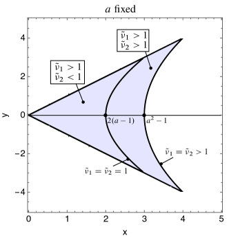
Figure 6: The parameter region representing bipartite Gaussian states in the $(x,y)$ plane (shaded region). The region $(x+2)^{2}-y^{2}<4a^{2}$ corresponds to entangled states and the region $(x+2)^{2}-y^{2}>4a^{2}$ corresponds to separable states.

Symplectic eigenvalues of the four-mode state ABCD are given by

$$\sqrt{(a-d_{1})(a-d_{2})-(g-h)^{2}}=1,\quad\sqrt{(a+d_{1})(a+d_{2})-(g+h)^{2}}=1,$$ (137)

which implies the state ABCD is pure. Symplectic eigenvalues of the partially transposed state with bipartition AB:CD are given by

$$(\tilde{\nu}_{2\pm})^{2} =(a-d_{1})(a-d_{2})+(g-h)^{2}\pm 2|g-h|\sqrt{(a-d_{1})(a-d_{2})}$$

$$=(\sqrt{x-y+1}\pm\sqrt{x-y})^{2},$$ (138)

$$(\tilde{\nu}_{1\pm})^{2} =(a+d_{1})(a+d_{2})+(g+h)^{2}\pm 2|g+h|\sqrt{(a+d_{1})(a+d_{2})}$$

$$=(\sqrt{x+y+1}\pm\sqrt{x+y})^{2}.$$ (139)

Therefore, $\tilde{\nu}_{2\pm}=\nu_{2}\pm\sqrt{\nu_{2}^{2}-1},\tilde{\nu}_{1\pm}=\nu_{1}\pm\sqrt{\nu_{1}^{2}-1}$, and the negativity for the bipartition AB:CD is calculated as

$$N_{\text{AB:CD}} =\frac{1}{2}\left(\nu_{1}+\sqrt{\nu_{1}^{2}-1}\right)\left(\nu_{2}+\sqrt{\nu_{2}^{2}-1}\right)-\frac{1}{2}>0.$$ (140)

IV.2 Monogamy relation for Gaussian states

We examine the monogamy inequality (127) for Gaussian states. For the qubit case treated in [14], as the entanglement measure in this monogamy inequality, $\widetilde{E}(\text{A:B})$ can be the negativity $N_{\text{A:B}}$. $E(\text{AB:CD})$ is a decreasing function of the negativity $N_{\text{AB:CD}}$, and the explicit form of this function is presented in [14]. In the present analysis with Gaussian states, we also adopt negativity as an entanglement measure to show a monogamy inequality.

As we have already presented, negativities $N_{\text{A:B}}$ and $N_{\text{AB:CD}}$ are expressed as functions of $a,x,y$:

$$N_{\text{A:B}}(x,y,a)=\frac{1}{2}\left(\frac{1}{\tilde{\nu}_{2}}-1\right),\quad\tilde{\nu}_{2}^{2}=2a^{2}-x-1-\sqrt{y^{2}-4a^{2}(x-a^{2}+1)},$$ (141)

$$N_{\text{AB:CD}}(x,y)=\frac{1}{2}\left(\sqrt{x+y+1}+\sqrt{x+y}\right)\left(\sqrt{x-y+1}+\sqrt{x-y}\right)-\frac{1}{2}.$$ (142)

To capture qualitative behavior of the monogamy relation between $N_{\text{A:B}}$ and $N_{\text{AB:CD}}$, we randomly generate parameters $x,y$ of bipartite Gaussian states with fixed $a$. The left panel of Fig. 7 shows the distribution of $(N_{\text{AB:CD}},N_{\text{A:B}})$ for randomly generated bipartite Gaussian states. We observe that all bipartite Gaussian states are confined in a region surrounded by lines $N_{\text{A:B}}=g_{1}(N_{\text{AB:CD}}),N_{\text{A:B}}=g_{2}(N_{\text{AB:CD}})$, and $N_{\text{A:B}}=0$, i.e.,

$$\begin{cases}g_{1}(N_{\text{AB:CD}})\leq N_{\text{A:B}}\leq g_{2}(N_{\text{AB:CD}})\quad&\text{for}\quad 0\leq N_{\text{AB:CD}}\leq\alpha,\\ 0\leq N_{\text{A:B}}\leq g_{2}(N_{\text{AB:CD}})\quad&\text{for}\quad\alpha\leq N_{\text{AB:CD}}\leq\beta,\\ N_{\text{A:B}}=0\quad&\text{for}\quad\beta\leq N_{\text{AB:CD}},\end{cases}$$ (143)

where functions $g_{1}$ and $g_{2}$ define the relations between $N_{\text{A:B}}$ and $N_{\text{AB:CD}}$ on $|y|=x$ and $y=0$, respectively. They are monotonically decreasing functions of $N_{\text{AB:CD}}$. The parameters $\alpha$ and $\beta$ are defined by $g_{1}(\alpha)=0$ and $g_{2}(\beta)=0$. When $N_{\text{A:B}}$ attains its maximum for a fixed $a$, $N_{\text{AB:CD}}=0$, and hence, the bipartite state AB is pure. The explicit expression of functions $g_{2}$ and $\beta$ are obtained as

$$g_{2}=\frac{1}{2}\left(-1+\left(a-\sqrt{a^{2}-\frac{(N_{\text{AB:CD}}+1)^{2}}{2N_{\text{AB:CD}}+1}}\right)^{-1}\right),$$ (144)

$$\beta=-\frac{1}{2}+\left(\sqrt{a-1/2}+\sqrt{a-1}\right)^{2}.$$ (145)

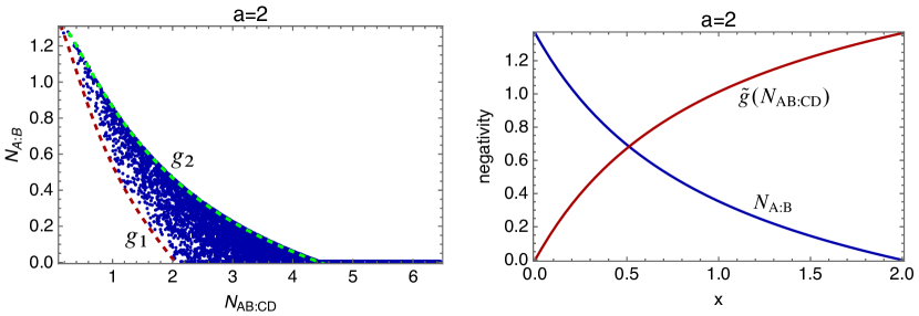
Figure 7: Left panel: distribution of $(N_{\text{AB:CD}},N_{\text{A:B}})$ for randomly generated bipartite Gaussian states with fixed $a$ [11189 sets of parameters $(x,y)$]. States are located in the region surrounded by the dashed green line (corresponds to $y=0$) and the dashed red line (corresponds to $|y|=x$). In this case with $a=2$, for states with $\beta=2+\sqrt{6}<N_{\text{AB:CD}}$, $N_{\text{A:B}}=0$; thus the external correlation between AB and CD limits the amount of the internal entanglement between A and B. The same relation also holds for any values of $a>1$. Right panel: Behavior of $N_{\text{A:B}}$ and $\tilde{g}(N_{\text{AB:CD}})$ as functions of $x$ (with $y=0$). A trade-off relation between the internal entanglement $N_{\text{A:B}}$ and the external entanglement $N_{\text{AB:CD}}$ can be observed. For $\beta=2(a-1)\leq x$, $N_{\text{A:B}}=0$.

For $\alpha\leq N_{\text{AB:CD}}\leq\beta$ with fixed $a$, the following inequality holds:

$$N_{\text{A:B}}\leq g_{2}(N_{\text{AB:CD}},a).$$ (146)

Thus the function $g_{2}$ determines the upper bound of $N_{\text{A:B}}$ for given values of $N_{\text{AB:CD}}$ and $a$. Here, $g_{2}$ is a decreasing function of $N_{\text{AB:CD}}$ and becomes zero at $N_{\text{AB:CD}}=\beta$. We rewrite this inequality as

$$N_{\text{A:B}}+\tilde{g}(N_{\text{AB:CD}},a)\leq N_{\text{A:B}}|_{\text{max}}(a),$$ (147)

where we introduced

$$\tilde{g}(N_{\text{AB:CD}},a):=\begin{cases}0\quad&(N_{\text{AB:CD}}=0)\\ N_{\text{A:B}}|_{\text{max}}(a)-g_{2}(N_{\text{AB:CD}},a)\quad&(0\leq N_{\text{AB:CD}}\leq\beta)\\ N_{\text{A:B}}|_{\text{max}}(a)\quad&(\beta\leq N_{\text{AB:CD}})\end{cases}$$ (148)

and $N_{\text{A:B}}|_{\text{max}}$ is defined by (135). Note that for fixed $a$, $\tilde{g}$ is a non-negative monotonically increasing function of $N_{\text{AB:CD}}$. Furthermore, it vanishes if $N_{\text{AB:CD}}=0$. In this sense, the function $\tilde{g}$ defines an entanglement measure for bipartition AB:CD for each $a$. Thus for Gaussian states with fixed $a$, we have obtained the monogamy inequality (147) that represents a trade-off relation between the internal entanglement $N_{\text{A:B}}$ and the external entanglement $\tilde{g}(N_{\text{AB:CD}},a)$. When $\beta\leq N_{\text{AB:CD}}$, $\tilde{g}(N_{\text{AB:CD}},a)$ attains its maximum, and the negativity between A and B automatically vanishes, i.e., $N_{\text{A:B}}=0$.

The right panel of Fig. 7 shows the behavior of $N_{\text{A:B}}$ and $\tilde{g}(N_{\text{AB:CD}})$ as functions of $x$ when $y=0$. This case corresponds to saturation of the inequality (147) and the following equality holds:

$$N_{\text{A:B}}+\tilde{g}(N_{\text{AB:CD}},a)=N_{\text{A:B}}|_{\text{max}}(a).$$ (149)

IV.3 Monogamy for local modes in the de Sitter universe

For the scalar field in the de Sitter universe, components of the covariance matrix of local Gaussian modes are functions of $a_{\text{sc}}$ and $\delta$. Figure 8 shows the evolution of $N_{\text{A:B}}$ and $N_{\text{AB:CD}}$ with fixed $\delta$. The left panel shows relations between $N_{\text{A:B}}$ and $N_{\text{AB:CD}}$ with different values of $\delta$. The state evolves from $a_{\text{sc}}=0$ that corresponds to the left edges of each line. As we have already observed, $N_{\text{A:B}}$ becomes zero when the physical size $\delta\times a_{\text{sc}}$ of local modes exceeds the Hubble horizon scale $H^{-1}$. On the other hand, $N_{\text{AB:CD}}$ increases monotonically with the scale factor for a fixed value of $\delta$; thus, $N_{\text{A:B}}$ becomes zero as $N_{\text{AB:CD}}$ reaches a some critical value.

The right panel of Fig. 8 shows the evolution of negativities and $\beta$ as functions of the scale factor for $\delta=0.2$. The behavior of $N_{\text{A:B}}$ and $N_{\text{AB:CD}}$ represents a trade-off relation between them. From the argument in the previous subsection, they satisfy the monogamy relation

$$N_{\text{A:B}}+\tilde{g}(N_{\text{AB:CD}},a(a_{\text{sc}},\delta))\leq N_{\text{A:B}}|_{\text{max}}(a(a_{\text{sc}},\delta)).$$ (150)

Note that this inequality is essentially the same as (147), but the parameter $a$ becomes a function of $a_{\text{sc}}$ and $\delta$. It explains the separable behavior of the bipartite system AB as a monogamy relation between internal entanglement and external entanglement; for $\beta(a(a_{\text{sc}},\delta))\leq N_{\text{AB:CD}}$, the function $\tilde{g}$ attains its maxima while $N_{\text{A:B}}$ vanishes. Thus, this inequality provides a sufficient condition of separability for the bipartite system AB. Although $N_{\text{A:B}}$ becomes zero before $N_{\text{AB:CD}}$ reaches $\beta$ (see right panel of Fig. 8), this behavior is consistent with (150). The tightness of the monogamy inequality depends on the parameter $\delta$ in the present setup. Actually, as $\delta$ increases, the difference between $g_{2}(N_{\text{AB:CD}},a(a_{\text{sc}},\delta))$ and $N_{\text{A:B}}$ decreases. In the limit of $\delta\rightarrow 1$ (pure state limit), $N_{\text{A:B}}=g_{2}(N_{\text{AB:CD}},a)$ holds because $N_{\text{A:B}}\rightarrow 0$ and $N_{\text{AB:CD}}\rightarrow 0$, which implies that equality in (150) trivially holds.

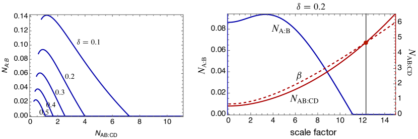
Figure 8: Left panel: relation between $N_{\text{A:B}}$ and $N_{\text{AB:CD}}$ for fixed values of $\delta$. Right panel: evolution of $N_{\text{A:B}}$, $N_{\text{AB:CD}}$ and $\beta$ as functions of the scale factor. The solid red circle denotes the location at $N_{\text{AB:CD}}=\beta$ and the solid black line indicates a value of the scale factor. For the right side of this point, $\beta<N_{\text{AB:CD}}$ and the monogamy inequality (150) implies $N_{\text{A:B}}=0$.

V Summary and conclusion

We investigated the emergence of separability for local bipartite modes assigned to two spatial regions in the de Sitter universe. The bipartite mode AB becomes separable after their separation exceeds the Hubble horizon scale. To understand the emergence of this separability from the viewpoint of entanglement monogamy, we considered purification of the local mode AB and obtained the pure four-mode state ABCD applying the partner formula. Then, we found the monogamy inequality between the negativity $N(\text{A:B})$ and $N(\text{AB:CD})$ for the four-mode Gaussian state, which is an extension of Camalet’s monogamy relation to continuous variable systems. It is demonstrated that the separability of the mode AB can be understood as the monogamy property between the internal and the external entanglements, and the monogamy inequality provides a sufficient condition for the separability of the local mode AB defined from the quantum field. In the stochastic approach to inflation [25], local oscillator modes are defined as long wavelength components of the inflaton field. The introduced local modes are treated as “classical” stochastic variables, and they obey a Langevin equation with a stochastic noise originating from the short wavelength quantum fluctuations. Although the stochastic approach to inflation is a phenomenological treatment of quantum fields in the de Sitter spacetime and is widely employed to investigate the physics related to cosmic inflation, its justification is still missing. Our investigation of this paper provides one reasoning to this method from the viewpoint of quantum information; local modes in the de Sitter universe lose quantum correlation when their separation exceeds the cosmological horizon, and this behavior is related to delocalization of partner modes.

The partner formula adopted in this study may provide a new perspective on information sharing in multipartite quantum systems. Indeed, as shown in Fig. 4, the spatial profiles of partner modes can be visualized and they are helpful in capturing how the information of a system is shared with its partners. The information stored in a system is lost but classical properties of the system appear as a result of decoherence via information sharing with its partners (environments). This direction of investigation is closely related to the concept of “quantum Darwinism” [35] which states that the emergence of a classical behavior of a quantum system, such as objectivity, is connected with the amount of information of the system redundantly shared or stored in the environment. Thus spatial profiles of partner modes of the system may help to quantify this redundancy of the information and to understand the quantum to classical transition in the early universe.

Appendix A CONVENTIONAL MONOGAMY RELATION

We present the conventional monogamy relation for Gaussian states [10, 11, 12]. For the four-mode pure Gaussian state ABCD with the covariance matrix (124),

$$E(\text{A:B})+E(\text{A:C})+E(\text{A:D})\leq E(\text{A:BCD}),$$ (151)

where $E$ denotes a suitably chosen entanglement measure and this inequality holds with the square of negativity or square of logarithmic negativity as entanglement measures. We demonstrate it for randomly generated Gaussian states by taking $E$ as the square of negativity. Negativities are given by

$$N_{\text{A:BCD}}=\frac{1}{2}\left(a+\sqrt{a^{2}-1}-1\right),$$ (152)

$$N_{\text{A:C}}=\mathrm{max}\left[\frac{1}{2a-(\sqrt{x+y}+\sqrt{x-y})}-\frac{1}{2},0\right],$$ (153)

$$N_{\text{A:D}}=\mathrm{max}\left[\frac{1}{2a-(\sqrt{x+y}-\sqrt{x-y})}-\frac{1}{2},0\right],$$ (154)

and $N_{\text{A:B}}$ is given by (133). We can observe the monogamy inequality (151) indeed holds for this four-mode Gaussian state (Fig. 9) because generated states are located below the dashed red lines that represent equality of (151). However, Fig. 9 shows that states deviate from the dashed red lines as the parameter $a$ increases. Therefore, the monogamy inequality (151) does not provide a useful tight constraint on the separability of the bipartite state AB.

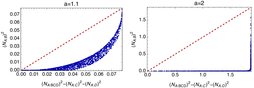
Figure 9: Demonstration of the monogamy inequality (151) for the four-mode Gaussian state with the covariance matrix (124). The number of randomly generated states is 1500. As an entanglement measure, the square of negativity is adopted. All generated states are located below the dashed red line, which represents the equality of the relation (151).

References

- Kiefer and Polarski [2008] C. Kiefer and D. Polarski, Why do cosmological perturbations look classical to us?, Adv. Sci. Lett. 2, 164 (2008) .
- Nambu [2008] Y. Nambu, Entanglement of quantum fluctuations in the inflationary universe, Phys. Rev. D 78, 044023 (2008).
- Nambu and Ohsumi [2009] Y. Nambu and Y. Ohsumi, Entanglement of a coarse grained quantum field in the expanding universe, Phys. Rev. D 80, 124031 (2009).
- Nambu and Ohsumi [2011] Y. Nambu and Y. Ohsumi, Classical and quantum correlations of scalar field in the inflationary universe, Phys. Rev. D 84, 044028 (2011).
- Nambu [2013] Y. Nambu, Entanglement Structure in Expanding Universes, Entropy 15, 1847 (2013).
- Matsumura and Nambu [2018] A. Matsumura and Y. Nambu, Large scale quantum entanglement in de Sitter spacetime, Phys. Rev. D 98, 025004 (2018) .
- Nambu and Hotta [2023] Y. Nambu and M. Hotta, Analog de Sitter universe in quantum Hall systems with an expanding edge, Phys. Rev. D 107, 085002 (2023) .
- Coffman et al. [2000] V. Coffman, J. Kundu, and W. K. Wootters, Distributed entanglement, Phys. Rev. A 61, 052306 (2000).
- Osborne and Verstraete [2006] T. J. Osborne and F. Verstraete, General monogamy inequality for bipartite qubit entanglement, Phys. Rev. Lett. 96, 1 (2006) .
- Hiroshima et al. [2007] T. Hiroshima, G. Adesso, and F. Illuminati, Monogamy Inequality for Distributed Gaussian Entanglement, Phys. Rev. Lett. 98, 050503 (2007) .
- Adesso and Illuminati [2007] G. Adesso and F. Illuminati, Strong Monogamy of Bipartite and Genuine Multipartite Entanglement: The Gaussian Case, Phys. Rev. Lett. 99, 150501 (2007).
- Adesso et al. [2014] G. Adesso, S. Ragy, and A. R. Lee, Continuous Variable Quantum Information: Gaussian States and Beyond, Open Systems and Information Dynamics 21, 1440001 (2014).
- Dhar et al. [2016] H. S. Dhar, A. K. Pal, D. Rakshit, A. S. De, and U. Sen, Monogamy of quantum correlations - a review, in Lectures on General Quantum Correlations and their Applications (Springer, Cham, 2017) .
- Camalet [2017a] S. Camalet, Monogamy Inequality for Any Local Quantum Resource and Entanglement, Phys. Rev. Lett. 119, 110503 (2017a).
- Camalet [2017b] S. Camalet, Monogamy inequality for entanglement and local contextuality, Phys. Rev. A 95, 062329 (2017b).
- Camalet [2018] S. Camalet, Internal Entanglement and External Correlations of Any Form Limit Each Other, Phys. Rev. Lett. 121, 60504 (2018).
- Zhu et al. [2020] J. Zhu, M.-J. Hu, Y. Dai, Y.-K. Bai, S. Camalet, C. Zhang, C.-F. Li, G.-C. Guo, and Y.-S. Zhang, Realization of the tradeoff between internal and external entanglement, Phys. Rev. Res. 2, 043068 (2020) .
- Zhu et al. [2021] J. Zhu, Y. Dai, S. Camalet, C.-J. Zhang, B.-H. Liu, Y.-S. Zhang, C.-F. Li, and G.-C. Guo, Observation of the tradeoff between internal quantum nonseparability and external classical correlations, Phys. Rev. A 104, 062442 (2021) .
- Trevison et al. [2019] J. Trevison, K. Yamaguchi, and M. Hotta, Spatially overlapped partners in quantum field theory, J. Phys. A Math. Theor. 52, (2019).
- Tomitsuka et al. [2019] T. Tomitsuka, K. Yamaguchi, and M. Hotta, Partner formula for an arbitrary moving mirror in $1+1$ dimensions, Phys. Rev. D 101, 24003 (2019) .
- Yamaguchi [2020] K. Yamaguchi, PhD Thesis: Quantum Information Capsule and Its Applications to Communication Through Quantum Fields, Ph.D. thesis, Tohoku University (2020).
- Yamaguchi and Hotta [2020] K. Yamaguchi and M. Hotta, Quantum information capsule in multiple-qudit systems and continuous-variable systems, Phys. Lett. A 384, 126447 (2020).
- Yamaguchi et al. [2020] K. Yamaguchi, A. Ahmadzadegan, P. Simidzija, A. Kempf, and E. Martín-Martínez, Superadditivity of channel capacity through quantum fields, Phys. Rev. D 101, 105009 (2020).
- Birrell and Davies [1984] N. D. Birrell and P. C. W. Davies, Quantum fields in curved space (Cambridge University Press, 1984).
- Starobinsky [1988] A. A. Starobinsky, Stochastic de sitter (inflationary) stage in the early universe, in F. Theory, Quantum Gravity Strings (1988) pp. 107–126.
- Peres [1996] A. Peres, Separability Criterion for Density Matrices, Phys. Rev. Lett. 77, 1413 (1996) .
- Horodecki [1997] P. Horodecki, Separability criterion and inseparable mixed states with positive partial transposition, Phys. Lett. A 232, 333 (1997) .
- Simon [2000] R. Simon, Peres-Horodecki Separability Criterion for Continuous Variable Systems, Phys. Rev. Lett. 84, 2726 (2000).
- Vidal and Werner [2002] G. Vidal and R. Werner, Computable measure of entanglement, Phys. Rev. A 65, 032314 (2002).
- Plenio [2005] M. Plenio, Logarithmic Negativity: A Full Entanglement Monotone That is not Convex, Phys. Rev. Lett. 95, 090503 (2005).
- Hotta et al. [2015] M. Hotta, R. Schützhold, and W. G. Unruh, Partner particles for moving mirror radiation and black hole evaporation, Phys. Rev. D 91, 124060 (2015) .
- Yamaguchi et al. [2019] K. Yamaguchi, N. Watamura, and M. Hotta, Quantum information capsule and information delocalization by entanglement in multiple-qubit systems, Phys. Lett. A 383, 1255 (2019) .
- Duan et al. [2000] L. Duan, G. Giedke, J. Cirac, and P. Zoller, Inseparability criterion for continuous variable systems, Phys. Rev. Lett. 84, 2722 (2000).
- Serafini and Adesso [2007] A. Serafini and G. Adesso, Standard forms and entanglement engineering of multimode Gaussian states under local operations, J. Phys. A Math. Theor. 40, 8041 (2007) .
- Zurek [2009] W. H. Zurek, Quantum Darwinism, Nat. Phys. 5, 181 (2009).