Representation of Lexical Stylistic Features
in Language Models’ Embedding Space

Abstract

The representation space of pretrained Language Models (LMs) encodes rich information about words and their relationships (e.g., similarity, hypernymy, polysemy) as well as abstract semantic notions (e.g., intensity). In this paper, we demonstrate that lexical stylistic notions such as complexity, formality, and figurativeness, can also be identified in this space. We show that it is possible to derive a vector representation for each of these stylistic notions from only a small number of seed pairs. Using these vectors, we can characterize new texts in terms of these dimensions by performing simple calculations in the corresponding embedding space. We conduct experiments on five datasets and find that static embeddings encode these features more accurately at the level of words and phrases, whereas contextualized LMs perform better on sentences. The lower performance of contextualized representations at the word level is partially attributable to the anisotropy of their vector space, which can be corrected to some extent using techniques like standardization.

1 Introduction

The style of a text is often reflected in its grammatical and discourse properties, but also in local word choices made by the author. The choice of one from a set of synonyms or paraphrases with different connotations can define the style of a text in terms of complexity (e.g., help vs. assist), formality (e.g., dad vs. father), figurativeness (e.g., fall vs. plummet), and so on (Edmonds and Hirst, 2002). These lexical stylistic features can be useful in various scenarios, such as analyzing the style of authors or texts of different genres, and determining the appropriate word usage in language learning applications.

Complexity	doctor $\rightarrow$ medical practitioner
	laws $\rightarrow$ legislative texts
	high blood pressure $\rightarrow$ hypertension
	very common $\rightarrow$ prevalent
	a lot $\rightarrow$ significant quantity
	be bad $\rightarrow$ impact negatively
	help $\rightarrow$ assist
Formality	my gosh $\rightarrow$ jesus
	breathing $\rightarrow$ respiratory
	yeah $\rightarrow$ yes
	ten years $\rightarrow$ decade
	first of all $\rightarrow$ foremost
	a whole bunch $\rightarrow$ full
	my dad $\rightarrow$ father
Figurativeness	bright $\rightarrow$ radiant
	heavy $\rightarrow$ burdened
	unsympathetic $\rightarrow$ cold-hearted
	fall $\rightarrow$ plummet
	a lot of $\rightarrow$ a sea of
	quick $\rightarrow$ lightning
	hard $\rightarrow$ ironclad

Table 1: Seed pairs for constructing vector representations of complexity (simple $\rightarrow$ complex), formality (casual $\rightarrow$ formal), and figurativeness (literal $\rightarrow$ figurative).

Previous approaches to formality detection relied on word length, frequency, as well as on the presence of specific prefixes and suffixes (e.g., intra-, -ation) Brooke et al. (2010). Such features have also been used for complexity detection, often combined with information regarding the number of word senses and synonyms Shardlow (2013); Kriz et al. (2018). Recent studies have shown that the representation space of pretrained LMs encodes a wealth of lexical semantic information, including similarity, polysemy, and hypernymy (Garí Soler and Apidianaki, 2021a; Pimentel et al., 2020; Ettinger, 2020; Ravichander et al., 2020; Vulić et al., 2020, i.a.). In particular, abstract semantic notions such as intensity (e.g., pretty $\rightarrow$ beautiful $\rightarrow$ gorgeous) can be extracted using a lightweight approach based on simple calculations in the vector space Garí Soler and Apidianaki (2020, 2021b).

In this paper, we explore whether lexical stylistic features can also be identified in the vector space built by pretrained LMs. To do this, we extend the method of Garí Soler and Apidianaki (2020) to address complexity, formality, and figurativeness. We first construct a vector representation for each of these features using a small number of seed pairs shown in Table 1. We then use these vectors to characterize new texts according to these stylistic dimensions, by applying simple calculations in the vector space. We evaluate our method using a binary classification task: given a pair of texts that are semantically similar but stylistically different in terms of some target feature (e.g., formality), the task is to determine which text exhibits the feature more strongly (e.g., is more formal). Note that the goal of our study is not to achieve high performance on the task itself, but rather to probe for how well these stylistic features are encoded in different types of pretrained representations.

We experiment with various static and contextualized embeddings on five datasets, containing words and phrases (doctor vs. medical practitioner), or sentences (Those recommendations were unsolicited and undesirable. vs. that’s the stupidest suggestion EVER.). Our results show that both types of representations can capture these stylistic features reasonably well, although static embeddings perform better at the word and phrase level, and contextualized LMs at the sentence level. We hypothesize that the sub-optimal performance of contextualized LMs on short texts might be partially due to the high anisotropy of their embedding space. Anisotropic word representations occupy a narrow cone instead of being uniformly distributed in the vector space, resulting in highly positive correlations even for unrelated words, thus negatively impacting the quality of the similarity estimates that can be drawn from the space Ethayarajh (2019); Gao et al. (2019); Cai et al. (2021); Rajaee and Pilehvar (2021). We verify this hypothesis by implementing different anisotropy correction strategies (Timkey and van Schijndel, 2021) and discuss the observed improvements in contextualized representations’ performance on short texts.

Overall, our findings contribute to the big picture of probing literature, showing that stylistic features like complexity, formality, and figurativeness can be decoded from the embedding space of pretrained representations using simple calculations, without any supervision. Our lightweight method can be easily integrated into downstream applications like authorship attribution and style transfer.

2 Related work

There has been an extensive body of literature on probing techniques aimed at identifying the linguistic and world knowledge encoded in LM representations. For example, given a Machine Translation model, does it implicitly capture the syntax structure of the source text? Existing work addresses such questions with methods like auxiliary classifiers (a.k.a. probing/diagnostic classifiers) Veldhoen et al. (2016); Adi et al. (2017); Conneau et al. (2018), information-theoretic probing Voita and Titov (2020); Lovering et al. (2020), behavioral tests Ebrahimi et al. (2018); Wallace et al. (2019); Petroni et al. (2019), geometric probing Chang et al. (2022); Wartena (2022); Kozlowski et al. (2019), visualization of model-internal structures Raganato and Tiedemann (2018), and so on. Using these methods, researchers have found that pretrained LMs do encode various types of knowledge, including syntactic Linzen et al. (2016); Hewitt and Manning (2019), semantic Ettinger et al. (2016); Adi et al. (2017); Yanaka et al. (2020), pragmatic Jeretic et al. (2020); Schuster et al. (2020), as well as factual and commonsense knowledge Petroni et al. (2019); Thukral et al. (2021).

Our work is along the line of probing for lexical semantics with simple geometry-based methods Vulić et al. (2020); Garí Soler and Apidianaki (2021a), which uncovers the target knowledge encoded in the semantic space of LM representations with simple geometric computations Vulić et al. (2020); Garí Soler and Apidianaki (2021a). Compared to the most widely used auxiliary classifier method, geometric probing does not rely on any external model. Thus, it requires no annotated training data and avoids the potential issue of the external model itself learning the target knowledge Hewitt and Liang (2019).

Directly related to our work, Garí Soler and Apidianaki (2020) proposed a method to detect the intensity of scalar adjectives, where an “intensity” dimension is identified in the vector space built by the BERT model. The method draws inspiration from word analogies in gender bias work, where a gender subspace is identified in the embedding space by calculating the main direction spanned by the differences between vectors of gendered word pairs (e.g., $\overrightarrow{he}$ - $\overrightarrow{she}$, $\overrightarrow{man}$ - $\overrightarrow{woman}$) Bolukbasi et al. (2016); Dev and Phillips (2019). Similarly, Garí Soler and Apidianaki (2020) view intensity as a direction in the embedding space which is calculated by subtracting the vector of a low-intensity adjective from that of a high-intensity adjective on the same scale (e.g., $\overrightarrow{awesome}$ - $\overrightarrow{good}$, $\overrightarrow{horrible}$ - $\overrightarrow{bad}$). Intuitively, this subtraction cancels out the adjectives’ common denotation and retains their variance in intensity, which is represented by the resulting difference vector ($\overrightarrow{dVec}$). This vector can then be used to determine the intensity of new adjectives by simply taking the cosine similarity of their vector to $\overrightarrow{dVec}$. We extend this method to other lexical stylistic notions, and address words of different part-of-speech (POS) and longer texts.

3 Method

Figure 1: Complexity vector generation.

We adopt the definitions for the three stylistic features of interest (complexity, formality, and figurativeness) proposed by previous work. Simple language is “used to talk to children or non-native English speakers”, whereas more complex language is “used by academics or domain experts” Pavlick and Nenkova (2015). Formal language is defined as “the way one talks to a superior”, whereas casual language is “used with friends” Pavlick and Nenkova (2015). Figurative language is defined by Stowe et al. (2022) as utterances “in which the intended meaning differs from the literal compositional meaning”, while literal language exhibits no such difference. Unlike the previous two features, figurativeness is often a contextual instead of lexical feature (e.g., the word adhere is used in a metaphorical sense in the expression “adhere to the rules” and in its literal sense in “adhere to the wall”). We explore the usability of our method for studying figurativeness by using a small seed set of synonyms and paraphrases that have literal and figurative connotations (e.g., unsympathetic $\rightarrow$ cold-hearted) independent of their context. These pairs are only used for constructing our figurativeness vector representation, while our evaluation is performed on a dataset containing full sentences (see Section 4 for details).

Our method involves two steps: (a) feature vector generation, where we construct a vector representation for each feature; and (b) feature value prediction, where we predict how strongly a new piece of text exhibits some target feature using the constructed feature vector. We illustrate the two steps below.

Feature vector generation.

We collect a small number of seed pairs to illustrate each notion, shown in Table 1. The seed pairs consist of rough paraphrases that differ in the stylistic aspect of interest. Consider complexity as an example. Given a pair of “simple $\rightarrow$ complex” texts, we subtract the vector of the simple from that of the complex one (e.g., $\overrightarrow{medical\;practitioner}$ - $\overrightarrow{doctor}$). After performing this subtraction for each pair in the seed set, we then average the resulting difference vectors to obtain a vector representing complexity which we call $\overrightarrow{d_{complex}}$. This procedure is illustrated in Figure 1. Similarly, for formality, we subtract the vector of the informal paraphrase from that of its formal counterpart (e.g., $\overrightarrow{respiratory}$ - $\overrightarrow{breathing}$), and for figurativeness, we subtract the vector of the literal expression from that with figurative meaning (e.g., $\overrightarrow{bright}$ - $\overrightarrow{radiant}$). By averaging the difference vectors for all pairs in the corresponding seed set, we obtain vectors representing formality ($\overrightarrow{d_{formal}}$) and figurativeness ($\overrightarrow{d_{fig}}$). We extend the method of Garí Soler and Apidianaki (2020), which was only applied to scalar adjectives, to words of other POS and to longer text (phrases and sentences). Finally, we compare the vectors that are built using representations from different monolingual and multilingual models.

Feature value prediction.

Given a new piece of text (word, phrase, or sentence), we compute the cosine similarity between its vector representation and $\overrightarrow{d_{complex}}$, $\overrightarrow{d_{formal}}$ and $\overrightarrow{d_{fig}}$. The more similar the vector of the new text is to one of these feature vectors, the more complex, formal, or figurative the text is considered to be.

4 Experimental Setup

Evaluation task and metrics. We evaluate the representation of the target features in a binary classification task: given a pair of texts (words, phrases, or sentences) $t_{0}$ and $t_{1}$ that are semantically similar but stylistically different in terms of some feature $F$ (e.g., figurativeness), the task is to decide which text exhibits the feature more strongly (e.g., is more figurative). For example, given two sentences “You must adhere to the rules.” ($t_{0}$) and “You must obey the rules.” ($t_{1}$), the ground truth is that $t_{0}$ is more figurative. We use accuracy as our evaluation metric.

Seed pairs. For each feature, we use seven seed pairs for vector generation, as shown in Table 1. The seeds for complexity are examples from the paper describing SimplePPDB Pavlick and Callison-Burch (2016), and the seeds for formality are from the paper on lexical style properties of paraphrases Pavlick and Nenkova (2015). For figurativeness, we manually compile a set of seven seed pairs.

Feature	Short-text (word/phrase)	Long-text (sentence)
Complexity	SimplePPDB	SimpleWikipedia
Formality	StylePPDB	GYAFC
Figurativeness	–	IMPLI

Table 2: Datasets used for each feature.

Datasets. The datasets used in our feature value prediction experiments (described in Table 2) contain pairs of words or phrases (short text), and pairs of sentences (long text). Note that this distinction is not based on the number of tokens, but on whether the text is a complete sentence. For complexity, we use SimplePPDB Pavlick and Callison-Burch (2016) and SimpleWikipedia Kauchak (2013); for formality, Style-annotated PPDB (StylePPDB for short) Pavlick and Nenkova (2015) and GYAFC Rao and Tetreault (2018). For figurativeness, since there is no dataset of word and/or phrase pairs, we only use the IMPLI (Idiomatic and Metaphoric Paired Language Inference) dataset Stowe et al. (2022) that contains sentences.

For each dataset, we select the optimal configuration (see the Configuration paragraph below) using the validation set, and report its performance on the test set. To make the label distribution balanced, we randomly shuffle the order of the two pieces of text in each pair and re-assign the gold label accordingly. This ensures that a majority baseline only performs around chance. Figure 2 shows the distribution of token frequency in each dataset.

Figure 2: Distribution of token frequency in the evaluation datasets.

Baselines. We compare our method to two simple baselines. The majority baseline always predicts the majority label in the dataset. The frequency baseline consults the frequency counts of each token in the Google N-gram corpus Brants (2006) and considers more frequent tokens to be simpler, more casual, and more literal. Frequency has been a strong baseline for complexity and formality in previous work, given that rare words tend to be more complex than frequently used words Brooke et al. (2010).

Pooling	Model	Complexity		Formality		Figurativeness
		short	long	short	long	long
	majority	55.1	50.6	51.2	51.8	51.4
Mean	frequency	83.2	51.0	61.0	41.4	49.7
2-7	static	84.8 glove	60.0 glove	76.8 glove	82.8 glove	54.3 glove
2-7	contextualized (single layer)	86.2 roberta-large (4)	76.5 mbert-base (1)	68.7 bert-base (1)	82.4 roberta-large (12)	72.9 bert-large (14)
2-7	contextualized (layer agg)	84.4 mbert-base (10)	76.0 mbert-base (11)	67.6 bert-large (1)	86.7 roberta-large (23)	67.2 bert-large (19)
Max	frequency	80.7	46.4	57.2	42.5	47.9
2-7	static	89.4 glove	58.0 glove	76.0 glove	63.4 glove	56.0 fasttext
2-7	contextualized (single layer)	87.7 roberta-large (4)	69.4 roberta-base (12)	71.7 mbert-base (0)	73.6 mbert-base (1)	64.8 bert-large (11)
2-7	contextualized (layeragg)	86.2 roberta-large (19)	67.6 roberta-large (4)	71.7 mbert-base (0)	71.7 roberta-large (24)	63.9 bert-large (14)

Table 3: Accuracy scores obtained on each test set using different types of embeddings and pooling methods. We report the performance of the models and layers (in parentheses) that best predicted the feature on the corresponding validation set. For contextualized representations, we report results using a single layer or layer aggregation (“layer agg”). The highest performance obtained with each pooling method (Mean/Max) is in boldface.

Pooling	Stats	Complexity		Formality		Figurativeness
		short	long	short	long	long
Mean	2 beats 1 (%)	63.0	78.0	92.9	72.4	54.3
	acc gain	2.6	4.1	4.3	5.3	0.1
Max	2 beats 1 (%)	66.1	72.4	95.3	64.6	44.9
	acc gain	3.0	3.0	4.4	3.2	-0.5
Average	2 beats 1 (%)	64.6	75.2	94.1	68.5	49.6
	acc gain	2.8	3.5	4.3	4.3	-0.2

Table 4: Comparison between single layer and layer aggregation settings. “2 beats 1 (%)” refers to the percentage of cases where layer aggregation performance is at least as high as the single layer performance, under the same configuration (LM & layer). “Acc gain” stands for the average accuracy gain of layer aggregation over single layer across all configurations. Positive accuracy gains are highlighted in green, negative ones in pink.

Configuration. We experiment with two parameters in the configuration: LM and layer. Note that the purpose of experimenting with different configurations is not to solve the task, but rather to obtain a comprehensive picture of which embeddings best represent the target features.

• Language Models: We experiment with both static and contextualized representations. For static embeddings, we consider GloVe Pennington et al. (2014) and fastText Bojanowski et al. (2017). For contextualized LMs, we consider encoder-only monolingual and multilingual Transformer models of different sizes (base and large), including BERT Devlin et al. (2019), mBERT (multilingual BERT) Devlin et al. (2019), RoBERTa Liu et al. (2019), and XLM-RoBERTa Conneau et al. (2020).

• Layer ($l$): For contextualized LMs, another configuration choice is which layer to obtain the representation from. We explore the knowledge encoded in different layers in the range of 0-12 for base models and 0-24 for large ones, including the embedding layer.

Pooling strategies. In order to obtain a score for a feature of interest (complexity, formality, or figurativeness) for text segments that contain more than one token (i.e., phrases and sentences), we consider two pooling strategies over the scores calculated for individual tokens:

• mean: We compute the cosine similarity between $\overrightarrow{d_{feature}}$ and each word vector, and take the average of the similarity scores as the feature value for the text.

• max: We compute the cosine similarity between $\overrightarrow{d_{feature}}$ and each word vector, and take the maximum of the similarity scores as the feature value for the text.

The intuition behind max pooling is that the majority of words in a phrase or sentence would not be too extreme (i.e., too complex or too formal). By looking at the most complex or formal word in the text, we can get an idea of how extreme it might be in that dimension. Naturally, we expect this approach to perform less well than mean pooling for figurativeness, where idiomaticity is most often inferred by looking at the context of use and the word combinations within a sentence.

5 Results and Discussion

Table 3 presents the results of our evaluation. Due to space constraints, each row in the table only shows the optimal performance obtained across all configurations (LM and layers) for static and contextualized models. For contextualized LMs in particular, following Vulić et al. (2020), we separately show the optimal performance under two settings: single layer, where only the representation from a single layer $l$ is used; and layer aggregation (“layeragg” for short), where we average the representations from all layers from the 0th to a specific layer $l$ (included).

(a) Complexity (short)

(b) Formality (short)

(c) Complexity (long)

(d) Formality (long)

(e) Figurativeness (long)

Figure 3: Performance change across layers of different LMs (under the layer aggregation setting).

We observe that our method outperforms the majority and frequency baselines with both static and contextualized LMs. Furthermore, mean pooling generally works better than max pooling, although there is still room for improvement. Taking a closer look at the optimal configuration for each feature, for complexity, roberta-large and mbert-base are the dominant best-performing models, yet there are no consistently dominant layers; for formality, bert-base and mbert-base perform the best on short texts and surprisingly with the initial layers (0 or 1), while roberta-large is the best model for long texts with middle or final layers; for figurativeness, bert-large is consistently the best model across all settings.

Interestingly, contextualized LMs far outperform static embeddings on long text sin almost all cases, yet on short texts, static embeddings perform on par or sometimes even better than contextualized LMs. This is the case, for example, with formality “short” (with both pooling strategies) and with complexity “short” (with max pooling). This finding sounds counter-intuitive, given the generally higher performance of contextualized models in various NLP tasks. In our probing setting, we suspect that this might be due to two factors. First, the input in short-text datasets consists of isolated, rather than contextualized, instances of words. This is not natural input for a contextualized LM. Second, previous work has demonstrated that the word-level similarity estimates obtained from the vector space of contextualized LMs might be distorted due to the anisotropy of the space Ethayarajh (2019); Rajaee and Pilehvar (2021). Concretely, anisotropic word representations occupy a narrow cone instead of being uniformly distributed in the vector space, resulting in excessively positive correlations even for unrelated word instances. This has a negative impact on the informativeness of measures such as the cosine and the Euclidean distance, often used for estimating representation similarity Apidianaki (2023). These measures are dominated by a small subset of “rogue dimensions” which drive anisotropy and the drop in representational quality in later layers of the models (Timkey and van Schijndel, 2021). In Section 6, we investigate more closely the impact of anisotropy on our results through a series of experiments involving different anisotropy reduction methods.

(a) Complexity

(b) Formality

(c) Figurativeness

Figure 4: Optimal performance over different bins of text length (under the layer aggregation setting).

Finally, comparing the single layer and layer aggregation settings, their respective optimal configurations result in mostly similar performance across datasets, as shown in Table 3. In order to better understand their difference across all possible LM and layer configurations, we present in Table 4 two types of averaged statistics: the percentage of configurations where the layer aggregation performance is equal or higher than the single layer performance, as well as the average gain in terms of accuracy. We observe that layer aggregation improves the performance for complexity and formality (across 64.6% to 94.1% of the configurations and by an accuracy gain of 2.8 to 4.3), but makes almost no difference for figurativeness. Together with the results from Table 3, this suggests that although layer aggregation does not help with the best configuration, it is beneficial to most configurations on average.

In the next two subsections, we analyze the influence of two more factors on our method: layer depth and text length. For conciseness, we only report the results for the layer aggregation setting. Results for the single layer setting are given in Appendix C.

5.1 How well do different layers represent the target features?

We explore the representation of the three stylistic features inside contextualized LMs by specifically monitoring the change in accuracy observed across layers. The results are shown in Figure 3. The solid curves show results obtained using mean pooling, while the dashed ones correspond to max pooling.

We observe that information about complexity (3(a) and 3(c)) is more clearly and consistently encoded after layer 4 of the models, independent of their size (base or large). Across all layers, mean and max pooling exhibit mostly similar behavior for short texts, while mean pooling is clearly better for longer texts. The pattern for figurativeness is similar (3(e)), though with slightly more fluctuations. For formality, we see a different trend. As shown in Figure 3(b), this feature is encoded more clearly in the early layers of the models for short texts. For longer texts, we see diverging patterns across layers of different models (3(d)). In particular, roberta-large encodes formality better than other tested models while its multilingual versions (xlm-roberta-base and xlm-roberta-large) give much lower results.

5.2 How does text length influence our method?

We analyze the performance change with regard to text length, represented by the average number of tokens in the two texts in a pair. For each feature, we merge examples from the short-text and long-text datasets (if available) and take the predictions from the best-performing contextualized configuration from Table 3. Based on the number of tokens, we group all examples into several bins (unigram, bigram, 3-4, 5-9, 10-14, 15-19, >20) and compute the average accuracy in each bin. Figure 4 shows the results.

Interestingly, we observe different patterns for the three features. For complexity, accuracy scores for shorter texts (0.86 to 0.9) are generally higher than those for long texts (0.73 to 0.77). The drop from 3-4 tokens to 5-9 tokens is particularly clear. For formality, on the contrary, longer texts (0.84 to 0.93) tend to be easier than short ones (0.71 to 0.72). For figurativeness, we do not have results for short texts since no such datasets are available. Within full sentences, we observe that our method works better for shorter sentences (with <5 tokens) than for longer ones (with >=5 tokens) by an accuracy difference of 0.13 to 0.25. One caveat is that these differences are not only influenced by text length, but also by the intrinsic data distribution in different datasets. For example, the domain of the source texts in SimplePPDB (news, legal documents, and movie subtitles) is different from that in SimpleWikipedia (encyclopedia articles). Thus, the accuracy differences could be a result of both factors — text length and text domain.

6 Anisotropy Reduction Experiments

Pooling	Model	Complexity		Formality		Figurativeness
		short	long	short	long	long
Mean	static	84.8	60.0	76.8	82.8	54.3
	contextualized (singlelayer)	86.2	76.5	68.7	82.4	72.9
	contextualized (singlelayer+abtt)	80.3	69.3	76.6	76.7	70.9
	contextualized (singlelayer+standardization)	90.4	73.9	74.1	80.6	68.3
	contextualized (singlelayer+rank)	85.6	76.0	70.8	81.7	71.8
	contextualized (layeragg)	84.4	76.0	67.6	86.7	67.2
	contextualized (layeragg+abtt)	81.7	68.5	76.6	63.0	72.6
	contextualized (layeragg+standardization)	90.4	73.6	75.2	79.9	67.6
	contextualized (layeragg+rank)	83.7	75.7	68.1	82.1	67.0
Max	static	89.4	58.0	76.0	63.4	56.0
	contextualized (singlelayer)	87.7	69.4	71.7	73.6	64.8
	contextualized (singlelayer+abtt)	80.6	64.9	78.2	80.8	66.7
	contextualized (singlelayer+standardization)	90.5	63.8	80.9	81.7	60.4
	contextualized (singlelayer+rank)	87.1	69.6	70.3	76.0	66.5
	contextualized (layeragg)	86.2	67.6	71.7	71.7	63.9
	contextualized (layeragg+abtt)	81.9	63.9	78.2	72.5	71.1
	contextualized (layeragg+standardization)	90.5	63.7	80.9	80.6	61.9
	contextualized (layeragg+rank)	86.1	69.3	71.7	71.5	67.4

Table 5: Performance of three anisotropy reduction methods (all-but-the-top/standardization/rank-based). The highest performance within each pooling method (Mean/Max) is in boldface.

As explained in the previous section, the anisotropy of contextualized LMs’ representation space degrades the quality of the similarity estimates that can be drawn from it Ethayarajh (2019). To see if this has an impact on our method, we apply three post-processing anisotropy reduction methods discussed by Timkey and van Schijndel (2021), which can be used to correct for rogue dimensions and reveal underlying representational quality.

We apply each of these methods to our feature vector construction and feature value prediction processes. Given that our stylistic characterization of new text relies on similarity measurement, we expect that a space that allows us to draw higher-quality similarity estimates would better represent these stylistic features and would also improve feature value prediction. The three methods used in our experiments are:

All-but-the-top (abtt). The method was initially proposed for static embeddings by Mu and Viswanath (2018). The main idea is to subtract the common mean vector and eliminate the top few principal components (PCs) (we use the top $\frac{d}{100}$, where $d$ represents the dimensionality of the vector space, following their suggestion). These subtracted vectors should capture the variance of the rogue dimensions in the model and make the space more isotropic. In Timkey and van Schijndel (2021), the mean vector and PCs are computed from vector representations for an entire corpus. Since our method is unsupervised, we do not assume access to any large corpus and instead compute them based only on the seed pairs (i.e., 14 words and phrases for each feature). Thus, our method still remains lightweight and computationally efficient. It is, however, important to note that this is a local correction (rather than a global one) since we are just using a small number of words and phrases, as in Rajaee and Pilehvar (2021).

Formally, given a set of seed texts of size $|\mathcal{S}|$ (here $|\mathcal{S}|=14$) containing token representations $x\in\mathbb{R}^{d}$, we compute the mean vector $\mu\in\mathbb{R}^{d}$

$$\mu=\frac{1}{|\mathcal{S}|}\cdot\sum_{x\in\mathcal{S}}x$$ (1)

as well as the PCs

$$u_{1},...,u_{d}={\rm PCA}(\{x-\mu,x\in\mathcal{S}\}).$$ (2)

Then, the new representation $x_{abtt}$ for an unseen word vector $x$ is the result of eliminating the mean vector and the top $k$ PCs (here $k=\frac{d}{100}$):

$$x_{abtt}=x-\mu-\sum_{i=1}^{k}\left(u_{i}^{\top}x\right)u_{i}.\\$$ (3)

Standardization. Based on a similar observation as abtt (a non-zero common mean vector and a few dominant directions), another way for adjustment is to subtract the mean vector and divide each dimension by its standard deviation (std), such that each dimension has $\mu_{i}=0$ and $\sigma_{i}=1$. Similarly to abtt, we compute the mean vector and standard deviation using only the seed pairs for each feature.

Formally, we compute the same mean vector $\mu$ as in Equation 1, as well as the standard deviation in each dimension $\sigma\in\mathbb{R}^{d}$

$$\sigma=\sqrt{\frac{1}{|\mathcal{S}|}\cdot\sum_{x\in\mathcal{S}}(x-\mu)^{2}}$$ (4)

The new representation $x_{standard}$ for an unseen word vector $x$ becomes

$$x_{standard}=\frac{x-\mu}{\sigma}.$$ (5)

Rank-based. This method treats a word vector as $d$ observations from an $|\mathcal{S}|$-variate distribution and uses correlation metrics as a measure of similarity, instead of cosine similarity Zhelezniak et al. (2019). Specifically, Spearman’s $\rho$, a non-parametric correlation measure, only considers the ranks of embeddings rather than their values. Thus, it will not be dominated by the rogue dimensions of contextualized LMs. Unlike the previous two methods, this method does not require any computation over the seed pair texts. Formally, given a word vector $x$, the new representation $x_{rank}$ is simply

$$x_{rank}=rank(x).\vspace{-0.2in}$$ (6)

Table 5 shows the effect of applying the three anisotropy reduction strategies under the single layer and layer aggregation settings. Overall, after anisotropy reduction, contextualized LMs outperform static embeddings in all cases except formality “short”, confirming our initial hypothesis. Nevertheless, there is no universally optimal strategy, although standardization works best most of the time. Comparing the two pooling strategies, we find that anisotropy correction helps more often with max pooling than with mean pooling.

It is important to reemphasize that our anisotropy correction approach is local, since it only considers a small set of words and phrases for calculating the mean vector, standard deviation, and PCs. This might be the reason for the relatively small observed effect of these correction procedures in our experiments. In future work, we plan to experiment with a larger corpus, and consequently use a larger part of the vector space for calculating the mean/std/PC vectors, in order to investigate the impact of the quantity of data on the induced similarity estimates.

7 Conclusion

We have shown that the embedding space of pretrained LMs encodes abstract stylistic notions such as formality, complexity, and figurativeness. Using a geometry-based method, we construct a vector representation for each of these features, which can be used to characterize new texts. We find that these notions are present in the space of both static and contextualized representations, and that static embeddings are better at capturing the style of short texts (words and phrases) whereas contextual embeddings at longer texts (sentences). By correcting the anisotropy of contextualized LMs’ representation space, we show that it is possible to close the performance gap from static embeddings on short texts.

Our unsupervised and lightweight method is expected to be applicable for stylistic analysis in other languages and for other stylistic notions, such as concreteness, sentiment, and political stance, which we plan to address in future work. Furthermore, we plan to experiment with anisotropy correction methods on a larger corpus, and to adapt the method for style prediction on longer text (e.g., whole documents). The stylistic measurements obtained using this method can be useful in the creation of lexical style lexicons as well as in downstream applications, for authorship attribution and style transfer.

Limitations

We acknowledge the following limitations of our work: (a) The scope of our experiments is limited to the English language currently. Our method is only evaluated on the level of words, phrases, and sentences, but not at the document level. (b) The effect of anisotropy reduction strategies is shown to be rather mixed. Further investigation is required to determine under what conditions these strategies can prove beneficial in the specific context of stylistic feature extraction. (c) Our work addresses only lexical-level stylistic features and not more global aspects of writing style, such as the diversity of word choice and the utilization of unique syntactic structures. Whether this method can be extended to capture the comprehensive nuances of writing style is an interesting direction for future work.

Ethical Considerations

In this paper, our method is only tested in intrinsic evaluation settings where existing publicly available datasets have been used. It is not integrated into any downstream application, although this type of stylistic analysis could be potentially useful in different settings.

Appendix A Dataset Details

All evaluation datasets we use contain semantically similar but stylistically different words, phrases, or sentences.

A.1 Data Description and Source

Complexity

• SimplePPDB Pavlick and Callison-Burch (2016): It contains 4.5M pairs of words and short phrases, where one is simpler and the other is more complex. It is constructed based on a subset of the Paraphrase Database (PPDB) Ganitkevitch et al. (2013). There are both automatically generated and manually annotated pairs. URL: http://www.seas.upenn.edu/~nlp/resources/simple-ppdb.tgz.

• SimpleWikipedia Kauchak (2013): It contains 167K pairs of simple/complex sentences generated by aligning Simple English Wikipedia and English Wikipedia. We are using Version 2.0 of the dataset (updated from Wikipedia pages downloaded in May 2011), the “Sentence-aligned” subset. URL: https://cs.pomona.edu/~dkauchak/simplification/data.v2/sentence-aligned.v2.tar.gz.

Formality

• StylePPDB Pavlick and Nenkova (2015): It contains 4.9K pairs of casual/formal words or short phrases from PPDB, both automatically generated and manually annotated. URL: https://cs.brown.edu/people/epavlick/data.html#style-pp-bibtex.

• GYAFC Rao and Tetreault (2018): It contains a total of 110K informal/formal sentence pairs, created using the Yahoo Answers corpus. . URL: https://github.com/raosudha89/GYAFC-corpus.

Figurativeness

• IMPLI Stowe et al. (2022): It consists of 25.8K literal/figurative sentence pairs, spanning idioms and metaphors, both semi-supervised and human-annotated. URL: https://github.com/UKPLab/acl2022-impli.

A.2 Preprocessing Method

To reduce noise and construct splits, we preprocess the datasets as follows:

• SimplePPDB: There are both automatically and manually labeled subsets. We only take the manually labeled examples with $\geq 80\%$ of annotators agreeing with the final label. There are only training and validation sets in the original dataset. Since our method requires no training, we take the original training set as our validation set, and the original validation set as our test set.

• SimpleWikipedia: Since our method focuses on complexity in terms of lexical choice but not grammatical structure, we filter out pairs where the two sentences share the exact same set of tokens, or all tokens in a sentence appear in the other sentence. As there are no official splits, we randomly split the filtered dataset into train/validation/test sets of ratio 8:1:1 (since the dataset is huge).

• StylePPDB: The filtering method is the same as that used for SimplePPDB. There are no official splits either, so we randomly split the filtered dataset into a validation set and a test set of the same size (since the dataset is small).

• GYAFC: We take the Entertainment & Music subset, using pairs from the files formal and informal.ref0. Since the official splits only have training and test sets, we take only the test set and re-split it into a new validation set and test set of the same size.

• IMPLI: We take the manual_e subsets (manually created, entailing) for both idioms and metaphors, combine them and re-split the examples into a validation set and test set of the same size.

Finally, we randomly re-assign the label of every example for class balance.

A.3 Statistics and Examples

Table 6 shows the dataset statistics and example inputs and outputs after our preprocessing. Table 5 shows the POS distribution statistics.

Feature	Dataset	# Val	# Test	Example
Complexity	SimplePPDB (short)	814	1,108	Text 0: toys Text 1: playthings Answer: 1 (more complex)
2-5	SimpleWikipedia (long)	9,978	9,978	Text 0: Endemic types or species are especially likely to develop on biologically isolated areas such as islands because of their geographical isolation. Text 1: Endemic types are most likely to develop on islands because they are isolated. Answer: 0 (more complex)
Formality	StylePPDB (short)	367	367	Text 0: are allowed to Text 1: can Answer: 0 (more formal)
2-5	GYAFC (long)	541	541	Text 0: I am impatiently waiting to ask my husband. Text 1: Can’t wait to ask my husband!! Answer: 0 (more formal)
Figurativeness	IMPLI (long)	243	243	Text 0: You must adhere to the rules. Text 1: You must obey the rules. Answer: 0 (more figurative)

Table 6: Datasets used for evaluation. “# Val” and “# Test” stand for the number of examples in the validation set and the test set respectively. Differences between pairs are underlined.

Figure 5: Distribution of token POS in evaluation datasets.

Appendix B Implementation Details

B.1 Tokenization

Given a piece of text, we tokenize it with the SpaCy tokenzier into words. Then, using the method described in 3, we obtain a score for the feature of interest for each word token (if using static embeddings) or subword tokens (if using contextualized embeddings with WordPiece tokenization). In the latter case, we additionally obtain an aggregated feature score for each word from the scores of its subword tokens using a pooling strategy described in Section 4. Finally, we obtain an overall feature score for the entire piece of text from the scores of all its words using the same pooling strategy.

B.2 Representations

We use the following static embeddings: for GloVe, we use GloVe.6B.300d, consisting of 400K word vectors trained on Wikipedia 2014 and Gigaword 5; and for fastText, we use wiki-news-300d-1M-subword, consisting of 1 million word vectors trained with subword infomation on Wikipedia 2017, UMBC webbase corpus and statmt.org news dataset. Out-of-Vocabulary (OOV) tokens are represented with the all-zero vector.

For contexutalized LMs, we use the following pretrained model checkpoints from HuggingFace Transformers: bert-base-uncased (110M parameters), bert-large-uncased (336M parameters), bert-base-multilingual-uncased (110M parameters), roberta-base (125M parameters), roberta-large (335M parameters), xlm-roberta-base ( 125M parameters), xlm-roberta-large ( 335M parameters).

B.3 Experiments

We perform grid search on hyperparameters including the LM and the layer (0-12 for base models, and 0-24 for large models) using the validation set and report the performance of the optimal configuration on the test set. The optimal hyperparameters can be found in Appendix C.1.

All evaluation experiments are run on a single NVIDIA GeForce RTX 2080 Ti GPU node. Each experiment takes approximately 2-20 minutes depending on the size of the dataset.

Appendix C Extended Results

In this section, we present additional results that cannot fit into Section 3 due to space limit.

C.1 Performance of Different LMs

Pooling	Model	Complexity		Formality		Figurativeness
		short	long	short	long	long
	majority	55.1	50.6	51.2	51.8	51.4
Mean	frequency	83.2	51.0	61.0	41.4	49.7
	fasttext.wiki	73.1	58.4	61.6	45.1	52.7
	glove.6B.300d	84.8	60.0	76.8	82.8	54.3
	bert-base-uncased	82.0 (10)	72.2 (6)	68.7 (1)	63.2 (7)	66.5 (10)
	bert-large-uncased	82.3 (14)	73.0 (5)	68.1 (1)	67.7 (3)	72.9 (14)
	bert-base-multilingual-uncased	83.8 (1)	76.5 (4)	65.1 (0)	72.1 (5)	61.5 (4)
	roberta-base	85.2 (4)	75.5 (12)	63.5 (0)	76.7 (12)	64.1 (3)
	roberta-large	86.2 (4)	75.3 (4)	64.3 (1)	82.4 (12)	63.9 (4)
	xlm-roberta-base	74.8 (4)	69.6 (6)	58.9 (0)	56.4 (6)	66.3 (6)
	xlm-roberta-large	85.8 (11)	73.7 (6)	62.4 (0)	67.7 (3)	60.6 (23)
Max	frequency	80.7	46.4	57.2	42.5	47.9
	fasttext.wiki	82.0	54.3	74.9	47.7	56.0
	glove.6B.300d	89.4	58.0	76.0	63.4	55.8
	bert-base-uncased	83.7 (10)	69.1 (12)	70.8 (1)	70.8 (8)	64.6 (11)
	bert-large-uncased	83.0 (6)	67.6 (24)	68.9 (1)	64.1 (1)	64.8 (11)
	bert-base-multilingual-uncased	85.6 (1)	65.7 (3)	71.7 (0)	73.6 (1)	60.8 (8)
	roberta-base	85.9 (4)	69.4 (12)	64.6 (0)	70.1 (11)	62.8 (5)
	roberta-large	87.7 (4)	68.9 (24)	65.1 (0)	72.1 (21)	63.2 (6)
	xlm-roberta-base	77.3 (1)	64.3 (11)	61.6 (0)	70.2 (5)	55.1 (11)
	xlm-roberta-large	87.0 (11)	67.1 (6)	63.8 (0)	61.4 (24)	55.8 (3)

Table 7: Accuracy of different models under the single-layer setting. The optimal layer number for each contextualized LM is in brackets. The highest performance within each pooling method is in boldface.

Pooling	Model	Complexity		Formality		Figurativeness
		short	long	short	long	long
	majority	55.1	50.6	51.2	51.8	51.4
Mean	frequency	83.2	51.0	61.0	41.4	49.7
	fasttext.wiki	73.1	58.4	61.6	45.1	52.7
	glove.6B.300d	84.8	60.0	76.8	82.8	54.3
	bert-base-uncased	79.0 (12)	73.1 (10)	67.3 (2)	58.0 (9)	61.5 (11)
	bert-large-uncased	80.1 (16)	74.8 (24)	67.6 (1)	64.7 (6)	67.2 (19)
	bert-base-multilingual-uncased	84.4 (10)	76.0 (11)	65.1 (0)	71.5 (5)	61.9 (2)
	roberta-base	78.4 (11)	75.2 (12)	63.5 (0)	69.9 (12)	63.0 (12)
	roberta-large	83.3 (19)	75.3 (11)	65.4 (2)	86.7 (23)	60.2 (14)
	xlm-roberta-base	76.2 (3)	69.5 (4)	58.9 (0)	50.3 (10)	59.7 (9)
	xlm-roberta-large	79.6 (13)	74.1 (13)	64.6 (1)	58.6 (4)	56.2 (0)
Max	frequency	80.7	46.4	57.2	42.5	47.9
	fasttext.wiki	82.0	54.3	74.9	47.7	56.0
	glove.6B.300d	89.4	58.0	76.0	63.4	55.8
	bert-base-uncased	81.3 (12)	66.3 (2)	70.8 (2)	62.3 (0)	58.9 (12)
	bert-large-uncased	81.8 (16)	66.9 (6)	68.4 (0)	65.4 (3)	63.9 (14)
	bert-base-multilingual-uncased	86.0 (7)	65.3 (12)	71.7 (0)	69.5 (2)	59.1 (12)
	roberta-base	80.8 (11)	66.6 (1)	64.6 (0)	56.6 (0)	60.0 (10)
	roberta-large	86.2 (19)	67.6 (4)	66.2 (2)	71.7 (24)	62.4 (23)
	xlm-roberta-base	78.4 (2)	59.9 (12)	61.6 (0)	68.2 (5)	52.3 (7)
	xlm-roberta-large	82.4 (13)	65.3 (11)	65.4 (1)	52.9 (4)	53.2 (10)

Table 8: Accuracy of different models under the layer aggregation setting. The optimal layer number for each contextualized LM is in brackets. The highest performance within each pooling method is in boldface.

Table 7 and Table 8 show the detailed performance of specific LMs under the single-layer and the layer aggregation settings, respectively. From the results, we find that there is no consistent winner among all LMs. In terms of layers, on StylePPDB (formality short), the initial layers (0, 1, 2) are dominantly the best-performing ones across all settings. On the other datasets, there is no clear pattern in terms of which layers perform the best.

C.2 Performance Across Layers Under Single-layer Setting

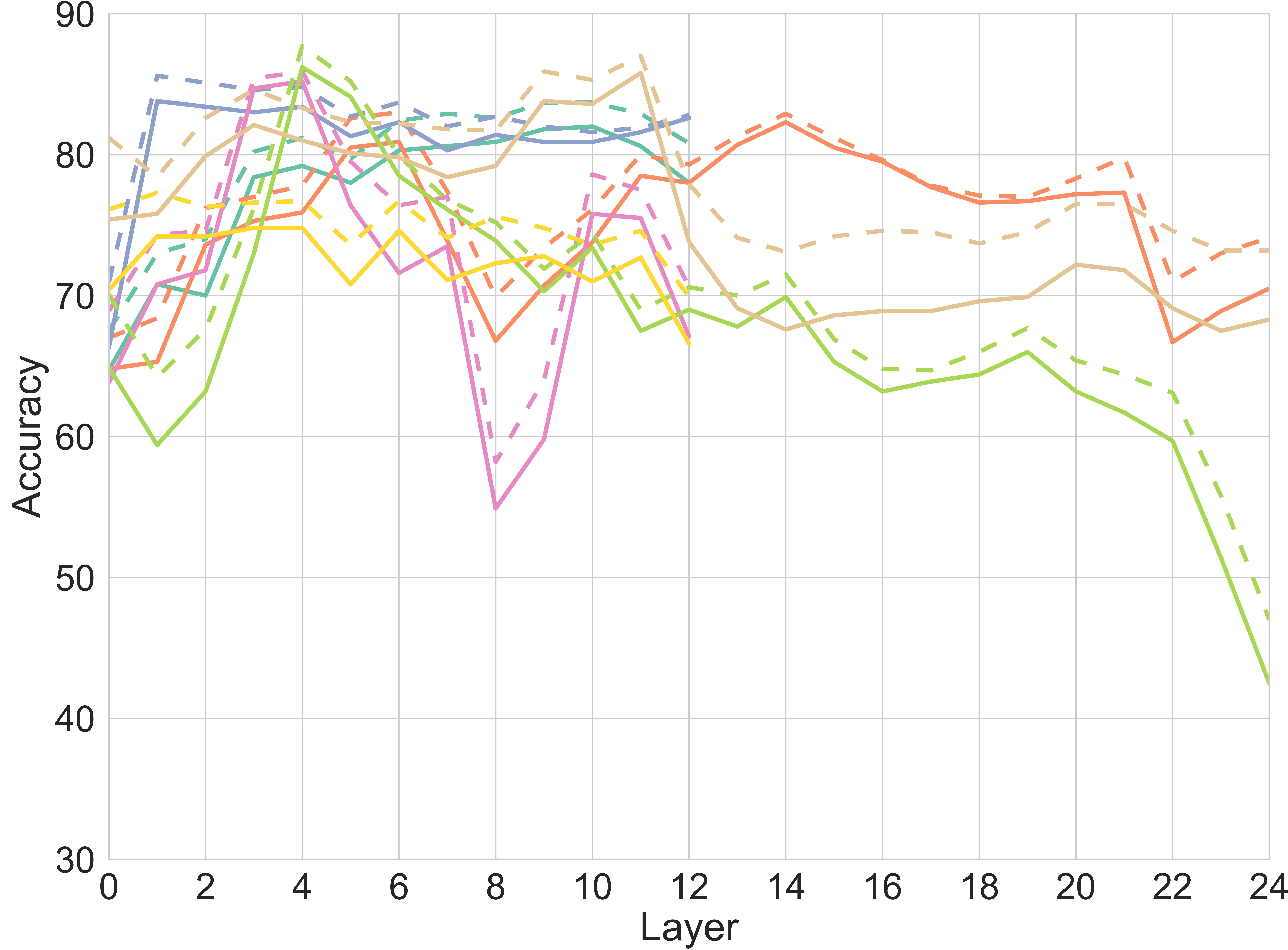
(a) Complexity (short)

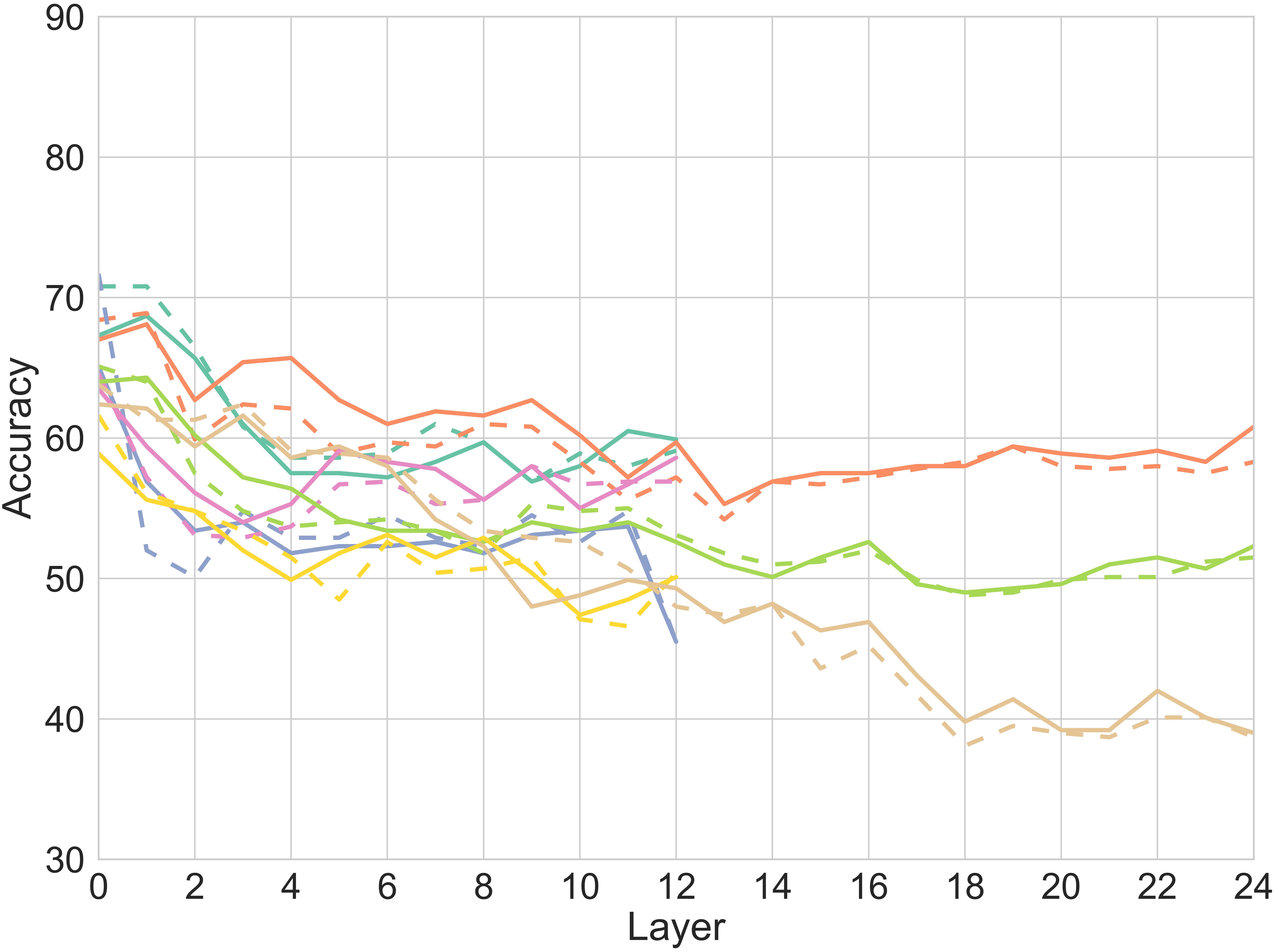
(b) Formality (short)

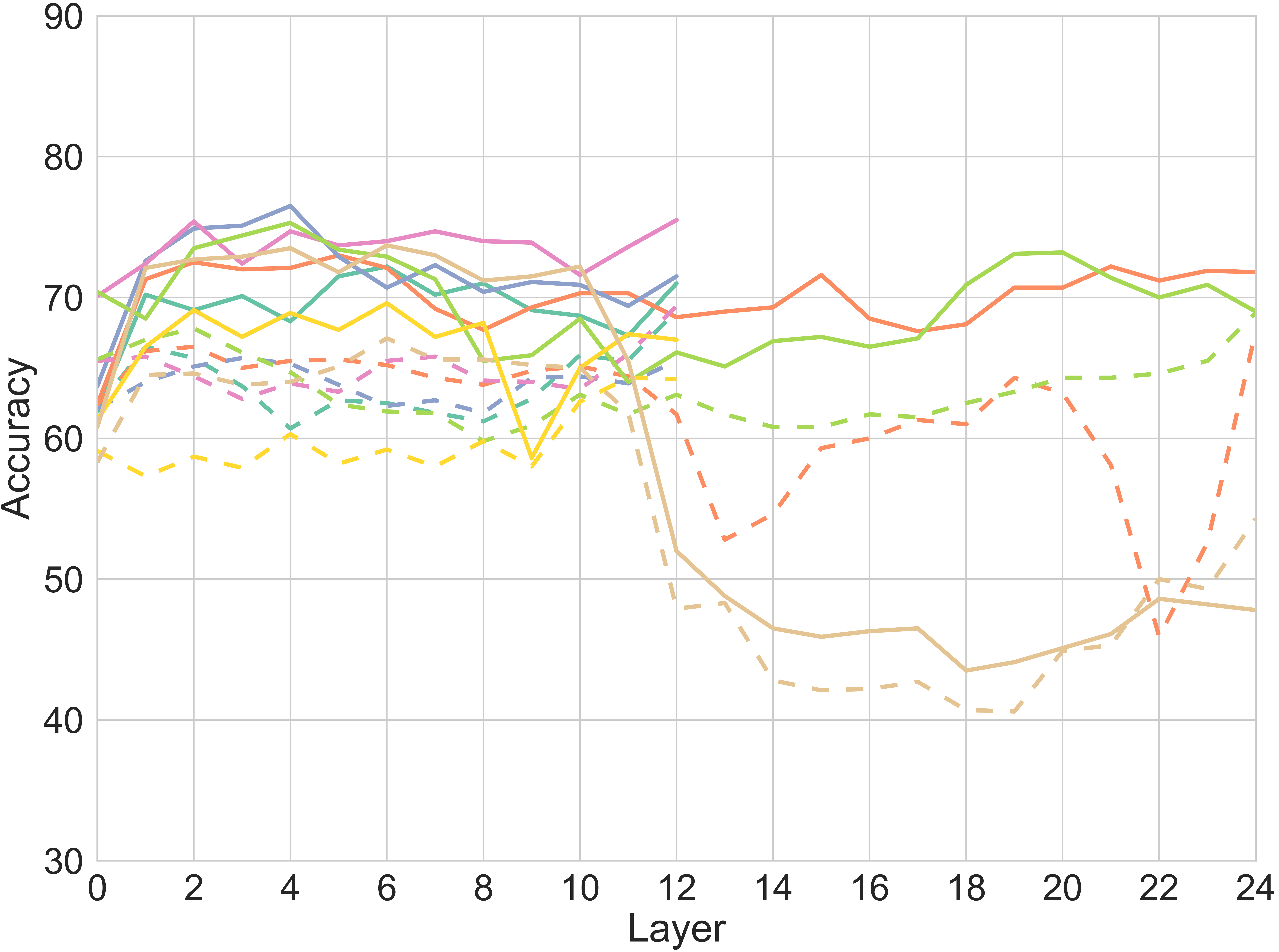
(c) Complexity (long)

(d) Formality (long)

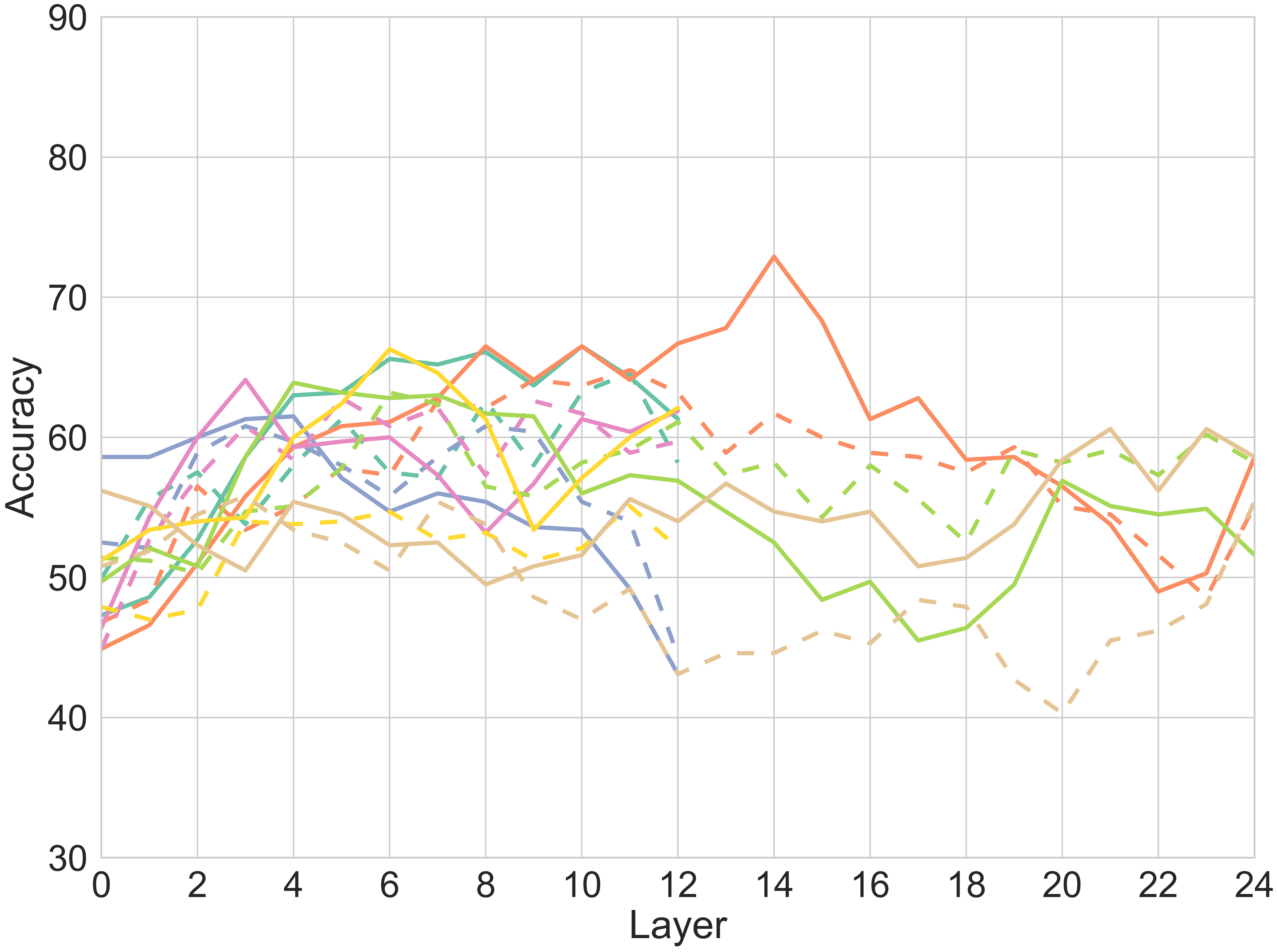
(e) Figurativeness (long)

Figure 6: Performance change across layers of different LMs (under the single-layer setting).

Regarding the performance change across layers, in addition to the plots shown in Section 5.1 under the layer aggregation setting, here we present the results under the single-layer setting in Figure 6. Compared to layer aggregation, the results here are noticeably more chaotic, exhibiting no clear general trends.

C.3 Performance by Text Length Under Single-layer Setting

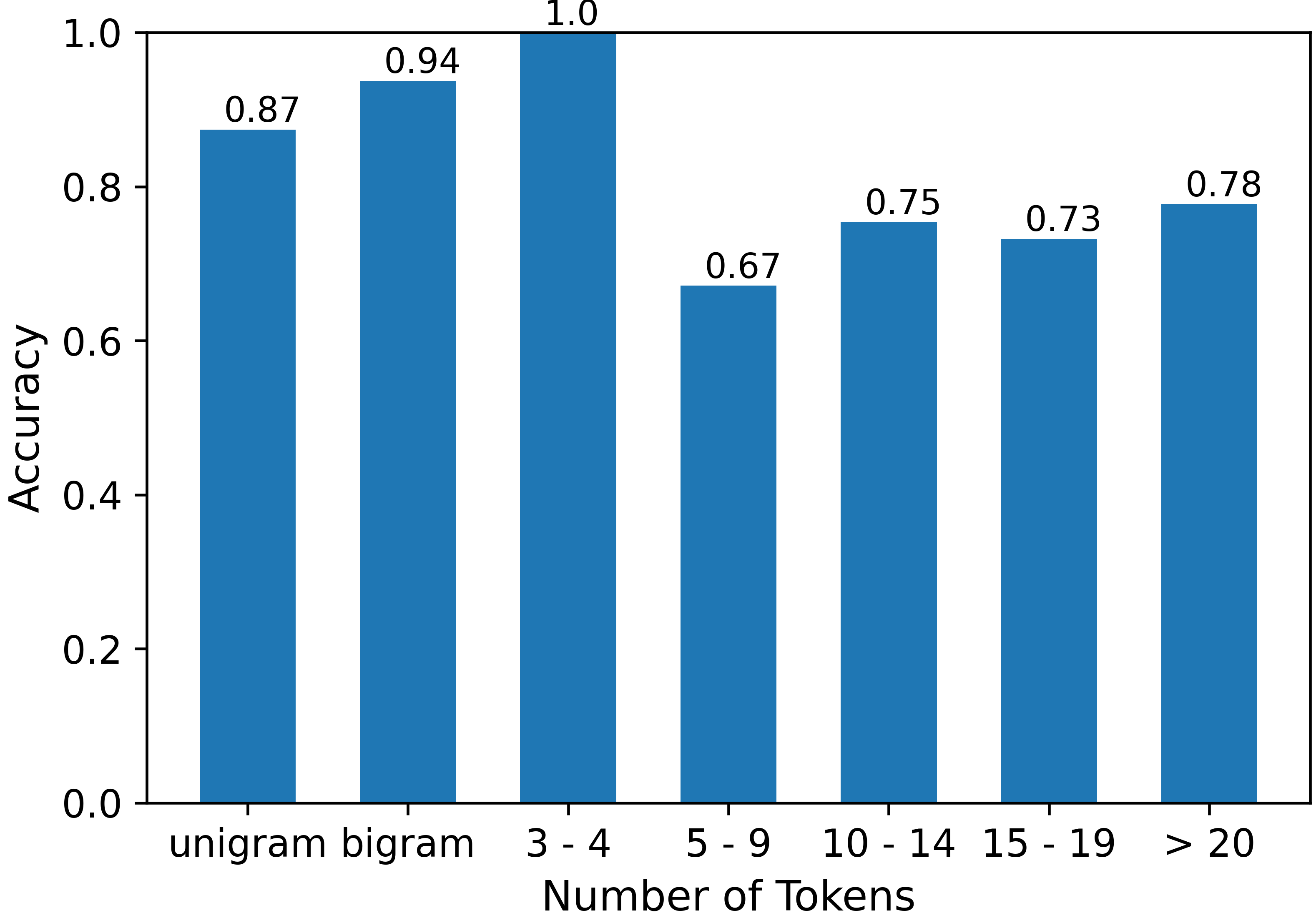
(a) Complexity

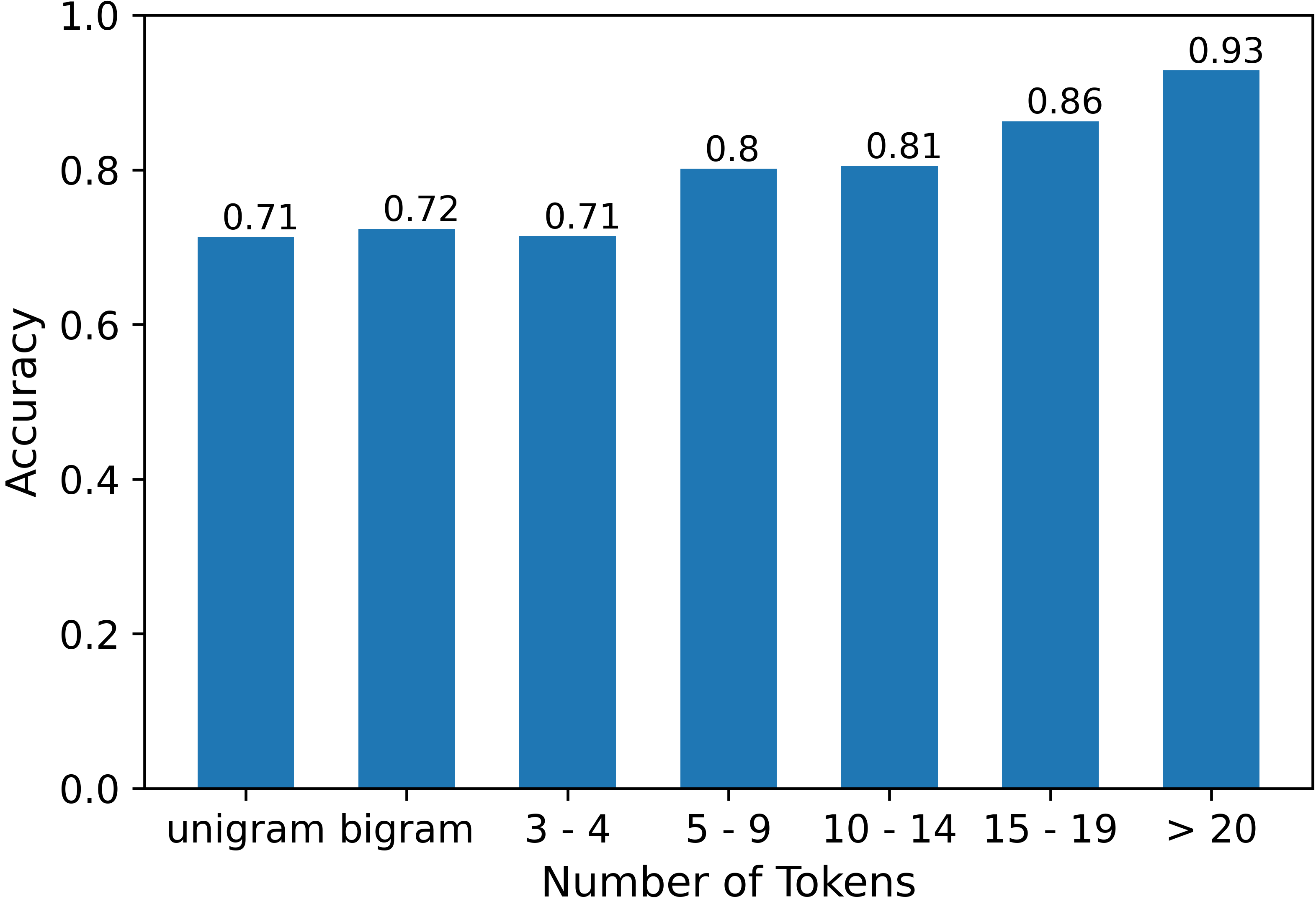
(b) Formality

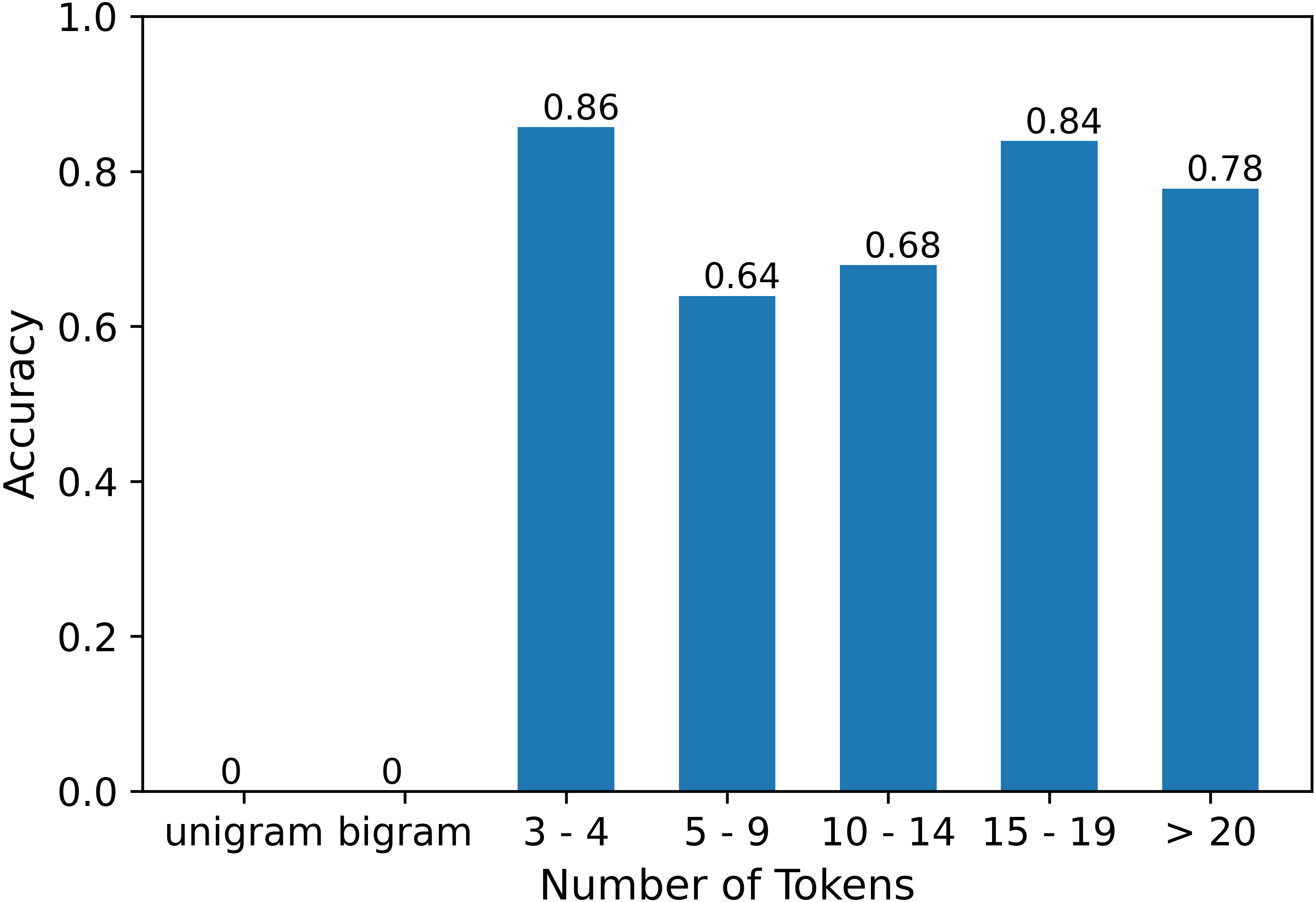
(c) Figurativeness

Figure 7: Optimal performance over different bins of text length (under the single-layer setting).

Similarly, we also present the performance change by text length under the single-layer setting in Figure 7, complementing the results under the layer aggregation setting in Section 5.2. The trends are mostly similar between the two settings.

C.4 Effect of Anisotropy Reduction

Pooling	Stats	Complexity		Formality		Figurativeness
		short	long	short	long	long
Mean	2 beats 1 (%)	25.2	21.3	44.9	40.2	74.0
	acc gain	-5.9	-5.0	-0.2	-8.2	4.3
Max	2 beats 1 (%)	18.9	28.3	48.0	44.1	59.1
	acc gain	-7.4	-2.2	0.0	-0.3	1.7
Average	2 beats 1 (%)	22.0	24.8	46.5	42.1	66.5
	acc gain	-6.7	-3.6	-0.1	-4.2	3.0

(a) All-but-the-top (single-layer)

Pooling	Stats	Complexity		Formality		Figurativeness
		short	long	short	long	long
Mean	2 beats 1 (%)	27.6	6.3	46.5	26.8	75.6
	acc gain	-4.6	-8.1	-0.2	-14.7	5.6
Max	2 beats 1 (%)	16.5	15.0	47.2	38.6	65.4
	acc gain	-6.8	-5.3	-0.1	-4.0	3.1
Average	2 beats 1 (%)	22.0	10.6	46.9	32.7	70.5
	acc gain	-5.7	-6.7	-0.1	-9.4	4.3

(b) All-but-the-top (layer aggregation)

Pooling	Stats	Complexity		Formality		Figurativeness
		short	long	short	long	long
Mean	2 beats 1 (%)	66.9	18.1	79.5	69.3	50.4
	acc gain	3.9	-3.6	5.5	9.3	-0.7
Max	2 beats 1 (%)	50.4	17.3	80.3	67.7	38.6
	acc gain	1.6	-4.8	5.1	12.1	-2.1
Average	2 beats 1 (%)	58.7	17.7	79.9	68.5	44.5
	acc gain	2.7	-4.2	5.3	10.7	-1.4

(c) Standardization (single-layer)

Pooling	Stats	Complexity		Formality		Figurativeness
		short	long	short	long	long
Mean	2 beats 1 (%)	86.6	15.0	93.7	60.6	72.4
	acc gain	6.8	-3.2	7.2	2.5	2.5
Max	2 beats 1 (%)	69.3	9.4	84.3	63.8	40.9
	acc gain	4.0	-6.1	5.7	7.6	-0.8
Average	2 beats 1 (%)	78.0	12.2	89.0	62.2	56.7
	acc gain	5.4	-4.7	6.5	5.0	0.8

(d) Standardization (layer aggregation)

Pooling	Stats	Complexity		Formality		Figurativeness
		short	long	short	long	long
Mean	2 beats 1 (%)	48.8	29.1	46.5	46.5	48.8
	acc gain	0.1	-1.1	-0.4	1.0	-0.3
Max	2 beats 1 (%)	47.2	38.6	46.5	63.8	52.0
	acc gain	-0.3	-0.8	-0.3	3.3	0.4
Average	2 beats 1 (%)	48.0	33.9	46.5	55.1	50.4
	acc gain	-0.1	-1.0	-0.4	2.1	0.1

(e) Rank-based (single-layer)

Pooling	Stats	Complexity		Formality		Figurativeness
		short	long	short	long	long
Mean	2 beats 1 (%)	54.3	32.3	33.1	36.2	54.3
	acc gain	-0.2	-1.8	-0.9	0.5	-0.2
Max	2 beats 1 (%)	54.3	48.0	43.3	71.7	62.2
	acc gain	-0.4	0.3	-0.5	3.2	0.8
Average	2 beats 1 (%)	54.3	40.2	38.2	53.9	58.3
	acc gain	-0.3	-0.8	-0.7	1.9	0.3

(f) Rank-based (layer aggregation)

Table 9: Effect of three different anisotropy reduction strategies: all-but-the-top, standardization, and rank-based (3 rows). Each strategy is evaluated under single-layer and layer aggregation settings (2 columns). In each table, “2 beats 1 (%)” refers to the percentage of cases where the performance with the anisotropy reduction strategy is at least as high as the performance without it, under the same configuration (LM & layer). “Acc gain” stands for the average accuracy gain of applying the anisotropy reduction strategy across all configurations. Positive accuracy gains are highlighted in green, negative ones in pink.

Table 9 shows the effect of using the 3 different anisotropy reduction strategies, across all LM and layer configurations. All-but-the-top only works for figurativeness; rank-based only works for formality (long); and standardization works slightly more generally, for complexity (short), formality (short), and formality (long). Nevertheless, overall there is no strategy that works universally under every condition.

References

- Adi et al. (2017) Yossi Adi, Einat Kermany, Yonatan Belinkov, Ofer Lavi, and Yoav Goldberg. 2017. Fine-grained Analysis of Sentence Embeddings Using Auxiliary Prediction Tasks. arXiv:1608.04207 [cs]. ArXiv: 1608.04207.
- Apidianaki (2023) Marianna Apidianaki. 2023. From Word Types to Tokens and Back: A Survey of Approaches to Word Meaning Representation and Interpretation. Computational Linguistics, pages 1–58.
- Birke and Sarkar (2006) Julia Birke and Anoop Sarkar. 2006. A clustering approach for nearly unsupervised recognition of nonliteral language. In 11th Conference of the European Chapter of the Association for Computational Linguistics, pages 329–336, Trento, Italy. Association for Computational Linguistics.
- Bojanowski et al. (2017) Piotr Bojanowski, Edouard Grave, Armand Joulin, and Tomas Mikolov. 2017. Enriching Word Vectors with Subword Information. Transactions of the Association for Computational Linguistics, 5:135–146.
- Bolukbasi et al. (2016) Tolga Bolukbasi, Kai-Wei Chang, James Y Zou, Venkatesh Saligrama, and Adam T Kalai. 2016. Man is to Computer Programmer as Woman is to Homemaker? Debiasing Word Embeddings. In Advances in Neural Information Processing Systems 29, pages 4349–4357. Barcelona, Spain.
- Brants (2006) Thorsten Brants. 2006. Web 1t 5-gram version 1. http://www. ldc. upenn. edu/Catalog/CatalogEntry. jsp? catalogId= LDC2006T13.
- Brooke et al. (2010) Julian Brooke, Tong Wang, and Graeme Hirst. 2010. Automatic acquisition of lexical formality. In Coling 2010: Posters, pages 90–98, Beijing, China. Coling 2010 Organizing Committee.
- Cai et al. (2021) Xingyu Cai, Jiaji Huang, Yuchen Bian, and Kenneth Church. 2021. Isotropy in the Contextual Embedding Space: Clusters and Manifolds. In Proceedings of the International Conference on Learning Representations (ICLR), Online.
- Chakrabarty et al. (2022) Tuhin Chakrabarty, Arkadiy Saakyan, Debanjan Ghosh, and Smaranda Muresan. 2022. FLUTE: Figurative language understanding through textual explanations. In Proceedings of the 2022 Conference on Empirical Methods in Natural Language Processing, pages 7139–7159, Abu Dhabi, United Arab Emirates. Association for Computational Linguistics.
- Chang et al. (2022) Tyler Chang, Zhuowen Tu, and Benjamin Bergen. 2022. The geometry of multilingual language model representations. In Proceedings of the 2022 Conference on Empirical Methods in Natural Language Processing, pages 119–136, Abu Dhabi, United Arab Emirates. Association for Computational Linguistics.
- Conneau et al. (2020) Alexis Conneau, Kartikay Khandelwal, Naman Goyal, Vishrav Chaudhary, Guillaume Wenzek, Francisco Guzmán, Edouard Grave, Myle Ott, Luke Zettlemoyer, and Veselin Stoyanov. 2020. Unsupervised cross-lingual representation learning at scale. In Proceedings of the 58th Annual Meeting of the Association for Computational Linguistics, pages 8440–8451, Online. Association for Computational Linguistics.
- Conneau et al. (2018) Alexis Conneau, German Kruszewski, Guillaume Lample, Loïc Barrault, and Marco Baroni. 2018. What you can cram into a single $&!#* vector: Probing sentence embeddings for linguistic properties. In Proceedings of the 56th Annual Meeting of the Association for Computational Linguistics (Volume 1: Long Papers), pages 2126–2136, Melbourne, Australia. Association for Computational Linguistics.
- Dev and Phillips (2019) Sunipa Dev and Jeff M Phillips. 2019. Attenuating Bias in Word Vectors. In Proceedings of the 22nd International Conference on Artificial Intelligence and Statistics (AISTATS), Naha, Okinawa, Japan.
- Devlin et al. (2019) Jacob Devlin, Ming-Wei Chang, Kenton Lee, and Kristina Toutanova. 2019. BERT: Pre-training of deep bidirectional transformers for language understanding. In Proceedings of the 2019 Conference of the North American Chapter of the Association for Computational Linguistics: Human Language Technologies, Volume 1 (Long and Short Papers), pages 4171–4186, Minneapolis, Minnesota. Association for Computational Linguistics.
- Ebrahimi et al. (2018) Javid Ebrahimi, Anyi Rao, Daniel Lowd, and Dejing Dou. 2018. HotFlip: White-Box Adversarial Examples for Text Classification. In Proceedings of the 56th Annual Meeting of the Association for Computational Linguistics (Volume 2: Short Papers), pages 31–36, Melbourne, Australia. Association for Computational Linguistics.
- Edmonds and Hirst (2002) Philip Edmonds and Graeme Hirst. 2002. Near-Synonymy and Lexical Choice. Computational Linguistics, 28(2):105–144.
- Ethayarajh (2019) Kawin Ethayarajh. 2019. How Contextual are Contextualized Word Representations? Comparing the Geometry of BERT, ELMo, and GPT-2 Embeddings. In Proceedings of the 2019 Conference on Empirical Methods in Natural Language Processing and the 9th International Joint Conference on Natural Language Processing (EMNLP-IJCNLP), pages 55–65, Hong Kong, China. Association for Computational Linguistics.
- Ettinger (2020) Allyson Ettinger. 2020. What BERT Is Not: Lessons from a New Suite of Psycholinguistic Diagnostics for Language Models. Transactions of the Association for Computational Linguistics, 8:34–48.
- Ettinger et al. (2016) Allyson Ettinger, Ahmed Elgohary, and Philip Resnik. 2016. Probing for semantic evidence of composition by means of simple classification tasks. In Proceedings of the 1st Workshop on Evaluating Vector-Space Representations for NLP, pages 134–139, Berlin, Germany. Association for Computational Linguistics.
- Ganitkevitch et al. (2013) Juri Ganitkevitch, Benjamin Van Durme, and Chris Callison-Burch. 2013. PPDB: The paraphrase database. In Proceedings of the 2013 Conference of the North American Chapter of the Association for Computational Linguistics: Human Language Technologies, pages 758–764, Atlanta, Georgia. Association for Computational Linguistics.
- Gao et al. (2019) Jun Gao, Di He, Xu Tan, Tao Qin, Liwei Wang, and Tieyan Liu. 2019. Representation Degeneration Problem in Training Natural Language Generation Models. In International Conference on Learning Representations (ICLR), New Orleans, LA, USA.
- Garí Soler and Apidianaki (2020) Aina Garí Soler and Marianna Apidianaki. 2020. BERT Knows Punta Cana is not just beautiful, it’s gorgeous: Ranking Scalar Adjectives with Contextualised Representations. In Proceedings of the 2020 Conference on Empirical Methods in Natural Language Processing (EMNLP), pages 7371–7385, Online. Association for Computational Linguistics.
- Garí Soler and Apidianaki (2021a) Aina Garí Soler and Marianna Apidianaki. 2021a. Let’s Play Mono-Poly: BERT Can Reveal Words’ Polysemy Level and Partitionability into Senses. Transactions of the Association for Computational Linguistics, 9:825–844.
- Garí Soler and Apidianaki (2021b) Aina Garí Soler and Marianna Apidianaki. 2021b. Scalar Adjective Identification and Multilingual Ranking. In Proceedings of the 2021 Conference of the North American Chapter of the Association for Computational Linguistics: Human Language Technologies, pages 4653–4660, Online. Association for Computational Linguistics.
- Gutiérrez et al. (2016) E. Dario Gutiérrez, Ekaterina Shutova, Tyler Marghetis, and Benjamin Bergen. 2016. Literal and metaphorical senses in compositional distributional semantic models. In Proceedings of the 54th Annual Meeting of the Association for Computational Linguistics (Volume 1: Long Papers), pages 183–193, Berlin, Germany. Association for Computational Linguistics.
- Hewitt and Liang (2019) John Hewitt and Percy Liang. 2019. Designing and interpreting probes with control tasks. In Proceedings of the 2019 Conference on Empirical Methods in Natural Language Processing and the 9th International Joint Conference on Natural Language Processing (EMNLP-IJCNLP), pages 2733–2743, Hong Kong, China. Association for Computational Linguistics.
- Hewitt and Manning (2019) John Hewitt and Christopher D. Manning. 2019. A Structural Probe for Finding Syntax in Word Representations. In Proceedings of the 2019 Conference of the North American Chapter of the Association for Computational Linguistics: Human Language Technologies, Volume 1 (Long and Short Papers), pages 4129–4138, Minneapolis, Minnesota. Association for Computational Linguistics.
- Jeretic et al. (2020) Paloma Jeretic, Alex Warstadt, Suvrat Bhooshan, and Adina Williams. 2020. Are Natural Language Inference Models IMPPRESsive? Learning IMPlicature and PRESupposition. In Proceedings of the 58th Annual Meeting of the Association for Computational Linguistics.
- Kauchak (2013) David Kauchak. 2013. Improving text simplification language modeling using unsimplified text data. In Proceedings of the 51st Annual Meeting of the Association for Computational Linguistics (Volume 1: Long Papers), pages 1537–1546, Sofia, Bulgaria. Association for Computational Linguistics.
- Kozlowski et al. (2019) Austin C. Kozlowski, Matt Taddy, and James A. Evans. 2019. The geometry of culture: Analyzing the meanings of class through word embeddings. American Sociological Review, 84(5):905–949.
- Kriz et al. (2018) Reno Kriz, Eleni Miltsakaki, Marianna Apidianaki, and Chris Callison-Burch. 2018. Simplification Using Paraphrases and Context-Based Lexical Substitution. In Proceedings of the 2018 Conference of the North American Chapter of the Association for Computational Linguistics: Human Language Technologies, Volume 1 (Long Papers), pages 207–217, New Orleans, Louisiana. Association for Computational Linguistics.
- Linzen et al. (2016) Tal Linzen, Emmanuel Dupoux, and Yoav Goldberg. 2016. Assessing the Ability of LSTMs to Learn Syntax-Sensitive Dependencies. Transactions of the Association for Computational Linguistics, 4:521–535.
- Liu et al. (2019) Yinhan Liu, Myle Ott, Naman Goyal, Jingfei Du, Mandar Joshi, Danqi Chen, Omer Levy, Mike Lewis, Luke Zettlemoyer, and Veselin Stoyanov. 2019. RoBERTa: A Robustly Optimized BERT Pretraining Approach. arXiv:1907.11692.
- Lovering et al. (2020) Charles Lovering, Rohan Jha, Tal Linzen, and Ellie Pavlick. 2020. Information-theoretic Probing Explains Reliance on Spurious Features.
- Mu and Viswanath (2018) Jiaqi Mu and Pramod Viswanath. 2018. All-but-the-Top: Simple and Effective Postprocessing for Word Representations. In International Conference on Learning Representations (ICLR), Vancouver, Canada.
- Pavlick and Callison-Burch (2016) Ellie Pavlick and Chris Callison-Burch. 2016. Simple PPDB: A Paraphrase Database for Simplification. In Proceedings of the 54th Annual Meeting of the Association for Computational Linguistics (Volume 2: Short Papers), pages 143–148, Berlin, Germany. Association for Computational Linguistics.
- Pavlick and Nenkova (2015) Ellie Pavlick and Ani Nenkova. 2015. Inducing lexical style properties for paraphrase and genre differentiation. In Proceedings of the 2015 Conference of the North American Chapter of the Association for Computational Linguistics: Human Language Technologies, pages 218–224, Denver, Colorado. Association for Computational Linguistics.
- Pennington et al. (2014) Jeffrey Pennington, Richard Socher, and Christopher Manning. 2014. GloVe: Global vectors for word representation. In Proceedings of the 2014 Conference on Empirical Methods in Natural Language Processing (EMNLP), pages 1532–1543, Doha, Qatar. Association for Computational Linguistics.
- Petroni et al. (2019) Fabio Petroni, Tim Rocktäschel, Sebastian Riedel, Patrick Lewis, Anton Bakhtin, Yuxiang Wu, and Alexander Miller. 2019. Language Models as Knowledge Bases? In Proceedings of the 2019 Conference on Empirical Methods in Natural Language Processing and the 9th International Joint Conference on Natural Language Processing (EMNLP-IJCNLP), pages 2463–2473, Hong Kong, China. Association for Computational Linguistics.
- Piccirilli and Schulte Im Walde (2022) Prisca Piccirilli and Sabine Schulte Im Walde. 2022. What drives the use of metaphorical language? negative insights from abstractness, affect, discourse coherence and contextualized word representations. In Proceedings of the 11th Joint Conference on Lexical and Computational Semantics, pages 299–310, Seattle, Washington. Association for Computational Linguistics.
- Pimentel et al. (2020) Tiago Pimentel, Rowan Hall Maudslay, Damian Blasi, and Ryan Cotterell. 2020. Speakers Fill Lexical Semantic Gaps with Context. In Proceedings of the 2020 Conference on Empirical Methods in Natural Language Processing (EMNLP), pages 4004–4015, Online. Association for Computational Linguistics.
- Raganato and Tiedemann (2018) Alessandro Raganato and Jörg Tiedemann. 2018. An analysis of encoder representations in transformer-based machine translation. In Proceedings of the 2018 EMNLP Workshop BlackboxNLP: Analyzing and Interpreting Neural Networks for NLP, pages 287–297, Brussels, Belgium. Association for Computational Linguistics.
- Rajaee and Pilehvar (2021) Sara Rajaee and Mohammad Taher Pilehvar. 2021. A Cluster-based Approach for Improving Isotropy in Contextual Embedding Space. In Proceedings of the 59th Annual Meeting of the Association for Computational Linguistics and the 11th International Joint Conference on Natural Language Processing (Volume 2: Short Papers), pages 575–584, Online. Association for Computational Linguistics.
- Rao and Tetreault (2018) Sudha Rao and Joel Tetreault. 2018. Dear sir or madam, may I introduce the GYAFC dataset: Corpus, benchmarks and metrics for formality style transfer. In Proceedings of the 2018 Conference of the North American Chapter of the Association for Computational Linguistics: Human Language Technologies, Volume 1 (Long Papers), pages 129–140, New Orleans, Louisiana. Association for Computational Linguistics.
- Ravichander et al. (2020) Abhilasha Ravichander, Eduard Hovy, Kaheer Suleman, Adam Trischler, and Jackie Chi Kit Cheung. 2020. On the systematicity of probing contextualized word representations: The case of hypernymy in BERT. In Proceedings of the Ninth Joint Conference on Lexical and Computational Semantics, pages 88–102, Barcelona, Spain (Online). Association for Computational Linguistics.
- Schuster et al. (2020) Sebastian Schuster, Yuxing Chen, and Judith Degen. 2020. Harnessing the linguistic signal to predict scalar inferences. In Proceedings of the 58th Annual Meeting of the Association for Computational Linguistics.
- Shardlow (2013) Matthew Shardlow. 2013. A Comparison of Techniques to Automatically Identify Complex Words. In 51st Annual Meeting of the Association for Computational Linguistics Proceedings of the Student Research Workshop, pages 103–109, Sofia, Bulgaria. Association for Computational Linguistics.
- Stowe et al. (2022) Kevin Stowe, Prasetya Utama, and Iryna Gurevych. 2022. IMPLI: Investigating NLI models’ performance on figurative language. In Proceedings of the 60th Annual Meeting of the Association for Computational Linguistics (Volume 1: Long Papers), pages 5375–5388, Dublin, Ireland. Association for Computational Linguistics.
- Thukral et al. (2021) Shivin Thukral, Kunal Kukreja, and Christian Kavouras. 2021. Probing Language Models for Understanding of Temporal Expressions. In Proceedings of the Fourth BlackboxNLP Workshop on Analyzing and Interpreting Neural Networks for NLP, pages 396–406, Punta Cana, Dominican Republic. Association for Computational Linguistics.
- Timkey and van Schijndel (2021) William Timkey and Marten van Schijndel. 2021. All Bark and No Bite: Rogue Dimensions in Transformer Language Models Obscure Representational Quality. In Proceedings of the 2021 Conference on Empirical Methods in Natural Language Processing, pages 4527–4546, Online and Punta Cana, Dominican Republic. Association for Computational Linguistics.
- Tsvetkov et al. (2013) Yulia Tsvetkov, Elena Mukomel, and Anatole Gershman. 2013. Cross-lingual metaphor detection using common semantic features. In Proceedings of the First Workshop on Metaphor in NLP, pages 45–51, Atlanta, Georgia. Association for Computational Linguistics.
- Veldhoen et al. (2016) Sara Veldhoen, Dieuwke Hupkes, Willem H Zuidema, et al. 2016. Diagnostic classifiers revealing how neural networks process hierarchical structure. In CoCo@ NIPS, pages 69–77. Barcelona.
- Voita and Titov (2020) Elena Voita and Ivan Titov. 2020. Information-Theoretic Probing with Minimum Description Length. arXiv:2003.12298 [cs]. ArXiv: 2003.12298.
- Vulić et al. (2020) Ivan Vulić, Edoardo Maria Ponti, Robert Litschko, Goran Glavaš, and Anna Korhonen. 2020. Probing pretrained language models for lexical semantics. In Proceedings of the 2020 Conference on Empirical Methods in Natural Language Processing (EMNLP), pages 7222–7240, Online. Association for Computational Linguistics.
- Wallace et al. (2019) Eric Wallace, Shi Feng, Nikhil Kandpal, Matt Gardner, and Sameer Singh. 2019. Universal Adversarial Triggers for Attacking and Analyzing NLP. In Proceedings of the 2019 Conference on Empirical Methods in Natural Language Processing and the 9th International Joint Conference on Natural Language Processing (EMNLP-IJCNLP), pages 2153–2162, Hong Kong, China. Association for Computational Linguistics.
- Wartena (2022) Christian Wartena. 2022. On the geometry of concreteness. In Proceedings of the 7th Workshop on Representation Learning for NLP, pages 204–212, Dublin, Ireland. Association for Computational Linguistics.
- Yanaka et al. (2020) Hitomi Yanaka, Koji Mineshima, Daisuke Bekki, and Kentaro Inui. 2020. Do Neural Models Learn Systematicity of Monotonicity Inference in Natural Language? In Proceedings of the 58th Annual Meeting of the Association for Computational Linguistics.
- Zhelezniak et al. (2019) Vitalii Zhelezniak, Aleksandar Savkov, April Shen, and Nils Hammerla. 2019. Correlation coefficients and semantic textual similarity. In Proceedings of the 2019 Conference of the North American Chapter of the Association for Computational Linguistics: Human Language Technologies, Volume 1 (Long and Short Papers), pages 951–962, Minneapolis, Minnesota. Association for Computational Linguistics.