HySST: A Stable Sparse Rapidly-Exploring Random Trees Optimal Motion Planning Algorithm for Hybrid Dynamical Systems*

Abstract

This paper proposes a stable sparse rapidly-exploring random trees (SST) algorithm to solve the optimal motion planning problem for hybrid systems. At each iteration, the proposed algorithm, called HySST, selects a vertex with the lowest cost among all the vertices within the neighborhood of a randomly selected sample and then extends the search tree by flow or jump, which is also chosen randomly when both regimes are possible. In addition, HySST maintains a static set of witness points such that all the vertices within the neighborhood of each witness are pruned except the vertex with the lowest cost. Through a definition of concatenation of functions defined on hybrid time domains, we show that HySST is asymptotically near optimal, namely, the probability of failing to find a motion plan such that its cost is close to the optimal cost approaches zero as the number of iterations of the algorithm increases to infinity. This property is guaranteed under mild conditions on the data defining the motion plan, which include a relaxation of the usual positive clearance assumption imposed in the literature of classical systems. The proposed algorithm is applied to an actuated bouncing ball system and a collision-resilient tensegrity multicopter system so as to highlight its generality and computational features.

I Introduction

Motion planning consists of finding a state trajectory and associated inputs that connect the initial and final state sets while satisfying the dynamics of the systems and given safety requirements. Motion planning for purely continuous-time systems and purely discrete-time systems has been well studied in the literature; see e.g., [1]. In recent years, several (feasible) motion planning algorithms have been developed, including graph search algorithms [2], artificial potential field methods [3] and sampling-based algorithms. The sampling-based algorithms have drawn much attention in recent years because of their fast exploration speed for high dimensional problems and theoretical guarantees; specially, probabilistic completeness, which means that the probability of failing to find a motion plan converges to zero, as the number of samples approaches infinity. Two popular sampling-based algorithms are the probabilistic roadmap (PRM) algorithm [4] and the rapidly-exploring random tree (RRT) algorithm [5]. The PRM method relies on the existence of a steering function returning the solution of a two-point boundary value problem (TPBVP). Unfortunately, solutions to TPBVPs are difficult to generate for most dynamical systems. On the other hand, RRT algorithm does not require a steering function. Arguably, RRT is perhaps the most successful algorithm to solve feasible motion planning problems.

A feasible solution is not sufficient in most applications as the quality of the solution returned by the motion planning algorithms is key [6]. It has been shown in [7] that the solution returned by RRT converges to a sub-optimal solution. Therefore, variants of PRM and RRT, such as PRM* and RRT* [8], have been developed to solve optimal motion planning problems with guaranteed asymptotic optimality. However, both PRM* and RRT* require a steering function, which prevents them from being widely applied. On the other hand, the stable sparse RRT (SST) algorithm [9] does not require a steering function and is guaranteed to be asymptotically near optimal, which means that the probability of finding a solution that has a cost close to the minimal cost converges to one as the number of iterations goes to infinity.

The aforementioned motion planning algorithms have been widely applied to purely continuous-time and purely discrete-time systems. However, much less efforts have been devoted to the motion planning for hybrid systems. In our previous work [10], a feasible motion planning problem is formulated for hybrid system given in terms of hybrid equations as in [11], which is a general framework that captures a broad class of hybrid systems. In [10], the hybrid RRT algorithm is designed to solve the feasible motion planning problem for such systems with guaranteed probabilistic completeness. In this paper, we propose a motion planning algorithm for hybrid systems with the goal of assuring (asymptotic) optimality of the solution. We formulate the optimal motion planning problem for hybrid systems inspired by the feasible motion planning problems in [10]. Then, we design an SST-type algorithm to solve the optimal motion planning problem for hybrid systems. Following [9], the proposed algorithm, called HySST, incrementally constructs a search tree rooted in the initial state set toward the random samples. At first, HySST draws samples from the state space. Then, it selects a vertex such that the state associated with this vertex is within a ball centered at the random sample and has minimal cost. Next, HySST propagates the state trajectory from the state associated with the selected vertex, and adds a new vertex and edge from the propagated trajectory. In addition, HySST maintains a static set of state points, called witnesses, to represent the explored regions in the state space. HySST also employs a pruning process to guarantee that only a single vertex with lowest cost is kept within the neighborhood of each witness. We show that, under mild assumptions, HySST is asymptotically near-optimal. To the authors’ best knowledge, it is the first optimal RRT-type algorithm for systems with hybrid dynamics. The proposed algorithm is illustrated in an actuated bouncing ball system and a collision-resilient tensegrity multicopter system.

The remainder of the paper is structured as follows. Section II presents notation and preliminaries. Section III presents the problem statement and introduction of applications. Section IV presents the HySST algorithm. Section V presents the analysis of the asymptotic near optimality of HySST algorithm. Section VI presents the illustration of HySST in the examples. Proofs and more details are given [12].

II Notation and Preliminaries

II-A Notation

The real numbers are denoted as $\mathbb{R}$ and its nonnegative subset is denoted as $\mathbb{R}_{\geq 0}$. The set of nonnegative integers is denoted as $\mathbb{N}$. The notation $\operatorname{int}S$ denotes the interior of the set $S$. The notation $\overline{S}$ denotes the closure of the set $S$. The notation $\partial S$ denotes the boundary of the set $S$. The notation $\mathop{\rm rge}f$ denotes the range of the function $f$. The notation $\mathbb{B}$ denotes the closed unit ball of appropriate dimension in the Euclidean norm. The notation $c+r\mathbb{B}$ denotes the closed ball of appropriate dimension in the Euclidean norm centered at $c$ with radius $r$. Given sets $P\subset\mathbb{R}^{n}$ and $Q\subset\mathbb{R}^{n}$, the Minkowski sum of $P$ and $Q$, denoted as $P+Q$, is the set $\{p+q:p\in P,q\in Q\}$.

II-B Preliminaries

A hybrid system $\mathcal{H}$ with inputs is modeled as [13]

$$\mathcal{H}:\left\{\begin{aligned} \dot{x}&=f(x,u)&(x,u)\in C\\ x^{+}&=g(x,u)&(x,u)\in D\\ \end{aligned}\right.$$ (1)

where $x\in\mathbb{R}^{n}$ is the state, $u\in\mathbb{R}^{m}$ is the input, $C\subset\mathbb{R}^{n}\times\mathbb{R}^{m}$ represents the flow set, $f:\mathbb{R}^{n}\times\mathbb{R}^{m}\to\mathbb{R}^{n}$ represents the flow map, $D\subset\mathbb{R}^{n}\times\mathbb{R}^{m}$ represents the jump set, and $g:\mathbb{R}^{n}\times\mathbb{R}^{m}\to\mathbb{R}^{n}$ represents the jump map, respectively. The continuous evolution of $x$ is captured by the flow map $f$. The discrete evolution of $x$ is captured by the jump map $g$. The flow set $C$ collects the points where the state can evolve continuously. The jump set $D$ collects the points where jumps can occur.

Given a flow set $C$, the set $U_{C}:=\{u\in\mathbb{R}^{m}:\exists x\in\mathbb{R}^{n}\text{ such that }(x,u)\in C\}$ includes all possible input values that can be applied during flows. Similarly, given a jump set $D$, the set $U_{D}:=\{u\in\mathbb{R}^{m}:\exists x\in\mathbb{R}^{n}\text{ such that }(x,u)\in D\}$ includes all possible input values that can be applied at jumps. These sets satisfy $C\subset\mathbb{R}^{n}\times U_{C}$ and $D\subset\mathbb{R}^{n}\times U_{D}$. Given a set $K\subset\mathbb{R}^{n}\times U_{\star}$, where $\star$ is either $C$ or $D$, we define $\Pi_{\star}(K):=\{x:\exists u\in U_{\star}\text{ s.t. }(x,u)\in K\}$ as the projection of $K$ onto $\mathbb{R}^{n}$, and define $C^{\prime}:=\Pi_{C}(C)$ and $D^{\prime}:=\Pi_{D}(D)$.

In addition to ordinary time $t\in\mathbb{R}_{\geq 0}$, we employ $j\in\mathbb{N}$ to denote the number of jumps of the evolution of $x$ and $u$ for $\mathcal{H}$ in (1), leading to hybrid time $(t,j)$ for the parameterization of its solutions and inputs. The domain of a solution to $\mathcal{H}$ is given by a hybrid time domain. A hybrid time domain is defined as a subset $E$ of $\mathbb{R}_{\geq 0}\times\mathbb{N}$ that, for each $(T,J)\in E$, $E\cap([0,T]\times\{0,1,...,J\})$ can be written as $\cup_{j=0}^{J}([t_{j},t_{j+1}],j)$ for some finite sequence of times $0=t_{0}\leq t_{1}\leq t_{2}\leq...\leq t_{J+1}=T$. A hybrid arc $\phi:\mathop{\rm dom}\nolimits\phi\to\mathbb{R}^{n}$ is a function on a hybrid time domain that, for each $j\in\mathbb{N}$, $t\mapsto\phi(t,j)$ is locally absolutely continuous on each interval $I^{j}:=\{t:(t,j)\in\mathop{\rm dom}\nolimits\phi\}$ with nonempty interior. The definition of solution pair to a hybrid system is given as follows. For more details, see [11].

Definition II.1 (Solution pair to a hybrid system)

Given a pair of functions $\phi:\mathop{\rm dom}\nolimits\phi\to\mathbb{R}^{n}$ and $u:\mathop{\rm dom}\nolimits u\to\mathbb{R}^{m}$, $(\phi,u)$ is a solution pair to (1) if $\mathop{\rm dom}\nolimits(\phi,u):=\mathop{\rm dom}\nolimits\phi=\mathop{\rm dom}\nolimits u$ is a hybrid time domain, $(\phi(0,0),u(0,0))\in\overline{C}\cup D$, and the following hold:

1. For all $j\in\mathbb{N}$ such that $I^{j}$ has nonempty interior,

   1. the function $t\mapsto\phi(t,j)$ is locally absolutely continuous,

   2. $(\phi(t,j),u(t,j))\in C$ for all $t\in\operatorname{int}I^{j}$,

   3. the function $t\mapsto u(t,j)$ is Lebesgue measurable and locally bounded,

   4. for almost all $t\in I^{j}$, $\dot{\phi}(t,j)=f(\phi(t,j),u(t,j))$.

2. For all $(t,j)\in\mathop{\rm dom}\nolimits(\phi,u)$ such that $(t,j+1)\in\mathop{\rm dom}\nolimits(\phi,u)$,

   $$(\phi(t,j),u(t,j))\in D\quad\phi(t,j+1)=g(\phi(t,j),u(t,j)).$$

HySST requires concatenating solution pairs. The concatenation operation of solution pairs is defined next.

Definition II.2

(Concatenation operation) Given two functions $\phi_{1}:\mathop{\rm dom}\nolimits\phi_{1}\to\mathbb{R}^{n}$ and $\phi_{2}:\mathop{\rm dom}\nolimits\phi_{2}\to\mathbb{R}^{n}$, where $\mathop{\rm dom}\nolimits\phi_{1}$ and $\mathop{\rm dom}\nolimits\phi_{2}$ are hybrid time domains, $\phi_{2}$ can be concatenated to $\phi_{1}$ if $\phi_{1}$ is compact and $\phi:\mathop{\rm dom}\nolimits\phi\to\mathbb{R}^{n}$ is the concatenation of $\phi_{2}$ to $\phi_{1}$, denoted $\phi=\phi_{1}|\phi_{2}$, namely,

1. $\mathop{\rm dom}\nolimits\phi=\mathop{\rm dom}\nolimits\phi_{1}\cup(\mathop{\rm dom}\nolimits\phi_{2}+\{(T,J)\})$, where $(T,J)=\max\mathop{\rm dom}\nolimits\phi_{1}$ and the plus sign denotes Minkowski addition;

2. $\phi(t,j)=\phi_{1}(t,j)$ for all $(t,j)\in\mathop{\rm dom}\nolimits\phi_{1}\backslash\{(T,J)\}$ and $\phi(t,j)=\phi_{2}(t-T,j-J)$ for all $(t,j)\in\mathop{\rm dom}\nolimits\phi_{2}+\{(T,J)\}$.

III Problem Statement

The feasible motion planning problem for hybrid systems is defined in [10] as follows.

Problem 1

(Feasible motion planning) Given a hybrid system $\mathcal{H}$ with input $u\in\mathbb{R}^{m}$ and state $x\in\mathbb{R}^{n}$, the initial state set $X_{0}\subset\mathbb{R}^{n}$, the final state set $X_{f}\subset\mathbb{R}^{n}$, and the unsafe set $X_{u}\subset\mathbb{R}^{n}\times\mathbb{R}^{m}$, find a pair $(\phi,u):\mathop{\rm dom}\nolimits(\phi,u)\to\mathbb{R}^{n}\times\mathbb{R}^{m}$, namely, a motion plan, such that for some $(T,J)\in\mathop{\rm dom}\nolimits(\phi,u)$, the following hold:

1. $\phi(0,0)\in X_{0}$, namely, the initial state of the solution belongs to the given initial state set $X_{0}$;

2. $(\phi,u)$ is a solution pair to $\mathcal{H}$ as defined in Definition II.1;

3. $(T,J)$ is such that $\phi(T,J)\in X_{f}$, namely, the solution belongs to the final state set at hybrid time $(T,J)$;

4. $(\phi(t,j),u(t,j))\notin X_{u}$ for each $(t,j)\in\mathop{\rm dom}\nolimits(\phi,u)$ such that $t+j\leq T+J$, namely, the solution pair does not intersect with the unsafe set before its state trajectory reaches the final state set.

Therefore, given sets $X_{0}$, $X_{f}$ and $X_{u}$, and a hybrid system $\mathcal{H}$ with data $(C,f,D,g)$, a (feasible) motion planning problem $\mathcal{P}$ is formulated as $\mathcal{P}=(X_{0},X_{f},X_{u},(C,f,D,g)).$

Let $\Sigma$ denote the set of all solution pairs to $\mathcal{H}$. Let $\Sigma_{\phi}$ denote the set of state trajectories of all the solution pairs in $\Sigma$. The optimal motion planning problem for hybrid systems consists of finding a feasible motion plan with minimum cost [8, Problem 3].

Problem 2

(Optimal motion planning) Given a motion planning problem $\mathcal{P}=(X_{0},X_{f},X_{u},(C,f,D,g))$ and a cost functional $c:\Sigma_{\phi}\to\mathbb{R}_{\geq 0}$ where $\Sigma:=\{(\phi,u):(\phi,u)\text{ is a solution pair to }(C,f,D,g)\}$ and $\Sigma_{\phi}:=\{\phi:\exists u:\mathop{\rm dom}\nolimits\phi\to\mathbb{R}^{m}\text{ such that }(\phi,u)\in\Sigma\}$, find a feasible motion plan $(\phi^{*},u^{*})$ to Problem 1 such that $(\phi^{*},u^{*})=\operatorname*{arg\,min}_{(\phi,u)\in\Sigma}c(\phi)$. Given sets $X_{0}$, $X_{f}$ and $X_{u}$, a hybrid system $\mathcal{H}$ with data $(C,f,D,g)$, and a cost functional $c$, an optimal motion planning problem $\mathcal{P}^{*}$ is formulated as $\mathcal{P}^{*}=(X_{0},X_{f},X_{u},(C,f,D,g),c).$

Problem 2 is illustrated in the following examples.

Example III.1

(Actuated bouncing ball system) Consider a ball bouncing on a fixed horizontal surface. The surface is located at the origin and, through control actions, is capable of affecting the velocity of the ball after the impact. The dynamics of the ball while in the air is given by $\dot{x}=\left[\begin{matrix}x_{2}\\ -\gamma\end{matrix}\right]=:f(x,u),(x,u)\in C$ where $x:=(x_{1},x_{2})\in\mathbb{R}^{2}$. The height of the ball is denoted by $x_{1}$. The velocity of the ball is denoted by $x_{2}$. The gravity constant is denoted by $\gamma$.

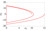
Figure 1: A motion plan to the sample motion planning problem for actuated bouncing ball system.

The flow is allowed when the ball is above the surface. Hence, the flow set is $C:=\{(x,u)\in\mathbb{R}^{2}\times\mathbb{R}:x_{1}\geq 0\}.$ At every impact, the velocity of the ball changes from pointing down to pointing up while the height remains the same. The dynamics at jumps of the actuated bouncing ball system is given as $x^{+}=\left[\begin{matrix}x_{1}\\ -\lambda x_{2}+u\end{matrix}\right]=:g(x,u),(x,u)\in D$ where $u\geq 0$ is the input and $\lambda\in(0,1)$ is the coefficient of restitution. The jump is allowed when the ball is on the surface with negative velocity. Hence, the jump set is $D:=\{(x,u)\in\mathbb{R}^{2}\times\mathbb{R}:x_{1}=0,x_{2}\leq 0,u\geq 0\}.$

Given the initial state set $X_{0}=\{(15,0)\}$, the final state set $X_{f}=\{(10,0)\}$, and the unsafe set $X_{u}=\{(x,u)\in\mathbb{R}^{2}\times\mathbb{R}:x_{1}\in[20,\infty),u\in[5,\infty)\}$, an instance of the optimal motion planning problem for the actuated bouncing ball system is to find a motion plan that has minimal hybrid time. To capture the hybrid time domain information, an auxiliary state $\tau\in\mathbb{R}_{\geq 0}$ representing the normal time and an auxiliary state $k\in\mathbb{N}$ representing the jump numbers are imported. An auxiliary hybrid system $\overline{\mathcal{H}}:=(\overline{C},\overline{f},\overline{D},\overline{g})$ with state $\overline{x}:=(x,\tau,k)\in\mathbb{R}^{2}\times\mathbb{R}_{\geq 0}\times\mathbb{N}$ is constructed as follows

1. $\overline{C}:=\left\{(\overline{x},u)\in\mathbb{R}^{2}\times\mathbb{R}_{\geq 0}\times\mathbb{N}\times\mathbb{R}:(x,u)\in C\right\}$;

2. $\overline{f}(\overline{x},u):=\left[\begin{matrix}f(x,u)\\ 1\\ 0\end{matrix}\right],(\overline{x},u)\in\overline{C}$;

3. $\overline{D}:=\left\{(\overline{x},u)\in\mathbb{R}^{2}\times\mathbb{R}_{\geq 0}\times\mathbb{N}\times\mathbb{R}:(x,u)\in D\right\}$;

4. $\overline{g}(\overline{x},u):=\left[\begin{matrix}g(x,u)\\ \tau\\ k+1\end{matrix}\right],(\overline{x},u)\in\overline{D}$.

with the $X_{0}$, $X_{f}$, and $X_{u}$ extended to

1. $\overline{X}_{0}:=X_{0}\times(0,0)$;

2. $\overline{X}_{f}:=X_{f}\times\mathbb{R}_{\geq 0}\times\mathbb{N}$;

3. $\overline{X}_{u}:=X_{u}\times\mathbb{R}_{\geq 0}\times\mathbb{N}$.

Then the cost functional $c$ can be defined as

$$c(\overline{\phi})=c(\phi,\tau,k):=\tau(T,J)+k(T,J)$$ (2)

where $\overline{\phi}=(\phi,\tau,k)$ denotes a state trajectory of the solution pair to $\overline{\mathcal{H}}$, and $(T,J)=\max\mathop{\rm dom}\nolimits\overline{\phi}$. Then the example optimal motion planning problem for the bouncing ball is defined as $\mathcal{P}^{*}=(\overline{X}_{0},\overline{X}_{f},\overline{X}_{u},(\overline{C},\overline{f},\overline{D},\overline{g}),c)$

Example III.2

(Collision-resilient tensegrity multicopter system [14]) Consider a collision-resilient tensegrity multicopter in horizontal plane that can operate after colliding with a concrete wall. The state of the multicopter is composed of the position vector $p:=(p_{x},p_{y})\in\mathbb{R}^{2}$, where $p_{x}$ denotes the position along $x$-axle and $p_{y}$ denotes the position along $y$-axle, the velocity vector $v:=(v_{x},v_{y})\in\mathbb{R}^{2}$, where $v_{x}$ denotes the velocity along $x$-axle and $v_{y}$ denotes the velocity along $y$-axle, and the acceleration vector $a:=(a_{x},a_{y})\in\mathbb{R}^{2}$ where $a_{x}$ denotes the acceleration along $x$-axle and $a_{y}$ denotes the acceleration along $y$-axle. The state of the system is $x:=(p,v,a)\in\mathbb{R}^{6}$ and its input is $u:=(u_{x},u_{y})\in\mathbb{R}^{2}$.

The environment is assumed to be known. Define the region of the walls as $\mathcal{W}\subset\mathbb{R}^{2}$, represented by blue rectangles in Figure 3. Flow is allowed when the multicopter is in the free space. Hence, the flow set is $C:=\{((p,v,a),u)\in\mathbb{R}^{6}\times\mathbb{R}^{2}:p\notin\cal W\}.$ The dynamics of the quadrotors when no collision occurs can be captured using time-parameterized polynomial trajectories because of its differential flatness as $\dot{x}=\left[\begin{matrix}v\\ a\\ u\end{matrix}\right]=:f(x,u),(x,u)\in C;$ see [15].

Note that the post-collision position stays the same as the pre-collision position. Therefore, $p^{+}=p.$ Denote the velocity component of $v=(v_{x},v_{y})$ that is normal to the wall as $v_{n}$ and the velocity component that is tangential to the wall as $v_{t}$. Then, the velocity component $v_{n}$ after the jump is modeled as$v_{n}^{+}=-ev_{n}=:g^{v}_{n}(v)$ where $e\in(0,1)$ is the coefficient of restitution. The velocity component $v_{t}$ after the jump is modeled as $v_{t}^{+}=v_{t}+\kappa(-e-1)\arctan\frac{v_{t}}{v_{n}}v_{n}=:g^{v}_{t}(v)$ where $\kappa\in\mathbb{R}$ is a constant; see [14]. Denote the projection of the updated vector $(v^{+}_{n},v^{+}_{t})$ onto $x$ axle as $\Pi_{x}(v^{+}_{n},v^{+}_{t})$ and the projection of the updated vector $(v^{+}_{n},v^{+}_{t})$ onto $y$ axle as $\Pi_{y}(v^{+}_{n},v^{+}_{t})$. Therefore,

$$v^{+}=\left[\begin{matrix}\Pi_{x}(g^{v}_{n}(v),g^{v}_{t}(v))\\ \Pi_{y}(g^{v}_{n}(v),g^{v}_{t}(v))\end{matrix}\right]=:g^{v}(v).$$

We assume that $a^{+}=0$, which corresponds to a hovering status. The discrete dynamics capturing the collision process is modeled as $x^{+}=\left[\begin{matrix}p\\ g^{v}(v)\\ 0\end{matrix}\right]=:g(x,u),(x,u)\in D.$ The jump is allowed when the multicopter is on the wall surface with positive velocity towards the wall. Hence, the jump set is $D:=\{((p,v,a),u)\in\mathbb{R}^{6}\times\mathbb{R}^{2}:p\in\partial\mathcal{W},v_{n}<0\}.$

Given the initial state set as $X_{0}=\{(1,2,0,0,0,0)\}$, the final state set as $X_{f}=\{(5,4)\}\times\mathbb{R}^{4}$, and the unsafe set as $X_{u}=\{(x,u)\in{\mathbb{R}^{6}\times\mathbb{R}^{2}}:p_{x}\in(\infty,0]\cup[6,\infty),p_{y}\in(\infty,0]\cup[5,\infty),(p_{x},p_{y})\in\operatorname{int}{\cal W}\}$, an instance of the optimal motion planning problem for the collision-resilient tensegrity multicopter system is to find the motion plan with minimal hybrid time as Example III.1.

IV HySST: An Optimal Motion Planning Algorithm for Hybrid Systems

IV-A Overview

In this paper, we propose an SST algorithm for hybrid systems, which we refer to as HySST algorithm. HySST algorithm searches for the optimal motion plan by incrementally constructing a search tree. The search tree is modeled by a directed tree. A directed tree is a pair $\mathcal{T}=(V,E)$, where $V$ is a set whose elements are called vertices and $E$ is a set of paired vertices whose elements are called edges. The edges in a directed tree are directed, which means the pairs of vertices that represent edges are ordered. The set of edges $E$ is defined as $E\subset\{(v_{1},v_{2}):v_{1}\in V,v_{2}\in V,v_{1}\neq v_{2}\}$. The edge $e=(v_{1},v_{2})\in E$ represents an edge from $v_{1}$ to $v_{2}$. A path in $\mathcal{T}$ is a sequence of vertices $p=(v_{1},v_{2},...,v_{k})$ such that $(v_{i},v_{i+1})\in E$ for all $i\in\{1,2,...,k-1\}$. If there exists a path from the vertex $v_{0}$ to the vertex $v_{1}$ in the search tree, then $v_{0}$ is called a parent vertex of $v_{1}$ and $v_{1}$ is called a child vertex of $v_{0}$.

Each vertex in the search tree is associated with a state value of $\mathcal{H}$ and a cost value that estimates the cost from the root vertex up to the vertex. Each edge in the search tree is associated with a solution pair to $\mathcal{H}$ that connects the state values associated with their endpoint vertices. The state value and the cost value associated with vertex $v\in V$ is denoted as $\overline{x}_{v}$ and $\overline{c}_{v}$, respectively. The solution pair associated with edge $e\in E$ is denoted as $\overline{\psi}_{e}$. The solution pair that the path $p=(v_{1},v_{2},...,v_{k})$ represents is the concatenation of all those solutions associated with the edges therein, namely,

$$\tilde{\psi}_{p}:=\overline{\psi}_{(v_{1},v_{2})}|\overline{\psi}_{(v_{2},v_{3})}|\ ...\ |\overline{\psi}_{(v_{k-1},v_{k})}$$ (3)

where $\tilde{\psi}_{p}$ denotes the solution pair associated with the path $p$. For the notion of concatenation, see Definition II.2.

HySST requires a library of possible inputs. The input library $(\mathcal{U}_{C},\mathcal{U}_{D})$ includes the input signals that can be applied during flows (collected in $\mathcal{U}_{C}$) and the input values that can be applied at jumps (collected in $\mathcal{U}_{D}$).

HySST employs a pruning process to decrease the number of vertices in the search tree. This pruning operation is implemented by maintaining a witness state set, denoted as $S$, such that all the vertices within the vicinity of the witnesses are ignored except the one with lowest cost. For every witness $s$ kept in $S$, a single vertex in the tree represents that witness. Such a vertex is stored in $s.rep$ for each witness $s\in S$.

HySST selects the vertex associated with the lowest cost within the vicinity of a randomly selected state. This vicinity of the randomly selected state, which we refer to as random state neighborhood, is defined by a ball of radius $\delta_{BN}\in\mathbb{R}_{>0}$. The pruning process removes from the search tree all the vertices within the vicinity of the closest witness to those removed vertices, which we refer to as closest witness neighborhood and is defined by a ball of radius $\delta_{s}\in\mathbb{R}_{>0}$, The pruning process does not remove the vertices in the closest witness neighborhood with lowest cost. Note that a vertex, say, $v_{a}$, may be associated to a higher cost than the costs associated with other vertices within the closest witness neighborhood of $v_{a}$, but has a child vertex, say, $v_{b}$, associated to the lowest cost compared with the costs of other vertices in the closest witness neighborhood of $v_{b}$. In this case, $v_{a}$ should not be removed from the search tree because if it is removed, $v_{b}$ is also removed due to being cascaded. However, even $v_{a}$ is not removed, it will not be selected, and, therefore, will be kept in a separate set called inactive vertex set, denoted $V_{inactive}$. On the other hand, the vertices that are not pruned are stored in a set called the active vertex set, denoted $V_{active}$.

Next, we introduce the main steps executed by HySST. Given the optimal motion planning problem $\mathcal{P}^{*}=(X_{0},X_{f},X_{u},(C,f,D,g),c)$ and the input library $(\mathcal{U}_{C},\mathcal{U}_{D})$, HySST performs the following steps:

1. Sample a finite number of points from $X_{0}$ and initialize a search tree $\mathcal{T}=(V,E)$ by adding vertices associated with each sampling point and setting $E$ as $E\leftarrow\emptyset$.

2. Initialize the witness state set $S\subset\mathbb{R}^{n}$ by $S\leftarrow\emptyset$. For each $v\in V$ such that for all $v^{\prime}\in V\backslash v$, $|\overline{x}_{v}-\overline{x}_{v^{\prime}}|>\delta_{s}$, add the witness state $s=\overline{x}_{v}$ to $S$ and set the representative of $s$ as $s.rep\leftarrow v$. Initialize the active vertices set $V_{active}$ by $V_{active}\leftarrow\{s.rep\in V:s\in S\}$. Initialize the inactive vertices set $V_{inactive}$ by $V_{inactive}\leftarrow\emptyset$.

3. Randomly select one regime among flow regime and jump regime for the evolution of $\mathcal{H}$.

4. Randomly select a point $x_{rand}$ from $C^{\prime}$ ($D^{\prime}$) if the flow (jump, respectively) regime is selected in Step 3.

5. Find all the vertices in $V_{active}$ associated with the state values that are within $\delta_{BN}$ to $x_{rand}$ and collect them in the set $V_{BN}$. Then, find the vertex in $V_{BN}$ that has minimal cost, denoted $v_{cur}$. If no vertex is collected in $V_{BN}$, then find the vertex in the search tree that has minimal distance to $x_{rand}$ and assign it to $v_{cur}$.

6. Randomly select an input signal (value) from $\mathcal{U}_{C}$ ($\mathcal{U}_{D}$) if $\overline{x}_{v_{cur}}\in C^{\prime}\backslash D^{\prime}$ ($\overline{x}_{v_{cur}}\in D^{\prime}\backslash C^{\prime}$). Then, compute a solution pair denoted $\psi_{new}=(\phi_{new},u_{new})$ starting from $\overline{x}_{v_{cur}}$ with the selected input applied via flow (jump, respectively). If $\overline{x}_{v_{cur}}\in D^{\prime}\cap C^{\prime}$, a random process is employed to decide to proceed the computation with flow or jump. Denote the final state of $\phi_{new}$ as $x_{new}$. Compute the cost at $x_{new}$, denoted $c_{new}$, by $c_{new}\leftarrow\overline{c}_{v_{cur}}+c(\phi_{new})$. If $\psi_{new}$ does not intersect with $X_{u}$, then go to next step. Otherwise, go to Step 3.

7. Find one of the witnesses in $S$ that has minimal distance to $x_{new}$, denoted $s_{near}$, and proceed as follows:

   • If $|s_{near}-x_{new}|>\delta_{s}$, then add a new witness $s_{new}=x_{new}$ to $S$ and set its representative as $x_{new}$. Add a vertex $v_{new}$ associated with $x_{new}$ to $V_{active}$ and an edge $(v_{cur},v_{new})$ associated with $\psi_{new}$ to $E$. Then, go to Step 3.

   • If $|s_{near}-x_{new}|\leq\delta_{s}$,

     • if $\overline{c}_{s_{near}.rep}>c_{new}$, add a vertex $v_{new}$ associated with $x_{new}$ to $V_{active}$ and an edge $(v_{cur},v_{new})$ associated with $\psi_{new}$ to $E$. Then, update the representative of $s_{near}$ by the newly added vertex, i.e., $s_{near}.rep\leftarrow v_{new}$, and prune the vertex, say, $v_{pre\_near}$ which is previously witnessed by $s_{near}$. If $v_{pre\_near}$ is an inactive vertex, i.e., is such as $v_{a}$ described above, then add $v_{pre\_near}$ to $V_{inactive}$. Otherwise, remove $v_{pre\_near}$ and all its child vertices from the search tree. Then, go to Step 3.

     • if $\overline{c}_{s_{near}.rep}\leq c_{new}$, go to Step 3 directly.

IV-B HySST Algorithm

Following the overview above, the proposed algorithm is given in Algorithm 1. The inputs of Algorithm 1 are the problem $\mathcal{P}^{*}=(X_{0},X_{f},X_{u},(C,f,D,g),c)$, the input library $(\mathcal{U}_{C},\mathcal{U}_{D})$, a parameter $p_{n}\in(0,1)$, which tunes the probability of proceeding with the flow regime or the jump regime, an upper bound $K\in\mathbb{N}_{>0}$ for the number of iterations to execute, and two tunable sets $X_{c}\supset\overline{C^{\prime}}$ and $X_{d}\supset D^{\prime}$, which act as constraints in finding a closest vertex to $x_{rand}$. In addition, HySST requires additional parameters $\delta_{BN}$ and $\delta_{s}$ to tune the radius of random state neighborhood and closest witness neighborhood, respectively.

Algorithm 1 HySST algorithm

Input: $X_{0},X_{f},X_{u},\mathcal{H}=(C,f,D,g),(\mathcal{U}_{C},\mathcal{U}_{D}),p_{n}\in(0,1)$, $K\in\mathbb{N}_{>0}$, $X_{c}$, $X_{d}$, $\delta_{BN}$ and $\delta_{s}$

1:$\mathcal{T}.init(X_{0})$;

2:$V_{active}\leftarrow V$, $V_{inactive}\leftarrow\emptyset$, $S\leftarrow\emptyset$;

3:for all $v_{0}\in V$ do

4:    if $is\_vertex\_locally\_the\_best(\overline{x}_{v_{0}},0,S,\delta_{s})$ then

5:        $(S,$ $V_{active},$ $V_{inactive},$$E)\leftarrow prune\_dominated\_vertices(v_{0},S,V_{active},V_{inactive},E)$

6:    end if

7:end for

8:for $k=1$ to $K$ do

9:    randomly select a real number $r$ from $[0,1]$;

10:    if $r\leq p_{n}$ then

11:        $x_{rand}\leftarrow random\_state(\overline{C^{\prime}})$;

12:        $v_{cur}$$\leftarrow$ $best\_near\_selection$$(x_{rand},\;$$V_{active},$$\delta_{BN},$$X_{c})$;

13:    else

14:        $x_{rand}\leftarrow random\_state(D^{\prime})$;

15:        $v_{cur}\leftarrow best\_near\_selection(x_{rand},V_{active},\delta_{BN},X_{d})$;

16:    end if

17:    $(is\_a\_new\_vertex\_generated,x_{new},\psi_{new},cost_{new})\leftarrow new\_state(v_{cur},(\mathcal{U}_{C},\mathcal{U}_{D}),\mathcal{H},X_{u})$

18:    if $is\_a\_new\_vertex\_generated$ & $is\_vertex\_locally\_the\_best(x_{new},cost_{new},S,\delta_{s})$ then

19:        $v_{new}\leftarrow V_{active}.add\_vertex(x_{new},cost_{new})$;

20:        $E.add\_edge(v_{cur},v_{new},\psi_{new})$;

21:        $(S,V_{active},V_{inactive},E)\leftarrow prune\_dominated\_vertices(v_{new},S,V_{active},V_{inactive},E)$;

22:    end if

23:end for

24:return $\mathcal{T}$;

Each function in Algorithm 1 is defined next.

IV-B1 $\mathcal{T}.init(X_{0})$

The function call $\mathcal{T}.init$ is used to initialize a search tree $\mathcal{T}=(V,E)$. It randomly selects a finite number of points from $X_{0}$. For each sampling point $x_{0}$, a vertex $v_{0}$ associated with $x_{0}$ is added to $V$. At this step, no edge is added to $E$.

IV-B2 $return\leftarrow is\_vertex\_locally\_the\_best(x,cost,S,\delta_{s})$

The function call $is\_vertex\_locally\_the\_best$ describes the conditions under which the state $x$ is considered for addition to the search tree as is shown in Algorithm 2. First, Algorithm 2 looks for the closest witness $s_{new}$ to $x$ from the witness set $S$ (line 1). If the closest witness is more than $\delta_{s}$ from $x$, then a new witness is added to $S$ (lines 2 - 6). If $s_{new}$ is just added as a witness or $cost$ is less than the cost of the closest witness’s representative (line 7), then the state $x$ with the cost $cost$ is locally optimal and a $true$ signal is returned (line 8). Otherwise, a $false$ signal is returned.

Algorithm 2 $is\_vertex\_locally\_the\_best(x,cost,S,\delta_{s})$

1:$s_{new}\leftarrow nearest(S,x)$;

2:if $|x-s_{new}|>\delta_{s}$ then

3:    $s_{new}\leftarrow x$

4:    $s_{new}.rep\leftarrow NULL$

5:    $S\leftarrow S\cup\{s_{new}\}$;

6:end if

7:if $s_{new}.rep==NULL$ or $cost<\overline{c}_{s_{new}.rep}$ then

8:    return true;

9:end if

10:return false;

IV-B3 $(S,V_{active},V_{inactive},E)\leftarrow prune\_dominated\_vertices(v,S,V_{active},V_{inactive},E)$

Algorithm 3 describes the pruning process of dominated vertices. First, Algorithm 3 looks for the witness $s_{new}$ that is closest to $\overline{x}_{v}$ and its representative $v_{peer}$ (lines 1 - 2). The previous representative, which is dominated by $v$ in terms of cost, is removed from the active set of vertices $V_{active}$ and is added to the inactive vertices set $V_{inactive}$ (lines 4 - 5). Then, $v$ replaces $v_{peer}$ as the representative of $s_{new}$ (line 7). If $v_{peer}$ is a leaf vertex, then it can also safely be removed from the search tree (lines 8 - 13). The removal of $v_{peer}$ may cause a cascading effect for its parents, if they have already been in the inactive set $V_{inactive}$ and the only reason they were maintained in the search tree was because they were leading to $v_{peer}$. Here, the function call $isleaf(v_{peer})$ returns $true$ signal if $v_{peer}$ is a leaf vertex, which means $v_{peer}$ does not have child vertices (line 8). The function call $parent(v_{peer})$ returns the parent vertex of $v_{peer}$ (line 9).

Algorithm 3 $(S,V_{active},V_{inactive},E)\leftarrow prune\_dominated\_vertices(v,S,V_{active},V_{inactive},E)$

1:$s_{new}\leftarrow nearest(S,\overline{x}_{v})$;

2:$v_{peer}\leftarrow s_{new}.rep$;

3:if $v_{peer}!=NULL$ then

4:    $V_{active}\leftarrow V_{active}\backslash\{v_{peer}\}$;

5:    $V_{inactive}\leftarrow V_{inactive}\cup\{v_{peer}\}$;

6:end if

7:$s_{new}.rep\leftarrow v$;

8:while $isleaf(v_{peer})$ and $v_{peer}\in V_{inactive}$ do

9:    $v_{parent}\leftarrow parent(v_{peer})$;

10:    $E\leftarrow E\backslash\{(v_{parent},v_{peer})\}$;

11:    $V_{inactive}\leftarrow V_{inactive}\backslash{v_{peer}}$;

12:    $v_{peer}\leftarrow v_{parent}$;

13:end while

IV-B4 $x_{rand}$$\leftarrow$$random\_state(S)$

The function call $random\_state$ randomly selects a point from the set $S\subset\mathbb{R}^{n}$. It is designed to select from $\overline{C^{\prime}}$ and $D^{\prime}$ separately depending on the value of $r$ rather than to select from $\overline{C^{\prime}}\cup D^{\prime}$. The reason is that if $\overline{C^{\prime}}$ ($D^{\prime}$) has zero measure while $D^{\prime}$ ($\overline{C^{\prime}}$) does not, the probability that the point selected from $\overline{C^{\prime}}\cup D^{\prime}$ lies in $\overline{C^{\prime}}$ ($D^{\prime}$, respectively) is zero, which would prevent finding a solution when one exists.

IV-B5 $v_{cur}\leftarrow best\_near\_selection(x_{rand},V_{active},\delta_{BN},X_{\star})$

The function call $best\_near\_selection$ searches for a vertex $v_{cur}$ in the active vertex set $V_{active}$ such that its associated state value is in the intersection between the set $X_{\star}$ and $x_{rand}+\delta_{BN}\mathbb{B}$, and has minimal cost where $\star$ is either $c$ or $d$. This function is implemented by solving the following optimization problem.

Problem 3

Given $x_{rand}\in\mathbb{R}^{n}$, a radius $\delta_{BN}>0$ of the random state neighborhood, a tunable state constraint set $X_{\star}$, and an active vertex set $V_{active}$, solve

$$\operatorname*{arg\,min}_{v\in V_{active}} \quad\overline{c}_{v}$$

s.t. $$\quad|\overline{x}_{v}-x_{rand}|\leq\delta_{BN}$$

$$\quad\overline{x}_{v}\in X_{\star}.$$

The data of Problem 3 comes from the arguments of the $best\_near\_selection$ function call. This optimization problem can be solved by traversing all the vertices in $V_{active}$.

IV-B6 $(is\_a\_new\_vertex\_generated,x_{new},\psi_{new},cost_{new})\leftarrow new\_state(v_{cur},(\mathcal{U}_{C},\mathcal{U}_{D}),\mathcal{H},X_{u})$

If $\overline{x}_{v_{cur}}\in\overline{C^{\prime}}\backslash D^{\prime}$ ($\overline{x}_{v_{cur}}$$\in$$D^{\prime}\backslash\overline{C^{\prime}}$), the function call $new\_state$ generates a new solution pair $\psi_{new}$ to hybrid system $\mathcal{H}$ starting from $\overline{x}_{v_{cur}}$ by applying a input signal $\tilde{u}$ (an input value $u_{D}$) randomly selected from $\mathcal{U}_{C}$ ($\mathcal{U}_{D}$, respectively). If $\overline{x}_{v_{cur}}$$\in\overline{C^{\prime}}\cap D^{\prime}$, then this function generates $\psi_{new}$ by randomly selecting flows or jump. The final state of $\psi_{new}=(\phi_{new},u_{new})$ is denoted as $x_{new}$. The cost $cost_{new}$ at $x_{new}$ is computed by $cost_{new}\leftarrow\overline{c}_{v_{cur}}+c(\phi_{new})$.

After $\psi_{new}$ and $x_{new}$ are generated, the function $new\_state$ checks if there exists $(t,j)\in\mathop{\rm dom}\nolimits\psi_{new}$ such that $\psi_{new}(t,j)\in X_{u}$. If so, then $\psi_{new}$ intersects with the unsafe set and $is\_a\_new\_vertex\_generated\leftarrow false$. Otherwise, this function returns $is\_a\_new\_vertex\_generated\leftarrow true$.

IV-B7 $v_{new}\leftarrow V_{active}.add\_vertex(x_{new},cost_{new})$ and $E.add\_edge$$(v_{cur}$, $v_{new}$, $\psi_{new})$

The function call $V_{active}.add\_vertex(x_{new},cost_{new})$ adds a new vertex $v_{new}$ to $V_{active}$ such that $\overline{x}_{v_{new}}\leftarrow x_{new}$ and $\overline{c}_{v_{new}}\leftarrow cost_{new}$ and returns $v_{new}$. The function call $E.add\_edge(v_{cur},v_{new},\psi_{new})$ adds a new edge $e_{new}=(v_{cur},v_{new})$ associated with $\psi_{new}$ to $E$.

IV-C Solution Checking during HySST Construction

At each iteration, when a new vertex and a new edge are added to the search tree, i.e., $is\_a\_new\_vertex\_generated==true$, a solution checking function is employed to check if a path in $\mathcal{T}$ can be used to construct a motion plan to the given motion planning problem. If this function finds a path $p=((v_{0},v_{1}),(v_{1},v_{2}),...,(v_{n-1},v_{n}))=:(e_{0},e_{1},...,e_{n-1})$ in $\mathcal{T}$ such that 1) $\overline{x}_{v_{0}}\in X_{0}$ and 2) $\overline{x}_{v_{n}}\in X_{f}$, then the solution pair $\tilde{\psi}_{p}$, defined in (3), is a motion plan to the given motion planning problem.

V Asymptotic Near-optimality Analysis

This section analyzes the asymptotic optimality property of HySST algorithm. The following assumption assumes that the cost functional is Lipchitz continuous along the purely continuous solution pairs, locally bounded at jumps, and also satisfies additivity, monotonicity, and non-degeneracy.

Assumption V.1

The cost functional $c:\Sigma_{\phi}\to\mathbb{R}_{\geq 0}$ satisfies the following:

1. It is Lipschitz continuous for all continuous solution pairs $(\phi_{0},u_{0})$ and $(\phi_{1},u_{1})$ such that $\phi_{0}(0,0)=\phi_{1}(0,0)$; specifically, there exists $K_{c}>0$ such that $|c(\phi_{0})-c(\phi_{1})|\leq K_{c}\sup_{(t,0)\in\mathop{\rm dom}\nolimits\phi_{0}\cap\mathop{\rm dom}\nolimits\phi_{1}}\{|\phi_{0}(t,0)-\phi_{1}(t,0)|\}$.

2. For each purely discrete solution pairs $(\phi_{0},u_{0})$ and $(\phi_{1},u_{1})$ with one jump such that $\mathop{\rm dom}\nolimits\phi_{0}=\mathop{\rm dom}\nolimits\phi_{1}=\{0\}\times\{0,1\}$ and $\phi_{0}(0,0)=\phi_{1}(0,0)$, there exists $K_{d}>0$ such that $|c(\phi_{0})-c(\phi_{1})|\leq K_{d}\sup_{j\in\{0,1\}}\{|\phi_{0}(0,j)-\phi_{1}(0,j)|\}$.

3. Consider two solution pair $\psi_{0}=(\phi_{0},u_{0})$ and $\psi_{1}=(\phi_{1},u_{1})$ such that their concatenation is $\psi_{0}|\psi_{1}$. The following hold:

   1. $c(\phi_{0}|\phi_{1})=c(\phi_{0})+c(\phi_{1})$ (additivity);

   2. $c(\phi_{1})\leq c(\phi_{0}|\phi_{1})$ (monotonicity);

   3. For each $t_{2}>t_{1}\geq 0$ such that $(t_{1},j)\in\mathop{\rm dom}\nolimits\psi_{0}$ and $(t_{2},j)\in\mathop{\rm dom}\nolimits\psi_{0}$ for some $j\in\mathbb{N}$, there exists $M_{c}>0$ such that $t_{2}-t_{1}\leq M_{c}|c(\phi_{0}(t_{2},j))-c(\phi_{0}(t_{1},j))|$ (non-degeneracy during flows).

   4. For each $j_{1},j_{2}\in\mathbb{N}$ such that $j_{2}>j_{1}$, $(t,j_{1})\in\mathop{\rm dom}\nolimits\psi_{0}$ and $(t,j_{2})\in\mathop{\rm dom}\nolimits\psi_{0}$ for some $t\in\mathbb{R}_{\geq 0}$, there exists $M_{d}>0$ such that $j_{2}-j_{1}\leq M_{d}|c(\phi_{0}(t,j_{2}))-c(\psi_{0}(t,j_{1}))|$ (non-degeneracy at jumps).

Remark V.2

Items 1) and 2) above guarantee that the cost of the nearby solution pairs are bounded by the distance between the solutions. Item 3) above guarantees that the cost of the solution pairs can be computed incrementally and that the global minimum of the cost functional can be found by the optimal motion planning problem.

Next we define the clearance of the potential motion plans, which is heavily used in the literature; see [16].

Definition V.3 (Safety clearance of a solution pair)

Given a motion plan $\psi=(\phi,u)$ to the optimal motion planning problem $\mathcal{P}^{*}=(X_{0},X_{f},X_{u},(C,f,D,g),c)$, the safety clearance $\delta_{s}$ of $\psi=(\phi,u)$ is equal to the maximal $\delta^{\prime}>0$ if the following hold:

1. $\phi(0,0)+\delta^{\prime}\mathbb{B}\subset X_{0}$;

2. For all $(t,j)\in\mathop{\rm dom}\nolimits\psi$, $(\phi(t,j)+\delta^{\prime}\mathbb{B},u(t,j)+\delta^{\prime}\mathbb{B})\cap X_{u}=\emptyset$.

3. $\phi(T,J)+\delta^{\prime}\mathbb{B}\subset X_{f}$, where $(T,J)=\max\mathop{\rm dom}\nolimits(\phi,u)$.

Assumption V.4

The optimal motion plan to the given optimal motion planning problem has positive safety clearance $\delta_{s}$.

Definition V.5 (Dynamics clearance of a solution pair)

Given a motion plan $\psi=(\phi,u)$ to the optimal motion planning problem $\mathcal{P}^{*}=(X_{0},X_{f},X_{u},(C,f,D,g),c)$, the dynamics clearance $\delta_{d}$ of $\psi=(\phi,u)$ is equal to the maximal $\delta^{\prime}>0$ satisfying the following:

1. For all $(t,j)\in\mathop{\rm dom}\nolimits\psi$ such that $I^{j}$ has nonempty interior, $(\phi(t,j)+\delta^{\prime}\mathbb{B},u(t,j)+\delta^{\prime}\mathbb{B})\subset C$;

2. For all $(t,j)\in\mathop{\rm dom}\nolimits\psi$ such that $(t,j+1)\in\mathop{\rm dom}\nolimits\psi$, $(\phi(t,j)+\delta^{\prime}\mathbb{B},u(t,j)+\delta^{\prime}\mathbb{B})\subset D$.

Assuming that the optimal motion plan has positive dynamics clearance is restrictive for hybrid systems. Indeed, if the motion plan reaches the boundary of the flow set or of the jump set, then the motion plan has no clearance. To overcome this issue, the $\delta_{f}$-inflation of hybrid systems, denoted $\mathcal{H}_{\delta_{f}}:=(C_{\delta_{f}},f_{\delta_{f}},D_{\delta_{f}},g_{\delta_{f}})$ for some $\delta_{f}>0$, in our previous work is employed to create a positive dynamics clearance; see [10]. With both safety clearance and dynamics clearance defined, we are ready to define the clearance of the solution pair.

Definition V.6 (Clearance of a solution pair)

Given a motion plan $\psi=(\phi,u)$ to the optimal motion planning problem $\mathcal{P}^{*}=(X_{0},X_{f},X_{u},(C,f,D,g),c)$, the clearance of $\psi=(\phi,u)$, denoted $\delta$, is defined as the minimum of its safety clearance $\delta_{s}$ and dynamics clearance $\delta_{d}$, i.e., $\delta:=\min\{\delta_{s},\delta_{d}\}$.

The following assumption relating the clearance $\delta$ of the optimal motion plan with the algorithm parameters $\delta_{BN}$ and $\delta_{s}$ is necessary to establish the optimality property.

Assumption V.7

Given the clearance $\delta$ of the optimal motion plan, the parameters $\delta_{BN}$ and $\delta_{s}$ need to satisfy the following relationship

$$\delta_{BN}+2\delta_{s}<\delta.$$

The following assumption is imposed on the input library.

Assumption V.8

The input library $(\mathcal{U}_{C},\mathcal{U}_{D})$ is such that

1. Each input signal in $\mathcal{U}_{C}$ is constant and $\mathcal{U}_{C}$ includes all possible input signals such that their time domains are subsets of the interval $[0,T_{m}]$ for some $T_{m}>0$ and their images belong to $U_{C}$. In other words, there exists $T_{m}>0$ such that $\mathcal{U}_{C}=\{\tilde{u}:\mathop{\rm dom}\nolimits\tilde{u}=[0,T]\subset[0,T_{m}],\tilde{u}\text{ is }\text{constant}\text{ and }\mathop{\rm rge}\tilde{u}\in U_{C}\}$;

2. $\mathcal{U}_{D}=U_{D}$.

The following assumption is imposed on the random selection in HySST.

Assumption V.9

The probability distributions of the random selection in the function calls $T.init$, $random\_state$, and $new\_state$ are the uniform distribution.

The following assumptions are imposed on the flow map $f$ and the jump map $g$ of the hybrid system $\mathcal{H}$ in (1).

Assumption V.10

The flow map $f$ is Lipschitz continuous. In particular, there exist $K^{f}_{x},K^{f}_{u}\in\mathbb{R}_{>0}$ such that, for all $(x_{0},x_{1},u_{0},u_{1})$ such that $(x_{0},u_{0})\in C$, $(x_{0},u_{1})\in C$, and $(x_{1},u_{0})\in C$,

$$|f(x_{0},u_{0})-f(x_{1},u_{0})| \leq K^{f}_{x}|x_{0}-x_{1}|$$

$$|f(x_{0},u_{0})-f(x_{0},u_{1})| \leq K^{f}_{u}|u_{0}-u_{1}|.$$

Assumption V.11

The jump map $g$ is such that there exist $K^{g}_{x}\in\mathbb{R}_{>0}$ and $K^{g}_{u}\in\mathbb{R}_{>0}$ such that, for all $(x_{0},u_{0})\in D$ and $(x_{1},u_{1})\in D$,

$$|g(x_{0},u_{0})-g(x_{1},u_{1})|\leq K^{g}_{x}|x_{0}-x_{1}|+K^{g}_{u}|u_{0}-u_{1}|.$$

Then, we are ready to provide our main result showing that by feeding the the inflation of the original hybrid system, HySST would find a solution such that the cost is close to the minimal cost regardless of the positive dynamics clearance. See [12] for a detailed proof.

Theorem V.12

Given an optimal motion planning problem $\mathcal{P}^{*}=(X_{0},X_{f},X_{u},(C,f,D,g),c)$, suppose Assumptions V.1, V.7, V.8, V.9, V.10, and V.11 are satisfied and that there exists an optimal motion plan $\psi^{*}=(\phi^{*},u^{*})$ to $\mathcal{P}^{*}$ satisfying Assumption V.4 for some $\delta_{s}>0$. When HySST is used to solve the motion planning problem $\mathcal{P}^{*}_{\delta_{f}}=(X_{0},X_{f},X_{u},(C_{\delta_{f}},f_{\delta_{f}},D_{\delta_{f}},g_{\delta_{f}}),c)$ where, for some $\delta_{f}>0$, $(C_{\delta_{f}},f_{\delta_{f}},D_{\delta_{f}},g_{\delta_{f}})$ denotes $\delta_{f}$-inflation of $(C,f,D,g)$, the probability that HySST finds a motion plan $\psi=(\phi,u)$ such that $c(\phi)\leq(1+\alpha\delta)c(\phi^{*})$ converges to one as the number of iterations $k$ goes to infinity for some constant ${\alpha}\geq 0$, where $\delta=\min\{\delta_{s},\delta_{f}\}$.

VI HySST Software Tool for Optimal Motion Planning Problems for Hybrid Systems

Algorithm 1 leads to a software tool to solve the optimal motion planning problems for hybrid systems. This software only requires the inputs listed in Algorithm 1. Next, HySST algorithm and this tool are illustrated in Examples III.1 and III.2.

Example VI.1

(Actuated bouncing ball system) The simulation result in Figure 2 shows that HySST is able to find a motion plan for the instance of optimal motion planning problem for the actuated bouncing ball system.

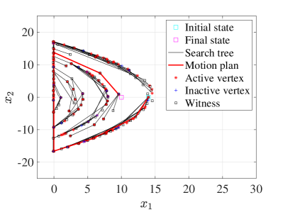
(a) HySST

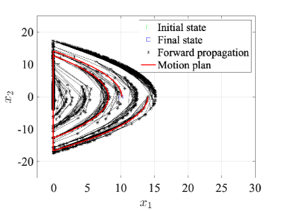
(b) HyRRT

Figure 2: Motion plans for actuated bouncing ball example solved by HySST and HyRRT in [10].

The simulation is implemented in MATLAB and processed by a $3.5$ GHz Intel Core i7 processor. Both HySST and HyRRT are run for $20$ times to solve the same problem. The HySST creates $154$ active vertices and $35$ inactive vertices and takes $3.30$ seconds, while HyRRT creates $660$ vertices in total and takes $18.4$ seconds on average. As is shown in Figure 2(a), only one jump occurs in the motion plans generated by HySST. Compared to the motion plans generated by HyRRT in Figure 2(b) where multiple jumps occur, the motion plan generated by HySST takes less hybrid time.

Example VI.2

(Collision-resilient tensegrity multicopter) The simulation result in Figure 3 shows that HySST is able to ultilize the collision with the wall to decrease the hybrid time of the motion plan for multicopter. This simulation is computed on the same computation platform as the previous example, and the simulation for this problem takes $54.7$ seconds and creates $2094$ active vertices on average.

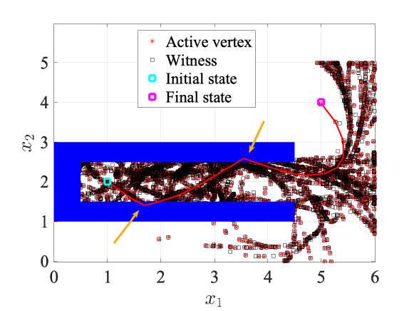
Figure 3: The motion plan generated by HySST for collision-resilient tensegrity multicopter. The blue rectangles denote the obstacles that may cause the collision with the multicopter. The yellow arrows point to the location where collision occurs.

VII Conclusion

In this paper, a HySST algorithm is proposed to solve optimal motion planning problems for hybrid systems. The proposed algorithm is illustrated in the bouncing ball and multicopter examples and the results show its capacity to solve the problem. In addition, this paper provides a result showing HySST algorithm is asymptotically near optimal under mild assumptions.

References

- [1] S. M. LaValle, Planning algorithms. Cambridge university press, 2006.
- [2] G. T. Wilfong, “Motion planning for an autonomous vehicle,” in Proceedings. 1988 IEEE International Conference on Robotics and Automation. IEEE, 1988, pp. 529–533.
- [3] O. Khatib, “Real-time obstacle avoidance for manipulators and mobile robots,” in Proceedings. 1985 IEEE international conference on robotics and automation, vol. 2. IEEE, 1985, pp. 500–505.
- [4] L. E. Kavraki, P. Svestka, J.-C. Latombe, and M. H. Overmars, “Probabilistic roadmaps for path planning in high-dimensional configuration spaces,” IEEE transactions on Robotics and Automation, vol. 12, no. 4, pp. 566–580, 1996.
- [5] S. M. LaValle and J. J. Kuffner Jr, “Randomized kinodynamic planning,” The international journal of robotics research, vol. 20, no. 5, pp. 378–400, 2001.
- [6] Y. Yang, J. Pan, and W. Wan, “Survey of optimal motion planning,” IET Cyber-Systems and Robotics, vol. 1, no. 1, pp. 13–19, 2019.
- [7] O. Nechushtan, B. Raveh, and D. Halperin, “Sampling-diagram automata: A tool for analyzing path quality in tree planners.” in WAFR. Springer, 2010, pp. 285–301.
- [8] S. Karaman and E. Frazzoli, “Sampling-based algorithms for optimal motion planning,” The international journal of robotics research, vol. 30, no. 7, pp. 846–894, 2011.
- [9] Y. Li, Z. Littlefield, and K. E. Bekris, “Asymptotically optimal sampling-based kinodynamic planning,” The International Journal of Robotics Research, vol. 35, no. 5, pp. 528–564, 2016.
- [10] N. Wang and R. G. Sanfelice, “A rapidly-exploring random trees motion planning algorithm for hybrid dynamical systems,” in 2022 IEEE 61st Conference on Decision and Control (CDC). IEEE, 2022, pp. 2626–2631.
- [11] R. G. Sanfelice, Hybrid feedback control. Princeton University Press, 2021.
- [12] N. Wang and R. G. Sanfelice, “Hysst: A stable sparse rapidly-exploring random trees optimal motion planning algorithm for hybrid dynamical systems,” University of California, Santa Cruz, Department of Electrical and Computer Engineering, Tech. Rep., 2023, password: hySST23. [Online]. Available: https://hybrid.soe.ucsc.edu/sites/default/files/preprints/TR-HSL-02-2023.pdf
- [13] R. G. Sanfelice, “Hybrid feedback control,” 2021.
- [14] J. Zha and M. W. Mueller, “Exploiting collisions for sampling-based multicopter motion planning,” in 2021 IEEE International Conference on Robotics and Automation (ICRA). IEEE, 2021, pp. 7943–7949.
- [15] S. Liu, N. Atanasov, K. Mohta, and V. Kumar, “Search-based motion planning for quadrotors using linear quadratic minimum time control,” in 2017 IEEE/RSJ international conference on intelligent robots and systems (IROS). IEEE, 2017, pp. 2872–2879.
- [16] M. Kleinbort, K. Solovey, Z. Littlefield, K. E. Bekris, and D. Halperin, “Probabilistic completeness of rrt for geometric and kinodynamic planning with forward propagation,” IEEE Robotics and Automation Letters, vol. 4, no. 2, pp. x–xvi, 2018.