Cosmological Constraints on CDM Models
Abstract
Problems with the concordance cosmology CDM as the cosmological constant problem, coincidence problems and Hubble tension has led to many proposed alternatives, as the CDM, where the now called cosmological term is allowed to vary due to an interaction with pressureless matter. Here, we analyze one class of these proposals, namely, , based on dimensional arguments. Using SNe Ia, cosmic chronometers data plus constraints on from SH0ES and Planck satellite, we constrain the free parameters of this class of models. By using the Planck prior over , we conclude that the term can not be discarded by this analysis, thereby disfavouring models only with the time-variable terms. The SH0ES prior over has an weak evidence in this direction. The subclasses of models with and with can not be discarded by this analysis. Finally, by using distance priors from CMB, the time-dependence was quite restricted.
I Introduction
The concordance cosmological model CDM ( plus Cold Dark Matter) is very successful in explaining a variety of cosmological observations as, for instance, the accelerating expansion of the Universe and the power spectrum of the cosmic microwave background radiation (CMB). However, the model suffers several theoretical and observational difficulties. Some remarkable examples are the cosmological constant problem, the coincidence problem, and the Hubble tension (see, e.g., Perivolaropoulos2022 for a review).
In the last decades, we have seen an increasing number of alternatives to the CDM model aiming to alleviate such difficulties. These alternatives range from the quest for dark energy models to extended theories of gravity. In this context, it is natural to investigate if is a function of the cosmic time .
Models with a time-varying or Vacuum-decay models have been conceived in different contexts. In several models, some ad hoc time dependence for is assumed. Some of the most common examples were addressed in Refs. Vishwakarma2001 ; Ahmet2018 (see Overduin1998 and references therein for a list of phenomenological decay laws of ). The functional form of can also be derived, for instance, by geometrical motivations Azri2012 ; Azri2017 or from Quantum Mechanical arguments Szydlowski2015 . The interaction of vacuum with matter has also been considered in different approaches and confronted with recent cosmological data (see, e.g., Benetti2019 ; Papagian2020 ; Benetti2021 ; Bruni2022 ).
A promising approach to overcome the puzzles of the CDM model is known as the ‘running vacuum model’ (RVM). It emerges when one uses the renormalization group approach of quantum field theory in curved spaces to renormalize the vacuum energy density. It is possible to show that vacuum energy density evolves as a series of powers of the Hubble function and its derivatives with respect to cosmic time: . The leading term of the expansion is constant, but the next-to-leading one evolves as . There are other terms in the expansion that can be relevant for the early Universe cosmology, but the term can affect the current evolution of the scale factor. Initially, the RVM was introduced in a semi-qualitative way through the renormalization group approach. Some of the first motivations of this model can be found, e.g., in the Refs. Shapiro2000 ; Babic2001 ; Shapiro2002 ; Shapiro2003 (see also Sola2013 for an old review on the subject). However, in recent years, the RVM was derived from a rigorous analysis within the Quantum Field Theory in curved spacetime. The derivation of the final form of RVM can be found in the Refs. Pulido2020 ; Pulido2022a ; Pulido2022b ; Pulido2023 (see Peracaula2022 for a review on recent theoretical developments). Moreover, such a class of models can be more favored than the CDM model when a fit with the cosmological observables is performed Sola2017 ; Peracaula2018 ; Tsiapi2019 ; Mavromatos2021 ; Peracaula2023 ; Peracaula2021 ; Peracaula2018b .
To answer the conundrum of why the cosmological constant is so small today, one could also propose models with , where is the scale factor and is a positive constant to be determined. From dimensional arguments by quantum cosmology, it is natural to choose Lopez1996 ; Chen1990 . Therefore, in this perspective, has the same decay behavior as the curvature term. Such an evolution of was first proposed by Özer and Taha Ozer1986 ; Ozer1987 as a way to solve the cosmological problems of the eighties decade.
On the other hand, following similar phenomenological arguments, in Ref. Carvalho1992 , the authors parametrized the time evolution of as the sum of a term proportional to to a term proportional to , i.e., the same term that emerges from the RVM. In the present article, we follow this approach, but we add a “bare” cosmological term . Specifically, we consider four models of a time-varying in the class
| (1) |
with , and constants. Three models are chosen by selecting one of these constants to vanish identically (these three models are depicted in Table 1) and the fourth model is the complete one for which the three constants are non-null.
The phenomenological model described by the complete model presents a smooth transition from the early de Sitter stage to the radiation phase. Such a transition is independent of the curvature parameter and solves naturally the horizon and the graceful exit problem Lima2015 .
To put constraints on the free parameters of the models, we use the SNe Ia sample consisting of 1048 SNe Ia apparent magnitude measurements from the Pantheon sample pantheon and a compilation of 32 cosmic chronometers data of the Hubble parameter, MorescoEtAl22 . We have also considered the most up-to-date constraints on , namely, the ones from SH0ES Riess2021 and Planck Planck2020 .
We organized the article as follows. We describe the Friedmann equations with a time-dependent -term in Section II (neglecting radiation) and Section III (including radiation). We obtain analytical solutions for in the class of models given by Eq. (1) in Sections II.1 and III.1. In Section IV, we constrain the parameters of the models using SNe Ia data, cosmic chronometers data and CMB. In the analysis, we consider separately the constraints on from Planck (Section IV.1) and from SH0ES (Section IV.2). Finally, we present our conclusions and final remarks in Section V.
II Cosmological equations for a varying term, neglecting radiation
From the Cosmological Principle and the Einstein Field Equations, we have the so-called Friedmann equations, given by
| (2) | ||||
| (3) |
where is the total density of the Universe matter-energy content, is total pressure and is the curvature scalar. As we are mainly interested in the late-time Universe, we shall neglect the radiation contribution, in such a way that is given by
| (4) |
where corresponds to the total pressureless matter (dark matter+baryons) and corresponds to the time-varying -term. In the present article we assume the equation of state (EoS) of vacuum to be exactly such that . However, a recent result for the RVM is that the EoS of vacuum evolves with the cosmic history Pulido2022b . This would change our results and may be considered in future works. From the continuity equation, we have
| (5) | ||||
| (6) |
where is the interaction term between pressureless matter and vacuum. With these components, the Friedmann equations (3) now read
| (7) | ||||
| (8) |
By multiplying the Eq. (8) by 2, we have
| (9) |
and summing the Eq. (7) with the Eq. (9), we have
| (10) |
Since , Eq. (10) reads
| (11) |
By replacing , we find
| (12) |
In order to perform cosmological constraints, let us now change to derivatives with respect to the redshift
| (13) |
Thus, the equation
| (14) |
now reads
| (15) |
and by replacing we have
| (16) |
If we further use the definition the above equation reads
| (17) |
From now on, we shall assume that the Universe is spatially flat (), as indicated by inflation and CMB. Therefore, we finally obtain the equation
| (18) |
For a given (or ), Eq. (18) can be solved in order to obtain the universe evolution . In the next subsection, we shall assume a fair general dependence in order to solve this equation and compare the assumed models with cosmological observations.
II.1 class of models, neglecting radiation
Dimensional arguments have led to the proposals of , models in the literature. Here we test a combination of these proposals together with a constant term, in order to find which of these terms may contribute the most to the evolution of the universe as indicated by observations. So, the models we study here are derived from the following dependence
| (19) |
We shall not consider this general as a model to be constrained by observations, as it has too many free parameters, and it may be penalized in a Bayesian criterion. Actually, we choose to work with particular cases of this dependence, where, in each case, one parameter contribution is neglected, as summarised in Table 1
| Model | Fixed parameter | |
|---|---|---|
Let us now obtain the evolution of this class of models. From Eq. (19), we have the values today
| (20) |
As , we may also write
| (21) |
where we have defined and the dimensionless , for mathematical convenience. From this, we may write for
| (22) |
As already mentioned, we choose to work with a spatially flat Universe, such that from Eq. (7), we have the normalization condition
| (23) |
Now, with these dimensionless parameters , an analytical solution for the Eq. (18) can be obtained. The general solution is given by
| (24) |
The solutions for each one of the three models depicted in the Table 1 are particular cases of this solution obtined by the appropriate choice of parameters. They are given by
-
•
Model , ()
(25) -
•
Model , ()
(26) -
•
Model , ()
(27)
It is worth noticing that, for the model, the given by Eq. (26) is similar to the CDM model with spatial curvature. This is due to the fact that the term mimics a curvature term in this case.
The functions we have obtained are all we need in order to constrain the three models with observational data in the next section. We can also obtain the interaction term for each model, in order to analyze its behavior later. For the general case (19), we have the following interaction term
| (28) |
III Cosmological Equations for a Varying Term, including radiation
Taking radiation into account, the Friedmann equations (3) are the same, but now we have and given by:
| (29) | ||||
| (30) |
where is radiation density and (dark matter ()+baryons ()). The continuity equations now read
| (31) | ||||
| (32) | ||||
| (33) | ||||
| (34) |
where is the interaction term between dark matter and vacuum. It is interesting to note that Eqs. (31) and (33) can be combined to write a continuity equation for total pressureless matter:
| (35) |
With these components, the Friedmann equations (3) now read
| (36) | ||||
| (37) |
It can be shown, that following the same steps as in Sec. II, we may arrive at the general result, with spatial curvature:
| (38) |
And, by assuming that the Universe is spatially flat (), as indicated by inflation and CMB, we obtain the equation:
| (39) |
For a given (or ), Eq. (39) can be solved in order to obtain the universe evolution . In the next subsection, we assume the same dependence as before (19) in order to solve this equation and compare the assumed models with cosmological observations.
III.1 class of models, including radiation
For this class, including radiation, the normalization condition now reads:
| (40) |
Now, with the dimensionless parameters , an analytical solution for the Eq. (18) can be obtained. The general solution is given by
| (41) |
which is a general solution in the cases that .
IV Analysis and Results
For this analysis, we use 3 variations of the general equation, being first with , second with , and last we take , as described in Tab. 1.
In order to constrain the models in the present work, we have used as observational data, the SNe Ia sample consisting of SNe Ia apparent magnitude measurements from the Pantheon sample pantheon and a compilation of Hubble parameter data, MorescoEtAl22 , obtained by estimating the differential ages of galaxies, called Cosmic Chronometers (CCs).
The 32 CCs data is a sample compiled by MorescoEtAl22 , consisting of data within the range . In the Ref. MorescoEtAl22 , the authors have estimated systematic errors for these data, by running simulations and considering effects such as metallicity, rejuvenation effect, star formation history, initial mass function, choice of stellar library etc.111The method to obtain the full covariance matrix, together with jupyter notebooks as examples are furnished by M. Moresco at https://gitlab.com/mmoresco/CCcovariance.
The Pantheon compilation consists of data from SNe Ia, within the redshift range , containing measurements of SDSS, Pan-STARRS1 (PS1), SDSS, SNLS, and various HST and low- datasets.
In order to better constrain the models, besides SNe Ia+ data, we have also considered the most up-to-date constraints over , namely, the ones from SH0ES km/s/Mpc Riess2021 and Planck km/s/Mpc Planck2020 . As it is well known, these constraints are currently in conflict, generating the so-called “ tension” H0TensionReview . It is important to mention that these constraints are obtained from quite different methods. While the SH0ES is obtained simply from local constraints, following the distance ladder built from Cepheid distances and local SNe Ia, the Planck is obtained from high redshift constraints, assuming the flat CDM model. Given this tension, we preferred to make two separate analyses, one considering the from Planck and one taking into account the from SH0ES.
Below, we show the results of our analyses, first showing the constraints from SNe Ia++ from Planck, and later showing the constraints from SNe Ia++ from SH0ES.
In all the analyses that we have made, we have assumed the flat priors over the free parameters: , , , km/s/Mpc. It is important to note that while SNe Ia data constrain , , , data constrain . However, data alone do not provide strong constraints over the free parameters, so we choose to work with +SNe Ia data combination. Furthermore, we have added constraints over from Planck and SH0ES in order to probe the tension and also because they consist of strong constraints over .
IV.1 SNe Ia++Planck analysis
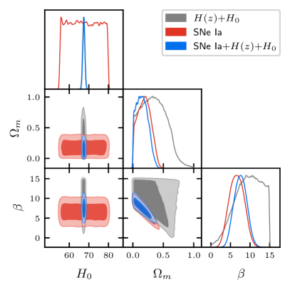
We start with the model (see Table 1). As one may see in Fig. 1 (left), is well constrained by +Planck data, but and are poorly constrained. In fact, one may see that is constrained by the prior in its inferior limit, while is constrained by the prior in its superior limit. can not be constrained by SNe Ia, but is well constrained by this data. is better constrained by SNe Ia, but also is constrained inferiorly by the prior. In Fig. 1 (right), we can see the result for the joint analysis, where and are better constrained, although yet is constrained inferiorly by the prior. We show the best-fit values for the parameters of the model in Table 2.
| Parameter | 95% limits |
|---|---|
| (km/s/Mpc) | |

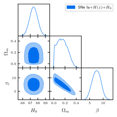
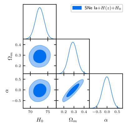
In Fig. 2 we show the analysis for the model (). As one can see in the left panel, +Planck data constrains well and , but not , which is constrained by the prior in its inferior limit. As SNe Ia does not constrain , but and are well constrained by this data, it is interesting to combine SNe Ia and data. One may see in Fig. 2 (Right) and Table 3, the result for the joint analysis, where , and are better constrained.
| Parameter | 95% limits |
|---|---|
| (km/s/Mpc) | |
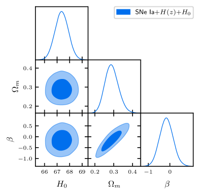
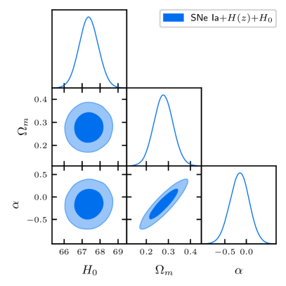
Next, we analyze the model () for which we also put constraints on the parameters . In Fig. 3 (Left), we can see that and are well constrained by +Planck data, while is weakly constrained. and are well constrained by SNe Ia, thus complementing the +Planck data constraints. In Fig. 3 (Right) and Table 4, we highlight the result for the joint analysis, where , , and are better constrained.
| Parameter | 95% limits |
|---|---|
| (km/s/Mpc) | |


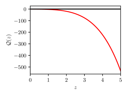
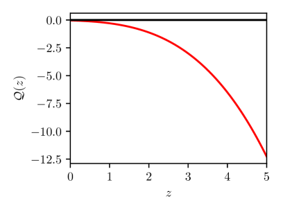
From Fig. 4 (upper panel), one may notice that in the past () the interaction term was positive, meaning a vacuum decaying into DM. However, it is interesting that, for this model (), the interaction term changes sign at low redshift, indicating that now we have decaying of DM into . This is due to the fact that and in the best fit, leading to a change of sign of , as one may see from Eq. (28). For and models, however, the interaction term is always negative, thus indicating a decaying of DM into . We may conclude that, at least for the best-fit models, that is the only model that alleviates or solves the Cosmological Constant Problem (CCP). However, as one can see from Tables II and III, and may have positive values within 95% c.l., thus allowing also for decaying of into DM. For , however, there is not such a change of tendency when we change the values of and within 95% c.l.
IV.2 SNe Ia++SH0ES analysis
In Fig. 5, we may see the constraints from SNe Ia, data and from SH0ES over the model (with ).
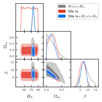
As one may see in Fig. 5 (left), +SH0ES data constrains well , but not , as it is being constrained by the prior in its inferior limit, while is constrained by the prior in its superior limit. is not constrained by SNe Ia, but and are better constrained by this data. In Fig. 5 (right), we can see the result for the joint analysis, where and are better constrained, although still is constrained by the prior in its inferior limit. The best-fit values for the model in this case are shown in Table 5
| Parameter | 95% limits |
|---|---|
| (km/s/Mpc) | |
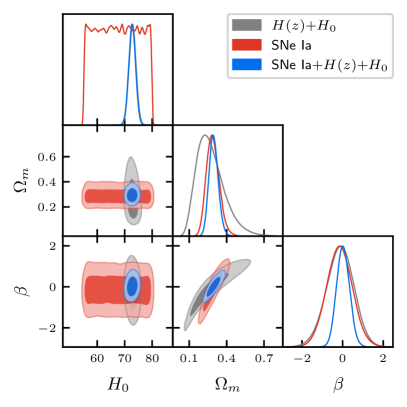
In Fig. 6, we may see the constraints from SNe Ia, data and from SH0ES over the model (with ).

In Fig. 6 (left), data constrains well and , but not , which is constrained by the prior in its inferior limit. is not constrained by SNe Ia, but and are well constrained by this data. In Fig. 6 (right) and in Table 6, we can see the result for the joint analysis, where and are better constrained. We may see that , and are well constrained by this analysis.
| Parameter | 95% limits |
|---|---|
| (km/s/Mpc) | |
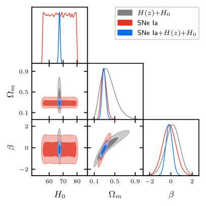
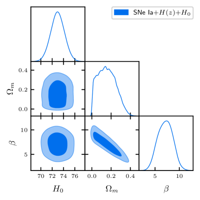
Below, in Fig. 7, we may see the constraints from SNe Ia, data and from SH0ES over the model (with ).
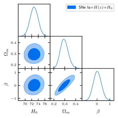
We can see in Fig. 7 (left), +SH0ES data constraints well and , but not , which is being constrained by the prior in its inferior limit. is not constrained by SNe Ia, but and are well constrained by this data. One may see in Fig. 7 (right), the result for the joint analysis, where , , and are well constrained. In Table 7 we show the best-fit values for this model.
| Parameter | 95% limits |
|---|---|
| (km/s/Mpc) | |
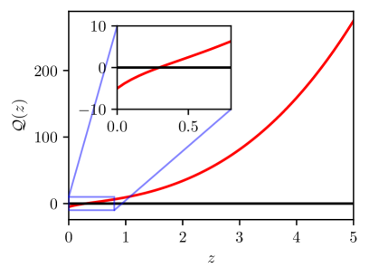
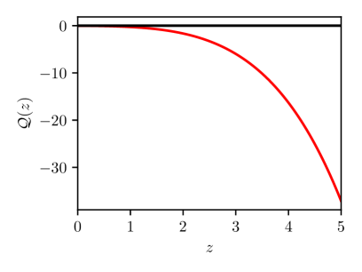
As one may see from Fig. 8, the interaction term has quite similar behavior to Fig. 4. That is, changes sign for the model and it is negative for models and , increasing its absolute value with redshift. However, the best-fit parameters from the analysis with the SH0ES prior indicate less interaction in the past than in the case with the Planck prior.
We can see from the figures above, that the most stringent constraints from the data are in the context of the model , followed by the constraints over the model . While the worst constraints over the parameters are in the case of the model . One reason for that is that, as one may see, the contours from SNe Ia and are misaligned in the cases and while being aligned in the case of . Then, we may say that in the context of the models, and , the SNe Ia and observations nicely complement each other.
Finally, in order to make a more quantitative comparison among the models analyzed here, we use the Bayesian Information Criterion (BIC) to conclude which model better describes the analyzed data. It is important to mention that the BIC takes into account not only the goodness of fit but also penalizes the excess of free parameters, in agreement with the notion of the Ockham’s razor. Therefore, BIC favors simpler models. BIC can be written as Schwarz78 ; Liddle04
| (42) |
where is the number of data, is the maximum of likelihood and is the number of free parameters. In the model comparison, the model with achieves the lowest BIC is favored. The likelihood has some normalization, such that instead of using the absolute BIC value, what really is important to consider is the relative BIC among models, which is given by
| (43) |
The level of support for each model depends on the value of the BIC and is explained at bayesccdm . As BIC is a model comparison, in Table 8 below, we calculated BIC relative to , which has the lowest BIC in the case of the Planck prior and relative to , which has the lowest BIC in the case of the SH0ES prior. The level of support can be seen in the last column of this table.
| Model | Data | BIC | BIC | Support | |||
| SNe Ia++Planck | 1043.085 | 4 | 1080 | 1071.027 | 6.984 | Decisive | |
| () | SNe Ia++Planck | 1047.614 | 3 | 1080 | 1068.571 | 4.528 | Strong to very strong |
| () | SNe Ia++Planck | 1043.091 | 3 | 1080 | 1064.048 | 0.005 | Not significant |
| () | SNe Ia++Planck | 1043.086 | 3 | 1080 | 1064.043 | 0.000 | Not significant |
| SNe Ia++SH0ES | 1044.451 | 4 | 1080 | 1072.393 | 7.333 | Decisive | |
| () | SNe Ia++SH0ES | 1046.570 | 3 | 1080 | 1067.527 | 2.067 | Weak |
| () | SNe Ia++SH0ES | 1044.503 | 3 | 1080 | 1065.460 | 0.000 | Not significant |
| () | SNe Ia++SH0ES | 1044.507 | 3 | 1080 | 1065.464 | 0.004 | Not significant |
We may see that the analysis with the Planck prior over indicates strong evidence against model , while the SH0ES prior indicates moderate evidence against model . Both priors, however, can not distinguish between models and . We can see that the models and have a better fit in the case of the Planck prior than in the case of the SH0ES prior. The situation is inverted, however, in the case of model because the analysis with the Planck prior discards this model, while the SH0ES prior has only weak evidence against .
Finally, we have analyzed the full CDM model, as described by Eq. (19). In this case, as it has 1 more free parameter than the subclasses, SNe Ia++ data were not enough to constrain its free parameters. Then, we choose to work with CMB constraints, in combination with SNe Ia Pantheon and in order to constrain its free parameters. In order to include the CMB constraints we have used the so called “distance priors” from Planck, as explained in ChenEtAl19 . It includes constraints from Planck over quantities like shift parameter , acoustic scale and baryon density , where . ChenEtAl19 present distance priors in the context of 4 models, namely, CDM, CDM, CDM+ and CDM+. As these priors bring strong constraints from Planck over models which are distinct of CDM, we choose to work with the prior that yields the weakest constraints, namely, CDM+, weakening the prior bias. In order to speed up the convergence of chains, we have chosen to work with baryon density instead of baryon density parameter . The results can be seen on Fig. 9.
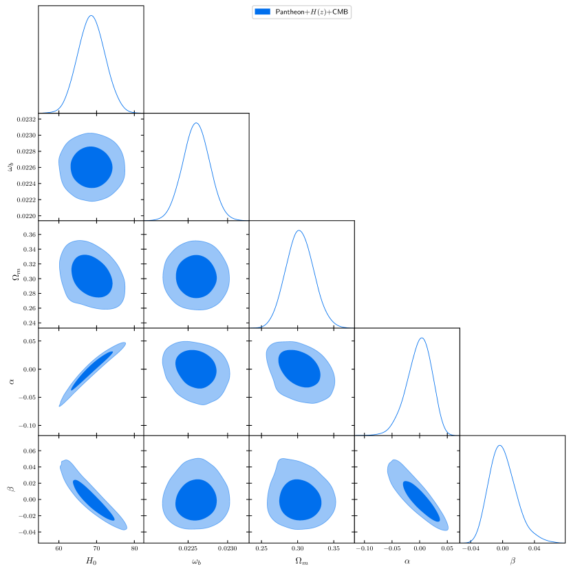
As can be seen on Fig. 9, there are strong correlations between the parameters and . One can also see that and are strongly constrained by this analysis. More details can be seen on Tab. 9.
| Parameter | () | () | |
|---|---|---|---|
| (km/s/Mpc) | |||
| 0 | |||
| 0 |
As can be seen on Tab. 9, the parameters and , which dictate the time dependence, are strongly constrained by CMB, leaving only small windows for variation. In fact, we may see that and at 95% c.l. This result has to be read with care, as we did not make a full CMB power spectrum analysis in the context of CDM. We have used, instead, distance priors which depend on models where the DM and DE are separately conserved. With that said, the results for the other parameters are similar to the ones obtained from Planck Planck2020 in the context of CDM, where it was found that km/s/Mpc, and . This is expected, as the values obtained for and are compatible with the CDM model.
In Tab. 9 we show, for completeness, the results for the subclasses of models which include a bare cosmological constant term, and . As it can be seen, the parameters are in general more constrained in the subclasses than in the general model, which is expected, as they have less free parameters. Again, these results shall be taken with care, as we have used an approximated treatment of the CMB results, but we may conclude that the interaction terms are quite constrained in the context of this analysis.
V Conclusion
We have analyzed 3 classes of CDM models against observations of SNe Ia, cosmic chronometers, and priors over the Hubble constant from Planck and SH0ES. We may conclude that 1 class of models, namely, , may be discarded by this analysis, mainly in the case of the Planck prior. In the case of the SH0ES prior, there is weak evidence against this. Models and can not be distinguished by this analysis.
At this point, it is important to mention that is the only considered model that does not have the standard CDM model as a particular case, once that . It seems that the data disfavor CDM models with this feature, at least for the classes of models analyzed here.
However, as one may see in Tables 2-7 and Figs. 4 and 8, the current analysis does not discard the possibility of an interaction between pressureless matter and vacuum. We also have seen in the current analysis, that the decaying of pressureless matter into a vacuum is in general favoured against vacuum decay, at least for the recent evolution of the Universe. The model is the only one where this situation changes in the past, allowing for a decay of the vacuum into pressureless matter.
This would indicate an obstacle for the classes of CDM models analysed here in order to alleviate the cosmological constant problem. On the other hand, a decaying of matter into vacuum may explain why only recently the vacuum density has become non-negligible.
As a final analysis, in the case of the more general model, , it was necessary to combine SNe Ia+ with CMB in order to constrain its free parameters. In this case, the time-dependence was quite constrained, but, as we have used an approximate method, a full analysis with the CMB power spectrum is needed in order to give the final verdict about this model.
We emphasize that in the present article, we have assumed the EoS of vacuum to be exactly . However, a recent result for the RVM is that the EoS of vacuum evolves with the cosmic history Pulido2022b . This would change our results and may be considered in future works.
Further analysis, considering other observational data, such as BAO, growth factor and full CMB power spectrum, in the lines of Peracaula2023 , for instance, in order to better constrain these models should be done in a forthcoming issue.
Acknowledgements.
SHP acknowledges financial support from Conselho Nacional de Desenvolvimento Científico e Tecnológico (CNPq) (No. 303583/2018-5 and 400924/2016-1). This study was financed in part by the Coordenação de Aperfeiçoamento de Pessoal de Nível Superior - Brasil (CAPES) - Finance Code 001.References
- (1) L. Perivolaropoulos and F. Skara, New Astron. Rev. 95 (2022), 101659 [arXiv:2105.05208 [astro-ph.CO]].
- (2) A. M. Öztaş, Mon. Not. Roy. Astron. Soc. 481 (2018) no.2, 2228-2234
- (3) R. G. Vishwakarma, Class. Quant. Grav. 18 (2001), 1159-1172 [arXiv:astro-ph/0012492 [astro-ph]].
- (4) J. M. Overduin and F. I. Cooperstock, Phys. Rev. D 58 (1998), 043506 [arXiv:astro-ph/9805260 [astro-ph]].
- (5) H. Azri and A. Bounames, Int. J. Mod. Phys. D 26 (2017) no.7, 1750060 [arXiv:1412.7567 [gr-qc]].
- (6) H. Azri and A. Bounames, Gen. Rel. Grav. 44 (2012), 2547-2561 [arXiv:1007.1948 [gr-qc]].
- (7) M. Szydłowski, Phys. Rev. D 91 (2015) no.12, 123538 [arXiv:1502.04737 [astro-ph.CO]].
- (8) M. Bruni, R. Maier and D. Wands, Phys. Rev. D 105 (2022) no.6, 063532 [arXiv:2111.01765 [gr-qc]].
- (9) G. Papagiannopoulos, P. Tsiapi, S. Basilakos and A. Paliathanasis, Eur. Phys. J. C 80 (2020) no.1, 55 [arXiv:1911.12431 [gr-qc]].
- (10) M. Benetti, W. Miranda, H. A. Borges, C. Pigozzo, S. Carneiro and J. S. Alcaniz, JCAP 12 (2019), 023 [arXiv:1908.07213 [astro-ph.CO]].
- (11) M. Benetti, H. Borges, C. Pigozzo, S. Carneiro and J. Alcaniz, JCAP 08 (2021), 014 [arXiv:2102.10123 [astro-ph.CO]].
- (12) I. L. Shapiro and J. Solà, Phys. Lett. B 475 (2000), 236-246 [arXiv:hep-ph/9910462 [hep-ph]].
- (13) I. L. Shapiro and J. Solà, JHEP 02 (2002), 006 [arXiv:hep-th/0012227 [hep-th]].
- (14) I. L. Shapiro, J. Solà, C. Espana-Bonet and P. Ruiz-Lapuente, Phys. Lett. B 574 (2003), 149-155 [arXiv:astro-ph/0303306 [astro-ph]].
- (15) A. Babic, B. Guberina, R. Horvat and H. Stefancic, Phys. Rev. D 65 (2002), 085002 [arXiv:hep-ph/0111207 [hep-ph]].
- (16) J. Solà, J. Phys. Conf. Ser. 453 (2013), 012015 [arXiv:1306.1527 [gr-qc]].
- (17) C. Moreno-Pulido and J. Solà, Eur. Phys. J. C 80 (2020) no.8, 692 [arXiv:2005.03164 [gr-qc]].
- (18) C. Moreno-Pulido and J. Solà Peracaula, Eur. Phys. J. C 82 (2022) no.6, 551 [arXiv:2201.05827 [gr-qc]].
- (19) C. Moreno-Pulido and J. Solà Peracaula, Eur. Phys. J. C 82 (2022) no.12, 1137 [arXiv:2207.07111 [gr-qc]].
- (20) C. Moreno-Pulido, J. Solà Peracaula and S. Cheraghchi, Eur. Phys. J. C 83 (2023) no.7, 637 [arXiv:2301.05205 [gr-qc]].
- (21) J. Solà Peracaula, Phil. Trans. Roy. Soc. Lond. A 380 (2022), 20210182 [arXiv:2203.13757 [gr-qc]].
- (22) J. Solà Peracaula, J. de Cruz Pérez and A. Gomez-Valent, Mon. Not. Roy. Astron. Soc. 478 (2018) no.4, 4357-4373 [arXiv:1703.08218 [astro-ph.CO]].
- (23) J. Solà Peracaula, A. Gomez-Valent, J. de Cruz Perez and C. Moreno-Pulido, Universe 9 (2023) no.6, 262 [arXiv:2304.11157 [astro-ph.CO]].
- (24) J. Solà Peracaula, A. Gómez-Valent, J. de Cruz Perez and C. Moreno-Pulido, EPL 134 (2021) no.1, 19001 [arXiv:2102.12758 [astro-ph.CO]].
- (25) J. Solà Peracaula, J. de Cruz Pérez and A. Gómez-Valent, EPL 121 (2018) no.3, 39001 [arXiv:1606.00450 [gr-qc]].
- (26) P. Tsiapi and S. Basilakos, Mon. Not. Roy. Astron. Soc. 485 (2019) no.2, 2505-2510 [arXiv:1810.12902 [astro-ph.CO]].
- (27) N. E. Mavromatos and J. Solà Peracaula, Eur. Phys. J. ST 230 (2021) no.9, 2077-2110 [arXiv:2012.07971 [hep-ph]].
- (28) J. Solà, A. Gómez-Valent and J. de Cruz Pérez, Astrophys. J. 836 (2017) no.1, 43 [arXiv:1602.02103 [astro-ph.CO]].
- (29) J. L. Lopez and D. V. Nanopoulos, Mod. Phys. Lett. A 11 (1996), 1-7 [arXiv:hep-ph/9501293 [hep-ph]].
- (30) W. Chen and Y. S. Wu, Phys. Rev. D 41 (1990), 695-698 [erratum: Phys. Rev. D 45 (1992), 4728]
- (31) M. Ozer and M. O. Taha, Phys. Lett. B 171 (1986), 363-365
- (32) M. Ozer and M. O. Taha, Nucl. Phys. B 287 (1987), 776-796
- (33) J. C. Carvalho, J. A. S. Lima and I. Waga, Phys. Rev. D 46 (1992), 2404-2407
- (34) J. A. S. Lima, E. L. D. Perico and G. J. M. Zilioti, Int. J. Mod. Phys. D 24 (2015) no.04, 1541006 [arXiv:1502.01913 [gr-qc]].
- (35) D. M. Scolnic et al. [Pan-STARRS1], Astrophys. J. 859 (2018) no.2, 101 [arXiv:1710.00845 [astro-ph.CO]].
- (36) M. Moresco, L. Amati, L. Amendola, S. Birrer, J. P. Blakeslee, M. Cantiello, A. Cimatti, J. Darling, M. Della Valle and M. Fishbach, et al. Living Rev. Rel. 25 (2022) no.1, 6 [arXiv:2201.07241 [astro-ph.CO]].
- (37) R. Sawada and Y. Suwa, Astrophys. J. 908 (2021) no.1, 6 [arXiv:2010.05615 [astro-ph.HE]].
- (38) N. Aghanim et al. [Planck], Astron. Astrophys. 641 (2020), A8 [arXiv:1807.06210 [astro-ph.CO]].
- (39) E. Di Valentino, O. Mena, S. Pan, L. Visinelli, W. Yang, A. Melchiorri, D. F. Mota, A. G. Riess and J. Silk, Class. Quant. Grav. 38 (2021) no.15, 153001 [arXiv:2103.01183 [astro-ph.CO]].
- (40) G. Schwarz, Annals Statist. 6 (1978), 461-464
- (41) A. R. Liddle, Mon. Not. Roy. Astron. Soc. 351 (2004), L49-L53 [arXiv:astro-ph/0401198 [astro-ph]].
- (42) J. F. Jesus, R. Valentim and F. Andrade-Oliveira, JCAP 09 (2017), 030 [arXiv:1612.04077 [astro-ph.CO]].
- (43) L. Chen, Q. G. Huang and K. Wang, JCAP 02 (2019), 028 [arXiv:1808.05724 [astro-ph.CO]].