Spin-Hall Current and Nonlocal Transport in Ferromagnet-Free Multi-band models for ${\rm SrTiO}_{3}$-Based Nanodevices in the presence of impurities

Abstract

We compute the spin-Hall conductance in a multiband model describing the two-dimensional electron gas formed at a LaAlO₃/SrTiO₃ interface in the presence of a finite concentration of impurities. Combining linear response theory with a systematic calculation of the impurity contributions to the self-energy, as well as to the vertex corrections of the relevant diagrams, we recover the full spin-Hall vs. sheet conductance dependence of LaAlO₃/SrTiO₃ as reported in Trier et al. [Nano Lett. 20, 395 (2020)], finding a very good agreement with the experimental data below and above the Lifshitz transition. In particular, we demonstrate that the multiband electronic structure leads to only a partial, instead of a complete, screening of the spin-Hall conductance, which decreases with increasing the carrier density. Our method can be generalized to other two-dimensional systems characterized by a broken inversion symmetry and multiband physics.

I Introduction

Recently, spintronics, a branch of electronics based on the manipulation of electron spin, rather than the charge, is emerging as a promising technology for information storing and processing, and for sensing Wolf et al. (2001); Vaz et al. (2019); Hirohata et al. (2020). Spin-injection in spintronic devices can be done by using ferromagnetic leads, however the efficiency of this process is usually low Chauleau et al. (2016); Song et al. (2017); Telesio et al. (2018). An alternative approach is to use semiconducting materials characterized by large charge to spin conversion efficiency. Here, a charge current can be converted into a spin current due to the Edelstein Edelstein (1990) and/or the spin-Hall (SH) effects Dyakonov and Perel (1971); Sinova et al. (2015). This is a particularly efficient process, for example, in some two-dimensional systems Qian et al. (2014); Nie et al. (2015); Safeer et al. (2019); Benítez et al. (2020); Safeer et al. (2020), and topological insulators (see, for instance, Ref. Farzaneh and Rakheja (2020) and references therein), characterized by breaking of the inversion symmetry due to a Rashba-type spin orbit interaction (SOI), even in the absence of ferromagnetic leads Trier et al. (2020).

The Edelstein effect consists of a spin-accumulation induced by an injected electrical current due to the presence of Rashba-split Fermi surfaces. The excess spin density diffuses across the system, thus giving rise to a net spin-polarized spin current perpendicular to the charge current, as the spin and the momentum of the carrier get “ locked”. At variance, the SH effect can either be extrinsic, i.e., related to the impurity scattering in the material, or intrinsic, due to the SOI related to the direct coupling (in the response function) between the electric and the spin currents Sinova et al. (2004).

An ideal platform to realize a versatile and tunable Rashba SOI in realistic devices is provided by the two-dimensional electron gas (2DEG) that emerges at the surface of SrTiO₃ (STO) and at the interface between STO and large gap band insulating oxides, like LaAlO₃ (LAO)King et al. (2014); Ohtomo and Hwang (2004); Chen et al. (2011); Rödel et al. (2016). Among other remarkable properties, the 2DEG possesses a strong tunability of the carrier density by gate voltages, which allows for a tuning of a Rashba-type SOI by electric field effect Caviglia et al. (2008, 2010); Trama et al. (2021); Lesne et al. (2016).

SrTiO₃-based nanodevices are very promising for spintronics, as they are characterized by one of the largest spin-charge conversion efficiencies among all materials, as shown in Refs. Varignon et al. (2018); Vaz et al. (2019). In Fig. 1 we sketch the experimental setup of Ref. Trier et al. (2020). Here, the charge current $I_{\rm c,in}$ injected (along the $y$ axis of the figure) at contacts 1 and 2 generates a net spin-current $I_{\rm s}$ diffusing in the bridge along the $x$ axis. A second spin-charge conversion at nearby contacts (3 and 4) turns $I_{\rm s}$ back into the charge current $I_{\rm c,out}$, thus giving rise to a nonlocal voltage drop and to a nonlocal resistance $R_{\rm NL}$.

$R_{\rm NL}$ is related to the spin diffusion length and to the spin-Hall angle $\gamma$ (note that $R_{\rm NL}$ is expected to be $\propto\gamma^{2}$   Abanin et al. (2009)), which, through a fitting, directly allows a measurements of the efficiency of the charge-to-spin conversion. In Ref. Trier et al. (2020) a spin-diffusion length up to 900 nm was estimated in the LAO/STO 2DEG. Moreover, a strong, non-monotonic, dependence of $\gamma$ as a function of the gate voltage $V_{g}$ was reported.

The spin-polarization direction, determined by measuring $R_{\rm NL}$ as a function of the magnetic field intensity and direction, is mainly along the out-of-plane $z$ direction (Fig. 1), consistent with the SH effect as the main mechanism. The resulting spin-Hall vs. longitudinal conductance was then compared to calculations assuming a multiband tight-binding model in the absence of disorder. While the overall non-monotonic dependence is captured by a clean multiband mode Trier et al. (2020), discrepancies can be noticed at low values of the chemical potential and at the Lifshitz transition, calling for further studies, in particular considering the role of realistic impurity scattering induced by nonmagnetic disorder.

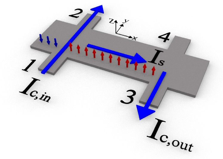
Figure 1: Sketch of the experimental setup of Trier et al. (2020). The charge current $I_{\rm c,in}$ injected at contacts 1 and 2 generates a net spin-current $I_{\rm s}$ diffusing in the bridge along the $x$-axis, which by a second spin-charge conversion at contacts 3 and 4 turns again into the charge current $I_{\rm c,out}$,

In this paper we develop a general approach to the spin-Hall conductance (SHC) in a multiband model with a SOI in the form characteristic of the 2DEG at a LAO/STO interface. In particular, we employ linear response theory (LRT) to compute the SHC by accounting for elastic scattering effects of nonmagnetic impurities in the 2DEG (which seems appropriate at low density of carriers Trier et al. (2020)). In addition, we compute the sheet conductance and the SHC in the multiband system with the band structure and the various parameters as in Ref. Trier et al. (2020).

Along our derivation, we systematically take into account the complex pattern of SOI in LAO/STO, both of atomic nature, as well as Rashba-type, due to the combined effect of the splitting of the Ti-$3d$ bands (which support the conduction in the 2DEG), determined by the lateral confinement Vaz et al. (2019), and to the inversion-symmetry breaking.

Throughout our analysis of the SH effect we show that, while any finite concentration of elastic impurity scatterers would fully screen to zero the SHC in a single-band Rashba 2DEG Mishchenko et al. (2004); Inoue et al. (2004); Khaetskii (2006); Raimondi and Schwab (2005); Dimitrova (2005), the multiband structure of the model, combined with the intraband and the inter-band SOI, leads to only a partial screening of the SHC, which shows a non-monotonic carrier density dependence consistent with the experimental results of Ref. Trier et al. (2020).

Our results for the sheet conductance show an excellent agreement with the experimental data, both from the qualitative, as well as from the quantitative point of view. When low-lying bands only are involved, our results for the SHC exhibit again an excellent quantitative (and qualitative) agreement with the experimental data. The model captures also the presence of a peak in the SHC when higher-energy bands come into play through the Lifshitz transition in the 2DEG, however, in this region the agreement is apparently less good, which calls for a deeper discussion of how the SHC should behave across the Lifshitz transition. Eventually, the agreement is recovered at a good level for larger values of $V_{g}$.

Our method allows us to derive in detail the impurity-induced vertex corrections to the SHC in a multiband system such as the 2DEG at the LAO/STO: it is a substantial extension of single-band models available to calculate the SHC in two dimensional systems, and can be easily generalized to any multi-band system. Here we focus on the “eight-band” model to recover the results of Ref. Trier et al. (2020), but we show how it can be generalized to other systems, such as a Rashba, single-band 2DEG, which we discuss in the Appendixes of our paper, or the “six-band” model, a simplified version of the eight-band one discussed, for instance, in Ref. Perroni et al. (2019).

In presenting our method and its applications, we organize our paper as follows:

• In Sec. II we present our method and how to apply it to a generic multiband, tight-binding model in the presence of a finite density of impurities.

• In Sec. III we introduce and discuss in detail the 8-band Hamiltonian describing the LAO/STO interface.

• In Sec. IV we compute the sheet and the spin-Hall conductance of the 8-band model in the presence of a finite density of impurities. Eventually, we discuss our results in relation to the experimental data of Ref. Trier et al. (2020).

• In Sec. V we provide our conclusions and present some possible further developments of our work.

  In the various appendices we provide several technical details of our derivation. In particular:

• In Appendix A we review the Kubo formulas for the response functions that we use to describe charge and/or spin transport.

• In Appendix B we present our approach to describing the effects of a finite density of impurity scattering centers on the various response functions.

• In Appendix C we review the paradigmatic calculation of the spin-Hall conductance in a lattice model for the two-dimensional Rashba Hamiltonian.

• In Appendix D we derive the effective, low-energy description of the 8-band model Hamiltonian in terms of a two-subband Rashba-like Hamiltonian.

• Finally, in the last appendix E we provide the mathematical details of our analytical derivation of the sheet conductance and of the spin-Hall conductance in the 8-band model.

II Multi-band model Hamiltonian with spin-orbit interaction

In this paper we add the impurity Hamiltonian on top of a specific model Hamiltonian describing a multiband system in the presence of atomic spin-orbit coupling Bistritzer et al. (2011), as well as inter-band inversion-symmetry breaking terms, providing an emergent Rashba interaction Caviglia et al. (2010); Michaeli et al. (2012). Given the grouping of the energy bands into quasi-degenerate doublets Khalsa et al. (2013), the SOI generically has matrix elements both intradoublet (the same), as well as interdoublets (different) Shanavas et al. (2014). Assuming lattice translational invariance, we employ a lattice Hamiltonian of the form

$$H=\sum_{\vec{k}}\>\sum_{\sigma,\sigma^{\prime}}c_{\vec{k},\sigma}^{\dagger}{\cal H}_{\sigma,\sigma^{\prime}}(\vec{k})c_{\vec{k},\sigma^{\prime}}\>\>\>\>,$$ (1)

with $\vec{k}$ being a generic point in the Brillouin zone and $\sigma$ being the “bare” band index (not to be confused with the spin index, with which it can nevertheless coincide in some cases, such as the single-band two-dimensional Rashba Hamiltonian). The (“undressed”) single-fermion operators in Eq.(1) obey the canonical anticommutation relations $\{c_{\vec{k},\sigma},c_{\vec{k}^{\prime},\sigma^{\prime}}^{\dagger}\}=\delta_{\vec{k},\vec{k}^{\prime}}\delta_{\sigma,\sigma^{\prime}}$. We also use $\Gamma_{\vec{k},\lambda}$ to denote the (“dressed”) eigenoperators of $H$, satisfying the anticommutation relations $\{\Gamma_{\vec{k},\lambda},\Gamma_{\vec{k}^{\prime},\lambda^{\prime}}\}=\delta_{\vec{k},\vec{k}^{\prime}}\delta_{\lambda,\lambda^{\prime}}$, as well as the canonical commutation relations

$$[\Gamma_{\vec{k},\lambda},H]=\epsilon_{\vec{k},\lambda}\Gamma_{\vec{k},\lambda}\>\>\>\>,$$ (2)

so that $\lambda$ is the “dressed band” label. The operators $\Gamma_{\vec{k},\lambda}$ and $c_{\vec{k},\sigma}$ are related to each other by an unitary transformation, according to

$$c_{\vec{k},\sigma}=\sum_{\lambda}w_{\sigma,\lambda}^{\vec{k}}\Gamma_{\vec{k},\lambda}\>\>\>\>,$$ (3)

with the transformation matrix elements satisfying the relations

$$\sum_{\lambda}w^{\vec{k}}_{\sigma,\lambda}[w^{\vec{k}}_{\sigma^{\prime},\lambda}]^{*}=\delta_{\sigma,\sigma^{\prime}}\;\;,$$

$$\sum_{\sigma}[w^{\vec{k}}_{\sigma,\lambda}]^{*}w^{\vec{k}}_{\sigma,\lambda^{\prime}}=\delta_{\lambda,\lambda^{\prime}}\>\>\>\>.$$ (4)

According to Eq. (3), it is possible to express any observable ${\cal O}$ that is bilinear in the undressed fermionic operators in the rotated basis, according to

$${\cal O} = \sum_{\vec{k},\vec{k}^{\prime}}\sum_{\sigma,\sigma^{\prime}}[{\cal O}]_{(\vec{k},\sigma);(\vec{k}^{\prime},\sigma^{\prime})}c_{\vec{k},\sigma}^{\dagger}c_{\vec{k}^{\prime},\sigma^{\prime}}$$ (5)

$$= \sum_{\vec{k},\vec{k}^{\prime}}\sum_{\lambda,\lambda^{\prime}}[{\cal O}]_{(\vec{k},\lambda);(\vec{k}^{\prime},\lambda^{\prime})}\Gamma_{\vec{k},\lambda}^{\dagger}\Gamma_{\vec{k}^{\prime},\lambda^{\prime}}\>\>\>\>,$$

with

$$[{\cal O}]_{(\vec{k},\lambda);(\vec{k}^{\prime},\lambda^{\prime})}=\sum_{\sigma,\sigma^{\prime}}[w_{\sigma,\lambda}^{\vec{k}}]^{*}w_{\sigma^{\prime},\lambda^{\prime}}^{\vec{k}^{\prime}}[{\cal O}]_{(\vec{k},\sigma);(\vec{k}^{\prime},\sigma^{\prime})}\>\>\>\>.$$ (6)

On top of the “clean” Hamiltonian in Eq. (1), we add disorder to our system by introducing an impurity scattering potential and a finite density of impurities. We do so by introducing, in real space, the white-noise impurity potential $V_{\rm Imp}(\vec{r})$ given by Borge et al. (2014)

$$V_{\rm Imp}(\vec{r})=\sum_{\vec{R}_{i}}U(\vec{r}-\vec{R}_{i})\;\;\;\;,$$ (7)

with $U(\vec{r})$ being the single-impurity scattering potential and the impurity scattering centers $\vec{R}_{j}$ randomly distributed over the system lattice. In Appendix B we perform a systematic derivation of the self-energy, as well as of the vertex corrections due to the finite density of impurities in our system.

In a single-band 2DEG with a Rashba-type SOI, it is well known that any finite amount of impurities provides a vertex correction that fully screens to zero the spin-Hall conductance Rashba (2004); Mishchenko et al. (2004); Inoue et al. (2004); Khaetskii (2006); Raimondi and Schwab (2005); Dimitrova (2005), while the general conditions at which the cancellation does, or does not, take place for impurity scattering with an arbitrary angular dependence, and for an arbitrary angular dependence of the spin-orbit field around the Fermi surface are discussed in Shytov et al. (2006) within the Boltzmann equation approach. Also, in Appendix C we apply our method to computing the SHC in a lattice model for a two-dimensional electron gas with Rashba SOI, finding a perfect, impurity induced, screening. At variance, as we show in the following in the multiband model describing the electronic states in ${\rm SrTiO}_{3}$-nanodevices Vivek et al. (2017); Perroni et al. (2019); Trier et al. (2020), the multiband structure itself determines a variable screening of the SHC. Moreover, the amount of screening, at a given density of impurities, depends on the position of the Fermi energy in the system and, therefore, it can be continuously tuned from being almost perfect to being negligible.

III The 8-band model Hamiltonian

We now focus onto the eight-band, tight-binding Hamiltonian describing the 2DEG that forms at a ${\rm LaAlO}_{3}$-${\rm SrTiO}_{3}$ (LAO/STO)-interface Huijben et al. (2017); Vaz et al. (2019); Trier et al. (2020). Basically, the perovskite structure of the background lattice induces an isotropic dispersion relation in the $t_{2g}$-bands of the Ti, which are responsible for the conduction in the 2DEG. In addition, the lateral confinement that determines the 2DEG splits the $d_{xy}$-subbands from the $d_{yz}$- and the $d_{zx}$-ones Vaz et al. (2019). A “minimal” (six-band) model accounting for such effects is based on retaining one band of each kind, for a total of six different subbands, taking into account the spin degree of freedom, as well Perroni et al. (2019). Following Ref. Trier et al. (2020), in this paper we include an additional pair of $d_{xy}$-subbands ($d_{xy;B}$), splitted above in energy with respect to the lower ($d_{xy;A}$) subbands with the same orbital character, but still below, with respect to the $d_{yz}$- and to the $d_{zx}$-subbands.

Defining the various labels as outlined above, we write the eight-band model Hamiltonian in the lattice momentum representation as

$$H_{\rm 8-band}=\sum_{\vec{k}}\>\sum_{\sigma,\sigma^{\prime}}c_{\vec{k},\sigma}^{\dagger}[{\cal H}_{\rm 8-band}(\vec{k})]_{\sigma,\sigma^{\prime}}c_{\vec{k},\sigma^{\prime}}\;\;\;\;,$$ (8)

with the sum over $\vec{k}$ taken over the full Brillouin zone, and $\sigma$ used to label single-particle operators $c_{\vec{k},\alpha,s}$, with $\alpha\in\{yz,zx,(xy;A),(xy;B)\}$ and $s\in\{\uparrow,\downarrow\}$. Using a block-notation with respect to the spin degree of freedom, we write the matrix ${\cal H}_{\rm 8-band}(\vec{k})$ in Eq.(8) as

$${\cal H}_{\rm 8-band}(\vec{k})={\cal H}_{0}(\vec{k})+{\cal H}_{\rm SO}+{\cal H}_{Z}({\vec{k}})\>\>\>\>,$$ (9)

with the various matrices at the right-hand side of Eq.(9) defined as it follows:

• The band dispersion relation:

  $${\cal H}_{0}(\vec{k})=\left[\begin{array}[]{cccc}\epsilon_{yz}(\vec{k}){\bf I}&{\bf 0}&{\bf 0}&{\bf 0}\\ {\bf 0}&\epsilon_{zx}(\vec{k}){\bf I}&{\bf 0}&{\bf 0}\\ {\bf 0}&{\bf 0}&\epsilon_{xy;A}(\vec{k}){\bf I}&{\bf 0}\\ {\bf 0}&{\bf 0}&{\bf 0}&\epsilon_{xy;B}(\vec{k}){\bf I}\end{array}\right]\>\>\>\>,$$ (10)

  with

  $${\bf 0}=\left[\begin{array}[]{cc}0&0\\ 0&0\end{array}\right]\;\;,\;{\bf I}=\left[\begin{array}[]{cc}1&0\\ 0&1\end{array}\right]\>\>\>\>,$$ (11)

  and

  $$\epsilon_{yz}(\vec{k}) = 2t_{2}[1-\cos(k_{x})]+2t_{1}[1-\cos(k_{y})]\;,$$

  $$\epsilon_{zx}(\vec{k}) = 2t_{1}[1-\cos(k_{x})]+2t_{2}[1-\cos(k_{y})]\;,$$

  $$\epsilon_{xy;(A,B)}(\vec{k}) = 2t_{1}[2-\cos(k_{x})-\cos(k_{y})]-\Delta_{(A,B)}\>\>\>\>.$$ (12)

• The atomic spin-orbit Hamiltonian:

  $${\cal H}_{\rm SO}=\lambda_{\rm SO}\>\left[\begin{array}[]{cccc}{\bf 0}&i{\bf\sigma}^{z}&-i{\bf\sigma}^{y}&-i{\bf\sigma}^{y}\\ -i{\bf\sigma}^{z}&{\bf 0}&i{\bf\sigma}^{x}&i{\bf\sigma}^{x}\\ i{\bf\sigma}^{y}&-i{\bf\sigma}^{x}&{\bf 0}&{\bf 0}\\ i{\bf\sigma}^{y}&-i{\bf\sigma}^{x}&{\bf 0}&{\bf 0}\end{array}\right]\;\;\;\;.$$ (13)

• The inter-band inversion-symmetry breaking interaction:

  $${\cal H}_{Z}(\vec{k})=\left[\begin{array}[]{cccc}{\bf 0}&{\bf 0}&-if_{1}^{X}(\vec{k}){\bf I}&-if_{2}^{X}(\vec{k}){\bf I}\\ {\bf 0}&{\bf 0}&-if_{1}^{Y}(\vec{k}){\bf I}&-if_{2}^{Y}(\vec{k}){\bf I}\\ if_{1}^{X}(\vec{k}){\bf I}&if_{1}^{Y}(\vec{k}){\bf I}&{\bf 0}&{\bf 0}\\ if_{2}^{X}(\vec{k}){\bf I}&if_{2}^{Y}(\vec{k}){\bf I}&{\bf 0}&{\bf 0}\end{array}\right]\;\;\;\;,$$ (14)

  with

  $$f_{1,2}^{X}(\vec{k}) = 2\gamma_{1,2}\sin(k_{x})\;,$$

  $$f_{1,2}^{Y}(\vec{k}) = 2\gamma_{1,2}\sin(k_{y})\>\>\>\>.$$ (15)

In addition to the various contributions at the right-hand side of Eq.(9), in a nonzero applied magnetic field, an additional spin-Zeeman interaction term $H_{M}$ term appears, $H_{M}=-\vec{M}\cdot\vec{S}$, with $\vec{M}$ being the Zeeman field and $\vec{S}$ being the total spin. As, throughout our derivation, we always set $\vec{M}=0$, we do not include $H_{M}$ in Eq.(9).

In doing our calculation, we took the numerical estimate of the various parameters as presented in Ref. Trier et al. (2020), which we summarize in Table 1.

Parameter	Numerical value (meV)
$t_{1}$	388
$t_{2}$	31
$\Delta_{A}$	150
$\Delta_{B}$	30
$\gamma_{1}$	20
$\gamma_{2}$	5
$\lambda_{\rm SO}$	8.3

Table 1: Numerical values of the parameters of the eight-band model (measured in meV) as from Trier et al. (2020).

In Figure 2 we plot the energy levels of the full Hamiltonian in Eq.(9) along high-symmetry lines of the Brillouin zone, by choosing the other system parameters as in table 1. The combined effect of the atomic SOI and of the inversion-symmetry breaking terms also splits each doublet, as evidenced in the figure, even at zero Zeeman field. The colored horizontal dashed lines correspond to the “opening” of the higher-energy doublets. As we discuss in the following, as long as the chemical potential is much below the opening of the green doublet (dashed horizontal green line – about 45 meV), the 2DEG behaves as a “standard” spinful, single-band Rashba 2DEG (see Appendix D for a detailed model calculation), although the multi-band structure of the system strongly affects the impurity-induced screening of the spin-Hall conductance.

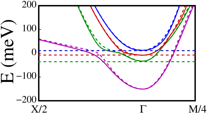
Figure 2: Energy levels of the full Hamiltonian in Eq.(9) computed by choosing the other system parameters as in Table 1. The colored, horizontal dashed lines mark the opening (on increasing the energy) of higher-energy doublets.

Above the green dashed line the second doublet becomes available: as we discuss in the following, for what concerns spin transport, the green doublet is pretty similar to the magenta one, as they both share a high overlap with, respectively, the $d_{xy;A}$ and the $d_{xy;B}$ subbands, very similar in their properties.

Moving across the dashed horizontal red line, higher-energy subbands start to be populated. As it may be readily checked by direct calculations, these subbands have a high overlap with the $d_{yz}$ and the $d_{zx}$ subbands, which have different symmetries, with respect to the lower-energy $d_{xy;A/B}$ subbands. At the onset of the higher-energy subbands, a Lifshitz transition (LT) is expected to take place Joshua et al. (2012), with a massive and sudden increase in the density of states due to the opening of the higher subbands, as evidenced in Appendix E. As we evidence in the following, the LT carries along remarkable changes in the (spin) transport properties of the system, with relevant consequences on the experimental results.

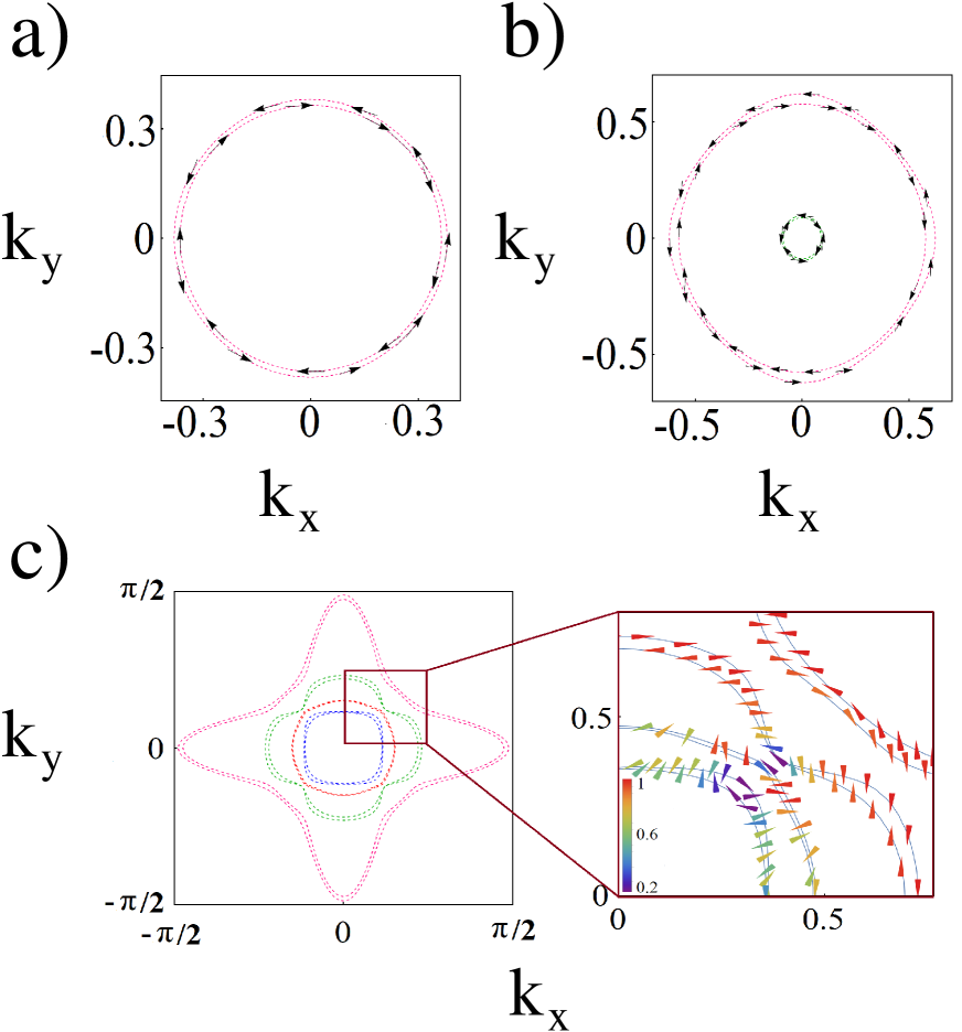
Figure 3: (a): Spin pattern within the $xy$-plane in spin space as a function of the momentum $\vec{k}$ computed using the eight-band model Hamiltonian in Eq. (9) with $\vec{M}=0$ and at energy $E=-100$ meV. (b): Same as in (a), but with $E=-30$ meV. (c): Same as in (a) and (b), but with $E=+55$ meV. The spin pattern is evidenced in the zoom in the right-hand subpanel. In all the cases the out-of-plane spin component is zero, due to the absence of an applied magnetic field.

Specifically, on increasing the chemical potential, we have computed, at fixed energy $E$, the spin pattern within the $xy$-plane in spin space as a function of the momentum $\vec{k}$ within the Brillouin zone. In Fig. 3 we report the results of our derivation at energy $E=-100$ meV, $E=-30$ meV, and $E=+55$ meV. In Fig. 3(a) we show our results at $E=-100$ meV. We clearly recognize the typical spin pattern of a Rashba 2DEG Sinova et al. (2004). As Fig. 3(a) evidences, the opposite spin orientation in the two subbands corresponds to an opposite value of the Rashba effective magnetic field acting over the electron spin and, accordingly, to opposite, over-all contributions to the total spin current generated by an applied electric field ${\cal E}^{y}$. In fact, that result is consistent with our derivation of Appendix D, where we show that, for $-\Delta_{A}<\mu<-\Delta_{B}$, with the band offsets $\Delta_{A,B}$ defined in the last one of Eqs. (12), the eight-band model is effectively described by the Rashba Hamiltonian $H_{xy}$ in Eq. (106). We therefore expect, in the absence of disorder, a quantized jump (by $e^{2}/h$) in the spin-Hall conductance $\sigma_{xy}^{z}$ at the onset of the first doublet and a featureless, constant value $\sigma_{xy}^{z}$ on further increasing $\mu$ (see Appendix C for details). As we discuss in the following, this is exactly what happens in the absence of disorder.

In Fig.3(b) we draw states at energy $E=-30$ meV. These belong to the first two pairs of subbands. As it appears from the figure, the sign of the Rashba SOI is the same in both pairs of subbands: this suggests that, at the onset of the second pair of subbands, an additional jump, similar to the one at the start of the first doublet, should appear, with a corresponding doubling in the quantized value of $\sigma_{xy}^{z}$.

A drastic change happens at $E=+55$ meV, when all four of the doublets are involved [see Fig. 3(c)]. Indeed, from the zoom of the highlighted region, we clearly see how the mixing with higher effective mass bands implies that different pairs of subbands show different signs in the net SOI (in fact, our result mimics the one of Ref. Johansson et al. (2021), despite the different values of the model parameters used in that paper). At the onset of the (mostly $yz$- and $zx$-like) higher-energy subbands, we therefore expect a breakdown of the monotonical increase of $\sigma_{xy}^{z}$ with $\mu$ and, due to the large difference in the effective mass between the lower and the upper doublets, even a possible change of sign in the spin-Hall conductance, at a certain value of $\mu$. As we will see in the following, this is, in fact, what happens when going through a full calculation of $\sigma_{xy}^{z}$ in the eight-band model, even after impurities are added to the system. In addition, while our sketch of the spin orientation in Fig. 3(a)- 3(c) is intended just to evidence the spin pattern at equal energy curves, close to the Lifshitz transition, it is important to consider the modulus of the average spin polarization, in particular close to the avoided crossing directions (in our case the diagonals of the Brillouin zone), due to its relation with alternative possible sources of a nonlocal resistance signal, such as the Edelstein effect Johansson et al. (2021). For this reason, in the zoom of Fig. 3(c), we provide the modulus of the average spin polarization in the color code specified in the figure itself, thus evidencing a reduction in the modulus of the average spin polarization over the avoided crossing directions similar to the one found in Ref. Johansson et al. (2021).

We now provide the results of our calculations of the sheet conductance, as well as of the spin-Hall conductance, in the eight-band model, in the clean limit, as well as in the presence of a finite impurity concentration.

IV The sheet conductance and the spin-Hall conductance in the 8-band model

To compute the sheet conductance of the 8-band model of section III, $\sigma_{s}$, we use the analytical expression of Appendix E, which we derive by means of a systematic implementation of the formalism of Appendixes A and B. In particular, having numerically checked that the vertex corrections in Eq.(112) provide a negligible contribution to $\sigma_{s}$, we perform our calculation by using Eq. (25) of Appendix A, with the single-particle Green’s functions including the finite, impurity-induced, imaginary part of the self-energy. Specifically, we set

$$\sigma_{s}=\frac{1}{V}\sum_{\vec{k}}\>\sum_{\lambda,\lambda^{{}^{\prime}}}[j_{{\rm ch},x}]_{(\vec{k},\lambda);(\vec{k},\lambda^{{}^{\prime}})}[j_{{\rm ch},x}]_{(\vec{k},\lambda^{{}^{\prime}});(\vec{k},\lambda)}$$

$$\times\int\frac{d\bar{\omega}}{2\pi}\>\Biggl{\{}g_{(\vec{k},\lambda)}^{<}(\bar{\omega})\partial_{\omega}g_{(\vec{k},\lambda^{{}^{\prime}})}^{R}(\bar{\omega})+g_{(\vec{k},\lambda)}^{A}(\bar{\omega})\partial_{\omega}g_{(\vec{k},\lambda^{{}^{\prime}})}^{<}(\bar{\omega})\Biggr{\}}\>,$$

(16)

with $V$ being the system volume, $[j_{{\rm ch},a}]_{(\vec{k},\lambda);(\vec{k},\lambda^{\prime})}$ being the charge current matrix elements in the basis of the single-particle eigenstates of ${\cal H}_{\rm 8-band}(\vec{k})$, and the single particle Green-Keldysh functions $g_{(\vec{k},\lambda)}^{A,R,<}(\omega)$ being defined in Appendix B.1. The impurity concentration determines, according to Eq.(46) of appendix B, a finite lifetime $\tau_{\rm Imp}^{\lambda}$ for the quasiparticle excitations in band $\lambda$, which enters the corresponding Green’s functions according to Eq.(45). Due to the relation between the impurity concentration and the finite quasiparticle lifetime, as we discuss in Appendix B, we take into account the former through the latter, by using for $\tau_{\rm Imp}^{\lambda}$ the $\lambda$-independent value $\tau_{\rm Imp}=3\>{\rm ps}$, as from the measures of Ref.Trier et al. (2020).

In Figure 4 we plot our result for $\sigma_{s}$ (in units of $e^{2}/h$) as a function of $\mu$, computed using Eq.(25) as discussed before (blue curve). For comparison, we also plot the experimental data corresponding to the measures of Ref. Trier et al. (2020) (black full squares). Apparently, there is a pretty good agreement between the two sets of data: in particular, both in the theoretical curve, as well as in the experimental data, we note the sudden change in the slope of $\sigma_{s}$ at the onset of the higher-energy bands, at $\mu$ slightly higher than 0, which evidences the sudden change in the density of state at the LT.

Close to the upper bound of the interval of values of $\mu$ that we consider ($\mu\in[-150\>{\rm meV},150\;{\rm meV}]$) the theoretical curve seems to become slightly higher than the last experimental point. This might be a signal of an (expected) breakdown of our approximation at large values of $\mu$. Yet, the agreement between the analytical and the experimental results is pretty good throughout almost all the interval of values covered by the experiment of Ref. Trier et al. (2020).

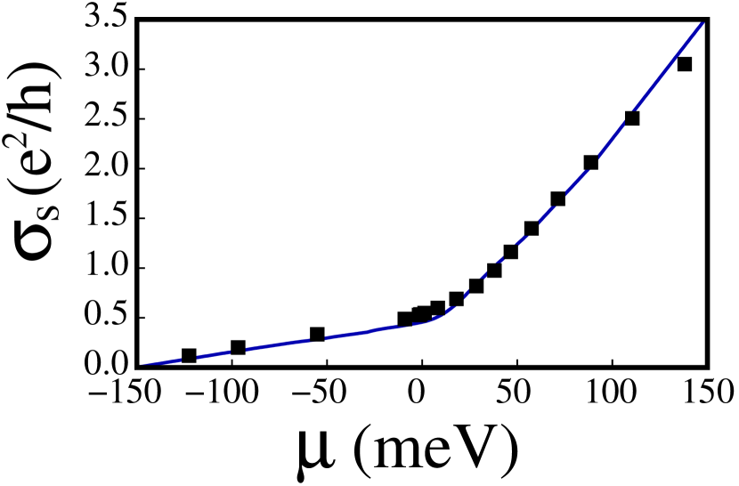
Figure 4: $\sigma_{s}$ as a function of $\mu$ (in units of $e^{2}/h$), computed according to Eq.(111) (blue curve); $\sigma_{s}$ experimentally measured, as reported in Ref. Trier et al. (2020) (black full squares). As discussed in the main text, we have accounted for the finite impurity concentration by setting the quasiparticle lifetime $\tau_{\rm Imp}=3\>{\rm ps}$, in agreement with the experimental results of Ref. Trier et al. (2020) .

We now consider the spin-Hall conductance $\sigma_{xy}^{z}$. Along the derivation of Appendix A and B, we find that the corresponding mathematical expression can be derived from Eq.(16) by substituting the first charge-current vertex, $[j_{{\rm ch},x}]_{(\vec{k},\lambda);(\vec{k},\lambda^{\prime})}$, with the fully dressed spin-current vertex $[j_{{\rm sp},x}^{z}]_{(\vec{k},\lambda);(\vec{k},\lambda^{\prime})}$ and the second one, $[j_{{\rm ch},x}]_{(\vec{k},\lambda^{\prime});(\vec{k},\lambda)}$, with $[j_{{\rm ch},y}]_{(\vec{k},\lambda^{\prime});(\vec{k},\lambda)}$. Within the approach of Appendix A, we perform our calculation using the formulas for $\sigma_{xy}^{z}$ for a homogeneous system. In fact, as it is typical for the spin-Hall effect, the spin current is established over typical length scales of the order of the electron mean free path Abanin et al. (2009), which we assume to be much smaller than the width of the sample we consider, as well as of the distance between the contacts Trier et al. (2020). Eventually, this enables us not to consider possible inhomogeneities in the spin current in the sample due to finite-size effects and allows us to resort to the formulas we employ in Appendix A.

For the sake of the discussion and also to interpret the results in terms of an effective Rashba-type SOI, we begin by computing $\sigma_{xy}^{z}$ as a function of $\mu$ in the “clean limit”, that is, without adding impurities to the sample. To do so, we use Eq.(113) of Appendix E, by replacing $g_{(\vec{k},\lambda)}^{R/A}(\omega)$ with their counterparts in the clean limit, $g_{(\vec{k},\lambda)}^{R/A;(0)}(\omega)$ in Eq.(39)

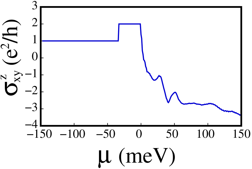
Figure 5: Spin-Hall conductance $\sigma_{xy}^{z}$ computed in the eight-band model using the full Hamiltonian in Eq.(9), by neglecting the effects of the impurities (“the clean limit”), as a function of the chemical potential $\mu$ for $-150{\rm meV}\leq\mu\leq 150{\rm meV}$. The quantized first two plateaus ($\mu\leq 0$) evidence the two-dimensional Rashba-type nature of the effective spin-orbit interaction in the first two energy doublets of Fig. 2.

In Fig. 5 we show the results of our calculation. We note that, as soon as $\mu$ “hits” the bottom of the first $d_{xy;A}$-like subband, $\sigma_{xy}^{z}$ suddenly jumps from 0 to $e^{2}/h$. A similar sudden, quantized jump takes place as $\mu$ crosses the bottom of the second doublet of energy eigenstates. As we review in detail in Appendix C, this is the typical behavior of the SHC in a lattice model of a Rashba 2DEG, which is consistent with the effective description of the eight-band model in terms of two, coupled Rashba-type Hamiltonians, at energies below the onset of the $yz$- and of the $zx$-like subbands (see Appendix D for details).

Moving toward higher value of $\mu$, we see that the regular behavior of $\sigma_{xy}^{z}$, made out of sharp jumps between quantized plateaus, suddenly changes when the higher-energy doublets set in. In fact, this comes along a drastical change in the effective Rashba SOI within each doublet. From Fig. 3 we see that, while the first two doublets both host an effective Rashba SOI with coupling strengths of the same sign (which is consistent with the two plateaus in the left part of the plot in Fig. 5), as soon as the $yz$- and the $zx$-like subbands get involved, the sign of the Rashba SOI from different doublets of subbands can be different and, more importantly, the sign of the Rashba coupling strength in subbands with higher effective mass is opposite to the one of the $d_{xy;A}$-like doublet. Thus, two different effects are expected to arise at the onset of the higher subbands: a strong increase in $\sigma_{xy}^{z}$, due to the larger carrier density, accompanied by a sudden change in the sign of the SHC itself, for the reason discussed above and evidenced in Fig. 3. Apparently, this is exactly the feature that shows up in Fig. 5 for $\mu$ slightly greater than 0, the following oscillations being likely due to the sequential changes in sign of the effective Rashba SOI in the intermediate-energy doublets, as $\mu$ gets larger Trier et al. (2020). We now discuss how Fig. 5 is modified by adding impurities to the system.

The behavior of the SHC in the presence of a finite density of impurities is strictly related to the mechanism behind the nonlocal resistance in SrTiO₃-based devices. In Ref. Trier et al. (2020) a systematic analysis of all the possible different mechanisms that could potentially lead to a nonlocal resistance in the system has been gone through, similar to what has been done in Refs. Nachawaty et al. (2018); Tagliacozzo et al. (2019) for graphene close to the charge-neutrality point. Having ruled out all the possible alternatives, the only left over reasonable explanations rely on either the Edelstein effect Edelstein (1990), or over the spin-Hall effect Sinova et al. (2004) (or a combination of the two of them). Nevertheless, the direct measurement of the spin polarization via the Hanle precession revealed that the electron spins are mostly polarized orthogonal to the electronic 2DEG, which rules out the Edelstein effect, as well, leaving SH effect as the only possible mechanism responsible for the measured nonlocal resistance Trier et al. (2020).

In the two-band Rashba model the presence of a finite impurity concentration is known to fully cancel the SHC by “compensating” the terms $\sigma_{xy;A}^{z}$, computed as in Eq. (113), with the vertex correction $\sigma_{xy;B}^{z}$, in Eq. (115) Mishchenko et al. (2004); Inoue et al. (2004); Khaetskii (2006); Raimondi and Schwab (2005); Dimitrova (2005) (see also Appendix C for details). At variance, as we are going to show by direct calculation, due to the complex inter-band mixing, the SHC in the eight-band model is affected only partially by the presence of disorder: the cancellation strongly depends on $\mu$ and, more importantly, it is never complete. This leaves room for a finite SHC in the eight-band model, even in the presence of a finite density of impurities in the system, which is apparently consistent with the experimental results of Ref. Trier et al. (2020).

To spell out in detail the role of the two contributions to $\sigma_{xy}^{z}$, we now separately discuss the two of them. In Fig.6, we plot our results for $\sigma_{xy;A}^{z}$ as a function of $\mu$ for $-150\>{\rm meV}\leq\mu\leq 150\>{\rm meV}$, computed according to Eq. (113) by using the parameters in Table 1 and by setting $\tau_{\rm e}=3$ ps. Remarkably, we can already see how adding the finite quasiparticle lifetime already strongly alters the behavior of $\sigma_{xy}^{z}$, compared to the clean limit of Fig.5. Yet, differently from what happens for the sheet conductance, we now show how, in this case, the vertex corrections have an important weight in the final result.

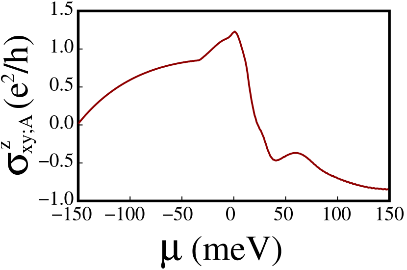
Figure 6: Spin-Hall conductance $\sigma_{xy;A}^{z}$ (without vertex corrections) computed, as a function of $\mu$, within the eight-band model, by using the parameters in Table 1 and by setting $\tau_{\rm e}=3$ ps in the dressed single-particle Green’s functions.

To compute $\sigma_{xy;B}^{z}$, we use Eq.(115) of Appendix E. In Fig.7 we plot the corresponding result for the “full” spin-Hall conductance $\sigma_{xy}^{z}=\sigma_{xy;A}^{z}+\sigma_{xy;B}^{z}$, including the effects of the vertex corrections. Looking at the plot, we note that there is a large window of values of $\mu$, from $\mu=-150$ meV to the onset of the high-energy subbands, where the vertex correction screens $\sigma_{xy}^{z}$ to a “quasilinear” dependence on $\mu$ at its onset. A minor, though clearly visible, change in the slope takes place at the onset of the second doublet: the change in the slope is the remnant, after the screening, of the second jump between the quantized values of $\sigma_{xy}^{z}$ in Fig.5. A relatively sharp decrease in the spin-Hall conductance takes place as soon as $\mu$ crosses the bottom of the two high-energy subbands. For $\mu$ slightly larger than 0, $\sigma_{xy}^{z}$ first increases and eventually crosses 0 and becomes negative. This is strictly connected with the onset of the higher-energy doublets which, as we highlighted before, provide contributions to $\sigma_{xy}^{z}$ opposite in sign with respect to the ones arising from the lower doublet. Higher-energy doublets are indeed characterized by an effective Rashba SOI of opposite sign, with respect to the lower-energy ones, and by a much higher density of states (at the band onset).

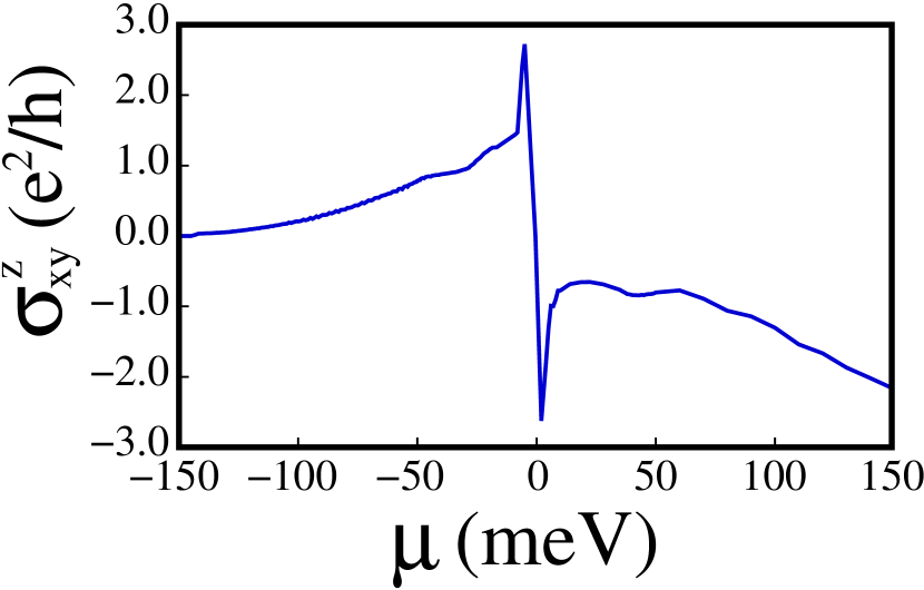
Figure 7: Spin-Hall conductance $\sigma_{xy}^{z}=\sigma_{xy;A}^{z}+\sigma_{xy;B}^{z}$(including vertex corrections) computed, as a function of $\mu$, within the eight-band model, by using the parameters in Table 1 and by setting $\tau_{\rm e}=3$ ps in the dressed single-particle Green’s functions.

We now discuss our results in comparison with the experimental data of Ref. Trier et al. (2020). To do so, we mimic the presentation of that paper by combining the results of Figs. 4 and 7 to display our results for $|\sigma_{xy}^{z}|$ as a function of our theoretically computed sheet conductance $\sigma_{s}$ (note that we consider the absolute value of $|\sigma_{xy}^{z}|$ to make a rigorous comparison with the experimental results of Ref. Trier et al. (2020), where they measure the spin-Hall conductance from the square root of the squared spin-Hall angle, which appears in the formula for the nonlocal resistance, [Eq.(1) of the paper. To evidence the importance of accounting for impurity-induced vertex corrections, in Fig. 8 we synoptically show the corresponding plots of both $|\sigma_{xy}^{z}|$ (computed by taking the absolute of $\sigma_{xy;A}^{z}+\sigma_{xy;B}^{z}$ – blue curve) and of $|\sigma_{xy;A}^{z}|$ (red curve), together with the experimental points corresponding to Fig. 4(c) of Ref. Trier et al. (2020) (black full squares).

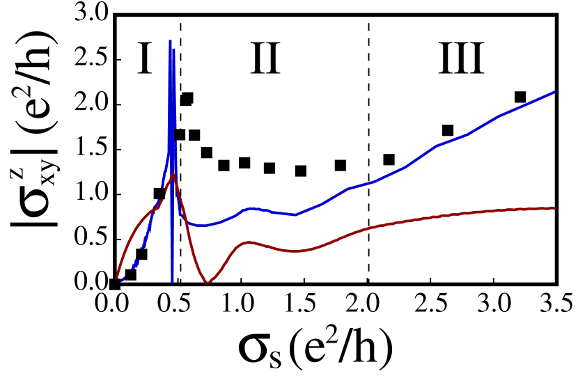
Figure 8: Solid blue line: (absolute value of the) spin-Hall conductance $|\sigma_{xy}^{z}|$ as in Fig. 7 drawn as a function of the sheet conductance $\sigma_{s}$ in Fig. 4; Solid red line: (absolute value of the) spin-Hall conductance without vertex corrections, $|\sigma_{xy;A}^{z}|$, as in Fig.6 drawn as a function of the sheet conductance $\sigma_{s}$ in Fig.4; Black full squares: experimental results for $\sigma_{xy}^{z}$ as a function of $\sigma_{s}$ as presented in Ref. Trier et al. (2020). The dashed vertical lines mark the splitting of the graph into the regions I,II and III, as discussed in the text.

In analyzing Fig.8 we split the graph into three regions: region I, for $0\leq\sigma_{s}\leq e^{2}/(2h)$, region II, for $e^{2}/(2h)\leq\sigma_{s}\leq 2e^{2}/h$, region III, for $2e^{2}/h\leq\sigma_{s}$.

Region I roughly corresponds to the part of the diagram before the onset of the high-energy, $yz$-like and $zx$-like, subbands in which, as it emerges from our analysis of Appendix D and from Fig.3, the two active $xy$-like subbands exhibit an effective Rashba SOI of the same sign in both bands. A synoptical numerical analysis of the data shown in Figs.4,8,11 also evidences how region I corresponds to the interval of values of $\mu$ where only the lowest-energy doublets contributes the vertex corrections, $\sigma_{xy;B}^{z}$, which we reliably compute within our approach, that is expected to work well in the low-density region of the system, by using Eq. (110) of Appendix E. In fact, we see that there is a perfect collapse of the experimental data onto the analytical blue curve: on one hand this shows the reliability of our method in this region, on the other hand, it evidences the importance of pertinently accounting for the vertex corrections. Indeed, the corresponding (red) curve, derived without taking into account the term $\sigma_{xy;B}^{z}$, clearly does not fit the experimental points.

Leaving aside region II, for the time being, let us focus onto region III of Fig. 8. Region III is characterized by a much higher carrier density than region I. Moreover, as we readily infer from Fig. 11, there is also, in this region, a finite contribution to Eq. (108) from all the four doublets of subband although, just as in region I, there is a single doublet (the lowest-energy one) that takes over with respect to the other ones. This makes us employ the approximate method outlined in Appendix E to pertinently weight the four involved doublets. Yet, despite the possibly oversimplified approach we use here, from the plot of Fig. 8 we see again quite a good agreement between the experimental points and the analytical curve, with just a minor undershooting of the latter which could possibly be fixed by, for instance, refining our approach by going through a systematic fitting procedure of the normalization factor in front of the vertex correction. Importantly, by synoptically looking at the red and at the blue curve of Fig. 8 we see how also in region III, it is fundamental to add vertex corrections to the final expression for $\sigma_{xy}^{z}$, in order to recover a good agreement between experiment and theory. Apparently, our results imply that contributions to the spin-Hall conductance arising from vertex corrections are always relevant, although their precise numerical estimate deserves a more refined modulation than the one behind Eq. (110). In addition, as evidenced by Fig.S4 of the Supplemental Material of Ref. Trier et al. (2020), the contribution to $\tau_{\rm Imp}$ arising from inelastic scattering processes should be taken into account, as well. All these further extensions of our derivation, although being definitely relevant to improve the numerical match between theory and experiment, go beyond the scope of this work, where we focus on the role of impurities to catch the main features of the experiments of Ref. Trier et al. (2020). We will possibly consider them in further developments of our investigation. Yet, it is worth stressing once more the good agreement of our theoretical calculations with the experimental data, despite the possibly oversimplified model we are employing here.

We finally discuss region II. At a first glance, in this region the agreement between the experimental data of Ref. Trier et al. (2020) and our analytical results is not as good as in the other two regions. Indeed, first of all we note that the experimental data seem to exhibit a peak in $|\sigma_{xy}^{z}|$ for $\sigma_{s}^{*}\approx 0.6e^{2}/h$, while, as it is clearly evidenced in Figs. 6 and 7, our analytical results, instead, show a zero around that value of $\sigma_{s}$, whether the vertex corrections are included, or not. As we discuss above, due to the different sign of the effective SOI interaction arising within the various energy doublet, it is somehow expected that $\sigma_{xy}^{z}$ crosses zero at some finite value of $\sigma_{s}$, roughly corresponding to the onset of the higher-energy doublets. However, due to the rather small hybridization between those last subbands and the lower-lying ones, we also expect that the crossing takes place sharply, within a small interval of variation of $\mu$, as also apparently shown in Fig. 7. Once switching to $|\sigma_{xy}^{z}|$, as we do in drawing Fig. 8, the zero-crossing feature trades for a sharp double peak which, due to the limited number of experimental points in Ref. Trier et al. (2020) around $\sigma_{s}^{*}$, might very well be experimentally seen as a single peak. An additional observation concerns the apparent offset, present throughout all region II, between the experimental data and the analytical curve, which apparently underestimates $\sigma_{xy}^{z}$, particularly close to the left-hand endpoint of the region, although the agreement between the experiment and the theory becomes better on moving towards the right-hand end point of region II. While we discuss more about this point below, here we stress how the agreement could be in principle improved by a pertinent refining of our method for estimating the prefactor in front of the vertex corrections and that, more importantly, the main trend of the theoretical curve as a function of $\sigma_{s}$ is basically consistent with the experimental data throughout Region II, as well. In any case, at least from the conclusions one may recover from Fig.3 about the Rashba SOI in each doublet, a zero-crossing of $|\sigma_{xy}^{z}|$ should be expected, right after the onset of the higher-energy doublets. In addition to the previous arguments, we note a remarkable, experimentally measured, decrease and increase of the spin-Hall angle $\gamma$ (although not all the way down to 0), which is evidenced in Fig.3(c) of Ref. Trier et al. (2020), at the value of the gate voltage that corresponds to $\sigma_{s}^{*}$. In view of above arguments and given the good agreement in regions I and III between our results and the experimental data, a refinement of the $\sigma_{xy}^{z}$ measurements around $\sigma_{s}^{*}$ would be highly desirable.

On the theory side, one could improve the modeling of the system by introducing scattering from finite-range impurities. Indeed, the scattering potential could present a correlation length consistent with experiments on negative magnetoresistance driven by spin-orbit coupling and scattering by dislocations Diez et al. (2015). This could give a contribution in the region II, since the anisotropic scattering could suppress backscattering processes within the outer Fermi surface with large average Fermi momentum, while still allowing for interband scattering. This should be accompanied by a quasiparticle lifetime which can be smaller for the inner bands with smaller average Fermi momenta. The induced imbalance could enhance the values of spin-Hall conductance in the region II, while leaving the sheet conductance poorly affected.

A possible extension of our work could possibly involve carrying out the analysis of the spin-, as well as of the orbital-, Edelstein effect. Indeed, while in Ref. Trier et al. (2020) a contribution to the nonlocal resistivity from the Edelstein effect was ruled out from the dependence of the Hanle signal on the applied magnetic field, it might also be possible that, due to a strong anisotropy in the spin lifetime and spin-diffusion length with the spin direction, for shorter channels, with lengths comparable to the spin diffusion length for spins in the plane, one gets a significant contribution from the (spin) Edelstein effect, in addition to the spin-Hall effect (SHE(. Moreover, as evidenced in Refs. Johansson et al. (2021); Trama et al. (2022), there might be also a sizeable contribution from the orbital Edelstein effect, especially in region II, where the agreement between the experimental data and our analytical results is apparently less striking than in regions I and III .

We are developing an extension of our work that encompasses the analysis of the Edelstein effect, which should appear in a forthcoming work, presently in progress.

V Conclusions

By means of a systematic implementation of linear response theory applied to charge- and spin-transport in disordered systems, we have computed the sheet conductance, as well as the spin-Hall conductance, in a multiband model of the 2DEG at a LAO/STO interface, in the presence of a finite density of impurities. Systematically computing the impurity-induced single-particle self-energy corrections as well as the vertex corrections to the relevant diagrams, we have derived the sheet conductance and the spin-Hall conductance as a function of the chemical potential in the 2DEG (which ultimately determines the density of carriers supporting conduction). The sheet conductance shows an excellent qualitative and quantitative agreement with the measurements presented in Ref. Trier et al. (2020). The spin-Hall conductance shows a similar excellent qualitative and quantitative agreement with the experimental data as long as only carriers from ${xy}$ subbands contribute the corresponding response function. In particular, we recover the monotonic increase of the spin-Hall conductance, as a function of the chemical potential, until the Lifshitz transition is reached, as well as its main behavior after the transition.

Our results highlight how the charge-to-spin conversion in LAO/STO is mainly due to the spin-Hall effect, how the spin-Hall conductance (and, therefore, the efficiency of the charge-to-spin conversion mechanism itself) depends on the external control parameters and, finally, how the inpurity-induced screening of the spin-Hall conductance in a Rashba 2DEG is strongly suppressed in multiband systems.

While the model captures the spin-Hall vs longitudinal conductance trend as seen in the experiment, the quantitative discrepancies around the Lifshitz transition definitely call for a refinement of our method in that region, not only by introducing a finite range in the impurity scattering, but also by improving our estimate of the vertex corrections. For instance, one could include at the right-hand side of Eq.(110) contributions from higher-energy bands. Moreover, one could solve numerically from scratch the Kubo response function for the calculation of spin-Hall conductance including this way all the single-particle scatterings even in high density regimes. We expect that these additional effects could only slightly improve the evaluation of spin-Hall conductance around the Lifshitz transition, since the densities close to the transition are not high (a few $10^{13}$ ${\rm cm}^{-2}$).

An improvement of the quantitative agreement beyond the Lifshitz transition, instead, might be possibly recovered by taking into account inelastic scattering processes, as well, which would be consistent with the estimate for the corresponding characteristic time as a function of the applied gate voltage in Fig. S4 of the Supplemental Material of Ref. Trier et al. (2020).

Aside for the necessary improvements of our method, we apparently catch a number of features of the 2DEG in LAO/STO that can be hardly recovered by means of approaches to the spin-Hall effect different from our “fully quantum” one. Also, the magnitude and nonmonotonic tunability of the spin-Hall conductance in the LAO/STO 2DEG stems from the multi-orbital nature of STO where the individual and unequal contributions from different subbands ($d_{zx}$, $d_{xy}$, $d_{yz}$) result in a large carrier density (Fermi energy) dependence of the system. This subband character can be present in some topological insulators or dichalcogenides, but it is naturally not shared by all materials or other two-dimensional electronic systems, like, e.g., graphene, therefore, even though it is possible to demonstrate spin-Hall conductance in such systems, the non-monotonic tunability of spin-Hall conductance will most likely remain a unique feature of STO-based 2DEGs Trier et al. (2022).

Given the effectiveness of our technique, as a further extension of our work we plan to extend it to compute the nonlocal resistivity of the LAO/STO in the presence of an applied magnetic field, as well as to study charge-to-spin conversion in alternative devices with similar properties, such as the recently discovered ones in which SrTiO₃ is replaced with the KTaO₃.

Acknowledgements: D.G., A.N., C.A.P., and M.S. acknowledge financial support from Italy’s MIUR PRIN project TOP-SPIN (Grant No. PRIN 20177SL7HC). A. N. acknowledges funding by the Deutsche Forschungsgemeinschaft (DFG, German Research Foundation) under Germany’s Excellence Strategy - Cluster of Excellence Matter and Light for Quantum Computing (ML4Q) EXC 2004/1 - 390534769. M.S. acknowledges financial support from PNRR MUR project PE0000023-NQSTI. F.T. acknowledges support by research grant 37338 (SANSIT) from Villum Fonden.

Appendix A Review of linear response theory

In this appendix we review the Kubo formulas for the response functions relevant to describing charge and/or spin transport, derived within linear response theory. As specific applications, in the following we consider the (Ohmic) sheet conductance, as well as the spin-Hall conductance. To describe their behavior in realistic samples, in both cases we have to take into account the effects of a scattering off the impurities. In Appendix B we will therefore complement the derivation of this appendix with the analysis of the effects of a finite density of impurities.

Over-all, we compute the average value of an observable ${\cal O}_{1}(\vec{r},t)$, $\langle{\cal O}_{1}(\vec{r},t)\rangle$, in response to an applied electric field ${\cal E}(\vec{r},t)$ along the $a$ direction in a two-dimensional sample, which couples to the charge current in the $a$ direction, $j_{{\rm ch},a}(\vec{r})$. Therefore, letting ${\cal A}(\vec{r},t)$ be the corresponding vector potential, such that $-\frac{\partial{\cal A}(\vec{r},t)}{\partial t}={\cal E}(\vec{r},t)$, a nonzero ${\cal E}(\vec{r},t)$ generates a “source” term in the system Hamiltonian, $H_{\rm Source}(t)$, given by

$$H_{\rm Source}(t)=-\int\>d\vec{r}^{\prime}\>{\cal A}(\vec{r}^{\prime},t)j_{{\rm ch},a}(\vec{r}^{\prime})\;\;\;\;.$$ (17)

Computing $\langle{\cal O}_{1}(\vec{r},t)\rangle$ within first-order, time-dependent perturbation theory in the applied field, we obtain

$$\langle{\cal O}_{1}(\vec{r},t)\rangle=i\int\>dt^{\prime}\>\int d\vec{r}^{\prime}\>{\cal G}^{R}(\vec{r},t;\vec{r}^{\prime},t^{\prime})\>{\cal A}(\vec{r}^{\prime},t^{\prime})\>\>\>\>,$$ (18)

with the retarded Green’s function

$${\cal G}^{R}(\vec{r},t;\vec{r}^{\prime},t^{\prime})=\theta(t-t^{\prime})\>\langle[{\cal O}_{1}(\vec{r},t),j_{{\rm ch},a}(\vec{r}^{\prime},t^{\prime})]\rangle\;\;\;\;,$$ (19)

and $\langle\ldots\rangle$ denoting the equilibrium averages computed with respect to the “unperturbed” Hamiltonian (which we generically refer to as $H_{0}$).

To compute the response to a time-independent electric field, we first apply a modulated field at frequency $\omega_{0}$, ${\cal E}(\vec{r},t)={\cal E}(\vec{r},\omega_{0})\cos(\omega_{0}t)$. Defining $\langle{\cal O}_{1}(\vec{r},\omega_{0})\rangle$ to be the corresponding average value of ${\cal O}_{1}$, we obtain

$$\langle{\cal O}_{1}(\vec{r},\omega_{0})\rangle=\sum_{a=\pm 1}\>\frac{1}{2\omega_{0}}\left\{i\int d\vec{r}^{\prime}\>{\cal G}^{R}(\vec{r},\vec{r}^{\prime},a\omega_{0})\>{\cal E}(\vec{r}^{\prime},a\omega_{0})\right\}\>\>\>\>,$$ (20)

with $G^{R}(\vec{r},\vec{r}^{\prime},\omega)=\int\>dt\>e^{i\omega t}\>G^{R}(\vec{r},t;\vec{r}^{\prime},0)$.

As a next step, we now consider the decomposition of ${\cal O}_{1}(\vec{r},t)$ in terms of single-fermion operators. To do so, we denote with $\psi_{\vec{k},\lambda}e^{i\vec{k}\cdot\vec{r}}$ a generic set of lattice momentum eigenfunctions determining a basis in our state space (note that the $\psi_{\vec{k},\lambda}$ may not necessarily be a set of eigenfunctions of $H_{0}$ and if they are, then $\lambda$ can be regarded as a “dressed” band index), and with $\Gamma_{\vec{k},\lambda}$ the corresponding eigenmodes. Resorting to Heisenberg representation, we assume that, in terms of the $\Gamma_{\vec{k},\lambda}$, the operators ${\cal O}_{1}(\vec{r},t)$ can be written as

$${\cal O}_{1}(\vec{r},t)=\frac{1}{V}\>\sum_{\vec{k},\vec{k}^{\prime}}\>\sum_{\lambda,\lambda^{\prime}}\>e^{-i\vec{r}\cdot[\vec{k}-\vec{k}^{\prime}]}\>[{\cal O}_{1}]_{(\vec{k},\lambda);(\vec{k}^{\prime},\lambda^{\prime})}\>\Gamma_{\vec{k},\lambda}^{\dagger}(t)\Gamma_{\vec{k}^{\prime},\lambda^{\prime}}(t)\>\>\>\>.$$ (21)

For an applied field at a fixed momentum $\vec{Q}$, that is, if ${\cal E}(\vec{r},\omega_{0})={\cal E}(\vec{Q},\omega_{0})e^{i\vec{r}\cdot\vec{Q}}$, resorting to the Keldysh-Green function approach, we obtain that $\langle{\cal O}_{1}(\vec{r},\omega_{0})\rangle={\cal O}_{1}(\vec{Q};\omega_{0})e^{i\vec{r}\cdot\vec{Q}}$, with

$${\cal O}_{1}(\vec{Q};\omega_{0})=\frac{e^{-i\omega_{0}t-i\vec{Q}\cdot\vec{r}}}{2V\omega_{0}}\>\sum_{a=\pm 1}\>a\sum_{\vec{k}}\>\sum_{\lambda_{1},\lambda_{1}^{{}^{\prime}}}\>\sum_{\lambda_{2},\lambda_{2}^{{}^{\prime}}}$$

$$\times[{\cal O}_{1}]_{(\vec{k},\lambda_{1});(\vec{k}+\vec{Q},\lambda_{1}^{{}^{\prime}})}\>[j_{{\rm ch},a}]_{(\vec{k}+\vec{Q},\lambda_{2});(\vec{k},\lambda_{2}^{{}^{\prime}})}$$

$$\times\int\frac{d\bar{\omega}}{2\pi}\>\Biggl{\{}g_{[\vec{k};(\lambda_{2}^{{}^{\prime}},\lambda_{1})]}^{<}(\bar{\omega})g_{[\vec{k}+\vec{Q};(\lambda_{1}^{{}^{\prime}},\lambda_{2})]}^{R}(\bar{\omega}+a\omega_{0})$$

$$+g_{[\vec{k};(\lambda_{2}^{{}^{\prime}},\lambda_{1})]}^{A}(\bar{\omega})g_{[\vec{k}+\vec{Q};(\lambda_{1}^{{}^{\prime}},\lambda_{2})]}^{<}(\bar{\omega}+a\omega_{0})\Biggr{\}}{\cal E}(\vec{Q},\omega_{0})\>,$$

(22)

with $g_{[\vec{k};(\lambda,\lambda^{\prime})]}^{(\eta,\eta^{\prime})}(\omega)$ being the Fourier transform of the Keldysh-Green function

$$g_{[\vec{k};(\lambda,\lambda^{\prime})]}^{(\eta,\eta^{\prime})}(t)=-i\langle{\bf T}_{K}\Gamma_{\vec{k},\lambda}(t;\eta)\Gamma_{\vec{k},\lambda^{\prime}}^{\dagger}(0;\eta^{\prime})\rangle\;\;\;\;,$$ (23)

and ${\bf T}_{K}$ being the Keldysh path-ordering product. The dc response to a time-independent applied field is eventually recovered by taking the $\omega_{0}\to 0$ limit of the right-hand side of Eq.(22).

A remarkable simplification occurs if the subscript $\lambda$ labels the dressed energy eigenstates of $H_{0}$. In this case, the single-particle Green’s functions are diagonal in that index and Eq.(22) reduces to

$${\cal O}_{1}(\vec{Q};\omega_{0})=\frac{e^{-i\omega_{0}t-i\vec{Q}\cdot\vec{r}}}{2V\omega_{0}}\>\sum_{a=\pm 1}\>a\sum_{\vec{k}}\>\sum_{\lambda,\lambda^{{}^{\prime}}}\times$$

$$[{\cal O}_{1}]_{(\vec{k},\lambda);(\vec{k}+\vec{Q},\lambda^{{}^{\prime}})}\>[j_{{\rm ch},a}]_{(\vec{k}+\vec{Q},\lambda^{{}^{\prime}});(\vec{k},\lambda)}\times$$

$$\int\frac{d\bar{\omega}}{2\pi}\>\Biggl{\{}g_{(\vec{k},\lambda)}^{<}(\bar{\omega})g_{(\vec{k}+\vec{Q},\lambda^{{}^{\prime}})}^{R}(\bar{\omega}+a\omega_{0})+$$

$$g_{(\vec{k},\lambda)}^{A}(\bar{\omega})g_{(\vec{k}+\vec{Q},\lambda^{{}^{\prime}})}^{<}(\bar{\omega}+a\omega_{0})\Biggr{\}}{\cal E}(\vec{Q},\omega_{0})\>\>\>\>,$$ (24)

In the case of a uniform applied field, ${\cal E}(\vec{Q};\omega_{0})\propto\delta^{(2)}(\vec{Q})$, from Eq.(24) we define the DC response function $\Sigma_{1,2}$ according to

$$\Sigma_{1,2}= \lim_{\omega_{0}\to 0}\Biggl{\{}\frac{1}{2V\omega_{0}}\>\sum_{a=\pm 1}\>a\sum_{\vec{k}}\>\sum_{\lambda,\lambda^{{}^{\prime}}}\times$$ (25)

$$[{\cal O}_{1}]_{(\vec{k},\lambda);(\vec{k},\lambda^{{}^{\prime}})}[j_{{\rm ch},a}]_{(\vec{k},\lambda^{{}^{\prime}});(\vec{k},\lambda)}\times$$

$$\int\frac{d\bar{\omega}}{2\pi}\>\Biggl{\{}g_{(\vec{k},\lambda)}^{<}(\bar{\omega})g_{(\vec{k},\lambda^{{}^{\prime}})}^{R}(\bar{\omega}+a\omega_{0})+$$

$$g_{(\vec{k},\lambda)}^{A}(\bar{\omega})g_{(\vec{k},\lambda^{{}^{\prime}})}^{<}(\bar{\omega}+a\omega_{0})\Biggr{\}}\>\>\>\>.$$

To further simplify Eq.(25), we set

$$[{\cal S}_{1,2}]_{(\vec{k},\lambda);(\vec{k}^{\prime},\lambda^{\prime})}=\Re e\{[{\cal O}_{1}]_{(\vec{k}\lambda);(\vec{k}^{{}^{\prime}},\lambda^{{}^{\prime}})}\>[j_{{\rm ch},a}]_{(\vec{k}^{{}^{\prime}},\lambda^{{}^{\prime}});(\vec{k},\lambda)}\}\;,$$

$$[{\cal I}_{1,2}]_{(\vec{k},\lambda);(\vec{k}^{\prime},\lambda^{\prime})}=\Im m\{[{\cal O}_{1}]_{(\vec{k}\lambda);(\vec{k}^{{}^{\prime}},\lambda^{{}^{\prime}})}\>[j_{{\rm ch},a}]_{(\vec{k}^{{}^{\prime}},\lambda^{{}^{\prime}});(\vec{k},\lambda)}\}\>\>\>\>.$$

(26)

[Note that, if ${\cal O}_{1}=j_{{\rm ch},a}$, then $[{\cal I}_{1,2}]_{(\vec{k},\lambda);(\vec{k}^{\prime},\lambda^{\prime})}=0$.] Taking into account the splitting in Eqs.(26), we recast Eq.(25) in the form

$$\Sigma_{1,2}=\Sigma_{1,2}^{\cal S}+\Sigma_{1,2}^{\cal I}\;\;\;\;,$$ (27)

with

$$\Sigma_{1,2}^{\cal S}=-\frac{1}{2V}\>\sum_{\vec{k}}\>\sum_{\lambda,\lambda^{{}^{\prime}}}\>[{\cal S}_{1,2}]_{(\vec{k},\lambda);(\vec{k},\lambda^{\prime})}\int\frac{d\bar{\omega}}{2\pi}\times$$ (28)

$$[g_{(\vec{k},\lambda)}^{A}(\bar{\omega})-g_{(\vec{k},\lambda)}^{R}(\bar{\omega})][g_{(\vec{k},\lambda^{\prime})}^{A}(\bar{\omega})-g_{(\vec{k},\lambda^{\prime})}^{R}(\bar{\omega}))]\frac{\partial f(\bar{\omega})}{\partial\bar{\omega}}\>\>\>\>,$$

and

$$\Sigma_{1,2}^{\cal I}=-\frac{i}{2V}\>\sum_{\vec{k}}\>\sum_{\lambda,\lambda^{{}^{\prime}}}\>[{\cal I}_{1,2}]_{(\vec{k},\lambda);(\vec{k},\lambda^{\prime})}\int\frac{d\bar{\omega}}{2\pi}\times$$ (29)

$$[g_{(\vec{k},\lambda)}^{A}(\bar{\omega})-g_{(\vec{k},\lambda)}^{R}(\bar{\omega})]\partial_{\bar{\omega}}[g_{(\vec{k},\lambda^{\prime})}^{A}(\bar{\omega})+g_{(\vec{k},\lambda^{\prime})}^{R}(\bar{\omega}))]f(\bar{\omega})\>\>\>\>.$$

Equations (28) and (29), pertinently improved by introducing the effects of a finite impurity density, are the main formulas we used throughout our paper to derive the response functions of our system.

Appendix B The effects of a finite density of impurity scattering centers

In this appendix we review the impurity-related corrections to the Kubo-conductance formulas derived in the clean limit.

Following Mishchenko et al. (2004); Inoue et al. (2004); Khaetskii (2006); Raimondi and Schwab (2005); Dimitrova (2005), in the following we employ a simple model of short-range, uncorrelated impurity scatterers. Accordingly, we encode the effects of the disorder on our system with the impurity potential

$$V_{\rm Imp}(\vec{r})=\sum_{\vec{R}_{i}}\>U(\vec{r}-\vec{R}_{i})\>\>\>\>,$$ (30)

with $\{\vec{R}_{i}\}$ being the (randomly distributed over the plane) impurity centers. Denoting with an overbar the ensemble average with respect to the position of the impurity centers and with $V_{\rm Imp}(\vec{Q})$ the Fourier transform of $V_{\rm Imp}(\vec{r})$, defined as

$$V_{\rm Imp}(\vec{Q})=\int\>d^{2}\vec{r}\>e^{i\vec{Q}\cdot\vec{r}}\>V_{\rm Imp}(\vec{r})\;\;\;\;,$$ (31)

we set

$$\overline{V_{\rm Imp}(\vec{Q})} = \int\>d^{d}\vec{r}\>e^{i\vec{r}\cdot\vec{Q}}\>U(\vec{r})\>\sum_{\vec{R}_{i}}\overline{e^{i\vec{R}_{i}\cdot\vec{Q}}}$$ (32)

$$= N_{\rm Imp}\>\int\>d^{d}\vec{r}\>e^{i\vec{r}\cdot\vec{Q}}\>U(\vec{r})\>\delta_{\vec{Q}}\;\;\;\;,$$

and

$$\overline{V_{\rm Imp}(\vec{Q})V_{\rm Imp}(\vec{Q}^{\prime})}=$$

$$\int\>d^{d}\vec{r}\>\int\>d^{d}\>\vec{r}^{{}^{\prime}}\>e^{i\vec{r}\cdot\vec{Q}}e^{i\vec{r}^{\prime}\cdot\vec{Q}^{\prime}}\>U(\vec{r})U(\vec{r}^{\prime})\>\sum_{\vec{R}_{i},\vec{R}_{i}^{{}^{\prime}}}\overline{e^{i\vec{R}_{i}\cdot\vec{Q}}e^{i\vec{R}_{i}^{{}^{\prime}}\cdot\vec{Q}^{{}^{\prime}}}}=$$

$$N_{\rm Imp}(N_{\rm Imp}-1)\>\int\>d^{d}\vec{r}\>\int\>d^{d}\>\vec{r}^{{}^{\prime}}\>U(\vec{r})U(\vec{r}^{\prime})\>\delta_{\vec{Q}}\>\delta_{\vec{Q}^{\prime}}+$$

$$N_{\rm Imp}\>\int\>d^{d}\vec{r}\>\int\>d^{d}\>\vec{r}^{{}^{\prime}}\>e^{i\vec{r}\cdot\vec{Q}}e^{i\vec{r}^{\prime}\cdot\vec{Q}^{\prime}}\>U(\vec{r})U(\vec{r}^{\prime})\>\delta_{\vec{Q}+\vec{Q}^{\prime}}\>,$$ (33)

with $N_{\rm Imp}$ being the number of impurity scattering centers in the system.

A minimal model describing the coupling between the impurities and the band electrons is provided by the impurity Hamiltonian $H_{\rm Imp}$ given by

$$H_{\rm Imp} = \int\>d^{2}r\>V_{\rm Imp}(\vec{r})\>\sum_{\sigma}c_{\sigma}^{\dagger}(\vec{r})c_{\sigma}(\vec{r})$$ (34)

$$= \frac{1}{V}\>\sum_{\vec{k},\vec{k}^{\prime}}\>V_{\rm Imp}(-\vec{k}+\vec{k}^{\prime})\>\sum_{\sigma}c_{\vec{k},\sigma}^{\dagger}c_{\vec{k}^{\prime},\sigma}\>\>\>\>,$$

with $\sigma$ being a generic band index, including (but not necessarily coinciding with) the actual spin index. For the following applications, it is also useful to express the right-hand side of Eq.(34) in terms of the eigenmodes $\Gamma_{\vec{k},\lambda}$ of the (clean) system Hamiltonian, with $\lambda$ being the (dressed) band index. The correspondence between the operators $c_{\vec{k},\sigma}$ and the $\Gamma_{\vec{k},\lambda}$ is given by

$$c_{\vec{k},\sigma}=\sum_{\lambda}\>w_{\sigma,\lambda}^{\vec{k}}\>\Gamma_{\vec{k},\lambda}\>\>\>\>,$$ (35)

with the matrix $\{w_{\sigma,\lambda}^{\vec{k}}\}$ being unitary, at any given $\vec{k}$. As a result, Eq.(34) can be rewritten as

$$H_{\rm Imp}=$$ (36)

$$\frac{1}{V}\sum_{\vec{k},\vec{k}^{\prime}}V_{\rm Imp}(-\vec{k}+\vec{k}^{\prime})\sum_{\lambda,\lambda^{\prime}}\sum_{\sigma}[w_{\sigma,\lambda}^{\vec{k}}]^{*}w_{\sigma,\lambda^{\prime}}^{\vec{k}^{\prime}}]\Gamma_{\vec{k},\lambda}^{\dagger}\Gamma_{\vec{k}^{\prime},\lambda^{\prime}}$$

$$\equiv\frac{1}{V}\sum_{\vec{k},\vec{k}^{\prime}}V_{\rm Imp}(-\vec{k}+\vec{k}^{\prime})\>\sum_{\lambda,\lambda^{\prime}}{\cal A}_{(\vec{k},\lambda);(\vec{k}^{\prime},\lambda^{\prime})}\Gamma_{\vec{k},\lambda}^{\dagger}\Gamma_{\vec{k}^{\prime},\lambda^{\prime}}\>\>\>\>.$$

In the following, unless explicitly stated otherwise, we will resort to the approximation of short-range impurity scattering potential, that is, we will assume $U(\vec{r})=\bar{u}\delta(\vec{r})$.

We now discuss the main effects of having a finite impurity density: the impurity induced single-fermion self-energy imaginary part and the interaction vertex renormalization.

B.1 Impurities and self-energy imaginary part

To discuss the impurity-induced self-energy imaginary part, here we consider a generic disordered Hamiltonian given by

$$H=H_{0}+H_{\rm Imp}\;\;\;\;,$$ (37)

with $H_{0}=\sum_{\vec{k}}\>\sum_{\lambda}\>\epsilon_{\vec{k},\lambda}\>\Gamma_{\vec{k},\lambda}^{\dagger}\Gamma_{\vec{k},\lambda}$, $\epsilon_{\vec{k},\lambda}$ being the (dressed) energy dispersion relations of the system, and $H_{\rm Imp}$ given in Eq.(36). In the absence of impurities, the retarded and advanced Green’s functions for the eigenmode belonging to the energy eigenvalue $E_{\vec{k},\lambda}$, $g^{R/A;(0)}_{(\vec{k},\lambda)}(t)$, are respectively given by

$$g^{R;(0)}_{(\vec{k},\lambda)}(t) = -i\theta(t)\>\langle\{\Gamma_{\vec{k},\lambda}(t),\Gamma_{\vec{k},\lambda}^{\dagger}(0)\}\rangle\;,$$

$$g^{A;(0)}_{(\vec{k},\lambda)}(t) = i\theta(-t)\>\langle\{\Gamma_{\vec{k},\lambda}(t),\Gamma_{\vec{k},\lambda}^{\dagger}(0)\}\rangle\;\;\;\;,$$ (38)

in the time domain, and by

$$g^{R/A;(0)}_{(\vec{k},\lambda)}(\omega)=\frac{1}{\omega-\xi_{\vec{k},\lambda}\pm i\eta}\;\;\;\;,$$ (39)

in Fourier space, with $\xi_{\vec{k},\lambda}=\epsilon_{\vec{k},\lambda}-\mu$, $\mu$ being the chemical potential, and $\eta=0^{+}$. At a fixed realization of the disorder (that is, at a given $V_{\rm Imp}$), computing the self-energy correction to the retarded and to the advanced Green’s functions, $\Sigma^{R/A}_{(\vec{k},\lambda);(\vec{k}^{\prime},\lambda^{\prime})}(\omega)$, yields, to first order in $V_{\rm Imp}$, the result

$$\hat{\Sigma}^{R/A;(I)}_{(\vec{k},\lambda);(\vec{k}^{\prime},\lambda^{\prime})}(\omega)=\frac{\delta_{\lambda,\lambda^{\prime}}}{V}V_{\rm Imp}(-\vec{k}+\vec{k}^{\prime})\;{\cal A}_{(\vec{k},\lambda);(\vec{k}^{\prime},\lambda^{\prime})}\;\;\;\;,$$ (40)

with $V$ being the total volume of the system and ${\cal A}_{(\vec{k},\lambda);(\vec{k},\lambda^{\prime})}=\sum_{\sigma}\>[w_{\sigma,\lambda}^{\vec{k}}]^{*}w_{\sigma,\lambda^{\prime}}^{\vec{k}}$ . On ensemble-averaging the result in Eq. (40) over the impurity distribution according to Eqs. (33), one obtains

$$\Sigma^{R/A;(I)}_{(\vec{k},\lambda);(\vec{k}^{\prime},\lambda^{\prime})}(\omega)=\overline{\hat{\Sigma}^{R/A;(I)}_{(\vec{k},\lambda);(\vec{k}^{\prime},\lambda^{\prime})}(\omega)}=N_{\rm Imp}\bar{u}_{\lambda}\;\delta_{-\vec{k}+\vec{k}^{\prime}}\>\delta_{\lambda,\lambda^{\prime}}\>\>\>\>,$$ (41)

with $\bar{u}_{\lambda}=U(\vec{Q}=0)$ [note that, in going through the last step of Eq. (41), we employed the identity ${\cal A}_{(\vec{k},\lambda);(\vec{k},\lambda^{\prime})}=\delta_{\lambda,\lambda^{\prime}}$, which is a trivial consequence of the orthogonality of the eigenvectors of the Hamiltonian at fixed $\vec{k}$]. The (first-order in the impurity interaction) correction in Eq. (41) just implies a uniform shift in the offset of the dressed band $\lambda$.

In considering the second-order contribution to the self-energy we note that the former term at the right-hand side of Eq.(33) can be lumped into an additional constant correction to the real part of the self-energy. At variance, the latter contribution yields a second-order contribution to the self-energy that, at fixed realization of the disorder, is given by

$$\hat{\Sigma}^{R/A;(II)}_{(\vec{k},\lambda);(\vec{k}^{\prime},\lambda^{\prime})}(\omega)=\frac{1}{V}\>\sum_{\vec{q}}\>\sum_{\mu}\{\>V_{\rm Imp}(-\vec{k}+\vec{q})V_{\rm Imp}(-\vec{q}+\vec{k}^{\prime})$$

$$\times{\cal A}_{(\vec{k},\lambda);(\vec{q},\mu)}{\cal A}_{(\vec{q},\mu);(\vec{k}^{\prime},\lambda^{\prime})}\>g_{(\vec{q},\mu)}^{R/A;(0)}(\omega)\}\>\>\>\>.$$ (42)

Averaging over the impurities and leaving aside terms that just provide a further renormalization to the uniform part of the self-energy, we obtain

$$\Sigma^{R/A;(II)}_{(\vec{k},\lambda);(\vec{k}^{\prime},\lambda^{\prime})}(\omega)=\overline{\hat{\Sigma}^{R/A;(II)}_{(\vec{k},\lambda);(\vec{k}^{\prime},\lambda^{\prime})}(\omega)}=\frac{N_{\rm Imp}}{V}\>\sum_{\vec{q}}\>\sum_{\mu}\times$$ (43)

$$\{\>|U(-\vec{k}+\vec{q})|^{2}\>g_{(\vec{q},\mu)}^{R/A;(0)}(\omega)\>{\cal A}_{(\vec{k},\lambda);(\vec{q},\mu)}\>{\cal A}_{(\vec{q},\mu);(\vec{k},\lambda^{\prime})}\}\>\delta_{-\vec{k}+\vec{k}^{\prime}}\>\>\>\>.$$

Assuming $U(\vec{r})=u\delta(\vec{r})$, Eq.(43) simplifies to

$$\Sigma^{R/A;(II)}_{(\vec{k},\lambda);(\vec{k}^{\prime},\lambda^{\prime})}(\omega)\approx\frac{N_{\rm Imp}\>\bar{u}^{2}}{V}\>\sum_{\vec{q}}\>\sum_{\mu}\times$$

$$\{{\cal A}_{(\vec{k},\lambda);(\vec{q},\mu)}\>{\cal A}_{(\vec{q},\mu);(\vec{k},\lambda^{\prime})}g_{(\vec{q},\mu)}^{R/A;(0)}(\omega)\}\>\delta_{-\vec{k}+\vec{k}^{\prime}}\>.$$ (44)

Focusing on the right-hand side of Eq.(44) we note that impurity-triggered inter-band scattering processes can, in principle, take place both as virtual processes (that is, $\mu\neq\lambda,\lambda^{\prime}$), as well as real processes, yielding, at a given $\vec{k}$, an inter-band finite transition amplitude, corresponding to having $\lambda^{\prime}\neq\lambda$. However, as discussed in detail in Ref. Schwab and Raimondi (2002), when computing the self-energy corrections in the weak impurity scattering limit, one may safely neglect inter-band real transition. Based on this observation, in the following we will assume $\lambda=\lambda^{\prime}$ at the right-hand side of Eq.(44). Now, by definition, ($\frac{1}{2}$ times) the inverse particle lifetime due to a finite impurity concentration, $\tau_{\rm Imp}$, is given by the imaginary part of the self-energy. In our further derivation we will neglect the dependence on $\omega$ [which is equivalent to only taking into account elastic scattering processes at the impurity sites (see the main text for our motivation of such an approximation), given the experimental results of Ref. Trier et al. (2020)]. Accordingly, reabsorbing the real part of the self-energy in a “trivial” shift of $\mu$, we assume for the dressed (by the interaction with the impurities) Green’s function the form

$$g_{(\vec{k},\lambda)}^{R/A}(\omega)=\frac{1}{\omega-\xi_{\vec{k},\lambda}\pm\frac{i}{2\tau^{\lambda}_{\rm Imp}}}\>\>\>\>.$$ (45)

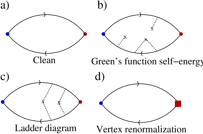
Figure 9: (a): Feynman diagram (“bubble”) representing the conductance tensor computed n the absence of impurity effects. (b): Sketch of the typical diagrams contributing to the self-energy renormalization (finite $\tau_{\rm Imp}^{-1}$). (c): Sketch of typical diagrams (“ladder”) contributing to the vertex renormalization. (d): Pictorial representation of the renormalization of the spin-hall current vertex (red square).

In principle the inverse lifetime $\tau_{\rm Imp}^{\lambda}$ (that is, the imaginary part of the single-electron self-energy) should be computed separately for each band. To second order in the impurity interaction strength, it is determined by the condition

$$\frac{1}{2\tau_{\rm Imp}^{\lambda}}=-\frac{N_{\rm Imp}\>\bar{u}^{2}}{V}\>\sum_{\vec{q}}\>\sum_{\mu}\times$$

$$\{{\cal A}_{(\vec{k},\lambda);(\vec{q},\mu)}\>{\cal A}_{(\vec{q},\mu);(\vec{k},\lambda)}\>\Im m\{g_{(\vec{q},\mu)}^{R;(0)}(\omega)\}\}\>\>\>\>.$$ (46)

Substituting, in the right-hand side of Eq.(46), $g_{(\vec{q},\mu)}^{R;(0)}(\omega)$ with $g_{(\vec{q},\mu)}^{R}(\omega)$ yields a set of self-consistent equations for the $\tau_{\rm Imp}^{\lambda}$. In general, solving, even numerically, the full set of equations is quite a formidable task to achieve, especially because, due to the dependence on the momenta of ${\cal A}_{(\vec{k},\lambda);(\vec{q},\mu)}$, one cannot exclude a priori an explicit dependence of $\tau_{\rm Imp}^{\lambda}$ on the momentum $\vec{k}$, as well. This eventually reflects into the formulas for the response functions, with a corresponding substantial increase in the computational complexity of the problem. For this reason it is compelling to find pertinent approximations that might possibly simplify the calculation of the imaginary part of the single-particle self-energy. In some cases, such as in the two-band Rashba model, the calculation simplifies with no further approximations, due to the fact that summing over $\vec{q}$ allows for $\tau_{\rm Imp}$ fully getting rid of any dependence on both $\vec{k}$ and $\lambda$ (see Appendix C for details). In the eight-band model the situation is not so simple and, as we discuss in the following, we have to resort to some “educated” approximations to make our problem tractable.

B.2 Impurity induced vertex renormalization

To derive the impurity induced vertex renormalization, we consider the diagrams contributing a specific conductance tensor in the absence of impurity effects, such as the “bubble” diagram reported in Fig. 9(a), with the colored dots representing the vertex insertions respectively corresponding to the operator coupled to the external source field (blue dot, in our formalism this corresponds to $[j_{{\rm ch},a}]_{(\vec{k},\lambda);(\vec{k}^{\prime},\lambda^{\prime})}$), and the vertex insertion represented by the red dot corresponding to the specific operator that we measure (in our case this corresponds to $[{\cal O}_{1}]_{(\vec{k},\lambda);(\vec{k}^{\prime},\lambda^{\prime})}$). Next, we “dress” the retarded and the advanced single-particle Green’s functions with the self-energy corrections described in the previous subsection. Diagrammatically, this amounts to adding to the “bare” bubble the contributions of diagrams such as the ones sketched in Fig. 9(b). Finally, we introduce diagrams such as the ones in Fig. 9(c), which renormalize the vertices, as well. Carefully doing the calculation and singling out only the total contributions arising from diagrams such as those in Fig. 9(c), it is possible to recover the corresponding contribution to the fermion bubble that yields the required vertex renormalization. For a generic pair of bilinear operators in the fermionic fields, ${\cal O}_{1}(\vec{r},t)$ and ${\cal O}_{2}(\vec{r}^{\prime},t^{\prime})$, we have therefore to recover the vertex renormalization from the retarded Green’s function $\theta(t-t^{\prime})\>\langle[{\cal O}_{1}(\vec{r},t),{\cal O}_{2}(\vec{r}^{\prime},t^{\prime})]\rangle$.

We now consider the impurity-induced renormalization of the equal-momentum vertex corresponding to an insertion of a generic operator ${\cal O}_{1}(\vec{r},t)$. Taking into account the impurity-induced imaginary part of the self-energy, we obtain the modified version of Eq.(25) in the presence of a finite density of impurities, that is

$$\Sigma_{1,2}=\lim_{\omega_{0}\to 0}\sum_{a=\pm 1}\frac{a}{2\omega_{0}}\Biggl{\{}\frac{1}{V}\>\sum_{\vec{k}}\>\sum_{\lambda,\lambda^{\prime}}\>\int\>\frac{d\bar{\omega}}{2\pi}\>[{\cal O}_{1}]_{(\vec{k},\lambda);(\vec{k},\lambda^{\prime})}[{\cal O}_{2}]_{(\vec{k},\lambda^{\prime});(\vec{k},\lambda)}\times$$

$$\left\{f(\bar{\omega})[g_{(\vec{k},\lambda)}^{R}(\bar{\omega)}-g_{(\vec{k},\lambda)}^{A}(\bar{\omega)}]g_{(\vec{k},\lambda^{\prime})}^{R}(\bar{\omega}+a\omega_{0})+f(\bar{\omega}+a\omega_{0})g_{(\vec{k},\lambda)}^{A}(\bar{\omega})[g_{(\vec{k},\lambda^{\prime})}^{R}(\bar{\omega}+a\omega_{0})-g_{(\vec{k},\lambda^{\prime})}^{A}(\bar{\omega}+a\omega_{0})]\right\}$$

$$+\frac{1}{V}\>\sum_{\vec{k}}\>\sum_{\lambda,\lambda^{\prime}}\>\int\>\frac{d\bar{\omega}}{2\pi}\>[\delta{\cal O}_{1}]_{(\vec{k},\lambda);(\vec{k},\lambda^{\prime})}^{(\bar{\omega},\bar{\omega}+a\omega_{0});[R,R]}[{\cal O}_{2}]_{(\vec{k},\lambda^{\prime});(\vec{k},\lambda)}\>f(\bar{\omega})g_{(\vec{k},\lambda)}^{R}(\bar{\omega)}g_{(\vec{k},\lambda^{\prime})}^{R}(\bar{\omega}+a\omega_{0})$$

$$-\frac{1}{V}\>\sum_{\vec{k}}\>\sum_{\lambda,\lambda^{\prime}}\>\int\>\frac{d\bar{\omega}}{2\pi}\>[\delta{\cal O}_{1}]_{(\vec{k},\lambda);(\vec{k},\lambda^{\prime})}^{(\bar{\omega},\bar{\omega}+a\omega_{0});[A,A]}[{\cal O}_{2}]_{(\vec{k},\lambda^{\prime});(\vec{k},\lambda)}\>f(\bar{\omega}+\omega_{0})g_{(\vec{k},\lambda)}^{A}(\bar{\omega)}g_{(\vec{k},\lambda^{\prime})}^{A}(\bar{\omega}+a\omega_{0})$$

$$+\frac{1}{V}\>\sum_{\vec{k}}\>\sum_{\lambda,\lambda^{\prime}}\>\int\>\frac{d\bar{\omega}}{2\pi}\>[\delta{\cal O}_{1}]_{(\vec{k},\lambda);(\vec{k},\lambda^{\prime})}^{(\bar{\omega},\bar{\omega}+a\omega_{0});[A,R]}[{\cal O}_{2}]_{(\vec{k},\lambda^{\prime});(\vec{k},\lambda)}\>[f(\bar{\omega}+a\omega_{0})-f(\bar{\omega})]g_{(\vec{k},\lambda)}^{A}(\bar{\omega)}g_{(\vec{k},\lambda^{\prime})}^{R}(\bar{\omega}+a\omega_{0})\Biggr{\}}\;\;\;\;,$$ (47)

with the vertex correction $[\delta{\cal O}_{1}]_{(\vec{k},\lambda);(\vec{k},\lambda^{\prime})}^{(\bar{\omega},\bar{\omega}+\omega_{0});[X,Y]}$ ($X,Y=A,R$) satisfying the equation

$$[\delta{\cal O}_{1}]_{(\vec{k},\lambda);(\vec{k},\lambda^{\prime})}^{(\bar{\omega},\bar{\omega}+\omega_{0});[X,Y]}=\sum_{n=1}^{\infty}\{[\delta{\cal O}_{1}]_{(\vec{k},\lambda);(\vec{k},\lambda^{\prime})}^{(\bar{\omega},\bar{\omega}+\omega_{0});[X,Y]}\}_{(n)}\;\;\;\;,$$ (48)

with

$$\{[\delta{\cal O}_{1}]_{(\vec{k},\lambda);(\vec{k},\lambda^{\prime})}^{(\bar{\omega},\bar{\omega}+\omega_{0});[X,Y]}\}_{(1)}=\frac{\bar{u}^{2}N_{\rm Imp}}{V}\>\sum_{\vec{q}}\;\sum_{\mu,\mu^{\prime}}{\cal A}_{(\vec{k},\lambda);(\vec{q},\mu)}\times$$

$$g_{(\vec{q},\mu)}^{X}(\bar{\omega})[{\cal O}_{1}]_{(\vec{q},\mu);(\vec{q},\mu^{\prime})}g_{(\vec{q},\mu^{\prime})}^{Y}(\bar{\omega}+\omega_{0})\>{\cal A}_{(\vec{q},\mu^{\prime});(\vec{k},\lambda^{\prime})}\;,$$ (49)

and

$$\{[\delta{\cal O}_{1}]_{(\vec{k},\lambda);(\vec{k},\lambda^{\prime})}^{(\bar{\omega},\bar{\omega}+\omega_{0});[X,Y]}\}_{(n+1)}=$$ (50)

$$\frac{\bar{u}^{2}N_{\rm Imp}}{V}\>\sum_{\vec{q}}\;\sum_{\mu,\mu^{\prime}}\>{\cal A}_{(\vec{k},\lambda);(\vec{q},\mu)}g_{(\vec{q},\mu)}^{X}(\bar{\omega})\times$$

$$\{[\delta{\cal O}_{1}]_{(\vec{q},\mu);(\vec{q},\mu^{\prime})}^{(\bar{\omega},\bar{\omega}+\omega_{0});[X,Y]}\}_{(n)}g_{(\vec{q},\mu^{\prime})}^{Y}(\bar{\omega}+\omega_{0})\>{\cal A}_{(\vec{q},\mu^{\prime});(\vec{k},\lambda^{\prime})}\;\;\;\;.$$

To formally solve the iterative system in Eqs.(49) and (50), we set

$$\{[\delta{\cal O}_{1}]_{(\sigma);(\sigma^{\prime})}^{(\bar{\omega},\bar{\omega}+\omega_{0});[X,Y]}\}_{(n)}=$$ (51)

$$\sum_{\vec{k}}\>\sum_{\lambda,\lambda^{\prime}}[w^{\vec{k}}_{\sigma,\lambda}]^{*}w_{\sigma^{\prime},\lambda^{\prime}}^{\vec{k}}\{[\delta{\cal O}_{1}]_{(\sigma,\sigma^{\prime})}^{(\bar{\omega},\bar{\omega}+\omega_{0});[X,Y]}\}_{(n)}\;,$$

which enables us to respectively rewrite Eqs.(49) and Eqs.(50) in the form

$$\{[\delta{\cal O}_{1}]_{(\sigma,\sigma^{\prime})}^{(\bar{\omega},\bar{\omega}+\omega_{0});[X,Y]}\}_{(1)}=\frac{\bar{u}^{2}N_{\rm Imp}}{V}\>\sum_{\vec{q}}\;\sum_{\sigma_{1},\sigma_{1}^{{}^{\prime}}}\times$$

$$g_{[\vec{q};(\sigma,\sigma_{1})]}^{X}(\bar{\omega})[{\cal O}_{1}]_{(\sigma_{1},\sigma_{1}^{{}^{\prime}})}g_{[\vec{q};(\sigma_{1}^{{}^{\prime}},\sigma^{\prime})]}^{Y}(\bar{\omega}+\omega_{0})\;\;\;\;,$$ (52)

and

$$\{[\delta{\cal O}_{1}]_{(\sigma,\sigma^{\prime})}^{(\bar{\omega},\bar{\omega}+\omega_{0});[X,Y]}\}_{(n+1)}=\frac{\bar{u}^{2}N_{\rm Imp}}{V}\>\sum_{\vec{q}}\;\sum_{\sigma_{1},\sigma_{1}^{{}^{\prime}}}\times$$ (53)

$$g_{[\vec{q};(\sigma,\sigma_{1})]}^{X}(\bar{\omega})\{[\delta{\cal O}_{1}]_{(\sigma_{1},\sigma_{1}^{{}^{\prime}})}^{(\bar{\omega},\bar{\omega}+\omega_{0});[X,Y]}\}_{(n)}g_{[\vec{q};(\sigma_{1}^{{}^{\prime}},\sigma^{\prime})]}^{Y}(\bar{\omega}+\omega_{0})\ \;\;,$$

with

$$g_{[\vec{q};(\sigma,\sigma^{\prime})]}^{X}(\bar{\omega})=\sum_{\lambda}\>w^{\vec{q}}_{\sigma,\lambda}[w^{\vec{q}}_{\sigma^{\prime},\lambda}]^{*}\>g^{X}_{(\vec{q},\lambda)}(\bar{\omega})\>\>\>\>.$$ (54)

As a further formal simplification, we only retain the vertex corrections at the right-hand side of Eq. (47) containing the $[A,R]$-terms Dimitrova (2005). Accordingly we eventually obtain the vertex-correction induced additional contribution to $\Sigma_{1,2}$, $\delta\Sigma_{1,2}$, given by (in the zero-temperature limit)

$$\delta\Sigma_{1,2}=\frac{1}{V}\sum_{\vec{k}}\sum_{\lambda,\lambda^{\prime}}\>\int\frac{d\bar{\omega}}{2\pi}\times$$ (55)

$$[\delta{\cal O}_{1}]_{(\vec{k},\lambda);(\vec{k},\lambda^{\prime})}^{(\bar{\omega},\bar{\omega});[A,R]}[{\cal O}_{2}]_{(\vec{k},\lambda^{\prime});(\vec{k},\lambda)}g^{A}_{(\vec{k},\lambda)}(\bar{\omega})g^{R}_{(\vec{k},\lambda^{\prime})}(\bar{\omega})\partial_{\bar{\omega}}f(\bar{\omega})=$$

$$-\frac{2\pi}{V}\sum_{\vec{k}}\sum_{\lambda,\lambda^{\prime}}\>[\delta{\cal O}_{1}]_{(\vec{k},\lambda);(\vec{k},\lambda^{\prime})}^{(0,0);[A,R]}[{\cal O}_{2}]_{(\vec{k},\lambda^{\prime});(\vec{k},\lambda)}g^{A}_{(\vec{k},\lambda)}(0)g^{R}_{(\vec{k},\lambda^{\prime})}(0)\>\>\>\>.$$

Appendix C Spin-Hall conductance in a lattice model for the two-dimensional Rashba Hamiltonian

As a test bed of our approach, in this appendix we compute the SHC in a lattice model for a two-dimensional electron gas with Rashba SOI, described by the Hamiltonian $H_{\rm R}$ given by

$$H_{\rm R}=\frac{1}{V}\>\sum_{\vec{k}}\>\sum_{\sigma,\sigma^{\prime}}c_{\vec{k},\sigma}^{\dagger}[{\cal H}_{\rm R}(\vec{k})]_{\sigma,\sigma^{\prime}}c_{\vec{k},\sigma^{\prime}}\>\>\>\>,$$ (56)

with $V$ being the (two-dimensional) lattice “volume”, $\sigma$ and $\sigma^{\prime}$ being actual spin labels, and

$${\cal H}_{\rm R}(\vec{k})=\left[\begin{array}[]{cc}\epsilon_{\vec{k}}&\delta_{\vec{k}}\\ \delta^{*}_{\vec{k}}&\epsilon_{\vec{k}}\end{array}\right]\;\;\;\;,$$ (57)

with

$$\epsilon_{\vec{k}} = -2t\{\cos(k_{x})+\cos(k_{y})\}\;,$$

$$\delta_{\vec{k}} = 2\alpha\{i\sin(k_{x})+\sin(k_{y})\}\>.$$ (58)

The relevant parameters of $H_{\rm R}$ are the single-fermion hopping amplitude $t$ (which we assume to be the same both along the $x$ and $y$ directions over the lattice) and the Rashba spin-orbit coupling $\alpha$. Eventually, we use the chemical potential $\mu$ as our tuning parameter.

To compute the SHC we need the SH current and the charge-current operators, respectively given by (in the $2\times 2$ matrix notation)

$$j_{{\rm sp},x}^{z} = t\sin(k_{x})\sigma^{z}\;\;,$$

$$j_{{\rm ch},y} = 2et\sin(k_{y}){\bf I}+2e\alpha\cos(k_{y})\sigma^{x}\;\;\;\;.$$ (59)

The energy eigenvalues, $\epsilon_{\vec{k},\lambda}$, with $\lambda=\pm$, and the corresponding eigenmodes $\Gamma_{\vec{k},\lambda}$ are given by

$$\epsilon_{\vec{k},\lambda}=\epsilon_{\vec{k}}+\lambda|\delta_{\vec{k}}|\;\;\;\;,$$ (60)

and by

$$\Gamma_{\vec{k},+} = \frac{1}{\sqrt{2}}\{c_{\vec{k},\uparrow}+e^{i\varphi_{\vec{k}}}c_{\vec{k},\downarrow}\}\;,$$

$$\Gamma_{\vec{k},-} = \frac{1}{\sqrt{2}}\{-e^{-i\varphi_{\vec{k}}}c_{\vec{k},\uparrow}+c_{\vec{k},\downarrow}\}\;,$$ (61)

with $\varphi_{\vec{k}}={\rm arg}(\delta_{\vec{k}})$. Once rotated to the energy eigenmode basis, the operators in Eq.(59) become

$$j_{{\rm sp},x}^{z} \to -t\sin(k_{x})\{\cos(\varphi_{\vec{k}})\sigma^{x}-\sin(\varphi_{\vec{k}})\sigma^{y}\}\;,$$ (62)

$$j_{{\rm ch},y} \to 2et\sin(k_{y}){\bf I}+2e\alpha\cos(k_{y})\cos(\varphi_{\vec{k}})\sigma^{z}$$

$$- 2e\alpha i\sin(\varphi_{\vec{k}})\cos(k_{y})\{\cos(\varphi_{\vec{k}})\sigma^{x}-\sin(\varphi_{\vec{k}})\sigma^{y}\}\;.$$

Summing over the possible directions of $\vec{k}$ (within the Brillouin zone) allows for rewriting Eq.(46) as

$$1=\frac{N_{\rm Imp}\bar{u}^{2}}{2V}\>\sum_{\vec{k}}\sum_{\lambda=\pm 1}\left\{\frac{1}{(\epsilon_{\vec{k}}+\lambda|\delta_{\vec{k}}|-\mu)^{2}+(2\tau_{\rm Imp})^{-2}}\right\}\>\>\>\>.$$ (63)

From Eq.(63) we see that any dependence on the momentum, as well as on the spin index, has disappeared at the right-hand side of the equation, leaving only an over-all factor of $\frac{1}{2}$. While, this is just a special feature of the two-band Rashba model, it is in any case a useful guideline to choosing the appropriate approximations to implement in the more complicated multiband calculation.

We now compute the SHC of the two-band Rashba model, $\sigma_{xy}^{z}$. To do so, we label with subscript $1$ the vertex corresponding to the $z$-component of the spin current along $x$ and with subscript $2$ the vertex corresponding to the charge current along $y$. As in the main text, we denote with $\sigma_{xy;A}^{z}$ the contribution to the SHC without vertex corrections and with $\sigma_{xy;B}^{z}$ the total contribution arising from vertex corrections. As a next step, we consider the splitting in Eqs.(26), which in this case yields

$$[{\cal S}_{1,2}]_{(\vec{k},\lambda);(\vec{k},\lambda^{\prime})} = 0\;\;,\;\forall\lambda,\lambda^{\prime}\;,$$

$${}_{(\vec{k},+);(\vec{k},+)} = [{\cal I}_{1,2}]_{(\vec{k},-);(\vec{k},-)}=0\;,$$

$${}_{(\vec{k},+);(\vec{k},-)} = -[{\cal I}_{1,2}]_{(\vec{k},-);(\vec{k},+)}=$$ (64)

$$\frac{2et\alpha\sin^{2}(k_{x})\cos(k_{y})}{\sqrt{\sin^{2}(k_{x})+\sin^{2}(k_{y})}}\>\>\>\>.$$

Taking into account Eqs.(64), we obtain

$$\sigma_{xy;A}^{z}=\frac{2et\alpha}{\pi V}\>\sum_{\vec{k}}\frac{\sin^{2}(k_{x})\cos(k_{y})\Phi_{\vec{k}}(\mu)}{\sqrt{\sin^{2}(k_{x})+\sin^{2}(k_{y})}}\;\;\;\;,$$ (65)

with

$$\Phi(\mu) = -i\int_{-\infty}^{0}\frac{d\bar{\omega}}{2\pi}\>\sum_{\lambda=\pm}\lambda[g_{(\vec{k},\lambda)}^{A}(\bar{\omega})-g_{(\vec{k},\lambda)}^{R}(\bar{\omega})]\partial_{\bar{\omega}}[g_{(\vec{k},-\lambda)}^{A}(\bar{\omega})+g_{(\vec{k},-\lambda)}^{R}(\bar{\omega})]$$ (66)

$$= \frac{2\tau_{\rm Imp}[(|\delta_{\vec{k}}|^{2}-(\epsilon_{\vec{k}}-\mu)^{2})-(2\tau_{\rm Imp})^{-2}]}{\pi|\delta_{\vec{k}}|\{(2\tau_{\rm Imp})^{-2}+2[(\epsilon_{\vec{k}}-\mu)^{2}+|\delta_{\vec{k}}|^{2}+2\tau_{\rm Imp}^{2}((\epsilon_{\vec{k}}-\mu)^{2}-|\delta_{\vec{k}}|^{2})^{2}]\}}$$

$$+ \left\{\frac{{\rm arctan}[2\tau_{\rm Imp}(|\delta_{\vec{k}}|-\epsilon_{\vec{k}}+\mu)]+{\rm arctan}[2\tau_{\rm Imp}(|\delta_{\vec{k}}|+\epsilon_{\vec{k}}-\mu)]}{2\pi|\delta_{\vec{k}}|^{2}}\right\}\>\>\>\>.$$

The contribution determined by the vertex corrections, $\sigma_{xy;B}^{z}$, can be computed according to Eq.(55). It is given by

$$\sigma_{xy;B}^{z} = \frac{2}{\pi V}\sum_{\vec{k}}\sum_{\sigma,\sigma^{\prime}}\sum_{\rho,\rho^{\prime}}[\delta j_{{\rm sp},x}^{z}]^{(0,0);[A,R]}_{(\vec{k},\sigma);(\vec{k},\sigma^{\prime})}\times$$ (67)

$$g_{\vec{k};(\rho,\sigma)}^{A}(0)g_{\vec{k};(\sigma^{\prime},\rho^{\prime})}^{R}(0)[j_{{\rm ch},y}]_{(\vec{k},\rho^{\prime});(\vec{k},\rho)}\>.$$

(Note that, for computational purposes, we wrote Eq.(67) in the spin-eigenstate basis). Finally, going through the systematic procedure discussed in appendix B, we find for the renormalized vertex the expression

$$[\delta j_{{\rm sp},x}^{z}]^{(0,0);[A,R]}_{(\vec{k},\sigma);(\vec{k},\sigma^{\prime})}=\frac{N_{\rm Imp}\bar{u}^{2}\Lambda}{1-N_{\rm Imp}\bar{u}^{2}\nu}[\sigma^{x}]_{\sigma,\sigma^{\prime}}\;\;\;\;,$$ (68)

that is independent of $\vec{k}$, with

$$\Lambda = \frac{\alpha t}{\tau_{\rm Imp}V}\sum_{\vec{q}}\left\{\frac{\sin^{2}(q_{x})}{(2\tau_{\rm Imp})^{-4}+2(2\tau_{\rm Imp})^{-2}[(\epsilon_{\vec{q}}-\mu)^{2}+|\delta_{\vec{q}}|^{2}]+[(\epsilon_{\vec{q}}-\mu)^{2}-|\delta_{\vec{q}}|^{2}]^{2}}\right\}\;,$$

$$\nu = \frac{1}{V}\sum_{\vec{q}}\left\{\frac{(\epsilon_{\vec{q}}-\mu)^{2}+(2\tau_{\rm Imp})^{-2}}{(2\tau_{\rm Imp})^{-4}+2(2\tau_{\rm Imp})^{-2}[(\epsilon_{\vec{q}}-\mu)^{2}+|\delta_{\vec{q}}|^{2}]+[(\epsilon_{\vec{q}}-\mu)^{2}-|\delta_{\vec{q}}|^{2}]^{2}}\right\}\>\>\>\>.$$ (69)

Finally, plugging Eq. (63) into (68), we eventually get

$$[\delta j_{{\rm sp},x}^{z}]^{(0,0);[A,R]}_{(\vec{k},\sigma);(\vec{k},\sigma^{\prime})}=\frac{t}{4\alpha\tau_{\rm Imp}}\sigma^{x}\>\>\>\>.$$ (70)

Inserting Eq. (70) into (67), we derive $\sigma_{xy;B}^{z}$ as a function of $\mu$.

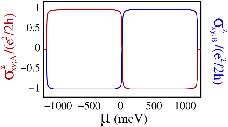
Figure 10: Contributions to the spin-Hall conductance $\sigma_{xy;A}^{z}$ (red curve) and $\sigma_{xy;B}^{z}$ (blue curve) in the model described by the lattice Rashba Hamiltonian in Eq. (56), in the presence of a finite impurity concentration, with parameters chosen so that $t=300{\rm meV}$, $\alpha=10{\rm meV}$ and $\tau_{\rm Imp}=3{\rm ps}$.

In Fig. 10 we separately plot the results for the two terms, computed using the Hamiltonian $H_{\rm R}$ with t=300 meV, $\alpha=10\;{\rm meV}$ and with $\tau_{\rm Imp}=3\;{\rm ps}$. From the plot in Fig. 10 we note the main features of the SHC in a Rashba-2DEG in the presence of impurity. First, we note that, in the absence of vertex corrections, $\sigma_{xy}^{z}$ is either zero, or it is quantized (in units of $e^{2}/2h$) Kane and Mele (2005). When including vertex corrections, these fully screen the SHC, which results in the absence of the effect, as widely discussed in the literature Rashba (2004); Mishchenko et al. (2004); Inoue et al. (2004); Khaetskii (2006); Raimondi and Schwab (2005); Dimitrova (2005); Shytov et al. (2006). In the main text we, instead, note how the behavior is completely different in the multiband model, due to the various, impurity induced, interband processes. This notwithstanding the fact that, as we show in the next appendix, at low enough values of $\mu$, the 8-band model can be effectively described as a Rashba-like Hamiltonian such as the one we discuss here.

Appendix D Effective two-subband Rashba-like Hamiltonian

In this appendix we show how the eight-band model of Sec. III, when $\mu$ is within the first pair of subbands but still below the bottom of higher-energy subbands, can be effectively described by a Rashba Hamiltonian $H_{\rm xy}$, involving the effects of virtual transitions from the low-lying subbands to, and from, higher-energy bands.

Employing the approach developed in Ref.Lepori et al. (2021) and referring to the eight-band Hamiltonian that we discuss in Sec. III, we define the energy eigenmodes $\Gamma_{\vec{k},\lambda}$ as $\Gamma_{\vec{k},\lambda}=\sum_{\alpha}\sum_{s}u_{\alpha,s}^{*}c_{\alpha,s}$, with $\alpha\in\{(xy;A),(xy;B),zx,yz\}$ and $s$ being the spin polarization. In the following, we will simply denote with $u_{\alpha}$ the (bi)spinor $[u_{\alpha,\uparrow},u_{\alpha,\downarrow}]_{t}$. We now recover the reduced, effective Hamiltonian for the first two subbands in the bispinor representation, by systematically going through a projection over the $xy;A$ and the $xy;B$ subbands. To do so, we introduce the projection operators ${\cal P}$ and ${\cal Q}$ which, in the block notation of Sec. III and in the basis of the spinors such as the one in Eq.(8) are written as

$${\cal P}=\left[\begin{array}[]{cccc}{\bf 0}&{\bf 0}&{\bf 0}&{\bf 0}\\ {\bf 0}&{\bf 0}&{\bf 0}&{\bf 0}\\ {\bf 0}&{\bf 0}&{\bf I}&{\bf 0}\\ {\bf 0}&{\bf 0}&{\bf 0}&{\bf I}\end{array}\right]\;\;\;,\;{\cal Q}=\left[\begin{array}[]{cccc}{\bf I}&{\bf 0}&{\bf 0}&{\bf 0}\\ {\bf 0}&{\bf I}&{\bf 0}&{\bf 0}\\ {\bf 0}&{\bf 0}&{\bf 0}&{\bf 0}\\ {\bf 0}&{\bf 0}&{\bf 0}&{\bf 0}\end{array}\right]\>\>\>\>.$$ (71)

Projecting with ${\cal P}$ and ${\cal Q}$ the Schrödinger equation corresponding to the Hamiltonian in Eq.(9), we obtain

$$\left[\begin{array}[]{cc}\epsilon-\epsilon_{xy;A}(\vec{k})&{\bf 0}\\ {\bf 0}&\epsilon-\epsilon_{xy;B}(\vec{k})\end{array}\right]\left[\begin{array}[]{c}u_{xy;A}\\ u_{xy;B}\end{array}\right]=i\left[\begin{array}[]{cc}f_{1}^{X}(\vec{k})+\lambda_{\rm SOI}\sigma^{y}&f_{1}^{Y}(\vec{k})-\lambda_{\rm SOI}\sigma^{x}\\ f_{2}^{X}(\vec{k})+\lambda_{\rm SOI}\sigma^{y}&f_{2}^{Y}(\vec{k})-\lambda_{\rm SOI}\sigma^{x}\end{array}\right]\left[\begin{array}[]{c}u_{yz}(\vec{k})\\ u_{zx}(\vec{k})\end{array}\right]$$ (80)

$$\left[\begin{array}[]{cc}\epsilon-\epsilon_{yz}(\vec{k})&-i\lambda_{\rm SOI}\sigma^{z}\\ i\lambda_{\rm SOI}\sigma^{z}&\epsilon-\epsilon_{zx}(\vec{k})\end{array}\right]\left[\begin{array}[]{c}u_{yz}(\vec{k})\\ u_{zx}(\vec{k})\end{array}\right]=-i\left[\begin{array}[]{cc}f_{1}^{X}(\vec{k})+\lambda_{\rm SOI}\sigma^{y}&f_{2}^{X}(\vec{k})+\lambda_{\rm SOI}\sigma^{y}\\ f_{1}^{Y}(\vec{k})-\lambda_{\rm SOI}\sigma^{x}&f_{2}^{Y}(\vec{k})-\lambda_{\rm SOI}\sigma^{x}\end{array}\right]\left[\begin{array}[]{c}u_{xy;A}\\ u_{xy;B}\end{array}\right]\>\>\>\>.$$ (89)

Getting rid of the $u_{yz}(\vec{k})$ and of the $u_{zx}(\vec{k})$, Eqs.(89) yields the reduced time-independent Schrödinger equation, with energy eigenvalue $\epsilon$, projected over the low-lying doublets in the form

$$\left[\begin{array}[]{cc}\epsilon-\epsilon_{xy;A}(\vec{k})-h_{AA}(\vec{k})&-h_{AB}(\vec{k})\\ -h_{BA}(\vec{k})&\epsilon-\epsilon_{xy;B}(\vec{k})-h_{BB}(\vec{k})\end{array}\right]\left[\begin{array}[]{c}u_{xy;A}(\vec{k})\\ u_{xy;B}(\vec{k})\end{array}\right]=0\>\>\>\>,$$ (90)

with

$$\left[\begin{array}[]{cc}h_{AA}(\vec{k})&h_{AB}(\vec{k})\\ h_{BA}(\vec{k})&h_{BB}(\vec{k})\end{array}\right]=\frac{1}{[\epsilon-\epsilon_{yz}(\vec{k})][\epsilon-\epsilon_{zx}(\vec{k})]-\lambda_{\rm SOI}^{2}}\>\left[\begin{array}[]{cc}f_{1}^{X}(\vec{k})+\lambda_{\rm SOI}\sigma^{y}&f_{1}^{Y}(\vec{k})-\lambda_{\rm SOI}\sigma^{x}\\ f_{2}^{X}(\vec{k})+\lambda_{\rm SOI}\sigma^{y}&f_{2}^{Y}(\vec{k})-\lambda_{\rm SOI}\sigma^{x}\end{array}\right]\times$$ (95)

$$\left[\begin{array}[]{cc}\epsilon-\epsilon_{zx}(\vec{k})&i\lambda\sigma^{z}\\ -i\lambda\sigma^{z}&\epsilon-\epsilon_{yz}(\vec{k})\end{array}\right]\left[\begin{array}[]{cc}f_{1}^{X}(\vec{k})+\lambda_{\rm SOI}\sigma^{y}&f_{2}^{X}(\vec{k})+\lambda_{\rm SOI}\sigma^{y}\\ f_{1}^{Y}(\vec{k})-\lambda_{\rm SOI}\sigma^{x}&f_{2}^{Y}(\vec{k})-\lambda_{\rm SOI}\sigma^{x}\end{array}\right]\left[\begin{array}[]{c}u_{xy;A}\\ u_{xy;B}\end{array}\right]\>\>\>\>.$$ (102)

Explicitly expanding the right-hand side of Eq.(102), we eventually obtain

$$h_{AA}(\vec{k})={\cal D}^{-1}(\vec{k})\Biggl{\{}(\epsilon-\epsilon_{zx}(\vec{k}))[f_{2}^{X}(\vec{k})]^{2}+(\epsilon-\epsilon_{yz}(\vec{k}))[f_{2}^{Y}(\vec{k})]^{2}+\lambda_{\rm SOI}^{2}\>[2\epsilon-\epsilon_{zx}(\vec{k})-\epsilon_{yz}(\vec{k})]$$ (103)

$$+2\lambda_{\rm SOI}\>\{-(\epsilon-\epsilon_{yz}(\vec{k}))f_{1}^{Y}(\vec{k})\sigma^{x}+(\epsilon-\epsilon_{zx}(\vec{k}))f_{1}^{X}(\vec{k})\sigma^{y}\}\Biggr{\}}$$

$$h_{BB}(\vec{k})={\cal D}^{-1}(\vec{k})\Biggl{\{}(\epsilon-\epsilon_{zx}(\vec{k}))[f_{1}^{X}(\vec{k})]^{2}+(\epsilon-\epsilon_{yz}(\vec{k}))[f_{1}^{Y}(\vec{k})]^{2}+\lambda_{\rm SOI}^{2}\>[2\epsilon-\epsilon_{zx}(\vec{k})-\epsilon_{yz}(\vec{k})]$$

$$+2\lambda_{\rm SOI}\>\{-(\epsilon-\epsilon_{yz}(\vec{k}))f_{2}^{Y}(\vec{k})\sigma^{x}+(\epsilon-\epsilon_{zx}(\vec{k}))f_{2}^{X}(\vec{k})\sigma^{y}\}\Biggr{\}}$$

$$h_{AB}(\vec{k})=h_{BA}^{*}(\vec{k})=$$

$${\cal D}^{-1}(\vec{k})\Biggl{\{}(\epsilon-\epsilon_{zx}(\vec{k}))(f_{1}^{X}(\vec{k})+\lambda_{\rm SOI}\sigma^{y})(f_{2}^{X}(\vec{k})+\lambda_{\rm SOI}\sigma^{y})+(\epsilon-\epsilon_{yz}(\vec{k}))(f_{1}^{Y}(\vec{k})-\lambda_{\rm SOI}\sigma^{x})(f_{2}^{Y}(\vec{k})-\lambda_{\rm SOI}\sigma^{x})$$

$$+i\lambda_{\rm SOI}\{-(\epsilon-\epsilon_{zx}(\vec{k}))(f_{1}^{Y}(\vec{k})-\lambda_{\rm SOI}\sigma^{x})(f_{2}^{X}(\vec{k})+\lambda_{\rm SOI}\sigma^{y})+(\epsilon-\epsilon_{yz}(\vec{k}))(f_{1}^{X}(\vec{k})+\lambda_{\rm SOI}\sigma^{y})(f_{2}^{Y}(\vec{k})-\lambda_{\rm SOI}\sigma^{x})\}\sigma^{z}\Biggr{\}}\>\>\>\>,$$

with

$${\cal D}^{-1}(\vec{k})=\frac{1}{[\epsilon-\epsilon_{yz}(\vec{k})][\epsilon-\epsilon_{zx}(\vec{k})]-\lambda_{\rm SOI}^{2}}\>\>\>\>.$$ (104)

At a given chemical potential $\mu$, for $-\Delta_{A}<\mu<-\Delta_{B}$ we approximate the matrix elements in Eqs. (103) by simply substituting $\epsilon$ with $\epsilon_{xy;A}(\vec{k})$. For $|\mu|\sim\Delta_{A}$ we may further neglect the effective inter-band couplings in the right-hand side of Eqs. (102) and (103) by therefore introducing a simple effective Rashba-type Hamiltonian for the $xy;A$ doublet, $H_{AA}(\vec{k})$, given by

$$H_{\rm AA}(\vec{k}) = \epsilon_{xy;A}(\vec{k})+\{(\epsilon_{xy;A}(\vec{k})-\epsilon_{yz}(\vec{k}))(\epsilon_{xy;A}(\vec{k})-\epsilon_{zx}(\vec{k}))-\lambda_{\rm SOI}^{2}\}^{-2}\>\times$$ (105)

$$\biggl{\{}(\epsilon_{xy;A}(\vec{k})-\epsilon_{zx}(\vec{k}))[f_{2}^{X}(\vec{k})]^{2}+(\epsilon_{xy;A}(\vec{k})-\epsilon_{yz}(\vec{k}))[f_{2}^{Y}(\vec{k})]^{2}+\lambda_{\rm SOI}^{2}\>[2\epsilon_{xy;A}(\vec{k})-\epsilon_{zx}(\vec{k})-\epsilon_{yz}(\vec{k})]$$

$$+ 2\lambda_{\rm SOI}\>\biggl{[}-(\epsilon_{xy;A}(\vec{k})-\epsilon_{yz}(\vec{k}))f_{1}^{Y}(\vec{k})\sigma^{x}+(\epsilon_{xy;A}(\vec{k})-\epsilon_{zx}(\vec{k}))f_{1}^{X}(\vec{k})\sigma^{y}\biggr{]}\biggr{\}}\>\>\>\>.$$

Expanding the right-hand side of Eq.(105) up to second-order in $\vec{k}$, we obtain that $H_{AA}(\vec{k})\approx H_{xy}(\vec{k})$, with

$$H_{xy}(\vec{k})\approx-\hat{\Delta}_{A}+\hat{t}^{2}\vec{k}^{2}+\hat{\alpha}\{-k_{x}\sigma^{y}+k_{y}\sigma^{x}\}\;\;\;\;,$$ (106)

and

$$\hat{\Delta}_{A} = \Delta_{A}+\frac{2\Delta_{A}\lambda_{\rm SOI}^{2}}{\Delta_{A}^{2}-\lambda_{\rm SOI}^{2}}\;,$$

$$\hat{t} = t_{1}+\frac{\lambda_{\rm SOI}^{2}(t_{1}-t_{2})-4\Delta_{A}\gamma_{2}^{2}}{\Delta_{A}^{2}-\lambda_{\rm SOI}^{2}}-\frac{2\Delta_{A}^{2}\lambda_{\rm SOI}^{2}(t_{1}-t_{2})}{[\Delta_{A}^{2}-\lambda_{\rm SOI}^{2}]^{2}}\;,$$

$$\hat{\alpha} = \frac{4\gamma_{1}\lambda_{\rm SOI}\Delta_{A}}{\Delta_{A}^{2}-\lambda_{\rm SOI}^{2}}\>\>\>\>.$$ (107)

The emergence of an effective Hamiltonian, at low $\vec{k}$, with a linear Rashba spin-orbit coupling is consistent with the apparent suppression of the spin-Hall conductance due to the vertex renormalization in the low-$\mu$ part of the plot of Fig.7. Of course, on increasing $\mu$, nonlinear contributions to the Rashba coupling as well as inter-band terms in the system Hamiltonian are expected to spoil the perfect cancellation of the spin-Hall conductance from impurity-induced vertex corrections and, again, this is consistent with our result of Fig. 7.

Appendix E Analytical derivation of the sheet conductance and of the spin-Hall conductance in the 8-band model

In this appendix we provide the explicit derivation of the formulas for the sheet conductance and for the spin-Hall conductance in the eight-band model, that we used to analytically derive the plots that we show in the main text of the paper. All the formulas we derive in the following are grounded over a systematic implementation of the formalism that we review in Appendixes A and B. Before going through the details of the derivation of the conductances, it is crucial to extensively discuss and motivate the way in which we employ (the self-consistent version of) Eq.(46) for the inverse single-particle lifetime $\tau_{\rm Imp}^{\lambda}$.

In general, $\tau^{\lambda}_{\rm Imp}$ should be self-consistently determined from Eq.(46), with the “ bare” single-particle retarded Green’s function $g_{(\vec{q};\mu)}^{R;(0)}(\omega)$ at the right-hand side of the equation substituted with the “dressed” one $g_{(\vec{q};\mu)}^{R}(\omega)$ in Eq.(45). However, in the specific case of the LAO/STO interface, as it is evidenced in the Supplemental Material of Ref. Trier et al. (2020), within all the interval of values of the gate voltage that they consider (which corresponds to our interval of values of $\mu$), the elastic contribution to $\tau_{\rm Imp}$, $\tau_{\rm e}$, keeps smaller than the inelastic one, $\tau_{\rm i}$ (by even two to three orders of magnitude in the first part of the interval of values of $\mu$). This evidences how we can safely neglect $\tau_{\rm i}$ and, accordingly, compute $\tau_{\rm e}$ by setting to 0 the frequency $\omega$ in (the self-consistent version of) Eq. (46). Still keeping, for the time being, the explicit dependence on $\lambda$ we therefore simplify Eq.(46) to

$$\frac{1}{2\tau_{\rm e}^{\lambda}}=\frac{N_{\rm Imp}\bar{u}^{2}}{V}\sum_{\vec{q}}\sum_{\mu}\left[\frac{(2\tau_{\rm e}^{\mu})^{-1}{\cal A}_{(\vec{k},\lambda);(\vec{q},\mu)}{\cal A}_{(\vec{q},\mu);(\vec{k},\lambda)}}{\xi_{\vec{q},\mu}^{2}+(2\tau_{\rm e}^{\mu})^{-2}}\right]\>\>.$$ (108)

To recover a numerical estimate for the $\tau_{\rm e}^{\lambda}$, we rely on Ref. Trier et al. (2020), where the non-$\lambda$-resolved $\tau_{\rm e}$ is obtained from the measured magnetoconductance by means of a fit to the Maekawa-Fukuyama formula Huijben et al. (2017). Having only a band-independent estimate for $\tau_{\rm e}$ we dropped the dependence on $\lambda$ in the inverse lifetimes appearing at the right-hand side of Eq.(108) and approximated it by means of the rough estimate $\tau_{\rm e}\approx 3$ ps Trier et al. (2020). Accordingly dropping the dependence on $\lambda$ in $\tau_{\rm e}$ in Eq.(108), we further approximate it by averaging over $\lambda$, so that we eventually obtain

$$1=\frac{N_{\rm Imp}\bar{u}^{2}}{NV}\sum_{\vec{q}}\sum_{\mu}\left[\frac{1}{\xi_{\vec{q},\mu}^{2}+(2\tau_{\rm e})^{-2}}\right]\;\;\;\;.$$ (109)

While slightly changing the value of $\tau_{\rm e}$ and even adding a slight dependence on $\mu$ and/or on the band index $\lambda$ does almost not affect at all the contributions to the conductances from the nonzero, impurity induced single-fermion self energy. At variance, especially when computing $\sigma_{xy}^{z}$ in the multiband model, the implementation of the above approximations in computing the vertex corrections is crucial in determining the weight of that latter contribution on the finite result.

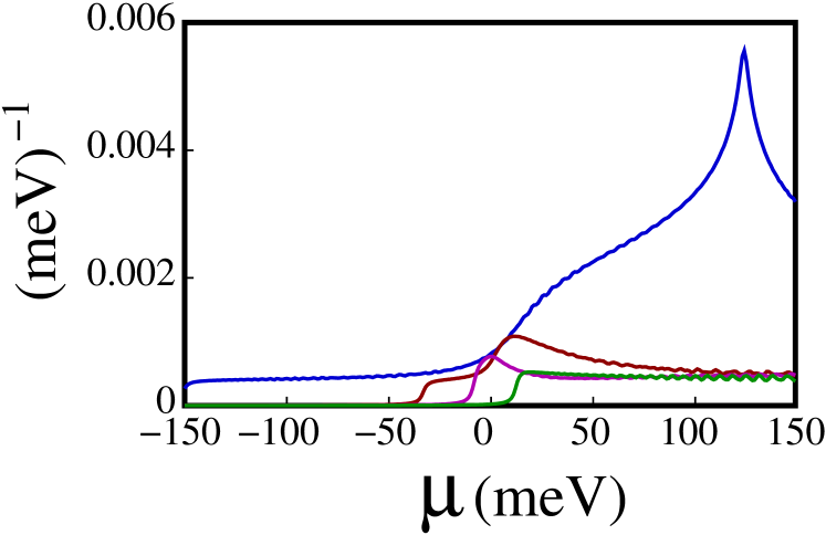
Figure 11: Contributions to the factor multiplying $N_{\rm Imp}\bar{u}^{2}$ at the right-hand side of Eq. (109) determined by setting $\tau_{\rm e}=3$ ps and averaged over band doublets, as a function of the chemical potential $\mu$. In order of increasing energy, the contributions are drawn in blue, red, magenta, and green.

In fact, looking at the right-hand side of Eq.(109), we see that, on varying $\mu$, terms with different index $\lambda$ contribute in a largely different way to the total sum. To evidence this, in Fig. 11 we plot (aside from the over-all factor $N_{\rm Imp}\bar{u}^{2}$) the contributions from the four different doublets, averaged over each doublet, as a function of $\mu$. As in Fig.8, it is useful to ideally split the plot in Fig. 11 into three regions. The first region approximatively corresponds to $-150\;{\rm mev}\leq\mu\leq-35\>{\rm meV}$. In this region we see that the contribution to the vertex correction just comes from the first doublet. This suggests us that the crude approximation resulting into Eq. (109) should not apply in this region: only two, out of eight, bands are contributing to $\tau_{\rm e}$ and, therefore, the average encoded in the right-hand side of the equations has to be performed over just 2, rather than $N=8$, bands. Consistently with this result, in computing the vertex correction we resort to a different approximation, by trading Eq. (109) for

$$1=\frac{N_{\rm Imp}\bar{u}^{2}}{2V}\sum_{\vec{k}}\sum_{\lambda=d_{xy;A}^{\pm}}\left[\frac{1}{\xi_{\vec{k},\lambda}^{2}+(2\tau_{\rm e})^{-2}}\right]\>\>\>\>,$$ (110)

with $d_{xy;A}^{\pm}$ denoting the $d_{xy;A}$ doublet. Having numerically set $\tau_{\rm e}$ as discussed above, Eq. (110) eventually trades for a numerical estimate of the (otherwise unknown) factor $N_{\rm Imp}\bar{u}^{2}$. To move ahead, leaving aside, for the time being, the second region, we now focus onto the third one, roughly ranging over the interval $50\;{\rm meV}\leq\mu\leq 150\;{\rm meV}$. While, in this region, the first doublet still provides by a large amount the leading contribution to the right-hand side of Eq. (109), there is, now, a finite contributions from the other three doublets, which is approximatively the same over the various subbands. This suggests to weight the contributions of all four the doublets by first separately assuming that the right-hand side of Eq. (109) is contributed by a single doublet only, for all four the doublets, and by then attributing to all the integrals a weight that is the same for the three higher-energy doublet and, obviously, higher for the lowest-energy one. This eventually results into an effective normalization factor at the right-hand side of Eq. (109), $N_{\rm Eff}$, such that $2<N_{\rm Eff}<8$, with $N_{\rm Eff}$ numerically determined as stated above. This allows us to estimate $N_{\rm Imp}\bar{u}^{2}$ throughout the third region, as well. Finally, a straightforward extension of the method we used for the third region to the second region, as well, with different weights for different doublets, in general, allows for estimating $N_{\rm Imp}\bar{u}^{2}$ throughout this region, as well.

We now proceed with computing the sheet- and the spin-Hall conductances. Let us begin with the sheet conductance.

Within the linear response theory of Appendix A, for a system in a Hall bar arrangement such as the one we draw in Fig. 1, the sheet conductance $\sigma_{s}$ is recovered from the current response along $x$ to an electric field applied in the same direction. Adding also the effects of the impurities we obtain, according to the result of Appendixes A and B, $\sigma_{s}=\sigma_{s;A}+\sigma_{s;B}$, with $\sigma_{s;A}$ accounting for the nonzero, impurity-induced imaginary part of the single-electron self-energy and $\sigma_{s;B}$ determined by vertex corrections.

From the derivation of Appendix B and taking into account our discussion above, we obtain

$$\sigma_{s;A} \approx \frac{1}{2\pi wV}\>\sum_{\vec{k}}\>\sum_{\lambda,\lambda^{\prime}}\>[j_{{\rm ch},x}]_{(\vec{k},\lambda);(\vec{k},\lambda^{\prime})}\>[j_{{\rm ch},x}]_{(\vec{k},\lambda^{\prime});(\vec{k},\lambda)}\times$$ (111)

$$\left\{\frac{(2\tau_{\rm e})^{-1}}{\xi_{\vec{k},\lambda}^{2}+(2\tau_{\rm e})^{-2}}\>\frac{(2\tau_{\rm e})^{-1}}{\xi_{\vec{k},\lambda^{\prime}}^{2}+(2\tau_{\rm e})^{-2}}\right\}\;\;\;\;,$$

with $w$ being the sample width along the $z$ direction, which we drop from our calculation, as we are only interested in the dependence of $\sigma_{s}$ on the chemical potential $\mu$. The electric current operator matrix elements $[j_{{\rm ch},x}]_{(\vec{k},\lambda);(\vec{k},\lambda^{\prime})}$ are derived by acting with the transformation in Eq. (5) over the operator $[j_{{\rm ch},x}]_{(\vec{k},\sigma);(\vec{k},\sigma^{\prime})}=e\left[\frac{\partial{\cal H}_{\rm 8-band}(\vec{k})}{\partial k_{x}}\right]_{\sigma,\sigma^{\prime}}=e\left[v^{x}\right]_{\sigma,\sigma^{\prime}}$.

Along the same guidelines leading to Eq. (111), we derive the contribution to the sheet conductance arising from the vertex corrections, $\sigma_{s;B}$. This is given by

$$\sigma_{s;B} = \frac{e^{2}}{2\pi wV}\>\sum_{\vec{k}}\>\sum_{\lambda,\lambda^{\prime}}\>[v^{x}]_{(\vec{k},\lambda);(\vec{k},\lambda^{\prime})}\>[\delta v^{x}]_{(\vec{k},\lambda^{\prime});(\vec{k},\lambda)}\times$$ (112)

$$\left\{\frac{1}{\xi_{\vec{k},\lambda}+i(2\tau_{\rm e})^{-1}}\>\frac{1}{\xi_{\vec{k},\lambda^{\prime}}-i(2\tau_{\rm e})^{-1}}\right\}\;\;\;\;.$$

The quantity $\delta v^{x}$ in Eq.(112) is the correction to the interaction vertex $[v^{x}]_{(\vec{k},\lambda);(\vec{k}^{\prime},\lambda^{\prime})}$, which we numerically compute through an iterative process in the impurity interaction strength, as we outline in Appendix B. Doing so, we explicitly verified that $\sigma_{s;B}$, is several orders of magnitude lower than the contribution $\sigma_{s;A}$ in Eq. (111). We therefore used only this last contribution to estimate $\sigma_{s}$ and to accordingly draw the plot in Fig. 4.

To compute the spin-Hall conductance $\sigma_{xy}^{z}$ we proceed in the same way. First of all, we split again $\sigma_{xy}^{z}$ as $\sigma_{xy}^{z}=\sigma_{xy;A}^{z}+\sigma_{xy;B}^{z}$, with $\sigma_{xy;A}^{z}$ taking into account the finite self-energy of the single-particle Green’s functions and $\sigma_{xy;B}^{z}$ accounting for the impurity-induced vertex corrections. To perform our derivation, we need the retarded Green’s functions of the operators $j_{{\rm sp},x}^{z}=\frac{1}{2}\{\frac{\partial{\cal H}_{\rm 8-band}(\vec{k})}{\partial k_{x}},{\bf I}\otimes\sigma_{z}\}$ and $j_{{\rm ch},y}=e\frac{\partial{\cal H}_{\rm 8-band}(\vec{k})}{\partial k_{y}}$. By direct inspection we verified that $\Re e\{[j_{{\rm sp},x}^{z}]_{(\vec{k},\lambda);(\vec{k},\lambda^{\prime})}[j_{{\rm ch},y}]_{(\vec{k},\lambda^{\prime});(\vec{k},\lambda)}\}=0$. Therefore, $\sigma_{xy;A}^{z}$ is only contributed by the term in Eq.(29), while the contribution from Eq.(28) is equal to 0. Specifically, we obtain

$$\sigma_{xy;A}^{z}=-\frac{i}{2V}\>\sum_{\vec{k}}\>\sum_{\lambda,\lambda^{{}^{\prime}}}\times$$

$$\Im m\{[j_{{\rm sp},x}^{z}]_{(\vec{k},\lambda);(\vec{k},\lambda^{\prime})}[j_{{\rm ch},y}]_{(\vec{k},\lambda^{\prime});(\vec{k},\lambda)}\}\times$$

$$\int\frac{d\bar{\omega}}{2\pi}\>\Biggl{\{}[g_{(\vec{k},\lambda)}^{A}(\bar{\omega})-g_{(\vec{k},\lambda)}^{R}(\bar{\omega})]\times$$

$$\partial_{\bar{\omega}}[g_{(\vec{k},\lambda^{\prime})}^{A}(\bar{\omega})+g_{(\vec{k},\lambda^{\prime})}^{R}(\bar{\omega}))]f(\bar{\omega})\Biggr{\}}\>,$$

(113)

with (see Appendix A for details)

$$g_{(\vec{k},\lambda)}^{R/A}(\bar{\omega})=\frac{1}{\bar{\omega}-\xi_{\vec{k},\lambda}\pm\frac{i}{2\tau_{\rm e}}}\>\>\>\>,$$ (114)

and $f(\bar{\omega})$ being the Fermi distribution function.

The contribution from vertex corrections, $\sigma_{xy;B}^{z}$, takes a form similar to $\sigma_{s;B}$ in Eq. (112), provided the operators entering the corresponding equation are pertinently replaced. As a result, we obtain

$$\sigma_{xy;B}^{z} = \frac{1}{2\pi V}\>\sum_{\vec{k}}\>\sum_{\lambda,\lambda^{\prime}}[\delta j_{{\rm sp},x}^{z}]_{(\vec{k},\lambda);(\vec{k},\lambda^{\prime})}\>[j_{{\rm ch},y}]_{(\vec{k},\lambda^{\prime});(\vec{k},\lambda)}\times$$ (115)

$$\left\{\frac{1}{\xi_{\vec{k},\lambda}+i(2\tau_{\rm e})^{-1}}\>\frac{1}{\xi_{\vec{k},\lambda^{\prime}}-i(2\tau_{\rm e})^{-1}}\right\}\;\;\;\;,$$

with the vertex correction $\delta j_{{\rm sp},x}^{z}$ computed according to Eqs. (51)-(53) and the self-consistent expression for $\tau_{\rm e}$ implemented as discussed above.

Eqsations (111) and (112) and (113) and (114) provide the expressions we used in the main text to draw the plots of the sheet conductance and of the spin-Hall conductance, in the clean limit, as well as in the presence of impurities.

Before concluding this appendix, we briefly investigate how changing the density of impurities and/or the impurity interaction potential affects $\sigma_{s}$ and $\sigma_{xy}^{z}$. To do so, it is worth pointing out that, throughout our derivation, we lump all the details about the density of impurity and the impurity interaction into the parameter $\tau_{\rm Imp}$, which we regard as a phenomenological parameter, fitted from the data of Ref.Trier et al. (2020). Therefore, we analyze the effects of changing the density of impurities and/or the impurity interaction potential by simply computing the conductances as functions of $\mu$ for different values of $\tau_{\rm Imp}$. In Fig. 12(a) we plot the corresponding results for $\sigma_{s}$ as a function of $\mu$ computed using the parameters listed in Table 1, for $\tau_{\rm Imp}=3,\>6$ and 9 ps. As expected, at a given $\mu$, $\sigma_{s}$ increases monotonically, as a function of $\tau_{\rm Imp}$, with no particular additional features in the main behavior (for $\tau_{\rm Imp}=6$ and 9 ps), compared to the case $\tau_{\rm Imp}=3$ ps, corresponding to the value estimated from the data of Ref. Trier et al. (2020). In Fig. 12(b) we plot $\sigma_{xy;A}^{z}$ as a function of $\mu$ for the same values of $\tau_{\rm Imp}$ as we used for $\sigma_{s}$ and, in addition, for $\tau_{\rm Imp}^{-1}=0$. The over-all main trend shows how, varying $\tau_{\rm Imp}$, the plot in the clean limit evolves into the one at finite $\tau_{\rm Imp}$, with no particular features emerging at values in between $\tau_{\rm Imp}^{-1}=0$ (the clean limit) and the experimentally estimated value $\tau_{\rm Imp}=3\>{\rm ps}$.

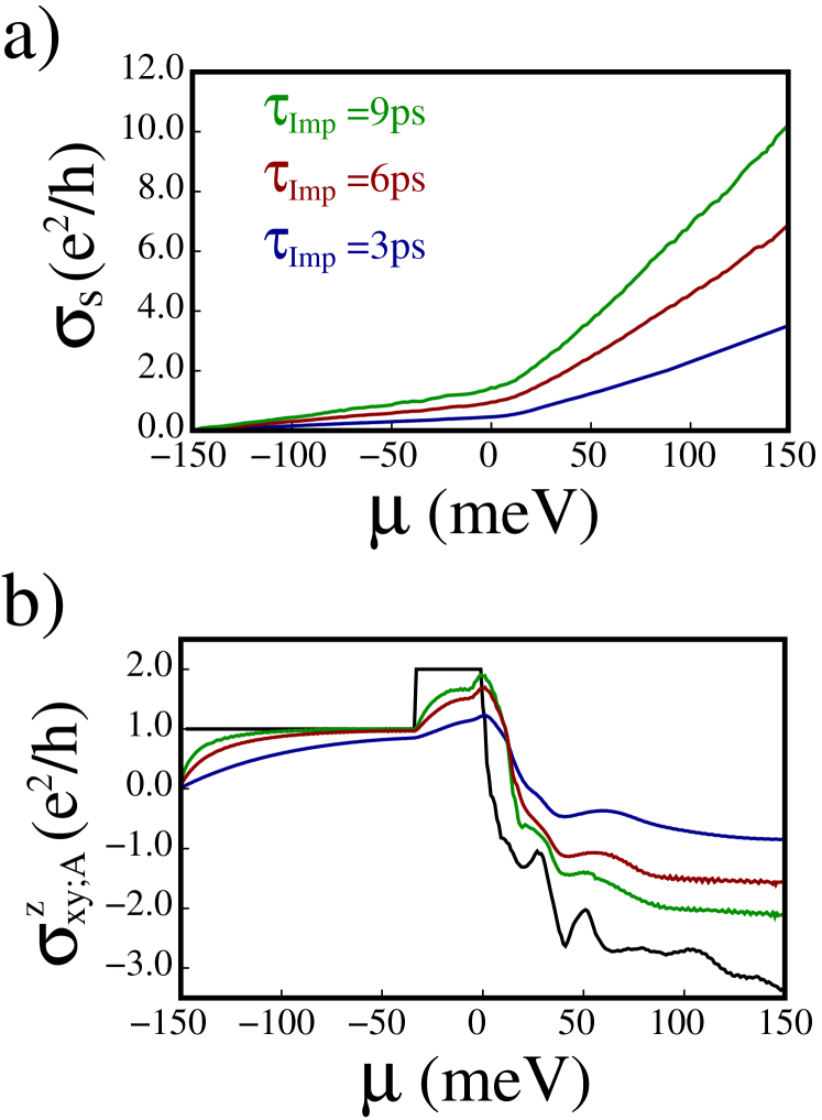
Figure 12: (a): $\sigma_{s}$ as a function of $\mu$ computed with the parameters listed in Table 1, and with $\tau_{\rm Imp}=3\>{\rm ps}$, $\tau_{\rm Imp}=6\>{\rm ps}$ (red curve), and $\tau_{\rm Imp}=9\>{\rm ps}$ (green curve). (b):$\sigma_{xy;A}^{z}$ as a function of $\mu$ computed with the parameters listed in Table 1, and with $\tau_{\rm Imp}^{-1}=0$ (black curve), $\tau_{\rm Imp}=3\>{\rm ps}$, $\tau_{\rm Imp}=6\;{\rm ps}$ (red curve), and $\tau_{\rm Imp}=9\;{\rm ps}$ (green curve).

References

- Wolf et al. (2001) S. A. Wolf, D. D. Awschalom, R. A. Buhrman, J. M. Daughton, S. von Molnár, M. L. Roukes, A. Y. Chtchelkanova, and D. M. Treger, Science 294, 1488 (2001).
- Vaz et al. (2019) D. C. Vaz, P. Noël, A. Johansson, B. Göbel, F. Y. Bruno, G. Singh, S. McKeown-Walker, F. Trier, L. M. Vicente-Arche, A. Sander, S. Valencia, P. Bruneel, M. Vivek, M. Gabay, N. Bergeal, F. Baumberger, H. Okuno, A. Barthélémy, A. Fert, L. Vila, I. Mertig, J.-P. Attané, and M. Bibes, Nature Materials 18, 1187 (2019).
- Hirohata et al. (2020) A. Hirohata, K. Yamada, Y. Nakatani, I.-L. Prejbeanu, B. Diény, P. Pirro, and B. Hillebrands, Journal of Magnetism and Magnetic Materials 509, 166711 (2020).
- Chauleau et al. (2016) J.-Y. Chauleau, M. Boselli, S. Gariglio, R. Weil, G. de Loubens, J.-M. Triscone, and M. Viret, Europhysics Letters 116, 17006 (2016).
- Song et al. (2017) Q. Song, H. Zhang, T. Su, W. Yuan, Y. Chen, W. Xing, J. Shi, J. Sun, and W. Han, Science Advances 3, e1602312 (2017), https://www.science.org/doi/pdf/10.1126/sciadv.1602312 .
- Telesio et al. (2018) F. Telesio, R. Moroni, I. Pallecchi, D. Marré, G. Vinai, G. Panaccione, P. Torelli, S. Rusponi, C. Piamonteze, E. di Gennaro, A. Khare, F. M. Granozio, and A. Filippetti, Journal of Physics Communications 2, 025010 (2018).
- Edelstein (1990) V. Edelstein, Solid State Communications 73, 233 (1990).
- Dyakonov and Perel (1971) M. Dyakonov and V. Perel, Physics Letters A 35, 459 (1971).
- Sinova et al. (2015) J. Sinova, S. O. Valenzuela, J. Wunderlich, C. H. Back, and T. Jungwirth, Rev. Mod. Phys. 87, 1213 (2015).
- Qian et al. (2014) X. Qian, J. Liu, L. Fu, and J. Li, Science 346, 1344 (2014), https://www.science.org/doi/pdf/10.1126/science.1256815 .
- Nie et al. (2015) S. M. Nie, Z. Song, H. Weng, and Z. Fang, Phys. Rev. B 91, 235434 (2015).
- Safeer et al. (2019) C. K. Safeer, J. Ingla-Aynés, F. Herling, J. H. Garcia, M. Vila, N. Ontoso, M. R. Calvo, S. Roche, L. E. Hueso, and F. Casanova, Nano Letters 19, 1074 (2019).
- Benítez et al. (2020) L. A. Benítez, W. Savero Torres, J. F. Sierra, M. Timmermans, J. H. Garcia, S. Roche, M. V. Costache, and S. O. Valenzuela, Nature Materials 19, 170 (2020).
- Safeer et al. (2020) C. K. Safeer, J. Ingla-Aynés, N. Ontoso, F. Herling, W. Yan, L. E. Hueso, and F. Casanova, Nano Letters 20, 4573 (2020).
- Farzaneh and Rakheja (2020) S. M. Farzaneh and S. Rakheja, Phys. Rev. Mater. 4, 114202 (2020).
- Trier et al. (2020) F. Trier, D. C. Vaz, P. Bruneel, P. Noël, A. Fert, L. Vila, J.-P. Attané, A. Barthélémy, M. Gabay, H. Jaffrès, and M. Bibes, Nano Letters 20, 395 (2020), pMID: 31859513.
- Sinova et al. (2004) J. Sinova, D. Culcer, Q. Niu, N. A. Sinitsyn, T. Jungwirth, and A. H. MacDonald, Phys. Rev. Lett. 92, 126603 (2004).
- King et al. (2014) P. D. C. King, S. McKeown Walker, A. Tamai, A. de la Torre, T. Eknapakul, P. Buaphet, S. K. Mo, W. Meevasana, M. S. Bahramy, and F. Baumberger, Nature Communications 5, 3414 (2014).
- Ohtomo and Hwang (2004) A. Ohtomo and H. Y. Hwang, Nature 427, 423 (2004).
- Chen et al. (2011) Y. Chen, N. Pryds, J. E. Kleibeuker, G. Koster, J. Sun, E. Stamate, B. Shen, G. Rijnders, and S. Linderoth, Nano Letters 11, 3774 (2011).
- Rödel et al. (2016) T. C. Rödel, F. Fortuna, S. Sengupta, E. Frantzeskakis, P. L. Fèvre, F. Bertran, B. Mercey, S. Matzen, G. Agnus, T. Maroutian, P. Lecoeur, and A. F. Santander-Syro, Advanced Materials 28, 1976 (2016).
- Caviglia et al. (2008) A. D. Caviglia, S. Gariglio, N. Reyren, D. Jaccard, T. Schneider, M. Gabay, S. Thiel, G. Hammerl, J. Mannhart, and J. M. Triscone, Nature 456, 624 (2008).
- Caviglia et al. (2010) A. D. Caviglia, M. Gabay, S. Gariglio, N. Reyren, C. Cancellieri, and J.-M. Triscone, Phys. Rev. Lett. 104, 126803 (2010).
- Trama et al. (2021) M. Trama, V. Cataudella, and C. A. Perroni, Phys. Rev. Research 3, 043038 (2021).
- Lesne et al. (2016) E. Lesne, Y. Fu, S. Oyarzun, J. C. Rojas-Sànchez, D. C. Vaz, H. Naganuma, G. Sicoli, J. P. Attané, M. Jamet, E. Jacquet, J. M. George, A. Barthélémy, H. Jaffrès, A. Fert, M. Bibes, and L. Vila, Nature Materials 15, 1261 (2016).
- Varignon et al. (2018) J. Varignon, L. Vila, A. Barthélémy, and M. Bibes, Nature Physics 14, 322 (2018).
- Abanin et al. (2009) D. A. Abanin, A. V. Shytov, L. S. Levitov, and B. I. Halperin, Phys. Rev. B 79, 035304 (2009).
- Mishchenko et al. (2004) E. G. Mishchenko, A. V. Shytov, and B. I. Halperin, Phys. Rev. Lett. 93, 226602 (2004).
- Inoue et al. (2004) J.-i. Inoue, G. E. W. Bauer, and L. W. Molenkamp, Phys. Rev. B 70, 041303 (2004).
- Khaetskii (2006) A. Khaetskii, Phys. Rev. Lett. 96, 056602 (2006).
- Raimondi and Schwab (2005) R. Raimondi and P. Schwab, Phys. Rev. B 71, 033311 (2005).
- Dimitrova (2005) O. V. Dimitrova, Phys. Rev. B 71, 245327 (2005).
- Perroni et al. (2019) C. A. Perroni, V. Cataudella, M. Salluzzo, M. Cuoco, and R. Citro, Phys. Rev. B 100, 094526 (2019).
- Bistritzer et al. (2011) R. Bistritzer, G. Khalsa, and A. H. MacDonald, Phys. Rev. B 83, 115114 (2011).
- Michaeli et al. (2012) K. Michaeli, A. C. Potter, and P. A. Lee, Phys. Rev. Lett. 108, 117003 (2012).
- Khalsa et al. (2013) G. Khalsa, B. Lee, and A. H. MacDonald, Phys. Rev. B 88, 041302 (2013).
- Shanavas et al. (2014) K. V. Shanavas, Z. S. Popović, and S. Satpathy, Phys. Rev. B 90, 165108 (2014).
- Borge et al. (2014) J. Borge, C. Gorini, G. Vignale, and R. Raimondi, Phys. Rev. B 89, 245443 (2014).
- Rashba (2004) E. I. Rashba, Phys. Rev. B 70, 201309 (2004).
- Shytov et al. (2006) A. V. Shytov, E. G. Mishchenko, H.-A. Engel, and B. I. Halperin, Phys. Rev. B 73, 075316 (2006).
- Vivek et al. (2017) M. Vivek, M. O. Goerbig, and M. Gabay, Phys. Rev. B 95, 165117 (2017).
- Huijben et al. (2017) M. Huijben, G. W. J. Hassink, M. P. Stehno, Z. L. Liao, G. Rijnders, A. Brinkman, and G. Koster, Phys. Rev. B 96, 075310 (2017).
- Joshua et al. (2012) A. Joshua, S. Pecker, J. Ruhman, E. Altman, and S. Ilani, Nature Communications 3, 1 (2012).
- Johansson et al. (2021) A. Johansson, B. Göbel, J. Henk, M. Bibes, and I. Mertig, Phys. Rev. Research 3, 013275 (2021).
- Nachawaty et al. (2018) A. Nachawaty, M. Yang, S. Nanot, D. Kazazis, R. Yakimova, W. Escoffier, and B. Jouault, Phys. Rev. B 98, 045403 (2018).
- Tagliacozzo et al. (2019) A. Tagliacozzo, G. Campagnano, D. Giuliano, P. Lucignano, and B. Jouault, Phys. Rev. B 99, 155417 (2019).
- Diez et al. (2015) M. Diez, A. Monteiro, G. Mattoni, E. Cobanera, T. Hyart, E. Mulazimoglu, N. Bovenzi, C. Beenakker, and A. Caviglia, Phys. Rev. Lett. 115, 016803 (2015).
- Trama et al. (2022) M. Trama, V. Cataudella, C. A. Perroni, F. Romeo, and R. Citro, Nanomaterials 12, 2494 (2022).
- Trier et al. (2022) F. Trier, P. Noël, J.-V. Kim, J.-P. Attané, L. Vila, and M. Bibes, Nature Reviews Materials 7, 258 (2022).
- Schwab and Raimondi (2002) P. Schwab and R. Raimondi, The European Physical Journal B - Condensed Matter and Complex Systems 25, 483 (2002).
- Kane and Mele (2005) C. L. Kane and E. J. Mele, Phys. Rev. Lett. 95, 146802 (2005).
- Lepori et al. (2021) L. Lepori, D. Giuliano, A. Nava, and C. A. Perroni, Phys. Rev. B 104, 134509 (2021).