Quick Adaptive Ternary Segmentation: An Efficient Decoding Procedure For Hidden Markov Models

Abstract

Hidden Markov models (HMMs) are characterized by an unobservable (hidden) Markov chain and an observable process, which is a noisy version of the hidden chain. Decoding the original signal (i.e., hidden chain) from the noisy observations is one of the main goals in nearly all HMM based data analyses. Existing decoding algorithms such as the Viterbi algorithm have computational complexity at best linear in the length of the observed sequence, and sub-quadratic in the size of the state space of the Markov chain.

We present Quick Adaptive Ternary Segmentation (QATS), a divide-and-conquer procedure which decodes the hidden sequence in polylogarithmic computational complexity in the length of the sequence, and cubic in the size of the state space, hence particularly suited for large scale HMMs with relatively few states. The procedure also suggests an effective way of data storage as specific cumulative sums. In essence, the estimated sequence of states sequentially maximizes local likelihood scores among all local paths with at most three segments. The maximization is performed only approximately using an adaptive search procedure. The resulting sequence is admissible in the sense that all transitions occur with positive probability.

To complement formal results justifying our approach, we present Monte–Carlo simulations which demonstrate the speedups provided by QATS in comparison to Viterbi, along with a precision analysis of the returned sequences. An implementation of QATS in C++ is provided in the R-package QATS and is available from GitHub.

Keywords:

Hidden Markov model, Local search, Massive data, Polylogarithmic runtime, Segmentation

AMS 2000 subject classification:

62M05

1 Introduction

A hidden Markov model (HMM), $(\boldsymbol{X},\boldsymbol{Y})=(X_{k},Y_{k})_{k\geq 1}$, defined on a probability space $(\Omega,{\cal F},\mathop{\rm I\!P}\nolimits)$, consists of an unobservable (hidden) homogeneous Markov chain $\boldsymbol{X}$ with finite state space ${\cal X}=\{1,2,\ldots,m\}$, $m\geq 2$, and an observable stochastic process $\boldsymbol{Y}$ that takes values in a measurable space $({\cal Y},{\cal B})$. Conditionally on $\boldsymbol{X}$, the process $\boldsymbol{Y}$ is stochastically independent, and each $Y_{k}$ depends on $\boldsymbol{X}$ only through $X_{k}$.

Because of the generality of the observation and state spaces, HMMs are sufficiently generic to capture the complexity of various real-world time series, and meanwhile the simple Markovian dependence structure allows efficient computations. Upon more than half a century of development, HMMs and variants thereof have been established as one of the most successful statistical modeling ideas, see for example Ephraim and Merhav (2002), Cappé et al. (2005) and Mor et al. (2021) for an overview. Since their early days, they are widely used in various fields of science and applications, such as speech recognition (Rabiner, 1989; Gales and Young, 2008), DNA or protein sequencing (Durbin et al., 1998; Karplus, 2009), ion channel modeling (Ball and Rice, 1992; Pein et al., 2021) and fluctuation characterization in macro economic time series (Hamilton, 1989; Frühwirth-Schnatter, 2006), to name only a few.

Increasingly large and complex datasets with long time series have recently led to a revival in the development of scalable algorithms and methodologies for HMMs, see Bulla et al. (2019) and the related literature in Sections 1.1 and 1.2. In the present paper, we focus on computational aspects involved in the estimation of the hidden state sequence for large scale HMMs, that is when $n\gg m$. Here, $n$ denotes the length of the sequence of observations $\boldsymbol{y}=\boldsymbol{y}_{1:n}:=(y_{k})_{k=1}^{n}$ from $\boldsymbol{Y}_{1:n}:=(Y_{k})_{k=1}^{n}$. The goal is, as Rabiner (1989) formulated it, to “find the ‘correct’ state sequence” behind $\boldsymbol{y}$. Procedures achieving such a task are commonly known as segmentation or decoding methods, and existing segmentation methods are tailored to what is exactly meant by the ‘correct’ state sequence.

To simplify, we assume that the parameters of the HMM are (approximately) known. These parameters are the transition matrix $\boldsymbol{p}:=(p_{ij})_{i,j\in{\cal X}}$ of the Markov chain $\boldsymbol{X}$ with $p_{ij}=\mathop{\rm I\!P}\nolimits(X_{k+1}=j|X_{k}=i)$, the initial probability vector $\boldsymbol{\pi}:=(\pi_{i})_{i\in{\cal X}}$ with $\pi_{i}=\mathop{\rm I\!P}\nolimits(X_{1}=i)$, and the distribution of $Y_{k}$ given $X_{k}=i$ which we assume to have density $f_{i}$ with respect to some dominating measure $\mu$ on ${\cal B}$. If the parameters are unknown, they are typically estimated via maximum likelihood or EM algorithms (Baum and Petrie, 1966; Baum et al., 1970; Baum, 1972). As we have large scale data scnearios in mind, this is not a severe burden as it can be sped-up for instance by using a fraction of the complete data (Gotoh et al., 1998) while keeping statistical precision accurate.

For natural numbers $1\leq\ell\leq r$ and an arbitrary vector $\boldsymbol{\xi}$ of dimension at least $r$, we write $\ell{:}r$ for an index interval $\{\ell,\ell+1,\ldots,r\}$, and call it a segment, and write $\boldsymbol{\xi}_{\ell:r}$ for the vector $(\xi_{k})_{k=\ell}^{r}$. We also call segments of a vector $\boldsymbol{\xi}$ the maximal index intervals on which $\boldsymbol{\xi}$ is constant, i.e. the segment $\ell{:}r$ is a segment of $\boldsymbol{\xi}$ if there exists $\xi$ such that $\xi_{k}=\xi$ for all $k\in\ell{:}r$, $\xi_{\ell-1}\neq\xi_{\ell}$ and $\xi_{r}\neq\xi_{r+1}$. We interpret all vectors as row-vectors.

1.1 Maximum a posteriori — Viterbi path

The most common segmentation method aims to find the most likely state sequence $\boldsymbol{x}$ given the observations $\boldsymbol{y}$. Formally, it seeks a path $\boldsymbol{x}\in{\cal X}^{n}$ which is a mode of the complete likelihood

$$\Lambda_{1:n}(\boldsymbol{x})\ :=\ \pi_{x_{1}}f_{x_{1}}(y_{1})\left(\prod_{k=2}^{n}p_{x_{k-1},x_{k}}f_{x_{k}}(y_{k})\right).$$ (1.1)

Such a sequence is commonly known as maximum a posteriori (MAP) or Viterbi path, named after the algorithm of Viterbi (1967) which determines such a path via dynamic programming, see Forney (1973), for more details. In its most common implementation, the Viterbi algorithm, simply referred to as Viterbi in the sequel, has computational complexity ${\cal O}(m^{2}n)$, see also Algorithm 6.

Due to the ever increasing size and complexity of datasets, there is interest in accelerating Viterbi (Bulla et al., 2019). Several authors obtained sub-quadratic complexity in the size $m$ of the state space. For instance, Esposito and Radicioni (2009) modified Viterbi and achieved a best-case complexity of ${\cal O}(m\log(m)n)$. At each step of the dynamic program, their approach avoids inspecting all potential states by ranking them and stopping the search as soon as a certain state is too unlikely. Kaji et al. (2010) later proposed to reduce the number of states examined by Viterbi by creating groups of states at each step of the dynamic program and iteratively modifying those groups, when necessary. In the best case, the complexity of their method is ${\cal O}(n)$. Both Esposito and Radicioni (2009) and Kaji et al. (2010) have worst-case complexity equal to that of Viterbi. In contrast, Cairo et al. (2016) were the first to propose an algorithm with worst-case complexity ${\cal O}((m^{2}/\log m)n)$ (and an extra prepossessing cost that is polynomial in $m$ and $n$) by improving the matrix-vector multiplication performed at each step of the dynamic program. All those methods find a maximizer of (1.1). Note that improving Viterbi by a polynomial factor in $m$, or more, would have important implications in fundamental graph problems, as argued in Backurs and Tzamos (2017).

There have been attempts at decreasing the computational complexity of Viterbi in the length $n$ of the observed sequence $\boldsymbol{y}$. Lifshits et al. (2009) used compression and considered the setting of an observation space with finite support, that is, ${\cal Y}$ has finite cardinality. They proposed to precompress $\boldsymbol{y}$ by exploiting repetitions in that sequence, and achieved varying speedups (e.g. by a factor $\Theta(\log n)$) depending on the compression scheme used. Hassan et al. (2021) presented a framework for HMMs which allows to apply the parallel-scan algorithm (Ladner and Fischer, 1980; Blelloch, 1989) and yields a parallel computation of the forward and backward loops of Viterbi. This parallel framework can achieve a span complexity of ${\cal O}(m^{2}\log n)$, but it necessitates a number of threads that is proportional to $n/\log(n)$ and results in a total complexity of ${\cal O}(m^{2}n)$.

1.2 Other risk-based segmentation methods

Maximizing the complete likelihood as executed by Viterbi may share common disadvantages with other MAP estimators, see Carvalho and Lawrence (2008). For instance, Viterbi may perform unsatisfactorily if there are several concurring paths with similar probabilities. A different optimality criterion determines, at each time $k\in 1{:}n$, the most likely state $\widehat{x}_{k}$ which gave rise to observation $y_{k}$, given the whole sequence $\boldsymbol{y}$. The solution to this problem minimizes the expected number of misclassifications and is known as the pointwise maximum a posteriori (PMAP) estimator, which is often referred to as posterior decoding in bioinformatics and computational biology (Durbin et al., 1998). To obtain the PMAP, a forward-backward algorithm similar to Viterbi computes the so-called smoothing and filtering distributions, which give the distribution of $X_{k}$ given $\boldsymbol{Y}_{1:n}$ and $X_{k}$ given $\boldsymbol{Y}_{1:k}$, $k\in 1{:}n$, respectively, see Baum et al. (1970) and Rabiner (1989). The PMAP also has computational complexity ${\cal O}(m^{2}n)$. There is an important drawback of the PMAP paradigm for estimation: The resulting sequence $\widehat{\boldsymbol{x}}$ is potentially inadmissible, that is, it can happen that $p_{\widehat{x}_{k},\widehat{x}_{k+1}}=0$ for some $1\leq k<n$, that is, the probability to transition from $\widehat{x}_{k}$ to $\widehat{x}_{k+1}$ is zero.

Lember and Koloydenko (2014) studied the MAP and PMAP within a risk-based framework, where these two estimators are seen as minimizers of specific risks. By mixing those risks and other relevant ones, hybrid estimators combining desirable properties of both estimators are defined, see also Fariselli et al. (2005). Also in this case, suitable modifications of the forward-backward algorithm are possible to maintain a computational complexity of ${\cal O}(m^{2}n)$.

Provided that there is a priori knowledge about the number of segments of the hidden path, Titsias et al. (2016) determined a most likely path with a user-specified number $s$ of segments (sMAP). Precisely, they attempt to maximize $\Lambda_{1:n}(\boldsymbol{x})$ over all paths $\boldsymbol{x}\in{\cal X}^{n}$ such that the cardinality of $\{k:x_{k}\neq x_{k+1}\}$ is equal to $s-1$. The complexity of their method is ${\cal O}(sm^{2}n)$, and if one desires to look at all paths with up to $s_{\max}$ segments, the overall complexity amounts to ${\cal O}(s_{\max}m^{2}n)$.

1.3 Our contribution

We present a novel decoding procedure inspired by Viterbi and sMAP, and which achieves polylogarithmic computational complexity in terms of the sample size $n$. Our method is particularly beneficial for HMMs with relatively infrequent changes of hidden states, since the case of frequent changes approaches a linear computational complexity, let alone to output the changes of state. The segmentation of HMMs with infrequent changes can be viewed as a particular problem of (sparse) change point detection, see recent surveys by Niu et al. (2016) and Truong et al. (2020).

Considering the problem from this point of view, we introduce Quick Adaptive Ternary Segmentation (QATS), a fast segmentation method for HMMs. In brief, QATS sequentially partitions the index interval $1{:}n$ into smaller segments with the following property: On each given segment, the state sequence that maximizes a localized version of the complete likelihood (1.1), over all state sequences with at most three segments (at most two changes of state), is in fact a constant state sequence (it has a single segment, that is no change of state). That means, if at a certain stage of the procedure the maximizing sequence is made of two or three segments (one or two changes of state), then those two or three segments replace the original segment in the partition and those new segments are subsequently investigated for further partitioning.

This divide-and-conquer technique builds on the classical binary segmentation (Bai, 1997) where at most one split at a time can be created. Here, we allow up to two splits per iteration (three new segments), granting it the name of ternary segmentation. The benefit of considering three segments instead of two is the significant increase in detection power of change points, see 3.3 for a theoretical justification. In principle, one could consider more than three segments for the sake of further improvement in detection power, but this would come at the cost of a heavier computational burden. A variant of ternary segmentation that searches for a bump in a time series was first considered in Levin and Kline (1985), the idea of which can also be found in circular binary segmentation (Olshen et al., 2004). However, the concept of optimizing over two sample locations is much older and can already be found in the proposal by Page (1955).

To the best of our knowledge, binary or ternary segmentation, or any extension thereof, has not yet been used for decoding HMMs so far. A possible reason is that the resulting path, which we call QATS-path, does not maximize an explicit score defined a priori, unlike the MAP, PMAP or sMAP discussed previously. Instead, the QATS-path solves a problem defined implicitly via recursive local maximizations. We provide a mathematical justification for QATS, and our simulation study shows that QATS estimates the true hidden sequence with a precision comparable to that of its competitors, while being substantially faster already for moderate sized datasets. More precisely, if $s$ denotes the number of segments of the QATS-path, we prove that QATS has computational complexity ${\cal O}(sm^{3}\log n)$. In case of a small number $m$ of states and a large number $n$ of observations, this can be significantly faster than the computational complexity ${\cal O}\bigl{(}m^{2}n/\log(\max\{m,n\})\bigr{)}$ of the state-of-the-art accelerations of Viterbi, see Section 1.1.

In order to achieve this important speedup, the maximization step at each iteration of the ternary segmentation is only performed approximately, in the sense that the best path with at most three segments may not be obtained, but a sufficiently good one will be found quickly. To rapidly obtain this path, we devise an adaptive search strategy inspired by the optimistic search algorithm of Kovács et al. (2020) in the context of change point detection. The original idea of adaptive searches can be traced back to golden section search (Kiefer, 1953). The application of such an adaptive search is possible here because data are stored as cumulative sums of log-densities evaluated at the observations $\boldsymbol{y}$.

The reasons why the surprising speed-up from ${\cal O}(n)$ to ${\cal O}(\log n)$ with little loss of statistical performance is possible at all can be summarized as follows:

1. The switch of optimization perspectives. We look for the sample locations at which the hidden states most likely change among all sample locations, instead of finding the most likely hidden state for every sample location, like Viterbi.

2. The search of three segments in each step. The choice of three segments (rather than two) is empirically shown to provide a successful balance in the trade-off between computational efficiency and statistical performance.

3. The estimation of changes via local optima. We demonstrate that the locations at which the hidden states change can be characterized through the likelihood score by local optima, which can be estimated much faster than a global one. It is exactly the search for a local optimum rather than the global one that makes a fast algorithm requiring only ${\cal O}(\log n)$ evaluations of likelihood scores possible.

4. The use of a local likelihood score. The local likelihood score has the benefit of being computable in ${\cal O}(1)$ operations since it consists in differences of certain partial sums under proper transformation.

The procedures devised in this article are collected in the R-package QATS and are available from https://github.com/AlexandreMoesching/QATS. All methods are also implemented in C++ using the linear algebra library Armadillo (Sanderson and Curtin, 2016, 2018) and made accessible to R (R Core Team, 2022) using Rcpp (Eddelbuettel and François, 2011; Eddelbuettel, 2013; Eddelbuettel and Balamuta, 2018) and RcppArmadillo (Eddelbuettel and Sanderson, 2014).

1.4 Structure of the paper

The rest of the article is organized as follows. In Section 2, we devise the QATS procedure formally. We provide computational guarantees and a computational complexity analysis of QATS. The theoretical results on QATS, including methodological justifications, sensitivity analysis, and path properties are collected in Section 3. In Section 4, we examine the empirical performance of QATS in terms of estimation accuracy and computational efficiency. Proofs and technical details are deferred to Appendix A.

2 Description of the procedure

The idea of QATS is to sequentially partition, or segment, the index interval $1{:}n$ into $s\geq 1$ contiguous and sorted segments $S_{1},S_{2},\ldots,S_{s}$, that is $S_{u}=\ell_{u}{:}r_{u}$ with indices $\ell_{u}\leq r_{u}$, $u\in 1{:}s$, such that $\ell_{1}=1$, $r_{s}=n$ and $r_{u}+1=\ell_{u+1}$, $u\in 1{:}(s-1)$. The segmentation achieves the following goal: On each segment $S_{u}$, the best local path with at most three segments is a constant path, i.e. it is made of only one segment.

Precisely, a path with $c\geq 1$ segments is a vector $\boldsymbol{x}\in{\cal X}^{d}$ with $c-1$ breaks, or change points: If $c>1$, there exists $\kappa_{0}:=1<\kappa_{1}<\cdots<\kappa_{c-1}<\kappa_{c}:=d+1$ such that $\boldsymbol{x}_{\kappa_{u-1}{:}(\kappa_{u}-1)}$ is a constant vector and $x_{\kappa_{u-1}}\neq x_{\kappa_{u}}$, for $u\in 1{:}c$. A constant path is thus the one that satisfies $\#\{x_{k}:k\in 1{:}d\}=c=1$, i.e. it is made of a single segment. Furthermore, on a given segment $S=\ell{:}r$, we define the local likelihood of $\boldsymbol{x}\in{\cal X}^{r-\ell+1}$ and $\boldsymbol{y}_{\ell{:}r}$, given a previous state $X_{\ell-1}=x_{0}\in{\cal X}$, as the following quantity (recall (1.1)):

$$\Lambda_{\ell:r}(\boldsymbol{x}|x_{0})\ :=\ \begin{cases}\Lambda_{1:r}(\boldsymbol{x})&\text{if}\ \ell=1,\\ \prod_{k=\ell}^{r}p_{x_{k-\ell},x_{k-\ell+1}}f_{x_{k-\ell+1}}(y_{k})&\text{otherwise}.\end{cases}$$ (2.1)

If $\ell=1$, the likelihood does not depend on $x_{0}$, so we either write $\Lambda_{\ell:r}(\boldsymbol{x})$ or let $x_{0}$ be arbitrary.

Consequently, a best local path on $S_{u}=\ell_{u}{:}r_{u}$ with at most three segments and previous state $x_{0}\in{\cal X}$ is a vector $\boldsymbol{x}^{*}\in{\cal X}^{r_{u}-\ell_{u}+1}$ which maximizes $\Lambda_{\ell_{u}:r_{u}}(\boldsymbol{x}|x_{0})$ over all vectors $\boldsymbol{x}\in{\cal X}^{r_{u}-\ell_{u}+1}$ with at most three segments. This section is devoted to the explicit construction of the procedure achieving the aforementioned segmentation.

2.1 Ternary segmentation

The segmentation of $1{:}n$ is performed sequentially via ternary segmentation, an extension of the classical binary segmentation of Bai (1997), principally used in the context of break point detection in economic time series (the idea of binary segmentation appearing much earlier in cluster analysis, see Scott and Knott, 1974). One operates with a tuple $\SS=(S_{u})_{u=1}^{s}$ of $s$ contiguous and sorted segments, a vector $\widehat{\boldsymbol{z}}\in{\cal X}^{s}$ keeping track of the estimated state value on each segment, and a number $u\in 1{:}s$ denoting the current segment under investigation. At any stage $u$ of the procedure, we may replace a single segment $S_{u}$ by two or three new contiguous ones, as well as a scalar-state $\widehat{z}_{u}$ by a vector of two or three states. When doing so, we simply push back in $\SS$ and $\widehat{z}$ the elements that come right after index $u$ so as to make place for the new elements.

The ternary segmentation proceeds as follows:

1. Initially, set the current segment under investigation to be the whole interval $1{:}n$ and the tuple $\SS$ to contain only that segment. The only estimated state is arbitrarily set to $1$:

   $$\SS\ \leftarrow\ (S_{1}):=(1{:}n),\quad\widehat{\boldsymbol{z}}\ \leftarrow\ 1,\quad s\ \leftarrow\ 1,\quad u\ \leftarrow\ 1.$$

2. For the current segment $S_{u}=\ell_{u}{:}r_{u}$ of size $d_{u}=r_{u}-\ell_{u}+1$, determine the best local path $\boldsymbol{x}^{*}\in{\cal X}^{d_{u}}$ with at most three segments and previous state $\widehat{z}_{u-1}$ (if $u>1$). This results in a segmentation of $S_{u}$ into $\widehat{c}\in 1{:}3$ contiguous segment(s) $(S^{w})_{w=1}^{\widehat{c}}$ with corresponding state(s) $(i^{w})_{w=1}^{\widehat{c}}$. Update $\SS$, $\widehat{\boldsymbol{z}}$ and $s$ accordingly:

   $$S_{u}\ \leftarrow\ (S^{w})_{w=1}^{\widehat{c}},\quad\widehat{z}_{u}\ \leftarrow\ (i^{w})_{w=1}^{\widehat{c}},\quad s\ \leftarrow\ s+\widehat{c}-1.$$

3. In case $\widehat{c}\in 2{:}3$, set the first of the newly created segments as the new segment under investigation (i.e. $u$ remains unchanged), and go back to (1).

   In case $\widehat{c}=1$, i.e. the old $S_{u}$ remains unchanged by (1), move to the next available segment:

   $$u\ \leftarrow\ u+1.$$

   If $u>s$, i.e. there is no available segment left, the algorithm terminates.

   Otherwise, go back to (1).

At the end of the procedure, the estimated path $\widehat{\boldsymbol{x}}$ from $\SS$ and $\widehat{\boldsymbol{z}}$ is be constructed as follows:

$$\widehat{\boldsymbol{x}}\ :=\ (\widehat{z}_{1}\cdot\boldsymbol{1}_{d_{1}},\;\widehat{z}_{2}\cdot\boldsymbol{1}_{d_{2}},\;\ldots,\;\widehat{z}_{s}\cdot\boldsymbol{1}_{d_{s}}),$$ (2.2)

where $\boldsymbol{1}_{d}$ for $d\in\mathbb{N}$ denotes the $d$-dimensional vector of ones. Figure 1 displays three possible intermediate stages of the above procedure.

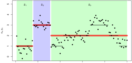
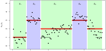
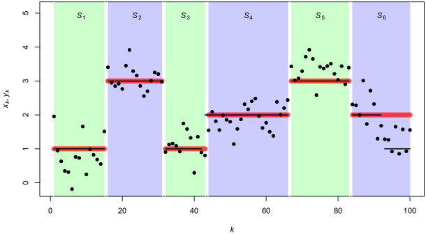
Figure 1: Some stages of QATS. Horizontal black lines represent the true, original path $\boldsymbol{x}^{o}$, whereas points correspond to the observation sequence $\boldsymbol{y}$. Top: After a few iterations of QATS, the best local path on $S_{1}$ with at most three segments is constant equal to $\widehat{z}_{1}=1$, indicated by the red line. The best local path on $S_{2}$ with at most three segments and previous states $\widehat{z}_{1}=1$ is constant equal to $\widehat{z}_{2}=3$ in red. The current segment under investigation is now $S_{3}$. Middle: In step (1), the search for the best local path on $S_{3}$ with at most three segments determines a path with $\widehat{c}=3$ segments (see Figure 2). This replaces the old segment $S_{3}$ by the new ones $S^{1}$, $S^{2}$, and $S^{3}$, and the scalar $\widehat{z}_{3}=1$ by the vector of states $(2,3,2)$. Step (2) now suggests to set the new $S_{3}$ as the current segment under investigation. Bottom: Step (1) indicated to replace the old $S_{3}$ by some new $S^{1}$ and $S^{2}$, and the old $\widehat{z}_{3}$ by $(1,2)$, whereas step (2) set the new $S_{3}$ as the current segment. Applying steps (1–2) to $S_{3}$, followed by $S_{4}$ and then $S_{5}$, does not yield any changes. The next interval under investigation will be $S_{6}$.

2.2 Approximation

To achieve sub-linear computational complexity in $n$, the search of the best local path with at most three segments on a given segment $S=\ell{:}r$ of length $d=r-\ell+1$ is only performed approximately, in the sense that the vector $\boldsymbol{x}\in{\cal X}^{d}$ with at most three segments and the highest local likelihood $\Lambda_{\ell:r}(\boldsymbol{x}|x_{0})$ may not be found exactly. Instead, we perform an approximation by comparing the best constant path $\boldsymbol{x}^{*1}$, the approximate best local paths (to be defined below) with two and three segments, respectively denoted $\tilde{\boldsymbol{x}}^{2}$ and $\tilde{\boldsymbol{x}}^{3}$, and selecting among those that path with the highest local likelihood score. The reasons for this approximation and the elements of our procedure are detailed in this section.

The search of the best constant path on $\ell{:}r$ with previous state $x_{0}\in{\cal X}$ consists in the following maximization problem

$$H^{1}\ :=\ \max_{i\in{\cal X}}\,\Lambda_{\ell:r}(\boldsymbol{x}_{\ell:r}(i)|x_{0}),$$ (2.3)

where

$$\boldsymbol{x}_{\ell:r}(i)\ :=\ i\cdot\boldsymbol{1}_{d}.$$

Note that the dependence on $\ell$, $r$ and $x_{0}$ for $H^{1}$ is omitted in order to facilitate notation, and is therefore implicit. The same principle will be used in the sequel when convenient.

The best constant path is the vector

$$\boldsymbol{x}^{*1}\ :=\ \boldsymbol{x}_{\ell:r}(i_{\ell:r}^{*}),\qquad\text{with}\quad i_{\ell:r}^{*}\ :=\ \mathop{\rm arg\,max}_{i\in{\cal X}}\,\Lambda_{\ell:r}(\boldsymbol{x}_{\ell:r}(i)|x_{0}).$$

This search costs $m$ evaluations of $\Lambda_{\ell:r}$ which, after preprocessing the data (see Section 2.3), is a feasible task since it is independent of $d$.

The search of the best path on $\ell{:}r$ with two or three segments is computationally more involved, because it involves the search of the respective maxima of the following two target functionals

$$H^{2}(k)\ :=\ \max_{\boldsymbol{i}\in{\cal X}^{2}:i_{1}\neq i_{2}}\,\Lambda_{\ell:r}(\boldsymbol{x}_{\ell:k:r}(\boldsymbol{i})|x_{0}),$$ (2.4)

$$H^{3}(\boldsymbol{k})\ :=\ \max_{\boldsymbol{i}\in{\cal X}^{3}:i_{1}\neq i_{2}\neq i_{3}}\,\Lambda_{\ell:r}(\boldsymbol{x}_{\ell:k_{1}:k_{2}:r}(\boldsymbol{i})|x_{0}),$$ (2.5)

over all $k\in{\cal K}^{2}_{\ell:r}$ and $\boldsymbol{k}\in{\cal K}^{3}_{\ell:r}$, where

$$\boldsymbol{x}_{\ell:k:r}(\boldsymbol{i})\ :=\ \bigl{(}i_{1}\cdot\boldsymbol{1}_{k-\ell},\,i_{2}\cdot\boldsymbol{1}_{r-k+1}\bigr{)},$$

$$\boldsymbol{x}_{\ell:k_{1}:k_{2}:r}(\boldsymbol{i})\ :=\ \bigl{(}i_{1}\cdot\boldsymbol{1}_{k_{1}-\ell},\,i_{2}\cdot\boldsymbol{1}_{k_{2}-k_{1}},\,i_{3}\cdot\boldsymbol{1}_{r-k_{2}+1}\bigr{)},$$

and

$${\cal K}^{2}_{\ell:r}\ :=\ \{k:\ell<k\leq r\},$$

$${\cal K}^{3}_{\ell:r}\ :=\ \{(k_{1},k_{2}):\ell<k_{1}<k_{2}\leq r\}.$$

Figure 2 depicts the natural logarithm of the two maps $H^{2}$ and $H^{3}$ in the context of Figure 1.

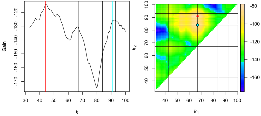
Figure 2: Plots of ${\cal H}^{2}=\log H^{2}$ (left) and ${\cal H}^{3}=\log H^{3}$ (right) in the setting of the top and middle plots of Figure 1, where the segment $\ell_{3}{:}r_{3}$ is under investigation. Black lines correspond to the true change points of the hidden chain $\boldsymbol{x}$, whereas the red line (left) and the red point (right) correspond to the respective global maxima of each map. The turquoise line (left) and turquoise diamond (right) correspond to the output of Algorithms 2 and 4, respectively.

Indeed, searching the global maximum of $H^{2}$, respectively $H^{3}$, would require $(r-\ell)m(m-1)$, respectively $(r-\ell)(r-\ell-1)m(m-1)^{2}/2$, probes of $\Lambda_{\ell:r}$. When $n$ and therefore $\ell{:}r$ are large, this task becomes computationally too costly, even after preprocessing the data (see Section 2.3). Consequently, we devise an approximate search algorithm to rapidly determine a one-dimensional local maximum of $H^{2}$ and a two-dimensional local maximum $H^{3}$, instead of their respective global maxima. Here, an index $k^{*}\in{\cal K}^{2}_{\ell:r}$ is called a one-dimensional local maximum of $H^{2}$ if $H^{2}(k^{*})\geq H^{2}(k)$ for $k\in{\cal K}^{2}_{\ell:r}$ such that $|k^{*}-k|=1$. Likewise, a pair of indices $\boldsymbol{k}^{*}\in{\cal K}^{3}_{\ell:r}$ is called a two-dimensional local maximum of $H^{3}$ if $H^{3}(\boldsymbol{k}^{*})\geq H^{3}(\boldsymbol{k})$ for $\boldsymbol{k}\in{\cal K}^{2}_{\ell:r}$ such that $\|\boldsymbol{k}^{*}-\boldsymbol{k}\|_{1}=1$, where we define $\|\boldsymbol{\xi}\|_{1}:=|\xi_{1}|+|\xi_{2}|$ for a vector $\boldsymbol{\xi}=(\xi_{1},\xi_{2})\in\mathbb{R}^{2}$.

The approximate search of the best paths with two and three segments is inspired by an adaptive search algorithm known as optimistic search (OS). OS was first used in detection of mean changes in independent Gaussian data by Kovács et al. (2020) in order to obtain sub-linear computational complexity when determining a potential new change point. In its simplest formulation, OS takes as an input a real-valued function $H$ defined on a segment $L{:}R$, a tuning parameter $\nu\in(0,1)$, and a maximal segment length $d_{o}>1$, and it returns a one-dimensional local maximum of $H$ on $L{:}R$. The pseudocode for this procedure is given in Algorithm 1. Essentially, OS checks the values of two points and keeps a segment that contains the point with a larger value. In this way, the kept segment contains at least one local maximum of $H$ on $\ell{:}r$. The choice of two points ensures that a proportion of at least $\nu/2$ is excluded from the search interval. Thus, OS finds a local maximum of $H$ on $\ell{:}r$ in ${\cal O}(\log(r-\ell))$ steps.

Lemma 2.1 (Kovács et al., 2020).

OS, as displayed in Algorithm 1, returns a local maximum $k^{*}\in L{:}R$ of $H$ in ${\cal O}(\log(R-L))$ steps/probes of $H$, and its $H$-value $h^{*}=H(k^{*})$, which is at least as large as any of the other probes performed during the algorithm.

Input: $L,R:L\leq R$, $M\in(L{:}R)\cup\{0\}$, $H:L{:}R\to\mathbb{R}$, $\nu\in(0,1)$, $d_{o}>1$

Output: $(k^{*},h^{*})$, a local maximum of $H$ and its $H$-value

if $M=0$ then $M\leftarrow\lfloor(L+\nu R)/(1+\nu)\rfloor$;

while $R-L\geq d_{o}$ do

        if $R-M>M-L$ then

               $W\leftarrow\lceil R-\nu(R-M)\rceil$

               if $H(W)>H(M)$ then $L\leftarrow M$ ; $M\leftarrow W$ else $R\leftarrow W$;

               

       else

               $W\leftarrow\lceil L+\nu(M-L)\rceil$

               if $H(W)>H(M)$ then $R\leftarrow M$ ; $M\leftarrow W$ else $L\leftarrow W$;

               

       

$h^{*}\leftarrow-\infty$

for $k\in L{:}R$ do

        if $H(k)>h^{*}$ then $(k^{*},h^{*})\leftarrow(k,H(k))$;

       

Algorithm 1 Optimistic search: $\mathrm{OS}(L,R,M,H,\nu,d_{o})$

For the remainder of this paper, we assume fixed values for the tuning parameter $\nu$ and the minimal segment length $d_{o}$, and therefore drop the dependence on those parameters when calling $\mathrm{OS}$.

2.2.1 One-dimensional optimistic search on $H^{2}$

To obtain a local maximum of $H^{2}$ over ${\cal K}^{2}_{\ell:r}$, simply set $H=H^{2}$, $L=\ell+1$, $R=r$ and apply OS. The resulting procedure, as displayed in Algorithm 2, requires ${\cal O}(\log(r-\ell))$ iterations and returns $k^{*}\in{\cal K}^{2}_{\ell:r}$ such that

$$\tilde{\boldsymbol{x}}^{2}\ :=\ \boldsymbol{x}_{\ell:k^{*}:r}(\boldsymbol{i}_{\ell:k^{*}:r}^{*}),$$

is an approximate best local path with two segments on $\ell{:}r$ and previous state $x_{0}$, with

$$\boldsymbol{i}_{\ell:k^{*}:r}^{*}\ :=\ \mathop{\rm arg\,max}_{\boldsymbol{i}\in{\cal X}^{2}:i_{1}\neq i_{2}}\,\Lambda_{\ell:r}(\boldsymbol{x}_{\ell:k^{*}:r}(\boldsymbol{i})|x_{0}).$$

Input: $\ell,r:r-\ell\geq 1$, $x_{0}\in{\cal X}$

Output: $(k^{*},h^{*})$, a local maximum of $H^{2}$ on ${\cal K}^{2}_{\ell:r}$ and its $H^{2}$-value

$(k^{*},h^{*})\leftarrow\mathrm{OS}\bigl{(}\ell+1,r,0,H^{2}\bigr{)}$

Algorithm 2 Optimistic search for $H^{2}$: $\mathrm{OSH}^{2}(\ell,r,x_{0})$

2.2.2 Two-dimensional optimistic search on $H^{3}$

The procedure is based on an alternation of the fixed and varying argument of $H^{3}$ and on the application of Algorithm 1 to the varying one.

Strategy.

The strategy for the two-dimensional optimistic search can be broken down in the following three steps:

Initialization:

Initialize $h_{\mathrm{old}}$ and $h_{\mathrm{new}}$ to $-\infty$ and set some arbitrary index $k_{o}\in(\ell+2){:}r$. We also set the initial solution $\boldsymbol{k}^{*}$ to have $k_{o}$ as a second component, i.e. $k_{2}^{*}=k_{o}$.

Horizontal search:

For the first iteration or as long as $h_{\mathrm{old}}$ is strictly smaller than $h_{\mathrm{new}}$, we proceed as follows: Update $h_{\mathrm{old}}\leftarrow h_{\mathrm{new}}$ and apply OS to the function $H(k)=H^{3}(k,k_{2}^{*})$ defined for $k\in L{:}R=(\ell+1){:}(k_{2}^{*}-1)$ using the current value of $k_{1}^{*}$ as the first probe point (i.e. $M=k_{1}^{*}$ in the first step of OS), for all but the first iteration, for which the default initial probe is used. This so-called horizontal search yields an index $k^{*}$ which is a local maximum of $H$ and which replaces the old value of $k_{1}^{*}$. It also returns the score $h_{\mathrm{new}}$ of that new $\boldsymbol{k}^{*}$.

Vertical search:

If $h_{\mathrm{old}}$ is still strictly smaller than $h_{\mathrm{new}}$ (which is necessarily the case for the first iteration), we perform a vertical search: Update $h_{\mathrm{old}}\leftarrow h_{\mathrm{new}}$ and apply OS to the function $H(k)=H^{3}(k_{1}^{*},k)$ defined for $k\in L{:}R=(k_{1}^{*}+1){:}r$ using the current value of $k_{2}^{*}$ as the first probe point (i.e. $M=k_{2}^{*}$ in the first step of OS). This yields an index $k^{*}$ which is a local maximum of $H$ and which replaces the old value of $k_{2}^{*}$, as well as the score $h_{\mathrm{new}}$ of that new $\boldsymbol{k}^{*}$.

Unless the new score is no larger than the old one at a certain stage, we alternate between the horizontal and vertical searches, swapping the roles of the fixed and varying components of $H^{3}$ and applying OS to the varying one.

This alternating procedure strictly increases the score at each iteration, unless two consecutive iterations yield the same score, in which case a local maximum of $H^{3}$ has been found. Indeed, because the current best index of the varying component of $H^{3}$ is used as the first probe point $M$ of OS, this ensures that any update of $M$ in the while-loop of OS strictly increases the score. In contrast, if $M$ remains unchanged in the while-loop and is returned at the end of the for-loop, then $\boldsymbol{k}^{*}$ has not been updated twice in a row. Consequently, $k_{1}^{*}$ is a “vertical local maximum” of $H^{3}(\cdot,k_{2}^{*})$ and $k_{2}^{*}$ is a “horizontal local maximum” of $H^{3}(k_{1}^{*},\cdot)$. In other words, $\boldsymbol{k}^{*}$ is a two-dimensional local maximum of $H^{3}$.

Lemma 2.2.

Let $V:{\cal K}^{3}_{\ell:r}\to\mathbb{R}$ and suppose that every one-dimensional local maximum of $V$ lies on an $s\times s$ grid, namely, there exists a subset ${\cal K}$ of $(\ell+1){:}r$ with cardinality $s$ such that:

(i) For every $k_{1}\in(\ell+1){:}(r-1)$, all local maxima of $V(k_{1},\cdot)$ on $(k_{1}+1){:}r$ are in ${\cal K}$;

(ii) For every $k_{2}\in(\ell+2){:}r$, all local maxima of $V(\cdot,k_{2})$ on $(\ell+1){:}(k_{2}-1)$ are in ${\cal K}$.

Then, the alternation of horizontal and vertical searches returns a two-dimensional local maximum of $V$ on ${\cal K}^{3}_{\ell:r}$ in ${\cal O}\bigl{(}s^{2}\log(r-\ell)\bigr{)}$ probes of $V$.

It will be shown (Section 3.1; cf. Figure 3) that the function $H^{3}$ defined in (2.5) fulfills the conditions of 2.2 in a noiseless scenario. The specific set ${\cal K}$ is shown to be $\{\kappa_{1},\ldots,\kappa_{c-1}\}$, where each $\kappa_{a}$ is a true change point. In consequence, the alternating procedure returns a pair $\boldsymbol{k}^{*}$ consisting of two true change points. An alternative way to treat vertical and horizontal searches which takes into account boundary effects is presented in Section A.2.

Diagonal elements.

If the alternation of OS terminates at an element $\boldsymbol{k}^{*}$ belonging to the diagonal of ${\cal K}^{3}_{\ell:r}$, then that $\boldsymbol{k}^{*}$ is in general a local maximum of $H^{3}$, but there might be a point somewhere else on the diagonal with a strictly larger $H^{3}$-score to which it would be suitable to move. Thus, in such a scenario, we proceed alternatively: Apply OS to the function $(\ell+1){:}(r-1)\ni k\mapsto H^{3}(k,k+1)$ with $k_{1}^{*}$ as the first probe point, resulting in an element $k^{*}$ and a (non-necessarily strict) increase of the score. Once $\boldsymbol{k}^{*}$ has been updated to the new pair $(k^{*},k^{*}+1)$, the alternation between horizontal and vertical searches proceeds as explained earlier.

Maximum number of alternations.

To prevent the algorithm from performing too many alternations between horizontal and vertical searches, we stop it if the number of iterations exceeds a certain threshold $v_{o}$. Our experiments show that $v_{o}=20$ performs well. Should the algorithm terminate from this stopping criteria, it will then return the last update of $\boldsymbol{k}^{*}$ along with its corresponding $H^{3}$-score. Note that this latter element has no guarantee of being a local maximum of $H^{3}$, but is necessarily the element with the largest $H^{3}$-score of all elements visited so far, including all the probes performed by OS.

Input: $\ell,r:r-\ell\geq 2$, $x_{0}\in{\cal X}$, $v_{o}>1$, $k_{o}\in(\ell+2){:}r$

Output: $(\boldsymbol{k}^{*},h^{*})$, an element of ${\cal K}^{3}_{\ell:r}$ and its $H^{3}$-value

$\boldsymbol{k}^{*}\leftarrow(\ell+1,k_{o})$

$h_{\mathrm{old}}\leftarrow h_{\mathrm{new}}\leftarrow-\infty$

$\tau\leftarrow 0$ ($0=\text{horizontal}$, $1=\text{vertical}$)

$v\leftarrow 1$

while ($h_{\mathrm{old}}<h_{\mathrm{new}}$ and $v<v_{o}$) or $v=1$ do

        $h_{\mathrm{old}}\leftarrow h_{\mathrm{new}}$

        if $\tau=0$ then

               $(k_{1}^{*},h^{*})\leftarrow\mathrm{OS}\bigl{(}\ell+1,k^{*}_{2}-1,k_{1}^{*},H^{3}(\cdot,k^{*}_{2})\bigr{)}$

       else

               $(k_{2}^{*},h^{*})\leftarrow\mathrm{OS}\bigl{(}k_{1}^{*}+1,r,k_{2}^{*},H^{3}(k^{*}_{1},\cdot)\bigr{)}$

       if $k_{1}^{*}+1=k_{2}^{*}$ then

               $(k^{*},h^{*})\leftarrow\mathrm{OS}\bigl{(}\ell+1,r-1,k_{1}^{*},k\mapsto H^{3}(k,k+1)\bigr{)}$

               $\boldsymbol{k}^{*}\leftarrow(k^{*},k^{*}+1)$

       $h_{\mathrm{new}}\leftarrow h^{*}$

        $\tau\leftarrow 1-\tau$ (change direction)

        $v\leftarrow v+1$

       

Algorithm 3 Seeded optimistic search for $H^{3}$: $\mathrm{sOSH}^{3}(\ell,r,x_{0},v_{o},k_{o})$

Complete two-dimensional search.

The procedure, as described to this point and which relies on an initial seed $k_{o}\in(\ell+2){:}r$, is summarized in Algorithm 3. Now we choose $n_{\mathrm{seeds}}\geq 1$ evenly spaced starting points $k_{o}\in(\ell+2){:}r$, run Algorithm 3 for each of those seeds, and select the endpoint $\boldsymbol{k}^{*}$ with the largest $H^{3}$-score. This method allows to increase the chance of finding an element $\boldsymbol{k}^{*}\in{\cal K}^{3}_{\ell:r}$ with a large value of $H^{3}$. Simulations showed that $n_{\mathrm{seeds}}=3$ is a good trade-of between speed and exploration of the space ${\cal K}^{3}_{\ell:r}$.

The complete procedure is summarized in Algorithm 4. It returns $\boldsymbol{k}^{*}\in{\cal K}^{3}_{\ell:r}$ such that

$$\tilde{\boldsymbol{x}}^{3}\ :=\ \boldsymbol{x}_{\ell:k^{*}_{1}:k^{*}_{2}:r}(\boldsymbol{i}_{\ell:k^{*}_{1}:k^{*}_{2}:r}^{*}),$$

is an approximate best local path with three segments on $\ell{:}r$ and previous state $x_{0}$, where

$$\boldsymbol{i}_{\ell:k^{*}_{1}:k^{*}_{2}:r}^{*}\ :=\ \mathop{\rm arg\,max}_{\boldsymbol{i}\in{\cal X}^{3}:i_{1}\neq i_{2}\neq i_{3}}\,\Lambda_{\ell:r}(\boldsymbol{x}_{\ell:k^{*}_{1}:k^{*}_{2}:r}(\boldsymbol{i})|x_{0}).$$

Input: $\ell,r:r-\ell\geq 2$, $x_{0}\in{\cal X}$, $v_{o}>1$, $n_{\mathrm{seeds}}\in 1{:}(r-\ell-1)$

Output: $(\boldsymbol{k}^{*},h^{*})$, an element of ${\cal K}^{3}_{\ell:r}$ and its $H^{3}$-value

$h^{*}\leftarrow-\infty$

for $i\in 1{:}n_{\mathrm{seeds}}$ do

        $k_{o}\leftarrow\ell+2+\lfloor i\cdot(r-\ell-1)/(n_{\mathrm{seeds}}+1)\rfloor$

        $(\boldsymbol{k}^{\mathrm{temp}},h^{\mathrm{temp}})\leftarrow\mathrm{sOSH}^{3}(\ell,r,x_{0},v_{o},k_{o})$

        if $h^{\mathrm{temp}}>h^{*}$ then $(\boldsymbol{k}^{*},h^{*})\leftarrow(\boldsymbol{k}^{\mathrm{temp}},h^{\mathrm{temp}})$;

       

Algorithm 4 Optimistic search for $H^{3}$: $\mathrm{OSH}^{3}(\ell,r,x_{0},v_{o},n_{\mathrm{seeds}})$

2.3 Linearization

The maximizations in (2.3) to (2.5) needed to compute $H^{c}$, $c\in 1{:}3$, involve the evaluation of $\Lambda_{\ell:r}$ at $\boldsymbol{x}_{\ell:r}(i)$, $\boldsymbol{x}_{\ell:k:r}(\boldsymbol{i})$ and $\boldsymbol{x}_{\ell:k_{1}:k_{2}:r}(\boldsymbol{i})$, but those can be greatly simplified if we assume the following:

Assumption 1.

For all $k\in 1{:}n$ and $i\in 1{:}m$, we have that $f_{i}(y_{k})>0$.

Indeed, consider for instance the computation of $\Lambda_{\ell:r}(\boldsymbol{x}_{\ell:k:r}(\boldsymbol{i})|x_{0})$ when $\ell>1$. We have that

$$\Lambda_{\ell:r}(\boldsymbol{x}_{\ell:k:r}(\boldsymbol{i})|x_{0})\ =\ p_{x_{0}i_{1}}p_{i_{1}i_{1}}^{k-\ell-1}p_{i_{1}i_{2}}p_{i_{2}i_{2}}^{r-k}\left(\prod_{t=\ell}^{k-1}f_{i_{1}}(y_{t})\right)\left(\prod_{t=k}^{r}f_{i_{2}}(y_{t})\right).$$ (2.6)

If we now define the following matrix $\boldsymbol{F}$ of cumulative products

$$\boldsymbol{F}\ =\ (F_{ik})_{i\in{\cal X},k\in 1:n}\ :=\ \left(\prod_{t=1}^{k}f_{i}(y_{t})\right)_{i\in{\cal X},k\in 1:n},$$

then, under 1, expression (2.6) simplifies to

$$\Lambda_{\ell:r}(\boldsymbol{x}_{\ell:k:r}(\boldsymbol{i})|x_{0})\ =\ p_{x_{0}i_{1}}p_{i_{1}i_{1}}^{k-\ell-1}p_{i_{1}i_{2}}p_{i_{2}i_{2}}^{r-k}\frac{F_{i_{1},k-1}}{F_{i_{1},\ell-1}}\frac{F_{i_{2},r}}{F_{i_{2},k-1}}.$$

In other words, precomputing the matrix $\boldsymbol{F}$ in ${\cal O}(mn)$ operations and memory allows to compute any $\Lambda_{\ell:r}(\boldsymbol{x}_{\ell:r}(i)|x_{0})$, $\Lambda_{\ell:r}(\boldsymbol{x}_{\ell:k:r}(\boldsymbol{i})|x_{0})$ or $\Lambda_{\ell:r}(\boldsymbol{x}_{\ell:k_{1}:k_{2}:r}(\boldsymbol{i})|x_{0})$ in just ${\cal O}(1)$ operations, that is, independently of the size of $\ell{:}r$, and therefore $n$. This gives rise to the following Lemma:

Lemma 2.3.

Under 1, the computational costs of evaluating $H^{1}$, $H^{2}(k)$ and $H^{3}(\boldsymbol{k})$ are respectively ${\cal O}(m)$, ${\cal O}(m^{2})$ and ${\cal O}(m^{3})$.

Now, in order to prevent numerical instability due to multiplication and division of small quantities, we linearize all relevant expressions by applying the natural logarithm. Precisely, the matrices

$$\boldsymbol{q}\ =\ (q_{ij})_{i,j\in{\cal X}}\ :=\ \left(\log p_{ij}\right)_{i,j\in{\cal X}},$$

$$\boldsymbol{G}\ =\ \left(G_{ik}\right)_{i\in{\cal X},\,k\in 1{:}n}\ :=\ \left(\sum_{t=1}^{k}\log f_{i}(y_{t})\right)_{i\in{\cal X},\,k\in 1{:}n},$$ (2.7)

characterize completely the log-local likelihood scores $\log\Lambda_{\ell:r}(\boldsymbol{x}_{\ell:r}(i)|x_{0})$, $\log\Lambda_{\ell:r}(\boldsymbol{x}_{\ell:k:r}(\boldsymbol{i})|x_{0})$ and $\log\Lambda_{\ell:r}(\boldsymbol{x}_{\ell:k_{1}:k_{2}:r}(\boldsymbol{i})|x_{0})$, see Section A.3. Now, we replace $H^{1}$ by

$${\cal H}^{1}\ :=\ \max_{i\in{\cal X}}\,\log\Lambda_{\ell:r}(\boldsymbol{x}_{\ell:r}(i)|x_{0}),$$

and, in Algorithms 2 and 4, we replace $H^{2}$ and $H^{3}$ by

$${\cal H}^{2}(k)\ :=\ \max_{\boldsymbol{i}\in{\cal X}^{2}:i_{1}\neq i_{2}}\,\log\Lambda_{\ell:r}(\boldsymbol{x}_{\ell:k:r}(\boldsymbol{i})|x_{0})$$

$${\cal H}^{3}(\boldsymbol{k})\ :=\ \max_{\boldsymbol{i}\in{\cal X}^{3}:i_{1}\neq i_{2}\neq i_{3}}\,\log\Lambda_{\ell:r}(\boldsymbol{x}_{\ell:k_{1}:k_{2}:r}(\boldsymbol{i})|x_{0}),$$

respectively. The above two maps are displayed in Figure 2.

Corollary 2.4.

Under 1, the computational costs of ${\cal H}^{1}$, ${\cal H}^{2}(k)$ and ${\cal H}^{3}(\boldsymbol{k})$ are respectively ${\cal O}(m)$, ${\cal O}(m^{2})$ and ${\cal O}(m^{3})$.

2.4 Complete algorithm

The pseudocode of the complete Quick Adaptive Ternary Segmentation (QATS) algorithm as described in Section 2.1 is given in Algorithm 5. It necessitates the preprocessing of data from Section 2.3 and it makes use of Algorithms 2 and 4 for which the $H$-maps are replaced by their log-versions, i.e. the calligraphic letters ${\cal H}$. The QATS-path $\widehat{\boldsymbol{x}}$ is then be built from $\SS$ and $\widehat{\boldsymbol{z}}$ as in (2.2).

Input: $\log\boldsymbol{\pi}$, $\boldsymbol{q}$, $\boldsymbol{G}$, $v_{o}>1$, $n_{\mathrm{seeds}}\in 1{:}(r-\ell-1)$

Output: $(\SS,\widehat{\boldsymbol{z}})$, a segmentation of $1{:}n$ and the corresponding state values

$\SS\leftarrow(1{:}n)$ ; $\widehat{\boldsymbol{z}}\leftarrow 1$ ; $s\leftarrow 1$

$u\leftarrow 1$

while $u\leq s$ do

        $(\ell{:}r)\leftarrow S_{u}$

        if $u>1$ then $x_{0}\leftarrow\widehat{z}_{u-1}$;

        $(h^{*}_{1},h^{*}_{2},h^{*}_{3})\leftarrow({\cal H}^{1},-\infty,-\infty)$

        if $r-\ell\geq 1$ then

               $(k^{*},h^{*}_{2})\leftarrow\mathrm{OSH}^{2}(\ell,r,x_{0})$

               if $r-\ell\geq 2$ then

                      $(\boldsymbol{k}^{*},h^{*}_{3})\leftarrow\mathrm{OSH}^{3}(\ell,r,x_{0},v_{o},n_{\mathrm{seeds}})$

              

       $\widehat{c}\leftarrow\mathop{\rm arg\,max}_{c}\,h^{*}_{c}$

        if $\widehat{c}=1$ then $\widehat{z}_{u}\leftarrow i_{\ell:r}^{*}$ ; $u\leftarrow u+1$;

        if $\widehat{c}=2$ then $S_{u}\leftarrow(\ell{:}(k^{*}-1),k^{*}{:}r)$ ; $\widehat{z}_{u}\leftarrow\boldsymbol{i}_{\ell:k^{*}:r}^{*}$ ; $s\leftarrow s+1$;

        if $\widehat{c}=3$ then $S_{u}\leftarrow(\ell{:}(k^{*}_{1}-1),k^{*}_{1}{:}(k^{*}_{2}-1),k^{*}_{2}{:}r)$ ; $\widehat{z}_{u}\leftarrow\boldsymbol{i}_{\ell:k^{*}_{1}:k^{*}_{2}:r}^{*}$ ; $s\leftarrow s+2$;

       

Algorithm 5 Quick Adaptive Ternary Segmentation: $\mathrm{QATS}(\log\boldsymbol{\pi},\boldsymbol{q},\boldsymbol{G},v_{o},n_{\mathrm{seeds}})$

2.5 Computational complexity

The Lemma below provides a bound on the number of iterations of QATS as displayed in Algorithm 5. It involves the number $s$ of segments in $\SS$ returned by QATS.

Lemma 2.5.

The number of iterations in the while loop of QATS is at most $2s-1$.

Proof.

In the worst case, each of the $s-1$ separations of $1{:}n$ is due to single splits ($\widehat{c}=2$), and no double splits ($\widehat{c}=3$). Then, to confirm that on each segment of $\SS$, the best local path with at most three segments is constant, one extra iteration ($\widehat{c}=1$) per segment is necessary. ∎

Consequently, the number of calls of procedure $\mathrm{OSH}^{2}$ and the number of calls of procedure $\mathrm{OSH}^{3}$ are both bounded by $2s-1$. 2.1 implies that the number of probes of ${\cal H}^{2}$ in $\mathrm{OSH}^{2}$ for a given segment $\ell{:}r$ is of the order ${\cal O}(\log(r-\ell))$. As to the complexity of $\mathrm{OSH}^{3}$, it is broken down as follows: First, for each call of $\mathrm{OSH}^{3}$, there are $n_{\mathrm{seeds}}$ calls of $\mathrm{sOSH}^{3}$. Second, the number of alternations of vertical and horizontal searches in $\mathrm{sOSH}^{3}$ for a given seed, and therefore the number of calls of $\mathrm{OS}$, is bounded by $v_{o}$, since Algorithm 3 stops as soon as the number $v$ of alternations exceeds $v_{o}$ (with $v_{o}=20$ performing well). Then again, for each call of $\mathrm{OS}$, the number of probes of ${\cal H}^{3}$ is of the order ${\cal O}(\log(r-\ell))$. Finally, 2.4 ensures that each query ${\cal H}^{c}$ costs ${\cal O}(m^{c})$ operations, $c\in 1{:}3$. This reasoning proves the following result:

Theorem 2.6.

QATS has computational complexity ${\cal O}(sm^{3}\log n)$.

Note first that QATS performs particularly well with only a few segments in contrast to dynamic programming methods, which work independently of the number of segments. Second, the benefits of QATS are more pronounced for small values of $m$, namely, $m\ll n/s$. Finally, the process of storing the data has computational complexity ${\cal O}(mn)$ and is easily parallelized, e.g. via the parallel-scan algorithm (Ladner and Fischer, 1980), resulting in $O(\log n)$ span complexity. That means, the overall complexity (without parallelization and proper storing of the data) is ${\cal O}\bigl{(}\max(mn,sm^{3}\log n)\bigr{)}$, where ${\cal O}(mn)$ is due to the computation of the input $\boldsymbol{G}$ from the raw data.

3 Theoretical analysis

In this section, we investigate theoretical properties of QATS, and, for technical simplicity, we focus on HMMs with two hidden states (formalized in 2 below).

3.1 Justification

At each step of QATS, a given segment may be split in two or three new segments with the change point(s) being determined by the search of local maxima on ${\cal H}^{2}$ and ${\cal H}^{3}$. To justify this procedure, we show that there is indeed a one-to-one correspondence between local maxima of ${\cal H}^{2}$ and ${\cal H}^{3}$, and change points of the hidden signal. In the sequel, we study without loss of generality the case of $\ell=1$ and $r=n$, and therefore drop any dependence on $\ell$ and $r$ in the notation.

Let $\boldsymbol{x}^{o}$ be the true signal at the origin of the observations $\boldsymbol{y}$. Let ${\cal K}^{o}:=\{k\in 2{:}n:x_{k-1}\neq x_{k}\}$ be the set of true change points of $\boldsymbol{x}^{o}$. That means, $\boldsymbol{x}^{o}$ consists of $s^{o}=\#{\cal K}^{o}+1$ segments. If $s^{o}>1$, the elements of ${\cal K}^{o}$ are written $\kappa_{1}<\cdots<\kappa_{s^{o}-1}$. For convenience, we also define $\kappa_{0}:=1$ and $\kappa_{s^{o}}:=n+1$. Finally, we set a basic setting for which a mathematical analysis of ${\cal H}^{2}$ and ${\cal H}^{3}$ is tractable:

Assumption 2.

We have that $n\geq 3$, $m=2$, $\boldsymbol{\pi}=(1/2,1/2)$ and $p_{12}=p_{21}=\varepsilon$ for some $\varepsilon\in(0,1/2)$. Furthermore, ${\cal Y}=\mathbb{R}$ and there exist constants $\beta_{1},\beta_{2}\in\mathbb{R}$, $\beta_{2}>0$, such that:

$$\{y_{k}:k\in 1{:}n\}\ \in\ 1{:}2,$$

$$g_{i}(y):=\log f_{i}(y)\ =\ \beta_{1}+\beta_{2}1_{[y=i]}, i,y\in 1{:}2,$$

$$g_{x^{o}_{k}}(y_{k})\ =\ \beta_{1}+\beta_{2}, k\in 1{:}n.$$

Remark 3.1.

The setting described by 2 can be thought of as the ideal case where the observation sequence $\boldsymbol{y}$ completely characterizes the true signal $\boldsymbol{x}^{o}$. Furthermore, in this setting, the probability that the underlying Markov chain stays at a certain state is higher than that of jumping to another state, since $p_{11}=p_{22}=1-\varepsilon>1/2$.

Example 3.2.

2 holds, for instance, when ${\cal L}(Y_{k}|X_{k}=i)={\cal N}(i,\sigma^{2})$, $i\in 1{:}2$, for some $\sigma>0$, since then $\beta_{1}=-(\log(2\pi\sigma^{2})+\sigma^{-2})/2$ and $\beta_{2}=\sigma^{-2}/2$ satisfy the latter two properties.

In the following Lemma, we show that local maxima of ${\cal H}^{2}$ and ${\cal H}^{3}$ in the interior of ${\cal K}^{2}$ and ${\cal K}^{3}$ provide information on change points. Reciprocally, we prove that all change points appear either as local maxima of ${\cal H}^{2}$ or as components of local maxima of ${\cal H}^{3}$. In other words, the study of the maps ${\cal H}^{2}$ and ${\cal H}^{3}$ shall theoretically unveil all change points of the true sequence $\boldsymbol{x}^{o}$.

Theorem 3.3.

Suppose that $s^{o}\geq 2$ and that 2 holds. Then:

(i) Local maxima of ${\cal H}^{2}$ are located either at $2$, $n$ or $\kappa_{a}$, $a\in 1{:}(s^{o}-1)$. Local maxima of ${\cal H}^{3}$ are located either at boundary points $(2,n)$, $(2,\kappa_{a})$, $(\kappa_{a},n)$, $a\in 1{:}(s^{o}-1)$, on the diagonal $\{\boldsymbol{k}\in{\cal K}^{3}:k_{2}=k_{1}+1\}$, or at pairs $(\kappa_{a},\kappa_{b})$ with $a,b\in 1{:}(s^{o}-1)$ such that $a<b$ and $a+b$ is odd.

(ii) Conversely, for all $a\in 1{:}(s^{o}-1)$, either $(\kappa_{a-1},\kappa_{a})$ or $(\kappa_{a},\kappa_{a+1})$ is a local maximum of ${\cal H}^{3}$. (Note that $(\kappa_{0},\kappa_{1})$ or $(\kappa_{s^{o}-1},\kappa_{s^{o}})$ is a local maximum of ${\cal H}^{3}$ if and only if $\kappa_{1}$ or $\kappa_{s^{o}-1}$ is a local maximum of ${\cal H}^{2}$, respectively.)

Figure 3 exemplifies the above result. Part (i) of 3.3 indicates that the local maxima found by QATS serve as proper estimates of change points (cf. Lemmas 2.1 and 2.2). Conversely, as shown in the left panel of Figure 3, not every change point corresponds to a local maxima of ${\cal H}^{2}$. However, by Part (ii) of 3.3, the collection of maxima of ${\cal H}^{3}$ allows us to find all change points. We stress that this is one of the motivations for QATS, which uses three segments, instead of two as it is usually done in change point detection.

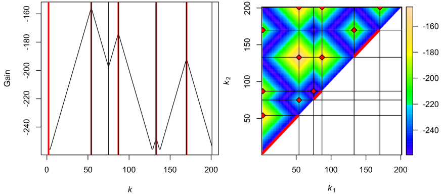
Figure 3: Plots of ${\cal H}^{2}=\log H^{2}$ (left) and ${\cal H}^{3}=\log H^{3}$ (right). Local maxima (in red) are located either on the boundaries, on the diagonal (for ${\cal H}^{3}$), on true change points or pairs thereof (black lines).

3.2 Sensitivity

At each iteration of the while loop of Algorithm 5, a local maximum $k^{*}$ of ${\cal H}^{2}$ may be added to the list of change points if the local likelihood score of a path with two segments and jump at $k^{*}$ is better than that of a constant path. Likewise, a local maximum $\boldsymbol{k}^{*}$ of ${\cal H}^{3}$ may be added to the list of change points if the local likelihood score of a path with three segments and jumps at $\boldsymbol{k}^{*}$ is better than that of a constant path. The following results derive conditions on the relative position of change points in order for corresponding paths with two or three segments to have a higher local likelihood score than that of a constant path. It also shows that if there is no change point ($s^{o}=1$), then the constant path indeed has a higher local likelihood score than any other path with two or three segments.

Define

$$\delta\ =\ \delta(\varepsilon,\beta_{2})\ :=\ \frac{1}{\beta_{2}}\log\left(\frac{1-\varepsilon}{\varepsilon}\right)\ >\ 0.$$

Lemma 3.4.

Suppose that 2 holds.

When $s^{o}=1$, we have ${\cal H}^{1}>\max_{k\in{\cal K}^{2}}\,{\cal H}^{2}(k)>\max_{\boldsymbol{k}\in{\cal K}^{3}}\,{\cal H}^{3}(\boldsymbol{k})$.

When $s^{o}=2$, we have ${\cal H}^{2}(\kappa_{1})>\max_{\boldsymbol{k}\in{\cal K}^{3}}\,{\cal H}^{3}(\boldsymbol{k})$ and the equivalence

$${\cal H}^{2}(\kappa_{1})\ >\ {\cal H}^{1}\quad\Leftrightarrow\quad\kappa_{1}\in\bigl{(}1+\delta,n+1-\delta\bigr{)}.$$

When $s^{o}=3$, we have the following equivalences

$${\cal H}^{2}(\kappa_{1})\ >\ {\cal H}^{1}\quad \Leftrightarrow\quad\kappa_{2}>\frac{n}{2}+1+\delta\quad\text{and}\quad\kappa_{1}\in\bigl{(}1+\delta,2\kappa_{2}-n-1-\delta\bigr{)},$$

$${\cal H}^{2}(\kappa_{2})\ >\ {\cal H}^{1}\quad \Leftrightarrow\quad\kappa_{1}<\frac{n}{2}+1-\delta\quad\text{and}\quad\kappa_{2}\in\bigl{(}2\kappa_{1}-1+\delta,n+1-\delta\bigr{)},$$

$${\cal H}^{3}(\kappa_{1},\kappa_{2})\ >\ {\cal H}^{1}\quad \Leftrightarrow\quad\kappa_{2}-\kappa_{1}\in(2\delta,n-2\delta),$$

$${\cal H}^{3}(\kappa_{1},\kappa_{2})\ >\ \max_{k\in{\cal K}^{2}}\,{\cal H}^{2}(k)\quad \Leftrightarrow\quad\kappa_{1}>1+\delta,\quad\kappa_{2}<n+1-\delta,\quad\text{and}\quad\kappa_{2}-\kappa_{1}\geq\delta-1.$$

Lemma 3.5.

Suppose that 2 holds and let $s^{o}\geq 3$ and $a\in 1{:}(s^{o}-1)$. Then ${\cal H}^{2}(\kappa_{a})>{\cal H}^{1}$ if, and only if,

$$\frac{\|\boldsymbol{y}_{1:(\kappa_{a}-1)}-i_{1}\cdot\boldsymbol{1}\|_{1}}{\kappa_{a}-1}\ <\ \frac{1}{2}-\frac{1}{2}\cdot\frac{\delta}{\kappa_{a}-1},$$

$$\frac{\|\boldsymbol{y}_{\kappa_{a}:n}-i_{2}\cdot\boldsymbol{1}\|_{1}}{n-\kappa_{a}+1}\ <\ \frac{1}{2}-\frac{1}{2}\cdot\frac{\delta}{n-\kappa_{a}+1},$$

for some $(i_{1},i_{2})\in\{(1,2),(2,1)\}$.

Lemma 3.6.

Suppose that 2 holds, and let $s^{o}\geq 3$ and $a,b\in 1{:}(s^{o}-1)$ be such that $a<b$ and $a+b$ is odd. Then ${\cal H}^{3}(\kappa_{a},\kappa_{b})>{\cal H}^{1}$ if, and only if,

$$\frac{\|\boldsymbol{y}_{1:(\kappa_{a}-1)}-i_{1}\cdot\boldsymbol{1}\|_{1}+\|\boldsymbol{y}_{\kappa_{b}:n}-i_{1}\cdot\boldsymbol{1}\|_{1}}{n-(\kappa_{b}-\kappa_{a})}\ <\ \frac{1}{2}-\frac{\delta}{n-(\kappa_{b}-\kappa_{a})},$$

$$\frac{\|\boldsymbol{y}_{\kappa_{a}:(\kappa_{b}-1)}-i_{2}\cdot\boldsymbol{1}\|_{1}}{\kappa_{b}-\kappa_{a}}\ <\ \frac{1}{2}-\frac{\delta}{\kappa_{b}-\kappa_{a}},$$

for some $(i_{1},i_{2})\in\{(1,2),(2,1)\}$.

3.3 Properties of QATS-paths

The path $\widehat{\boldsymbol{x}}$ returned by Algorithm 5 is admissible, in the sense that all transitions in $\widehat{\boldsymbol{x}}$ have positive probability. This is due to the fact that $\widehat{\boldsymbol{x}}$ is built from the left to the right, always taking into account the last state $x_{0}$ from the previous segment for the derivations.

The QATS-path is different from paths resulting from the risk-based segmentation techniques MAP, PMAP and sMAP mentioned in Section 1, as it does not maximize a risk function. Instead, it may be seen as a form of “greedy” decoder since it selects a window of observation $\ell{:}r$ and attempts to determine the best path with at most three segments in that window.

In consequence, if one omits the approximation due to OS in Algorithm 5, the resulting path is, by definition, an element of the following set

$$\widehat{{\cal X}}\ :=\ \left\{\boldsymbol{x}\in{\cal X}^{n}:\Lambda_{\ell_{u}:r_{u}}(\boldsymbol{x}_{\ell_{u}:r_{u}}|x_{\ell_{u}-1})\geq\Lambda_{\ell_{u}:r_{u}}(\boldsymbol{x}^{\prime}|x_{\ell_{u}-1}),\ \text{ for all }\boldsymbol{x}^{\prime}\in\bar{{\cal X}}^{d_{u}},\text{ and all }u\in 1{:}s\right\},$$

where $\bar{{\cal X}}^{d}$ denotes the set of vectors of size $d$ with at most three segments, and the elements $\ell_{u}$, $r_{u}$ and $d_{u}$ depend on the segmentation of the concerned $\boldsymbol{x}$. In particular, $\widehat{{\cal X}}$ does not contain vectors $\boldsymbol{x}$ for which there exists a certain segment $\ell_{u}{:}r_{u}$ which could be further split in two or three segments and at the same time yield a higher local likelihood score.

The next simple example shows that in general this set may contain more than one element.

Example 3.7.

Let $n=4$, $m=2$ and ${\cal L}(Y_{k}|X_{k}=i)={\cal N}(i,4)$. We further set $\log\boldsymbol{\pi}=\theta_{\boldsymbol{\pi}}\boldsymbol{1}$ and $\boldsymbol{q}=\theta_{\boldsymbol{q}}+\log 2\cdot\boldsymbol{i}$, with constants $\theta_{\boldsymbol{\pi}}=-\log 2$ and $\theta_{\boldsymbol{q}}=-\log 3$. Suppose now that we observe $\boldsymbol{y}=(1,4,-1,1)$. That means, with $\theta_{\boldsymbol{g}}=-\log(2\pi\sigma^{2})/2$, we have

$$\boldsymbol{G}\ =\ \theta_{\boldsymbol{g}}-\frac{1}{8}\begin{pmatrix}0&9&4&0\\ 1&4&9&1\end{pmatrix}.$$

Simple computations show that the best paths on $1{:}n$ with one, two or three segments are the following paths, respectively, along with their corresponding log-local likelihood scores:

$$\boldsymbol{x}^{(1)}\ :=\ (1,1,1,1):\quad \quad\log\Lambda_{1:n}(\boldsymbol{x}^{(1)})\ =\ \theta-13/8+3\log 2,$$

$$\boldsymbol{x}^{(2)}\ :=\ (2,2,1,1):\quad \quad\log\Lambda_{1:n}(\boldsymbol{x}^{(2)})\ =\ \theta-9/8+2\log 2,$$

$$\boldsymbol{x}^{(3)}\ :=\ (1,2,1,1):\quad \quad\log\Lambda_{1:n}(\boldsymbol{x}^{(3)})\ =\ \theta-8/8+\log 2,$$

where $\theta=\theta_{\boldsymbol{\pi}}+3\theta_{\boldsymbol{q}}+4\theta_{\boldsymbol{g}}$. But since $\log 2\approx 0.69>4/8$ and $2\log 2\approx 1.39>5/8$, we find that $\boldsymbol{x}^{(1)}$ is the best path with at most three segments, thus implying $(1,1,1,1)\in\widehat{{\cal X}}$.

Let us now prove that $(2,2,1,1)\in\widehat{{\cal X}}$, too. One may first verify that, on $1{:}2$, the best path out of the four possible ones with at most three (i.e. two) segments is the path $(2,2)$, with a log-local likelihood score of $\theta_{\boldsymbol{\pi}}+\theta_{\boldsymbol{q}}+2\theta_{\boldsymbol{g}}-5/8+\log 2$. Finally, out of the four possible path on $3{:}4$ with previous state $2$, one shows that $(1,1)$ is the best one, with a score of $2\theta_{\boldsymbol{q}}+2\theta_{\boldsymbol{g}}-4/8+\log 2$.

An exhaustive search shows that there are no other paths in $\widehat{{\cal X}}$. ∎

4 Monte–Carlo simulations

The goals of the simulations are to:

1. Verify empirically that QATS is substantially faster than Viterbi when the number $s$ of expected segments is small in comparison to the length $n$ of the observation sequence.

2. Show that the estimation quality of QATS-paths is comparable to that of Viterbi-paths.

4.1 Simulation settings

We consider sequences of observations $\boldsymbol{y}=\boldsymbol{y}_{1{:}n}$ of length $n$ where

$$n\ \in\ 1+\{10^{3},10^{4},10^{5},10^{6}\}.$$

The reason for the additional $1$ will become clear soon. As to the size $m$ of the state space, we focus on the settings

$$m\ \in\ \{2,3,5,10\}.$$

Much larger state spaces are not recommended for QATS because of its cubic complexity in the number of states. Furthermore, the initial distribution has no impact on the comparison of the precision or speed of both procedures. Thus, we simply set

$$\boldsymbol{\pi}\ :=\ m^{-1}\boldsymbol{1}_{m}.$$

Because the computation speed of QATS depends on the expected number $s$ of segments of the true state sequence, we study a selection of number of segments. Precisely, we are interested in settings with

$$s\ \in\ 1+\{1,2,5,10,20,50,\ldots\},$$

up to $s\leq n/50$, since afterwards change points are too frequent in order for QATS to proceed efficiently. That means, the expected number of change points lie within the set $\{1,2,5,10,20,50,\ldots\}$.

We study the case of a uniform transition matrix $\boldsymbol{p}$, in the sense that the probability to jump from $i$ to $j$ is the same for all $i,j\in 1{:}m$ such that $i\neq j$ and all $p_{ii}$ are equal, too. Precisely, we set $\boldsymbol{p}$ to be the $m\times m$ matrix with entries

$$p_{ij}\ :=\ \begin{cases}(m-1)^{-1}p&\text{if}\ i\neq j,\\ 1-p&\text{if}\ i=j,\\ \end{cases}$$

where

$$p\ =\ p(n,s)\ :=\ \frac{s-1}{n-1}$$

is the exit probability, that is the probability to transition to a state which is different than the current one. One may easily verify that a Markov chain with such a transition matrix indeed has an expected number $s$ of segments, see A.5. From the definition of $p$, it is now clear that considering sample sizes that are powers of $10$ with an additional $1$ helps with numerical stability.

As mentioned in the introduction, the observable process $\boldsymbol{Y}$ takes values in an arbitrary measurable space $({\cal Y},{\cal B})$. More importantly, for a corresponding observed sequence $\boldsymbol{y}\in{\cal Y}^{n}$, only the value of each element of that sequence $y_{k}$ evaluated at each emission density $f_{i}$ matters for the estimation, see Section 2.3. That means, in order to compare QATS and Viterbi, one may simply set a normal model for the emission distributions. Specifically, we set

$$f_{i}(y)\ :=\ \phi\left(\frac{y-i}{\sigma}\right),$$

where $\phi$ is the density of the standard normal distribution with respect to Lebesgue measure, and

$$\sigma\ \in\ \{0.1,1.0\}.$$

In consequence, $f_{i}$ is the density of the normal distribution with mean $i$ and standard deviation $\sigma$.

4.2 Data generation

A state-observation sequence from an HMM with parameters $n$, $m$, $s$ and $\sigma$ is generated inductively as follows: Sample from a categorical distribution with parameter $\boldsymbol{\pi}$ to generate the first state $x_{1}^{o}$. Then, for $k\in 2{:}n$, sample from a categorical distribution with parameter $(p_{x_{k-1}^{o},j})_{j\in 1{:}m}$ to generate $x_{k}^{o}$. Finally, for each $k\in 1{:}n$, sample from ${\cal N}(x_{k}^{o},\sigma^{2})$ to generate $y_{k}$. This yields a true (and usually hidden) state sequence $\boldsymbol{x}^{o}=\boldsymbol{x}^{o}_{1{:}n}$ with observed sequence $\boldsymbol{y}=\boldsymbol{y}_{1{:}n}$.

4.3 Implementation

For completeness, the pseudocode of Viterbi algorithm used for the comparison with QATS is displayed in Algorithm 6. It takes as an input the componentwise logarithm of both the initial distribution $\boldsymbol{\pi}$ and the transition matrix $\boldsymbol{p}$, respectively denoted by $\log\boldsymbol{\pi}$ and $\boldsymbol{q}$, and a matrix $\boldsymbol{g}\in\mathbb{R}^{m\times n}$ whose $(i,k)$-th entry corresponds to $\log f_{i}(y_{k})$.

Input: $\log\boldsymbol{\pi}$, $\boldsymbol{q}$, $\boldsymbol{g}:=\bigl{(}\log f_{i}(y_{k})\bigr{)}_{i\in{\cal X},k\in 1{:}n}$

Output: $\widehat{\boldsymbol{x}}$, a Viterbi path

for $i\in 1{:}m$ do  $\rho_{i1}\leftarrow\log\pi_{i}+g_{i1}$ ;

for $k\in 2{:}n$ do

        for $i\in 1{:}m$ do

               for $j\in 1{:}m$ do  $\rho^{\mathrm{temp}}_{j}\leftarrow\rho_{j,k-1}+q_{ji}$ ;

               $\zeta_{i,k-1}\leftarrow\mathop{\rm arg\,max}_{j\in 1{:}m}\rho^{\mathrm{temp}}_{j}$

               $\rho_{ik}\leftarrow\max_{j\in 1{:}m}\rho^{\mathrm{temp}}_{j}+g_{ik}$

       

$\widehat{x}_{n}\leftarrow\mathop{\rm arg\,max}_{j\in 1{:}m}\rho_{jn}$

for $k=n-1,\ldots,1$ do  $\widehat{x}_{k}\leftarrow\zeta_{\widehat{x}_{k+1},k}$ ;

Algorithm 6 Viterbi algorithm: $\mathrm{Viterbi}(\log\boldsymbol{\pi},\boldsymbol{q},\boldsymbol{g})$

To allow for a fair comparison between QATS and Viterbi, the parameters $\log\boldsymbol{\pi}$ and $\boldsymbol{q}$, and the data $\boldsymbol{y}$ are preprocessed outside of the timed computations. Specifically, the matrix $\boldsymbol{G}$ of cumulative log-densities and the matrix $\boldsymbol{g}$ of log-densities are precomputed from $\boldsymbol{y}$ for QATS and Viterbi, respectively. Precomputing the data as such could for instance be performed while the collected data are stored on the machine, or even instead of it. Furthermore, any temporary vector or matrix needed in QATS or Viterbi and whose size depends on $n$ is declared outside of the timed computations. This concerns for instance the vectors $\SS$ and $\widehat{\boldsymbol{z}}$ for QATS, and the matrices $\boldsymbol{\rho}$ and $\boldsymbol{\zeta}$ for Viterbi. Those arguments are passed as references to their respective functions. Finally, unlike described in Algorithm 5, the computation of the final QATS-path from $\SS$ and $\widehat{\boldsymbol{z}}$ as shown in (2.2) counts for the computation time of QATS.

Finally, we use the following optimization parameters: $\nu=0.5$, $d_{o}=3$, $v_{o}=20$ and $n_{\mathrm{seeds}}=3$.

4.4 Results

Computation time.

In order to evaluate and compare computation times for each setting $(n,m,s,\sigma)$, we compute sample $\beta$-quantiles of

$$T^{\mathrm{Q}},\quad T^{\mathrm{V}},\quad\text{and}\quad\frac{T^{\mathrm{V}}}{T^{\mathrm{Q}}}$$

from $n_{\mathrm{sim}}=10\,000$ independent repetitions, for $\beta\in\{0.1,0.5,0.9\}$, where $T^{\mathrm{Q}}$ and $T^{\mathrm{V}}$ denote the computation time in seconds of QATS and Viterbi, respectively, as explained earlier in Section 4.3. In particular, the ratio $T^{\mathrm{V}}/T^{\mathrm{Q}}$ gives the acceleration provided by QATS in comparison to Viterbi.

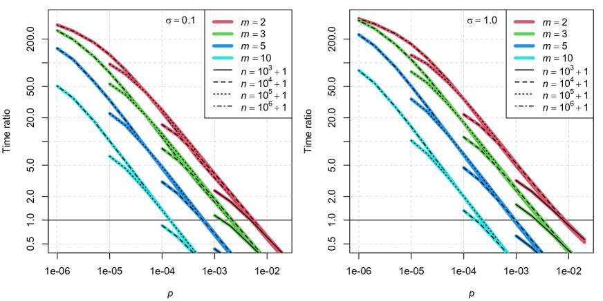
Figure 4: Median time ratio $T^{\mathrm{V}}/T^{\mathrm{Q}}$ against exit probability $p$.

Since QATS and Viterbi have respective computational complexities ${\cal O}(sm^{3}\log n)$, which on average is ${\cal O}(pm^{3}n\log n)$ by A.5, and ${\cal O}(m^{2}n)$, we expect the ratio $T^{\mathrm{V}}/T^{\mathrm{Q}}$ to behave like $(pm\log n)^{-1}$. Figure 4 shows plots of time ratios $T^{\mathrm{V}}/T^{\mathrm{Q}}$ against exit probabilities $p=p(n,s)$ with log-scales in both variables. On those plots, we observe an almost negative linear relationship between the log-ratio and the log-probability. Furthermore, for fixed $p$, the time ratio increases if either $m$ or $n$ decreases. Those plots also show that the value of the standard deviation $\sigma$ has very little impact on estimation time.

When $m=2$, accelerations of about $30$ units are possible when $p=10^{-4}$. When $n=10^{6}+1$, it means that QATS is about $30$ times faster than Viterbi when the expected number of segments is $101$, and about $140$ times faster when the expected number of segments is $11$. If $m=3$, $5$ or $10$, those ratios are smaller than for $m=2$, but still often larger than $2$, even for rather large values of $p$. When $m=10$ and $n=10^{6}+1$ for instance, QATS is about $10$ times faster than Viterbi for an expected number of segments of $11$. This shows that QATS is indeed substantially faster than Viterbi for low number of segments/change points. Note furthermore that the time ratio should be even larger for even longer sequences of observations.

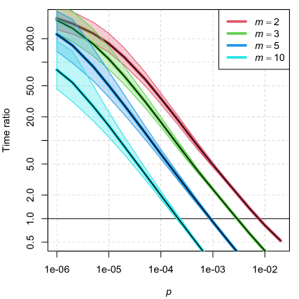
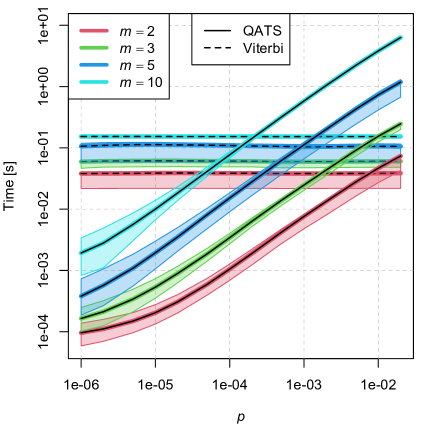
Figure 5: Median quantile time ratio $T^{\mathrm{V}}/T^{\mathrm{Q}}$ (left), and times $T^{\mathrm{Q}}$ and $T^{\mathrm{V}}$ (right) against exit probability $p$, along with $10\%$- and $90$%-quantile curves, for the setting $\sigma=1.0$ and $n=10^{6}+1$.

Figure 5 provides an assessment of the spread of time ratios and times as $p$ varies thanks to the addition of $10\%$- and $90$%-quantile curves for the setting $\sigma=1.0$ and $n=10^{6}+1$. They provide information on the expected variability around the median. The plot on the right demonstrate that the computation time of Viterbi is indeed independent of $p$ (or the expected number of segments), whereas the log-computation time of QATS depends linearly on $\log p$, except for small values of $p$.

Estimation quality.

In order to evaluate the quality of an estimate $\widehat{\boldsymbol{x}}$, we compare it with the ground truth $\boldsymbol{x}^{o}$, which denotes the true hidden path. The latter can indeed be accessed for this simulation study since data are generated. The comparison is done in terms of $\ell^{w}$-type distances between $\widehat{\boldsymbol{x}}$ and $\boldsymbol{x}^{o}$. Precisely, if $\widehat{\boldsymbol{x}}$ and $\boldsymbol{x}^{o}$ are of length $n$, we define

$$d_{w}(\widehat{\boldsymbol{x}},\boldsymbol{x}^{o})\ :=\ \begin{cases}\frac{1}{n}\sum_{k\in 1{:}n}1_{\widehat{x}_{k}\neq x_{k}^{o}}&\text{if}\ w=0,\\ \left(\frac{1}{n}\sum_{k\in 1{:}n}|\widehat{x}_{k}-x_{k}^{o}|^{w}\right)^{1/w}&\text{if}\ w>0.\end{cases}$$

Hence, the quantity $d_{0}(\widehat{\boldsymbol{x}},\boldsymbol{x}^{o})$ corresponds to the proportion of misclassified (or misestimated) states, or simply misclassification rate. On the other hand, $d_{w}(\widehat{\boldsymbol{x}},\boldsymbol{x}^{o})$ for $w>0$ gives a measure of the amplitude of misclassifications scaled to the vector length. For $w=2$, this is simply the root mean squared error. When $w=1$, it corresponds to the mean absolute error, and because $\widehat{\boldsymbol{x}}$ and $\boldsymbol{x}^{o}$ are generally close to one another, this metric is comparable to the misclassification rate.

Our simulations showed that, for the present simulations, $d_{0}$ and $d_{1}$ provide similar information on estimation error, whereas $d_{2}$ naturally puts more wait on large departure from the truth. Consequently, for each setting $(n,m,s,\sigma)$, we compute sample $\beta$-quantiles of

$$d_{w}(\widehat{\boldsymbol{x}}^{\mathrm{Q}},\boldsymbol{x}^{o}),\quad d_{w}(\widehat{\boldsymbol{x}}^{\mathrm{V}},\boldsymbol{x}^{o}),\quad\text{and}\quad d_{w}(\widehat{\boldsymbol{x}}^{\mathrm{Q}},\boldsymbol{x}^{o})-d_{w}(\widehat{\boldsymbol{x}}^{\mathrm{V}},\boldsymbol{x}^{o}),$$

for $\beta\in\{0.1,0.5,0.9\}$ and $w\in\{0,2\}$, where $\widehat{\boldsymbol{x}}^{\mathrm{Q}}$ and $\widehat{\boldsymbol{x}}^{\mathrm{V}}$ correspond to QATS and Viterbi paths, respectively. Those sample quantiles are computed from the same samples as for the computation time study.

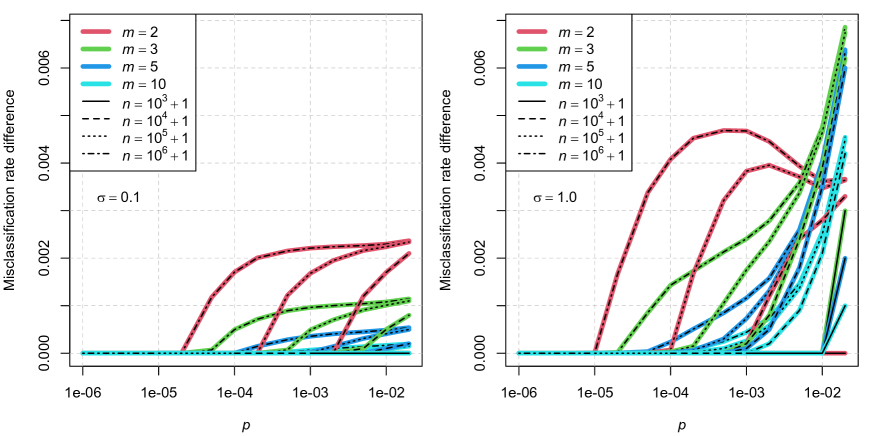
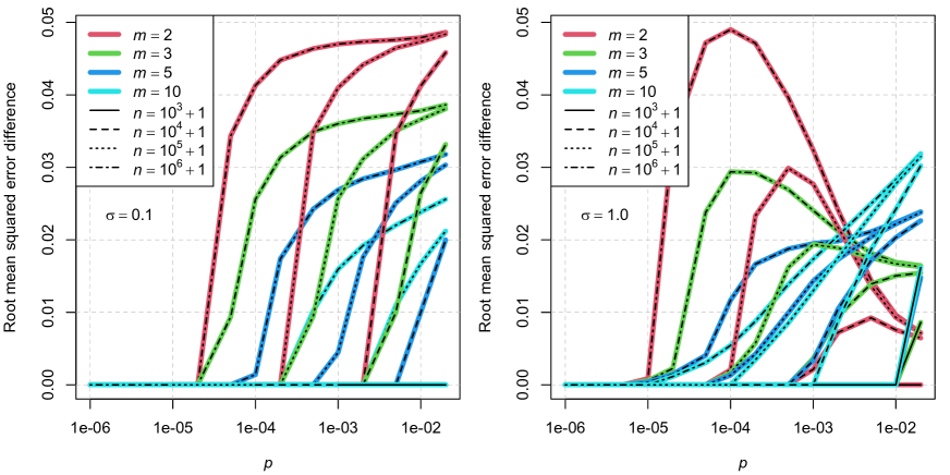
Figure 6: Difference in misclassification rates ($w=0$, top) and root mean squared error ($w=2$, bottom) against exit probability $p$ for the setting $\sigma=0.1$ (left) and $\sigma=1.0$ (right).

Figure 6 displays median error differences. Decreasing $n$, $m$ or $\sigma$ has the effect of decreasing the difference in misclassification rates between QATS and Viterbi ($w=0$, top row of plots). When $\sigma=0.1$, decreasing $p$ (or $s$) also decreases the difference, but when $\sigma=1.0$, this is no longer always true. The reason for this behavior is due to the fact that the misclassification rate for Viterbi is very low when $\sigma=0.1$, so that the main contribution in error difference is due to QATS, see also first column of Figure 7. When $\sigma=1.0$, Viterbi’s misclassification rate is no longer $0$, and actually presents a behavior similar to that of QATS’ misclassification rate, only with less variability around the median, as observed in the first column of Figure 8.

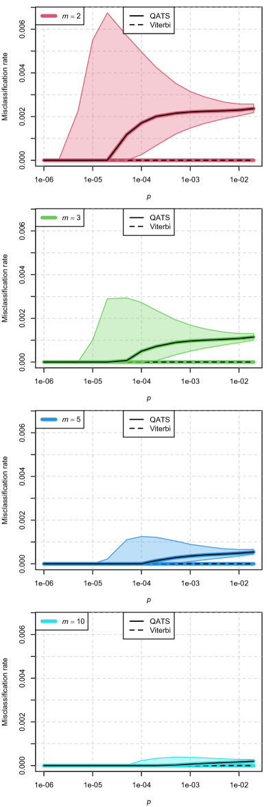
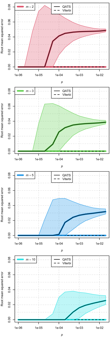
Figure 7: Misclassification rate ($w=0$, left column) and root mean squared error ($w=2$, right column) against exit probability $p$, for $m\in\{2,3,5,10\}$ (top to bottom), in the setting $\sigma=0.1$ and $n=10^{6}+1$.

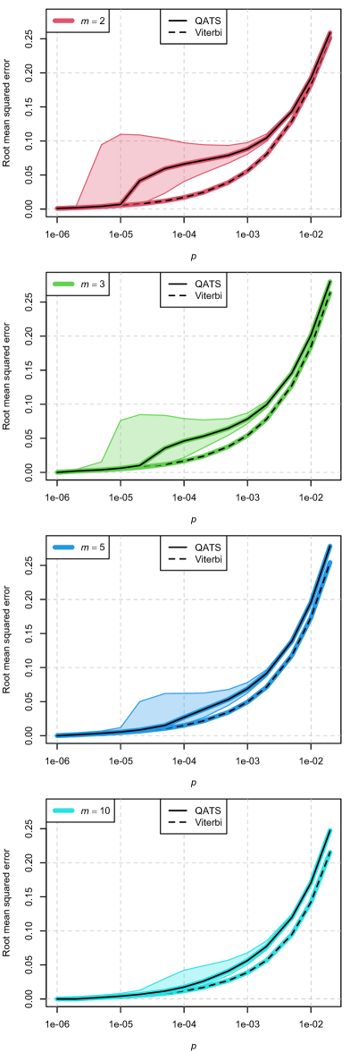
Figure 8: Misclassification rate ($w=0$, left column) and root mean squared error ($w=2$, right column) against exit probability $p$, for $m\in\{2,3,5,10\}$ (top to bottom), in the setting $\sigma=1.0$ and $n=10^{6}+1$.

Interestingly, QATS’ and Viterbi’s number of misestimated states differ by less than $0.7\%$ (in median), no matter the setting considered. This allows us to conclude that QATS and Viterbi have comparable misclassification rates.

When studying Figures 6–8 for root mean squared error ($w=2$) and differences thereof, one observes again that decreasing $n$, $m$ or $\sigma$ has the general effect of decreasing the difference in root mean squared error between QATS and Viterbi. The reason why the error difference decreases as $p$ decreases holds when $\sigma=0.1$ but not when $\sigma=1.0$ are the same as for the study of misclassification rate. When $m=2$, $\sigma=1.0$ and $p$ increases, the error difference first increases and then decreases. This is due to the fact that the variability in root mean squared error for QATS is maximal for values of $p$ in the middle of those studied.

The second column of Figure 8 displays an interesting aspect about the root mean squared error of QATS (also present for the misclassification rate, but with less amplitude) for $m\in 2{:}3$ mainly. For values of $p$ smaller than $10^{-5}$, both QATS and Viterbi present rather small errors, with more variability for QATS. Then, for values of $p$ in the interval $[10^{-5},10^{-3}]$, the error of Viterbi gradually increases, whereas that of QATS takes a larger step before flattening again. In this region, QATS is less able to differentiate between true variability (i.e. due to a large $\sigma$) and variability due to a large number of segments (i.e. a large $p$), than Viterbi. When $p$ exceeds $2\cdot 10^{-3}$, both methods interpret larger numbers of segments as extra noise in the data, so the increase in root mean squared error of QATS and Viterbi have similar behaviors again.

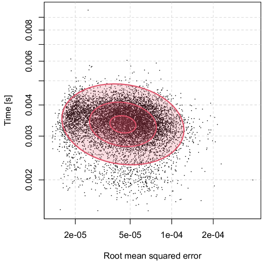
Figure 9: Computation time of QATS $T^{\mathrm{Q}}$ against root mean squared error ($w=2$), in the setting $n=10^{6}+1$, $m=3$, $p=10^{-4}$ and $\sigma=1.0$. The bivariate normal $\{10,50,90\}$-% confidence ellipses (in red) are computed on the log-scale for both the error and the time, and serve as indicators for the distribution of the data.

Time and error study.

One may think that fast computation times of QATS may sometimes be due to an error which would skip a substantial amount of steps in the procedure, but as indicated by Figure 9, this is not the case. Indeed, when plotting each of the $n_{\mathrm{sim}}$ measurements of log-time against log-root mean squared error in the setting $n=10^{6}+1$, $m=3$, $p=10^{-4}$ and $\sigma=1.0$, the two variables appear to be independent.

Robustness.

A brief robustness study involving $t$-distributed errors showed, as expected, that Viterbi is no more robust than QATS. The reason behind that is that both methods share the same input, namely the (log-)density evaluated at the observations, and both attempt to maximize a variant of likelihood.

Appendix A Proofs and technical details

A.1 Proof of Lemma 2.2

The assumption on $V$ implies immediately that all of its two-dimensional local maxima lie on the $s\times s$ grid ${\cal K}\times{\cal K}$. Further, by 2.1, the alternation of OS arrives somewhere on this grid after at most two searches, and remains on the grid afterwards. If the alternating procedure stops at a point, this point is a two dimensional local maximum of $V$, since it is a vertical and a horizontal maximum of $V$. Otherwise, by 2.1, the alternating procedure moves always to a point with a strictly larger value of $V$, implying that no loop (containing more than one point) can occur in the alternating procedure and that a chain of alternation has length at most $s(s+1)/2$. The assertion of the Lemma follows, since each search requires at most ${\cal O}\bigl{(}\log(r-\ell)\bigr{)}$ probes of $V$. ∎

A.2 An alternative version of Algorithm 3

The local maxima of ${\cal H}^{3}$ at the boundary of ${\cal K}^{3}_{\ell{:}r}$ correspond to the local maxima of ${\cal H}^{2}$ on ${\cal K}^{2}_{\ell{:}r}$. Thus, it is more interesting to find local maxima of ${\cal H}^{3}$ in the interior of ${\cal K}^{3}_{\ell{:}r}$. To this end, instead of maximizing ${\cal H}^{3}$, ${\cal K}^{2}_{\ell:(k_{2}-1)}\ni k\mapsto{\cal H}^{3}(k,k_{2})$ and ${\cal K}^{2}_{k_{1}:r}\ni k\mapsto{\cal H}^{3}(k_{1},k)$, it may be desirable to rotate each score so that their value on both ends of their respective domains coincides. Precisely, we would set

$$\bar{{\cal H}}^{2}(k)\ :=\ {\cal H}^{2}(k)-\bigl{(}{\cal H}^{2}(r)-{\cal H}^{2}(\ell+1)\bigr{)}\frac{k-\ell-1}{r-\ell-1}, k\in{\cal K}^{2}_{\ell:r},$$

$$\bar{{\cal H}}^{3}(k,k_{2})\ :=\ {\cal H}^{3}(k,k_{2})-\bigl{(}{\cal H}^{3}(k_{2}-1,k_{2})-{\cal H}^{3}(\ell+1,k_{2})\bigr{)}\frac{k-\ell-1}{k_{2}-\ell-2}, k\in{\cal K}^{3}_{\ell:(k_{2}-1)},$$

$$\bar{{\cal H}}^{3}(k_{1},k)\ :=\ {\cal H}^{3}(k_{1},k)-\bigl{(}{\cal H}^{3}(k_{1},r)-{\cal H}^{3}(k_{1},k_{1}+1)\bigr{)}\frac{k-k_{1}-1}{r-k_{1}-1}, k\in{\cal K}^{3}_{k_{1}:r},$$

whenever the above fractions are respectively well-defined, that is whenever the sets ${\cal K}^{2}_{\ell:r}$, ${\cal K}^{3}_{\ell:(k_{2}-1)}$ and ${\cal K}^{3}_{k_{1}:r}$ are respectively non-empty. Then, one would replace $H^{2}$ by $\bar{{\cal H}}^{2}$ in Algorithm 2, $H^{3}(k_{1}^{*},\cdot)$ and $H^{3}(\cdot,k_{2}^{*})$ by $\bar{{\cal H}}^{3}(k_{1}^{*},\cdot)$ and $\bar{{\cal H}}^{3}(\cdot,k_{2}^{*})$ in Algorithm 3.

A.3 Log-local likelihoods

We may define

$${\cal G}_{\ell:r}(i|x_{0})\ := \ G_{i,r}-1_{[\ell>1]}G_{i,\ell-1}$$

$$\ +1_{[\ell=1]}\log\pi_{i}+1_{[\ell>1]}q_{x_{0}i}+q_{ii}(r-\ell),$$

$${\cal G}_{\ell:k:r}(\boldsymbol{i}|x_{0})\ := \ G_{i_{1},k-1}-1_{[\ell>1]}G_{i_{1},\ell-1}+G_{i_{2},r}-G_{i_{2},k-1}$$

$$\ +1_{[\ell=1]}\log\pi_{i_{1}}+1_{[\ell>1]}q_{x_{0}i_{1}}+q_{i_{1}i_{1}}(k-\ell-1)$$

$$\ +q_{i_{1}i_{2}}+q_{i_{2}i_{2}}(r-k),$$

$${\cal G}_{\ell:k_{1}:k_{2}:r}(\boldsymbol{i}|x_{0})\ := \ G_{i_{1},k_{1}-1}-1_{[\ell>1]}G_{i_{1},\ell-1}+G_{i_{2},k_{2}-1}-G_{i_{2},k_{1}-1}+G_{i_{3},r}-G_{i_{3},k_{2}-1}$$

$$\ +1_{[\ell=1]}\log\pi_{i_{1}}+1_{[\ell>1]}q_{x_{0}i_{1}}+q_{i_{1}i_{1}}(k_{1}-\ell-1)$$

$$\ +q_{i_{1}i_{2}}+q_{i_{2}i_{2}}(k_{2}-k_{1}-1)+q_{i_{2}i_{3}}+q_{i_{3}i_{3}}(r-k_{2}),$$

so that

$$\log\Lambda_{\ell:r}(\boldsymbol{x}_{\ell:r}(i)|x_{0})\ =\ {\cal G}_{\ell:r}(i|x_{0}),$$

$$\log\Lambda_{\ell:r}(\boldsymbol{x}_{\ell:k:r}(\boldsymbol{i})|x_{0})\ =\ {\cal G}_{\ell:k:r}(\boldsymbol{i}|x_{0}),$$

$$\log\Lambda_{\ell:r}(\boldsymbol{x}_{\ell:k_{1}:k_{2}:r}(\boldsymbol{i})|x_{0})\ =\ {\cal G}_{\ell:k_{1}:k_{2}:r}(\boldsymbol{i}|x_{0}).$$

A.4 Proofs for Section 3.1

We progressively build the theory to prove 3.3. To this end, we suppose that 2 holds for the remainder of the appendix, and define the following constants:

$$\beta^{c}_{1}\ :=\ -\log 2+(n-c)\log(1-\varepsilon)+(c-1)\log\varepsilon+n\beta_{1}+\frac{n}{2}\beta_{2},\quad c\in 1{:}3,$$

as well as the following elements:

$$\psi^{1}\ :=\ \sum_{t=1}^{n}1_{[y_{t}=1]},$$

$$\psi^{2}(k)\ :=\ \sum_{t=1}^{k-1}1_{[y_{t}=1]}+\sum_{t=k}^{n}1_{[y_{t}=2]}, \text{for}\ k\in{\cal K}^{2},$$

$$\psi^{3}(\boldsymbol{k})\ :=\ \sum_{t=1}^{k_{1}-1}1_{[y_{t}=1]}+\sum_{t=k_{1}}^{k_{2}-1}1_{[y_{t}=2]}+\sum_{t=k_{2}}^{n}1_{[y_{t}=1]}, \text{for}\ \boldsymbol{k}\in{\cal K}^{3}.$$

Lemma A.1.

We have that

$${\cal H}^{c}\ =\ \beta_{1}^{c}+\beta_{2}\Bigl{(}\max\bigl{(}\psi^{c},n-\psi^{c}\bigr{)}-\frac{n}{2}\Bigr{)}\ =\ \beta_{1}^{c}+\beta_{2}\left|\psi^{c}-\frac{n}{2}\right|,\qquad c\in 1{:}3.$$

Furthermore, for each segment ${\cal K}^{2}_{a}:=(\kappa_{a-1}{:}\kappa_{a})\cap{\cal K}^{2}$, $a\in 1{:}s^{o}$, there exists $\gamma_{a}\in\mathbb{Z}/2$ such that

$${\cal H}^{2}(k)\ =\ \beta_{1}^{2}+\beta_{2}\left|k-\gamma_{a}\right|,\qquad k\in{\cal K}^{2}_{a}.$$

Likewise, for each nonempty set of contiguous index pairs ${\cal K}^{3}_{ab}:=\bigl{(}(\kappa_{a-1}{:}\kappa_{a})\times(\kappa_{b-1}{:}\kappa_{b})\bigr{)}\cap{\cal K}^{3}$, where $a,b\in 1{:}s^{o}$, $a\leq b$, there exists $\gamma_{ab}\in\mathbb{Z}/2$ such that

$${\cal H}^{3}(\boldsymbol{k})\ =\ \beta_{1}^{3}+\beta_{2}\left|k_{2}-(-1)^{a+b}k_{1}-\gamma_{ab}\right|,\qquad\boldsymbol{k}\in{\cal K}^{3}_{ab}.$$

Proof of A.1.

The special forms of $g_{i}$ and the fact that $m=2$ imply that

$${\cal G}_{1:n}(i)\ =\ \beta_{1}^{1}-\frac{n}{2}\beta_{2}+\beta_{2}\cdot\begin{cases}\psi^{1}&\text{if}\ i=1,\\ n-\psi^{1}&\text{if}\ i=2,\end{cases}$$

$${\cal G}_{1:k:n}(\boldsymbol{i})\ =\ \beta_{1}^{2}-\frac{n}{2}\beta_{2}+\beta_{2}\cdot\begin{cases}\psi^{2}(k)&\text{if}\ \boldsymbol{i}=(1,2),\\ n-\psi^{2}(k)&\text{if}\ \boldsymbol{i}=(2,1),\end{cases}$$

$${\cal G}_{1:k_{1}:k_{2}:n}(\boldsymbol{i})\ =\ \beta_{1}^{3}-\frac{n}{2}\beta_{2}+\beta_{2}\cdot\begin{cases}\psi^{3}(\boldsymbol{k})&\text{if}\ \boldsymbol{i}=(1,2,1),\\ n-\psi^{3}(\boldsymbol{k})&\text{if}\ \boldsymbol{i}=(2,1,2),\end{cases}$$ (A.1)

for $k\in{\cal K}^{2}$ and $\boldsymbol{k}\in{\cal K}^{3}$. In consequence, we find that

$${\cal H}^{c}\ =\ \beta_{1}^{c}+\beta_{2}\left(\max(\psi^{c},n-\psi^{c})-\frac{n}{2}\right)\ =\ \beta_{1}^{c}+\beta_{2}\left|\psi^{c}-\frac{n}{2}\right|,\qquad c\in 1{:}3,$$

where we used the fact that $2\max(\xi_{1},\xi_{2})=\xi_{1}+\xi_{2}+|\xi_{1}-\xi_{2}|$ in the last equality.

For the rest of the proof, observe first that for $a\in 1{:}s^{o}$ and $t\in\kappa_{a-1}{:}(\kappa_{a}-1)$, we have

$$y_{t}\ =\ \begin{cases}1&\text{if}\ y_{1}+a\ \text{is even},\\ 2&\text{if}\ y_{1}+a\ \text{is odd}.\\ \end{cases}$$

For $a\in 1{:}s^{o}$ and $k\in{\cal K}^{2}_{a}$, there exists some $\alpha_{a}\in\mathbb{Z}$ such that

$$\psi^{2}(k)\ = \ \sum_{t=1}^{n}1_{[y_{t}=1]}+1_{[k<\kappa_{a}]}\sum_{t=k}^{\kappa_{a}-1}(-1)^{y_{t}}+1_{[a<s^{o}]}\sum_{t=\kappa_{a}}^{n}(-1)^{y_{t}}$$

$$\ = \ \alpha_{a}-(-1)^{y_{1}+a}(\kappa_{a}-k).$$

Since $\gamma_{a}:=-\kappa_{a}+(-1)^{y_{1}+a}(\alpha_{a}-n/2)$ satisfies $|\psi^{2}(k)-n/2|=|k-\gamma_{a}|$, the second part of the Lemma is proved.

Let $a,b\in 1{:}s^{o}$, $a\leq b$, such that ${\cal K}^{3}_{ab}\neq\emptyset$, and fix $\boldsymbol{k}\in{\cal K}^{3}_{ab}$. In case $a=b$, then $a+b$ is even and $\kappa_{b-1}\leq k_{1}\leq k_{2}-1<\kappa_{b}$, so for some for some $\alpha_{ab}\in\mathbb{N}$ we have that

$$\psi^{3}(\boldsymbol{k})\ = \ \sum_{t=1}^{n}1_{[y_{t}=1]}-(-1)^{y_{1}+b}(k_{2}-k_{1})$$

$$\ = \ \alpha_{ab}-(-1)^{y_{1}+b}\bigl{(}k_{2}-(-1)^{a+b}k_{1}\bigr{)}.$$

When $a<b$, we have $\kappa_{a-1}\leq k_{1}\leq\kappa_{a}\leq\kappa_{b-1}\leq k_{2}\leq\kappa_{b}$ and for some $\alpha_{ab}\in\mathbb{Z}$ it holds that

$$\psi^{3}(\boldsymbol{k})\ = \ \sum_{t=1}^{n}1_{[y_{t}=1]}+1_{[k_{1}<\kappa_{a}]}\sum_{t=k_{1}}^{\kappa_{a}-1}(-1)^{y_{t}}+1_{[a+1<b]}\sum_{t=\kappa_{a}}^{\kappa_{b-1}-1}(-1)^{y_{t}}+1_{[\kappa_{b-1}<k_{2}]}\sum_{t=\kappa_{b-1}}^{k_{2}-1}(-1)^{y_{t}}$$

$$\ = \ \sum_{t=1}^{n}1_{[y_{t}=1]}-(-1)^{y_{1}+a}(\kappa_{a}-k_{1})+1_{[a+1<b]}\sum_{t=\kappa_{a}}^{\kappa_{b-1}-1}(-1)^{y_{t}}-(-1)^{y_{1}+b}(k_{2}-\kappa_{b-1})$$

$$\ = \ \alpha_{ab}-(-1)^{y_{1}+b}\bigl{(}k_{2}-(-1)^{a+b}k_{1}\bigr{)}.$$

In both cases, $\gamma_{ab}:=(-1)^{y_{1}+b}(\alpha_{ab}-n/2)$ satisfies $|\psi^{3}(\boldsymbol{k})-n/2|=|k_{2}-(-1)^{a+b}k_{1}-\gamma_{ab}|$ and thus the last part of the Lemma is proved. ∎

Proof of 3.3.

Part (i). A local maximum of ${\cal H}^{2}$ on ${\cal K}^{2}$ belonging to a set ${\cal K}^{2}_{a}$, $a\in 1{:}s^{o}$, necessarily has to be a local maximum of ${\cal H}^{2}$ restricted to that ${\cal K}^{2}_{a}$. But the structure of ${\cal H}^{2}$ and the fact that $\beta_{2}>0$ imply that local maxima of ${\cal H}^{2}$ restricted to ${\cal K}^{2}_{a}$ can only be located at its endpoints $\max(2,\kappa_{a-1})$ and $\min(\kappa_{a},n)$.

Likewise, a local maximum of ${\cal H}^{3}$ on ${\cal K}^{3}$ belonging to a set ${\cal K}^{3}_{ab}$, $a,b\in 1{:}s^{o}$ and $a\leq b$, necessarily has to be a local maximum of ${\cal H}^{3}$ restricted to that ${\cal K}^{3}_{ab}$. The structure of ${\cal H}^{3}$ and the fact that $\beta_{2}>0$ imply that local maxima of ${\cal H}^{3}$ restricted to ${\cal K}^{3}_{ab}$ are necessarily distributed as follows:

If $a+b$ is even, then ${\cal H}^{3}(\boldsymbol{k})=\beta^{3}_{1}+\beta_{2}|k_{2}-k_{1}-\gamma_{ab}|$ on ${\cal K}^{3}_{ab}$. When $a=b$, local maxima of ${\cal H}^{3}$ restricted to ${\cal K}^{3}_{ab}$ can only be located on the diagonal ${\cal K}^{3}_{ab}\cap\{\boldsymbol{k}\in{\cal K}^{3}:k_{2}=k_{1}+1\}$ or at $\bigl{(}\max(2,\kappa_{a-1}),\min(\kappa_{b},n)\bigr{)}$. When $a<b$, then $a<b-1$ (because $a+b$ is even) and only $\bigl{(}\max(2,\kappa_{a-1}),\min(\kappa_{b},n)\bigr{)}$ or $\bigl{(}\kappa_{a},\kappa_{b-1}\bigr{)}$ are potential local maxima of ${\cal H}^{3}$ restricted to ${\cal K}^{3}_{ab}$.

If $a+b$ is odd, then $a<b$ and ${\cal H}^{3}(\boldsymbol{k})=\beta^{3}_{1}+\beta_{2}|k_{2}+k_{1}-\gamma_{ab}|$ on ${\cal K}^{3}_{ab}$. That means, local maxima of ${\cal H}^{3}$ restricted to ${\cal K}^{3}_{ab}$ can only be located at $\bigl{(}\max(2,\kappa_{a-1}),\kappa_{b-1}\bigr{)}$ or $\bigl{(}\kappa_{a},\min(\kappa_{b},n)\bigr{)}$.

All in all, the sum of indices indexing local maxima of ${\cal H}^{3}$ in the interior of ${\cal K}^{3}$ is always odd.

Part (ii). Let $a\in 1{:}(s^{o}-1)$ be arbitrary. We suppose without loss of generality that $y_{\kappa_{a}}=1$. It is then clear to see that

$$\psi^{3}(\kappa_{a-1},\kappa_{a})\ =\ \psi^{3}(\kappa_{a},\kappa_{a+1})+(\kappa_{a+1}-\kappa_{a-1}).$$ (A.2)

It further holds that $2\psi^{3}(\kappa_{a-1},\kappa_{a})\geq n+2$ or $2\psi^{3}(\kappa_{a},\kappa_{a+1})\leq n-2$, because otherwise the relation in (A.2) implies that $\kappa_{a+1}-\kappa_{a-1}<2$, which is a contradiction.

• In case that $2\psi^{3}(\kappa_{a-1},\kappa_{a})\geq n+2$, we apply (A.1) and obtain

  $${\cal H}^{3}(k_{1},k_{2})\ =\ {\cal G}_{1:k_{1}:k_{2}:n}(1,2,1)\ \geq\ {\cal G}_{1:k_{1}:k_{2}:n}(2,1,2)$$

  for $(k_{1},k_{2})\in{\cal K}^{3}$ and $\|(k_{1},k_{2})-(\kappa_{a-1},\kappa_{a})\|_{1}\leq 1$. Thus, the pair $(\kappa_{a-1},\kappa_{a})$ is a local maximum of ${\cal H}^{3}$.

• In case that $2\psi^{3}(\kappa_{a},\kappa_{a+1})\leq n-2$, similarly as above, by (A.1) we obtain

  $${\cal H}^{3}(k_{1},k_{2})\ =\ {\cal G}_{1:k_{1}:k_{2}:n}(2,1,2)\ \geq\ {\cal G}_{1:k_{1}:k_{2}:n}(1,2,1)$$

  for $(k_{1},k_{2})\in{\cal K}^{3}$ and $\|(k_{1},k_{2})-(\kappa_{a},\kappa_{a+1})\|_{1}\leq 1$. Thus, the pair $(\kappa_{a},\kappa_{a+1})$ is a local maximum of ${\cal H}^{3}$.

Recall that at least one of the two above cases is valid, which concludes the proof. ∎

Remark A.2.

The intuition behind the fact that $a+b$ must be odd could be given as follows: The search for the best local path with three segments looks for bumps, that is a state sequence $(1,2,1)$ or $(2,1,2)$ with jumps occurring at some $2\leq\kappa_{a}<\kappa_{b}\leq n$. But for such a feature to exist in $\boldsymbol{x}^{o}$, it is necessary for $a$ and $b$ to not share the same parity, i.e. $a+b$ must be odd.

A.5 Proofs for Section 3.2

We start with some technical preparations. Recall that $\kappa_{s^{o}}=n+1$ and define, when $s^{o}\geq 2$, the numbers $w(a)_{1},\ldots,w(a)_{s^{o}-1}$ to be the sorted elements of $(1{:}s^{o})\setminus\{a\}$ and when $s^{o}\geq 3$, the numbers $w(a,b)_{1},\ldots,w(a,b)_{s^{o}-2}$ to be those of $(1{:}s^{o})\setminus\{a,b\}$. Furthermore, we let

$$\varphi^{c}\ :=\ \left\lceil\frac{s^{o}-c}{2}\right\rceil\qquad\text{for}\ c\in 1{:}3,$$

and set to $0$ any sum whose index of summation ranges from $1$ to $0$.

Lemma A.3.

If $s^{o}\geq 1$, we have that

$${\cal H}^{1}\ =\ \beta_{1}^{1}+\beta_{2}\left|\frac{n}{2}-\eta^{1}\right|\qquad\text{with}\ \eta^{1}\ :=\ \sum_{t=1}^{\varphi^{1}}\left(\kappa_{2t}-\kappa_{2t-1}\right).$$

If $s^{o}\geq 2$ and $a\in 1{:}(s^{o}-1)$, then

$${\cal H}^{2}(\kappa_{a})\ =\ \beta_{1}^{2}+\beta_{2}\left|\frac{n}{2}-\eta^{2}(a)\right|\qquad\text{with}\ \eta^{2}(a)\ :=\ \sum_{t=1}^{\varphi^{2}}\left(\kappa_{w(a)_{2t}}-\kappa_{w(a)_{2t-1}}\right).$$

If $s^{o}\geq 3$ and $a,b\in 1{:}(s^{o}-1)$, $a<b$ and $a+b$ odd, then

$${\cal H}^{3}(\kappa_{a},\kappa_{b})\ =\ \beta_{1}^{3}+\beta_{2}\left|\frac{n}{2}-\eta^{3}(a,b)\right|\qquad\text{with}\ \eta^{3}(a,b)\ :=\ \sum_{t=1}^{\varphi^{3}}\left(\kappa_{w(a,b)_{2t}}-\kappa_{w(a,b)_{2t-1}}\right).$$

Proof of A.3.

Since $|\psi^{c}-n/2|=|(n-\psi^{c})-n/2|$ for all arguments of $\psi^{c}$ and all $c\in 1{:}3$, we may assume, without loss of generality, that $y_{1}=1$. Hence, $y_{t}$ is equal to $2$ on $\kappa_{2t-1}{:}(\kappa_{2t}-1)$, for all $t\in 1{:}\varphi^{1}$ (when $s^{o}>1$, otherwise $\varphi^{1}=0$ and $y_{t}$ is always $1$). Thus $\psi^{1}=n-\eta^{1}$.

For the results concerning ${\cal H}^{2}$ and ${\cal H}^{3}$, we distinguish between the four cases generated by the various combinations of $s^{o}$ even or odd and $a$ even or odd (and therefore $b$ odd or even). We only prove the result concerning $s^{o}$ odd and $a$ even. The proof of the other three cases is analogous.

When $s^{o}\geq 2$ is odd and $a\in 1{:}(s^{o}-1)$ is even, we have

$$\psi^{2}(\kappa_{a})\ = \ (\kappa_{1}-1)+\cdots+(\kappa_{a-1}-\kappa_{a-2})+(\kappa_{a+2}-\kappa_{a+1})+\cdots+(\kappa_{s^{o}-1}-\kappa_{s^{o}-2})$$

$$\ = \ -(\kappa_{2}-\kappa_{1})-\cdots-(\kappa_{a-2}-\kappa_{a-3})-(\kappa_{a+1}-\kappa_{a-1})$$

$$\ -(\kappa_{a+3}-\kappa_{a+2})-\cdots-(\kappa_{s^{o}}-\kappa_{s^{o}-1})+n$$

$$\ = \ n-\eta^{2}(a).$$

When $s^{o}\geq 3$ is odd and $a,b\in 1{:}(s^{o}-1)$ with $a<b$, $a$ even and $b$ odd, we have

$$\psi^{3}(\kappa_{a},\kappa_{b})\ = \ (\kappa_{1}-1)+\cdots+(\kappa_{a-1}-\kappa_{a-2})$$

$$\ +(\kappa_{a+2}-\kappa_{a+1})+\cdots+(\kappa_{b-1}-\kappa_{b-2})$$

$$\ +(\kappa_{b+2}-\kappa_{b+1})+\cdots+(\kappa_{s^{o}-2}-\kappa_{s^{o}-3})+(n-\kappa_{s^{o}-1}+1)$$

$$\ = \ -(\kappa_{2}-\kappa_{1})-\cdots-(\kappa_{a-2}-\kappa_{a-3})-(\kappa_{a+1}-\kappa_{a-1})$$

$$\ -(\kappa_{a+3}-\kappa_{a+2})-\cdots-(\kappa_{b-2}-\kappa_{b-3})-(\kappa_{b+1}-\kappa_{b-1})$$

$$\ -(\kappa_{b+3}-\kappa_{b+2})-\cdots-(\kappa_{s^{o}-1}-\kappa_{s^{o}-2})+n$$

$$\ = \ n-\eta^{3}(a,b).\qed$$

Lemma A.4.

When $s^{o}=1$,

$${\cal H}^{1}\ =\ \beta_{1}^{1}+\beta_{2}\frac{n}{2},$$

$${\cal H}^{2}(2)\ =\ {\cal H}^{2}(n)\ =\ \beta_{1}^{2}+\beta_{2}\left(\frac{n}{2}-1\right)\ >\ {\cal H}^{2}(k),\qquad k\in{\cal K}^{2}\setminus\{2,n\}$$

$${\cal H}^{3}(k,k+1)\ =\ \beta_{1}^{3}+\beta_{2}\left(\frac{n}{2}-1\right)\ >\ {\cal H}^{3}(\boldsymbol{k}),\qquad k\in{\cal K}^{2}\setminus\{n\},\,\boldsymbol{k}\in{\cal K}^{3},k_{1}+1<k_{2}.$$

When $s^{o}=2$,

$${\cal H}^{1}\ =\ \beta_{1}^{1}+\beta_{2}\left|\frac{n}{2}-\kappa_{1}+1\right|,$$

$${\cal H}^{2}(\kappa_{1})\ =\ \beta_{1}^{2}+\beta_{2}\frac{n}{2} >\ {\cal H}^{2}(k),\qquad k\in{\cal K}^{2}\setminus\{\kappa_{1}\},$$

$${\cal H}^{3}(2,\kappa_{1})\ =\ {\cal H}^{3}(\kappa_{1},n)\ =\ \beta_{1}^{3}+\beta_{2}\left(\frac{n}{2}-1\right) >\ {\cal H}^{3}(\boldsymbol{k}),\qquad\boldsymbol{k}\in{\cal K}^{3}\setminus\{(2,\kappa_{1}),(\kappa_{1},n)\},$$

provided $(2,\kappa_{1})$ and $(\kappa_{1},n)$ are elements of ${\cal K}^{3}$, otherwise the corresponding expression is omitted.

When $s^{o}=3$ and for $a\in 1{:}2$,

$${\cal H}^{1}\ =\ \beta_{1}^{1}+\beta_{2}\left|\frac{n}{2}-\kappa_{2}+\kappa_{1}\right|,$$

$${\cal H}^{2}(\kappa_{a})\ =\ \beta_{1}^{2}+\beta_{2}\left|\frac{n}{2}-\kappa_{w(a)_{1}}+1\right| >{\cal H}^{2}(k),\qquad k\in{\cal K}^{2}\setminus\{2,\kappa_{1},\kappa_{2},n\},$$

$${\cal H}^{2}(2)\ =\ {\cal H}^{2}(n)\ =\ \beta_{1}^{2}+\beta_{2}\left|\frac{n}{2}-\kappa_{2}+\kappa_{1}-1\right| >{\cal H}^{2}(k),\qquad k\in{\cal K}^{2}\setminus\{2,\kappa_{1},\kappa_{2},n\},$$

$${\cal H}^{3}(\kappa_{1},\kappa_{2})\ =\ \beta_{1}^{3}+\beta_{2}\frac{n}{2} >{\cal H}^{3}(\boldsymbol{k}),\qquad\boldsymbol{k}\in{\cal K}^{3}\setminus\{(\kappa_{1},\kappa_{2})\}.$$

Proof of A.4.

Similarly as in the previous proof, since $|\psi^{c}-n/2|=|(n-\psi^{c})-n/2|$ for all arguments of $\psi^{c}$ and all $c\in 1{:}3$, we may assume, without loss of generality, that $y_{1}=1$ and study maxima and minima of $\psi^{c}$ to infer on maxima of $|\psi^{c}-n/2|$

When $s^{o}=1$, $\psi^{2}(k)=k-1$, so ${\cal H}^{2}(k)=\beta_{1}^{2}+\beta_{2}|n/2-k+1|$ with maximum $\beta_{1}^{2}+\beta_{2}(n/2-1)$ attained at $k=2$ and $k=n$. Likewise, $\psi^{3}(\boldsymbol{k})=n-k_{2}+k_{1}$, so ${\cal H}^{3}(\boldsymbol{k})=\beta_{1}^{3}+\beta_{2}|n/2-k_{2}+k_{1}|$ with maximum $\beta_{1}^{3}+\beta_{2}(n/2-1)$ attained at $\boldsymbol{k}\in{\cal K}^{3}$ such that $k_{1}+1=k_{2}$.

When $s^{o}=2$, $\psi^{2}$ is by definition maximal and equal to $n$ at $\kappa_{1}$, whereas its minimal value is at least as large as $2$. Likewise, $\psi^{3}$ is maximal with value $n-1$ at $(\kappa_{1},n)$ if $\kappa_{1}<n$ and minimal with values $1$ at $(2,\kappa_{1})$ if $2<\kappa_{1}$. Since $n>2$, at least one of the two cases must hold, yielding a maximum of $\beta_{1}^{3}+\beta_{2}(n/2-1)$ for ${\cal H}^{3}$.

When $s^{o}=3$, by Part (i) of 3.3, the maximum of ${\cal H}^{2}$ is attained either at the boundaries $2$ or $n$, or at the change points $\kappa_{1}$ or $\kappa_{2}$. In the first case, $\psi^{2}(2)=\kappa_{2}-\kappa_{1}+1$ and $\psi^{2}(n)=n-\kappa_{2}+\kappa_{1}-1$, yielding ${\cal H}^{2}(2)={\cal H}^{2}(n)=\beta_{1}^{2}+\beta_{2}|n/2-\kappa_{2}-\kappa_{1}-1|$, and in the second case, $\psi^{2}(\kappa_{1})=\kappa_{2}-1$ and $\psi^{2}(\kappa_{2})=\kappa_{1}-1$, yielding ${\cal H}^{2}(\kappa_{a})=\beta_{1}^{2}+\beta_{2}|n/2-\kappa_{w(a)_{1}}+1|$, for $a\in 1{:}2$. As to ${\cal H}^{3}$, we have that $\psi^{3}$ is maximal and equal to $n$ at $(\kappa_{1},\kappa_{2})$, and at least as large as $3$ otherwise. ∎

Proof of 3.4.

The proof of each inequality either derives directly from A.4 or uses parts of its results. For instance, since $\beta_{1}^{1}-\beta_{1}^{2}=\beta_{1}^{2}-\beta_{1}^{3}=\beta_{2}\delta>0$, inequalities concerning $s^{o}=1$ as well as the first inequality concerning $s^{o}=2$ are clear. Now, when $s^{o}=2$, then ${\cal H}^{2}(\kappa_{1})>{\cal H}^{1}$ holds if, and only if, $n/2-|n/2-\kappa_{1}+1|>\delta$, which is equivalent to $\kappa_{1}\in(1+\delta,n+1-\delta)$.

We now consider the case $s^{o}=3$. Then ${\cal H}^{2}(\kappa_{1})>{\cal H}^{1}$ is equivalent to

$$\left|\frac{n}{2}-\kappa_{2}+1\right|-\left|\frac{n}{2}-\kappa_{2}+\kappa_{1}\right|\ >\ \delta.$$

Now, the only possibility for the displayed inequality to hold is if $\kappa_{2}>n/2+1$, since otherwise $\kappa_{2}\leq n/2+1<n/2+\kappa_{1}$ would imply that the displayed inequality simplifies to $\kappa_{1}<1-\delta$, which is impossible. In consequence, either $\kappa_{2}\leq n/2+\kappa_{1}$, in which case the displayed inequality is equivalent to $\kappa_{1}<2\kappa_{2}-n-1-\delta$, or $\kappa_{2}>n/2+\kappa_{1}$, in which case the displayed inequality is equivalent to $\kappa_{1}>1+\delta$. Combining our findings, the displayed inequality is equivalent to $\kappa_{2}>n/2+1$ and $\kappa_{1}\in(1+\delta,2\kappa_{2}-n-1-\delta)$. To conclude, note that the latter interval is non-empty if, and only if, $\kappa_{2}>n/2+1+\delta$. The equivalence statements regarding ${\cal H}^{2}(\kappa_{2})>{\cal H}^{1}$ and ${\cal H}^{3}(\kappa_{1},\kappa_{2})>{\cal H}^{1}$ are proved with similar arguments.

We prove the equivalent statement to ${\cal H}^{3}(\kappa_{1},\kappa_{2})>\max_{k\in{\cal K}^{2}}\,{\cal H}^{2}(k)$. To this end, note that the inequality holds if, and only if, $n/2-|n/2-\kappa_{a}+1|>\delta$, $a\in 1{:}2$, and $n/2-|n/2-\kappa_{2}+\kappa_{1}-1|>\delta$. The first of those two assertions holds if, and only if, $\kappa_{a}\in(\delta+1,n+1-\delta)$ for $a\in 1{:}2$. But since $\kappa_{1}<\kappa_{2}$, the last statement is equivalent to $\delta+1<\kappa_{1}$ and $\kappa_{2}<n+1-\delta$, which imply $\kappa_{2}-\kappa_{1}<\kappa_{2}-1-\delta\leq n-1-\delta$. As to the second assertion, it holds if, and only if, $\delta-1<\kappa_{2}-\kappa_{1}<n-1-\delta$, where the second inequality was already implied by the first assertion. ∎

Proof of 3.5.

The proof of this Lemma relies on the findings of A.3. Observe first that ${\cal H}^{2}(\kappa_{a})>{\cal H}^{1}$ is equivalent to

$$\Delta\ :=\ \left|\frac{n}{2}-\eta^{2}(a)\right|-\left|\frac{n}{2}-\eta^{1}\right|\ >\ \delta.$$

Let us denote by $\boldsymbol{x}^{*}_{a}$ the path which is equal to $1$ on $1{:}(\kappa_{a}-1)$, and equals $2$ on $\kappa_{a}{:}n$. Then, if we define

$$C_{1}\ :=\ \|\boldsymbol{x}-\boldsymbol{1}\|_{1}\ =\ \|\boldsymbol{x}_{1:(\kappa_{a}-1)}-\boldsymbol{1}\|_{1}+(n-\kappa_{a}+1)-\|\boldsymbol{x}_{\kappa_{a}:n}-\boldsymbol{2}\|_{1},$$

$$C_{2}\ :=\ \|\boldsymbol{x}-\boldsymbol{x}^{*}_{a}\|_{1}\ =\ \|\boldsymbol{x}_{1:(\kappa_{a}-1)}-\boldsymbol{1}\|_{1}+\|\boldsymbol{x}_{\kappa_{a}:n}-\boldsymbol{2}\|_{1},$$

and note that $C_{1}$ is equal to $\eta^{1}$ if $x_{1}=1$, and to $n-\eta^{1}$ if $x_{1}=2$, and likewise that $C_{2}$ is equal to $\eta^{2}(a)$ if $x_{1}=1$, and to $n-\eta^{2}(a)$ if $x_{1}=2$. In consequence, we find that

$$\Delta\ =\ \left|\frac{n}{2}-C_{2}\right|-\left|\frac{n}{2}-C_{1}\right|.$$

Next, define

$$D_{1}\ :=\ \frac{1}{2}-\frac{\|\boldsymbol{x}_{1:(\kappa_{a}-1)}-\boldsymbol{1}\|_{1}}{\kappa_{a}-1}\quad\text{and}\quad D_{2}\ :=\ \frac{1}{2}-\frac{\|\boldsymbol{x}_{\kappa_{a}:n}-\boldsymbol{2}\|_{1}}{n-\kappa_{a}+1},$$

and study all four combinations $(\pm D_{1},\pm D_{2})\geq(0,0)$.

First of all, when $D_{1},D_{2}\geq 0$, we find that

$$C_{2}\ \leq\ \frac{1}{2}(\kappa_{a}-1)+\frac{1}{2}(n-\kappa_{a}+1)\ =\ \frac{n}{2}.$$

Simple calculations then show that $\Delta>\delta$ is equivalent to

$$D_{1}\ >\ \frac{1}{2}\cdot\frac{\delta}{\kappa_{a}-1}\quad\text{and}\quad D_{2}\ >\ \frac{1}{2}\cdot\frac{\delta}{n-\kappa_{a}+1}.$$

Second of all, when $D_{1},D_{2}\leq 0$, we find that

$$C_{2}\ \geq\ \frac{1}{2}(\kappa_{a}-1)+\frac{1}{2}(n-\kappa_{a}+1)\ =\ \frac{n}{2},$$

so that $\Delta>\delta$ is equivalent to

$$D_{1}\ <\ -\frac{1}{2}\cdot\frac{\delta}{\kappa_{a}-1}\quad\text{and}\quad D_{2}\ <\ -\frac{1}{2}\cdot\frac{\delta}{n-\kappa_{a}+1}.$$

Third, when $D_{1}\leq 0\leq D_{2}$, we have that

$$C_{1}\ \geq\ \frac{1}{2}(\kappa_{a}-1)+(n-\kappa_{a}+1)-\frac{1}{2}(n-\kappa_{a}+1)\ =\ \frac{n}{2}.$$

But in that case, $\Delta>\delta$ is equivalent to

$$D_{1}\ >\ \frac{1}{2}\cdot\frac{\delta}{\kappa_{a}-1}\quad\text{or}\quad D_{2}\ <\ -\frac{1}{2}\cdot\frac{\delta}{n-\kappa_{a}+1},$$

which is incompatible with the assumption that $D_{1}\leq 0\leq D_{2}$. Finally, when $D_{2}\leq 0\leq D_{1}$, we have that $C_{1}\leq n/2$, so $\Delta>\delta$ is equivalent to

$$D_{1}\ <\ -\frac{1}{2}\cdot\frac{\delta}{\kappa_{a}-1}\quad\text{or}\quad D_{2}\ >\ \frac{1}{2}\cdot\frac{\delta}{n-\kappa_{a}+1},$$

which is again incompatible with the assumption that $D_{2}\leq 0\leq D_{1}$.

In conclusion, ${\cal H}^{2}(\kappa_{a})>{\cal H}^{1}$ is equivalent to either one of the two pairs of inequalities

$$\begin{cases}\frac{\|\boldsymbol{x}_{1:(\kappa_{a}-1)}-\boldsymbol{1}\|_{1}}{\kappa_{a}-1}\ <\ \frac{1}{2}-\frac{1}{2}\cdot\frac{\delta}{\kappa_{a}-1},\\ \frac{\|\boldsymbol{x}_{\kappa_{a}:n}-\boldsymbol{2}\|_{1}}{n-\kappa_{a}+1}\ <\ \frac{1}{2}-\frac{1}{2}\cdot\frac{\delta}{n-\kappa_{a}+1},\end{cases}\quad\text{or}\qquad\begin{cases}\frac{\|\boldsymbol{x}_{1:(\kappa_{a}-1)}-\boldsymbol{1}\|_{1}}{\kappa_{a}-1}\ >\ \frac{1}{2}+\frac{1}{2}\cdot\frac{\delta}{\kappa_{a}-1},\\ \frac{\|\boldsymbol{x}_{\kappa_{a}:n}-\boldsymbol{2}\|_{1}}{n-\kappa_{a}+1}\ >\ \frac{1}{2}+\frac{1}{2}\cdot\frac{\delta}{n-\kappa_{a}+1}.\end{cases}$$

Multiplying by $-1$ and adding $1$ to the latter set of inequalities, and simplifying the left-hand sides yield the desired result. ∎

The arguments of the proof of 3.6 are essentially the same as those given in the proof of 3.5. The proof is therefore omitted.

A.6 Proof for Section 4

Lemma A.5.

Let $\boldsymbol{X}:=(X_{k})_{k=1}^{n}$ be a Markov chain with state space $1{:}m$, initial distribution $\boldsymbol{\pi}=m^{-1}\boldsymbol{1}$ and transition matrix $\boldsymbol{p}\in[0,1]^{m\times m}$ such that $\boldsymbol{p}$ is equal to $1-p(n,s)$ on the diagonal and $(m-1)^{-1}p(n,s)$ elsewhere, with exit probability $p(n,s)=(s-1)/(n-1)$. Then, the expected number of segments of $\boldsymbol{X}$ is equal to $s$.

Proof.

The expected number of segments of $\boldsymbol{X}$ is equal to

$$1+\mathop{\rm I\!E}\nolimits\left(\sum_{k=1}^{n-1}1_{[X_{k}\neq X_{k+1}]}\right)\ =\ 1+\sum_{k=1}^{n-1}\mathop{\rm I\!P}\nolimits(X_{k}\neq X_{k-1})\ =\ 1+(n-1)p(n,s)\ =\ s.\qed$$

References

-
Backurs and Tzamos (2017)
Backurs, A. and Tzamos, C. (2017).
Improving Viterbi is hard: Better runtimes imply faster clique
algorithms.
In Proceedings of the 34th International Conference on
Machine Learning (D. Precup and Y. W. Teh, eds.), vol. 70 of
Proceedings of Machine Learning Research. PMLR.
URL https://proceedings.mlr.press/v70/backurs17a.html -
Bai (1997)
Bai, J. (1997).
Estimating multiple breaks one at a time.
Econ. Theory 13 315–352.
URL https://doi.org/10.1017/S0266466600005831 -
Ball and Rice (1992)
Ball, F. G. and Rice, J. A. (1992).
Stochastic models for ion channels: Introduction and bibliography.
Math. Biosci. 112 189–206.
URL https://doi.org/10.1016/0025-5564(92)90023-p - Baum (1972) Baum, L. E. (1972). An inequality and associated maximization technique in statistical estimation for probabilistic functions of Markov processes. In Inequalities, III (Proc. Third Sympos., Univ. California, Los Angeles, Calif., 1969; dedicated to the memory of Theordore S. Motzkin).
-
Baum and Petrie (1966)
Baum, L. E. and Petrie, T. (1966).
Statistical inference for probabilistic functions of finite state
Markov chains.
Ann. Math. Statist. 37 1554–1563.
URL https://doi.org/10.1214/aoms/1177699147 -
Baum et al. (1970)
Baum, L. E., Petrie, T., Soules, G. and
Weiss, N. (1970).
A maximization technique occurring in the statistical analysis of
probabilistic functions of Markov chains.
Ann. Math. Statist. 41 164–171.
URL https://doi.org/10.1214/aoms/1177697196 -
Blelloch (1989)
Blelloch, G. E. (1989).
Scans as primitive parallel operations.
IEEE Transactions on Computers 38 1526–1538.
URL https://doi.org/10.1109/12.42122 -
Bulla et al. (2019)
Bulla, J., Langrock, R. and Maruotti, A. (2019).
Guest editor’s introduction to the special issue on “Hidden
Markov models: theory and applications”.
Metron 77 63–66.
URL https://doi.org/10.1007/s40300-019-00157-2 -
Cairo et al. (2016)
Cairo, M., Farina, G. and Rizzi, R. (2016).
Decoding hidden Markov models faster than Viterbi via online
matrix-vector (max, +)-multiplication.
In Proceedings of the Thirtieth AAAI Conference on Artificial
Intelligence (AAAI-16). Association for the Advancement of Artificial
Intelligence, The AAAI Press, Palo Alto, California.
URL https://dl.acm.org/doi/abs/10.5555/3016100.3016106 -
Cappé et al. (2005)
Cappé, O., Moulines, E. and Rydén, T.
(2005).
Inference in Hidden Markov Models.
Springer Series in Statistics, Springer, New York.
URL https://doi.org/10.1007/0-387-28982-8 -
Carvalho and Lawrence (2008)
Carvalho, L. E. and Lawrence, C. E. (2008).
Centroid estimation in discrete high-dimensional spaces with
applications in biology.
Proc. Natl. Acad. Sci. U.S.A. 105 3209–3214.
URL https://doi.org/10.1073/pnas.0712329105 -
Durbin et al. (1998)
Durbin, R., Eddy, S. R., Krogh, A. and
Mitchison, G. (1998).
Biological Sequence Analysis: Probabilistic Models of
Proteins and Nucleic Acids.
Cambridge University Press.
URL https://doi.org/10.1017/CBO9780511790492 -
Eddelbuettel (2013)
Eddelbuettel, D. (2013).
Seamless R and C++ Integration with Rcpp.
Springer, New York.
ISBN 978-1-4614-6867-7.
URL https://www.doi.org/10.1007/978-1-4614-6868-4 -
Eddelbuettel and Balamuta (2018)
Eddelbuettel, D. and Balamuta, J. J. (2018).
Extending R with C++: A brief introduction to Rcpp.
The American Statistician 72 28–36.
URL https://www.doi.org/10.1080/00031305.2017.1375990 -
Eddelbuettel and François (2011)
Eddelbuettel, D. and François, R. (2011).
Rcpp: Seamless R and C++ integration.
Journal of Statistical Software 40 1–18.
URL https://www.doi.org/10.18637/jss.v040.i08 -
Eddelbuettel and Sanderson (2014)
Eddelbuettel, D. and Sanderson, C. (2014).
RcppArmadillo: Accelerating R with high-performance C++ linear
algebra.
Computational Statistics and Data Analysis 71
1054–1063.
URL http://dx.doi.org/10.1016/j.csda.2013.02.005 -
Ephraim and Merhav (2002)
Ephraim, Y. and Merhav, N. (2002).
Hidden Markov processes.
In Special issue on Shannon theory: perspective, trends,
and applications (H. J. Landau, J. E. Mazo, S. Shamai and J. Ziv, eds.),
vol. 48, no. 6. Institute of Electrical and Electronics Engineers, Inc.
(IEEE), Piscataway, NJ, 1518–1569.
URL https://doi.org/10.1109/TIT.2002.1003838 -
Esposito and Radicioni (2009)
Esposito, R. and Radicioni, D. P. (2009).
CarpeDiem: Optimizing the Viterbi algorithm and applications to
supervised sequential learning.
J. Mach. Learn. Res. 10 1851–1880.
URL https://dl.acm.org/doi/10.5555/1577069.1755847 -
Fariselli et al. (2005)
Fariselli, P., Martelli, P. L. and Casadio, R.
(2005).
A new decoding algorithm for hidden Markov models improves the
prediction of the topology of all-beta membrane proteins.
BMC Bioinformatics 6.
URL https://doi.org/10.1186/1471-2105-6-S4-S12 -
Forney (1973)
Forney, G. D., Jr. (1973).
The Viterbi algorithm.
Proc. IEEE 61 268–278.
URL https://doi.org/10.1109/PROC.1973.9030 - Frühwirth-Schnatter (2006) Frühwirth-Schnatter, S. (2006). Finite Mixture and Markov Switching Models. Springer Series in Statistics, Springer, New York.
-
Gales and Young (2008)
Gales, M. and Young, S. (2008).
The application of hidden markov models in speech recognition.
Foundations and Trends in Signal Processing 1
195–304.
URL http://dx.doi.org/10.1561/2000000004 -
Gotoh et al. (1998)
Gotoh, Y., Hochberg, M. M. and Silverman, H. F.
(1998).
Efficient training algorithms for HMMs using incremental
estimation.
IEEE Trans. Speech Audio Processing 6 539–548.
URL https://doi.org/10.1109/89.725320 -
Hamilton (1989)
Hamilton, J. D. (1989).
A new approach to the economic analysis of nonstationary time series
and the business cycle.
Econometrica 57 357–384.
URL https://doi.org/10.2307/1912559 -
Hassan et al. (2021)
Hassan, S. S., Särkkä, S. and
García-Fernández, A. F. (2021).
Temporal parallelization of inference in hidden Markov models.
IEEE Trans. Signal Process. 69 4875–4887.
URL https://doi.org/10.1109/TSP.2021.3103338 -
Kaji et al. (2010)
Kaji, N., Fujiwara, Y., Yoshinaga, N. and
Kitsuregawa, M. (2010).
Efficient staggered decoding for sequence labeling.
In Proceedings of the 48th Annual Meeting of the Association
for Computational Linguistics. Association for Computational Linguistics,
Uppsala, Sweden.
URL https://aclanthology.org/P10-1050 -
Karplus (2009)
Karplus, K. (2009).
SAM-T08, HMM-based protein structure prediction.
Nucleic Acids Research 37 W492–W497.
URL https://doi.org/10.1093/nar/gkp403 -
Kiefer (1953)
Kiefer, J. (1953).
Sequential minimax search for a maximum.
Proc. Amer. Math. Soc. 4 502–506.
URL https://doi.org/10.2307/2032161 -
Kovács et al. (2020)
Kovács, S., Li, H., Haubner, L., Munk, A.
and Bühlmann, P. (2020).
Optimistic search strategy: Change point detection for large-scale
data via adaptive logarithmic queries.
Preprint, arXiv:2010.10194.
URL https://arxiv.org/abs/2010.10194 -
Ladner and Fischer (1980)
Ladner, R. E. and Fischer, M. J. (1980).
Parallel prefix computation.
J. Assoc. Comput. Mach. 27 831–838.
URL https://doi.org/10.1145/322217.322232 -