Gravitational waves from binary black holes in a self-interacting scalar dark matter cloud

Abstract

We investigate the imprints of accretion and dynamical friction on the gravitational-wave signals emitted by binary black holes embedded in a scalar dark matter cloud. As a key feature in this work, we focus on scalar fields with a repulsive self-interaction that balances against the self-gravity of the cloud. To a first approximation, the phase of the gravitational-wave signal receives extra correction terms at $-3$PN, $-4$PN and $-5.5$PN orders, relative to the prediction of vacuum general relativity, due to cloud gravity, accretion and dynamical friction. Future observations by LISA and DECIGO have the potential to detect these effects for a large range of scalar masses $m_{\mathrm{DM}}$ and self-interaction couplings $\lambda_{4}$. This would correspond to scenarios with dark matter clouds smaller than $0.1$ pc, which would be difficult to detect by other probes.

. ntroduction

Perturbations to the orbits of compact objects, like black holes (BHs), can serve as a dynamical probe of their local environment. One important effect is dynamical friction, first calculated in a seminal paper by Chandrasekhar Chandrasekhar (1943) for collisionless particles, and later extended to gaseous media in, e.g., Refs. Dokuchaev (1964); Ruderman  and Spiegel (1971); Rephaeli  and Salpeter (1980); Ostriker (1999). These quantities were also calculated in the case of fuzzy dark matter (FDM), in the nonrelativistic and relativistic regimes Hui et al. (2017); Lancaster et al. (2020); Annulli et al. (2020a); Traykova et al. (2021); Chowdhury et al. (2021); Wang  and Easther (2022); Vicente  and Cardoso (2022); Traykova et al. (2023). In this paper, we focus on the case of self-interacting dark matter, which we considered in Brax et al. (2020a); Boudon et al. (2022, 2023). In all of these cases, the compact object decelerates as it exchanges momentum with distant particles - or “streamlines” - that are deflected by its gravitational field. Equivalently, one can think of dynamical friction as the gravitational pull on the compact object exerted by the resulting fluid overdensity that forms in its wake. A second effect is the accretion of matter onto the compact object.

Naturally, the amount of influence these effects can have on the compact object’s trajectory depends on the specific nature of the environment. We are interested here in the case of dark matter clouds, within which most binary systems are expected to reside. Motivated by the lack of experimental evidence for weakly interacting massive particles (see, e.g., the reviews in Refs. Roszkowski et al. (2018); Arcadi et al. (2018)), we focus on scalar-field dark matter models with a particle mass between $10^{-20}~{}\text{eV}$ and $1~{}\text{eV}$. Within this range, very large occupation numbers are needed to form a galactic halo; hence, the scalar field behaves essentially classically and is described by a Schrödinger wave function in the nonrelativistic regime. Static equilibrium solutions, also called “solitons,” form at the centers of these halos Goodman (2000); Schive et al. (2014a, b); Arbey et al. (2001); Chavanis (2011); Chavanis  and Delfini (2011); Marsh  and Pop (2015); Calabrese  and Spergel (2016); Chen et al. (2017); Schwabe et al. (2016); Veltmaat  and Niemeyer (2016); González-Morales et al. (2017); Robles  and Matos (2012); Bernal et al. (2018); Mocz et al. (2017); Mukaida et al. (2017); Vicens et al. (2018); Bar et al. (2018); Eby et al. (2019); Bar-Or et al. (2019); Marsh  and Niemeyer (2019); Chavanis (2019); Emami et al. (2020); Levkov et al. (2018); Broadhurst et al. (2020); Hayashi  and Obata (2020); Bar et al. (2019); García et al. (2023). In this article, we investigate the impact on the gravitational-wave (GW) signal emitted by a binary BH that is embedded in one of these solitons.

In the wider cosmological context, the energy density of dark matter in these scenarios is determined by the misalignment mechanism Preskill et al. (1983); Abbott  and Sikivie (1983); Dine  and Fischler (1983); Arvanitaki et al. (2020), wherein the field is initially frozen but then oscillates rapidly once its mass exceeds the Hubble rate. For scalar-field potentials that are dominated by their mass term, the energy density decays as $a(t)^{-3}$, as it does for cold dark matter (CDM), with $a(t)$ the cosmic scale factor. One thus recovers the main predictions of the standard CDM paradigm on cosmological scales Hu et al. (2000); Johnson  and Kamionkowski (2008); Hwang  and Noh (2009); Park et al. (2012); Hlozek et al. (2015); Cembranos et al. (2016); Ureña López  and Gonzalez-Morales (2016); Ureña López (2019). Meanwhile, the details of what transpires on smaller scales depends on how strongly the scalar self-interacts. For negligible self-interactions, solitons are supported against gravitational collapse by the wavelike nature of the scalar field, which gives rise to a so-called “quantum pressure”—this is commonly referred to as the fuzzy dark matter scenario Hui et al. (2017). Allowing for a repulsive, quartic interaction term introduces additional pressure effects Goodman (2000); Li et al. (2014); Suárez  and Chavanis (2015, 2017, 2018), however, which can even dominate over the quantum pressure in certain cases. This occurs when the soliton size is greater than the scalar’s de Broglie wavelength, and this will be the regime of interest in this paper.

Solitons with radii on the order of a kiloparsec may alleviate some of the small-scale problems in galaxies encountered by the standard CDM scenario, such as the core/cusp problem, the too-big-to fail problem, or even the missing satellites problem Hui (2001); de Blok (2010); Weinberg et al. (2015); Del Popolo  and Le Delliou (2017). We note, however, that other scenarios suggest that solitons could also form at higher redshifts and be of a much smaller size (see, e.g., Ref. Brax et al. (2020b)). In this paper, we make no a priori assumptions about the size of the soliton, and will instead explore what information can be extracted from GW signals for all possible values of soliton radii.

We consider the effects of both accretion and dynamical friction on the waveform. A BH moving inside a (much larger) soliton disturbs the distribution of dark matter both locally and further out into the bulk. Near the BH, the density of infalling dark matter grows as ${\rho\propto 1/r}$ until it reaches a nonlinear and relativistic regime close to the horizon Brax et al. (2020a); Boudon et al. (2022, 2023). This inner-radius boundary condition sets the accretion rate onto the BH. At larger distances, dynamical friction arises due to the deflection of streamlines over the bulk of the scalar cloud. As for gaseous media Dokuchaev (1964); Ruderman  and Spiegel (1971); Rephaeli  and Salpeter (1980); Ostriker (1999), neglecting the backreaction of the scalar field causes the dynamical friction force to vanish in the subsonic regime Boudon et al. (2022, 2023). Both effects decrease the relative velocity between the BH and the scalar cloud. For BHs in a binary system, the consequence is a higher rate of orbital decay than if the binary were to evolve solely due to the emission of GWs. In standard post-Newtonian (PN) terminology, we find that accretion first contributes to the GW phase at the $-4$PN level for the subsonic regime and moderate supersonic Mach numbers, and at the $-5.5$PN level for high Mach numbers, while dynamical friction is a $-5.5$PN order effect.

The remainder of this paper is organized as follows. In Sec. II, we begin by reviewing the self-interacting model of scalar-field dark matter that we consider. In Sec. III, we then solve for the motion of a binary BH in the presence of a scalar cloud. The perturbations to the phase of the emitted GWs arising from accretion and dynamical friction are derived in Sec. IV. We describe our Fisher-matrix analysis in Sec. V and finally, in Sec. VI we forecast the prospects of detecting such a dark matter environment in current and future GW experiments. We conclude in Sec. VII.

I. quations of motion

 Scalar field dark matter

In this paper, we study the signatures imprinted on the gravitational waveform of a binary system of BHs by dark matter environments associated with a self-interacting scalar field. The dynamics of the scalar are governed by the action

$$S_{\phi}=\int\frac{d^{4}x}{\hbar c^{2}}\sqrt{-g}\left(-\frac{1}{2}g^{\mu\nu}\partial_{\mu}\phi\partial_{\nu}\phi-V(\phi)\right),$$ (1)

where we take the scalar-field potential to be

$$V(\phi)=\frac{m_{\rm DM}^{2}c^{2}}{2\hbar^{2}}\phi^{2}+\frac{\lambda_{4}}{4\hbar^{2}c^{2}}\phi^{4},$$ (2)

with coupling constant ${\lambda_{4}>0}$. This gives rise to a repulsive self-interaction between dark matter particles in the nonrelativistic limit, wherein the global behavior of dark matter is akin to that of a compressible fluid. The effective outward pressure of this repulsive interaction can counterbalance the attractive force of gravity, and therefore leads to the formation of stable, equilibrium dark matter configurations on small scales, called solitons.

A detailed cosmological analysis of this dark matter model is presented in Ref. Brax et al. (2019). We here briefly review the main points. On cosmological scales, the oscillations of the scalar field due to the quadratic mass term in $V(\phi)$ are dominant since at least the time of matter-radiation equality. This ensures that the scalar field behaves as dark matter with a background density $\bar{\rho}$ that decays with the scale factor $a(t)$ as ${\bar{\rho}\propto a(t)^{-3}}$. However, the pressure associated with the self-interaction term prevents the growth of density perturbations below the Jeans scale

$$r_{a}=\frac{c}{\sqrt{4\pi{\cal G}\rho_{a}}},\;\;\;\rho_{a}=\frac{4m_{\rm DM}^{4}c^{3}}{3\lambda_{4}\hbar^{3}}.$$ (3)

The characteristic scale $r_{a}$ actually sets both the cosmological Jeans length, which leads to a small-scale cutoff for cosmological structure formation, and the radius of the soliton Goodman (2000); Chavanis (2012).

In the nonrelativistic regime, the nonlinear Klein-Gordon equation derived from the action in Eq. (1) reduces to the nonlinear Schrödinger-Poisson system. In simple configurations (wherein the density does not vanish), a Madelung transformation Madelung  and Frankfurt (1926) can be used to map this onto a hydrodynamical system, in which case the solitons correspond to hydrostatic equilibria. The quartic self-interaction in Eq. (2) gives rise to an effective pressure $P\propto\rho^{2}$, not unlike a polytropic gas with index ${\gamma=2}$. The soliton density profile then takes the form

$$\rho_{\rm sol}(r)=\rho_{0}\frac{\sin(\pi r/R_{\rm sol})}{\pi r/R_{\rm sol}},\quad R_{\rm sol}=\pi r_{a},$$ (4)

in the Thomas-Fermi limit of negligible quantum pressure. Observe that such solitons are described by just three parameters: the fundamental constants $m_{\rm DM}$ and $\lambda_{4}$, and the average bulk density $\rho_{0}$. The value of this last quantity—or, equivalently, the value of the soliton mass $M_{\rm sol}=(4/\pi)\rho_{0}R_{\rm sol}^{3}$—depends on the formation history of the dark matter halo.

If the characteristic scale $r_{a}$ in Eq. (3) is on the order of a kiloparsec or more, then these solitons form at the centers of galaxies, as in the FDM case Schive et al. (2014c), while the outer regions of the dark matter halo follow an NFW density profile Navarro et al. (1996). A numerical study of such soliton-halo systems for the potential in Eq. (2) is presented in Ref. García et al. (2023). On scales greater than $R_{\rm sol}$ and the de Broglie wavelength ${\lambda_{\rm dB}\equiv 2\pi\hbar/(m_{\rm DM}v)}$, both the self-interaction and quantum pressure are negligible, and so scalar-field dark matter behaves as collisionless cold dark matter would. Moreover, even though $r_{a}$ is fixed, increasingly large and massive halos can form hierarchically in this model, as in the standard CDM paradigm Peebles (1980).

At the other end of the spectrum, if $r_{a}$ is much smaller than the typical size of galaxies, then solitons may have formed at early times before the formation of galaxies. In a manner similar to the formation of primordial BHs, this could lead to macroscopic dark matter objects with radii ranging from that of an asteroid to giant molecular clouds Brax et al. (2020b). Indeed, if the hierarchy of scales is sufficiently large, then many small solitons may be present within galactic halos. In this scenario, stellar-mass binary BH systems could happen to be embedded within such solitons. We shall investigate the impact of both types of solitons—galactic sized or smaller—on the motion of binary BHs.

Several assumptions have been made to render the calculations in this paper feasible. First, note that the sound speed of the dark matter fluid is given by Brax et al. (2020a); Boudon et al. (2022)

$$c_{s}^{2}=\frac{\rho_{0}}{\rho_{a}}c^{2},$$ (5)

as would be expected for a polytropic gas with index ${\gamma=2}$. We restrict ourselves to the nonrelativistic regime wherein ${c_{s}\ll c}$, and thus ${\rho_{0}\ll\rho_{a}}$. We further limit our attention to the large-scalar-mass limit,

$$m_{\text{DM}}>\frac{\hbar}{r_{s}c}=7\times 10^{-11}\left(\frac{m_{\rm BH}}{1\,M_{\odot}}\right)^{-1}~{}\text{eV},$$ (6)

where ${r_{s}\equiv 2{\cal G}m_{\text{BH}}/c^{2}}$ is the Schwarzschild radius of the larger of the two BHs embedded in the soliton. Taking this limit amounts to assuming that the scalar’s de Broglie and Compton wavelengths are smaller than the BH’s horizon, and much smaller than the size of the soliton. The analytic formulas for the accretion rate and dynamical friction force that we use below were derived in Refs. Brax et al. (2020a); Boudon et al. (2022, 2023) and are valid only when this holds. Conveniently, a by-product of this assumption is that the only dark matter parameters affecting the binary’s motion are the two characteristic densities, $\rho_{a}$ and $\rho_{0}$.

As a BH moves inside such dark matter solitons, it slows down because of the accretion of dark matter and the dynamical friction with the dark matter environment. In addition, it feels the gravitational potential of the dark matter cloud. We describe these effects in the next three sections.

 Accretion drag force

For the particular model in Eqs. (1) and (2), it was shown in Ref. Boudon et al. (2023) that the accretion rate of scalar dark matter onto a BH follows two regimes,

$$v_{\rm BH}<v_{\rm acc}:\;\overset{\bm{.}}{m}\vphantom{m}_{\rm BH}=\overset{\bm{.}}{m}\vphantom{m}_{\rm max},\;\;\;v_{\rm BH}>v_{\rm acc}:\;\overset{\bm{.}}{m}\vphantom{m}_{\rm BH}=\overset{\bm{.}}{m}\vphantom{m}_{\rm BHL},$$ (7)

with

$$v_{\rm acc}=\frac{c_{s}^{2/3}c^{1/3}}{(3F_{\star})^{1/3}},\;\;\;\overset{\bm{.}}{m}\vphantom{m}_{\rm max}=3\pi F_{\star}\rho_{a}r_{s}^{2}c=\frac{12\pi F_{\star}\rho_{0}{\cal G}^{2}m_{\rm BH}^{2}}{c_{s}^{2}c},$$

$$\overset{\bm{.}}{m}\vphantom{m}_{\rm BHL}=\frac{4\pi\rho_{0}{\cal G}^{2}m_{\rm BH}^{2}}{v_{\rm BH}^{3}},$$ (8)

where an overdot denotes differentiation with respect to time and ${F_{\star}\simeq 0.66}$ is obtained from a numerical computation of the critical flux (Brax et al., 2020a), which is associated with the unique radial transonic solution that matches the supersonic infall at the Schwarzschild radius to the static equilibrium soliton at large distances. This critical behavior is similar to that found for hydrodynamical flows in the classic studies of Refs. Bondi (1952); Michel (1972), and is closely related to the case of a polytropic gas with index $\gamma=2$ Brax et al. (2020a); Boudon et al. (2022). However, close to the BH, the dynamics deviates from that of a polytropic gas as one enters the relativistic regime. Near the Schwarzschild radius, the scalar field must be described by the nonlinear Klein-Gordon equation instead of hydrodynamics Brax et al. (2020a). This implies that the critical flux and the accretion rate $\overset{\bm{.}}{m}\vphantom{m}_{\rm max}$ differ from the usual Bondi result ${\overset{\bm{.}}{m}\vphantom{m}_{\rm Bondi}\sim\rho_{0}{\cal G}^{2}m_{\rm BH}^{2}/c_{s}^{3}}$. This is manifest in the dependence of $\overset{\bm{.}}{m}\vphantom{m}_{\rm max}$ on the speed of light $c$, which is absent from the usual Bondi result.

The high-velocity regime corresponds to the standard accretion-column picture (Hoyle  and Lyttleton, 1939; Bondi  and Hoyle, 1944) and we recover the Bondi-Hoyle-Lyttleton accretion rate $\overset{\bm{.}}{m}\vphantom{m}_{\rm BHL}$. There, most of the accretion comes from the narrow wake behind the BH, delimited by a conical shock within the Mach angle $\sin\theta_{c}=1/{\cal M}\ll 1$, where ${\cal M}=v_{\rm BH}/c_{s}$ is the BH Mach number.

In the low-velocity regime the Bondi-Hoyle-Lyttleton accretion rate is greater than the maximum accretion rate $\overset{\bm{.}}{m}\vphantom{m}_{\rm max}$ that is allowed by the effective pressure associated with the self-interactions (close to the BH horizon the velocity cannot be greater than $c$ and the density greater than $\rho_{a}$). Then, the accretion column is no longer a narrow cone behind the BH and it encloses the BH from all sides. There is a bow shock upstream of the BH, with a subsonic region that contains the BH and diverts most of the dark matter flux. Close to the horizon the flow is approximately radial and we recover the accretion rate $\overset{\bm{.}}{m}\vphantom{m}_{\rm max}$. See Boudon et al. (2023) for details.

Now consider a BH moving with velocity ${\bf v}_{\rm BH}$ through this scalar cloud. In the nonrelativistic limit $v_{\text{BH}}\equiv|{\bf v}_{\rm BH}|\ll c$ and in the reference frame of the cloud, the accretion of zero-momentum dark matter does not change the BH momentum but slows down its velocity as

$$m_{\rm BH}\overset{\bm{.}}{\bf v}\vphantom{\bf v}_{\rm BH}|_{\rm acc}=-\overset{\bm{.}}{m}\vphantom{m}_{\rm BH}{\bf v}_{\rm BH}.$$ (9)

 Dynamical friction

Dynamical friction also acts to reduce the BH’s velocity. As in the hydrodynamical case Dokuchaev (1964); Rephaeli  and Salpeter (1980); Ostriker (1999), the dynamical friction force (in the steady-state limit) vanishes for subsonic speeds ${v_{\rm BH}<c_{s}}$ Boudon et al. (2022) but is nonzero at supersonic speeds. The additional force on the BH in the latter regime reads Boudon et al. (2023)

$$m_{\rm BH}\overset{\bm{.}}{\bf v}\vphantom{\bf v}_{\rm BH}|_{\rm df}=-\frac{8\pi{\cal G}^{2}m_{\rm BH}^{2}\rho_{0}}{3v_{\rm BH}^{3}}\ln\left(\frac{r_{\rm IR}}{r_{\rm UV}}\right){\bf v}_{\rm BH},$$ (10)

where $r_{\rm IR}$ is the usual large-radius cutoff while the small-radius cutoff of the logarithmic Coulomb factor is given by

$$r_{\rm UV}=3\sqrt{\frac{2}{e}}r_{\rm sg}{\cal M}^{-3/2}=6\sqrt{\frac{2}{e}}\frac{{\cal G}m_{\rm BH}}{c_{s}^{2}}\left(\frac{c_{s}}{v_{\rm BH}}\right)^{3/2}.$$ (11)

Here $e$ is Euler’s number (not to be confused with the orbital eccentricity ${\mathfrak{e}}$ in Sec. III), ${\cal M}=v_{\rm BH}/c_{s}$ is the Mach number, and $r_{\rm sg}=r_{s}c^{2}/c_{s}^{2}$. Equation (10) takes the same form as the collisionless result by Chandrasekhar Chandrasekhar (1943) but with a multiplicative factor $2/3$. It is not so surprising to obtain a result that differs from Chandrasekhar’s formula, even for distant streamlines. Indeed, the background made of the soliton is governed by the balance between gravity and self-interactions, so that the self-interactions are never negligible throughout the dark matter soliton. We can also note that in the subsonic regime, the dynamical friction is zero, which shows the global impact of the self-interactions (which generate the sound speed) throughout the medium, in the steady state. Finally, in the collisionless case, distant trajectories that are deflected by small angles would nevertheless cross each other along the symmetry axis at large distance behind the BH, which is not possible for a fluid with non-zero self-interactions. Therefore, even distant streamlines must depart from distant collisionless trajectories. These various arguments explain why we could expect a different result from Chandrasekhar’s formula even for distant streamlines (as long as they remain within the dark matter soliton).

In addition, the ultra-violet cutoff $r_{\rm UV}$ is here fully determined by the physics of the scalar field and its effective pressure, instead of the minimum impact parameter ${b_{\rm min}\sim{\cal G}m_{\rm BH}/v_{\rm BH}^{2}}$. As we have $r_{\rm UV}\sim b_{\rm min}\sqrt{v_{\rm BH}/c_{s}}>b_{\rm min}$, we can see that the dynamical friction (10) is smaller than the collisionless result, with a damping factor below $2/3$.

The radius $r_{\rm sg}=r_{s}c^{2}/c_{s}^{2}$ in Eq.(11) is the radius where in the spherical accretion case the dark matter density profile makes the transition from the constant large-distance value $\rho_{0}$ to the $1/r$ growth close to the BH. As could be expected, $r_{\rm UV}$ decreases in units of $r_{\rm sg}$ for smaller $c_{s}$ (equivalently, smaller $\lambda_{4}$). This falls off as ${\cal M}^{-3/2}=c_{s}^{3/2}v_{\rm BH}^{-3/2}$. Not surprisingly, we have $r_{\rm UV}\sim r_{\rm sg}$ for Mach numbers of the order of unity. On the other hand, at fixed $\rho_{0}$, the radius $r_{\rm sg}$ grows for smaller $\lambda$ and smaller $c_{s}$. This is because the smaller self-interaction requires a higher density for the pressure to be able to regulate the infall onto the BH. Therefore, in the Bondi-like steady-state a smaller $\lambda$ leads to a higher density in the inner region and to a transition to the constant-density plateau that is pushed to larger distance. The growth of $r_{\rm sg}$ happens to be steeper than the factor ${\cal M}^{-3/2}$ and leads to an increase of $r_{\rm UV}$. This expression is actually fully determined by the large-distance perturbative expansion presented in Sec.III of Ref. Boudon et al. (2023).

For a steady straight-line trajectory, we may take for the infra-red cutoff the size of the dark matter soliton, which depends explicitly on $m_{\rm DM}$ and $\lambda_{4}$ via Eq. (3). However, for bodies moving on circular orbits of radius $r_{\rm orb}$, numerical simulations and analytical studies find that for gaseous media a good match is obtained by using $r_{\rm IR}=2r_{\rm orb}$ (Kim  and Kim, 2007; Desjacques et al., 2022). This can be understood as follows. Estimating the dynamical friction from the exchange of momentum with distant encounters or streamlines of impact parameter $b$, as in the classical study (Chandrasekhar, 1943), the duration an encounter is $\Delta t\sim b/v_{\rm BH}$. Requiring this time to be smaller than the orbital period $P_{\rm orb}\sim r_{\rm orb}/v_{\rm BH}$, so that the BH does not turn around during the encounter, gives $b\lesssim r_{\rm orb}$. If we estimate the dynamical friction from the gravitational attraction by the BH wake, at large distance in the BH rest-frame matter flows away at the radial velocity $v_{\rm BH}$. Therefore, the wake is aligned behind the BH up to the distance $d\sim v_{\rm BH}P_{\rm orb}/2$, which gives again the large-radius cutoff $d\lesssim r_{\rm orb}$. Therefore, we take

$$r_{\rm IR}=2r_{\rm orb},$$ (12)

with the same normalization as found for gaseous media (Kim  and Kim, 2007). As shown in Sec. VI below, it turns out that the impact of the dark matter environment on the gravitational waves signal is dominated by the accretion rather than the dynamical friction. Therefore, our results are not very sensitive to the precise value of the infra-red cutoff (12).

 Dark matter halo

Approximating the bulk of the soliton as a spherical halo of density $\rho_{0}$ and radius $R_{\rm sol}$, centered at position ${\bf x}_{0}$, the halo gravitational potential reads

$$|{\bf x}-{\bf x}_{0}|<R_{\rm sol}:\;\;\;\Phi_{\rm halo}({\bf x})=\frac{2\pi}{3}{\cal G}\rho_{0}|{\bf x}-{\bf x}_{0}|^{2}.$$ (13)

This gives the gravitational acceleration

$$m_{\rm BH}\overset{\bm{.}}{\bf v}\vphantom{\bf v}_{\rm BH}|_{\rm halo}=-\frac{4\pi}{3}{\cal G}m_{\rm BH}\rho_{0}({\bf x}-{\bf x}_{0}).$$ (14)

II. inary motion

We focus on a binary system of two BHs and study their dynamics in their inspiralling phase in the Newtonian regime. Then, the Keplerian orbital motion is perturbed by the dark matter accretion, the dynamical friction and the halo gravity, and by the emission of GWs. This leads to a shrinking of the BH separation, until their merging. In the large-distance inspiralling phase, we obtain the perturbations of the Keplerian motion at first order. This allows us to consider separately the impact of the scalar cloud and of the GWs.

 Keplerian motion

To compute the perturbation of the orbits at first order, we use the standard method of osculating orbital elements Poisson  and Will (2014), where we derive the drift of the orbital elements that determine the shape of the orbits. To define our notations, we first recall the properties of the Keplerian orbits. At zeroth order, the binary system of the two BHs of masses $\{m_{1},m_{2}\}$, positions $\{{\bf x}_{1},{\bf x}_{2}\}$ and velocities $\{{\bf v}_{1},{\bf v}_{2}\}$, is reduced to a one-body problem by introducing the relative distance ${\bf r}$,

$${\bf r}={\bf x}_{1}-{\bf x}_{2},\;\;{\bf v}={\bf v}_{1}-{\bf v}_{2},$$ (15)

the total and reduced masses

$$m=m_{1}+m_{2},\;\;\mu=m_{1}m_{2}/m.$$ (16)

This gives the equation of motion

$$\ddot{\bf r}=-\frac{{\cal G}m}{r^{3}}{\bf r}$$ (17)

for the relative separation, whereas the center of mass remains at rest if its initial velocity vanishes. Then, we also have

$${\bf x}_{1}=\frac{m_{2}}{m}{\bf r},\;\;\;{\bf x}_{2}=-\frac{m_{1}}{m}{\bf r},\;\;\;{\bf v}_{1}=\frac{m_{2}}{m}{\bf v},\;\;{\bf v}_{2}=-\frac{m_{1}}{m}{\bf v},$$ (18)

choosing for the origin of the coordinates the barycenter of the binary system. The solution for bound orbits is the ellipse given by

$$r=\frac{p}{1+{{\mathfrak{e}}}\cos(\phi-\omega)},\;\;\;p=(1-{\mathfrak{e}}^{2})a,$$ (19)

where $p$ is the orbit semi-latus rectum, $a$ the semi-major axis, ${\mathfrak{e}}$ the eccentricity and $\omega$ the longitude of the pericenter. The orbit takes place in the plane $({\bf e}_{x},{\bf e}_{y})$ orthogonal to the axis ${\bf e}_{z}$. In spherical coordinates, the polar angle $\theta=\pi/2$ is constant while the azimuthal angle $\phi$ runs. The total angular momentum ${\bf L}$ is constant,

$${\bf L}=m_{1}{\bf x}_{1}\times{\bf v}_{1}+m_{2}{\bf x}_{2}\times{\bf v}_{2}=\mu{\bf h},$$ (20)

with

$${\bf h}={\bf r}\times{\bf v}=h\,{\bf e}_{z},\;\;\;h=r^{2}\overset{\bm{.}}{\phi}\vphantom{\phi},\;\;p=\frac{h^{2}}{{\cal G}m}.$$ (21)

The constancy of $\omega$ is related to the conservation of the Runge-Lenz vector,

$${\bf A}=\frac{{\bf v}\times{\bf h}}{{\cal G}m}-{\bf e}_{r}={\mathfrak{e}}(\cos\omega\,{\bf e}_{x}+\sin\omega\,{\bf e}_{y}).$$ (22)

In the following, we will also use the true anomaly defined by

$$\varphi=\phi-\omega,$$ (23)

which measures the azimuthal angle from the direction of pericenter and grows with time as

$$\overset{\bm{.}}{\varphi}\vphantom{\varphi}=\sqrt{\frac{{\cal G}m}{p^{3}}}(1+{\mathfrak{e}}\cos\varphi)^{2}\;.$$ (24)

The period $P_{\rm orb}$ and the frequency $f_{\rm orb}$ of the orbital motion read

$$P_{\rm orb}=2\pi\sqrt{\frac{a^{3}}{{\cal G}m}},\;\;\;f_{\rm orb}=\frac{1}{2\pi}\sqrt{\frac{{\cal G}m}{a^{3}}},$$ (25)

which is known as Kepler’s third law.

 Drag force from the dark matter

As seen in Sec. II, the equations of motion of the two BHs read

$$m_{1}\ddot{\bf x}_{1}={\cal G}m_{1}m_{2}\frac{{\bf x}_{2}-{\bf x}_{1}}{|{\bf x}_{2}-{\bf x}_{1}|^{3}}-\overset{\bm{.}}{m}\vphantom{m}_{1}\overset{\bm{.}}{\bf x}\vphantom{\bf x}_{1}-f_{1}\overset{\bm{.}}{\bf x}\vphantom{\bf x}_{1}-g_{1}({\bf x}_{1}-{\bf x}_{0}),$$

$$m_{2}\ddot{\bf x}_{2}={\cal G}m_{1}m_{2}\frac{{\bf x}_{1}-{\bf x}_{2}}{|{\bf x}_{1}-{\bf x}_{2}|^{3}}-\overset{\bm{.}}{m}\vphantom{m}_{2}\overset{\bm{.}}{\bf x}\vphantom{\bf x}_{2}-f_{2}\overset{\bm{.}}{\bf x}\vphantom{\bf x}_{2}-g_{2}({\bf x}_{2}-{\bf x}_{0}),$$

where we take into account the Newtonian gravity of the binary, the accretion of dark matter, the dynamical friction and the halo gravity, with

$$f_{i}(t)=\Theta_{{\rm df}.i}\frac{8\pi{\cal G}^{2}m_{i}^{2}\rho_{0}}{3v_{i}^{3}}\ln\left(\frac{r_{{\rm IR},i}}{r_{{\rm UV},i}}\right),\;\;\;g_{i}=\frac{4\pi}{3}{\cal G}m_{i}\rho_{0}.$$ (27)

Here $\Theta_{{\rm df},i}$ is a Heaviside factor associated with the two conditions $v_{i}>c_{s}$ and $r_{{\rm IR},i}>r_{{\rm UV},i}$. This is only an approximation, however, as a perturbative treatment to higher orders, which takes the scalar field’s backreaction onto the BH into account, should smooth out the transition at $c_{s}$ and give a small but nonzero force in the subsonic regime Berezhiani et al. (2019). Nevertheless, we expect our use of a sharp transition to provide a conservative estimate for the impact of the dynamical friction on the motion of a BH.

This gives for the separation ${\bf r}$ the equation of motion

$$\ddot{\bf r}=-\frac{{\cal G}m}{r^{3}}{\bf r}-\left(\frac{\overset{\bm{.}}{\mu}\vphantom{\mu}}{\mu}+\frac{m_{2}f_{1}}{m_{1}m}+\frac{m_{1}f_{2}}{m_{2}m}\right)\overset{\bm{.}}{\bf r}\vphantom{\bf r}-\frac{4\pi{\cal G}\rho_{0}}{3}{\bf r}.$$ (28)

Here we used Eq.(18) to express ${\bf x}_{i}$ in terms of ${\bf r}$ in the last two terms, as we work at first order in the perturbations $\overset{\bm{.}}{m}\vphantom{m}_{i}$, $f_{i}$ and $g_{i}$. Thus, we obtain an equation of motion of the form

$$\ddot{\bf r}=-\frac{{\cal G}m(t)}{r^{3}}{\bf r}-F(t)\overset{\bm{.}}{\bf r}\vphantom{\bf r}-G{\bf r}.$$ (29)

Here and in the following, we assumed that at zeroth-order the center of mass of the binary is at rest in the scalar cloud, or more generally that its velocity is small as compared with the binary orbital velocity ${\bf v}$.

For circular orbits with $v=\sqrt{{\cal G}m/a}$, we obtain

$$\frac{r_{{\rm IR},i}}{r_{{\rm UV},i}}=\sqrt{\frac{ec_{s}m^{2}\mu^{5}}{18vm_{i}^{7}}},\;\;\frac{v_{i}}{c_{s}}=\frac{\mu v}{m_{i}c_{s}}$$ (30)

and the Heaviside factor in Eq.(27) reads

$$\Theta_{{\rm df},i}=\Theta\left(\frac{m_{i}}{\mu}<\frac{v}{c_{s}}<\frac{em^{2}\mu^{5}}{18m_{i}^{7}}\right),$$ (31)

which is unity when the conditions are satisfied and zero otherwise. We can see that the conditions $r_{{\rm IR},i}>r_{{\rm UV},i}$ and $v_{i}>c_{s}$ can only be simultaneously satisfied by the smallest BH of the binary, when the symmetric mass ratio $\nu$ defined by

$$\nu=\mu/m=m_{1}m_{2}/m^{2}$$ (32)

is below

$$\nu\lesssim 0.16.$$ (33)

Following the method of the osculating orbital elements Poisson  and Will (2014), we obtain the impact of the accretion and of the dynamical friction by computing the perturbations to the orbital elements. It is clear from Eq.(29) that the orbital plane remains constant. In particular, the specific angular momentum ${\bf h}$ remains parallel to ${\bf e}_{z}$ and evolves as

$$\overset{\bm{.}}{\bf h}\vphantom{\bf h}=-F(t){\bf h},$$ (34)

whereas the Runge-Lenz vector evolves as

$$\overset{\bm{.}}{\bf A}\vphantom{\bf A}=-\left(\frac{\overset{\bm{.}}{m}\vphantom{m}}{m}+2F(t)\right)({\bf A}+{\bf e}_{r})+\frac{Ghr}{{\cal G}m}{\bf e}_{\phi}.$$ (35)

This gives next the evolution of the eccentricity and of the semi-major axis,

$$\overset{\bm{.}}{{\mathfrak{e}}}\vphantom{{\mathfrak{e}}}=-\left(\frac{\overset{\bm{.}}{m}\vphantom{m}}{m}+2F(t)\right)({\mathfrak{e}}+\cos\varphi)-\frac{Gha(1-{\mathfrak{e}}^{2})\sin\varphi}{{\cal G}m(1+{\mathfrak{e}}\cos\varphi)},$$

$$\overset{\bm{.}}{a}\vphantom{a}=-\left(\frac{\overset{\bm{.}}{m}\vphantom{m}}{m}+2F(t)\right)\frac{a(1+{\mathfrak{e}}^{2}+2{\mathfrak{e}}\cos\varphi)}{1-{\mathfrak{e}}^{2}}-\frac{2Gh{\mathfrak{e}}a^{2}\sin\varphi}{{\cal G}m(1+{\mathfrak{e}}\cos\varphi)}.$$

(36)

Using Eq.(24), the derivatives with respect to the true anomaly $\varphi$ read at first order

$$\frac{d{\mathfrak{e}}}{d\varphi} = -\sqrt{\frac{p^{3}}{{\cal G}m}}\biggl{\{}\left(\frac{\overset{\bm{.}}{m}\vphantom{m}}{m}+2F(t)\right)\frac{{\mathfrak{e}}+\cos\varphi}{(1+{\mathfrak{e}}\cos\varphi)^{2}}$$ (37)

$$+\frac{Gha(1-{\mathfrak{e}}^{2})}{{\cal G}m}\frac{\sin\varphi}{(1+{\mathfrak{e}}\cos\varphi)^{3}}\biggl{\}}$$

and

$$\frac{da}{d\varphi} = -\sqrt{\frac{p^{3}}{{\cal G}m}}\biggl{\{}\left(\frac{\overset{\bm{.}}{m}\vphantom{m}}{m}+2F(t)\right)\frac{a}{1-{\mathfrak{e}}^{2}}\frac{1+{\mathfrak{e}}^{2}+2{\mathfrak{e}}\cos\varphi}{(1+{\mathfrak{e}}\cos\varphi)^{2}}$$ (38)

$$+\frac{2Gh{\mathfrak{e}}a^{2}}{{\cal G}m}\frac{\sin\varphi}{(1+{\mathfrak{e}}\cos\varphi)^{3}}\biggl{\}}.$$

The perturbations generated by the dark matter lead to oscillations and secular changes of the orbital elements. The cumulative drift associated with the secular effects is obtained by averaging over one orbital period, as

$$\langle\overset{\bm{.}}{a}\vphantom{a}\rangle=\frac{1}{P}\int_{0}^{P}dt\,\overset{\bm{.}}{a}\vphantom{a}=\frac{1}{P}\int_{0}^{2\pi}d\varphi\,\frac{da}{d\varphi}.$$ (39)

 Effect of the accretion

We first consider the impact of the accretion of dark matter on the orbital motion. This corresponds to both the term $\overset{\bm{.}}{m}\vphantom{m}/m$ and the contribution $F_{\rm acc}=\overset{\bm{.}}{\mu}\vphantom{\mu}/\mu$ to $F(t)$. We focus on the regime where these accretion rates vary slowly as compared with the orbital motion and we take them constant over one period. As seen in (7), we have two regimes for the accretion rates, which are constant at low velocity and decays as $v_{i}^{-3}$ at high velocity. Thus, we can write

$$\frac{\overset{\bm{.}}{m}\vphantom{m}}{m}+2\frac{\overset{\bm{.}}{\mu}\vphantom{\mu}}{\mu}=A_{\rm acc}+\frac{B_{\rm acc}}{v^{3}},$$ (40)

with

$$A_{\rm acc}=\frac{12\pi F_{\star}{\cal G}^{2}\rho_{0}\mu}{c_{s}^{2}c}\sum_{i=1}^{2}\Theta(v_{i}<v_{\rm acc})\left(2+\frac{m_{i}^{2}}{m\mu}\right),$$

$$B_{\rm acc}=4\pi{\cal G}^{2}\rho_{0}\mu\sum_{i=1}^{2}\Theta(v_{i}>v_{\rm acc})\frac{m_{i}^{3}}{\mu^{3}}\left(2+\frac{m_{i}^{2}}{m\mu}\right).$$ (41)

Then, at lowest order over the eccentricity ${\mathfrak{e}}$ we obtain from Eqs.(37)-(38)

$$\langle\overset{\bm{.}}{{\mathfrak{e}}}\vphantom{{\mathfrak{e}}}\rangle_{\rm acc}=\frac{3{\mathfrak{e}}}{2}\left(\frac{a}{{\cal G}m}\right)^{3/2}B_{\rm acc},\;\;\;$$

$$\langle\overset{\bm{.}}{a}\vphantom{a}\rangle_{\rm acc}=-aA_{\rm acc}-a\left(\frac{a}{{\cal G}m}\right)^{3/2}B_{\rm acc}.$$ (42)

The eccentricity remains constant in the low-velocity regime and increases in the high-velocity regime, if ${\mathfrak{e}}>0$. The size of the orbit always decreases. The result (42) for the semi-major axis can be recovered at once for circular orbits from the constancy of the total angular momentum $L=\mu\sqrt{{\cal G}mp}$, with $a=p$ and $v=\sqrt{{\cal G}m/a}$ for ${\mathfrak{e}}=0$.

 Effect of the dynamical friction

The dynamical friction corresponds to the contribution

$$F_{\rm df}=\frac{m_{2}f_{1}}{m_{1}m}+\frac{m_{1}f_{2}}{m_{2}m},$$ (43)

and we can write

$$2F_{\rm df}(t)=\frac{B_{\rm df}}{v^{3}}+\frac{C_{\rm df}}{v^{3}}\ln\left(\frac{v}{c_{s}}\right),$$ (44)

with

$$B_{\rm df} = \frac{8\pi{\cal G}^{2}\rho_{0}\mu}{3}\sum_{i=1}^{2}\Theta_{{\rm df},i}\frac{m_{i}^{3}}{\mu^{3}}\ln\left(\frac{em^{2}\mu^{5}}{18m_{i}^{7}}\right),$$

$$C_{\rm df} = -\frac{8\pi{\cal G}^{2}\rho_{0}\mu}{3}\sum_{i=1}^{2}\Theta_{{\rm df},i}\frac{m_{i}^{3}}{\mu^{3}}.$$ (45)

At lowest order over the eccentricity ${\mathfrak{e}}$ we obtain

$$\langle\overset{\bm{.}}{{\mathfrak{e}}}\vphantom{{\mathfrak{e}}}\rangle_{\rm df}=\frac{3{\mathfrak{e}}}{2}\left(\frac{a}{{\cal G}m}\right)^{3/2}\left[B_{\rm df}+C_{\rm df}\ln\left(\sqrt{\frac{{\cal G}m}{a}}\frac{1}{c_{s}}\right)-\frac{C_{\rm df}}{3}\right],$$

$$\langle\overset{\bm{.}}{a}\vphantom{a}\rangle_{\rm df}=-a\left(\frac{a}{{\cal G}m}\right)^{3/2}\left[B_{\rm df}+C_{\rm df}\ln\left(\sqrt{\frac{{\cal G}m}{a}}\frac{1}{c_{s}}\right)\right].$$ (46)

Thus, the dynamical friction increases the eccentricity, if ${\mathfrak{e}}>0$, and reduces the size of the orbit.

 GWs emission for the Keplerian dynamics

As is well known, the emission of GWs makes the orbits become more circular and tighter, until the BHs merge. At lowest order in a post-Newtonian expansion and using the quadrupole formula, the drifts of the eccentricity and of the semi-major axis are given by the standard results Poisson  and Will (2014)

$$\langle\overset{\bm{.}}{{\mathfrak{e}}}\vphantom{{\mathfrak{e}}}\rangle_{\rm gw}=-\frac{304\nu c}{15a}{\mathfrak{e}}\left(\frac{{\cal G}m}{c^{2}a}\right)^{3}(1-{\mathfrak{e}}^{2})^{-5/2}\left(1+\frac{121}{304}{\mathfrak{e}}^{2}\right)$$ (47)

and

$$\langle\overset{\bm{.}}{a}\vphantom{a}\rangle_{\rm gw}=-\frac{64\nu c}{5}\left(\frac{{\cal G}m}{c^{2}a}\right)^{3}\frac{1+\frac{73}{24}{\mathfrak{e}}^{2}+\frac{37}{96}{\mathfrak{e}}^{4}}{(1-{\mathfrak{e}}^{2})^{7/2}}.$$ (48)

As pointed out in Ref. Cardoso et al. (2021), at large distances the increase of eccentricity by accretion and dynamical friction in high-density environments can lead to significant eccentricity for some binaries as they enter the LISA observational band. This effect is somewhat lessened in our case as the dynamical friction vanishes in the subsonic regime. In this paper, we focus on the later inspiral stage where the impact of the dark matter on the binary is smaller than that of the emission of GWs and we restrict ourselves to circular orbits with ${\mathfrak{e}}=0$. The analysis of binaries that would have acquired a high eccentricity at earlier stages, as studied in Cardoso et al. (2021), is left for a future work.

 Effect of the halo gravity

As can be checked at once in Eqs.(37)-(38), the $G$-term associated with the halo gravity does not modify the eccentricity and the size of the orbit over one period, $\langle\overset{\bm{.}}{{\mathfrak{e}}}\vphantom{{\mathfrak{e}}}\rangle_{\rm halo}=0$ and $\langle\overset{\bm{.}}{a}\vphantom{a}\rangle_{\rm halo}=0$. Indeed, within the approximation (14) of a time-independent halo gravitational potential, this is a conservative force. However, this modification of the Keplerian potential induces a change of the orbital frequency and of the emission of gravitational waves. Focusing on the binary and halo gravity only, the equation of motion (28) corresponds to the energy

$$E=\frac{1}{2}\mu v^{2}-\frac{{\cal G}\mu m}{r}+\frac{2\pi{\cal G}\rho_{0}\mu r^{2}}{3}.$$ (49)

Writing the Euler-Lagrange equations of motion, we obtain for circular orbits of radius $a$ the velocity

$$v_{\phi}=\sqrt{\frac{{\cal G}m}{a}}\left(1+\frac{2\pi\rho_{0}a^{3}}{3m}\right).$$ (50)

Here and in the following, we work at linear order in $\rho_{0}$. Thus, relative corrections to the Keplerian results are set by the ratio between the dark matter mass inside the orbital radius and the binary total mass, The orbital frequency and the energy read as

$$f_{\rm orb}=\frac{1}{2\pi}\sqrt{\frac{{\cal G}m}{a^{3}}}\left(1+\frac{2\pi\rho_{0}a^{3}}{3m}\right)$$ (51)

and

$$E=-\frac{{\cal G}m\mu}{2a}+\frac{4\pi{\cal G}\rho_{0}\mu a^{2}}{3}.$$ (52)

As expected, the higher mass in the system, and hence the larger gravity, increases the orbital frequency. Using the quadrupole formula (Poisson  and Will, 2014),

$${\cal P}=\frac{{\cal G}}{5c^{5}}\dddot{I}^{\,(jk)}\dddot{I}^{\,(jk)},\;\;\;I^{(jk)}=\nu m{\bf r}^{j}{\bf r}^{k},$$ (53)

where ${\cal P}$ is the rate of energy loss by gravitational waves and $I^{(jk)}$ the mass quadrupole moment, we obtain for circular orbits

$${\cal P}=\frac{32\nu^{2}{\cal G}^{4}m^{5}}{5c^{5}a^{5}}\left(1+\frac{4\pi\rho_{0}a^{3}}{m}\right).$$ (54)

Then, the balance equation $\frac{dE}{dt}=-{\cal P}$ gives for the drift of the orbital radius

$$\langle\overset{\bm{.}}{a}\vphantom{a}\rangle_{\rm gw}=-\frac{64\nu{\cal G}^{3}m^{3}}{5c^{5}a^{3}}\left(1-\frac{4\pi\rho_{0}a^{3}}{3m}\right),$$ (55)

which agrees with Eq.(48) at ${\mathfrak{e}}=0$ when the dark matter halo is negligible. Although the additional halo gravity increases the radiative loss (54), this is more than compensated by the higher energy (52) and the orbital drift is reduced.

V. W phase and the impact of dark matter

 Constant mass approximation

At lowest order, we can sum the contributions from the accretion of dark matter, the dynamical friction and the emission of GWs. This gives the total drift of the orbital radius

$$\langle\overset{\bm{.}}{a}\vphantom{a}\rangle=\langle\overset{\bm{.}}{a}\vphantom{a}\rangle_{\rm acc}+\langle\overset{\bm{.}}{a}\vphantom{a}\rangle_{\rm df}+\langle\overset{\bm{.}}{a}\vphantom{a}\rangle_{\rm gw}.$$ (56)

This drift depends on the masses of the two BHs and their accretion rates. However, for small accretion rates we can take $m_{i}$ and $\overset{\bm{.}}{m}\vphantom{m}_{i}$ to be constant over the duration of the measurement. Assuming this spans ${\cal N}$ orbital periods, with typically ${\cal N}\sim 100$, we require that $\overset{\bm{.}}{m}\vphantom{m}_{i}{\cal N}P\ll m_{i}$. For the maximum accretion rate (7) this gives

$$\rho_{a}\ll\frac{c^{3}f}{24\pi F_{\star}{\cal G}^{2}m_{>}{\cal N}},$$ (57)

where $f=2/P_{\rm orb}$ is the GW frequency (which is twice the orbital frequency) and $m_{>}=\max(m_{1},m_{2})$. This gives

$$\rho_{a}\ll 6\times 10^{10}\,{\cal N}^{-1}\left(\frac{m_{>}}{1M_{\odot}}\right)^{-1}\left(\frac{f}{1\,{\rm Hz}}\right){\rm g}\cdot{\rm cm}^{-3}.$$ (58)

The strongest limitation is associated with the case of Massive Binary Black Holes (MBBH) to be detected with the space interferometer LISA, at frequencies $f\gtrsim 10^{-4}{\rm Hz}$. This gives the upper bound $\rho_{a}\ll 0.01\,{\rm g/cm}^{3}$, which is much beyond the expected dark matter densities. For instance, the dark matter density in the Solar System is about $10^{-24}{\rm g/cm}^{3}$ Catena  and Ullio (2010); Weber  and de Boer (2010); Salucci et al. (2010); Bovy  and Tremaine (2012); Pato et al. (2015); de Salas et al. (2019); Lin  and Li (2019); Cautun et al. (2020); Sofue (2020). On the other hand, accretion disks around supermassive BHs can have baryonic densities up to $10^{-9}{\rm g/cm^{3}}$ for thick disks and $10^{-1}{\rm g/cm^{3}}$ for thin disks Barausse et al. (2014). Therefore, the bound (58) is well satisfied up to the baryonic densities found in accretion disks. At higher densities, we should explicitly take into account the time dependence of the BH masses and accretion rates. This would further enhance the deviation from the signal associated with the binary system in vacuum and increase the dark matter impact on the waveform. Therefore, our computation provides a conservative estimate of the detection threshold.

 Phase and coalescence time

In the limit of small eccentricity, ${\mathfrak{e}}\ll 1$, the drift (56) reads

$$\overset{\bm{.}}{a}\vphantom{a}=-\frac{64\nu c}{5}\left(\frac{{\cal G}m}{c^{2}a}\right)^{3}\left(1-\frac{4\pi\rho_{0}a^{3}}{3m}\right)-aA_{\rm acc}$$

$$-a\left(\frac{a}{{\cal G}m}\right)^{3/2}\left[B_{\rm acc}+B_{\rm df}+C_{\rm df}\ln\left(\sqrt{\frac{{\cal G}m}{a}}\frac{1}{c_{s}}\right)\right].$$ (59)

The frequency ${\mathfrak{f}}$ of the gravitational waves is twice the orbital frequency (51),

$${\mathfrak{f}}=\frac{1}{\pi}\sqrt{\frac{{\cal G}m}{a^{3}}}\left(1+\frac{2\pi\rho_{0}a^{3}}{3m}\right).$$ (60)

We use a gothic font in this section to distinguish ${\mathfrak{f}}$, the function of time describing the frequency sweep, from $f$, the Fourier-transform variable used below in the Fourier-space analysis of the time-sequence data. This also gives, at first order in dark matter perturbations,

$$\overset{\bm{.}}{{\mathfrak{f}}}\vphantom{{\mathfrak{f}}}=\frac{1}{\pi}\sqrt{\frac{{\cal G}m}{a^{3}}}\left(\frac{\overset{\bm{.}}{m}\vphantom{m}}{2m}-\frac{3\overset{\bm{.}}{a}\vphantom{a}}{2a}\right)+{\cal G}\rho_{0}\left(\frac{a^{3}}{{\cal G}m}\right)^{1/2}\frac{\overset{\bm{.}}{a}\vphantom{a}}{a}.$$ (61)

Together with Eqs.(59)-(60), and using Eqs.(7) and (41) to combine the accretion terms, we obtain

$$\frac{\overset{\bm{.}}{{\mathfrak{f}}}\vphantom{{\mathfrak{f}}}}{{\mathfrak{f}}}=D_{\rm gw}+D_{\rm halo}+D_{\rm acc}+D_{\rm df},$$ (62)

with

$$D_{\rm gw} = {\mathfrak{f}}^{\,8/3}\,\frac{96\pi^{8/3}\nu}{5c^{5}}({\cal G}m)^{5/3},$$

$$D_{\rm halo} = -\,{\mathfrak{f}}^{\,2/3}\,\frac{256\pi^{5/3}\nu\rho_{0}{\cal G}^{8/3}m^{5/3}}{3c^{5}},$$

$$D_{\rm acc} = \frac{12\pi F_{\star}{\cal G}^{2}\rho_{0}\mu}{c_{s}^{2}c}\sum_{i=1}^{2}\Theta({\mathfrak{f}}<f_{{\rm acc},i})\left(3+2\frac{m_{i}^{2}}{m\mu}\right)$$

$$+\,{\mathfrak{f}}^{\,-1}\,4{\cal G}\rho_{0}\sum_{i=1}^{2}\Theta({\mathfrak{f}}>f_{{\rm acc},i})\frac{m_{i}^{3}}{\mu^{2}m}\left(3+2\frac{m_{i}^{2}}{m\mu}\right),$$

$$D_{\rm df} = -{\mathfrak{f}}^{\,-1}\,\frac{4{\cal G}\rho_{0}}{3}\sum_{i=1}^{2}\Theta(f_{{\rm df},i}^{-}<{\mathfrak{f}}<f_{{\rm df},i}^{+})\frac{m_{i}^{3}}{\mu^{2}m}\ln\left(\frac{{\mathfrak{f}}}{f_{{\rm df},i}^{+}}\right),$$

and

$$f_{{\rm acc},i}=\frac{c_{s}^{2}cm_{i}^{3}}{3\pi F_{\star}{\cal G}m\mu^{3}},\;\;\;f_{{\rm df},i}^{-}=\frac{c_{s}^{3}m_{i}^{3}}{\pi{\cal G}m\mu^{3}},\;\;\;f_{{\rm df},i}^{+}=\frac{e^{3}c_{s}^{3}m^{5}\mu^{15}}{5832\pi{\cal G}m_{i}^{21}}.$$ (64)

In (62) we split the contributions from gravitational waves in the standard ${\mathfrak{f}}^{\,8/3}$ term associated with Keplerian orbits and the correction in ${\mathfrak{f}}^{\,2/3}$ due to the dark matter halo. Integrating the phase $\Phi(t)=2\pi\int d{\mathfrak{f}}\,({\mathfrak{f}}/\overset{\bm{.}}{{\mathfrak{f}}}\vphantom{{\mathfrak{f}}})$ and the time $t=\int d{\mathfrak{f}}\,(1/\overset{\bm{.}}{{\mathfrak{f}}}\vphantom{{\mathfrak{f}}})$ over the GW frequency Poisson  and Will (1995), we obtain

$$\Phi({\mathfrak{f}})=\Phi_{c}+\Phi_{\rm gw}+\Phi_{\rm halo}+\Phi_{\rm acc}+\Phi_{\rm df}$$ (65)

and

$$t({\mathfrak{f}})=t_{c}+t_{\rm gw}+t_{\rm halo}+t_{\rm acc}+t_{\rm df},$$ (66)

where $\Phi_{c}$ and $t_{c}$ are the phase and the time at coalescence time, and we introduced

$$\Phi_{\rm gw}=-2\pi\int_{{\mathfrak{f}}}^{\infty}d{\mathfrak{f}}\frac{1}{D_{\rm gw}},\;\;\Phi_{\rm halo}=2\pi\int_{{\mathfrak{f}}}^{\infty}d{\mathfrak{f}}\frac{D_{\rm halo}}{D_{\rm gw}^{2}},\dots$$

$$t_{\rm gw}=-\int_{{\mathfrak{f}}}^{\infty}\frac{d{\mathfrak{f}}}{{\mathfrak{f}}}\frac{1}{D_{\rm gw}},\;\;t_{\rm halo}=\int_{{\mathfrak{f}}}^{\infty}\frac{d{\mathfrak{f}}}{{\mathfrak{f}}}\frac{D_{\rm halo}}{D_{\rm gw}^{2}},\dots$$ (67)

Equations (65)-(66) provide an implicit expression for the function $\Phi(t)$, describing the GWs phase as a function of time. Here, we linearized over the dark matter contributions to the frequency drift, assuming they are weaker than the Keplerian GW contribution. As seen in Sec. IV.3 below, this is the case in realistic configurations. Besides, this is sufficient for the purpose of estimating the dark matter density thresholds required for detection. At much higher densities, our computation of the frequency drift is no longer reliable but the presence of dark matter would remain clear in the data.

We recover the fact that the dark matter contributions are more important during the early stages of the inspiral, that is, at low frequencies. This means that relativistic corrections to the orbital motion would not change our results for the dark matter detection thresholds.

The GW signal is of the form $h(t)={\cal A}(t)\cos[\Phi(t)]$, where $\Phi(t)$ is implicitly determined by Eqs.(65)-(66) and ${\cal A}(t)\propto{\mathfrak{f}}^{\,2/3}$ if we neglect the dark matter corrections in the amplitude Poisson  and Will (2014). The Fourier-space data analysis considers the Fourier transform $\tilde{h}(f)=\int dt\,e^{i2\pi ft}h(t)$. In the stationary phase approximation Poisson  and Will (1995), one obtains $\tilde{h}(f)={\cal A}(f)e^{i\Psi(f)}$, with

$${\cal A}(f)\propto f^{-7/6},\;\;\;\Psi(f)=2\pi ft_{\star}-\Phi(t_{\star})-\pi/4,$$ (68)

where the saddle-point $t_{\star}$ is defined by ${\mathfrak{f}}(t_{\star})=f$, as $\overset{\bm{.}}{\Phi}\vphantom{\Phi}=2\pi{\mathfrak{f}}$. Using Eqs.(65)-(66) we obtain

$$\Psi(f)=2\pi ft_{c}-\Phi_{c}-\frac{\pi}{4}+\Psi_{\rm gw}+\Psi_{\rm halo}+\Psi_{\rm acc}+\Psi_{\rm df},$$ (69)

where the different contributions are

$$\Psi_{\rm gw}=2\pi\left[\int_{f}^{\infty}df\frac{1}{D_{\rm gw}}-f\int_{f}^{\infty}\frac{df}{f}\frac{1}{D_{\rm gw}}\right],$$

$$\Psi_{\rm halo}=2\pi\left[f\int_{f}^{\infty}\frac{df}{f}\frac{D_{\rm halo}}{D_{\rm gw}^{2}}-\int_{f}^{\infty}df\frac{D_{\rm halo}}{D_{\rm gw}^{2}}\right],\dots\hskip 17.07182pt$$ (70)

This gives (Poisson  and Will, 1995)

$$\Psi_{\rm gw} = \frac{3}{128}\left(\frac{\pi{\cal G}{\cal M}f}{c^{3}}\right)^{-5/3}\left[1+\frac{20}{9}\left(\frac{743}{336}+\frac{11}{4}\nu\right)\right.$$ (71)

$$\times\left.\left(\frac{\pi{\cal G}mf}{c^{3}}\right)^{2/3}\right],$$

where ${\cal M}$ is the chirp mass,

$${\cal M}=\nu^{3/5}m,$$ (72)

and

$$\Psi_{\rm halo}=\frac{25\pi}{924}\frac{\rho_{0}{\cal G}^{3}{\cal M}^{2}}{c^{6}}(\pi{\cal G}{\cal M}f/c^{3})^{-11/3},$$ (73)

$$\Psi_{\rm acc}=-\frac{25\pi{\cal G}^{3}{\cal M}^{2}\rho_{0}}{38912c^{6}}\left(\frac{\pi{\cal G}{\cal M}f}{c^{3}}\right)^{-16/3}\sum_{i=1}^{2}\Theta(f>f_{{\rm acc},i})$$

$$\times\frac{m_{i}^{3}}{\mu^{2}m}\left(3+2\frac{m_{i}^{2}}{m\mu}\right)-\frac{75\pi F_{\star}\nu^{2/5}{\cal G}^{3}{\cal M}^{2}\rho_{a}}{26624c^{6}}\left(\frac{\pi{\cal G}{\cal M}f}{c^{3}}\right)^{-13/3}$$

$$\times\sum_{i=1}^{2}\Theta(f<f_{{\rm acc},i})\left(3+2\frac{m_{i}^{2}}{m\mu}\right)\left[1-\left(\frac{f}{f_{{\rm acc},i}}\right)^{13/3}\right.$$

$$\left.+\frac{13}{19}\left(\frac{f}{f_{{\rm acc},i}}\right)^{16/3}\right],$$ (74)

$$\Psi_{\rm df}=\frac{875\pi{\cal G}^{3}{\cal M}^{2}\rho_{0}}{11829248c^{6}}\left(\frac{\pi{\cal G}{\cal M}f}{c^{3}}\right)^{-16/3}\sum_{i=1}^{2}\frac{m_{i}^{3}}{\mu^{2}m}\Theta(f_{{\rm df},i}^{-}\!<\!f_{{\rm df},i}^{+})$$

$$\times\left\{\Theta(f_{{\rm df},i}^{-}\!<\!f\!<\!f_{{\rm df},i}^{+})\left[1+\frac{304}{105}\ln\frac{f}{f_{{\rm df},i}^{+}}-\frac{361}{105}\left(\frac{f}{f_{{\rm df},i}^{+}}\right)^{16/3}\right.\right.$$

$$\left.+\frac{256}{105}\left(\frac{f}{f_{{\rm df},i}^{+}}\right)^{19/3}\right]+\Theta(f<f_{{\rm df},i}^{-})\left[-\frac{361}{105}\left(\frac{f}{f_{{\rm df},i}^{+}}\right)^{16/3}\right.$$

$$+\frac{361}{105}\left(\frac{f}{f_{{\rm df},i}^{-}}\right)^{16/3}+\frac{5776}{315}\left(\frac{f}{f_{{\rm df},i}^{-}}\right)^{16/3}\ln\frac{f_{{\rm df},i}^{-}}{f_{{\rm df},i}^{+}}+\frac{256}{105}$$

$$\left.\left.\!\times\!\left(\!\frac{f}{f_{{\rm df},i}^{+}}\!\right)^{19/3}\!\!\!-\frac{256}{105}\left(\!\frac{f}{f_{{\rm df},i}^{-}}\!\right)^{19/3}\!\!\!-\frac{4864}{315}\left(\!\frac{f}{f_{{\rm df},i}^{-}}\!\right)^{19/3}\!\!\!\ln\frac{f_{{\rm df},i}^{-}}{f_{{\rm df},i}^{+}}\right]\right\}.$$

(75)

The factor $\Theta$ in the first line means that only the smaller BH can contribute, if there exists a range for dynamical friction where the two conditions $v_{i}>c_{s}$ and $r_{{\rm IR},i}>r_{{\rm UV},i}$ are satisfied. This provides a conservative estimate of the impact of the dark matter environment on the gravitational wave signal. A more accurate treatment would probably give a nonzero dynamical friction outside of the frequency ranges $[f_{{\rm df},i}^{-},f_{{\rm df},i}^{+}]$. Therefore, the detection thresholds obtained in Table 4 are conservative results. However, as the signal is dominated by the accretion rather than the dynamical friction, more accurate treatments of the dynamical friction that would give a small but non-zero impact outside of these frequency ranges should not change much our results.

In the dark matter contributions (73)-(75) to the phase we used the leading term $D_{\rm gw}$ given in (LABEL:eq:D-all) in the expressions (70). This is sufficient for our purpose, which is to estimate the dark matter density thresholds associated with a significant impact on the GW signal. However, in the gravitational wave phase (71) we have added the first post-Newtonian 1-PN order (Poisson  and Will, 1995). This breaks the degeneracy over the two BH masses $m_{1}$ and $m_{2}$ shown by the leading term that only depends on the chirp mass ${\cal M}$. Then, the phase (71) depends independently on both $m_{1}$ and $m_{2}$ and the gravitational wave signal can constrain both BH masses. Higher-order 1.5-PN and 2-PN terms allow one to constrain the BH spins (Poisson  and Will, 1995), however we do not consider BH spins in this paper. This ensures that for vanishing dark matter density, i.e. a binary in vacuum, the Fisher analysis performed in Sec. V over the binary parameters $\{t_{c},\Phi_{c},\ln(m_{1}),\ln(m_{2})\}$ is well defined and can constrain both BH masses, as in actual data analysis of GW signals.

 Relative impact of various contributions

 Dark matter halo gravity

From Eqs.(71) and (73), we obtain

$$\frac{\Psi_{\rm halo}}{\Psi_{\rm gw}}=\frac{800\rho_{0}{\cal G}}{693\pi f^{2}}\sim 2\times 10^{-8}\frac{\rho_{0}}{1\,{\rm g}\cdot{\rm cm}^{-3}}\left(\frac{f}{1\,{\rm Hz}}\right)^{-2},$$ (76)

where we only kept the leading term in $\Psi_{\rm gw}$. This ratio happens to be independent of the BH masses and is very small. Therefore, the impact of the dark matter cloud gravitational potential is typically negligible.

 Accretion on the BHs

Denoting $m_{>}=\max(m_{1},m_{2})$ and $m_{<}=\min(m_{1},m_{2})$ the greater and smaller mass of the binary, we obtain from Eq.(64)

$$f_{{\rm acc},<}\sim 3\times 10^{4}\frac{\rho_{0}}{\rho_{a}}\left(\frac{m_{>}}{1\,M_{\odot}}\right)^{-1}{\rm Hz},$$

$$f_{{\rm acc},>}\sim 3\times 10^{4}\frac{\rho_{0}}{\rho_{a}}\left(\frac{m_{>}}{m_{<}}\right)^{3}\left(\frac{m_{>}}{1\,M_{\odot}}\right)^{-1}{\rm Hz}.$$ (77)

Since we typically have $\rho_{0}\ll\rho_{a}$, these frequencies are usually below $1$ Hz and the smaller BH can experience both accretion regimes in the range of frequencies probed by observations. The impact of the accretion is typically greater for the more massive BH, because of the factors $m_{i}^{3}$ and $m_{i}^{2}$ in Eq.(74). Focusing on this contribution, we obtain

$$f>f_{{\rm acc},>}: \frac{\Psi_{{\rm acc},>}}{\Psi_{\rm gw}}\sim 0.1\left(\frac{m_{>}}{m_{<}}\right)^{4}\frac{\rho_{0}}{1\,{\rm g}\cdot{\rm cm}^{-3}}$$ (78)

$$\times\left(\frac{m_{>}}{1\,M_{\odot}}\right)^{-5/3}\left(\frac{f}{1\,{\rm Hz}}\right)^{-11/3},$$

and

$$f<f_{{\rm acc},>}: \frac{\Psi_{{\rm acc},>}}{\Psi_{\rm gw}}\sim 5\times 10^{-6}\;\frac{m_{>}}{m_{<}}\;\frac{\rho_{a}}{1\,{\rm g}\cdot{\rm cm}^{-3}}$$ (79)

$$\times\left(\frac{m_{>}}{1\,M_{\odot}}\right)^{-2/3}\left(\frac{f}{1\,{\rm Hz}}\right)^{-8/3}.$$

We can see that the contribution to the phase from the accretion is typically much greater than that from the cloud gravity (76). However, it remains small as compared with the standard contribution $\Psi_{\rm gw}$ from gravitational waves, which validates our perturbative computations. It increases for smaller masses and low frequencies. This implies that it is most important at the early stages of the inspiral phase.

 Dynamical friction

From Eq.(64) we obtain

$$f_{{\rm df},<}^{-}\sim 6\times 10^{4}\left(\frac{\rho_{0}}{\rho_{a}}\right)^{3/2}\left(\frac{m_{>}}{1\,M_{\odot}}\right)^{-1}{\rm Hz},$$

$$f_{{\rm df},>}^{-}\sim 6\times 10^{4}\left(\frac{\rho_{0}}{\rho_{a}}\right)^{3/2}\left(\frac{m_{>}}{m_{<}}\right)^{3}\left(\frac{m_{>}}{1\,M_{\odot}}\right)^{-1}{\rm Hz},\hskip 28.45274pt$$ (80)

and

$$f_{{\rm df},<}^{+}\sim 2\times 10^{2}\left(\frac{\rho_{0}}{\rho_{a}}\right)^{3/2}\left(\frac{m_{>}}{m_{<}}\right)^{6}\left(\frac{m_{>}}{1\,M_{\odot}}\right)^{-1}{\rm Hz},$$

$$f_{{\rm df},>}^{+}\sim 2\times 10^{2}\left(\frac{\rho_{0}}{\rho_{a}}\right)^{3/2}\left(\frac{m_{<}}{m_{>}}\right)^{15}\left(\frac{m_{>}}{1\,M_{\odot}}\right)^{-1}{\rm Hz}.\hskip 28.45274pt$$ (81)

We recover the fact that only the smaller BH experiences a significant dynamical friction, if the mass ratio is sufficiently large. Then, we obtain

$$f_{{\rm df},<}^{-}<f<f_{{\rm df},<}^{+}: \frac{\Psi_{\rm df}}{\Psi_{\rm gw}}\sim 7\times 10^{-3}\frac{\rho_{0}}{1\,{\rm g}\cdot{\rm cm}^{-3}}$$ (82)

$$\times\left(\frac{m_{>}}{1\,M_{\odot}}\right)^{-5/3}\left(\frac{f}{1\,{\rm Hz}}\right)^{-11/3}.\hskip 17.07182pt$$

This is smaller than the accretion contribution (78) by a factor $(m_{<}/m_{>})^{4}$ because the accretion is dominated by the larger BH while in our approximation only the smaller BH experiences dynamical friction. Again this is a small correction to the gravitational wave term $\Psi_{\rm gw}$ from gravitational waves and it is most important at the early stages of the inspiral phase, with low frequencies.

 Effective post-Newtonian orders

Contributions to the phase $\Psi$ that scale as $f^{\alpha}$ may be attributed an effective post-Newtonian order $n=3\alpha/2+5/2$. Then, the cloud gravity (73) is associated with a -3 PN contribution. The accretion gives a -4 PN contribution at low frequency and a -5.5 PN contribution at high frequency, keeping only the dominant terms. In the range $f_{\rm df}^{-}<f<f_{\rm df}^{+}$ the dynamical friction also gives a -5.5 PN contribution. This negative orders express the fact that these dark matter contributions are increasingly important at low frequencies, in the early stages of the inspiral. This also means that they are not degenerate with usual relativistic corrections, associated with positive post-Newtonian orders.

In this paper we do not include the backreaction of the scalar field. Studies of the FDM scenario have shown that this may contribute a -6 PN effect, which is however too small to be observed Annulli et al. (2020a, b). On the other hand, the dynamical friction can heat the gas and lead to a depletion of dark matter in the vicinity of the orbital radius Kavanagh et al. (2020); Kim et al. (2023), which decreases the actual amount of dynamical friction. For the self-interacting case that we consider in this paper, the effective pressure could lessen this effect if it can replenish the BH neighbourhood. Moreover, the small-scale cutoff (11) makes the dynamical friction insensitive to the local dark matter density. A detailed investigation of this point is left to future work. Another noteworthy factor, at 5 PN order, is the influence of deformability effects caused by nonzero Love numbers for dressed BHs (e.g., surrounded by a scalar field) as discussed in De Luca  and Pani (2021); De Luca et al. (2023). Focusing on the low scalar-mass limit for FDM models, $\alpha=m_{\rm DM}m_{\rm BH}G/(\hbar c)\ll 1$, these authors found that these effects grow as $\alpha^{-8}$ and can be significant for $\alpha\lesssim 0.1$. In this paper, we focus instead on the large scalar-mass limit, $\alpha\gg 1$ as in Eq.(6), and we can expect the tidal Love numbers to be much smaller. Another difference is the importance of the self-interactions. We plan to study the Love numbers in this case in future papers.

 Relativistic corrections

The dynamical friction formulae used here are valid in the nonrelativist limit $v\ll c$. Relativistic corrections typically give a corrective prefactor $\gamma^{2}(1+v^{2})^{2}$ in the dynamical friction Syer (1994); Barausse (2007); Traykova et al. (2021), which enhances the impact on the binary and the detectability of the environment (Speeney et al., 2022). This can be obtained in the collisionless case from the relativistic formula for the scattering deflection angle and the relativistic Lorentz boost between the fluid and BH frames Syer (1994). The relativistic corrections for fuzzy dark matter were also derived from first principles in Vicente  and Cardoso (2022) and compared with numerical simulations in Traykova et al. (2023). This should remain a good approximation in the highly supersonic case, where the streamlines at large radii follow collisionless trajectories as pressure effects are small. For velocities as high as $v^{2}\sim 0.137\,c^{2}$ this only gives a multiplicative factor of about $1.5$. As the dark matter contributions are most important in the early inspiral, we can see that relativistic corrections can be neglected and will not change the order of magnitude of our results. In practice, we cut the analysis below the frequency $f_{\gamma}$ where $v^{2}=0.137\,c^{2}$, to ensure relativistic corrections remain modest.

 Dark matter parameters $\rho_{a}$ and $\rho_{0}$

As seen in the previous sections, the gravitational wave signal only depends on the dark matter environment through the two parameters $\rho_{a}$ and $\rho_{0}$, which are the characteristic density (3) determined by the self-interaction and the bulk density of the dark matter cloud. The cloud gravity (73), the accretion at high frequency (74) and the dynamical friction (75) are proportional to $\rho_{0}$, whereas the accretion at low frequency (74) is proportional to $\rho_{a}$. On the other hand, the thresholds (64) depend on $c_{s}\propto\sqrt{\rho_{0}/\rho_{a}}$. Therefore, in principles it is possible to constrain both parameters if the observational frequency range contains the low-frequency accretion regime or at least one of these frequency thresholds.

. isher Information Matrix

 Fisher analysis

We use a Fisher matrix analysis to estimate the dark matter densities $\rho_{a}$ and $\rho_{0}$ that could be detected through the measurement of GWs emitted by binary BHs in the inspiral phase. The Fisher matrix is given by Poisson  and Will (1995); Vallisneri (2008)

$$\Gamma_{ij}=4\,{\rm Re}\int_{f_{\min}}^{f_{\max}}\frac{df}{S_{n}(f)}\,\left(\frac{\partial\tilde{h}}{\partial\theta_{i}}\right)^{\star}\left(\frac{\partial\tilde{h}}{\partial\theta_{j}}\right),$$ (83)

where $\{\theta_{i}\}$ is the set of parameters that we wish to measure and $S_{n}(f)$ is the noise spectral density, which depends on the GW interferometer. The signal-to-noise ratio is

$$({\rm SNR})^{2}=4\int_{f_{\min}}^{f_{\max}}\frac{df}{S_{n}(f)}\,|\tilde{h}(f)|^{2}.$$ (84)

Writing the gravitational waveform as $\tilde{h}(f)={\cal A}_{0}f^{-7/6}e^{i\Psi(f)}$, as in Eqs.(68)-(69), we obtain

$$\Gamma_{ij}=\frac{({\rm SNR})^{2}}{\int_{f_{\min}}^{f_{\max}}\frac{df}{S_{n}(f)}f^{-7/3}}\int_{f_{\min}}^{f_{\max}}\frac{df}{S_{n}(f)}f^{-7/3}\frac{\partial\Psi}{\partial\theta_{i}}\frac{\partial\Psi}{\partial\theta_{j}}$$ (85)

where the parameters that we consider in our analysis are $\{\theta_{i}\}=\{t_{c},\Phi_{c},\ln(m_{1}),\ln(m_{2}),\rho_{0},\rho_{a}\}$. The amplitude ${\cal A}_{0}$ would be an additional parameter. However, the Fisher matrix is block-diagonal as $\Gamma_{{\cal A}_{0},\theta_{i}}=0$ and the amplitude ${\cal A}_{0}$ is completely decorrelated from the other parameters $\{\theta_{i}\}$ Poisson  and Will (1995). Therefore, we do not consider the amplitude any further. From the Fisher matrix we obtain the covariance $\Sigma_{ij}=\left(\Gamma^{-1}\right)_{ij}$, which gives the standard deviation on the various parameters as $\sigma_{i}=\langle(\Delta\theta_{i})^{2}\rangle^{1/2}=\sqrt{\Sigma_{ii}}$.

As compared with the study presented in Cardoso  and Maselli (2020), we neglect the effective spin $\chi_{\rm eff}\equiv(m_{1}\chi_{1}+m_{2}\chi_{2})/m$, which is only considered to calculate the last stable orbit using the analytical PhenomB templates Ajith et al. (2011). This is because our results for the accretion rate and the dynamical friction have only been derived for Schwarzschild BHs. However, we expect the order of magnitude that we obtain for the dark matter densities to remain valid for moderate spins. A second difference from Cardoso  and Maselli (2020) is that in addition to the dark-matter density $\rho_{0}$, which describes the bulk of the cloud, we also have a second characteristic density $\rho_{a}$. It describes the dark matter density close to the Schwarzschild radius and it is directly related to the strength of the dark-matter self-interaction.

 Sectors in the $(\rho_{0},\rho_{a})$ plane

 Binary and dark matter parameters

In this paper, we investigate the detection thresholds for a dark matter environment. Then, we assumed that the dark matter impact is small and we linearized in all its contributions. Thus, the phases (73)-(75) are proportional to the densities $\rho_{0}$ or $\rho_{a}$ (at fixed $c_{s}$). As expected, the contributions from the halo gravity (73), the accretion in the high-frequency or high-velocity regime (74), and the dynamical friction (75) are proportional to the bulk halo density $\rho_{0}$. The contribution from the accretion in the low-frequency or low-velocity regime (74) is proportional to the characteristic density $\rho_{a}$, associated with the maximum allowed accretion rate.

Then, for vanishing or negligible dark matter halo the standard waveform parameters $\{\theta_{i}\}_{i=1,4}=\{t_{c},\Phi_{c},\ln(m_{1}),\ln(m_{2})\}$ are determined by the first four terms in the phase (69), that is, the $t_{c}$ and $\Phi_{c}$ factors and the gravitational wave contribution $\Psi_{\rm gw}$. This corresponds to the standard analysis for binary systems in vacuum. For a small dark matter halo, or for the fiducial $\rho_{0}=\rho_{a}=0$, this also provides the $4\times 4$ components $\Gamma_{ij}$ with $1\leq i,j\leq 4$ of the Fisher matrix.

The presence of a dark matter environment can be detected through the phases (73)-(75). These contributions have an amplitude proportional to $\rho_{0}$ or $\rho_{a}$, multiplied Heaviside factors $\Theta$ and slowly-varying terms such as $1+(f/f_{\rm acc})^{13/3}$ or $\ln(f/f_{\rm df}^{+})$. The frequencies (64) do not depend on $\rho_{0}$ and $\rho_{a}$ independently, but only on the sound-speed $c_{s}$, that is, on the ratio $y$ defined by

$$y\equiv\frac{\rho_{a}}{\rho_{0}}=\frac{c^{2}}{c_{s}^{2}}\geq 1.$$ (86)

Therefore, the different accretion and dynamical friction regimes are delimited by specific values of $y$, which determine several angular sectors in the $(\rho_{0},\rho_{a})$ plane. The physical part of the positive quadrant $\{\rho_{0}\geq 0,\rho_{a}\geq 0\}$ is restricted to the upper-diagonal sector $\rho_{a}\geq\rho_{0}$ because of the condition $c_{s}\leq c$. For a given binary system and observational frequency band $[f_{\min},f_{\max}]$, let us define the accretion thresholds in $y$,

$$f_{\rm min}<f_{{\rm acc},i}:\;\;y<y_{{\rm acc},i}^{+},\;\;y_{{\rm acc},i}^{+}=\frac{c^{3}m_{i}^{3}}{3\pi F_{\star}{\cal G}m\mu^{3}f_{\rm min}},$$ (87)

$$f_{\rm max}<f_{{\rm acc},i}:\;\;y<y_{{\rm acc},i}^{-},\;\;y_{{\rm acc},i}^{-}=\frac{c^{3}m_{i}^{3}}{3\pi F_{\star}{\cal G}m\mu^{3}f_{\rm max}},$$ (88)

and the dynamical friction thresholds

$$f_{\rm min}<f_{{\rm df},i}^{+}:\;\;y<y_{{\rm df},i}^{+},\;\;y_{{\rm df},i}^{+}=\left(\frac{e^{3}c^{3}m^{5}\mu^{15}}{5832\pi{\cal G}m_{i}^{21}f_{\rm min}}\right)^{2/3},$$ (89)

$$f_{\rm max}<f_{{\rm df},i}^{-}:\;\;y<y_{{\rm df},i}^{-},\;\;y_{{\rm df},i}^{-}=\left(\frac{c^{3}m_{i}^{3}}{\pi{\cal G}m\mu^{3}f_{\rm max}}\right)^{2/3}.$$ (90)

Let us label the BH masses so that $m_{1}\geq m_{2}$, then we have

$$m_{1}\geq m_{2}:\;\;y_{{\rm acc},1}^{+}\geq y_{{\rm acc},2}^{+},\;\;y_{{\rm acc},1}^{-}\geq y_{{\rm acc},2}^{-},$$ (91)

while only the smaller BH $m_{2}$ can experience significant dynamical friction. Then, we can split the behavior of the accretion term $\Psi_{\rm acc}$ as

$$y>y_{{\rm acc},1}^{+}:\;\;\mbox{no accretion dependence on}\;\;\rho_{a},$$

$$y<y_{{\rm acc},2}^{-}:\;\;\mbox{no accretion dependence on}\;\;\rho_{0},$$ (92)

where we neglected the dependence on $c_{s}$ of the terms inside the brackets in Eq.(74), which quickly converge to unity below the threshold $f_{{\rm acc},i}$. We can also split the behavior of the dynamical friction term $\Psi_{\rm df}$ as

$$y>y_{{\rm df},2}^{+}:\;\;\mbox{no dynamical friction},$$

$$y_{{\rm df},2}^{-}<y<y_{{\rm df},2}^{+}:\;\;\mbox{dynamical friction},$$

$$y<y_{{\rm df},2}^{-}:\;\;\mbox{dynamical friction is degenerate with $t_{c}$ and $\Phi_{c}$},$$

where again we neglected the dependence on $c_{s}$ of the terms inside the brackets in Eq.(75).

 High-$y$ sector

In the high-$y$ sector,

$$y>\max(y_{{\rm acc},1}^{+},y_{{\rm df},2}^{+}),$$ (94)

the phase $\Psi$ is only sensitive to $\rho_{0}$, through the halo gravity (73) and the high-frequency regime of the accretion (74). Therefore, we have no constraint on $\rho_{a}$ and the gravitational wave measurement only provides a bound on the bulk density $\rho_{0}$. The Fisher matrix (85) is then a $5\times 5$ matrix. This gives the covariance matrix $\Sigma_{ij}=\left(\Gamma^{-1}\right)_{ij}$ and the standard deviation $\sigma_{\rho_{0}}=\sqrt{\Sigma_{\rho_{0}\rho_{0}}}$. This corresponds to the detection threshold $\rho_{0\star}=\sigma_{\rho_{0}}$: halos with a higher dark matter density can be detected from the gravitational wave measurements whereas lower density clouds cannot be discriminated from binaries in vacuum. This corresponds for instance in the EMRI panel in Fig. 1 to the vertical blue line above the upper red diagonal line, which is the lower angular bound (94) in the plane $(\rho_{0},\rho_{a})$.

As seen in Sec. IV.3.2, the contribution from the halo gravity is negligible as compared with the contribution from the accretion. Then, in the limit where we can neglect the correlations between the binary parameters $\{t_{c},\Phi_{c},\ln(m_{1}),\ln(m_{2})\}$ and $\rho_{0}$, the detection threshold $\rho_{0\star}$ can be estimated as $\rho_{0\star}\gtrsim\frac{1}{\rm SNR}\left|\frac{\partial\Psi_{\rm acc}}{\partial\rho_{0}}\right|^{-1}$,

$$\rho_{0\star}\gtrsim\frac{1}{{\rm SNR}}\frac{19456c^{6}}{25\pi{\cal G}^{3}m_{1}^{2}}\left(\frac{\pi{\cal G}m_{1}f_{\rm min}}{c^{3}}\right)^{16/3}\left(\frac{m_{2}}{m_{1}}\right)^{5},$$ (95)

which gives

$$\rho_{0\star}\gtrsim\frac{3\times 10^{-6}}{{\rm SNR}}\left(\frac{m_{2}}{m_{1}}\right)^{5}\left(\frac{m_{1}}{1\,M_{\odot}}\right)^{10/3}\left(\frac{f_{\rm min}}{1\,{\rm Hz}}\right)^{16/3}{\rm g/cm}^{3}.$$ (96)

Thus, we can see that this lower bound improves for instruments that probe lower frequencies and for binaries with a higher mass ratio. In practice, we perform a full Fisher matrix analysis. Then, the partial degeneracies between the various parameters and the finite frequency band $[f_{\rm min},f_{\rm max}]$ give a detection threshold that must be somewhat above (96).

 Intermediate-$y$ sector

For the IMRI and EMRI cases to be discussed in Sec. VI below, there is a narrow intermediate regime where dynamical friction comes into play while accretion is still independent of $\rho_{a}$,

$$y_{{\rm df},2}^{-}<y_{{\rm acc},1}^{+}<y<y_{{\rm df},2}^{+}.$$ (97)

Neglecting the dependence on $c_{s}$ of the terms inside the brackets in Eq.(75) to count the number of parameters, we treat $\Psi_{\rm df}$ as a linear function of $\rho_{0}$ for a fixed density ratio $y$. Then, the Fisher matrix (85) is again a $5\times 5$ matrix and from the standard deviation $\sigma_{\rho_{0}}=\sqrt{\Sigma_{\rho_{0}\rho_{0}}}$ we again obtain the lower bound $\rho_{0\star}=\sigma_{\rho_{0}}$. This provides a vertical boundary line in the plane $(\rho_{0},\rho_{a})$ for the detection threshold, within the narrow strip (97). This corresponds for instance in the EMRI panel in Fig. 1 to the vertical dashed green line between the upper red diagonal line and the upper blue dotted diagonal line, associated with the angular bounds (97) in the plane $(\rho_{0},\rho_{a})$.

 Low-$y$ sector

For low values of $y$,

$$1\leq y<y_{{\rm acc},1}^{+},$$ (98)

the accretion contribution depends on $\rho_{a}$, while the halo gravity always depends on $\rho_{0}$, so that we have two dark matter parameters and the Fisher matrix is a $6\times 6$ matrix. For a given density ratio $y$, we compute the associated Fisher ellipse in the plane $(\rho_{0},\rho_{a})$ and its intersection with the direction $\rho_{a}/\rho_{0}=y$. Thus, from the $6\times 6$ Fisher matrix $\Gamma_{ij}$ we obtain the $6\times 6$ covariance matrix $\Sigma_{ij}$. We marginalize over the binary parameters $\{t_{c},\Phi_{c},\ln(m_{1}),\ln(m_{2})\}$ by defining the new $2\times 2$ covariance matrix $\hat{\Sigma}_{ij}$ associated with the rows and columns of the two remaining parameters $\rho_{0}$ and $\rho_{a}$, and we obtain the $2\times 2$ Fisher matrix $\hat{\Gamma}=\hat{\Sigma}^{-1}$. This determines the Fisher ellipse in the plane $(\rho_{0},\rho_{a})$ defined by

$$\Delta\chi^{2}=\hat{\Gamma}_{\rho_{0}\rho_{0}}\rho_{0}^{2}+2\hat{\Gamma}_{\rho_{0}\rho_{a}}\rho_{0}\rho_{a}+\hat{\Gamma}_{\rho_{a}\rho_{a}}\rho_{a}^{2},$$ (99)

which is restricted to the angular sector (98) in the plane $(\rho_{0},\rho_{a})$. For simplicity we keep $\Delta\chi^{2}=1$ as in the other angular sectors. Because most of the dark matter signal comes from the accretion contribution at low frequency, this elliptic section is an almost straight horizontal line in the angular sector (98), which gives an almost constant threshold $\rho_{a}$. This corresponds for instance in the EMRI panel in Fig. 1 to the horizontal red line between the upper blue dotted line and the black dashed line, associated with the angular bounds (98) in the plane $(\rho_{0},\rho_{a})$.

Neglecting correlations among parameters we obtain the estimate $\rho_{a\star}\gtrsim\frac{1}{\rm SNR}\left|\frac{\partial\Psi_{\rm acc}}{\partial\rho_{a}}\right|^{-1}$,

$$\rho_{a\star}\gtrsim\frac{1}{{\rm SNR}}\frac{13312c^{6}}{75\pi F_{\star}{\cal G}^{3}m_{1}^{2}}\left(\frac{\pi{\cal G}m_{1}f_{\rm min}}{c^{3}}\right)^{13/3}\left(\frac{m_{2}}{m_{1}}\right)^{2},$$ (100)

which gives

$$\rho_{a\star}\gtrsim\frac{0.08}{{\rm SNR}}\left(\frac{m_{2}}{m_{1}}\right)^{2}\left(\frac{m_{1}}{1\,M_{\odot}}\right)^{7/3}\left(\frac{f_{\rm min}}{1\,{\rm Hz}}\right)^{13/3}{\rm g/cm}^{3}.$$ (101)

This lower bound again improves for instruments that probe lower frequencies and for binaries with a higher mass ratio. Again, because of partial degeneracies and the finite frequency band the detection threshold obtained from the inversion of the Fisher matrix is somewhat greater than the estimate (101).

 Detection area in the plane $(\rho_{0},\rho_{a})$

As displayed for instance in the EMRI panel in Fig. 1, the thresholds $\rho_{0\star}$ obtained at large $y$ in Secs. V.2.2 and V.2.3 give a degenerate Fisher ellipse that is a vertical strip around $\rho_{0}=0$ of width $\rho_{0\star}$ that extends from the diagonal $\rho_{a}>y_{\rm acc,1}^{+}\rho_{0}$ to infinite $\rho_{a}$. At lower $y$ the ellipse (99) gives an almost horizontal strip around $\rho_{a}=0$ of width $\rho_{a\star}$, which is bracketed by the diagonals $\rho_{0}=\rho_{a}/y_{\rm acc,1}^{+}$ and $\rho_{0}=\rho_{a}$. In Fig. 1 this corresponds to the white area in the upper left diagonal sector, $\rho_{a}\geq\rho_{0}$. The shaded complementary area corresponds to densities that are beyond these Fisher ellipse boundaries, that is, their dark matter impact on the gravitational waveform is statistically inconsistent with the assumption of zero dark matter environment. In this paper, we thus identify this region with the detection threshold for the dark matter densities (i.e., dark matter environments that can be distinguished from the null hypothesis). Although more sophisticated data analysis may be considered, this should provide the correct order of magnitude for the detection thresholds in the dark matter density plane $(\rho_{0},\rho_{a})$.

I. etection prospects

 Gravitational-wave detectors

The gravitational-wave detectors that we consider are LISA Amaro-Seoane et al. (2017), DECIGO Kawamura et al. (2021), ET Punturo et al. (2010) and Adv-LIGO Aasi et al. (2015). We use the noise spectral densities presented in Barsotti et al. (2018); Hild et al. (2011); Arun et al. (2022); Isoyama et al. (2018). The frequency ranges are given in Table 1, where the PhenomB inspiral-merger transition value $f_{1}$ is defined in Ajith et al. (2011) and $f_{\rm obs}=4.149\times 10^{-5}\left(\frac{{\cal M}}{10^{6}{M_{\odot}}}\right)^{-5/8}\left(\frac{T_{\rm obs}}{1\,{\rm yr}}\right)^{-3/8}$ is the frequency at a given observational time before the merger, as defined in Berti et al. (2005). We take $T_{\rm obs}=4$ yr in our computations.

	$f_{\rm min}({\rm Hz})$	$f_{\rm max}({\rm Hz})$
LISA	${\rm max}\left(2\times 10^{-5},f_{\rm obs}\right)$	${\rm min}\left(1,f_{\rm 1},f_{\gamma}\right)$
DECIGO	$10^{-2}$	${\rm min}\left(100,f_{\rm 1},f_{\gamma}\right)$
ET	$3$	${\rm min}\left(f_{\rm 1},f_{\gamma}\right)$
Adv-LIGO	$10$	${\rm min}\left(f_{\rm 1},f_{\gamma}\right)$

Table 1: Gravitational waves frequency band considered for the LISA, DECIGO, ET and Adv-LIGO interferometers, where $f_{\rm obs}$ is the frequency of the binary 4 years before the merger Berti et al. (2005) and $f_{\rm 1}$ is the PhenomB inspiral-merger transition value Ajith et al. (2011).

 Events

We focus on the description of 6 events, 2 ground based and 4 space based, the last ones being for LISA since its detection range differs from the others. All the events are BH binaries. The virtual events correspond to different types of binaries: Massive Binary Black Holes (MBBH), Intermediate Binary Black Holes (IBBH), an Intermediate Mass Ratio Inspiral (IMRI) and an Extreme Mass Ratio Inspiral (EMRI). All of these events are of the same type as the ones considered by Cardoso  and Maselli (2020), but we focus on BH binaries and do not consider neutron star binaries. The details of these events are given in Table 2. For completeness, we included the spins and $\chi_{\rm eff}$, which sets the upper frequency cutoff of the data analysis. The SNR values for each of these events are taken from Cardoso  and Maselli (2020) and summarized in Table 3.

	$m_{1}$ ($\rm M_{\odot}$)	$m_{2}$ ($\rm M_{\odot}$)	$\chi_{1}$	$\chi_{2}$	$\chi_{\rm eff}$
MBBH	$10^{6}$	$5\times 10^{5}$	$0.9$	$0.8$	$0.87$
IBBH	$10^{4}$	$5\times 10^{3}$	$0.3$	$0.4$	$0.33$
IMRI	$10^{4}$	$10$	$0.8$	$0.5$	$0.80$
EMRI	$10^{5}$	$10$	$0.8$	$0.5$	$0.80$
GW150914	$35.6$	$30.6$			$-0.01$
GW170608	$11$	$7.6$			$0.03$

Table 2: Details on masses and spins of the considered events. The information on GW150914 and GW170608 are taken from Abbott et al. (2019a).

	LISA	DECIGO	ET	Adv-LIGO
MBBH	$3\times 10^{4}$	$\times$	$\times$	$\times$
IBBH	$708$	$\times$	$\times$	$\times$
IMRI	$64$	$\times$	$\times$	$\times$
EMRI	$22$	$\times$	$\times$	$\times$
GW150914	$\times$	$2815$	$615$	$40$
GW170608	$\times$	$1290$	$303$	$35$

Table 3: Value of the signal-to-noise ratio (SNR) of the considered events for each detector, taken from Cardoso  and Maselli (2020).

 Detection thresholds in the $(\rho_{0},\rho_{a})$ plane

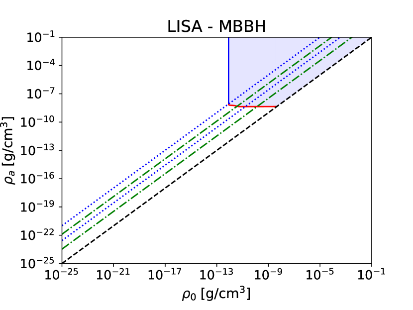
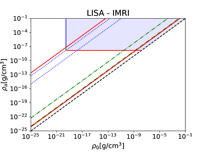
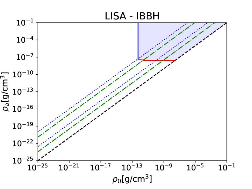
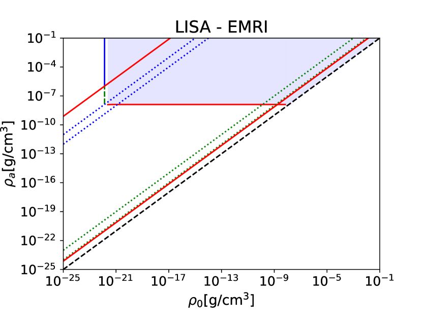
Figure 1: Maps of the detection prospects with LISA for different events, in terms of the dark matter parameters $\rho_{0}$ and $\rho_{a}$. The lower right area below the black dashed line is not physical. The shaded upper right area shows the region of the parameter space where the dark matter environment can be detected.

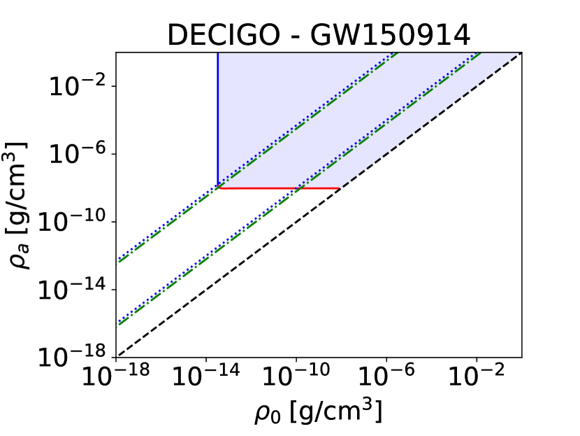
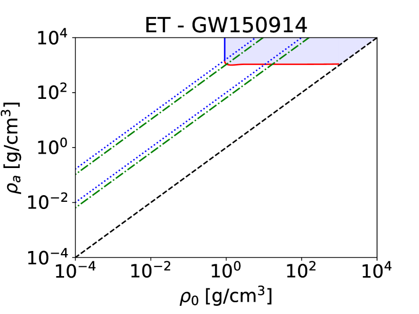
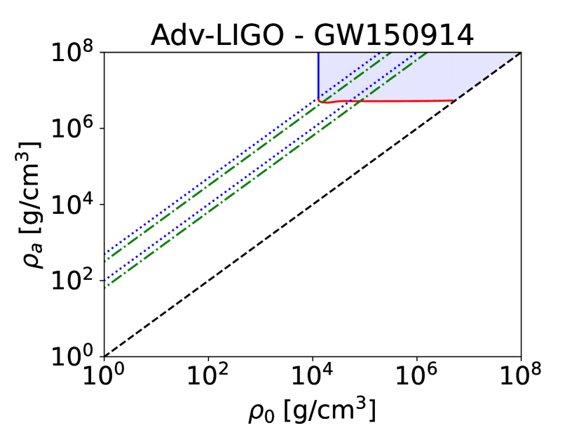
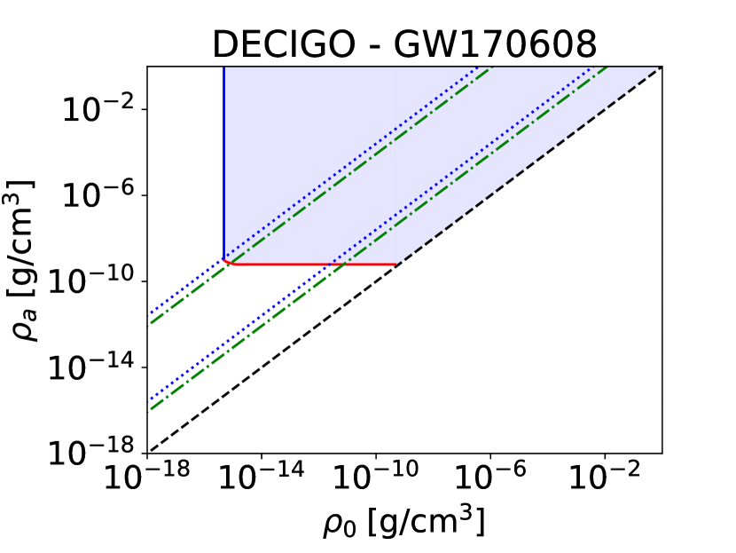
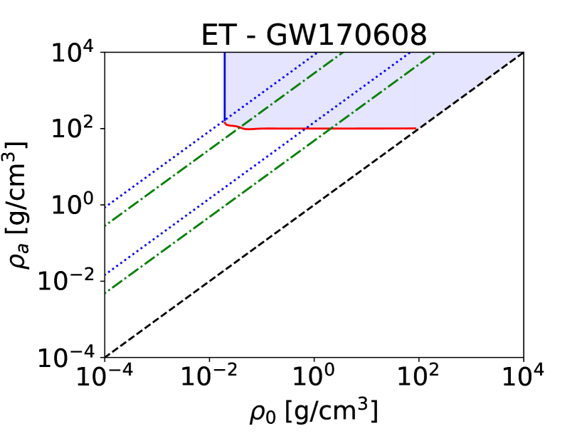
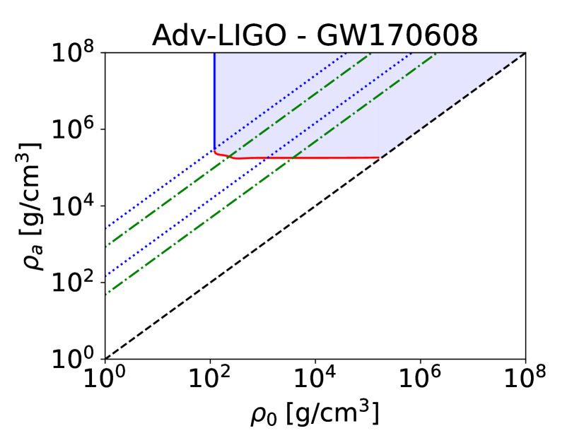
Figure 2: Maps of the detection prospects for three different interferometers (from left-to-right: DECIGO, ET, and Adv-LIGO), for the two events GW150914 (upper row) and GW170608 (lower row).

We show in Figs. 1 and 2 our results for the detection thresholds in the $(\rho_{0},\rho_{a})$, following the Fisher matrix analysis described in Sec. V. Let us first describe the LISA-MBBH case, shown in the upper left panel in Fig. 1. The lower diagonal black dashed line is the lower limit $y=1$ ($c_{s}=c$) on the physical part of the parameter space. The parallel blue dotted lines are the thresholds $y_{{\rm acc},1}^{+}$ and $y_{{\rm acc},1}^{-}$ while the green dot-dashed lines are the thresholds $y_{{\rm acc},2}^{+}$ and $y_{{\rm acc},2}^{-}$ (constant-$y$ lines are parallel to the diagonal $y=1$ in the $(\log(\rho_{0}),\log(\rho_{a}))$ logarithmic plane). Because $\nu>0.16$ there is no dynamical friction.

Then, above the upper blue dotted line $y_{{\rm acc},1}^{+}$, we are in the large-$y$ regime (94) and there is no constraint on $\rho_{a}$. Thus, we obtain a vertical line $\rho_{0}>\rho_{0\star}$ with $\rho_{0\star}\simeq 8\times 10^{-13}{\rm g/cm}^{3}$ This should be compared with the simple estimate (96), which gives $\rho_{0\star}\gtrsim 10^{-14}{\rm g/cm}^{3}$ as we have $f_{\rm min}\simeq 6\times 10^{-5}\,{\rm Hz}$. As expected the more accurate Fisher analysis gives a higher value but we roughly recover the same order of magnitude. This gives the shaded area to the right of $\rho_{0\star}$ and above the line $y_{{\rm acc},1}^{+}$ as a region where DM would be detected, mostly because of the accretion contribution $\Psi_{{\rm acc},1}$ on the larger BH.

Between the lines $y_{{\rm acc},1}^{+}$ and $y=1$, we are in the low-$y$ regime (98) where the phase depends on both $\rho_{0}$ and $\rho_{a}$. The Fisher matrix analysis gives an almost flat boundary curve $\rho_{a}>\rho_{a\star}$ with $\rho_{a\star}\simeq 5\times 10^{-9}{\rm g/cm}^{3}$ This should be compared with the simple estimate (101), which gives $\rho_{a\star}\gtrsim 10^{-11}{\rm g/cm}^{3}$. Again, the more accurate Fisher analysis gives a higher value but we roughly recover the same order of magnitude. In particular, the estimates (96) and (101) correctly predict the large hierarchy between the thresholds $\rho_{0\star}$ and $\rho_{a\star}$. This gives the remaining shaded area between the lines $y_{{\rm acc},1}^{+}$ and $y=1$, above $\rho_{a\star}$, as a region where DM would be detected, mostly because of the accretion contribution $\Psi_{{\rm acc},1}$ on the larger BH, but now in the low-velocity self-regulated regime.

The same behaviors are found for the LISA-IBBH case, shown in the lower left panel in Fig. 1. In particular, with $f_{\rm min}\simeq 6\times 10^{-4}\,{\rm Hz}$, Eqs.(96) and (101) give the simple estimates $\rho_{0\star}\gtrsim 10^{-14}{\rm g/cm}^{3}$ and $\rho_{a\star}\gtrsim 10^{-9}{\rm g/cm}^{3}$, whereas the detailed Fisher matrix inversion gives the more accurate results $\rho_{0\star}\simeq 5\times 10^{-13}{\rm g/cm}^{3}$ and $\rho_{a\star}\simeq 3\times 10^{-8}{\rm g/cm}^{3}$.

Let us now consider the LISA-IMRI case, shown in the upper right panel in Fig. 1. In addition to the thresholds $\{y_{{\rm acc},1}^{+},y_{{\rm acc},1}^{-}\}$ and $\{y_{{\rm acc},2}^{+},y_{{\rm acc},2}^{-}\}$, the red solid lines show the dynamical friction thresholds $\{y_{{\rm df},2}^{+},y_{{\rm df},2}^{-}\}$. Above the upper line $y_{{\rm df},2}^{+}$ we are again in the large-$y$ regime (94), with a vertical bound $\rho_{0\star}=3\times 10^{-20}{\rm g/cm}^{3}$. This is again within a factor 100 of the simple estimate (96), which gives $\rho_{0\star}\gtrsim 10^{-21}{\rm g/cm}^{3}$ with $f_{\rm min}\simeq 6\times 10^{-3}\,{\rm Hz}$. In the narrow band $y_{{\rm acc},1}^{+}<y<y_{{\rm df},2}^{+}$ we are in the intermediate regime (97), with a weak dependence on $\rho_{a}$ through $c_{s}$ in the terms inside the brackets in Eq.(75). Thus, we still have a roughly vertical line. Below $y_{{\rm acc},1}^{+}$ we are in the low-$y$ regime (98), which is now dominated by the new dependence of the accretion term on $\rho_{a}$, which gives a roughly horizontal line with $\rho_{a\star}\simeq 2\times 10^{-8}{\rm g/cm}^{3}$. The simple estimate (101) gives $\rho_{a\star}\gtrsim 10^{-9}{\rm g/cm}^{3}$, which is again within a factor 100 of the more accurate Fisher matrix result and reproduces the large hierarchy between $\rho_{0\star}$ and $\rho_{a\star}$.

We obtain similar behaviors for the LISA-EMRI case, shown in the lower right panel in Fig. 1. With $f_{\rm min}\sim 3\times 10^{-3}\,{\rm Hz}$, the simple estimates (96) and (101) give $\rho_{0\star}\gtrsim 10^{-24}{\rm g/cm}^{3}$ and $\rho_{a\star}\gtrsim 10^{-10}{\rm g/cm}^{3}$, whereas the more accurate Fisher matrix results are $\rho_{0\star}\simeq 10^{-22}{\rm g/cm}^{3}$ and $\rho_{a\star}\simeq 10^{-8}{\rm g/cm}^{3}$.

We obtain similar behaviors in 2 for the DECIGO, ET and Adv-LIGO detectors, for stellar-mass binaries. As in the MBBH and IBBH cases, there is no dynamical friction regime. DECIGO provides constraints on DM environments that are similar to those obtained from LISA, but the ET and Adv-LIGO cannot detect the dark matter cloud for realistic densities.

Thus, in all cases the detection domain is an upper right region, delimited from the left by $\rho_{0\star}$, from below by $\rho_{a\star}$, and from the right by the diagonal $\rho_{a}=\rho_{0}$. The simple estimates (96) and (101) are typically below the exact thresholds $\rho_{0\star}$ and $\rho_{a\star}$ by a factor of up to 100, but they reproduce the main trends and the hierarchy between $\rho_{0\star}$ and $\rho_{a\star}$. The DM detection is dominated by the accretion contribution $\Psi_{\rm acc}$ on the larger BH. Above the diagonal $y_{{\rm acc},1}^{+}$, which runs through the lower-left corner of this domain, the accretion rate is proportional to $\rho_{0}$ whereas below the diagonal $y_{{\rm acc},1}^{+}$ it is proportional to $\rho_{a}$. Therefore, in the shaded domain above $y_{{\rm acc},1}^{+}$ we measure $\rho_{0}$ whereas below $y_{{\rm acc},1}^{+}$ we measure $\rho_{a}$.

	LISA	DECIGO	ET	Adv-LIGO
MBBH	$\rho_{0}>8\times 10^{-13}$ g/cm3	$\bigtimes$	$\bigtimes$	$\bigtimes$
	$\rho_{a}>5\times 10^{-9}$ g/cm3	$\bigtimes$	$\bigtimes$	$\bigtimes$
IBBH	$\rho_{0}>5\times 10^{-13}$ g/cm3	$\bigtimes$	$\bigtimes$	$\bigtimes$
	$\rho_{a}>3\times 10^{-8}$ g/cm3	$\bigtimes$	$\bigtimes$	$\bigtimes$
IMRI	$\rho_{0}>3\times 10^{-20}$ g/cm3	$\bigtimes$	$\bigtimes$	$\bigtimes$
	$\rho_{a}>2\times 10^{-8}$ g/cm3	$\bigtimes$	$\bigtimes$	$\bigtimes$
EMRI	$\rho_{0}>10^{-22}$ g/cm3	$\bigtimes$	$\bigtimes$	$\bigtimes$
	$\rho_{a}>10^{-8}$ g/cm3	$\bigtimes$	$\bigtimes$	$\bigtimes$
GW150914	$\bigtimes$	$\rho_{0}>3\times 10^{-14}$ g/cm3	$\rho_{0}>0.9$ g/cm3	$\rho_{0}>10^{4}$ g/cm3
	$\bigtimes$	$\rho_{a}>10^{-8}$ g/cm3	$\rho_{a}>10^{3}$ g/cm3	$\rho_{a}>5\times 10^{6}$ g/cm3
GW170608	$\bigtimes$	$\rho_{0}>5\times 10^{-16}$ g/cm3	$\rho_{0}>0.02$ g/cm3	$\rho_{0}>120$ g/cm3
	$\bigtimes$	$\rho_{a}>10^{-9}$ g/cm3	$\rho_{a}>101$ g/cm3	$\rho_{a}>2\times 10^{5}$ g/cm3

Table 4: Lower bounds $\rho_{0\star}$ and $\rho_{a\star}$ on the DM density parameters for a detection of the DM cloud, for various detectors and binary systems.

We summarize in Table 4 the density thresholds $\rho_{0\star}$ and $\rho_{a\star}$ above which the DM cloud can be detected, for the detectors and binary systems displayed in Figs. 1 and 2. This is only possible at much higher densities than the typical dark matter density on galaxy scales, which is about $10^{-26}$ to $10^{-23}$ g/cm³ Navarro et al. (1996, 1997); Martinsson et al. (2013); Salucci (2019). For comparison, we also note that accretion disks have a baryonic matter density below $\sim 0.1\,{\rm g/cm^{3}}$ for thin disks, and below $10^{-9}{\rm g/cm^{3}}$ for thick disks Barausse et al. (2014), with a lower bound around $10^{-16}{\rm g/cm^{3}}$. Therefore, only LISA and DECIGO could detect DM clouds with realistic bulk densities, $\rho_{0}>10^{-22}$g/cm³ for LISA-EMRI and $\rho_{0}>10^{-15}$g/cm³ for DECIGO. The detection of the scalar cloud also requires a very high value of the density parameter $\rho_{a}$, $\rho_{a}\gtrsim 10^{-8}$g/cm³. However, this is not the typical density of the DM cloud but only the density close to the Schwarzschild radius, in the accretion regime regulated by the self-interactions. On the other hand, DM clouds with densities much higher than typical baryonic accretion disks may be produced in the early universe, as discussed for instance in Berezinsky et al. (2014); Brax et al. (2020b) for several scenarios. Then, in contrast with the standard CDM case, the dark matter density field would be extremely clumpy, in the form of a distribution of small and dense clouds (in a manner somewhat similar to primordial BHs or macroscopic dark matter scenarios, but with larger-size objects).

 Detection threshold for $\rho_{\rm a}$ and parameter space

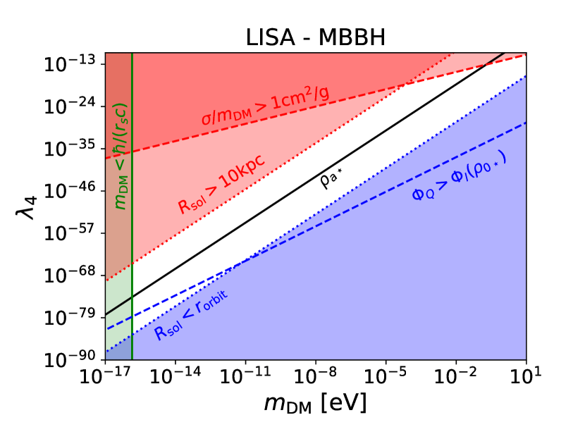
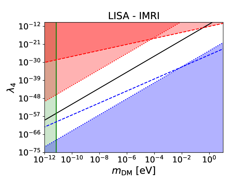
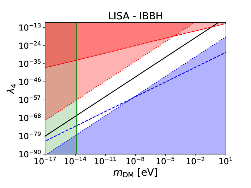
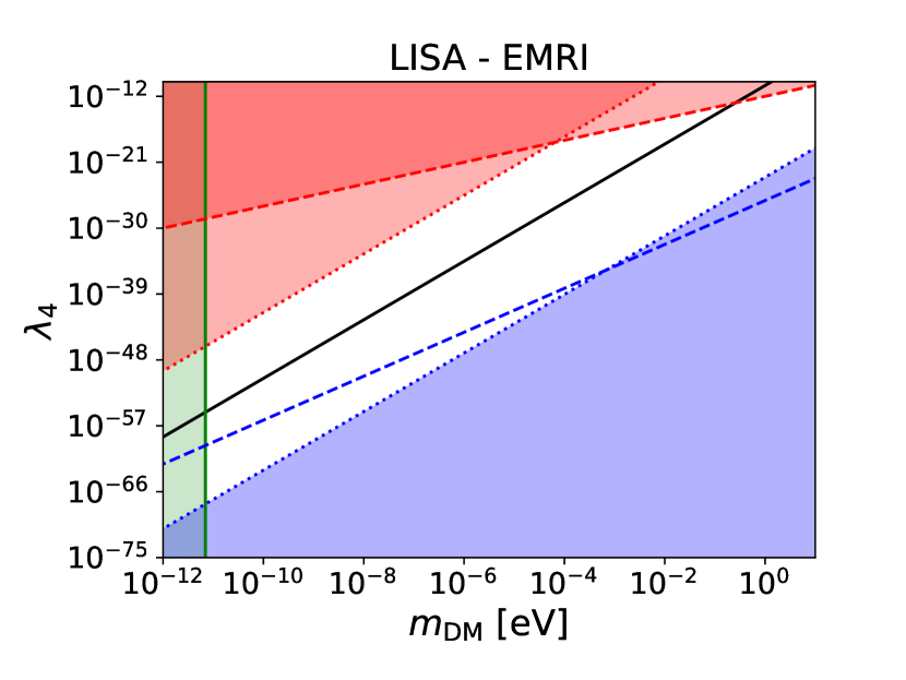
Figure 3: Domain over the parameter space ($m_{\rm DM}$, $\lambda_{4}$) where our derivations are applicable, in the case of the LISA interferometer. The white area represents the allowed parameter space. The upper left red region is excluded by observational constraints. In the lower right blue region the scalar dark matter model is allowed but the assumptions used in our computations must be revised. The black line corresponds to the detection limit obtained in Fig. 1. Parameter values above this line are beyond the detectability range of the interferometer.

In this section, we compare the detection threshold $\rho_{a\star}$ obtained in Table 4 with the allowed parameter space of our dark matter model, in the $(m_{\rm DM},\lambda_{4})$ plane. This allows us to check wether this scenario can be efficiently probed by the measurement of the gravitational waves emitted by BH binary systems embedded in such dark matter clouds. Our results are displayed in Figs. 3 and 4, representing the outcomes for LISA and DECIGO. We do not consider ET and Adv-LIGO, because they require bulk densities that are probably too high to be realistic. Various colored regions on the figures correspond to distinct limits based on either observational constraints or the regime considered in our calculations.

From Eq.(3), a detection floor $\rho_{a\star}$ corresponds to an upper ceiling for $\lambda_{4}$ that scales as $m^{4}_{\rm DM}$,

$$\rho_{a}>\rho_{a\star}:\;\;\;\lambda_{4}<\frac{4m_{\rm DM}^{4}c^{3}}{3\rho_{a\star}\hbar^{3}},$$ (102)

which reads

$$\lambda_{4}<3\times 10^{-19}\left(\frac{\rho_{a\star}}{1\,{\rm g/cm^{3}}}\right)^{-1}\left(\frac{m_{\rm DM}}{1\,{\rm eV}}\right)^{4}.$$ (103)

This ceiling is shown by the black solid line labeled $\rho_{a\star}$ that runs through the white area in Figs. 3 and 4.

We now describes the constraints that determine the parameter space of the model, with the exclusion domains shown by the colored regions in the plots. First, we require the condition (6), which also reads

$$m_{\rm DM}>\frac{\hbar c}{2{\cal G}m_{<}},\;\;\;m_{\rm DM}>7\times 10^{-11}\left(\frac{m_{<}}{1\,M_{\odot}}\right)^{-1}\;{\rm eV}.$$ (104)

This ensures the validity of the accretion rate (7) and of the dynamical friction (10), derived in Brax et al. (2020a); Boudon et al. (2022, 2023) in the large-mass limit $\partial_{r}\ll cm_{\rm DM}/\hbar$. This condition excludes the green area marked by a vertical line on the left in the figures, labeled $m_{\rm DM}<\hbar/(r_{s}c)$.

Observations of cluster mergers, such as the bullet cluster, provide an upper bound on the dark matter cross-section, $\sigma/m_{\rm DM}\lesssim 1$ cm²/g Randall et al. (2008). This gives the upper bound Brax et al. (2019)

$$\lambda_{4}<10^{-12}\left(\frac{m}{1\,{\rm eV}}\right)^{\frac{3}{2}},$$ (105)

shown by the dashed red line in the upper left corner of the figures, labeled $\sigma/m_{\rm DM}>1\,{\rm cm}^{2}/{\rm g}$.

Another observational limit, shown by the upper left red dotted line labeled $R_{\rm sol}>10\,{\rm kpc}$, is the maximum size of the dark matter solitons. As we wish such solitons to fit inside galaxies, we require $R_{\rm sol}<10$ kpc. This gives the upper bound

$$\lambda_{4}<0.03\left(\frac{R_{\rm sol}}{10\,{\rm kpc}}\right)^{2}\left(\frac{m_{\rm DM}}{1\,{\rm eV}}\right)^{4}.$$ (106)

This condition is actually parallel to the detection threshold (103) and somewhat above it in the Figs. 1 and 2. Therefore, the largest solitons would not be detected by GW. This will be more clearly seen in Sec. VI.5 below.

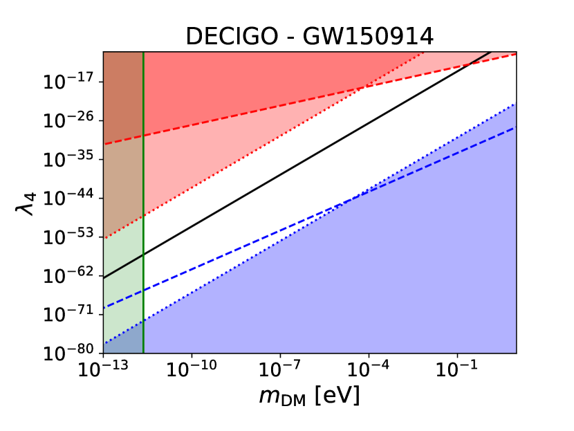
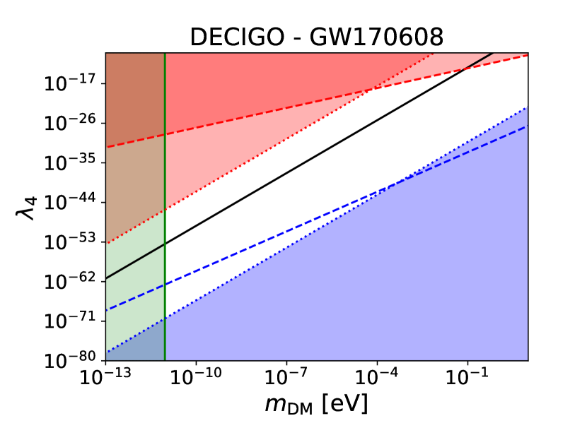
Figure 4: Domain over the parameter space ($m_{\rm DM}$, $\lambda_{4}$) where our derivations are applicable and detection threshold, as in Fig. 3 but for the interferometer DECIGO.

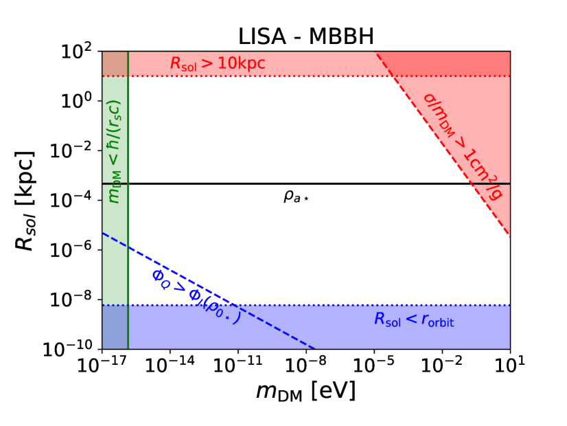
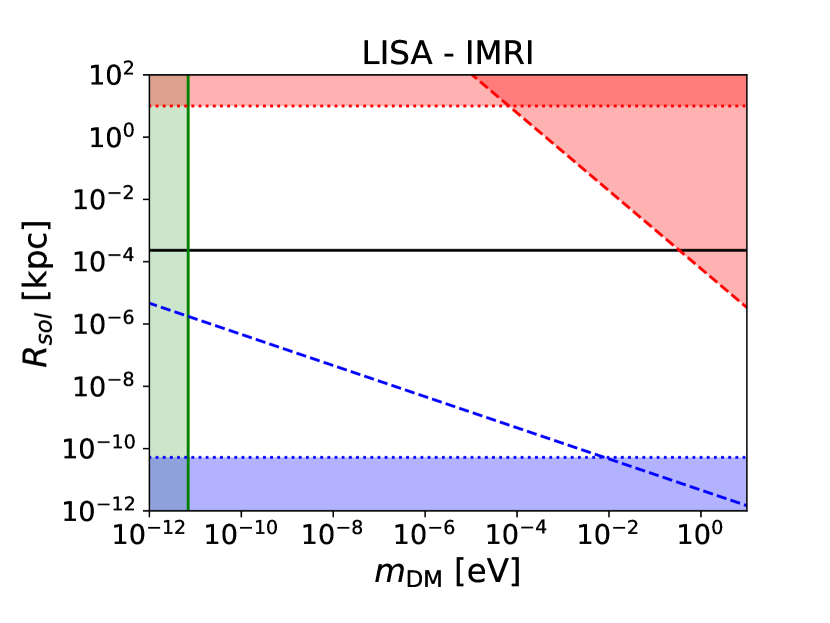
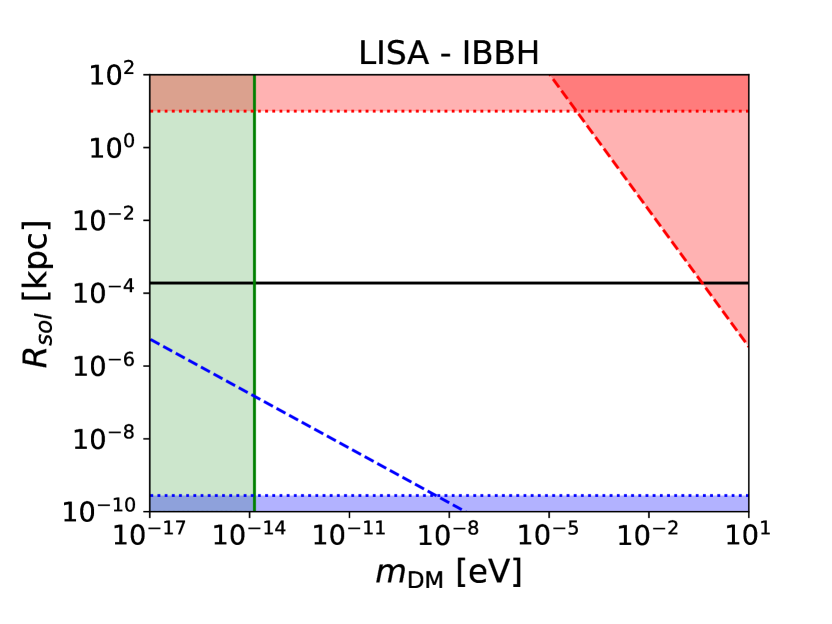
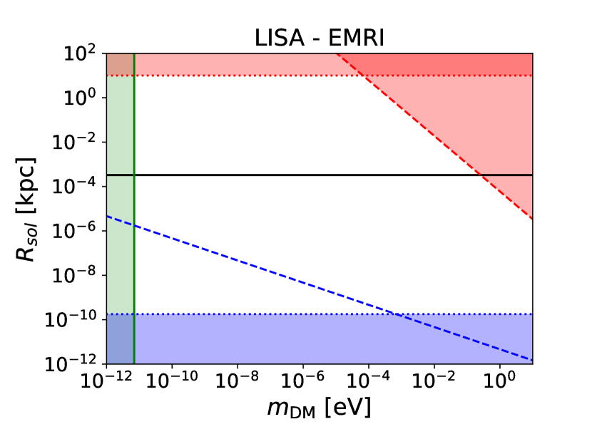
Figure 5: Domain over the parameter space ($m_{\rm DM}$, $R_{\rm sol})$ where our derivations are applicable and detection threshold, in the case of the LISA interferometer as in Fig. 3

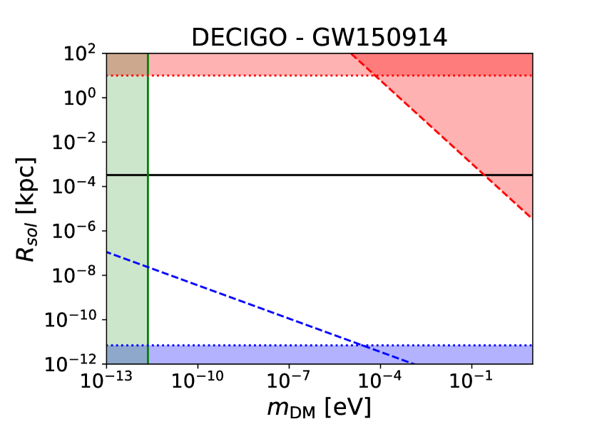
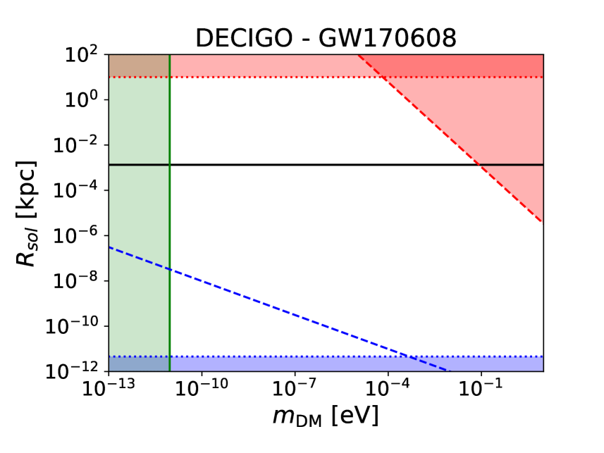
Figure 6: Domain over the parameter space ($m_{\rm DM}$, $R_{\rm sol})$ where our derivations are applicable and detection threshold, in the case of the DECIGO interferometer as in Fig. 4.

Our derivation of the accretion rate (7) and of the dynamical friction (10) assumes that the self-interaction dominates over the quantum pressure Brax et al. (2020a); Boudon et al. (2022, 2023), in contrast with FDM scenarios where the latter dominates and the self-interactions are neglected. The self-interaction potential reads $\Phi_{I}=c^{2}\rho/\rho_{a}$, whereas the quantum pressure reads $\Phi_{Q}=-\hbar^{2}\nabla^{2}\sqrt{\rho}/(2m_{\rm DM}^{2}\sqrt{\rho})$. This gives the condition $c^{2}\rho/\rho_{a}>\hbar^{2}/(r^{2}m_{\rm DM}^{2})$, where $\rho$ and $r$ are the density and length scale of interest. This condition near the BH horizon, with $\rho\sim\rho_{a}$ and $r\sim r_{s}$, coincides with the condition (104) and is thus already enforced. Requiring that this also holds over the bulk of the soliton, at density $\rho_{0}$ and radius $r\sim R_{\rm sol}$, gives the additional constraint

$$\lambda_{4}>\frac{8m_{\rm DM}^{3}\sqrt{\cal G}}{3\sqrt{\pi}\hbar^{2}\sqrt{\rho_{0}}},$$ (107)

which reads

$$\lambda_{4}>6\times 10^{-38}\left(\frac{\rho_{0}}{1\,{\rm g/cm^{3}}}\right)^{-\frac{1}{2}}\left(\frac{m_{\rm DM}}{1\,{\rm eV}}\right)^{3}.$$ (108)

For the density $\rho_{0\star}$ this is shown by the blue dashed line labeled $\Phi_{Q}>\Phi_{I}(\rho_{0\star})$. Below this threshold the model itself is not excluded, but our computations should be be revised as the bulk of the soliton is now governed by the quantum pressure instead of the self-interactions. However, if the bulk density is greater than $\rho_{0\star}$ this region moves down to smaller values of $\lambda_{4}$. Therefore, the blue dashed line is not a strict limit.

Lastly, the area below the blue dotted line labeled $R_{\rm sol}<r_{\rm orbit}$ represents the parameter space where the soliton size is smaller than the initial orbital radius of the binary system during the measurement. To ensure the applicability of our calculation across all frequencies, we must thus consider

$$\lambda_{4}>\frac{16{\cal G}cm_{\rm DM}^{4}r_{\rm orbit}^{2}}{3\pi\hbar^{3}},$$ (109)

which reads

$$\lambda_{4}>3\times 10^{-10}\left(\frac{m_{\rm DM}}{1\,{\rm eV}}\right)^{4}\left(\frac{r_{\rm orbit}}{1\,{\rm pc}}\right)^{2}.$$ (110)

For $r_{\rm orbit}$ we take the maximum orbital radius, computed with Kepler’s third law at the earliest measurement time, associated with the frequency $f_{\rm obs}(4\,{\rm yr})$. This constraint is parallel to the soliton-size condition (106) and to the detection threshold $\rho_{a\star}$ in Eq.(103).

Hence, the white area in the parameter space indicates where the dark matter model is realistic and all our calculations apply successfully. More precisely, the upper bounds, associated with the red exclusion regions, correspond to unphysical regions of the parameter space, whereas the lower bounds, associated with blue exclusion regions, only correspond to regions where some of our computations should be revised. However, where they fall within the detection domain, below the black solid line, it should remain possible to detect the dark matter environment.

We can see in Fig. 3 and Fig.4 that in all cases the detection threshold $\rho_{a\star}$ runs through the white area. In particular, it is parallel but below the upper bound associated with the soliton size limit and above the lower bound associated with the orbital radius limit. Thus, whereas the largest solitons cannot be detected, a large part of the available parameter space could lead to detection by interferometers such as LISA and DECIGO. Whereas LISA probes models with a scalar mass $10^{-15}\lesssim m_{\rm DM}\lesssim 1$ eV, DECIGO is restricted to $10^{-12}\lesssim m_{\rm DM}\lesssim 1$ eV.

 Constraints on the soliton radius

The two parameters $m_{\rm DM}$ and $\lambda_{4}$ also determine the soliton size $R_{\rm sol}$, as seen in Eqs.(3) and (4). As $R_{\rm sol}$ is more relevant for observational purposes than the coupling $\lambda_{4}$, we show in Figs. 5 and 6 the application domain of our computations and the detection threshold $\rho_{a\star}$ in the parameter space $(m_{\rm DM},R_{\rm sol})$, instead of the plane $(m_{\rm DM},\lambda_{4})$ shown in Figs. 3 and 4 above.

We can see that no experiment can probe galactic-size soltons, $R_{\rm sol}\gtrsim 1$ kpc, that could be invoked to alleviate the small-scale problems encountered by the standard CDM scenario. At best, LISA and DECIGO can probe models associated with $10^{-7}{\rm pc}\lesssim R_{\rm sol}\lesssim 0.1\,{\rm pc}$. These astrophysical scales range from a percent of astronomical unit to a tenth of the typical distance between stars in the Milky Way. Nevertheless, this is still a large fraction of the parameter space.

Scalar dark matter scenarios associated with solitons of such subgalactic size cannot be constrained by cosmological probes, such as the Lyman-$\alpha$ forest, or galaxy rotation curves. Their moderate density also evades microlensing detections. Therefore, their impact on the gravitational waveforms emitted by binary systems that they could contain would be a key probe of these dark matter scenarios.

 Comparison with other results

Our results for the minimal value $\rho_{0\star}$ of the bulk density $\rho_{0}$ that can be measured (i.e., its detection threshold) are close to the results obtained in Fig. 2 of Cardoso  and Maselli (2020) from collisionless dynamical friction, for the DECIGO, ET and ADv-LIGO events and for the LISA interferometer in the MBBH and IBBH cases, and somewhat more optimistic than the Bayesian analysis of Santoro et al. (2023). While, as noticed above, the scalings of the expression (10) for the dynamical friction drag force are quite general and apply to most media, from collisionless particles to gaseous media and scalar-field dark matter scenarios, up to some numerical factors, it is not the reason for the similarity in our outcomes. Our main determinant for the detection threshold, as outlined in Eq.(96), is the accretion drag force, not the dynamical friction. However, in the high-frequency regime the accretion contribution (74) shows the same scaling as the dynamical friction contribution (75), $\Psi\sim({\cal G}^{3}{\cal M}^{2}\rho_{0}/c^{6})(\pi{\cal G}{\cal M}f/c^{3})^{-16/3}$, up to numerical factors and ratios of the binary masses. This explains why we recover similar results to those of Fig. 2 of Cardoso  and Maselli (2020) for the cases where the binary masses are similar and those mass ratios are of the order of unity.

However, for the IMRI and EMRI cases with the LISA interferometer, our findings are more promising as we obtain detection thresholds that are lower by factors $\sim 10^{3}$ as compared with Fig. 2 of Cardoso  and Maselli (2020). This is because the accretion contribution (74) is greater than the dynamical friction contribution (75) that would be associated with the most massive BH by a factor $m_{i}^{2}/(m\mu)\sim m_{>}/m_{<}\sim 1/\nu$, which reaches $10^{3}$ and $10^{4}$ for IMRI and EMRI.

Here we note that our results (74) and (75) actually differ from the Bondi-accretion and collisionless dynamical friction results of Cardoso  and Maselli (2020) by powers or $\nu$, which are relevant in case of IMRI and EMRI. As compared with Cardoso  and Maselli (2020), our contribution from the accretion drags is enhanced by the factor $2m_{i}^{2}/(m\mu)\sim 2m_{>}/m_{<}\sim 2/\nu$ associated with the accretion onto the more massive BH. This term originates from the factor $\overset{\bm{.}}{m}\vphantom{m}/m$ in Eq.(36), which comes from the drift of the Runge-Lenz vector (35). It seems that the expressions used in Cardoso  and Maselli (2020) only take into account the term $2\overset{\bm{.}}{\mu}\vphantom{\mu}/\mu$ in the accretion drag, that is, the accretion contribution to the force $F(t)$ in Eqs.(29) and (36), and neglect the factor $\overset{\bm{.}}{m}\vphantom{m}/m$.

Our contribution (75) for dynamical friction shows the same scalings as in Cardoso  and Maselli (2020). However, as we only include the contribution from the smaller BH, because of the frequency thresholds, its value is reduced because of the terms $m_{i}^{3}/(\mu^{2}m)$, which yield a suppression factor $\sim\nu^{3}$ for small $\nu$. This is because we consider a self-interacting scalar-field environment instead of collisionless particles. This shows the possible impact of the properties of the medium on the gravitational drag. However, in our case this term is subdominant as compared with the accretion contribution and it may be difficult to estimate its precise value from observations.

Our detection thresholds are much lower than those shown in Fig. 1 of Cardoso  and Maselli (2020) for collisionless accretion. This is because the accretion of scalar field dark matter if much more efficient than that of collisionless particles (but less efficient than that of a perfect gas at low Mach numbers), see Boudon et al. (2022, 2023). Indeed, pressure forces restrict tangential motion and funnel particles in the radial direction (Shapiro  and Teukolsky, 1983). This also gives a different velocity and frequency dependence for the accretion drag associated with collisionless and self-interacting dark matter.

II. onclusion

The detection of GWs has already given important results for fundamental physics, e.g. the near equality between the speed of GWs and the speed of light Abbott et al. (2017, 2019b); Liu et al. (2020). In this paper, we suggest that future experiments could reveal some key properties of dark matter. As an example, we focus on scalar dark matter with quartic self-interactions and assume that the dark matter density of the Universe is due to the misalignment mechanism for the scalar field. Locally inside galaxies, these models can give rise to dark matter solitons of finite size where gravity and the repulsive self-interaction pressure balance exactly. This regime applies when the size of the solitons is much larger than the de Broglie wavelength of the scalar particles. In this case, these solitons could be pervasive in each galaxy and BHs could naturally be embedded within these scalar clouds when inspiralling towards each other in binary systems. The scalar clouds have three effects on the orbits of the binary systems. First, the gravity of the cloud modifies the trajectories of the BHs. Second, dark matter accretes onto the BHs and slows them down. Third, in the supersonic regime the dynamical friction due to the gravitational interaction between the BHs and distant streamlines further slows them down. These effects can lead to significant deviations of the binary orbits and therefore to perturbations of the GW signal emitted by the pair of BHs. The cloud gravity gives a -3PN contribution to the gravitational waveform. The accretion gives a -4PN or -5.5PN effect at low or high frequency, whereas the dynamical friction gives a -5.5PN contribution. As such, these effects are not degenerate with the relativistic corrections that appear at higher post-Newtonian orders.

For a large part of the scalar dark matter parameter space, future experiments such as LISA and DECIGO should be able to observe the impact on GW of these dark matter environments, provided binary systems are embedded within such scalar clouds. This would give new clues about the nature of dark matter. Within the framework of the scalar field models with quartic self-interactions studied in this paper, this would give indications on the value of the bulk dark matter density $\rho_{0}$ as well as the characteristic density $\rho_{a}$ of Eq.(3), that is, the combination $m_{\rm DM}^{4}/\lambda_{4}$. This would also give an indirect estimate of the size $R_{\rm sol}$ of the solitons, from Eq.(4). The relatively high values of $\rho_{0}$ required for detection, at least a few hundred times above the dark matter density in the Solar system for EMRI with LISA, suggest that this probe is mostly relevant for scenarios where the scalar clouds form at high redshifts, giving rise to a very clumpy dark matter distribution. The fact that we have not detected such dark matter effects in the ET and LIGO events is consistent with the high bulk densities, $\rho_{0}\gtrsim 1\,{\rm g/cm}^{3}$, that are needed to allow a detection with these interferometers.

On the other hand, the scenarios that can be probed through their impact on binary GW waveforms, studied in this paper, correspond to small clouds below $0.1$ pc that cannot be constrained by cosmological probes or galaxy rotation curves, while there density is still too small to be detected by microlensing. Therefore, GW waveforms would be a key probe of these dark matter models.

Perturbations to the gravitational waveforms may result from diverse environments, including gaseous clouds or dark matter halos associated with other dark matter models. In all cases where such environments are present, we can expect accretion and dynamical friction to occur and slow down the orbital motion. It would be interesting to study whether one can discriminate between these different environments. As shown in this paper, to do so we could use the magnitude of these two effects and also the parts in the data sequence where dynamical friction appears to be active or not. Indeed, depending on the medium dynamical friction is expected to be negligible in some regimes, such as subsonic velocities. If one can extract such conditions from the data, one may gain some useful information on the environment of the binary systems. We leave such studies to future works.

knowledgments

A.B. would like to thank Andrea Maselli for his help in the first stage of this project.

References

- Chandrasekhar (1943) S. Chandrasekhar, Dynamical Friction. I. General Considerations: the Coefficient of Dynamical Friction, Astrophys. J. 97, 255 (1943).
- Dokuchaev (1964) V. P. Dokuchaev, Emission of Magnetoacoustic Waves in the Motion of Stars in Cosmic Space., SvA 8, 23 (1964).
- Ruderman and Spiegel (1971) M. A. Ruderman and E. A. Spiegel, Galactic Wakes, Astrophys. J. 165, 1 (1971).
- Rephaeli and Salpeter (1980) Y. Rephaeli and E. E. Salpeter, Flow past a massive object and the gravitational drag, ApJ 240, 20 (1980).
- Ostriker (1999) E. C. Ostriker, Dynamical friction in a gaseous medium, Astrophys. J. 513, 252 (1999), arXiv:astro-ph/9810324.
- Hui et al. (2017) L. Hui, J. P. Ostriker, S. Tremaine, and E. Witten, Ultralight scalars as cosmological dark matter, Phys. Rev. D 95, 043541 (2017), arXiv:1610.08297.
- Lancaster et al. (2020) L. Lancaster, C. Giovanetti, P. Mocz, Y. Kahn, M. Lisanti, and D. N. Spergel, Dynamical Friction in a Fuzzy Dark Matter Universe, JCAP 01 (2020) 001, arXiv:1909.06381.
- Annulli et al. (2020a) L. Annulli, V. Cardoso, and R. Vicente, Response of ultralight dark matter to supermassive black holes and binaries, Phys. Rev. D 102, 063022 (2020a), arXiv:2009.00012.
- Traykova et al. (2021) D. Traykova, K. Clough, T. Helfer, E. Berti, P. G. Ferreira, and L. Hui, Dynamical friction from scalar dark matter in the relativistic regime, Phys. Rev. D 104, 103014 (2021), arXiv:2106.08280.
- Chowdhury et al. (2021) D. D. Chowdhury, F. C. van den Bosch, V. H. Robles, P. van Dokkum, H.-Y. Schive, T. Chiueh, and T. Broadhurst, On the Random Motion of Nuclear Objects in a Fuzzy Dark Matter Halo, Astrophys. J. 916, 27 (2021), arXiv:2105.05268.
- Wang and Easther (2022) Y. Wang and R. Easther, Dynamical friction from ultralight dark matter, Phys. Rev. D 105, 063523 (2022), arXiv:2110.03428.
- Vicente and Cardoso (2022) R. Vicente and V. Cardoso, Dynamical friction of black holes in ultralight dark matter, Phys. Rev. D 105, 083008 (2022), arXiv:2201.08854.
- Traykova et al. (2023) D. Traykova, R. Vicente, K. Clough, T. Helfer, E. Berti, P. G. Ferreira, and L. Hui, Relativistic drag forces on black holes from scalar dark matter clouds of all sizes, (2023), arXiv:2305.10492.
- Brax et al. (2020a) P. Brax, J. A. R. Cembranos, and P. Valageas, Fate of scalar dark matter solitons around supermassive galactic black holes, Phys. Rev. D 101, 023521 (2020a), arXiv:1909.02614.
- Boudon et al. (2022) A. Boudon, P. Brax, and P. Valageas, Subsonic accretion and dynamical friction for a black hole moving through a self-interacting scalar dark matter cloud, Phys. Rev. D 106, 043507 (2022), arXiv:2204.09401.
- Boudon et al. (2023) A. Boudon, P. Brax, and P. Valageas, Supersonic friction of a black hole traversing a self-interacting scalar dark matter cloud, (2023), arXiv:2307.15391.
- Roszkowski et al. (2018) L. Roszkowski, E. M. Sessolo, and S. Trojanowski, WIMP dark matter candidates and searches—current status and future prospects, Rept. Prog. Phys. 81, 066201 (2018), arXiv:1707.06277.
- Arcadi et al. (2018) G. Arcadi, M. Dutra, P. Ghosh, M. Lindner, Y. Mambrini, M. Pierre, S. Profumo, and F. S. Queiroz, The waning of the WIMP? A review of models, searches, and constraints, Eur. Phys. J. C 78, 203 (2018), arXiv:1703.07364.
- Goodman (2000) J. Goodman, Repulsive dark matter, New Astron. 5, 103 (2000), arXiv:astro-ph/0003018.
- Schive et al. (2014a) H.-Y. Schive, T. Chiueh, and T. Broadhurst, Cosmic Structure as the Quantum Interference of a Coherent Dark Wave, Nature Phys. 10, 496 (2014a), arXiv:1406.6586.
- Schive et al. (2014b) H.-Y. Schive, M.-H. Liao, T.-P. Woo, S.-K. Wong, T. Chiueh, T. Broadhurst, and W. Y. P. Hwang, Understanding the Core-Halo Relation of Quantum Wave Dark Matter from 3D Simulations, Phys. Rev. Lett. 113, 261302 (2014b), arXiv:1407.7762.
- Arbey et al. (2001) A. Arbey, J. Lesgourgues, and P. Salati, Quintessential haloes around galaxies, Phys. Rev. D 64, 123528 (2001), arXiv:astro-ph/0105564.
- Chavanis (2011) P.-H. Chavanis, Mass-radius relation of Newtonian self-gravitating Bose-Einstein condensates with short-range interactions: I. Analytical results, Phys. Rev. D 84, 043531 (2011), arXiv:1103.2050.
- Chavanis and Delfini (2011) P. H. Chavanis and L. Delfini, Mass-radius relation of Newtonian self-gravitating Bose-Einstein condensates with short-range interactions: II. Numerical results, Phys. Rev. D 84, 043532 (2011), arXiv:1103.2054.
- Marsh and Pop (2015) D. J. E. Marsh and A.-R. Pop, Axion dark matter, solitons and the cusp–core problem, Mon. Not. Roy. Astron. Soc. 451, 2479 (2015), arXiv:1502.03456.
- Calabrese and Spergel (2016) E. Calabrese and D. N. Spergel, Ultra-Light Dark Matter in Ultra-Faint Dwarf Galaxies, Mon. Not. Roy. Astron. Soc. 460, 4397 (2016), arXiv:1603.07321.
- Chen et al. (2017) S.-R. Chen, H.-Y. Schive, and T. Chiueh, Jeans Analysis for Dwarf Spheroidal Galaxies in Wave Dark Matter, Mon. Not. Roy. Astron. Soc. 468, 1338 (2017), arXiv:1606.09030.
- Schwabe et al. (2016) B. Schwabe, J. C. Niemeyer, and J. F. Engels, Simulations of solitonic core mergers in ultralight axion dark matter cosmologies, Phys. Rev. D 94, 043513 (2016), arXiv:1606.05151.
- Veltmaat and Niemeyer (2016) J. Veltmaat and J. C. Niemeyer, Cosmological particle-in-cell simulations with ultralight axion dark matter, Phys. Rev. D 94, 123523 (2016), arXiv:1608.00802.
- González-Morales et al. (2017) A. X. González-Morales, D. J. E. Marsh, J. Peñarrubia, and L. A. Ureña López, Unbiased constraints on ultralight axion mass from dwarf spheroidal galaxies, Mon. Not. Roy. Astron. Soc. 472, 1346 (2017), arXiv:1609.05856.
- Robles and Matos (2012) V. H. Robles and T. Matos, Flat Central Density Profile and Constant DM Surface Density in Galaxies from Scalar Field Dark Matter, Mon. Not. Roy. Astron. Soc. 422, 282 (2012), arXiv:1201.3032.
- Bernal et al. (2018) T. Bernal, L. M. Fernández-Hernández, T. Matos, and M. A. Rodríguez-Meza, Rotation curves of high-resolution LSB and SPARC galaxies with fuzzy and multistate (ultralight boson) scalar field dark matter, Mon. Not. Roy. Astron. Soc. 475, 1447 (2018), arXiv:1701.00912.
- Mocz et al. (2017) P. Mocz, M. Vogelsberger, V. H. Robles, J. Zavala, M. Boylan-Kolchin, A. Fialkov, and L. Hernquist, Galaxy formation with BECDM – I. Turbulence and relaxation of idealized haloes, Mon. Not. Roy. Astron. Soc. 471, 4559 (2017), arXiv:1705.05845.
- Mukaida et al. (2017) K. Mukaida, M. Takimoto, and M. Yamada, On Longevity of I-ball/Oscillon, JHEP 03 (2017) 122, arXiv:1612.07750.
- Vicens et al. (2018) J. Vicens, J. Salvado, and J. Miralda-Escudé, Bosonic dark matter halos: excited states and relaxation in the potential of the ground state, (2018), arXiv:1802.10513.
- Bar et al. (2018) N. Bar, D. Blas, K. Blum, and S. Sibiryakov, Galactic rotation curves versus ultralight dark matter: Implications of the soliton-host halo relation, Phys. Rev. D 98, 083027 (2018), arXiv:1805.00122.
- Eby et al. (2019) J. Eby, K. Mukaida, M. Takimoto, L. C. R. Wijewardhana, and M. Yamada, Classical nonrelativistic effective field theory and the role of gravitational interactions, Phys. Rev. D 99, 123503 (2019), arXiv:1807.09795.
- Bar-Or et al. (2019) B. Bar-Or, J.-B. Fouvry, and S. Tremaine, Relaxation in a Fuzzy Dark Matter Halo, Astrophys. J. 871, 28 (2019), arXiv:1809.07673.
- Marsh and Niemeyer (2019) D. J. E. Marsh and J. C. Niemeyer, Strong Constraints on Fuzzy Dark Matter from Ultrafaint Dwarf Galaxy Eridanus II, Phys. Rev. Lett. 123, 051103 (2019), arXiv:1810.08543.
- Chavanis (2019) P.-H. Chavanis, Predictive model of BEC dark matter halos with a solitonic core and an isothermal atmosphere, Phys. Rev. D 100, 083022 (2019), arXiv:1810.08948.
- Emami et al. (2020) R. Emami, T. Broadhurst, G. Smoot, T. Chiueh, and H. N. Luu, Soliton solution for the central dark mass in 47-Tuc globular cluster and implications for the axiverse, Phys. Rev. D 101, 063006 (2020), arXiv:1806.04518.
- Levkov et al. (2018) D. G. Levkov, A. G. Panin, and I. I. Tkachev, Gravitational Bose-Einstein condensation in the kinetic regime, Phys. Rev. Lett. 121, 151301 (2018), arXiv:1804.05857.
- Broadhurst et al. (2020) T. Broadhurst, I. de Martino, H. N. Luu, G. F. Smoot, and S. H. H. Tye, Ghostly Galaxies as Solitons of Bose-Einstein Dark Matter, Phys. Rev. D 101, 083012 (2020), arXiv:1902.10488.
- Hayashi and Obata (2020) K. Hayashi and I. Obata, Non-sphericity of ultralight axion dark matter haloes in the Galactic dwarf spheroidal galaxies, Mon. Not. Roy. Astron. Soc. 491, 615 (2020), arXiv:1902.03054.
- Bar et al. (2019) N. Bar, K. Blum, J. Eby, and R. Sato, Ultralight dark matter in disk galaxies, Phys. Rev. D 99, 103020 (2019), arXiv:1903.03402.
- García et al. (2023) R. G. García, P. Brax, and P. Valageas, Solitons and halos for self-interacting scalar dark matter, (2023), arXiv:2304.10221.
- Preskill et al. (1983) J. Preskill, M. B. Wise, and F. Wilczek, Cosmology of the Invisible Axion, Phys. Lett. B 120, 127 (1983).
- Abbott and Sikivie (1983) L. F. Abbott and P. Sikivie, A Cosmological Bound on the Invisible Axion, Phys. Lett. B 120, 133 (1983).
- Dine and Fischler (1983) M. Dine and W. Fischler, The Not So Harmless Axion, Phys. Lett. B 120, 137 (1983).
- Arvanitaki et al. (2020) A. Arvanitaki, S. Dimopoulos, M. Galanis, L. Lehner, J. O. Thompson, and K. Van Tilburg, Large-misalignment mechanism for the formation of compact axion structures: Signatures from the QCD axion to fuzzy dark matter, Phys. Rev. D 101, 083014 (2020), arXiv:1909.11665.
- Hu et al. (2000) W. Hu, R. Barkana, and A. Gruzinov, Cold and fuzzy dark matter, Phys. Rev. Lett. 85, 1158 (2000), arXiv:astro-ph/0003365.
- Johnson and Kamionkowski (2008) M. C. Johnson and M. Kamionkowski, Dynamical and Gravitational Instability of Oscillating-Field Dark Energy and Dark Matter, Phys. Rev. D 78, 063010 (2008), arXiv:0805.1748.
- Hwang and Noh (2009) J.-c. Hwang and H. Noh, Axion as a Cold Dark Matter candidate, Phys. Lett. B 680, 1 (2009), arXiv:0902.4738.
- Park et al. (2012) C.-G. Park, J.-c. Hwang, and H. Noh, Axion as a cold dark matter candidate: low-mass case, Phys. Rev. D 86, 083535 (2012), arXiv:1207.3124.
- Hlozek et al. (2015) R. Hlozek, D. Grin, D. J. E. Marsh, and P. G. Ferreira, A search for ultralight axions using precision cosmological data, Phys. Rev. D 91, 103512 (2015), arXiv:1410.2896.
- Cembranos et al. (2016) J. A. R. Cembranos, A. L. Maroto, and S. J. Núñez Jareño, Cosmological perturbations in coherent oscillating scalar field models, JHEP 03 (2016) 013, arXiv:1509.08819.
- Ureña López and Gonzalez-Morales (2016) L. A. Ureña López and A. X. Gonzalez-Morales, Towards accurate cosmological predictions for rapidly oscillating scalar fields as dark matter, JCAP 07 (2016) 048, arXiv:1511.08195.
- Ureña López (2019) L. A. Ureña López, Brief Review on Scalar Field Dark Matter Models, Front. Astron. Space Sci. 6, 47 (2019).
- Li et al. (2014) B. Li, T. Rindler-Daller, and P. R. Shapiro, Cosmological Constraints on Bose-Einstein-Condensed Scalar Field Dark Matter, Phys. Rev. D 89, 083536 (2014), arXiv:1310.6061.
- Suárez and Chavanis (2015) A. Suárez and P.-H. Chavanis, Hydrodynamic representation of the Klein-Gordon-Einstein equations in the weak field limit: General formalism and perturbations analysis, Phys. Rev. D 92, 023510 (2015), arXiv:1503.07437.
- Suárez and Chavanis (2017) A. Suárez and P.-H. Chavanis, Cosmological evolution of a complex scalar field with repulsive or attractive self-interaction, Phys. Rev. D 95, 063515 (2017), arXiv:1608.08624.
- Suárez and Chavanis (2018) A. Suárez and P.-H. Chavanis, Jeans type instability of a complex self-interacting scalar field in general relativity, Phys. Rev. D 98, 083529 (2018), arXiv:1710.10486.
- Hui (2001) L. Hui, Unitarity bounds and the cuspy halo problem, Phys. Rev. Lett. 86, 3467 (2001), arXiv:astro-ph/0102349.
- de Blok (2010) W. J. G. de Blok, The Core-Cusp Problem, Adv. Astron. 2010, 789293 (2010), arXiv:0910.3538.
- Weinberg et al. (2015) D. H. Weinberg, J. S. Bullock, F. Governato, R. Kuzio de Naray, and A. H. G. Peter, Cold dark matter: controversies on small scales, Proc. Nat. Acad. Sci. 112, 12249 (2015), arXiv:1306.0913.
- Del Popolo and Le Delliou (2017) A. Del Popolo and M. Le Delliou, Small scale problems of the CDM model: a short review, Galaxies 5, 17 (2017), arXiv:1606.07790.
- Brax et al. (2020b) P. Brax, J. A. R. Cembranos, and P. Valageas, Nonrelativistic formation of scalar clumps as a candidate for dark matter, Phys. Rev. D 102, 083012 (2020b), arXiv:2007.04638.
- Brax et al. (2019) P. Brax, J. A. R. Cembranos, and P. Valageas, Impact of kinetic and potential self-interactions on scalar dark matter, Phys. Rev. D 100, 023526 (2019), arXiv:1906.00730.
- Chavanis (2012) P.-H. Chavanis, Growth of perturbations in an expanding universe with Bose-Einstein condensate dark matter, Astron. Astrophys. 537, A127 (2012), arXiv:1103.2698.
- Madelung and Frankfurt (1926) E. Madelung and I. Frankfurt, 322 Quantentheorie in hydrodynamischer Form, Ann. d. Phys 79 (1926).
- Schive et al. (2014c) H. Y. Schive, T. Chiueh, and T. Broadhurst, Cosmic structure as the quantum interference of a coherent dark wave, Nature Physics 2014 10:7 10, 496 (2014c), arXiv:1406.6586.
- Navarro et al. (1996) J. F. Navarro, C. S. Frenk, and S. D. M. White, The Structure of cold dark matter halos, Astrophys. J. 462, 563 (1996), arXiv:astro-ph/9508025.
- Peebles (1980) P. Peebles, The large-scale structure of the universe (Princeton University Press, 1980).
- Bondi (1952) H. Bondi, On spherically symmetrical accretion, Mon. Not. Roy. Astron. Soc. 112, 195 (1952).
- Michel (1972) F. C. Michel, Accretion of matter by condensed objects, Astrophysics and Space Science 15, 153 (1972).
- Hoyle and Lyttleton (1939) F. Hoyle and R. A. Lyttleton, The effect of interstellar matter on climatic variation, Proceedings of the Cambridge Philosophical Society 35, 405 (1939).
- Bondi and Hoyle (1944) H. Bondi and F. Hoyle, On the Mechanism of Accretion by Stars, Monthly Notices of the Royal Astronomical Society 104, 273 (1944), https://academic.oup.com/mnras/article-pdf/104/5/273/8072203/mnras104-0273.pdf.
- Kim and Kim (2007) H. Kim and W.-T. Kim, Dynamical Friction of a Circular-Orbit Perturber in a Gaseous Medium, Astrophys. J. 665, 432 (2007), arXiv:0705.0084.
- Desjacques et al. (2022) V. Desjacques, A. Nusser, and R. Bühler, Analytic Solution to the Dynamical Friction Acting on Circularly Moving Perturbers, Astrophys. J. 928, 64 (2022), arXiv:2111.07366.
- Poisson and Will (2014) E. Poisson and C. M. Will, Gravity: Newtonian, Post-Newtonian, Relativistic (Cambridge University Press, 2014).
- Berezhiani et al. (2019) L. Berezhiani, B. Elder, and J. Khoury, Dynamical Friction in Superfluids, JCAP 10 (2019) 074, arXiv:1905.09297.
- Cardoso et al. (2021) V. Cardoso, C. F. Macedo, and R. Vicente, Eccentricity evolution of compact binaries and applications to gravitational-wave physics, Physical Review D 103, 10.1103/physrevd.103.023015 (2021).
- Catena and Ullio (2010) R. Catena and P. Ullio, A novel determination of the local dark matter density, JCAP 08 (2010) 004, arXiv:0907.0018.
- Weber and de Boer (2010) M. Weber and W. de Boer, Determination of the Local Dark Matter Density in our Galaxy, Astron. Astrophys. 509, A25 (2010), arXiv:0910.4272.
- Salucci et al. (2010) P. Salucci, F. Nesti, G. Gentile, and C. F. Martins, The dark matter density at the Sun’s location, Astron. Astrophys. 523, A83 (2010), arXiv:1003.3101.
- Bovy and Tremaine (2012) J. Bovy and S. Tremaine, On the local dark matter density, Astrophys. J. 756, 89 (2012), arXiv:1205.4033.
- Pato et al. (2015) M. Pato, F. Iocco, and G. Bertone, Dynamical constraints on the dark matter distribution in the Milky Way, JCAP 12 (2015) 001, arXiv:1504.06324.
- de Salas et al. (2019) P. F. de Salas, K. Malhan, K. Freese, K. Hattori, and M. Valluri, On the estimation of the Local Dark Matter Density using the rotation curve of the Milky Way, JCAP 10 (2019) 037, arXiv:1906.06133.
- Lin and Li (2019) H.-N. Lin and X. Li, The Dark Matter Profiles in the Milky Way, Mon. Not. Roy. Astron. Soc. 487, 5679 (2019), arXiv:1906.08419.
- Cautun et al. (2020) M. Cautun, A. Benitez-Llambay, A. J. Deason, C. S. Frenk, A. Fattahi, F. A. Gómez, R. J. J. Grand, K. A. Oman, J. F. Navarro, and C. M. Simpson, The Milky Way total mass profile as inferred from Gaia DR2, Mon. Not. Roy. Astron. Soc. 494, 4291 (2020), arXiv:1911.04557.
- Sofue (2020) Y. Sofue, Rotation Curve of the Milky Way and the Dark Matter Density, Galaxies 8, 37 (2020), arXiv:2004.11688.
- Barausse et al. (2014) E. Barausse, V. Cardoso, and P. Pani, Can environmental effects spoil precision gravitational-wave astrophysics?, Phys. Rev. D 89, 104059 (2014), arXiv:1404.7149.
- Poisson and Will (1995) E. Poisson and C. M. Will, Gravitational waves from inspiraling compact binaries: Parameter estimation using second postNewtonian wave forms, Phys. Rev. D 52, 848 (1995), arXiv:gr-qc/9502040.
- Annulli et al. (2020b) L. Annulli, V. Cardoso, and R. Vicente, Stirred and shaken: Dynamical behavior of boson stars and dark matter cores, Phys. Lett. B 811, 135944 (2020b), arXiv:2007.03700.
- Kavanagh et al. (2020) B. J. Kavanagh, D. A. Nichols, G. Bertone, and D. Gaggero, Detecting dark matter around black holes with gravitational waves: Effects of dark-matter dynamics on the gravitational waveform, Phys. Rev. D 102, 083006 (2020), arXiv:2002.12811.
- Kim et al. (2023) H. Kim, A. Lenoci, I. Stomberg, and X. Xue, Adiabatically compressed wave dark matter halo and intermediate-mass-ratio inspirals, Phys. Rev. D 107, 083005 (2023), arXiv:2212.07528.
- De Luca and Pani (2021) V. De Luca and P. Pani, Tidal deformability of dressed black holes and tests of ultralight bosons in extended mass ranges, JCAP 08 (2021) 032, arXiv:2106.14428.
- De Luca et al. (2023) V. De Luca, A. Maselli, and P. Pani, Modeling frequency-dependent tidal deformability for environmental black hole mergers, Phys. Rev. D 107, 044058 (2023), arXiv:2212.03343.
- Syer (1994) D. Syer, Relativistic dynamical friction in the weak scattering limit, Mon. Not. Roy. Astron. Soc. 270, 205 (1994), arXiv:astro-ph/9404063.
- Barausse (2007) E. Barausse, Relativistic dynamical friction in a collisional fluid, Mon. Not. Roy. Astron. Soc. 382, 826 (2007), arXiv:0709.0211.
- Speeney et al. (2022) N. Speeney, A. Antonelli, V. Baibhav, and E. Berti, Impact of relativistic corrections on the detectability of dark-matter spikes with gravitational waves, Physical Review D 106, 10.1103/physrevd.106.044027 (2022).
- Vallisneri (2008) M. Vallisneri, Use and abuse of the Fisher information matrix in the assessment of gravitational-wave parameter-estimation prospects, Phys. Rev. D 77, 042001 (2008), arXiv:gr-qc/0703086.
- Cardoso and Maselli (2020) V. Cardoso and A. Maselli, Constraints on the astrophysical environment of binaries with gravitational-wave observations, Astron. Astrophys. 644, A147 (2020), arXiv:1909.05870.
- Ajith et al. (2011) P. Ajith, M. Hannam, S. Husa, Y. Chen, B. Brügmann, N. Dorband, D. Müller, F. Ohme, D. Pollney, C. Reisswig, L. Santamaría, and J. Seiler, Inspiral-merger-ringdown waveforms for black-hole binaries with nonprecessing spins, Phys. Rev. Lett. 106, 241101 (2011).
- Amaro-Seoane et al. (2017) P. Amaro-Seoane et al. (LISA), Laser Interferometer Space Antenna, (2017), arXiv:1702.00786.
- Kawamura et al. (2021) S. Kawamura et al., Current status of space gravitational wave antenna DECIGO and B-DECIGO, PTEP 2021, 05A105 (2021), arXiv:2006.13545.
- Punturo et al. (2010) M. Punturo et al., The Einstein Telescope: A third-generation gravitational wave observatory, Class. Quant. Grav. 27, 194002 (2010).
- Aasi et al. (2015) J. Aasi et al. (LIGO Scientific), Advanced LIGO, Class. Quant. Grav. 32, 074001 (2015), arXiv:1411.4547.
- Barsotti et al. (2018) L. Barsotti, S. Gras, M. Evans, and P. Fritschel, The updated Advanced LIGO design curve, (2018).
- Hild et al. (2011) S. Hild et al., Sensitivity Studies for Third-Generation Gravitational Wave Observatories, Class. Quant. Grav. 28, 094013 (2011), arXiv:1012.0908.
- Arun et al. (2022) K. G. Arun et al. (LISA), New horizons for fundamental physics with LISA, Living Rev. Rel. 25, 4 (2022), arXiv:2205.01597.
- Isoyama et al. (2018) S. Isoyama, H. Nakano, and T. Nakamura, Multiband Gravitational-Wave Astronomy: Observing binary inspirals with a decihertz detector, B-DECIGO, PTEP 2018, 073E01 (2018), arXiv:1802.06977.
- Berti et al. (2005) E. Berti, A. Buonanno, and C. M. Will, Estimating spinning binary parameters and testing alternative theories of gravity with lisa, Phys. Rev. D 71, 084025 (2005).
- Abbott et al. (2019a) B. P. Abbott et al. (LIGO Scientific, Virgo), GWTC-1: A Gravitational-Wave Transient Catalog of Compact Binary Mergers Observed by LIGO and Virgo during the First and Second Observing Runs, Phys. Rev. X 9, 031040 (2019a), arXiv:1811.12907.
- Navarro et al. (1997) J. F. Navarro, C. S. Frenk, and S. D. M. White, A Universal density profile from hierarchical clustering, Astrophys. J. 490, 493 (1997), arXiv:astro-ph/9611107.
- Martinsson et al. (2013) T. P. K. Martinsson, M. A. W. Verheijen, K. B. Westfall, M. A. Bershady, D. R. Andersen, and R. A. Swaters, The DiskMass Survey. VII. The distribution of luminous and dark matter in spiral galaxies, Astron. Astrophys. 557, A131 (2013), arXiv:1308.0336.
- Salucci (2019) P. Salucci, The distribution of dark matter in galaxies, Astron. Astrophys. Rev. 27, 2 (2019), arXiv:1811.08843.
- Berezinsky et al. (2014) V. S. Berezinsky, V. I. Dokuchaev, and Y. N. Eroshenko, Small-scale clumps of dark matter, Phys. Usp. 57, 1 (2014), arXiv:1405.2204.
- Randall et al. (2008) S. W. Randall, M. Markevitch, D. Clowe, A. H. Gonzalez, and M. Bradac, Constraints on the Self-Interaction Cross-Section of Dark Matter from Numerical Simulations of the Merging Galaxy Cluster 1E 0657-56, Astrophys. J. 679, 1173 (2008), arXiv:0704.0261.
- Santoro et al. (2023) G. C. Santoro, S. Roy, R. Vicente, M. Haney, O. J. Piccinni, W. D. Pozzo, and M. Martinez, First constraints on compact binary environments from ligo-virgo data, (2023), arXiv:2309.05061.
- Shapiro and Teukolsky (1983) S. L. Shapiro and S. A. Teukolsky, Black holes, white dwarfs, and neutron stars: The physics of compact objects (New York, USA: Wiley, 1983).
- Abbott et al. (2017) B. P. Abbott et al. (LIGO Scientific, VIRGO), GW170104: Observation of a 50-Solar-Mass Binary Black Hole Coalescence at Redshift 0.2, Phys. Rev. Lett. 118, 221101 (2017), [Erratum: Phys.Rev.Lett. 121, 129901 (2018)], arXiv:1706.01812.
- Abbott et al. (2019b) B. P. Abbott et al. (LIGO Scientific, Virgo), Tests of General Relativity with the Binary Black Hole Signals from the LIGO-Virgo Catalog GWTC-1, Phys. Rev. D 100, 104036 (2019b), arXiv:1903.04467.
- Liu et al. (2020) X. Liu, V. F. He, T. M. Mikulski, D. Palenova, C. E. Williams, J. Creighton, and J. D. Tasson, Measuring the speed of gravitational waves from the first and second observing run of Advanced LIGO and Advanced Virgo, Phys. Rev. D 102, 024028 (2020), arXiv:2005.03121.